1.5 ANALYZING GRAPHS OF FUNCTIONS

Copyright © Cengage Learning. All rights reserved.

2

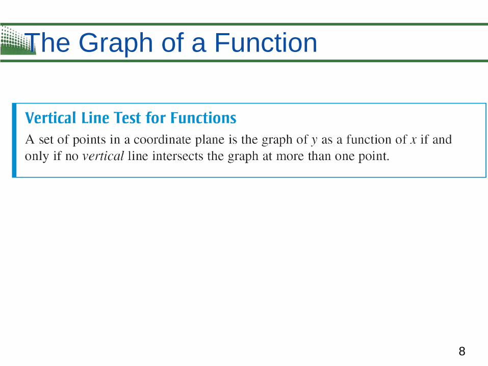
• Use the Vertical Line Test for functions.

• Find the zeros of functions.

• Determine intervals on which functions are

increasing or decreasing and determine relative

maximum and relative minimum values of

functions.

• Determine the average rate of change of a

function.

• Identify even and odd functions.

What You Should Learn

3

The Graph of a Function

4

The Graph of a Function

The graph of a function f : the collection of ordered

pairs (x, f (x)) such that x is in the domain of f.

5

The Graph of a Function

x = the directed distance from the y-axis

y = f (x) = the directed distance from the x-axis

6

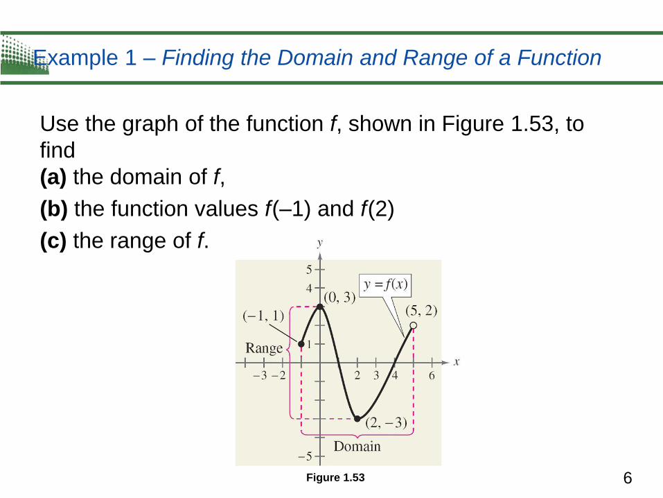
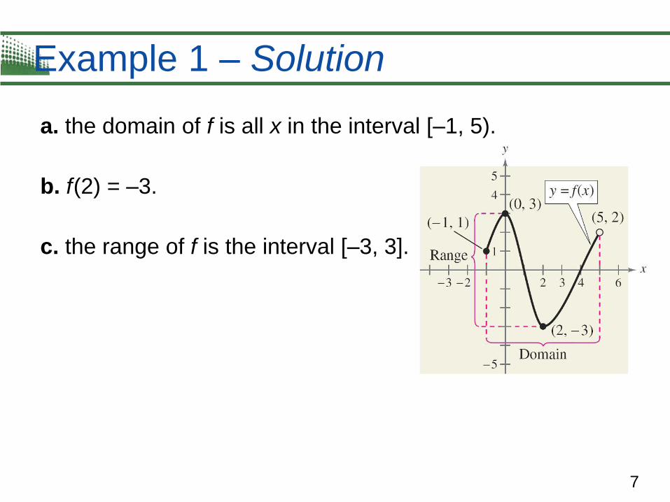
Example 1 – Finding the Domain and Range of a Function

Use the graph of the function f, shown in Figure 1.53, to

find

(a) the domain of f,

(b) the function values f (–1) and f (2)

(c) the range of f.

Figure 1.53

7

Example 1 – Solution

a. the domain of f is all x in the interval [–1, 5).

b. f (2) = –3.

c. the range of f is the interval [–3, 3].

8

The Graph of a Function

9

Zeros of a Function

10

Zeros of a Function

If the graph of a function of x has an x-intercept at (a, 0),

then a is a zero of the function.

11

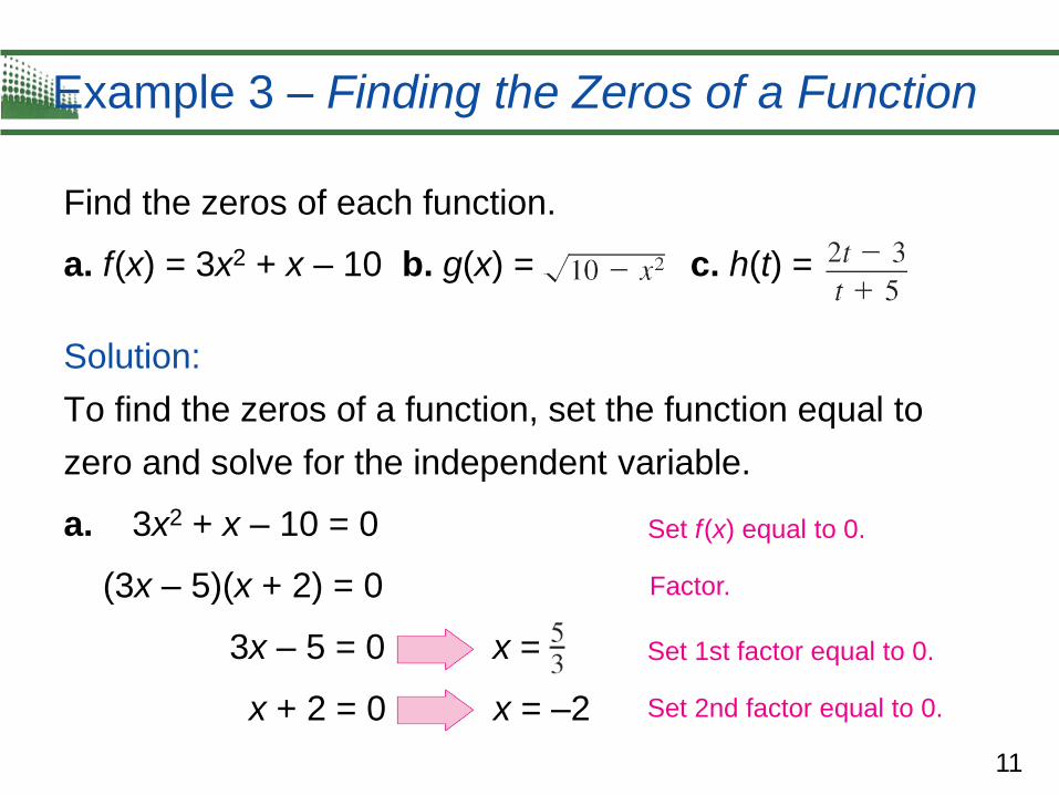
Example 3 – Finding the Zeros of a Function

Find the zeros of each function.

a. f (x) = 3x2 + x – 10 b. g(x) = c. h(t) =

Solution:

To find the zeros of a function, set the function equal to

zero and solve for the independent variable.

a. 3x2 + x – 10 = 0

(3x – 5)(x + 2) = 0

3x – 5 = 0 x =

x + 2 = 0 x = –2

Set f (x) equal to 0.

Factor.

Set 1st factor equal to 0.

Set 2nd factor equal to 0.

12

Example 3 – Solution

The zeros of f are x = and x = –2. In Figure 1.55, note

that the graph of f has ( , 0) and (–2, 0) as its x-intercepts.

Figure 1.55

Zeros of f : x = –2, x =

cont’d

13

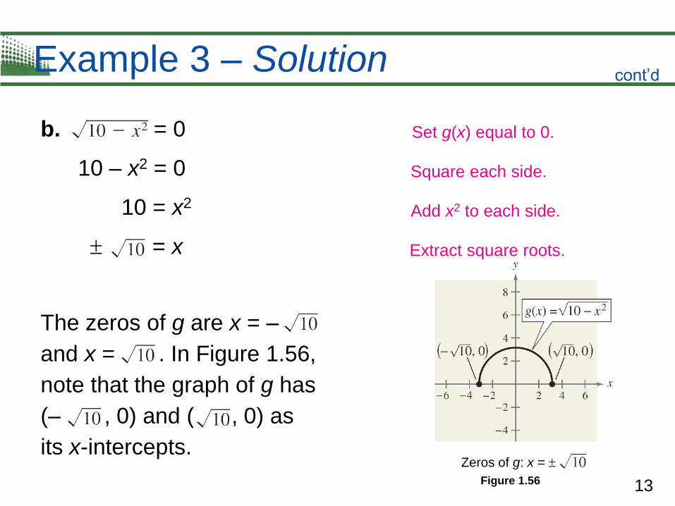
Example 3 – Solution

b. = 0

10 – x2 = 0

10 = x2

= x

The zeros of g are x = –

and x = . In Figure 1.56,

note that the graph of g has

(– , 0) and ( , 0) as

its x-intercepts.

Extract square roots.

Zeros of g: x =

Figure 1.56

Square each side.

Add x2 to each side.

Set g(x) equal to 0.

cont’d

14

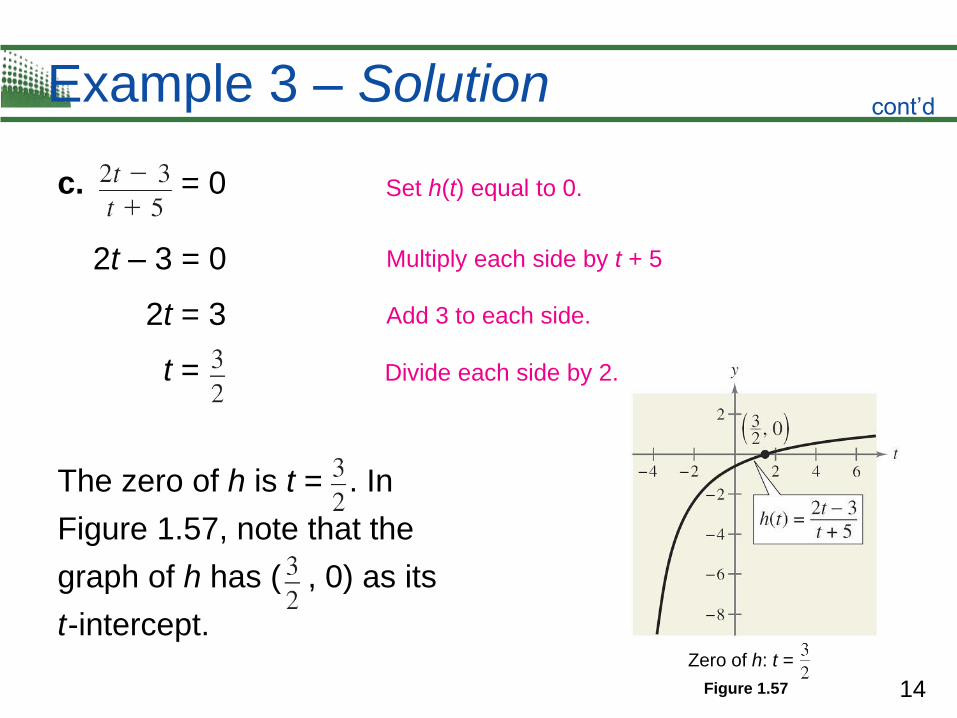
Example 3 – Solution

c. = 0

2t – 3 = 0

2t = 3

t =

The zero of h is t = . In

Figure 1.57, note that the

graph of h has ( , 0) as its

t -intercept.

Divide each side by 2.

Zero of h: t =

Figure 1.57

Set h(t) equal to 0.

Multiply each side by t + 5

Add 3 to each side.

cont’d

15

Increasing and Decreasing Functions

16

Increasing and Decreasing Functions

17

Increasing and Decreasing Functions

18

Example 4 – Increasing and Decreasing Functions

Describe the increasing or decreasing behavior of each

function.

(a) (b) (c)

19

Example 4 – Solution

a. This function is increasing over the entire real line.

20

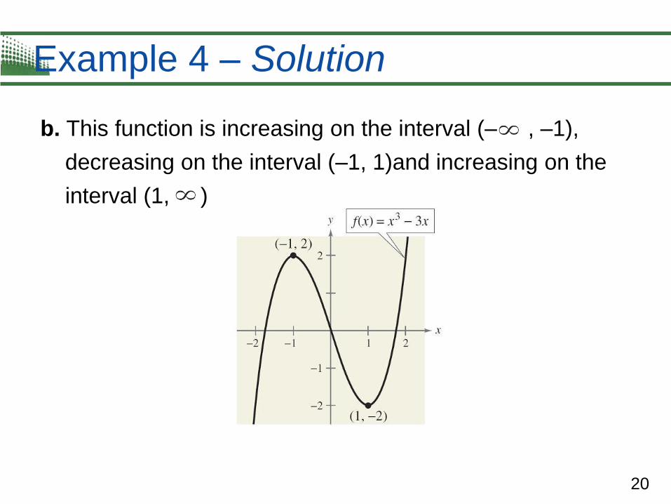
Example 4 – Solution

b. This function is increasing on the interval (– , –1),

decreasing on the interval (–1, 1)and increasing on the

interval (1, )

21

Example 4 – Solution

c. This function is increasing on the interval (– , 0),

constant on the interval (0, 2), and decreasing on the

interval (2, ).

22

Increasing and Decreasing Functions

To help you decide whether a function is increasing,

decreasing, or constant on an interval, you can evaluate

the function for several values of x.

However, calculus is needed to determine, for certain, all

intervals on which a function is increasing, decreasing, or

constant.

23

Increasing and Decreasing Functions

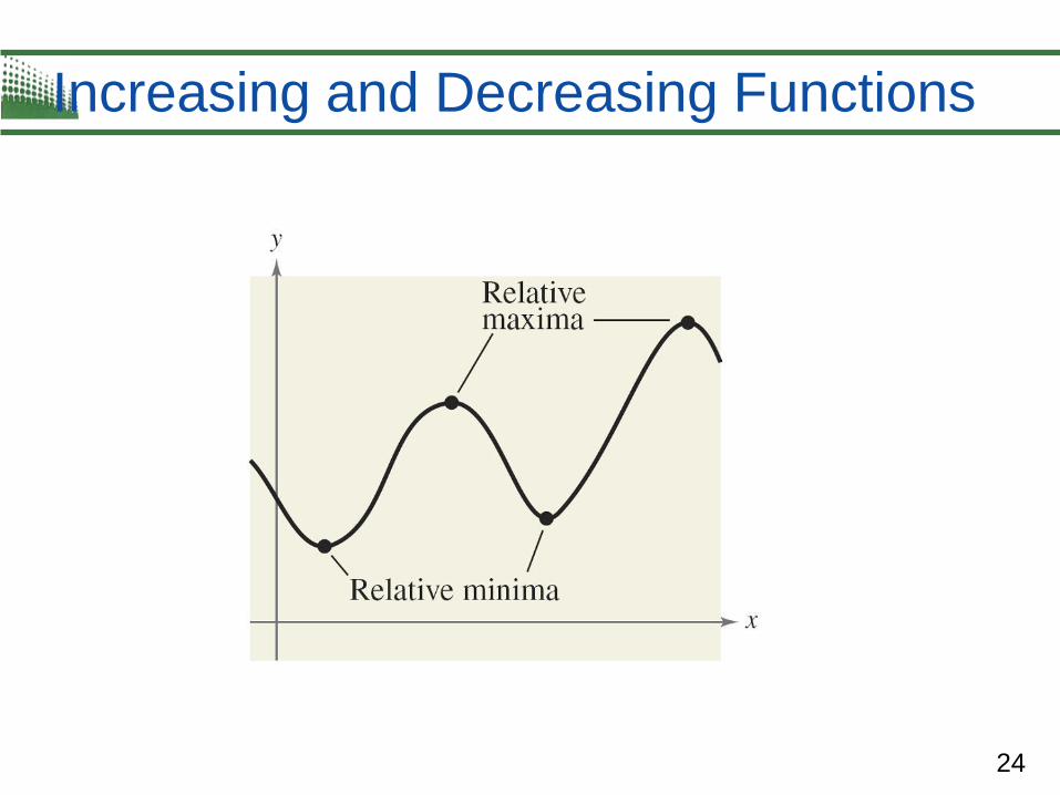
24

Increasing and Decreasing Functions

25

Average Rate of Change

26

Average Rate of Change

the average rate of change between any two points

(x1, f (x1)) and (x2, f (x2)) is the slope of the line through the

two points.

27

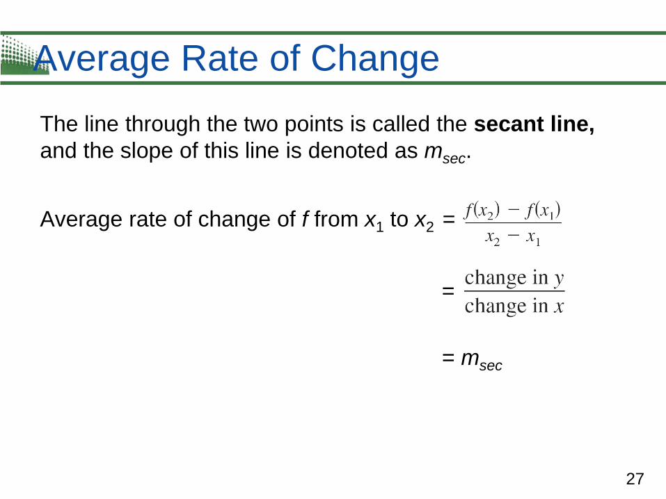
Average Rate of Change

The line through the two points is called the secant line,

and the slope of this line is denoted as msec.

Average rate of change of f from x1 to x2 =

=

= msec

28

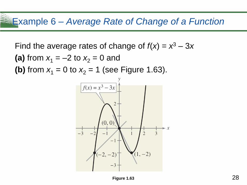
Example 6 – Average Rate of Change of a Function

Find the average rates of change of f (x) = x3 – 3x

(a) from x1 = –2 to x2 = 0 and

(b) from x1 = 0 to x2 = 1 (see Figure 1.63).

Figure 1.63

29

Example 6(a) – Solution

The average rate of change of f from x1 = –2 to x2 = 0 is

Secant line has positive slope.

30

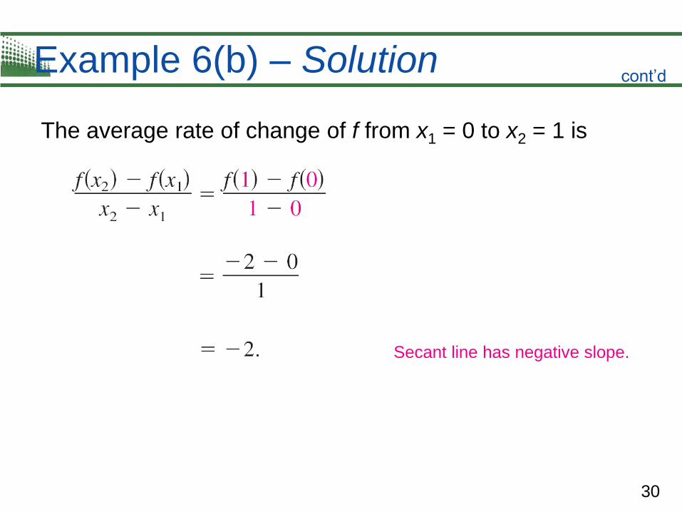
Example 6(b) – Solution

The average rate of change of f from x1 = 0 to x2 = 1 is

Secant line has negative slope.

cont’d

31

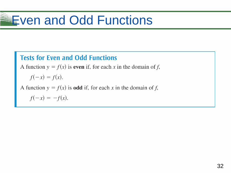
Even and Odd Functions

32

Even and Odd Functions

33

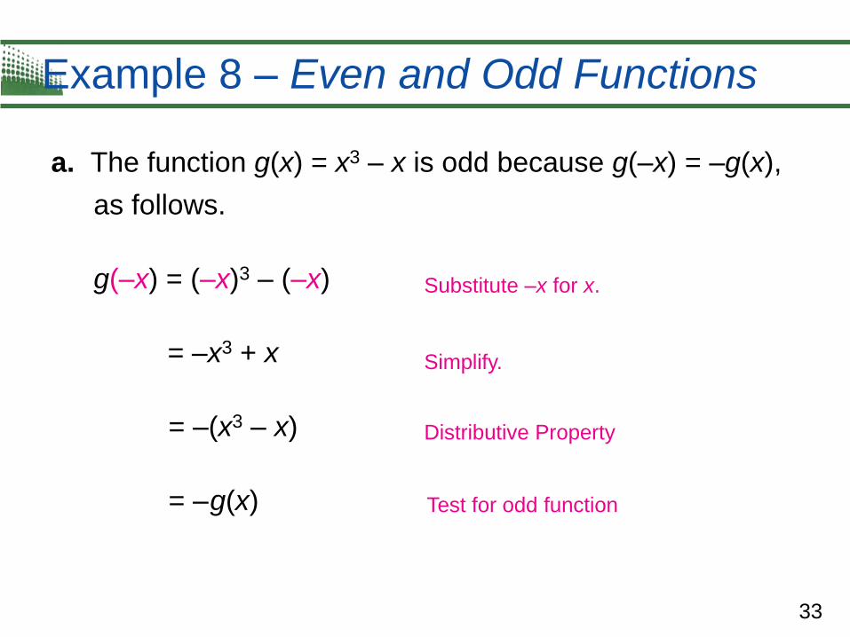
Example 8 – Even and Odd Functions

a. The function g(x) = x3 – x is odd because g(–x) = –g(x),

as follows.

g(–x) = (–x)3 – (–x)

= –x3 + x

= –(x3 – x)

= – g(x)

Substitute –x for x.

Simplify.

Distributive Property

Test for odd function

34

Example 8 – Even and Odd Functions

b. The function h(x) = x2 + 1 is even because h(–x) = h(x),

as follows.

h(–x) = (–x)2 + 1

= x2 + 1

= h(x) Test for even function

Simplify.

Substitute –x for x.

cont’d

35

Example 8 – Even and Odd Functions

The graphs and symmetry of these two functions are

shown in Figure 1.64.

(a) Symmetric to origin: Odd Function (b) Symmetric to y-axis: Even Function

cont’d