ATTACHMENT B

FIRST NOTICE OF PUBLIC AVAILABILITY OF 15-DAY AMENDMENT TEXT

Proposed Amendments to the California Cap on Greenhouse Gas Emissions and Market-Based Compliance Mechanisms Regulation

Post-2020 Industry Assistance Factor Calculations

State of California

AIR RESOURCES BOARD

Release Date: December 21, 2016

Attachment B:

Post-2020 Industry Assistance Factor Calculations In 2011 and 2012, Board Resolutions 11-32 (ARB 2011) and 12-33 (ARB 2012) directed Air Resources Board (ARB) staff to investigate potential improvements to industrial allowance allocation to better meet the Assembly Bill 32 objective to minimize emissions leakage. In response, ARB commissioned three emissions leakage potential studies to inform the development of assistance factors (AF) for Cap-and-Trade Program (Program) allowance allocation to industrial sectors. Based on the results of these leakage studies, ARB staff proposed in Appendix E1 of the 2016 Initial Statement of Reasons to the proposed amendments to the Regulation (ARB 2016A) a methodology by which emissions leakage risk would be assessed and AFs would be developed for the fourth compliance period and beyond. In two informal staff proposals2,3 (ARB 2016B and ARB 2016C) and an October 21, 2016 workshop,4 staff published and presented specific AFs for the majority of industrial sectors covered by the Program. This attachment details additional calculations and updated assumptions based on the Appendix E methodology, informal staff proposals, and stakeholder feedback received since the release of the leakage studies in May 2016. Table 5 provides industry-specific AFs incorporated into the formal first 15-day regulatory amendments. Public Comment on Appendix E and the Informal Staff Proposals To date, staff has received feedback from stakeholders on the appropriateness of using the studies and the appropriateness of assumptions used in translating the studies into sector-specific AFs. Staff has also received feedback on a general difficulty in recreating and verifying staff’s calculations based on the leakage study information and tables available in the informal AF proposals. Basing AFs on sector-specific responses to a marginal Program compliance cost, via measurement of sector-specific historical responses to changes in relative energy prices, aligns compensation with observed sector-specific emissions leakage potential. This led staff to continue revising AFs based in part on the domestic and international leakage studies in this first 15-day regulatory attachment. The food processor study (Hamilton et al. 2016) was not incorporated at this time due to the need for continued analysis of the best means by which to integrate its findings.

1 https://www.arb.ca.gov/regact/2016/capandtrade16/appe.pdf 2 The informal discussion paper for post-2020 AFs for sectors included in the two major leakage studies is

available at https://www.arb.ca.gov/cc/capandtrade/meetings/20161021/ct-af-proposal-102116.pdf and in Attachment E to this 15-day regulatory notice.

3 The informal discussion paper for post-2020 AFs for sectors not included in the two major leakage studies is available at https://www.arb.ca.gov/cc/capandtrade/meetings/20161021/ct-af-proposal-addendum-111016.pdf, and also in Attachment E to this 15-day regulatory notice.

4 Materials from the workshop, and comments received in response to the workshop, are available at https://www.arb.ca.gov/cc/capandtrade/meetings/meetings.htm and in attachment E to this 15-day regulatory notice.

1

Staff was not able to follow the calculations by which the study developed its market transfer measurements. Staff also needs to verify that the elasticities from previous literature used as inputs for the market transfer calculation are appropriate for comparison with the elasticities of the other two studies. Staff will continue to engage with the food processor researchers as part of the amendment process. Based on comments from stakeholders on the difficulty of verifying the October 21, 2016 informal staff proposal’s AF calculations, as well as requests to release the documents used to calculate the informal AFs, staff is publishing a spreadsheet detailing the full calculation of the proposed AFs found in Table 5.5 The spreadsheet entitled “post-2020-af.xlsx” takes as inputs results and information from the domestic (Gray et al. 2016) and international leakage studies (Fowlie et al. 2016), specific (labeled) U.S. Census columns6 and U.S. Census Bureau USA Trade Online trade information.7 The spreadsheet then shows all subsequent calculations used to develop the AFs. The spreadsheet replaces many of the tables found in the informal AF proposals to best address specific methodological questions stakeholders may have for their particular sector (e.g., stakeholders can use the spreadsheet to view all calculations and values used to develop a sector’s international AF component). In response to feedback received during the 45-day comment period and following the October 21, 2016 workshop regarding assumptions used to calculate AFs in the informal staff proposal, staff is revising a key post-2020 AF input—the assumed marginal cost of compliance. The informal staff proposals calculated AFs in part based on an assumed marginal cost of compliance equal to the 2022 auction reserve price. Staff chose 2022, as it would either be the middle or the end of the fourth compliance period (depending on approval of California’s plan for compliance with the federal Clean Power Plan). Staff has revised this assumed marginal cost of compliance to equal the 2025 auction reserve price, increasing the proposed AFs for most sectors. 2025 was chosen as the midpoint of the 2021–2030 period. Staff also received input on potential overestimates of purchased fuels for some sectors in the purchased fuels ratios initially published in Table 2 of the informal staff proposal (ARB 2016B) and Table 5 of the Addendum to October 21, 2016 Informal Staff Proposal (ARB 2016C). Staff has rechecked and updated the ratio for each sector based on data from ARB’s Regulation for the Mandatory Reporting of Greenhouse Gas Emissions (MRR). The updated ratios can be found below in Table 1. In the case of refining, for instance, staff’s estimate of purchased fuels is now lower than in the informal staff proposal. A lower purchased fuels ratio has the effect of increasing allocation relative to the higher purchased fuels ratio found in the two informal staff proposals.

5 The post-2020-af.xlsx spreadsheet is available at https://www.arb.ca.gov/regact/2016/capandtrade16/ post-2020-af.xlsx.

6 Six-digit NAICS U.S. Economic Census data are available at https://factfinder.census.gov/faces/nav/jsf/pages/index.xhtml.

7 Six-digit NAICS U.S. imports and exports data are available with a free account at https://usatrade.census.gov/index.php.

2

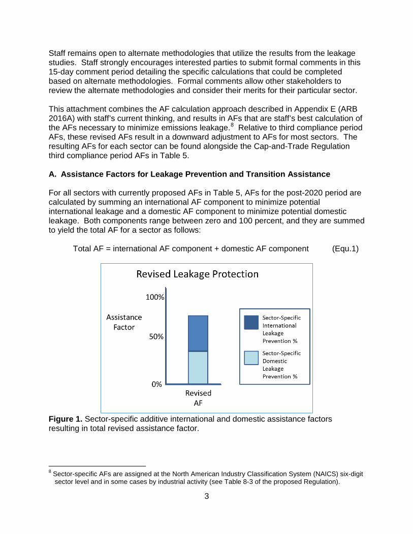
Staff remains open to alternate methodologies that utilize the results from the leakage studies. Staff strongly encourages interested parties to submit formal comments in this 15-day comment period detailing the specific calculations that could be completed based on alternate methodologies. Formal comments allow other stakeholders to review the alternate methodologies and consider their merits for their particular sector. This attachment combines the AF calculation approach described in Appendix E (ARB 2016A) with staff’s current thinking, and results in AFs that are staff’s best calculation of the AFs necessary to minimize emissions leakage.8 Relative to third compliance period AFs, these revised AFs result in a downward adjustment to AFs for most sectors. The resulting AFs for each sector can be found alongside the Cap-and-Trade Regulation third compliance period AFs in Table 5. A. Assistance Factors for Leakage Prevention and Transition Assistance For all sectors with currently proposed AFs in Table 5, AFs for the post-2020 period are calculated by summing an international AF component to minimize potential international leakage and a domestic AF component to minimize potential domestic leakage. Both components range between zero and 100 percent, and they are summed to yield the total AF for a sector as follows:

Total AF = international AF component + domestic AF component (Equ.1)

Figure 1. Sector-specific additive international and domestic assistance factors resulting in total revised assistance factor.

8 Sector-specific AFs are assigned at the North American Industry Classification System (NAICS) six-digit sector level and in some cases by industrial activity (see Table 8-3 of the proposed Regulation).

3

B. Specifics of Post-2020 Emissions Leakage Prevention Methodology for Sectors Analyzed in the International and Domestic Leakage Studies (Studied Sectors) 1. International AF Component Calculation for Studied Sectors

The international AF component is the first component of each sector’s total AF proposed for use for post-2020 allowance allocation.

a. Potential International Emissions Leakage for Certain Manufacturing Sectors without Non-Purchased Fuel9 and Process Emissions

As stated in Appendix E to the 2016 Initial Statement of Reasons, international emissions leakage will be identified and minimized by quantifying international market transfer (IMT), a metric developed by Fowlie et al.10 (international leakage study). IMT is the fraction of every dollar decrease in domestic shipments in response to a marginal GHG price that is offset by an increase in international production (i.e., IMT measures production leakage). Domestic shipments is an approximation of revenue. The international leakage study used the GHG emissions associated with fuels and electricity to calculate the responsiveness, or elasticity, of domestic shipments, domestic exports, and foreign imports for the sector with respect to changes in domestic energy prices similar to the changes experienced upon implementation of a marginal Program compliance cost. For example, the elasticity of domestic exports with respect to domestic energy prices (“exp elasticity” below) is the percentage change in domestic exports with respect to a one percent increase in domestic energy prices. In this attachment, the study-calculated IMTs are referred to as “raw” IMTs. Within this attachment’s companion spreadsheet (post-2020-af.xlsx)11 is the information the international research team provided to ARB staff. The dataset provides annual raw IMT values (“transfer_rate_p50”12) for each year from 2010 through 2015.13 The equation used to calculate the raw IMT for these sectors in a given year “t,” using data from the dataset, is as follows:

Raw IMTi,t = (Ratio_imp_p50i × (Imp_vali,t / Dom_vali,t)) + (Ratio_exp_p50i × (Exp_vali,t / Dom_vali,t)) (Equ. 2)

Where:

9 Non-purchased fuel emissions include emissions from fuels not purchased by the facility (e.g., refinery fuel gas).

10 https://www.arb.ca.gov/cc/capandtrade/meetings/20160518/ucb-intl-leakage.pdf 11 See the tabs titled “description of berkeley dataset,” “berkeley data dictionary,” and “berkeley data” in

the accompanying spreadsheet for international leakage study data. 12 For full transparency, ARB staff has not retitled the columns in each of the three tabs, and has instead

left them as provided by the international leakage research team. 13 Elasticities were calculated for the time period of the study dataset (1993–2012) and were paired with

domestic value, import, and export data from the period 2010 through 2015.

4

“Imp_vali,t” is the value of international imports to the U.S. within sector i for each year 2010 through 2015; “Ratio_imp_p50i” is the import elasticity divided by the domestic shipment elasticity for sector i; “Exp_vali,t” is the value of international exports from the U.S. within sector i for each year 2010 through 2015; “Ratio_exp_p50i” is the export elasticity divided by the domestic shipment elasticity for sector i; and “Dom_vali,t” is the value of domestic shipments for both exports and domestic consumption within sector i for each year 2010 through 2015.

Staff also developed a second estimate of IMT, termed the “regression IMT.” The international research team recommended that staff utilize a regression IMT to harmonize the international AF component across different sectors with similar attributes. Through the regression IMT, similar combinations of trade exposure and energy intensity lead to similar international AF components. Considering other (similar) sectors in developing each sector’s international AF component leverages sector-wide response patterns and relies less on sector-by-sector estimation and calculations. Leveraging sector-wide responses for the international AF component (via the regression IMT) addresses a stakeholder concern that exclusively using sector-specific IMT calculations, or the raw IMT, to develop the international AF component pushes against the limit of available sector-by-sector data. To estimate the regression IMT for each sector, staff ran a pooled linear regression (ordinary least squares, or OLS) between the raw IMT for each manufacturing industry and its trade exposure (TE) and energy intensity. For sectors where raw IMTs were below zero, the raw IMT used in the regression was set equal to zero, and for sectors with raw IMTs exceeding one, the raw IMT used in the regression was set equal to one. Only sectors that are not covered by the Program had raw IMTs below zero or above one; however, these non-covered sectors are relevant to the regression IMT because their values are incorporated into the regression. This process provided linear coefficients (i.e., B0, B1, and B2) via equation 3: Raw IMTi,t = B0 + B1 × TEi,t + B2 × (energy intensityi,t) + errori,t (Equ. 3) Where:

“Raw IMTi,t” is sector i's IMT for year t from the dataset; “TEi,t” is sector i's trade exposure for year t from the dataset;

5

“energy intensityi,t” is sector i's energy intensity for year t from the dataset; “Bk” is the industry-wide relationship between variable k and raw IMT; and “errori,t” is the difference between “Raw IMTi,t” and the right-hand side of the equation excluding “errori,t” at the OLS-regression-estimated “Bk”.

The linear coefficients estimated in equation 3 were then used to calculate the regression IMT value for a sector based on its TE and energy intensity. Each industry’s regression IMT was calculated using equation 4, where estBk is the estimated value of Bk from the pooled OLS regression above:14

Regression IMTi,t = estB0 + estB1 × (TEi,t) + estB2 × (energy intensityi,t) (Equ. 4) Staff used single multi-year IMT values based on the average of 2010 through 2015 annual raw and regression IMTs. This averaging was weighted by domestic shipments (i.e., IMTs from years with more sector-specific domestic economic activity were given more weight in staff’s calculation of the multi-year IMT). Table 2 shows the raw IMT, regression IMT, and the IMT value used to calculate the total AF in equation 1 for each studied sector.15 When calculating the total AF for a sector, staff set the international assistance factor component equal to the average of the raw IMT and regression IMT. Regression IMT values were applied in this manner because, as described in the international leakage study, some of the raw IMT values were noisy and not in line with expectations (e.g., high trade exposure but low raw IMT). Figure 2 shows a raw IMT and regression IMT for a hypothetical sector. The raw IMT is 0.07 and the regression IMT—calculated from the sector’s energy intensity, trade exposure, and equation 4—is 0.15. When calculating the total AF by equation 1 for this hypothetical sector, the international AF component would be assigned at the average of these two values: 0.11.

14 These coefficients are highlighted in orange in the “berkeley_spreadsheet” tab of the accompanying spreadsheet, and can be reproduced using the “Regression” option of the Data Analysis add-in included in Microsoft® Excel® with the variables used in Equation 3 in columns AG, AH, and AI. 15 Within the accompanying spreadsheet, these values can be found for studied sectors in columns G, H and I of the “results” tab. See section D for a discussion of the international AF component calculation for non-studied sectors.

6

Figure 2. Raw IMT and regression IMT for a hypothetical sector.

b. Potential International Emissions Leakage for Studied Sectors with Non-Purchased Fuel and/or Process Emissions

For sectors that have non-purchased fuel emissions and/or process emissions in addition to energy-related emissions, staff used an upward adjustment to the energy intensity used to estimate the sector’s regression IMT (i.e., the energy intensity in equation 4 was increased). Non-purchased fuel emissions include emissions from fuels not reported to the U.S. Census Bureau as part of the Annual Survey of Manufacturing (ASM) data used by the international leakage study to establish sector-specific energy expenditures.16 For example, refinery fuel gas is a byproduct of onsite processes at refineries. Refineries do not purchase this fuel, so it is not included in the ASM data, but emissions from combusting refinery fuel gas incur a compliance obligation in the Program. Process emissions are non-combustion emissions, such as the process emissions arising from cement production. For sectors with non-purchased fuel and process emissions, the third column of Table 1 provides the ratio of emissions captured by the international leakage study to emissions covered with a compliance obligation in the Program (covered emissions) based on data collected under MRR. For these sectors, the revised energy intensity used to develop each sector’s regression IMT (i.e., the energy intensity used in equation 4) was calculated as:

Revised equation 4 energy intensity = study energy intensity / F (Equ. 5)

16 ASM, and thus IMT, includes coal and coke expenditures, so an adjustment has not been applied to IMT for coal and coke consumption.

7

Where: “study energy intensity” is the energy intensity calculated by the international leakage study based on ASM purchased fuel data; and “F” is the fraction of covered emissions from the consumption of purchased fuels and process emissions based on MRR data (i.e., 1 – non-purchased fuel emissions and process emissions). These are the values presented in the third column of Table 1.

The cement sector’s non-purchased fuel emissions were not adjusted by coal and coke consumption; these fuels were included in the fuels report used as the input to the international study in determining energy intensity. This difference in fuels covered results in a significantly larger purchased fuels fraction used in the regression IMT determination, and a lower purchased fuels fraction used for domestic leakage calculations calculated through the methodology of section B.2.a and B.2.d for the cement sector. The formula used to calculate purchased fuel and process emissions for use in the international AF component calculation was:

F = (purchased electricity emissions + purchased natural gas emissions + purchased steam emissions + purchased coal emissions + purchased coke emissions) / (covered emissions + purchased electricity emissions + purchased steam emissions – sold electricity emissions – sold steam emissions) (Equ. 6)

The data source for inputs to equation 6 were 2012–2015 MRR data for all covered entities in each sector except cement. For the cement sector, calculations used MRR data from 2013–2015 for all covered entities. In the accompanying spreadsheet, these ratios can be found in the “purchased emissions” tab in the “International AF Component Ratio” column. While industrial facilities do not have a direct compliance obligation on the emissions associated with electricity purchases, they do receive a pass through of the cost of compliance associated with these emissions via their electricity rates. Therefore, electricity emissions show up in the numerator, as a source of compliance cost accounted for by the studies. Facilities with the ability to sell electricity and steam are expected to pass through the cost of compliance into the contracts under which they sell the electricity and steam.

2. Potential Domestic Emissions Leakage for Studied Sectors

a. Potential Domestic Leakage for Studied Sectors without Non-Purchased Fuels and/or without Process Emissions: Developing Domestic Drops

8

The domestic leakage study17 used plant-level U.S. Census data to simulate the effects of a marginal Program price-driven increase in operating costs on manufacturing sectors in California through increased electricity and natural gas prices. The study measured the decrease in output, value added, and employment for each sector. The increase in California operating cost is driven by increased electricity and natural gas prices, which escalate with allowance prices. The domestic leakage study simulated industry responses for a marginal compliance cost of $24.88 per MTCO2e in 2016 dollars with varying domestic AF components. This represents the 2030 auction reserve price in 2016 dollars. In developing domestic AF components, staff is applying the lower 2025 auction reserve price of $19.70, in real 2015 dollars, used by the Standardized Regulatory Impact Assessment (SRIA).18 Staff used the output and value added responses to an allowance value to assess potential domestic emissions leakage caused by the Program. Staff also developed and applied two additional domestic leakage estimates. Similar to the regression IMT, these are based on industry-wide regressions of the drop in value added or drop in output on each industry’s energy intensity, termed “regressed domestic value added drop” and “regressed output drop,” respectively. Each of these four methods is referred to as a domestic drop (DD) methodology. Staff is basing each sector’s DD for application in developing the revised AFs on the average of domestic value added drop, domestic output drop, regressed domestic value added drop, and regressed domestic output drop. Domestic value added drop—the first DD methodology—can be found in Table A1 of the domestic leakage study, which is reproduced in the accompanying spreadsheet “valadd_dd” tab. These are domestic value added drop values for a range of domestic AF component values from zero, indicating no allowance allocation, up to 90 percent allowance allocation, in 10 percent increments.19 Domestic value added drop for a given sector generally decreases to smaller negative values as the AF increases from left to right in the ”valadd_tab,” indicating that domestic value added decreases less in response to a marginal compliance cost as AF values increase. For the industrial sectors studied, Figure 3 plots the domestic value added drops from the column B of the “valadd_dd” tab (i.e., those with an AF equal to zero, indicating no allowance allocation at the 2030 auction reserve price) relative to natural gas and electricity expenditures and a $24.88 (2016 dollars) per MTCO2e marginal compliance cost.

17 https://www.arb.ca.gov/cc/capandtrade/meetings/20160518/rff-domestic-leakage.pdf 18 https://www.arb.ca.gov/regact/2016/capandtrade16/appc.pdf, and included in the “compliance cost” tab

of the accompanying spreadsheet. 19 Assessment at increments of 10 percent results in higher AFs than those that would prevent a 7

percent drop (at the 2025 auction reserve price) in the relevant metric. In other words, if a 7 percent domestic (study) output drop is experienced at a 36 percent AF, the domestic AF component as measured by the study’s output metric would be 40 percent, not 30 percent.

9

Figure 3. Percent reduction in California value added for various industrial sectors with AF equal to zero and a $24.88 (2016 dollars) per MTCO2e marginal compliance cost from the domestic leakage study. As discussed in Appendix E, the authors of the domestic leakage study (Resources for the Future) also supplied information on domestic output drop in response to a $24.88 marginal compliance cost; these values are available in the “output_dd” tab of the accompanying spreadsheet. Similar to the domestic value added drop values, the domestic output drop tables present domestic output drops for a range of domestic AF component values from zero up to 90 percent, and increasing allowance allocation generally decreases the domestic output drop. Figure 4 plots the domestic output drops from column B of the “output_dd” tab (i.e., those with an AF equal to zero, indicating no allowance allocation at the 2030 auction reserve price) relative to natural gas and electricity expenditures and a $24.88 per MTCO2e marginal compliance cost.

10

Figure 4. Percent reduction in California output for various industrial sectors with AF equal to zero and a $24.88/MTCO2e marginal compliance cost from the domestic leakage study. As can be seen in Figures 3 and 4, the domestic leakage study calculated counterintuitive positive domestic value added and domestic output responses to increased energy prices for some California sectors. Staff has developed a methodology to provide allocation for sectors with these counterintuitive responses. Broadly, when covered sectors had limited or positive changes (cheese manufacturing, wineries, biological product (except diagnostic) manufacturing, and rolled steel shape manufacturing) in value added and/or output in response to the compliance cost relative to their energy intensity, staff adjusted the response downward to match an average level of decrease in value added and/or output based on sectors with similar energy intensities. While these individual sectors showed positive responses, the trend of the overall studied sectors conforms with expectations—that is, value added and output decrease in response to increased energy prices, and the impacts are more negative for sectors with higher energy intensities. For sectors with high energy intensities, value added drops (Figure 3) and output drops (Figure 4) from the domestic leakage study were very negative.

11

Figures 3 and 4 generally show a curved negative relationship between value added and energy intensity, and output drop and energy intensity. Informed by this relationship, staff developed a regression to correlate domestic value added drop to energy intensity (Equation 8 with resulting values in column H of the “regressed_valadd_dd” tab of the accompanying spreadsheet). Staff also developed a correlation of domestic output drop to energy intensity (Equation 10 with resulting values in column G of the “regressed_output_dd” tab of the accompanying spreadsheet). In the sectors for which value added drop and/or output drop were positive, the drops were lowered to zero (“ARB value added” and “ARB output” in the respective tabs) prior to running the regression. 20 Similar to the regression IMT, using regressions for DD allowed for increased compensation to sectors with unexpectedly low output and value added responses relative to their energy intensities (i.e., Figures 3 and 4 show a more negative response at greater energy intensities for most sectors). This has the effect of increasing allocation for these sectors. The domestic value added drop regression is a pooled linear regression (OLS) with all studied sectors’ domestic value added drop at a zero assistance factor (column D of the “valadd_dd” tab of the accompanying spreadsheet) regressed on the natural log of the sector’s energy intensity. The regression equation is as follows:

DVAi,study,0 = B0 + B1 × ln(energy intensityi) + errori (Equ. 7) Where:

“DVAi,study,0” is the domestic value added drop for sector “i” with zero assistance factor from the domestic leakage study, which can be found in column D of the “valadd_dd” tab; and “errori” is the difference between DVAi,study,0 and the right-hand side of the equation (i.e., equation 7), excluding errori.

The regressed domestic value added drop with a zero assistance factor for a sector is then calculated by the following equation:

DVAi,regressed,0 = estB0 + estB1 × ln(energy intensityi) (Equ. 8) Where:

“DVAi,regressed,0” is the regression domestic value added drop for sector “i” with zero assistance factor, which are presented as column H of the “regressed_valadd_dd” tab of the accompanying spreadsheet, and

20 When the left-hand-side of equations 7 and 10 are more negative, estBk in equations 8 and 11 are more negative, resulting in greater (more negative) regressed value added and regressed output drops.

12

“estBk” is the OLS estimate of the coefficient Bk resulting from the pooled OLS regression of equation 6.21

With the regression domestic value added drop at zero assistance factor established for each sector, staff then populated the remainder of the “regressed_valadd_dd” tab for increasing values of AF based on the following formula:

DVAi,regressed,X = DVAi,regressed,0 × (1 – X) (Equ. 9) Where:

“DVAi,regressed,X” is the regression domestic value added drop for sector “i” with an assistance factor equal to X, where X is one of the various AF values reported in the “regressed_valadd_dd” tab of the accompanying spreadsheet.

Regressed output drop is calculated using the same general method as regressed value added drop:

Output Dropi,study,0 = B0 + B1 × ln(energy intensityi) + errori (Equ. 10) Where:

“Output Dropi,study,0” is the domestic output drop for sector “i” with zero assistance factor from the domestic leakage study, which can be found in column D of the “output_dd” tab of the accompanying spreadsheet; and “errori” is the difference between DVAi,study,0 and the right-hand side of the equation (i.e., equation 10), excluding errori.

Each sector’s regressed domestic output drop with a zero assistance factor is then calculated by the following equation:

Output Dropi,regressed,0 = estB0 + estB1 × ln(energy intensityi) (Equ. 11) Where:

“Output Dropi,regressed,0” is the regression domestic output drop for sector “i” with zero assistance factor, which are presented as column G of the “regressed_output_dd” tab of the accompanying spreadsheet, and “estBk” is the OLS estimate of the coefficient Bk resulting from equation 10.22

21 These estBk coefficients are the coefficients estimated in equation 10, where k is either 0 or 1. The estimates are available in the trendline formula for the “log energy intensity vs value added drop 0AF” graph and columns F and G of the “regressed_valadd_dd” tab of the accompanying spreadsheet.

22 These coefficients are available in the trendline formula for the “log energy intensity vs output drop 0AF” graph and columns E and F of the “regressed_valadd_dd” tab of the accompanying spreadsheet.

13

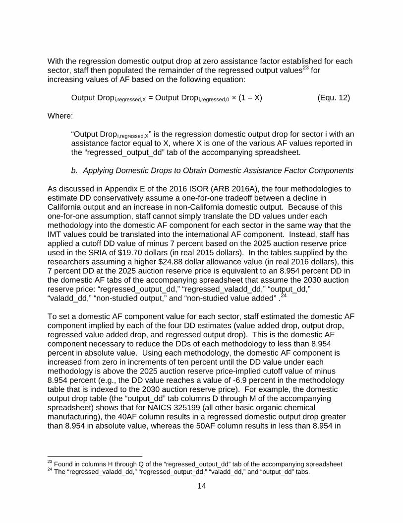
With the regression domestic output drop at zero assistance factor established for each sector, staff then populated the remainder of the regressed output values23 for increasing values of AF based on the following equation:

Output Dropi,regressed,X = Output Dropi,regressed,0 × (1 – X) (Equ. 12) Where:

“Output Dropi,regressed,X” is the regression domestic output drop for sector i with an assistance factor equal to X, where X is one of the various AF values reported in the “regressed_output_dd” tab of the accompanying spreadsheet.

b. Applying Domestic Drops to Obtain Domestic Assistance Factor Components

As discussed in Appendix E of the 2016 ISOR (ARB 2016A), the four methodologies to estimate DD conservatively assume a one-for-one tradeoff between a decline in California output and an increase in non-California domestic output. Because of this one-for-one assumption, staff cannot simply translate the DD values under each methodology into the domestic AF component for each sector in the same way that the IMT values could be translated into the international AF component. Instead, staff has applied a cutoff DD value of minus 7 percent based on the 2025 auction reserve price used in the SRIA of $19.70 dollars (in real 2015 dollars). In the tables supplied by the researchers assuming a higher $24.88 dollar allowance value (in real 2016 dollars), this 7 percent DD at the 2025 auction reserve price is equivalent to an 8.954 percent DD in the domestic AF tabs of the accompanying spreadsheet that assume the 2030 auction reserve price: “regressed_output_dd,” “regressed_valadd_dd,” “output_dd,” “valadd_dd,” “non-studied output,” and “non-studied value added” .24 To set a domestic AF component value for each sector, staff estimated the domestic AF component implied by each of the four DD estimates (value added drop, output drop, regressed value added drop, and regressed output drop). This is the domestic AF component necessary to reduce the DDs of each methodology to less than 8.954 percent in absolute value. Using each methodology, the domestic AF component is increased from zero in increments of ten percent until the DD value under each methodology is above the 2025 auction reserve price-implied cutoff value of minus 8.954 percent (e.g., the DD value reaches a value of -6.9 percent in the methodology table that is indexed to the 2030 auction reserve price). For example, the domestic output drop table (the “output_dd” tab columns D through M of the accompanying spreadsheet) shows that for NAICS 325199 (all other basic organic chemical manufacturing), the 40AF column results in a regressed domestic output drop greater than 8.954 in absolute value, whereas the 50AF column results in less than 8.954 in

23 Found in columns H through Q of the “regressed_output_dd” tab of the accompanying spreadsheet 24 The “regressed_valadd_dd,” “regressed_output_dd,” “valadd_dd,” and “output_dd” tabs.

14

absolute value (-8.6). Thus, the domestic AF component implied by the regressed domestic output drop methodology for NAICS 325199 is 50 percent.25

c. Selection of 7 Percent Domestic Drop Cutoff Staff selected 7 percent as the cutoff DD based on an analysis of historical variation in the manufacturing sector from 1958 through 2011. Staff used inflation-adjusted (real) output and value added data for the manufacturing sectors taken from the National Bureau of Economic Research (NBER) Center for Economic Studies Manufacturing Industry Database (NBER, 2016). Seven percent represents staff’s calculation of typical one-year inflation-adjusted decreases in output and value added based on overall industrial trends for all manufacturing sectors. Staff used one-year real percentage changes in output and value added to match the domestic study’s one-year short-run analysis used as an input to the domestic AF component. Staff calculated a 7 percent domestic drop by taking the average of value added and output measures of (1) year-over-year percentage drops in economic activity in years where economic activity declined, (2) year-over-year percentage drops in economic activity excluding changes from 200726 onward (to calculate drops while omitting the significant reductions in growth of the Great Recession), and (3) average sector-specific percentage growth minus one half the sector-specific standard deviation in percentage growth. The average of these measures was 7.2 percent. Staff rounded to 7 percent for use as the cutoff DD (increasing the domestic AF component for some sectors). The 7 percent is representative of historical domestic drops that occur in the absence of the Program. The domestic leakage study performed both a long-run (5-year) and short-run (1-year) analysis showing leakage risk over each time period. In the long-run analysis, almost every sector adapts to the Program and doesn’t face a risk of leakage. Since the five-year changes in the domestic study’s Table 6 in response to a compliance cost were much smaller than the one-year changes used for the domestic AF component for most sectors, use of the one-year domestic study results in AFs that are likely higher than what is needed to prevent against emissions leakage over periods longer than one year. However, some sectors that showed odd responses to the Program (i.e., they gained business as a result) over a 5-year horizon. Based on this counterintuitive response, staff avoided the sector-specific long-run values in calculating the assistance factors. Domestic and international responses to changes in energy prices as calculated by the leakage studies are also predicated on 100 percent cost pass through of GHG costs, based on higher emissions intensive electricity than is available in California as a result of the RPS program. The international AF component and domestic AF component are added together to arrive at the AFs proposed for the post-2020 period under equation 1. To the extent that a sector has a positive international AF component, this additional compensation exceeds what is necessary to

25 Domestic AF components for studied sectors under each methodology can be found in columns J through M of the “results” tab in the accompanying spreadsheet.

26 i.e., excluding the percentage change from 2007 to 2008, 2008 to 2009, 2009 to 2010, and 2010 to 2011

15

prevent a 7 percent drop in the domestic metric. This additional compensation via the international AF component works to reduce the domestic drop further.

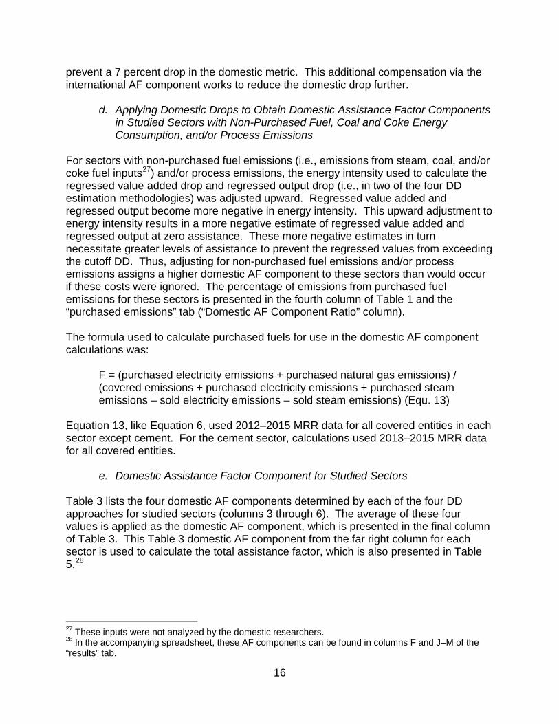
d. Applying Domestic Drops to Obtain Domestic Assistance Factor Components in Studied Sectors with Non-Purchased Fuel, Coal and Coke Energy Consumption, and/or Process Emissions

For sectors with non-purchased fuel emissions (i.e., emissions from steam, coal, and/or coke fuel inputs27) and/or process emissions, the energy intensity used to calculate the regressed value added drop and regressed output drop (i.e., in two of the four DD estimation methodologies) was adjusted upward. Regressed value added and regressed output become more negative in energy intensity. This upward adjustment to energy intensity results in a more negative estimate of regressed value added and regressed output at zero assistance. These more negative estimates in turn necessitate greater levels of assistance to prevent the regressed values from exceeding the cutoff DD. Thus, adjusting for non-purchased fuel emissions and/or process emissions assigns a higher domestic AF component to these sectors than would occur if these costs were ignored. The percentage of emissions from purchased fuel emissions for these sectors is presented in the fourth column of Table 1 and the “purchased emissions” tab (“Domestic AF Component Ratio” column). The formula used to calculate purchased fuels for use in the domestic AF component calculations was:

F = (purchased electricity emissions + purchased natural gas emissions) / (covered emissions + purchased electricity emissions + purchased steam emissions – sold electricity emissions – sold steam emissions) (Equ. 13)

Equation 13, like Equation 6, used 2012–2015 MRR data for all covered entities in each sector except cement. For the cement sector, calculations used 2013–2015 MRR data for all covered entities.

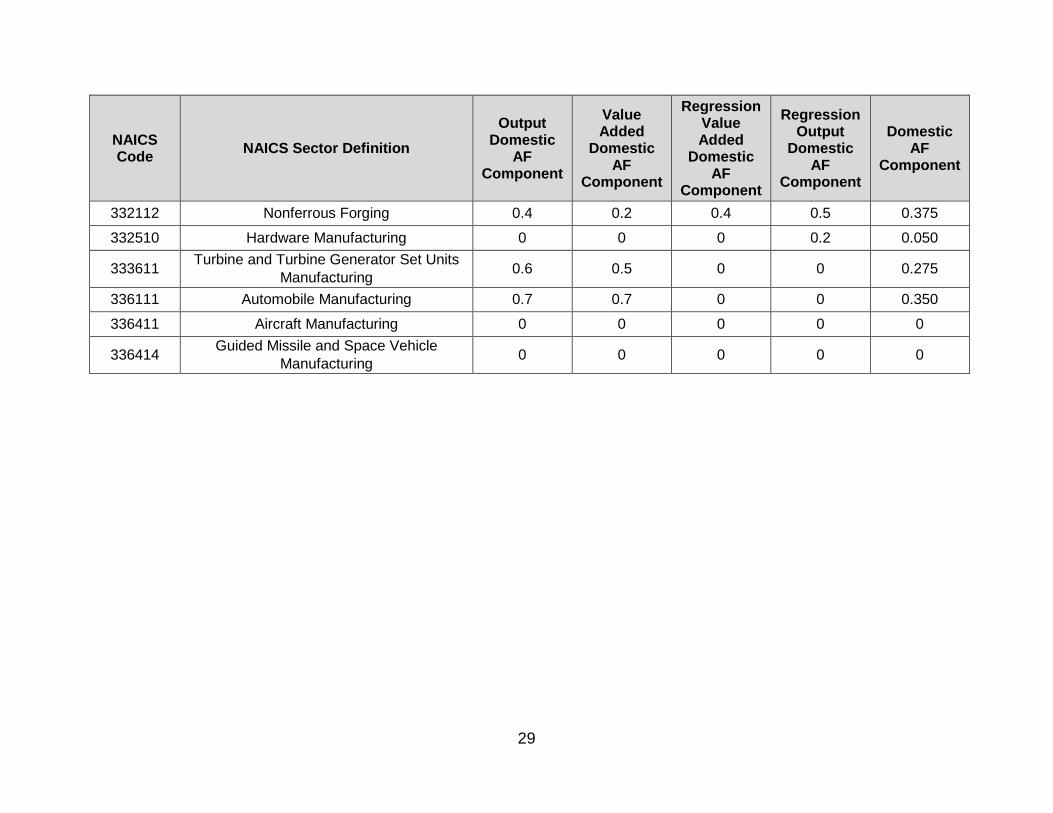
e. Domestic Assistance Factor Component for Studied Sectors Table 3 lists the four domestic AF components determined by each of the four DD approaches for studied sectors (columns 3 through 6). The average of these four values is applied as the domestic AF component, which is presented in the final column of Table 3. This Table 3 domestic AF component from the far right column for each sector is used to calculate the total assistance factor, which is also presented in Table 5.28

27 These inputs were not analyzed by the domestic researchers. 28 In the accompanying spreadsheet, these AF components can be found in columns F and J–M of the “results” tab.

16

C. Food Processing Sectors Along with the domestic and international studies, a third study (food processor study)29 focused specifically on select food processing industries was conducted by a team of researchers led by California Polytechnic Institute, San Luis Obispo. This study focused on leakage risk in the tomato processing (NAICS 311421), wet corn milling (NAICS 311221), sugar (31131), and cheese (311513) manufacturing sectors. Staff appreciated the difficulty of obtaining results given limited aggregated data on these food processing industries. The required assumptions these limited data necessitated, however, made it more appealing for staff to use the systematic methodologies of the domestic and international studies, which are uniform across all of the studied sectors. The international study provided estimates of IMT for all four of the food processor study sectors, making it possible to apply the IMT methodology described in section B. The domestic study provided domestic drop for all but wet corn milling (NAICS 311221). For wet corn milling, staff employed the domestic drop methodology used for non-studied sectors described in section D. Staff is working with the researchers to better understand the food processor study. Staff will continue to evaluate the potential to incorporate the study into development of AFs for these four sectors.. D. Emissions Leakage for Sectors Not Evaluated by the Studies

1. Overview The leakage studies used to develop the proposed post-2020 AFs for the manufacturing sectors analyzed potential industrial emissions leakage risk for most manufacturing sectors covered by the Program (i.e., most sectors assigned a NAICS code starting with 3). Non-manufacturing sectors with NAICS codes starting with 1, 2, and 4 and other sectors were not analyzed by these studies. Sectors not analyzed by the domestic and international studies are shown in Table 4, and are referred to in this attachment as “non-studied sectors.” Table 6 lists the subset of Table 4 sectors that are manufacturing sectors, and identifies which sectors have been analyzed by at least one of the leakage studies. Because some combination of raw IMT, value added DD, and output DD values for these non-studied sectors are unavailable, international AF components and domestic AF components for these sectors were estimated by matching each non-studied sector based on its energy intensity and trade exposure using the processes described below. The estimated AF components were then used as inputs to equation 1 in calculating the total AF proposed for the post-2020 AFs that are found in Table 5. For manufacturing sectors with one leakage analysis available (as identified in Table 6), it was possible to use that study’s results (e.g., wet corn milling sector was analyzed by the international leakage researchers, and can use the international AF component methodology from Section B above). In these cases, the AFs in Table 5 use the studied

29 https://www.arb.ca.gov/cc/capandtrade/meetings/20160518/calpoly-food-process-leakage.pdf

17

sector methodology for the component where possible. For the other AF component, the methodology below was used.

2. International AF Component for Sectors Not Analyzed in the International and Domestic Leakage Studies (Non-Studied Sectors)

For the international AF component (IMT) of a non-studied sector, publicly available six-digit NAICS value added data from 2007 and 2012 U.S. Census and USA Trade Online import and export data30 are combined to calculate an average energy intensity and trade exposure. The energy intensity and trade exposure are then used to calculate an IMT value using equation 4. The “non-studied sectors” tab of the accompanying spreadsheet lists the energy intensities, trade exposure values, and IMTs for the non-studied sectors that were determined using this method. The calculated IMT values are set equal to the international AF component for these sectors. The detailed calculations of the trade exposures and energy intensities (adjusted for emissions associated with non-studied fuels and process emissions) can be found in the “census_data” tab of the accompanying spreadsheet.31 These IMT values can also be found in column 6 of Table 4. For the soda ash, diatomite, and rare earth production sector (NAICS 212299, 212391, and 212399), the U.S. Geological Survey (USGS) reports subsector-specific trade exposure calculations (USGS 2016A, USGS 2016B).32 Where available, these trade exposures replaced trade exposures calculated using U.S. Census information. As part of the amendment process, staff is reviewing whether or not it is possible to conduct a similar sub-sector trade exposure analysis for borate production (also NAICS 212391).

3. Domestic AF Component for Non-Studied Sectors The domestic study analyzed the responsiveness in output and value added to changes in electricity and natural gas prices. This responsiveness was used to measure the effect of a marginal GHG cost on domestic leakage. Responsiveness is driven in part by the fraction of total costs coming from energy consumption; this fraction is called “energy intensity.” The greater the sector-specific energy intensity, the greater the sector-specific cost impact of a marginal GHG cost. Two DD measures used for determining the domestic AF component for studied sectors use a regression approach of the study’s domestic drop measurements on energy

30 USA Trade Online: total NAICS six-digit level exports and CIF imports values. CIF (cost, insurance, freight) imports is the “landed value of the merchandise at the first port of arrival in the United States. It is computed by adding import charges to the Customs value and therefore excludes U.S. import duties.” (USA Trade Online glossary of terms, available through log-in at https://usatrade.census.gov/). These data are reproduced in columns D through G of the “census_data” tab in the accompanying spreadsheet

31 U.S. Census data inputs to this tab can be found in the tabs titled “naics_2_2007_economic_census,” “naics_2_2012_economic_census,” “naics_3_2007_economic_census,” “naics_3_2012_economic_census,” and “sector_4881_census.”

32 In the accompanying spreadsheet, these calculations are available in the “USGS data” tab

18

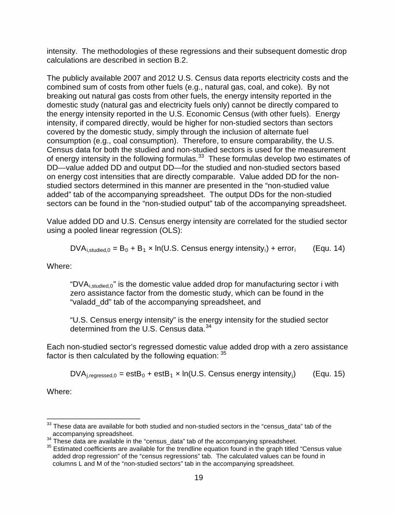
intensity. The methodologies of these regressions and their subsequent domestic drop calculations are described in section B.2. The publicly available 2007 and 2012 U.S. Census data reports electricity costs and the combined sum of costs from other fuels (e.g., natural gas, coal, and coke). By not breaking out natural gas costs from other fuels, the energy intensity reported in the domestic study (natural gas and electricity fuels only) cannot be directly compared to the energy intensity reported in the U.S. Economic Census (with other fuels). Energy intensity, if compared directly, would be higher for non-studied sectors than sectors covered by the domestic study, simply through the inclusion of alternate fuel consumption (e.g., coal consumption). Therefore, to ensure comparability, the U.S. Census data for both the studied and non-studied sectors is used for the measurement of energy intensity in the following formulas.33 These formulas develop two estimates of DD—value added DD and output DD—for the studied and non-studied sectors based on energy cost intensities that are directly comparable. Value added DD for the non-studied sectors determined in this manner are presented in the “non-studied value added” tab of the accompanying spreadsheet. The output DDs for the non-studied sectors can be found in the “non-studied output” tab of the accompanying spreadsheet. Value added DD and U.S. Census energy intensity are correlated for the studied sector using a pooled linear regression (OLS):

DVAi,studied,0 = B0 + B1 × ln(U.S. Census energy intensityi) + errori (Equ. 14) Where:

“DVAi,studied,0” is the domestic value added drop for manufacturing sector i with zero assistance factor from the domestic study, which can be found in the “valadd_dd” tab of the accompanying spreadsheet, and

“U.S. Census energy intensity” is the energy intensity for the studied sector determined from the U.S. Census data.34

Each non-studied sector’s regressed domestic value added drop with a zero assistance factor is then calculated by the following equation: 35

DVAj,regressed,0 = estB0 + estB1 × ln(U.S. Census energy intensityj) (Equ. 15) Where:

33 These data are available for both studied and non-studied sectors in the “census_data” tab of the accompanying spreadsheet.

34 These data are available in the “census_data” tab of the accompanying spreadsheet. 35 Estimated coefficients are available for the trendline equation found in the graph titled “Census value

added drop regression” of the “census regressions” tab. The calculated values can be found in columns L and M of the “non-studied sectors” tab in the accompanying spreadsheet.

19

“DVAj,regressed,0” is the regression domestic value added drop for non-studied sector “j” with a zero assistance factor, which is presented as Column C (0AF column) of the “non-studied value added” tab of the accompanying spreadsheet, “U.S. Census energy intensityj” is the energy intensity for the non-studied sector determined from the U.S. Census data,36 and “estBk” is the OLS estimate of the coefficient Bk resulting from equation 14.

The regressed domestic value added drop with increasing assistance factors for each non-studied sector j is calculated by the following equation: 37

DVAj,regressed,X = DVAj,regressed,0 × (1 – X) (Equ. 14) Where:

“DVAj,regressed,X” is the regression domestic value added drop for non-studied sector “j” with an assistance factor equal to X, where X is one of the various AF values reported in the columns of the “non-studied value added” tab of the accompanying spreadsheet.

The relationship between domestic output drop and U.S. Census energy intensity for non-studied sectors is determined in the same manner as for domestic value added drop, by using a pooled linear regression (OLS):

Output Dropi,studied,0 = B0 + B1 × ln(U.S. Census energy intensityi) + errori

(Equ. 17) Where:

“Output Dropi,studied,0” is the domestic output drop for studied sector “i” with zero assistance factor from the domestic study, which can be found in column C of the “output_dd” tab of the accompanying spreadsheet, and “U.S. Census energy intensity” is the energy intensity for the studied sector determined from the U.S. Census data.

Each non-studied sector’s regressed domestic output drop with a zero assistance factor is then calculated by the following equation:

Output Dropj,regressed,0 = estB0 + estB1 × ln(U.S. Census energy intensityj) (Equ. 18)

Where:

36 These energy intensities are also available in the “census_data” tab of the accompanying spreadsheet. 37 Value added drops for these sectors can be found in columns A through L of the “non-studied value

added” tab of the accompanying spreadsheet

20

“Output Dropj,regressed,0” is the regression domestic output drop for non-studied sector “j” with zero assistance factor, which is presented as column C (0AF column) of the “non-studied output” tab in the accompanying spreadsheet, “U.S. Census energy intensityj” is the energy intensity for the non-studied sector determined from the U.S. Census data, and “estBk” is the OLS estimate of the coefficient Bk resulting from equation 17.

The regressed domestic output drop with increasing assistance factors for each non-studied sector “j” is calculated by the following equation:

Output Dropj,regressed,X = Output Dropj,regressed,0 × (1 – X) (Equ. 19) Where:

“Output Dropj,regressed,X” is the regression domestic output drop for non-studied sector j with an assistance factor equal to X, where X is one of the various AF values reported in the columns of the “non-studied output” tab of the accompanying spreadsheet.

The “non-studied output” and “non-studied value added” tabs of the accompanying spreadsheet, as well as the -8.954 percent DD cutoff value (7 percent DD using the 2025 auction reserve price applied to the domestic study tables at the higher 2030 auction reserve price), are applied to develop two domestic AF components for each non-studied sector. These AF components can be found in columns W and X of the “non-studied output” and “non-studied value added” tabs, respectively. For each sector, the final domestic AF component was assigned to be the average of the two determined domestic AF components. These components can also be found in columns 3 through 5 of Table 4.

4. Potential Emissions Leakage Adjustment for Sectors with Non-Purchased Fuels and/or Process Emissions Not Evaluated by the Studies

The oil and gas extraction (NAICS code 211111) and natural gas processing (NAICS code 211112) sectors have emissions from activities not directly associated with the burning of purchased fuels (e.g., non-purchased fuels). The U.S. Census energy intensities for these sectors were adjusted upward to account for these emissions in the same way that energy intensities were adjusted for other sectors with non-purchased fuel and/or process emissions:

Revised energy intensity = U.S. Census energy intensity / F (Equ. 20) Where:

21

“Census energy intensity” is the energy intensity for these sectors calculated by the U.S. Census; and “F” is the fraction of covered emissions from the consumption of purchased fuels as calculated in equations 6 and 13 for the non-studied international AF component and non-studied domestic components respectively.38

The determination of IMTs and DDs for these sectors otherwise followed the methodology of non-studied sectors without process emissions and/or emissions associated with non-purchased fuels. Adjusting for these emissions increases the calculated IMT and DDs for these sectors relative to no adjustment. Staff is engaging in further discussions with the upstream oil and gas sector (NAICS 211111) about a potential split in the calculated U.S. Census energy intensity between thermal enhanced oil recovery and non-thermal enhanced oil recovery. E. Future Non-Studied Sectors Should a covered entity start to operate in an industrial sector that is not currently assigned a post-2020 AF, staff proposes assigning a post-2020 AF to the new sector using the methodology developed for the non-studied sectors to the extent that the sector was not analyzed by the international and / or domestic leakage study. If the sector was studied by the leakage researchers, staff proposes to use the methodology of Section B (studied sector methodology) for the components that can be calculated using the leakage study analysis.

38 This analysis is available in the “purchased emissions” tab of the accompanying spreadsheet. MRR data from 2012 through 2015 were used to establish emissions levels associated with non-purchased fuels for covered entities as a whole.

22

F. Highlight of Key Assumptions Figure 5 highlights key assumptions used in developing the proposed post-2020 AFs. Item Topic Post-2020 AFs

1. Price for domestic drop

7 percent domestic drop at 2025 auction reserve price (SRIA real price of 19.70 dollars), equivalent to a 8.954 percent domestic drop at 2030 auction reserve price used in domestic study tables

2. International AF component: studied sectors

Average of raw and regression IMT

3. Emissions not included in international study

Equation 6

4. Domestic AF: studied sectors

1. Average domestic AF out of the four methodologies. 2. Domestic study DDs decreased to zero when positive

for purposes of estimating regression DD coefficients

5. Domestic AF: non-studied sectors

Average domestic AF between regressed value-added DD and regressed output DD

6. Emissions not included in domestic study

Equation 13

Figure 5. Key assumptions for post-2020 AFs proposed in Table 5 of this attachment and Table 8-3 of the proposed Regulation.

23

Table 1. Fraction (percent) of covered emissions from purchased fuels included in each of the international and domestic studies for sectors with non-purchased fuel consumption and/or process emissions.

NAICS Code NAICS Sector Definition

International AF Component Purchased

Fuels Ratio #

Domestic AF Component Purchased

Fuels Ratio ## 211111 Crude Petroleum and Natural Gas Extraction 87.0% 76.3%

211112 Natural Gas Liquid Extraction 36.8% 36.8%

311313 Beet Sugar Manufacturing 85.6% 85.6%

324110 Petroleum Refineries 45.6% 44.3%

324199 All Other Petroleum and Coal Products Manufacturing 9.3% 9.3%

325120 Industrial Gas Manufacturing 74.5% 74.4%

325311 Nitrogenous Fertilizer Manufacturing 40.1% 40.1%

327211 Flat Glass Manufacturing 76.6% 76.6%

327213 Glass Container Manufacturing 83.6% 83.6%

327310 Cement Manufacturing 39.3% 8.9%

327410 Lime Manufacturing 34.9% 34.9%

327993 Mineral Wool Manufacturing 96.2% 96.2%

331111 Iron and Steel Mills 85.8% 85.8%

331492 Secondary Smelting, Refining, and Alloying of Nonferrous Metal (Except Copper and Aluminum) 48.7% 48.7%

# Equal to the fraction “F” in equation 6. ## Equal to the fraction “F” in equation 13.

24

Table 2. International assistance factor component for studied sectors. NAICS Code NAICS Sector Definition Raw IMT Regression

IMT International AF

Component 311221 Wet Corn Milling 0.10 0.11 0.108 311313 Beet Sugar Manufacturing 0.10 0.12 0.110 311421 Fruit and Vegetable Canning 0.13 0.13 0.126

311423 Dried and Dehydrated Food Manufacturing 0.10 0.10 0.100

311511 Fluid Milk Manufacturing 0 0.02 0.012 311512 Creamery Butter Manufacturing 0.05 0.05 0.051 311513 Cheese Manufacturing 0.02 0.04 0.028

311514 Dry, Condensed, and Evaporated Dairy Product Manufacturing 0.12 0.11 0.117

311615 Poultry Processing 0.04 0.05 0.046

311911 Roasted Nuts and Peanut Butter Manufacturing 0.03 0.05 0.040

311919 Other Snack Food Manufacturing 0.02 0.03 0.026 311919 Snack Food Manufacturing 0.02 0.03 0.026 312120 Breweries 0.10 0.11 0.102 312130 Wineries 0.24 0.17 0.202 322121 Paper (except Newsprint) Mills 0.07 0.09 0.082 322130 Paperboard Mills 0.10 0.11 0.107 324110 Petroleum Refineries 0.12 0.11 0.114

324121 Asphalt Paving Mixture and Block Manufacturing 0.01 0.03 0.019

325120 Industrial Gas Manufacturing 0.04 0.07 0.055

325188 All Other Basic Inorganic Chemical Manufacturing 0.32 0.29 0.302

325193 Ethyl Alcohol Manufacturing 0.04 0.06 0.047

325199 All Other Basic Organic Chemical Manufacturing 0.26 0.25 0.257

25

NAICS Code NAICS Sector Definition Raw IMT Regression

IMT International AF

Component

325311 Nitrogenous Fertilizer Manufacturing 0.23 0.28 0.254

325412 Pharmaceutical and Medicine Manufacturing 0.30 0.22 0.260

325414 Biological Product (Except Diagnostic) Manufacturing 0.43 0.29 0.362

327211 Flat Glass Manufacturing 0.23 0.23 0.231 327213 Glass Container Manufacturing 0.09 0.13 0.107 327310 Cement Manufacturing 0.04 0.10 0.070 327410 Lime Manufacturing 0.01 0.09 0.050 327420 Gypsum Product Manufacturing 0.03 0.06 0.045 327993 Mineral Wool Manufacturing 0.11 0.13 0.121 331111 Iron and Steel Mills 0.14 0.16 0.150 331221 Rolled Steel Shape Manufacturing 0.02 0.04 0.027

331314 Secondary Smelting and Alloying of Aluminum 0.01 0.03 0.022

331492 Secondary Smelting, Refining, and Alloying of Nonferrous Metal (Except Copper and Aluminum)

0.05 0.07 0.058

331511 Iron Foundries 0.07 0.09 0.081 332510 Hardware Manufacturing 0.36 0.31 0.337

333611 Turbine and Turbine Generator Set Units Manufacturing 0.66 0.32 0.491

336411 Aircraft Manufacturing 0 0.07 0.034

336414 Guided Missile and Space Vehicle Manufacturing 0.02 0.04 0.030

26

Table 3. Studied sector domestic assistance factor component from the four DD estimation approaches, and the assigned domestic assistance factor component.

NAICS Code NAICS Sector Definition

Output Domestic

AF Component

Value Added

Domestic AF

Component

Regression Value Added

Domestic AF

Component

Regression Output

Domestic AF

Component

Domestic AF

Component

311421 Fruit and Vegetable Canning 0 0 0.2 0.3 0.125

311423 Dried and Dehydrated Food Manufacturing 0 0 0.2 0.3 0.125

311512 Creamery Butter Manufacturing 0.6 0.5 0.1 0.2 0.350

311513 Cheese Manufacturing 0 0 0 0.2 0.050

311514 Dry, Condensed, and Evaporated Dairy Product Manufacturing 0 0 0.2 0.3 0.125

311615 Poultry Processing 0.7 0.7 0.1 0.2 0.425

311911 Roasted Nuts and Peanut Butter Manufacturing 0.5 0.4 0 0.1 0.250

311919 Other Snack Food Manufacturing 0 0 0 0.1 0.025

311919 Snack Food Manufacturing 0 0 0 0.1 0.025

312120 Breweries 0.6 0.5 0.1 0.3 0.375

312130 Wineries 0 0 0 0 0

322121 Paper (except Newsprint) Mills 0.4 0.5 0.4 0.5 0.450

322130 Paperboard Mills 0.8 0.8 0.5 0.6 0.675

324110 Petroleum Refineries 0.4 0 0.4 0.5 0.325

324121 Asphalt Paving Mixture and Block Manufacturing 0 0 0.4 0.4 0.200

324199 All Other Petroleum and Coal Products Manufacturing 0.4 0.5 0 0.1 0.250

325120 Industrial Gas Manufacturing 0.5 0.5 0.6 0.6 0.550

27

NAICS Code NAICS Sector Definition

Output Domestic

AF Component

Value Added

Domestic AF

Component

Regression Value Added

Domestic AF

Component

Regression Output

Domestic AF

Component

Domestic AF

Component

325188 All Other Basic Inorganic Chemical Manufacturing 0.4 0.4 0.5 0.5 0.450

325193 Ethyl Alcohol Manufacturing 0.7 0.6 0.5 0.5 0.575

325199 All Other Basic Organic Chemical Manufacturing 0.5 0.3 0.3 0.4 0.375

325311 Nitrogenous Fertilizer Manufacturing 0.6 0.3 0.6 0.6 0.525

325412 Pharmaceutical and Medicine Manufacturing 0.2 0 0 0 0.050

325414 Biological Product (Except Diagnostic) Manufacturing 0 0 0 0.1 0.025

327211 Flat Glass Manufacturing 0.7 0.6 0.6 0.6 0.625

327213 Glass Container Manufacturing 0.8 0.8 0.6 0.6 0.700

327310 Cement Manufacturing 0.6 0.7 0.7 0.7 0.675

327410 Lime Manufacturing 0.7 0.6 0.5 0.5 0.575

327420 Gypsum Product Manufacturing 0.5 0.4 0.6 0.6 0.525

327993 Mineral Wool Manufacturing 0.7 0.7 0.5 0.6 0.625

331111 Iron and Steel Mills 0.7 0.7 0.4 0.4 0.550

331221 Rolled Steel Shape Manufacturing 0 0 0.3 0.4 0.175

331314 Secondary Smelting and Alloying of Aluminum 0.3 0.4 0.5 0.5 0.425

331492 Secondary Smelting, Refining, and

Alloying of Nonferrous Metal (Except Copper and Aluminum)

0 0.4 0.4 0.5 0.325

331511 Iron Foundries 0.6 0.6 0.4 0.5 0.525

28

NAICS Code NAICS Sector Definition

Output Domestic

AF Component

Value Added

Domestic AF

Component

Regression Value Added

Domestic AF

Component

Regression Output

Domestic AF

Component

Domestic AF

Component

332112 Nonferrous Forging 0.4 0.2 0.4 0.5 0.375

332510 Hardware Manufacturing 0 0 0 0.2 0.050

333611 Turbine and Turbine Generator Set Units Manufacturing 0.6 0.5 0 0 0.275

336111 Automobile Manufacturing 0.7 0.7 0 0 0.350

336411 Aircraft Manufacturing 0 0 0 0 0

336414 Guided Missile and Space Vehicle Manufacturing 0 0 0 0 0

29

Table 4. Non-studied sector domestic assistance factor component from two regression DD approaches, assigned domestic assistance factor component, and assigned international AF component.

NAICS NAICS Sector Definition#

Non-Studied Output

Regression Domestic AF Component

Non-Studied Value Added Regression

Domestic AF Component

Domestic Assistance

Factor Component

International Assistance

Factor Component

111419 Other Food Crops Grown Under Cover TBD TBD TBD TBD

211111 Crude Petroleum and Natural Gas Extraction 0.4 0.3 0.35 0.41

211112 Natural Gas Liquid Extraction 0.3 0.2 0.25 0.18 212299 All Other Metal Ore Mining 0.5 0.5 0.50 0.56

212391 Potash, Soda, and Borate Mineral Mining (Mining and Manufacturing of Borates) 0.6 0.6 0.60 0.03

212391 Potash, Soda, and Borate Mineral Mining (Mining and Manufacturing of Soda Ash) 0.6 0.6 0.60 0.53

212399 All Other Nonmetallic Mineral Mining 0.6 0.5 0.55 0.11 311221 Wet Corn Milling 0.5 0.5 0.50 See Table 2 311313 Beet Sugar Manufacturing 0.5 0.5 0.50 See Table 2 311511 Fluid Milk Manufacturing 0.2 0.1 0.15 See Table 2

324199 All Other Petroleum and Coal Products Manufacturing See Table 3 See Table 3 See Table 3 0.04

325194 Cyclic Crude, Intermediate, and Gum and Wood Chemical Manufacturing 0.4 0.4 0.40 0.33

331110 Iron and Steel Mills and Ferroalloy Manufacturing 0.5 0.4 0.45 0.29

332112 Nonferrous Forging See Table 3 See Table 3 See Table 3 0.07 336111 Automobile Manufacturing See Table 3 See Table 3 See Table 3 0.57 336390 Other Motor Vehicle Parts Manufacturing 0 0.0 0 0.40

4881 Support Activities for Air Transportation 0.3 0.3 0.30 No international trade

# Table 8-3 activity name in parenthesis as appropriate

30

Table 5. Third compliance period AF from Table 8-1 of existing Regulation (“Compliance Period 3 AF”), domestic assistance factor component, international assistance factor component, and proposed post-2020 AF.

NAICS NAICS Sector Definition# Compliance Period 3 AF

Domestic AF

Component

International AF

Component Post-2020

AF

111419 Other Food Crops Grown Under Cover 0.75 TBD TBD TBD39

211111 Crude Petroleum and Natural Gas Extraction 1 0.35 0.41 0.76

211112 Natural Gas Liquid Extraction 1 0.25 0.18 0.43 212299 All Other Metal Ore Mining 1 0.50 0.56 1.00

212391 Potash, Soda, and Borate Mineral Mining (Mining and Manufacturing of Borates) 1 0.60 0.03 0.63

212391 Potash, Soda, and Borate Mineral Mining (Mining and Manufacturing of Soda Ash) 1 0.60 0.53 1.00

212399 All Other Nonmetallic Mineral Mining 1 0.55 0.11 0.66 311221 Wet Corn Milling 1 0.50 0.11 0.61 311313 Beet Sugar Manufacturing 0.75 0.50 0.11 0.61 311421 Fruit and Vegetable Canning 0.75 0.125 0.126 0.25 311423 Dried and Dehydrated Food Manufacturing 0.75 0.125 0.100 0.23 311511 Fluid Milk Manufacturing 0.75 0.15 0.01 0.16 311512 Creamery Butter Manufacturing 0.75 0.350 0.051 0.40 311513 Cheese Manufacturing 0.75 0.050 0.028 0.08

311514 Dry, Condensed, and Evaporated Dairy Product Manufacturing 0.75 0.125 0.117 0.24

311615 Poultry Processing 0.75 0.425 0.046 0.47

311911 Roasted Nuts and Peanut Butter Manufacturing 0.75 0.250 0.040 0.29

311919 Other Snack Food Manufacturing 0.75 0.025 0.026 0.05 311919 Snack Food Manufacturing 0.75 0.025 0.026 0.05

39 A post-2020 assistance factor for sector 111419 may be proposed in a future 15-day rulemaking.

31

NAICS NAICS Sector Definition# Compliance Period 3 AF

Domestic AF

Component

International AF

Component Post-2020

AF

312120 Breweries 0.75 0.375 0.102 0.48 312130 Wineries 0.75 0 0.202 0.20 322121 Paper (except Newsprint) Mills 1 0.450 0.082 0.53 322130 Paperboard Mills 1 0.675 0.107 0.78 324110 Petroleum Refineries 0.75 0.325 0.114 0.44

324121 Asphalt Paving Mixture and Block Manufacturing 0.75 0.200 0.019 0.22

324199 All Other Petroleum and Coal Products Manufacturing 1 0.25 0.04 0.29

325120 Industrial Gas Manufacturing 0.75 0.550 0.055 0.61

325188 All Other Basic Inorganic Chemical Manufacturing 1 0.450 0.302 0.75

325193 Ethyl Alcohol Manufacturing 0.75 0.575 0.047 0.62

325194 Cyclic Crude, Intermediate, and Gum and Wood Chemical Manufacturing 1 0.40 0.33 0.73

325199 All Other Basic Organic Chemical Manufacturing 1 0.375 0.257 0.63

325311 Nitrogenous Fertilizer Manufacturing 1 0.525 0.254 0.78

325412 Pharmaceutical and Medicine Manufacturing 0.5 0.050 0.260 0.31

325414 Biological Product (Except Diagnostic) Manufacturing 0.75 0.025 0.362 0.39

327211 Flat Glass Manufacturing 1 0.625 0.231 0.86 327213 Glass Container Manufacturing 1 0.700 0.107 0.81 327310 Cement Manufacturing 1 0.675 0.070 0.74 327410 Lime Manufacturing 1 0.575 0.050 0.62 327420 Gypsum Product Manufacturing 0.75 0.525 0.045 0.57 327993 Mineral Wool Manufacturing 1 0.625 0.121 0.75

32

NAICS NAICS Sector Definition# Compliance Period 3 AF

Domestic AF

Component

International AF

Component Post-2020

AF

331110 Iron and Steel Mills and Ferroalloy Manufacturing

Not a CP3 sector 0.45 0.29 0.74

331111 Iron and Steel Mills 1 0.550 0.150 0.70 331221 Rolled Steel Shape Manufacturing 1 0.175 0.027 0.20

331314 Secondary Smelting and Alloying of Aluminum 0.75 0.425 0.022 0.45

331492 Secondary Smelting, Refining, and Alloying

of Nonferrous Metal (Except Copper and Aluminum)

0.75 0.325 0.058 0.38

331511 Iron Foundries 0.75 0.525 0.081 0.61 332112 Nonferrous Forging 0.5 0.38 0.07 0.44 332510 Hardware Manufacturing 0.75 0.050 0.337 0.39

333611 Turbine and Turbine Generator Set Units Manufacturing 0.75 0.275 0.491 0.77

336111 Automobile Manufacturing 0.5 0.35 0.57 0.92 336390 Other Motor Vehicle Parts Manufacturing40 0.5 0 0.40 0.40 336411 Aircraft Manufacturing 0.5 0 0.034 0.03

336414 Guided Missile and Space Vehicle Manufacturing 0.5 0 0.030 0.03

4881 Support Activities for Air Transportation 0.5 0.30 No

international trade

0.30

# Table 8-3 activity name in parenthesis as appropriate

40 If new section 95891(a)(1) of the proposed Regulation (https://www.arb.ca.gov/regact/2016/capandtrade16/appa.pdf) is approved by the Board.

33

Table 6. Manufacturing sectors with partial or no coverage by the international and domestic leakage studies.

NAICS NAICS Sector Definition# Analyzed by

Domestic Study#

Analyzed by International

Study#

Not Analyzed by Either

Study#

311221 Wet Corn Milling X 311313 Beet Sugar Manufacturing X 311511 Fluid Milk Manufacturing X

324199 All Other Petroleum and Coal Products Manufacturing X

325194 Cyclic Crude, Intermediate, and Gum and Wood Chemical Manufacturing X

332112 Nonferrous Forging X 336111 Automobile Manufacturing X

336390 Other Motor Vehicle Parts Manufacturing X

# “X” indicates coverage according to the respective column

34

References Air Resources Board (2011). California Cap-and-Trade Program Resolution 11-32. https://www.arb.ca.gov/regact/2010/capandtrade10/res11-32.pdf Air Resources Board (2012). California Cap-and-Trade Program Resolution 12-33. https://www.arb.ca.gov/cc/capandtrade/res12-33.pdf Air Resources Board (2016A). Proposed Regulation to Implement the California Cap-and-Trade Program, Staff Report: Initial Statement of Reasons, Appendix E: Emissions Leakage Analysis. https://www.arb.ca.gov/cc/capandtrade/meetings/20161021/ct-af-proposal-addendum-111016.pdf Air Resources Board (2016B). Cap-and-Trade Regulation Industry Assistance Factor Calculation – Informal Staff Proposal. https://www.arb.ca.gov/cc/capandtrade/meetings/20161021/ct-af-proposal-102116.pdf Air Resources Board (2016C). Cap-and-Trade Regulation Industry Assistance Factor Calculation – Addendum to October 21, 2016 Informal Staff Proposal. https://www.arb.ca.gov/cc/capandtrade/meetings/20161021/ct-af-proposal-addendum-111016.pdf Fowlie, M., Reguant, M., and Ryan, S. (2016). Measuring Leakage Risk. http://www.arb.ca.gov/cc/capandtrade/meetings/20160518/ucb-intl-leakage.pdf Gray, W., Linn, J., and Morgenstern, R. (2016). Employment and Output Leakage under California’s Cap-and-Trade Program. http://www.arb.ca.gov/cc/capandtrade/meetings/20160518/rff-domestic-leakage.pdf Hamilton, S., Ligon, E., Shafran, A., and Villas-Boas, S. (2016). Production and Emissions Leakage from California’s Cap-and-Trade Program in Food Processing Industries: Case Study of Tomato, Sugar, Wet Corn and Cheese Markets. http://www.arb.ca.gov/cc/capandtrade/meetings/20160518/calpoly-food-process-leakage.pdf National Bureau of Economic Research (2016). NBER-CES Manufacturing Industry Database. http://www.nber.org/nberces/; http://www.nber.org/nberces/nberces5811/naics5811.xls USGS (2016A). Mineral Commodity Summaries 2016. http://minerals.usgs.gov/minerals/pubs/mcs/2016/mcs2016.pdf

35

USGS (2016B). 2015 Minerals Yearbook SODA ASH [ADVANCE RELEASE] http://minerals.usgs.gov/minerals/pubs/commodity/soda_ash/myb1-2015-sodaa.pdf

36