151465346 ct5 actuarial reading
DESCRIPTION
Actuarial CT5 CMPTRANSCRIPT

abcd
Subject CT5 Contingencies Core Technical Core Reading for the 2008 Examinations 1 June 2007 The Faculty of Actuaries and Institute of Actuaries


SUBJECT CT5 CORE READING Contents Accreditation Introduction Unit 1 Simple assurances and annuities Unit 2 The evaluation of assurances and annuities Unit 3 Net premiums and reserves Unit 4 Variable benefits and annuities Unit 5 Gross premiums and reserves for fixed and variable benefit contracts Unit 6 Annuities and assurances involving two lives Unit 7 Competing risks Unit 8 Discounted emerging cost techniques Unit 9 Factors affecting mortality, selection and standardisation Syllabus with cross referencing to Core Reading


SUBJECT CT5 CORE READING Accreditation The Faculty and Institute of Actuaries would like to thank the numerous people who have helped in the development of this material and in the previous versions of Core Reading.


CORE READING Introduction This Core Reading manual has been produced jointly by the Faculty and Institute of Actuaries. The purpose of Core Reading is to ensure that tutors, students and examiners have a clear shared appreciation of the requirements of the syllabus for the qualification examinations for Fellowship of both the Faculty and Institute. The manual gives a complete coverage of the syllabus so that the appropriate depth and breadth is apparent. In examinations students will be expected to demonstrate their understanding of the concepts in Core Reading. Examiners will have this Core Reading manual when setting the papers. In preparing for examinations students are recommended to work through past examination questions and will find additional tuition helpful. The manual will be updated each year to reflect changes in the syllabus, to reflect current practice and in the interest of clarity.


2008 Simple assurances and annuities Subject CT5
© Faculty and Institute of Actuaries Unit 1, Page 1
UNIT 1 — SIMPLE ASSURANCES AND ANNUITIES Syllabus objective (i) Define simple assurance and annuity contracts, and develop formulae for the means
and variances of the present values of the payments under these contracts, assuming constant deterministic interest.
1. Define the following terms:
• whole life assurance • term assurance • pure endowment • endowment assurance • critical illness assurance • whole life level annuity • temporary level annuity • premium • benefit
including assurance and annuity contracts where the benefits are deferred. 2. Define the following probabilities: n|mqx , n|qx and their select equivalents
n|mq[x]+r , n|q[x]+r . 3. Obtain expressions in the form of sums for the mean and variance of the present
value of benefit payments under each contract above, in terms of the curtate random future lifetime, assuming that death benefits are payable at the end of the year of death and that annuities are paid annually in advance or in arrear, and, where appropriate, simplify these expressions into a form suitable for evaluation by table look-up or other means.
4. Obtain expressions in the form of integrals for the mean and variance of the
present value of benefit payments under each contract above, in terms of the random future lifetime, assuming that death benefits are payable at the moment of death and that annuities are paid continuously, and, where appropriate, simplify these expressions into a form suitable for evaluation by table look-up or other means.
5. Extend the techniques of 3. and 4. above to deal with the possibility that
premiums are payable more frequently than annually and that benefits may be payable annually or more frequently than annually.
Subject CT5 Simple assurances and annuities 2008
Unit 1, Page 2 © Faculty and Institute of Actuaries
6. Define the symbols Ax , :x nA , 1:x nA , 1
:x nA , ax , :x na , :x nm a⏐ , xa , :x na , :m x na
and their select and continuous equivalents. Extend the annuity factors to allow for the possibility that payments are more frequent than annual but less frequent than continuous.
7. Derive relations between annuities payable in advance and in arrear, and
between temporary, deferred and whole life annuities. 8. Derive the relations Ax = 1 − xda , :x nA = 1 − :x nda , and their select and
continuous equivalents. 9. Define the expected accumulation of the benefits in 1., and obtain expressions
for them corresponding to the expected present values in 3., 4., and 5. (note: expected values only).
1 Life insurance contracts
1.1 Life insurance contracts (also called policies) are made between a life insurance company and one or more persons called the policyholders. The policyholder(s) will agree to pay an amount or a series of amounts to the life insurance company, called premiums, and in return the life insurance company agrees to pay an amount or amounts called the benefit(s), to the policyholder(s) on the occurrence of a specified event. In this Subject we first consider contracts with a single policyholder and then later show how to extend the theory to two policyholders.
1.2 The benefits payable under simple life insurance contracts are of two main types. (a) The benefit may be payable on or following the death of the policyholder. (b) The benefit(s) may be payable provided the life survives for a given term. An example of the second type of contract is an annuity, under which amounts are payable at regular intervals as long as the policyholder is still alive. More generally, the theory of this Subject may be applied to “near-life” contingencies — such as state of health of a policyholder — or to “non-life” contingencies — such as the cost of replacing a machine at the time of failure. The theory assumes only that the payment is of known amount. Subject ST3, General Insurance Specialist Technical examines the valuation of non-life contingencies where the future payment is of unknown amount.

2008 Simple assurances and annuities Subject CT5
© Faculty and Institute of Actuaries Unit 1, Page 3
1.3 The simplest life insurance contract is the whole life assurance. The benefit under such a contract is an amount, called the sum assured, which will be paid on the policyholder's death.
A term assurance contract is a contract to pay a sum assured on or after death, provided death occurs during a specified period, called the term of the contract. A pure endowment contract provides a sum assured at the end of a fixed term, provided the policyholder is then alive. An endowment assurance is a combination of (i) a term assurance and (ii) a pure endowment assurance. That is, a sum assured is payable either on death during the term or on survival to the end of the term. The sums assured payable on death or survival need not be the same, although they often are. A critical illness assurance is a contract to pay a benefit if and when the policyholder is diagnosed as suffering from a particular disease, where the disease is specifically listed in the wording of the policy. Typically a number of diseases are listed in a policy, and the benefit may be available on a whole of life or a term basis. A life annuity contract provides payments of amounts, which might be level or variable, at stated times, provided a life is still then alive. Here we consider three varieties of life annuity contract. (1) Annuities under which payments are made for the whole of life, with level payments,
called a whole life level annuity or, more usually, an immediate annuity (2) Annuities under which level payments are made only during a limited term, called a
temporary level annuity or, more usually, just temporary annuity (3) Annuities under which the start of payment is deferred for a given term, called a
deferred annuity Further, we consider the possibilities that payments are made in advance or in arrear. For the moment we consider only contracts under which level payments are made at yearly intervals.
2 Formulae for the present value of benefit payments — means and variances
2.1 Much actuarial work is concerned with finding a fair price for a life insurance contract. In such calculations we must consider (a) the time value of money, and

Subject CT5 Simple assurances and annuities 2008
Unit 1, Page 4 © Faculty and Institute of Actuaries
(b) the uncertainty attached to payments to be made in the future, depending on the death or survival of a given life
Therefore this Subject requires us to bring together the topics covered in Subject CT1, Financial Mathematics, in particular compound interest, and the topics covered in Subject CT4, Models, in particular the unknown future lifetime and its associated probabilities.
2.2 In this Subject we will usually assume that money can be invested or borrowed at some given rate of interest. We will always assume that the rate of interest is known, that is, deterministic. The mathematics of finance includes several useful stochastic models of the behaviour of interest rates, but we will not use them. We will not always assume that the rate of interest is constant, however. When the rate of interest is constant, we denote the effective compound rate of interest per annum by i and define v = (1 + i)−1, and we will use these without further comment. We will also assume knowledge of the basic probabilities introduced in Subject CT4, Models, namely t px and t qx and their degenerate quantities, when t = 1, px and qx . Further, we assume knowledge of the key survival model formulae, the fundamental ones being that:
t qx = 0
t
s x x sp ds+μ∫ and t px = exp 0
t
x s ds+
⎧ ⎫⎪ ⎪− μ⎨ ⎬⎪ ⎪⎩ ⎭
∫ .
2.3 Using the two basic building blocks described above in 2.1, and the assumptions made in
2.2, we will develop formulae for the means and variances of the present value of contingent benefits. In Unit 2 we will consider ways of assigning probability values to the unknown future lifetime, so as to evaluate the formulae. Two different assumptions are typically used in practice when determining the probability values. The first is to assume that the underlying mortality depends on age only. The second is to assume that the underlying mortality depends on age plus duration since some specific event. For example, the assumption in the second case can allow for the likely lower level of mortality which might result from a medical test having to have been passed before the insurer agrees to issue a life insurance contract. The first assumption is described as assuming ultimate mortality, the second as assuming select mortality. We will return later to discussing select mortality but assume for the moment that ultimate mortality applies.
2.4 Whole life assurance contracts We begin by looking at the simplest assurance contract, the whole life assurance, which pays the sum assured on the policyholder's death. For the moment we ignore the premiums which the policyholder might pay.
2008 Simple assurances and annuities Subject CT5
© Faculty and Institute of Actuaries Unit 1, Page 5
We will use this simple contract to introduce important concepts, in particular the expected present value (“EPV”) of a payment contingent on an uncertain future event. We will then apply these concepts to other types of life insurance contracts.
2.5 In mathematics of finance, the present value at time 0 of a payment of 1 to be made at time t is vt. Suppose, however, that the time of payment is not certain but is a random variable, say H. Then the present value of the payment is vH, which is also a random variable. A whole life assurance benefit is a payment of this type.
2.6 For the moment we will introduce two conventions, which can be relaxed later on. Convention 1 We suppose that we are considering a benefit payable to a life who is
currently aged x, where x is an integer. Convention 2 We suppose that the sum assured is payable, not on death, but at the
end of the year of death (based on policy year). These will not always hold in practice, of course, but they simplify the application of life table functions.
2.7 Under these conventions we see that the whole life sum assured will be paid at time Kx + 1, where Kx denotes the curtate random future lifetime of a life currently aged x.
Let the sum assured be S, then the present value of the benefit is 1xS v +K , a random
variable. Obvious questions are, what are the expected value and the variance of 1xS v +K ?
2.8 By definition of t px and t qx it follows that P[Kx = k] = k px qx+k = k⏐qx (k = 0, 1, 2, ...) We define a new probability n⏐qx :
n⏐qx = n px qx+n (n = 0, 1, 2, ...) Therefore
1 1
0E[ ]x k
k=v = v
∞+ +ΣK
k px qx+k = 0k=
∞
Σ vk+1 k⏐qx.

Subject CT5 Simple assurances and annuities 2008
Unit 1, Page 6 © Faculty and Institute of Actuaries
1E[ ]xv +K is the expected present value (“EPV”) of a sum assured of 1, payable at the end of the year of death. Such functions play a central rôle in life insurance mathematics and are included in the standard actuarial notation. We define
Ax = 1
0E[ ]x
k=v =
∞+ ΣK vk+1 k⏐qx
[Note that, for brevity, we have written the sum as 0k=
∞
Σ instead of 1
0
x
k=
ω− −
Σ . This should
cause no confusion, since k px = 0 for k ≥ ω −x.] If the sum assured is S, then the EPV of the benefit is S . Ax. Values of Ax at various rates of interest are tabulated in (for example) the AM92 tables, which can be found in “Formulae and Tables for Examinations”. Example 1 Find A40 (AM92 at 6%) Solution 0.12313
2.9 Turning now to the variance of 1xv +K , we have
1 1 2
0Var[ ] ( )x k
k=v = v
∞+ +ΣK k⏐qx − (Ax)
2
But since (vk+1)2 = (v2)k+1, the first term is just 2Ax where the “2” prefix denotes an EPV calculated at a rate of interest (1 + i)2 − 1. So provided we can calculate EPVs at any rates of interest, it is easy to find the variance of a whole life benefit. Note that 1 12Var[ ] Var[ ]x xSv = S v+ +K K . Values of 2
xA are tabulated at various rates of interest in (for example) AM92 “Formulae and Tables for Examinations”.

2008 Simple assurances and annuities Subject CT5
© Faculty and Institute of Actuaries Unit 1, Page 7
2.10 Term assurance contracts Consider such a contract, which is to pay a sum assured at the end of the year of death of a life aged x, provided this occurs during the next n years. We assume that n is an integer.
2.11 Let F denote the present value of this payment. F is a random variable.
E[F] = 1
1
0
nk+
k= v
−
Σ k⏐qx + 0 × n px
= 1
0
n
k=
−
Σ vk+1 k⏐qx
In actuarial notation, we define
1:x nA = E[F] =
1
0
n
k=
−
Σ vk+1 k⏐qx
2.12 Along the same lines as for the whole life assurance, Var[F] = 2 1 1 2
: :( )x n x nA A−
where the “2” prefix means that the EPV is calculated at rate of interest (1 + i)2 − 1.
2.13 Pure endowment contracts Consider a pure endowment contract to pay a sum assured of 1 after n years, provided a life aged x is still alive. We assume that n is an integer.
2.14 Let G denote the present value of the payment. E[G] = vn n px + 0 × nqx. In actuarial notation, we define 1
:x nA = E[G] = vn n px
to be the EPV of a pure endowment benefit of 1, payable after n years to a life aged x.

Subject CT5 Simple assurances and annuities 2008
Unit 1, Page 8 © Faculty and Institute of Actuaries
2.15 Following the same lines as before, Var[G] = 2 1 1 2
: :( )x n x nA A−
where the “2” prefix denotes an EPV calculated at a rate of interest of (1 + i)2 − 1.
2.16 Endowment assurance contracts
Consider an endowment assurance contract to pay a sum assured of 1 to a life now aged x at the end of the year of death, if death occurs during the next n years, or after n years if the life is then alive. We suppose that n is an integer.
2.17 Let H be the present value of this payment. In terms of the present values already defined, H = F + G. Therefore E[H] = E[F] + E[G]
= 1
1
0
nk+
kv
−
=Σ k⏐qx + vn n px
= 2
0
n
k
−
=Σ vk+1 k⏐qx + vnn 1px
The last expression holds because payment at time n is certain if the life survives to age x + n − 1. In actuarial notation we define :x nA = E[H]
= E[F] + E[G] = 1 1
: :x n x nA A+ .
2.18 Note that F and G are not independent random variables (one must be zero and the other
non-zero). Therefore Var[H] ≠ Var[F] + Var[G]. We must find Var[H] from first principles. As before, we find that Var[H] = 2 2
: :( )x n x nA A−
where the “2” prefix denotes an EPV calculated at rate of interest (1 + i)2 − 1.

2008 Simple assurances and annuities Subject CT5
© Faculty and Institute of Actuaries Unit 1, Page 9
2.19 Critical illness assurance contracts Consider such a contract, which is to pay a sum assured at the end of the year of diagnosis, from a specified list of diseases, of a healthy life aged x, provided this occurs during the next n years. We assume that n is an integer. To value this benefit, we proceed much as we did for a term assurance. The EPV of an n-year term assurance is
11
0
nk
k x x kk
v p q−
++
=
× ×∑ .
For a critical illness assurance, we replace k px with k(ap)x , the probability that (x) is still alive at time k and has not yet been diagnosed with a critical illness, and we replace q(x+k) with ( ) ,i
x kaq + the probability that a life aged x + k is diagnosed with a critical illness in the coming year. The probabilities used in this evaluation are examples of dependent decrements, which we will study in more detail in a later unit.
2.20 Immediate annuity An immediate annuity is one under which the first payment is made within the first year. For the purposes of this section we will assume payments are made in arrear. Consider an annuity contract to pay 1 at the end of each future year, provided a life now aged x is then alive. If the life dies between ages x + k and x + k + 1 (k = 0, .... ω − x − 1) which is to say, Kx = k, the present value at time 0 of the annuity payments which are made is ka . (We
define 0 0a = .) Therefore the present value at time 0 of the annuity payments is x
aK .
Since we know the distribution of Kx , we can compute moments of x
aK .
2.21 The expectation of
xaK defines the actuarial value ax. So
ax = E[0
]x k
k=a a
∞= ΣK k⏐qx.
Subject CT5 Simple assurances and annuities 2008
Unit 1, Page 10 © Faculty and Institute of Actuaries
We can write this in a form which is easier to calculate
ax = 0
kk=
a∞
Σ k⏐qx = 0 1
kj
xkk jv q
∞
⏐= =
⎛ ⎞Σ Σ⎜ ⎟
⎝ ⎠
= 0 1
xkj k j
q∞∞
= = +
⎛ ⎞⎜ ⎟⎜ ⎟⎝ ⎠
∑Σ vj+1
= 0j
∞
=Σ j+1px v
j+1
= 1j
∞
=Σ j px v
j
We will defer discussion of Var[ ]
xaK until later.
2.22 Annuity-due
An annuity-due is one under which payments are made in advance. Consider an annuity contract to pay 1 at the start of each future year, provided a life now aged x is then alive. By similar reasoning to that above, we see that the present value of these payments is
1xa
+K . In actuarial notation we denote E[ 1xa
+K ] by xa .
2.23 We can again write down xa in a form which is simple to calculate.
1E[ ]x
xa = a+K =
0 0
kj
k jv
∞
= =
⎛ ⎞⎜ ⎟⎜ ⎟⎝ ⎠
∑ ∑ k⏐qx
= 0
jxk
j k jq v
∞ ∞
= =
⎛ ⎞⎜ ⎟⎜ ⎟⎝ ⎠
∑ ∑
= 0j
∞
=Σ j px v
j

2008 Simple assurances and annuities Subject CT5
© Faculty and Institute of Actuaries Unit 1, Page 11
2.24 Temporary annuity A temporary annuity differs from a whole life annuity in that the payments are limited to a specified term. Consider a temporary annuity contract to pay 1 at the end of each of the next n years, provided a life now aged x is then alive.
2.25 The present value of this benefit is MIN[ , ]x na K . In actuarial notation, E[ MIN[ , ]x na K ] is
denoted :x na . To calculate :x na , we use the following:
:x na = E[ MIN[ , ]x na K ] = 1
1
n
x n xk nkk
a q a p−
=
+∑
= 1 1 1
1 1
1 0 0
n k nj j
k x n xk j j
q pv v− − −
+ +
= = =
⎛ ⎞ ⎛ ⎞⎜ ⎟ ⎜ ⎟+⎜ ⎟ ⎜ ⎟⎝ ⎠ ⎝ ⎠
Σ Σ Σ
Note that npx = n⏐qx + n+1⏐qx + ..., so
1
11:
0=
nj
j xx nj
a p v−
++
=∑ =
1
nj
j xj
p v=
∑
2.26 Temporary annuity-due
A temporary annuity-due has payments that are made in advance and are limited to a specified term. Consider a temporary annuity-due contract to pay 1 at the start of each of the next n years, provided a life now aged x is then alive.

Subject CT5 Simple assurances and annuities 2008
Unit 1, Page 12 © Faculty and Institute of Actuaries
2.27 The present value of the benefit is MIN[ 1, ]x na+K . In actuarial notation, E[ MIN[ 1, ]x na
+K ]is
denoted :x na . Then
:x na = E[ MIN[ 1, ]x na+K ] =
1
10
n
x n xk nkk
a q a p−
+=
+∑
= 1 1
0 0 0
n k nj j
k x n xk j j
v q v p− −
= = =
⎛ ⎞ ⎛ ⎞⎜ ⎟ ⎜ ⎟+⎜ ⎟ ⎜ ⎟⎝ ⎠ ⎝ ⎠
∑ ∑ ∑
= 1 1
0
n nj
x n xkj k j
q p v− −
= =
⎛ ⎞⎜ ⎟+⎜ ⎟⎝ ⎠
∑ ∑
= 1
0
nj
j xj
p v−
=∑
2.28 Comments
We have introduced the basic functions of life insurance mathematics — EPVs of simple assurance and annuity contracts. The next step is to explore useful relationships among these EPVs, and then we can apply the same ideas to other types of life insurance contracts.
2.29 A selection of the above functions are tabulated in, for example, Formulae and Tables for Examinations. Unit 2 will discuss ways of calculating a greater range of functions. Example 2 Find (i) 30a (AM92 at 4%) (ii) 75a (PMA92C20 at 4%) Solution (i) 21.834 (ii) 9.456

2008 Simple assurances and annuities Subject CT5
© Faculty and Institute of Actuaries Unit 1, Page 13
2.30 The formulae we have derived for EPVs can be interpreted in a simple way which is often useful in practice. Consider, for example
Ax =0k
∞
=Σ vk+1 k⏐qx or
0x
ka =
∞
=Σ vk k px
Each term of these sums can be interpreted as An amount payable at time k × the probability that a payment will be made at time k × a discount factor for k years. The first term in each case is just 1, but it should be easy to see that this interpretation can be applied to any benefit, level or not, payable on death or survival. This makes it easy to write down formulae for EPVs. For example, consider an annuity-due, under which an amount k will be payable at the start of the kth year provided a life aged x is then alive (an increasing annuity-due). With this interpretation of EPVs, we can write down the EPV of this benefit (which is denoted ( )xIa ).
0
( )xk
Ia = ∞
=Σ (k + 1) vk k px.
Increasing benefits will be covered in Unit 4.
3 Relationships among EPVs of simple life insurance benefits
3.1 The following relationships are easy to prove. xa = 1 + ax :x na = 1 + : 1x na
−
ax = 1xx av p + :x na = 1:x nx avp +

Subject CT5 Simple assurances and annuities 2008
Unit 1, Page 14 © Faculty and Institute of Actuaries
Example 3 Find 65a (PFA92C20 at 4%) Solution
65a = 65 1a − = 13.871
3.2 There is a simple and very useful relationship between the EPVs of certain assurance contracts and the EPVs of annuities-due.
xa = 1E[ ]x
a+K =
11Exv
d
+⎡ ⎤−⎢ ⎥⎣ ⎦
K
= 11 E[ ]xv
d
+− K
= 1 xA
d−
Hence = 1x xA d a−
3.3 Along similar lines, we find that : :1x n x nA = d a−
and, as we shall see, similar relationships hold for all of the whole life and endowment contracts which we consider.
4 Annuity variances
4.1 These relationships provide the easiest approach to finding the variances of the present values of annuity benefits. We use an annuity-due as an example.
1Var[ ]x
a+K =
11Varxv
d
+⎡ ⎤−⎢ ⎥⎢ ⎥⎣ ⎦
K
= 12
1 Var[ ]xvd
+K
= 21
d (2Ax − (Ax)
2)

2008 Simple assurances and annuities Subject CT5
© Faculty and Institute of Actuaries Unit 1, Page 15
where the “2” superscript denotes an assurance function calculated at a rate of interest of (1 + i)2 − 1. Similarly, for a temporary annuity-due
MIN[ 1, ]Var[ ]x na+K = 2 2
2 : :1 ( ( ) )x n x nA A
d−
4.2 For a whole life annuity payable annually in arrears, we obtain
1Var[ ] = Var[ 1]
x xa a
+−K K = 1Var[ ]
xa
+K
= 21
d (2Ax − (Ax)
2)
and for a temporary annuity payable annually in arrears we have MIN[ , ]Var[ ]
x na K = MIN[ 1, 1]Var[ 1]x na+ +
−K
= MIN[ 1, 1]Var[ ]
x na+ +K
= 2 22 : 1 : 1
1 ( ( ) )x n x nA Ad + +
−
It is an excellent test of understanding to see why this last result is correct and
1
2 22 2
2 1: 1:MIN[ , ] MIN[ 1, ]Var[ ] = Var[ ] = ( ( ) )x x
xx x n x nn n
v pa vp a A Ad+ + ++
−K K is
not correct, although
1MIN[ , ]: 1:MIN[ , ] 1E[ ] = = E[ ]xx
x x nx n x nna a vp a vp a++ +
μ KK
is correct.

Subject CT5 Simple assurances and annuities 2008
Unit 1, Page 16 © Faculty and Institute of Actuaries
5 Deferred annuities and assurances
5.1 Deferred annuities are annuities under which payment does not begin immediately but is deferred for one or more years.
5.2 Consider, for example, an annuity of 1 per annum payable annually in arrears to a life now
aged x, deferred for n years. Payment will be at ages x + n + 1, x + n + 2 .... provided that the life survives to these ages, instead of at ages x + 1, x + 2, .... . To write down the EPV of this annuity, let X represent the (random) present value of the annuity. Then, by considering the distribution of X, we have that
E[X] = 0 10 P[ ] P[ ]
n
nx xk nk k n
k a k∞
−= = +
× = + =∑ ∑K K
= 0
P[ ] P[ ]n
x xk nk
a k a n=
= + >∑ K K −0
P[ ] P[ ]n
x xk nk
a k a n=
= − >∑ K K
1
P[ ]n xk nk n
a k∞
−= +
+ =∑ K
= 0 0
P[ ] P[ ] P[ ]n
x x xk k nk k
a k a k a n∞
= =
= − = − >∑ ∑K K K
= :x x na a−
In actuarial notation, the EPV of this deferred annuity is denoted n|ax, so :=n x x x na a a−
Similarly, expressions can be derived for :x nm a⏐ , the present value of an n-year temporary
annuity deferred for m years (assuming survival to that point).
2008 Simple assurances and annuities Subject CT5
© Faculty and Institute of Actuaries Unit 1, Page 17
5.3 An alternative way to evaluate n|ax follows from
:=n x x x na a a− = 1 1
nk k
k x k xk k
v p v p∞
= =
−∑ ∑
= 1
kk x
k nv p
∞
= +∑
= 1
n kn x k x n
kv p v p
∞
+=
∑
= n
n x x nv p a +
5.4 The factor vn n px is important and useful in developing EPVs. It plays the role of the pure interest discount factor vn, where now the payment or present value being discounted depends on the survival of a life aged x.
5.5 Deferred annuities-due can be defined similarly, with the corresponding formulae such as
:n
n x x n x x nx na a a v p a += − = .
Note that ax = 1| äx.
5.6 Although not as common as deferred annuities, deferred assurance benefits can be defined in a similar way. For example, a whole life assurance with sum assured 1, payable to a life aged x but deferred n years is a contract to pay a death benefit of 1 provided death occurs after age x + n. If the benefit is payable at the end of the year of death (if at all), the EPV of this assurance is denoted n⏐Ax. It is easily shown that n⏐Ax = 1
:x x nA A−
= vn n px Ax+n. Note the appearance once more of the “discount factor” vn n px.
5.7 One useful feature of deferred assurances is that it is easier to find their variances directly than is the case for annuities. For example, let X be the present value of a whole life assurance and Y the present value of a temporary assurance with term n years, both for a
Subject CT5 Simple assurances and annuities 2008
Unit 1, Page 18 © Faculty and Institute of Actuaries
sum assured of 1 payable at the end of the year of death of a life aged x. Then E[X] = Ax
and E[Y] = 1:x nA and
1
:E[ ] = =n x x x nA A A− −X Y .
Moreover, Var[X − Y] = Var[X] + Var[Y] − 2 Cov[X, Y] and it can be shown by considering the distributions of X and Y, that Cov[X, Y] = 2 1 1
: :xx n x nA A A−
where the “2” superscript has its usual meaning. Hence Var[X − Y] = 2 2 2 1 1 2 2 1 1
: : : :( ) ( ) 2( )x x xx n x n x n x nA A A A A A A− + − − −
= 2 1 2 2 1
: :( )x x x n x nA A A A− − −
= 2 2 2 1
:( )nx x x nA A A− −
= 2 2( )n nx xA A−
This can be used to find the variance of the corresponding deferred annuity-due.
6 Continuous annuities and assurances payable at the moment of death
6.1 So far we have assumed that assurance death benefits have been paid at the end of the year of death, and we have concentrated on annuities payable annually. In practice, assurance death benefits are paid a short time after death, as soon as the validity of the claim can be verified. Assuming a delay until the end of the year of death is therefore not a prudent approximation, but assuming that there is no delay and that the sum assured is paid immediately on death is a prudent approximation.
6.2 Related to such assurance benefits are annuities under which payment is made in a
continuous stream instead of at discrete intervals. Of course this does not happen in practice, but such an assumption is reasonable if payments are very frequent, say weekly or daily. Later in this Unit we will consider annuities with a payment frequency between continuous and annual.
2008 Simple assurances and annuities Subject CT5
© Faculty and Institute of Actuaries Unit 1, Page 19
6.3 Consider, therefore, a whole life assurance with sum assured 1, payable immediately on the death of a life aged x. The present value of this benefit is xvT , and since the density function of Tx is tpx μx+t, the EPV of the benefit, denoted xA , is
0
= E[ ] =x tx t x x tA v v p dt
∞+μ∫T
and its variance is easily seen to be 2 2Var[ ] = ( )x
x xv A A−T where the “2” superscript means an EPV calculated at rate of interest (1 + i)2 − 1.
6.4 The standard actuarial notation for the EPVs of assurances with a death benefit payable immediately on death, or of annuities payable continuously, is a bar added above the symbol for the EPV of an assurance with a death benefit payable at the end of the year of death, or an immediate annuity with annual payments, respectively.
6.5 Term assurance contracts with a death benefit payable immediately on death can be
defined in a similar way, with the obvious notation for their EPVs and deferred assurance benefits likewise. We leave the reader to supply the obvious definitions and proofs of the following. 1
:= nx xx nA A A+
1 1
: : :=x n x n x nA A A+
= n
n x n x x nA v p A +
Note in the second of these that it is only death benefits which are affected by the changed time of payment. Survival benefits such as a pure endowment are not affected.

Subject CT5 Simple assurances and annuities 2008
Unit 1, Page 20 © Faculty and Institute of Actuaries
6.6 It is convenient to be able to estimate :x x nA , A and so on in terms of commonly tabulated
functions. One simple approximation is claims acceleration. Of deaths occurring between ages x + k and x + k + 1, say, (k = 0, 1, 2, ...) roughly speaking the average age at death will be x + k + ½. Under this assumption claims are paid on average 6 months before the end of the year of death. Therefore we obtain the approximate EPVs
½(1 )x xA i A≅ + 1 ½ 1
: :(1 )x n x nA i A≅ +
½ 1 1
: : :(1 )x n x n x nA i A A≅ + +
Note again that in the case of the endowment assurance only the death benefit is affected by the claims acceleration.
6.7 A second approximation is obtained by considering a whole life or term assurance to be a
sum of deferred term assurances, each for a term of one year. Then, taking the whole life case as an example, xA = 1 1 1
0 1 2:1 :1 :1 ...x x xA + A A+ +
= 1 1 2 1
2:1 1:1 2:1 ...x xx x xA + vp A v p A+ +
+ +
Now 11
:1 0= t
t x k x k tx kA v p dt+ + ++μ∫
and if we use assume that deaths are uniformly distributed between integer ages such that t x k x k t x kp q+ + + +μ = (0 ≤ t < 1) then
11
:1 0t
x k x kx kivA q v dt q+ ++
≅ =δ∫

2008 Simple assurances and annuities Subject CT5
© Faculty and Institute of Actuaries Unit 1, Page 21
Hence
xA ≅ ( )2 31 2 2 ...x x x x x
i vq v p q v p q+ ++ + +δ
= xi Aδ
Similarly,
1 1: :x n x n
iA A≅δ
.
6.8 Consider an immediate annuity of 1 per annum payable continuously during the lifetime of
a life now aged x. The present value of this annuity is x
aT , and its EPV, denoted xa , is
0
= E[ ] =x
x t x x tta a a p dt.∞
+μ∫T
Note that 0
t sta e ds−δ= ∫ so that t t
td a e vdt
−δ= = , and then integrate by parts.
xa = − 00
tt x t xta p v p dt
∞ ∞⎡ ⎤ +⎢ ⎥⎣ ⎦ ∫
= 0
tt xv p dt.
∞
∫
6.9 Temporary and deferred continuous annuities can be defined, and their EPVs calculated, in
a similar way. Using the obvious notation, for example,
: MIN[ , ] 0 0E
x
n n tt x x t n x t xx n t nna a a p dt a p v p dt+
⎡ ⎤= = μ + =⎢ ⎥⎣ ⎦ ∫ ∫T .
: nx xx na a a= + .
6.10 To evaluate these annuities, use the approximation
½x xa a≅ − and for temporary annuities : : ½(1 )n
n xx n x na a v p .≅ − −
Subject CT5 Simple assurances and annuities 2008
Unit 1, Page 22 © Faculty and Institute of Actuaries
6.11 There is an important relationship between level annuities payable continuously and assurance contracts with death benefits payable immediately on death. For whole life benefits
1 1E[ ] E (1 )x
xx x
va a A⎡ ⎤−
= = = −⎢ ⎥δ δ⎢ ⎥⎣ ⎦
T
T .
Hence 1x xA a= − δ . For temporary benefits,
MIN[ , ]
: :MIN[ , ]1 1E E (1 )
x
x
n
x n x nnva a A
⎡ ⎤−⎡ ⎤= = = −⎢ ⎥⎢ ⎥⎣ ⎦ δ δ⎢ ⎥⎣ ⎦
T
T .
Hence : :1x n x nA a= − δ .
6.12 We can use these relationships to express the variances of annuities payable continuously.
For example,
Var[ ]x
aT = 1Varxv⎡ ⎤−
⎢ ⎥δ⎢ ⎥⎣ ⎦
T
= 21 Var[ ]xvδ
T
= ( )2 22
1 ( )x xA A−δ
where the “2” superscript indicates an EPV calculated at rate of interest (1 + i)2 − 1.
7 Expected present values of annuities payable m times each year
We now consider the question of how annuities, with payments made more than once each year but less than continuously, may be evaluated. We define the expected present value of an immediate annuity of 1 per annum, payable m times each year to a life aged x, as ( )m
xa .
2008 Simple assurances and annuities Subject CT5
© Faculty and Institute of Actuaries Unit 1, Page 23
This comprises payments, each of 1m
, at ages
1 2 3, , ,x x xm m m
+ + + and so on.
The expected present value may be written
( )
1
1=
tm
txm m
xxt
v
am
∞ +
=∑ .
If a mathematical formula for x is known, this expression may be evaluated directly. More often, an approximation will be needed to evaluate the expression. An expression for ( )m
xa can be valued as a series of deferred annuities with annual
payments of 1m
and deferred period of ;tm
t = 0, 1, 2, m − 1
1
0
1tm
t m
xt
am
= −
⏐=∑
Using the approximation that a sum of £1 payable a proportion k (0 < k < 1) through the year is equivalent to £(1 − k) paid at the start of the year and £k at the end of the year, we can write
tm
xa⏐ ≅ xa − tm
and so the expected present value of the mthly annuity is approximately
1
0
1t m
xt
tam m
= −
=
⎛ ⎞−⎜ ⎟⎝ ⎠
∑
= 1 1 1 ( 1). .2x
m mm am m m
−−
That is
( )mxa ≅
( 1)2x
mam−
−

Subject CT5 Simple assurances and annuities 2008
Unit 1, Page 24 © Faculty and Institute of Actuaries
The corresponding expression for ( )mxa then follows from the relationship
( )mxa = ( )1 m
xam
+ , that is,
( ) 12
mx x
ma am−
≅ +
(Note that, letting m → ∞, we obtain the expression ½x xa a≅ − , as referred to in Section 6.10 above.) These approximations may be used to develop expressions for temporary and deferred annuities.
8 Retrospective accumulations
8.1 In mathematics of finance there are two common viewpoints from which a stream of cashflows may be considered. (1) Prospectively, leading to the calculation of present values. (2) Retrospectively, leading to the calculation of accumulations. In this section we discuss the latter approach allowing for the presence of mortality.
8.2 The basic idea is that we consider a group of lives, who are regarded as identical and stochastically independent as far as mortality is concerned. At age x, each life transacts an identical life insurance contract. Under these contracts, payments will be made (the direction of the payments is immaterial), depending on the experience of the members of the group. We imagine these payments being accumulated in a fund at rate of interest i. After n years, we divide this fund equally among the surviving members of the group. (If the fund is negative we imagine charging the survivors in equal shares). The question is, what is the expected share of the fund per survivor?
8.3 We illustrate with the simplest example of a pure endowment contract. Suppose we begin with N people in the group. After n years, a payment of 1 is made to each survivor. The number of survivors is, we suppose, a random variable. If there are N1 survivors (N1 > 0) then the fund is N1 and the share of the fund per survivor is simply 1. We deal with the awkward possibility that N1 = 0 by supposing N to be large enough that the probability that N1 = 0 vanishes.

2008 Simple assurances and annuities Subject CT5
© Faculty and Institute of Actuaries Unit 1, Page 25
8.4 Let us now formalise the above. Suppose that there are N1 survivors at age x + n out of N “starters” at age x, and that the accumulated fund at age x + n is F(N). The retrospective accumulation of the benefit under consideration is defined to be
1( )lim
N
N→∞
FN
Clearly N1 and F(N) are random variables. The process of taking the limit eliminates the probability that N1 = 0, but also since
( )lim = E[ (1)]N
NN→∞
F F
1
lim = n xNp
N→∞
N
(by the law of large numbers) the limit is equal to
E[ (1)]
n xpF .
8.5 For an example less trivial than the pure endowment, consider a term assurance with term
n years. We need only consider a single life and calculate E[F(1)]. It is easy to see that F(1) has the following distribution: F(1) = (1 + i)n−(k+1) if Kx = k (k = 0, 1, ... n − 1) F(1) = 0 if Kx ≥ n
so E[F(1)] = 1
( 1)
0(1 )
nn k
k xk
i q−
− +
=
+∑
= 1
:(1 )nx ni A+ .
Hence the accumulation of the term assurance benefit is
1:(1 )n
x n
n x
i A
p
+.

Subject CT5 Simple assurances and annuities 2008
Unit 1, Page 26 © Faculty and Institute of Actuaries
8.6 Consider an annuity-due with a term of n years. F(1) has the following distribution F(1) = (1 + i)n−(k+1) 1ks
+ if Kx = k (k = 0, 1, ... n − 1)
F(1) = ns if Kx ≥ n
Hence
E[F(1)] = 1
( 1)1
0(1 )
nn k
k x n xk nk
i s q s p−
− ++
=
+ +∑
= 1
10
(1 )n
nk x n xk n
ki a q a p
−
+=
⎛ ⎞+ +⎜ ⎟⎜ ⎟
⎝ ⎠∑
= :(1 )n
x ni a+ .
Therefore the accumulation of the annuity-due is
:(1 )nx n
n x
i ap
+
8.7 To each annuity EPV there corresponds an accumulation denoted by an “s” symbol instead
of an “a” symbol. Thus in the example above we define
::
(1 )nx n
x nn x
i as
p+
=
and we define symbols for the accumulation of other annuities similarly. There is no actuarial notation for the accumulation of assurance benefits.
E N D

2008 The evaluation of assurances and annuities Subject CT5
© Faculty and Institute of Actuaries Unit 2, Page 1
UNIT 2 — THE EVALUATION OF ASSURANCES AND ANNUITIES Syllabus objective
(ii) Describe practical methods of evaluating expected values and variances of the simple
contracts defined in objective (i). 1. Describe the life table functions lx and dx and their select equivalents l[x]+r and
d[x]+r . 2. Express the following life table probabilities in terms of the functions in 1.: n px ,
nqx , n|m qx and their select equivalents n p[x]+r , nq[x]+r , n|mq[x]+r . 3. Express the expected values and variances in objective (i) 3. in terms of the
functions in 1. and 2. 4. Evaluate the expected values and variances in objective (i) 3. by table look-up,
where appropriate, including the use of the relationships in objectives (i) 7. and 8.
5. Derive approximations for, and hence evaluate, the expected values and
variances in objective (i) 4. in terms of those in objective (i) 3. 6. Evaluate the expected accumulations in objective (i) 9. 7. Describe practical alternatives to the life table which can be used to obtain the
evaluations in 4., 5., and 6.
1 Introduction
1.1 In Unit 1, equations were established for the expected values and variances of benefits under simple contracts. The evaluation of these expressions depends upon • the assumed value of the constant deterministic interest rate; and
• the assumed probability distribution of the unknown future lifetime (or similar
contingency) The interest rate can be specified as a particular number. This Unit will describe practical ways of assigning numerical probabilities of death.

Subject CT5 The evaluation of assurances and annuities 2008
Unit 2, Page 2 © Faculty and Institute of Actuaries
We will first look at probabilities continuing to use our ultimate mortality assumption from Unit 1. Then we will see how the same formulae of Unit 1 may be applied with the probabilities replaced with the equivalents which stem from the select mortality assumption mentioned in Section 2.3 of Unit 1.
1.2 The most practical means of evaluation is to assume that mortality follows a probability distribution defined by tracing the number of lives alive at each age in a population, and summarising the results in a “life table”.
2 The life table We first introduce the life table making the ultimate mortality assumption.
2.1 In actuarial applications, we carry out many calculations using the probabilities t px and t qx, so it is useful to have some way of tabulating these functions, say for integer values of t and x. However, this would result in very large tables. The life table is a device for calculating all such probabilities from a smaller table, one whose entries depend on age only. The key to the definition of a life table is the relationship
t+s px = t px s px+t = s px t px+s .
2.2 Choose a starting age, which will be the lowest age in the table. We denote this lowest age
α. This choice of α will often depend on the data which were available. For example, in studies of pensioners’ mortality it is unusual to observe anyone younger than (say) 50, so 50 might be a suitable choice for α in a life table which is to represent pensioners’ mortality.
2.3 Choose an arbitrary positive number and denote it lα. We call lα the radix of the life table.
It is convenient to interpret lα as being the number of lives starting out at age α in a homogeneous population, but the mathematics does not depend on this interpretation.
2.4 For xα ≤ ≤ ω , define the function lx by lx = lα × x−α pα We assume that the probabilities x−α pα are all known. Obviously, lω = 0. 2.5 Now we see that, for xα ≤ ≤ ω and for t ≥ 0,
t x x t x tt x
x x x
p l l lp
p l l l+ −α α + α +
−α α α= = × =
Hence, if we know the function lx for xα ≤ ≤ ω , we can find any probability t px or t qx.
2008 The evaluation of assurances and annuities Subject CT5
© Faculty and Institute of Actuaries Unit 2, Page 3
2.6 The function lx is called the life table. It depends on age only, so it is more easily tabulated than the probabilities which we need in calculations, although the importance of this has diminished with the widespread use of computers.
2.7 If we interpret lα to be the number of lives known to be alive at age α (in which case it has
to be an integer) then we can interpret lx (x > α) as the expected number of those lives who survive to age x.
2.8 A life table is sometimes given a deterministic interpretation. That is, lα is interpreted as
above, and lx (x > α) is interpreted as the number of lives who will survive to age x, as if this were a fixed quantity. Then the symbol t px = lx+t /lx is taken to be the proportion of the lx lives alive at age x who survive to age x + t. This is the so-called “deterministic model of mortality”. It is not such a fruitful approach as the stochastic model which we have outlined, and we will not use it. In particular, while it is useful in computing quantities like premium rates, it is of no use when we must analyse mortality data.
2.9 We now introduce a further life table function dx. For xα ≤ ≤ ω – 1, define dx= lx– lx+1 We interpret dx as the expected number of lives who die between age x and age x + 1, out
of the lα lives alive at age α. Note that
1=1 = .x x xx x
x x x
l l dq p
l l l+− − =
It is trivial to see that dx + dx+1 + ... + dx+n−1 = lx – lx+n and that (if x and ω are integers) dx + dx+1 + ... + dω−1 = lx .
Subject CT5 The evaluation of assurances and annuities 2008
Unit 2, Page 4 © Faculty and Institute of Actuaries
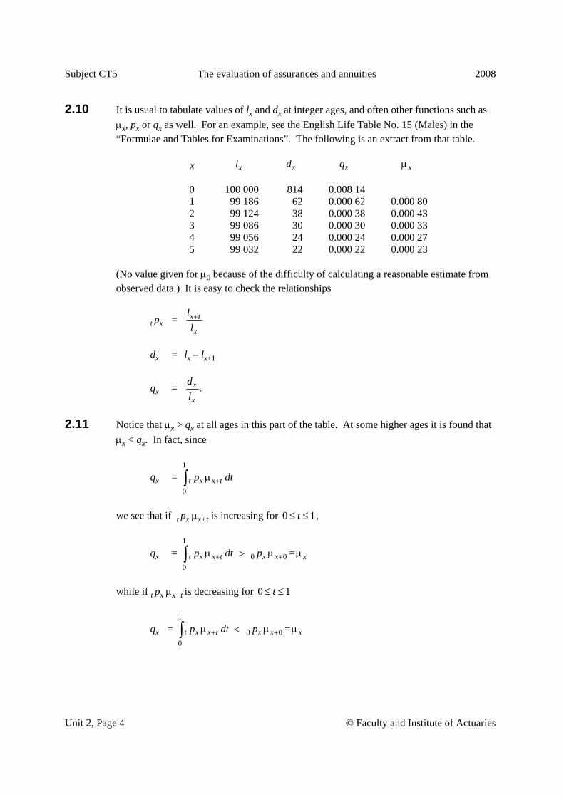
2.10 It is usual to tabulate values of lx and dx at integer ages, and often other functions such as μx, px or qx as well. For an example, see the English Life Table No. 15 (Males) in the “Formulae and Tables for Examinations”. The following is an extract from that table.
x xl xd xq xμ
0 100 000 814 0.008 14 1 99 186 62 0.000 62 0.000 80 2 99 124 38 0.000 38 0.000 43 3 99 086 30 0.000 30 0.000 33 4 99 056 24 0.000 24 0.000 27 5 99 032 22 0.000 22 0.000 23
(No value given for μ0 because of the difficulty of calculating a reasonable estimate from observed data.) It is easy to check the relationships
t px = x t
x
ll+
dx = lx – lx+1
qx = .x
x
dl
2.11 Notice that μx > qx at all ages in this part of the table. At some higher ages it is found that
μx < qx. In fact, since
qx = 1
0t x x tp dt+μ∫
we see that if t px μx+t is increasing for 0 1t≤ ≤ ,
qx = 1
0 00
=t x x t x x xp dt p+ +μ > μ μ∫
while if t px μx+t is decreasing for 0 1t≤ ≤
qx = 1
0 00
=t x x t x x xp dt p+ +μ < μ μ∫

2008 The evaluation of assurances and annuities Subject CT5
© Faculty and Institute of Actuaries Unit 2, Page 5
It is therefore of interest to note the behaviour of the function t px μx+t for 0 ≤ t < ω − x (recall that this function is the density of Tx). Figure 1 shows t p0 μt (i.e. the density of T = T0) for the English Life Table No. 15 (Males). It has the following features, which are typical of life tables based on human mortality in modern times.
Figure 1 f0(t) = t p0 μt (ELT15 (Males) Mortality Table) (1) Mortality just after birth (“infant mortality”) is very high. (2) Mortality falls during the first few years of life. (3) There is a distinct “hump” in the function at ages around 18–25. This is often
attributed to a rise in accidental deaths during young adulthood, and is called the “accident hump”.
(4) From middle age onwards there is a steep increase in mortality, reaching a peak at
about age 80. (5) The probability of death at higher ages falls again (even though qx continues to
increase) since the probabilities of surviving to these ages are small. 2.12 We will now introduce some more actuarial notation for probabilities of death, and give
formulae for them in terms of the life table lx. Define xn m q⏐ = P[n < Tx ≤ n + m]
0
0.01
0.02
0.03
0.04
0 20 40 60 80 100 120
Age t
f0(t)

Subject CT5 The evaluation of assurances and annuities 2008
Unit 2, Page 6 © Faculty and Institute of Actuaries
In words, xn m q⏐ is the probability that a life age x will survive for n years but die during
the subsequent m years. It is easy to see that
xn m q⏐ = x n x n m
x
l ll
+ + +−
or alternatively that xn m q⏐ = n px × m qx+n
2.13 An important special case for actuarial calculations is m = 1, since we often use
probabilities of death over one year of age. By convention, we drop the “m” and write 1 xn q⏐ = xn q⏐
It is easy to see that xn q⏐ = n px . qx+n = 1x n x n x n
x x
l l dl l
+ + + +−= .
2.14 Recall the definition of the curtate future lifetime, Kx. We now see that the probability
function of Kx can be written
P[Kx = k] = xk q⏐ .
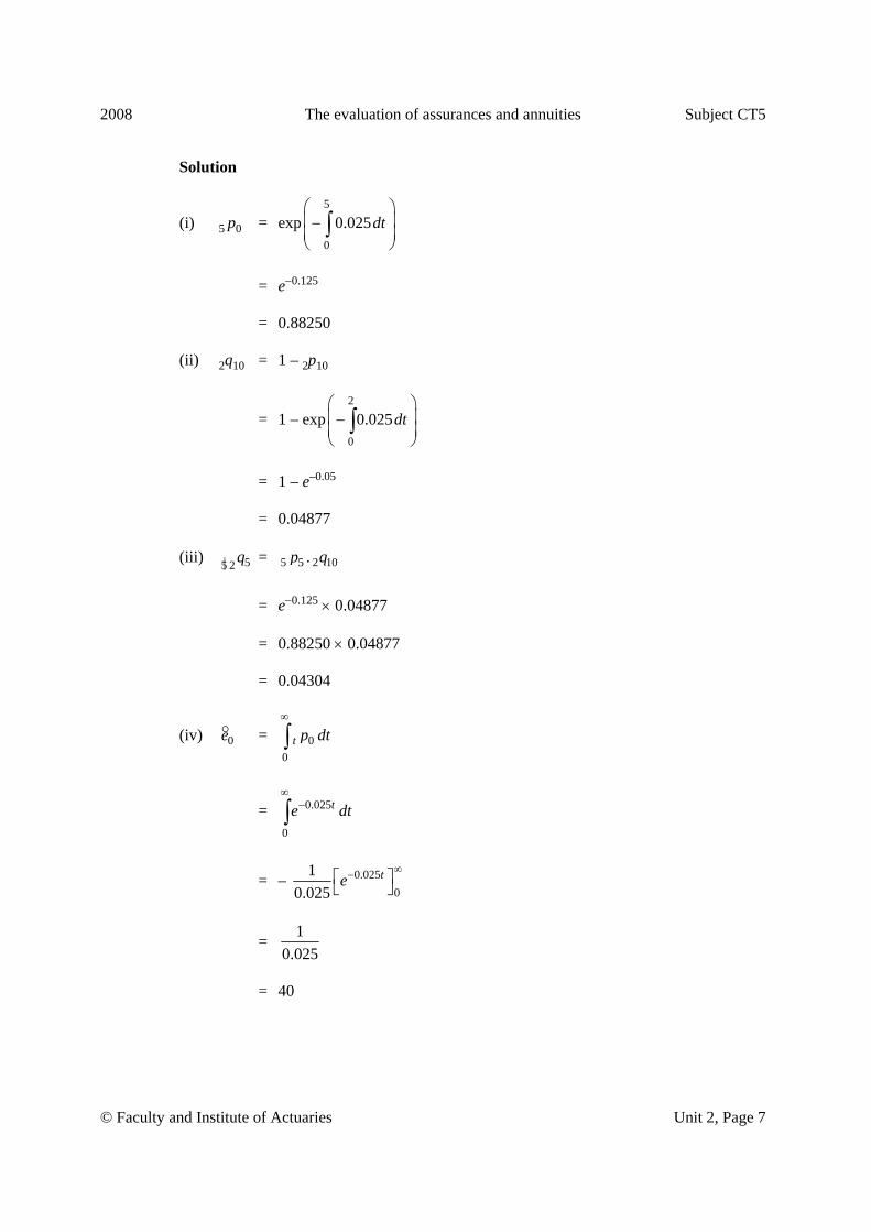
Example 1 In a certain population, the force of mortality equals 0.025 at all ages. Calculate: (i) the probability that a new-born baby will survive to age 5 (ii) the probability that a life aged exactly 10 will die before age 12 (iii) the probability that a life aged exactly 5 will die between ages 10 and 12 (iv) the complete expectation of life of a new-born baby (v) the curtate expectation of life of a new-born baby (Complete and curtate expectations of life, at age x, were defined in the Subject CT4,
Models.)
2008 The evaluation of assurances and annuities Subject CT5
© Faculty and Institute of Actuaries Unit 2, Page 7
Solution
(i) 5 p0 = exp5
0
0.025dt⎛ ⎞⎜ ⎟−⎜ ⎟⎝ ⎠∫
= e−0.125 = 0.88250 (ii) 2q10 = 1 – 2p10
= 1 – exp2
0
0.025dt⎛ ⎞⎜ ⎟−⎜ ⎟⎝ ⎠∫
= 1 – e–0.05 = 0.04877 (iii) 55 2 q⏐ = 5 5 2 10.p q
= e−0.125 × 0.04877 = 0.88250 × 0.04877 = 0.04304
(iv) 0e = 00
t p dt∞
∫
= 0.025
0
te dt∞
−∫
= – 0.0250
10.025
te∞−⎡ ⎤
⎣ ⎦
= 10.025
= 40

Subject CT5 The evaluation of assurances and annuities 2008
Unit 2, Page 8 © Faculty and Institute of Actuaries
(v) e0 = 01
kk
p∞
=∑
= 0.025
1
k
ke
∞−
=∑
= 0.025
0.0251e
e
−
−− = 39.5
3 Life table functions at non-integer ages 3.1 Life table functions such as lx, px or μx are usually tabulated at integer ages only, but
sometimes we need to compute probabilities involving non-integer ages or durations, such as 2.5p37.5. We can do so using approximate methods. We will show two methods.
3.2 In both cases, we suppose that we split up the required probability so that we need only
approximate over single years of age. For example, we would write 3p55.5 as 0.5p55.5 × 2p56 × 0.5p58. The middle factor can be found from the life table. To approximate the other two factors we need only consider single years of age.
3.3 The first method is based on the assumption that, for integer x and 0 ≤ t ≤ 1, the function
t px μx+t is a constant. Since this is the density of the time to death from age x, it is seen that this assumption is equivalent to a uniform distribution of the time to death, conditional on death falling between these two ages. Hence it is called the Uniform Distribution of Deaths (or UDD) assumption.
3.4 Since s qx = 0
s
t x x tp dt+μ∫ , by putting s = 1 we must have t px μx+t = qx (0 ≤ t ≤ 1) and
therefore
s qx = 0
. .s
x xq dt s q=∫
This is sometimes taken as the definition of the UDD assumption. Since qx can be found
from the life table, we can use this to approximate any s qx or s px (0 ≤ s ≤ 1).

2008 The evaluation of assurances and annuities Subject CT5
© Faculty and Institute of Actuaries Unit 2, Page 9
3.5 Note that we must have an integer age x in the above formula, so (in our example) we can now estimate 0.5 p58 but not 0.5 p55.5. It is easy to show that for 0 ≤ s < t ≤ 1,
( )1 .
xt s x s
x
t s qq
s q− +−
=−
[Hint: t px = s px × t–s px+s.] This result, with s = 0.5, t = 1, can be used to estimate
probabilities of the form 0.5 p55.5. 3.6 The second method of approximation is based on the assumption of a constant force of
mortality. That is, for integer x and 0 ≤ t < 1, we suppose that μx+t = μ = constant. Then the formula
0
=exp =t
tt x x sp ds e− μ
+
⎧ ⎫⎪ ⎪− μ⎨ ⎬⎪ ⎪⎩ ⎭∫
can be used to find the required probabilities. We first have to find μ. Note that px=e−μ so μ = – log px, which we can find from the life table. Next, note that matters are rather
simpler than under the UDD assumption since for 0 ≤ s < t < 1 we have
( )=exp =t
t st s x s x r
s
p dr e− − μ− + +
⎧ ⎫⎪ ⎪− μ⎨ ⎬⎪ ⎪⎩ ⎭∫
Hence we can easily calculate any required probability.
Subject CT5 The evaluation of assurances and annuities 2008
Unit 2, Page 10 © Faculty and Institute of Actuaries
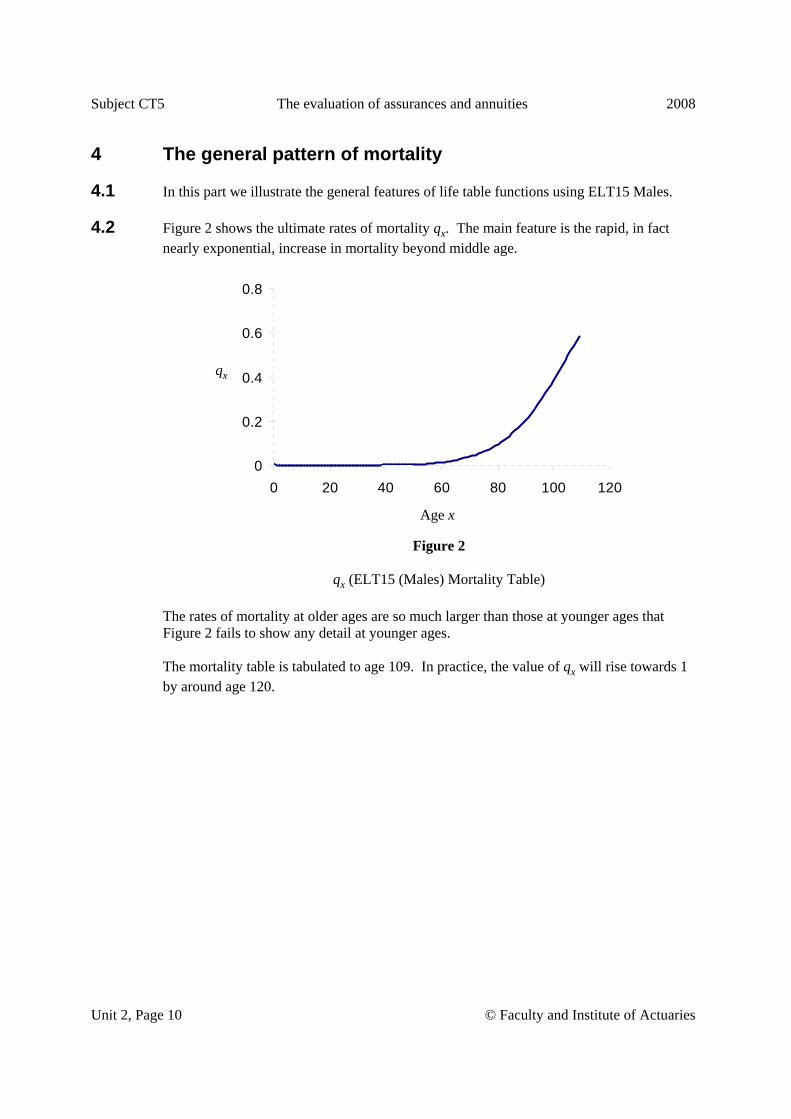
4 The general pattern of mortality
4.1 In this part we illustrate the general features of life table functions using ELT15 Males. 4.2 Figure 2 shows the ultimate rates of mortality qx. The main feature is the rapid, in fact
nearly exponential, increase in mortality beyond middle age.
Figure 2 qx (ELT15 (Males) Mortality Table) The rates of mortality at older ages are so much larger than those at younger ages that Figure 2 fails to show any detail at younger ages.
The mortality table is tabulated to age 109. In practice, the value of qx will rise towards 1 by around age 120.
0
0.2
0.4
0.6
0.8
0 20 40 60 80 100 120
qx
Age x

2008 The evaluation of assurances and annuities Subject CT5
© Faculty and Institute of Actuaries Unit 2, Page 11
4.3 Figure 3 shows qx on a vertical base 10 logarithmic scale.
Figure 3 qx on log10 scale (ELT15 (Males) Mortality Table) The main features are high infant mortality, an “accident hump” at ages around 20, and the nearly exponential increase at older ages. In practice, the graph would effectively reach 1 by age 120.
4.4 Figure 4 shows lx. The main feature is the very slight fall until late middle age, followed by a steep plunge.
Figure 4
lx (ELT15 (Males) Mortality Table)
0.0001
0.001
0.01
0.1
1
0 20 40 60 80 100 120
qx (log10 scale)
Age x
lx
Age x
0
20 000
40 000
60 000
80 000
100 000
120 000
0 20 40 60 80 100 120

Subject CT5 The evaluation of assurances and annuities 2008
Unit 2, Page 12 © Faculty and Institute of Actuaries
4.5 Figure 5 shows dx. Although the scale is different, this looks the same as Figure 1. The similarity is explained by the relationship
1
0
xx t x x t
x
dq p dt
l += = μ∫
Figure 5 dx (ELT15 (Males) Mortality Table)
5 Using the life table to evaluate means and variances
5.1 All of the formulae developed in Unit 1 (such as
Ax = 1
0
kk x
kv q
∞+
=∑
:x na = 1
0
nk
k xk
v p−
=∑ )
can (obviously) be evaluated by direct calculation given only the life table probabilities, and with the widespread use of computers this is often the simplest method.
5.2 To save the time involved in the direct calculation using the underlying probabilities, the gold “Formulae and Tables for Examinations” book tabulates a selection of annuity and assurance functions on certain interest rates (including higher interest rates for variance calculations) and various mortality tables.
0
1 000
2 000
3 000
4 000
0 20 40 60 80 100 120
Age x
dx
2008 The evaluation of assurances and annuities Subject CT5
© Faculty and Institute of Actuaries Unit 2, Page 13
For functions dependent upon age as well as term, tabulations are restricted in order to save space. For example, in AM92, :x na is tabulated for x + n = 60 and for x + n = 65.
Other values can be calculated using formulae like : = n
x n x x nx na a v p a +− .
Assurance functions may be calculated directly, or by calculation of a corresponding annuity value and then use of a formula like those laid out in Sections 3.2 and 3.3 of Unit 1.
5.3 When dealing with annuities paid continuously or with death benefits payable immediately on death, it is straightforward to calculate functions as above and use the relevant approximations for the type of insurance concerned. For example, for whole life contracts, the formulae would be ½x xa a≅ − ½(1 )x xA i A≅ +
5.4 Retrospective accumulations can be calculated along similar lines, so for example
:x ns =1
1(1 ) (1 ... )n nx x n x
x n
i l vp v pl
−−
+
+ + + +
= 1
1 1(1 ) (1 ) ... (1 )n nx x x n
x n
l i l i l il
−+ + −
+
+ + + + + + .
6 Evaluating means and variances without use of the life table
6.1 The main alternative to using a life table is to postulate a formula and parameter values for the probability t px in the equations of Unit 1 and then evaluate the expressions directly.
6.2 Equivalently a formula for t qx or μx+t could be postulated. 6.3 The difficulty of adopting this approach is that the postulation would need to be valid
across the whole age range for which the formulae might be applied. As can be seen from the discussion in Section 4 above, the shape of human mortality may make a simple postulation difficult. Simple formulae may, however, be more appropriate and expedient for non-life contingencies.

Subject CT5 The evaluation of assurances and annuities 2008
Unit 2, Page 14 © Faculty and Institute of Actuaries
7 Select mortality
7.1 Introduction
So far, we have made an assumption of ultimate mortality, that is, that mortality varies by age only. As discussed further in Unit 9 of this Subject, many other factors other than just age might affect observed mortality rates. In practice, therefore, the evaluation of assurance and annuity benefits is often modified to allow for other factors, than just age, which affect the survival probabilities. Many factors can be allowed for by segregating the population, the assumption being that an age pattern of mortality can be discerned in the sub-population. For example, a population may well be segregated by sex and then sex-specific mortality rates (and mortality tables) can be used directly by using the techniques so far described. Where, however, the pattern of mortality is assumed to depend not just on age, then slightly more complicated survival probabilities are employed. The most important, in the case of human mortality, is where the mortality rates depend upon duration as well as age, called select rates.
7.2 Mortality rates which depend on both age and duration
Select rates are usually studied by modelling the force of mortality μ as a function of the age at joining the population and the duration since joining the population. The usual notation is [x]+r age at date of transition [x] age at date of joining population
r duration from date of joining the population until date of transition and the transition intensity is written μ[x],r
l[x]+r number of lives alive at duration r having joined the population at age [x]
based on some assumed radix
In effect, a model showing how μ varies with r is constructed for each value of [x]. Instead of the single life age-specific life table described above we have a series of life tables, one for each value of [x].

2008 The evaluation of assurances and annuities Subject CT5
© Faculty and Institute of Actuaries Unit 2, Page 15
7.2.1 Displaying select rates
Once select rates have been estimated, it is conventional to display estimated rates for each age at entry into the population, [x], by age attained at the date of transition i.e. [x] + r. This can be done in an array . . . . . . . . . . . . . . . . . . . . . . . . . . . . . . . . . . . . . . . . . . . . . .
[ 1] 1 [ 2] 2 [ 3] 3[ ]
[ ] 1 [ 1] 2 [ 2] 3[ 1]
[ 1] 1 [ ] 2 [ 1] 3[ 2]
............................
............................
............................
x x xx
x x xx
x x xx
− + − + − +
+ − + − ++
+ + + − ++
μ μ μ μ
μ μ μ μ
μ μ μ μ
. . . . . . . . . . . . . . . . . . . . . . . . . . . . . . . . . . . . . . . . . . . . . . Each diagonal ( ) of the array represents a model of how rates vary with duration since joining the population for a particular age at the date of joining i.e. each is a set of life table mortality rates. The rates displayed on the rows of the array are rates for lives who have a common age attained at the time of transition, but different ages at the date of joining the population. If the rates did not depend on the duration since the date of joining the population, then apart from sampling error the rates on each row would be equal. Usually it is the case that rates depend on duration until duration s, and after s they are independent of duration. This phenomena is termed Temporary Initial Selection (see Unit 9) and s is called the length of the select period. In any investigation s is determined empirically by considering the statistical significance of the differences in transition rates along each row and the substantive impact of the different possible values of s. When a value of s has been determined, then the estimates of the rates for duration ≥ s are pooled to obtain a common estimated value which is used in all the life tables in which it is needed. The array can be written
. . . . . . . . . . . . . . . . . . . . . . . . . . . . . . . . . . . . . . . . . .
[ 1] 1 [ 2] 2 [ 1] 1[ ]
[ ] 1 [ 1] 2 [ 2] 1 1[ 1]
[ 1] 1 [ ] 2 [ 3] 1 2[ 2]
........
.........
............
x x x s s xx
x x x s s xx
x x x s s xx
− + − + − + + −
+ − + − + + − ++
+ + + − + + − ++
μ μ μ μ μ
μ μ μ μ μ
μ μ μ μ μ
. . . . . . . . . . . . . . . . . . . . . . . . . . . . . . . . . . . . . . . . . . and the pooled estimate at age attained x + s, for example, is given by
[ ], [ 1], 1 [ 2], 2
[ ], [ 1], 1 [ 2], 2
x s x s x sx s c c c
x s x s x sE E E− + − +
+− + − +
θ +θ +θμ =
+ +
……
……
Subject CT5 The evaluation of assurances and annuities 2008
Unit 2, Page 16 © Faculty and Institute of Actuaries
The right hand column of the above array represents a set of rates which are common to all the constituent life tables in the model of rates by age and duration. It is called an ultimate table. The initial select probabilities can be displayed in a similar way.
7.2.2 Constructing select and ultimate life tables
The first step in constructing life tables is to refine the crude estimated rates (μ or q) into a smooth set of rates which statistically represent the true underlying mortality rates. This refinement process, called “graduation”, is dealt with in Subject CT4, Models and we now assume that we have a set of graduated mortality rates. Using the graduated values of the initial probabilities displayed in the array . . . . . . . . . . . . . . . . . . . . . . . . . . . . . . . . . . . . . . . . . .
[ 1] 1 [ 2] 2 [ 1] 1[ ]
[ ] 1 [ 1] 2 [ 2] 1 1[ 1]
[ 1] 1 [ ] 2 [ 3] 1 2[ 2]
........
.........
............
x x x s s xx
x x x s s xx
x x x s s xx
q q q q q
q q q q q
q q q q q
− + − + − + + −
+ − + − + + − ++
+ + + − + + − ++
. . . . . . . . . . . . . . . . . . . . . . . . . . . . . . . . . . . . . . . . . . a table representing the select and ultimate experience can be constructed. This is achieved by firstly constructing the ultimate life table based on the final column of the array and the formulae described in part 2 above: • choose the starting age of the table, k • choose an arbitrary radix for the table, k
• recursively calculate the values of x using 1x+ = x (1 – qx) Beginning with the appropriate ultimate value in the final column the select life table functions for each row of the array are determined. This is achieved by “working backwards” up each diagonal using
[ ] 1[ ]
[ ]1x t
x tx tq+ +
++
=−
for t = s −1, …, 1, 0

2008 The evaluation of assurances and annuities Subject CT5
© Faculty and Institute of Actuaries Unit 2, Page 17
and noting in the first iteration that [ ] 1 1x s+ − + = x s+
7.2.3 Using tabulated select life table functions
Some probabilities are particularly useful for life contingencies calculations. We have already defined
| = x n x n mn m x
xq + + +−
1| = x n x n
n xx
q + + +−
representing the m year and 1 year transition probabilities when the event of transition is deferred for n years. Similar probabilities can be defined for each select mortality table
[ ] [ ]| [ ]
[ ]= x r n x r n m
n m x rx r
q + + + + ++
+
−
[ ] [ ] 1| [ ]
[ ]= x r n x r n
n x rx r
q + + + + ++
+
−
with the special case of n = 0 and m = n being of particular interest
[ ] [ ][ ]
[ ]= x r x r n
n x rx r
q + + ++
+
−
and the complement of this n year transition probability, the n year survival probability is
[ ][ ]
[ ]= x r n
n x rx r
p + ++
+.
The above probabilities may also be expressed in terms of the number of deaths in the select mortality table by defining
d[x]+r = l[x]+r − l[x]+r+1.
Subject CT5 The evaluation of assurances and annuities 2008
Unit 2, Page 18 © Faculty and Institute of Actuaries
7.2.4 Evaluating means and variances using select mortality
Corresponding to the assurances and annuities defined in Unit 1 are select equivalents defined as before but assumed to be issued to a select life denoted [x] rather than x.
So, for example, 1[ ] | [ ]
0=
kk
x k xk
A v q=∞
+
=∑ can be used to calculate the EPV of benefits of a
whole life assurance issued to a select life aged [x] at entry.
Similarly, [ ] [ ]0
= .k
kx k x
ka p v
=∞
=∑ can be used to calculate the EPV of benefits of a whole life
annuity-due, with level annual payments, issued to a select life aged [x] at entry. The variance formulae established in Unit 1 also apply replacing x with [x], as do the relationships in Section 3.2 of Unit 1, namely that:
A[x] = [ ]1 xda− and
[ ]: [ ]:= 1x n x nA da−
E N D

2008 Net premiums and reserves Subject CT5
© Faculty and Institute of Actuaries Unit 3, Page 1
UNIT 3 — NET PREMIUMS AND RESERVES
Syllabus objective (iii) Describe and calculate, using ultimate or select mortality, net premiums and net
premium reserves of simple insurance contracts. 1. Define the net random future loss under an insurance contract, and state the
principle of equivalence. 2. Define and calculate net premiums for the insurance contract benefits in
objective (i) 1. Premiums and annuities may be payable annually, more frequently than annually, or continuously. Benefits may be payable at the end of the year of death, immediately on death, annually, more frequently than annually, or continuously.
3. State why an insurance company will set up reserves. 4. Describe prospective and retrospective reserves. 5. Define and evaluate prospective and retrospective net premium reserves in
respect of the contracts in objective (i) 1., with premiums as in (iii) 2. 6. Show that prospective and retrospective reserves are equal when calculated on
the same basis. 7. Derive recursive relationships between net premium reserves at annual
intervals, for contracts with death benefits paid at the end of the year of death, and annual premiums.
8. Derive Thiele’s differential equation, satisfied by net premium reserves for
contracts with death benefits paid at the moment of death, and premiums payable continuously.
9. Define and calculate, for a single policy or a portfolio of policies (as
appropriate):
• death strain at risk • expected death strain • actual death strain • mortality profit

Subject CT5 Net premiums and reserves 2008
Unit 3, Page 2 © Faculty and Institute of Actuaries
1 Equations of value
1.1 Definition In Subject CT1, Financial Mathematics payments were generally treated as certain to be paid. The equation of value where payments are certain has already been introduced there. In most actuarial contexts some or all of the cash flows in a contract are uncertain, depending on the death or survival (or possibly the state of health) of a life. We therefore extend the concept of the equation of value to deal with this uncertainty, by equating expected present values of uncertain cashflows. The equation of expected present values for a contract, usually referred to as the equation of value, is
The expected present value of the income = The expected present value of the outgo
Alternatively, this is referred to as the principle of equivalence.
1.2 The income to a life insurer comes from the payments made by policyholders, called the premiums. The outgo arises from benefits paid to policyholders and expenses of the insurer. Given a suitable set of assumptions, which we call the basis, we may use the equation of value to calculate the premium or premiums which a policyholder must make in return for a given benefit. We may also calculate the amount of benefit payable for a given premium.
1.3 We may also use the equation of value when a policyholder wishes to adjust the terms of a
contract after it is effected — for example by changing the contract term. 1.4 In the remainder of this Unit we will concentrate on net premiums and the associated net
premium reserves (i.e. we will ignore actual premiums and the associated gross premium reserves). Although the relevance of the net premium valuation in the UK has diminished in recent years, primarily on account of regulatory changes, it continues to play a significant role in territories other than the UK and therefore remains an important part of this Subject. Gross premium valuations, on which much greater emphasis is now placed in the UK, are covered in Unit 5.
2 The basis 2.1 The basis for applying the equation of value for a life insurance contract will specify the
mortality and interest rates to be assumed.

2008 Net premiums and reserves Subject CT5
© Faculty and Institute of Actuaries Unit 3, Page 3
2.2 Usually the assumptions will not be the best estimates we can find of the individual basis elements, but will be more cautious than the best estimates. For example, if we expect to earn a rate of interest of 8% p.a. on the invested premiums, we may calculate the premiums assuming we earn only 6% p.a. As we are assuming that we earn less interest than we really expect, then the premiums calculated will be higher than they would need to be if the expected rate of 8% were actually earned. Some reasons for this element of caution in the basis are: 1. To allow a contingency margin, to ensure a high probability that the premiums plus
interest income meet the cost of benefits allowing for random variation. In other words to ensure a high probability of making a profit.
2. To allow for uncertainty in the estimates themselves.
3 Premiums 3.1 The premium payment arrangement will commonly be one of the following:
• A single premium contract, under which benefits are paid for by a single lump sum
premium paid at the time the contract is effected. This payment is certain, so that the left hand side of the equation of value is the certain payment, not the expected value of a payment.
• An annual premium contract, under which benefits are paid for by a regular annual
payment of a level amount, the first premium being due at the time the contract is effected. Premiums continue to be paid in advance until the end of some agreed maximum premium term, often the same as the contract term, or until the life dies if this is sooner. Therefore, there would not usually be a premium paid at the end of the contract term.
• A true mthly premium contract, under which benefits are paid for by m level
payments made every 1/m years. As in the annual premium case, premiums continue to be paid in advance until the end of some agreed maximum premium term or until the life dies if this is sooner. Again, there would not usually be a premium paid at the end of the contract term. Often the premium is paid monthly (that is, m = 12). For some types of contract, weekly premiums are possible.
3.2 Premiums are always paid in advance, so the first payment is always due at the time the
policy is effected. 3.3 Given a basis specifying mortality and interest to be assumed, and given details of the
benefits to be purchased, we can use the equation of value to calculate the premium payable.

Subject CT5 Net premiums and reserves 2008
Unit 3, Page 4 © Faculty and Institute of Actuaries
4 The net premium
4.1 Definition The net premium is the amount of premium required to meet the expected cost of the
assurance or annuity benefits under a contract, given mortality and interest assumptions. The net premium is also sometimes referred to as the pure premium or the risk premium.
4.2 The net premium for a contract, given suitable mortality and interest assumptions, is found from the equation of expected present value:
The expected present value of the net premium income = The expected present value of the outgo on benefits
4.3 Notation We have some standard notation for the net premiums of common life insurance contracts,
related to the notation for the expected present value of the assurance benefits which the net premium is to pay for:
4.3.1 :x nP is the net premium payable annually in advance throughout the duration of the
contract for an endowment assurance issued to a life aged x with term n years, under which the sum assured is 1, payable at the end of the year of death or at maturity, where ultimate mortality is assumed. From the net premium definition:
::
:
= x nx n
x n
AP
a
If the death benefit is instead payable immediately on death then the net premium payable annually in advance is denoted by :( )x nP A and
::
:
( ) = x nx n
x n
AP A
a

2008 Net premiums and reserves Subject CT5
© Faculty and Institute of Actuaries Unit 3, Page 5
If the premium is instead payable m-thly per annum in advance, this would be denoted by placing a superscript (m) above the P and a functions. So, assuming again that the death benefit is payable at the end of the year of death, for example, we would have
( ) :( )::
=m x nmx n
x n
AP
a
If the premium is payable continuously then, assuming again that the death benefit is payable at the end of the year of death, for example, we would have :x nP and
::
:
= x nx n
x n
AP
a
The final main variation would be to assume select, rather than ultimate, mortality. Then the above expressions apply but with x replaced by [x].
[ ]:x nP
is the net premium payable annually in advance throughout the duration of the contract for an endowment assurance issued to a life aged x with term n years, under which the sum assured is 1, payable at the end of the year of death or at maturity, where select mortality is assumed.
[ ]:x nP = [ ]:
[ ]:
x n
x n
A
a
The above notation is flexible enough for the relevant symbols to be unambiguously combined in different ways when the benefits and premiums have alternative combinations of timings to those shown above. A full description of the approach to this notation can be found, for example, in the “International Notation Section” of the “Formulae and Tables for Examinations”.
Without loss of generality, we now show the corresponding notation for other simple insurance contracts assuming ultimate mortality, annual premiums in advance, and death benefits payable at the end of the year of death. We leave it to the reader to provide the alternative combinations in a similar manner to those outlined above.
Subject CT5 Net premiums and reserves 2008
Unit 3, Page 6 © Faculty and Institute of Actuaries
4.3.2 1:x nP is the net premium payable annually in advance throughout the duration of the
contract for a term assurance issued to a life aged x with term n years, under which the sum assured is 1, payable at the end of the year of death, and where ultimate mortality is assumed. From the net premium definition:
1:1
::
= x nx n
x n
AP
a
4.3.3 Px is the net premium payable annually in advance throughout the duration of the contract
for a whole life assurance issued to a life aged x, under which the sum assured is 1, payable at the end of the year of death, and where ultimate mortality is assumed.
From the net premium definition:
= xx
x
AP
a
4.3.4 t Px is the net premium payable annually in advance for a maximum of t years (or until
earlier death) for a whole life assurance issued to a life aged x, under which the sum assured is 1, payable at the end of the year of death, and where ultimate mortality is assumed. From the net premium definition:
t Px = :
x
x t
Aa
4.3.5 There is no agreed notation for premiums payable on a critical illness assurance.
5 Reserves
5.1 Prospective reserve The prospective reserve for a life insurance contract which is in force (that is, has been written but has not yet expired through claim or reaching the end of the term) is defined to be, for a given basis:
The expected present value of the future outgo − The expected present value of the future income

2008 Net premiums and reserves Subject CT5
© Faculty and Institute of Actuaries Unit 3, Page 7
This is the prospective reserve because it looks forward to the future cashflows of the contract. The prospective reserve is important because if the office holds funds equal to the reserve, and the future experience follows the reserve basis, then, averaging over many policies, the combination of reserve and future income will be sufficient to pay the future liabilities. The reserve therefore gives the office a measure of the minimum funds it needs to hold at any point during the term of a contract. The process of calculating a reserve is called the valuation of the policy.
5.2 Another view of the prospective reserve is gained by considering the net random future loss (or just “net loss”) from a policy which is in force — where the net loss, L, is defined to be:
L = present value of the future outgo − present value of the future income
Now L is a random variable, since both terms are random variables which depend on the policyholder's future lifetime. (If premiums are not being paid, the second term is zero, the first term is a random variable, so L is still a random variable). The reserve may now be defined as
Prospective Reserve = E[L]
5.3 Why hold reserves? In many life insurance contracts, the expected cost of paying benefits increases over the term of the contract — consider an endowment assurance, for example. The probability that the benefit will be paid in the first few years is small — the life is young and in good health. Later the expected cost increases as the life ages and the probability of a claim by death increases. In the final year the probability of payment is large, since the payment will be made if the life survives the term, and for most contracts (which often mature when the policyholder is in his or her 50s or 60s) the probability of survival is large. Although on average the cost of the benefit is increasing over the term, the premiums which pay for these benefits are level. This means that the premiums received in the early years of a contract are more than enough to pay the benefits that fall due in those early years, but that in the later years, and particularly in the last year of an endowment assurance policy, the premiums are too small to pay for the benefits. It is therefore prudent for the premiums which are not required in the early years of a contract to be set aside, or provisioned, to fund the shortfall in the later years of the contract. While funds are provisioned, they are invested so that interest also contributes to the cost of benefits. If the life insurance company was to spend all the premiums received, perhaps by distributing to shareholders the premiums that were not required to pay benefits, then later in the contract the company may not be able to find the money to pay for the excess of the cost of benefits over the premiums received. We set up reserves to ensure (as far as possible) that this does not happen, and that the office remains solvent.

Subject CT5 Net premiums and reserves 2008
Unit 3, Page 8 © Faculty and Institute of Actuaries
5.4 Retrospective reserves The retrospective reserve for a life insurance contract which is in force is defined to be, for a given basis:
The accumulated value allowing for interest and survivorship of the premiums received to date − the accumulated value allowing for interest and survivorship of the benefits and expenses paid to date
The accumulated value of benefits, sometimes called the cost of assurance, for a life who purchased a life insurance policy at age x, and is now age x + t, where the sum assured for the t years of past cover was S, payable at the end of the year of death, is
1: (1 ) .t x
x tx t
SA i+
+
The accumulated premiums for the life, assuming premiums of P per annum payable annually in advance, is:
: :(1 ) =t xx t x t
x tPa i PS
++
The retrospective reserve on a given basis tells us how much the premiums less claims have accumulated to, averaging over a large number of policies.
5.5 Conditions for equality of prospective and retrospective
reserves If: 1. the retrospective and prospective reserves are calculated on the same basis, and 2. this basis is the same as the basis used to calculate the premiums used in the reserve
calculation, then the retrospective reserve will be equal to the prospective reserve.
5.6 In practice these conditions rarely hold, since the assumptions which are appropriate for the retrospective calculation (for which we use the experienced conditions over the duration of the contract up to the valuation date) are not generally appropriate for the prospective calculation, which will use assumptions considered suitable for the remainder of the policy term. Also, the assumptions which were considered appropriate at the time the premium was calculated may not be appropriate for the retrospective or prospective reserve some years later.

2008 Net premiums and reserves Subject CT5
© Faculty and Institute of Actuaries Unit 3, Page 9
We demonstrate the equality with an example, tVx , the reserve at duration t years for a whole life assurance to a life age x, assuming death benefits payable at the end of the year and ultimate mortality. The prospective reserve is: Ax+t − x x tP a + and the retrospective reserve is:
1: :
(1 )t
x t x txt x
iP s Ap+
− .
The first term in the retrospective reserve is interpreted as the expected accumulation of premiums received, and the second term as the expected accumulated cost of benefits paid. Start with the prospective reserve: tVx = Ax+t − Px x ta + = Ax+t − Px : :x t x tx t x xa P s P s+ − +
Now t⏐ax = vt t px x ta + , and :x ts = :(1 )t
x tt x
i ap+
∴ t Vx = :(1 )t
x txt x
iP sp+
− Px (t⏐ax + : )x ta + Ax+t
= :(1 )t
x txt x
iP sp+
− Px xa + Ax+t
= :(1 )t
x txt x
iP sp+
− Ax + Ax+t
= :(1 )t
x txt x
iP sp+
− 1:x tA
The details of this proof can easily be adjusted for other types of contract.
5.7 Reserve conventions We often calculate reserves at integer durations. In this case, we calculate the reserve just before any payment of premium due on that date, and just after any payment of annuity payable in arrear due on that date. The general rule is, for valuation on the tth policy anniversary, payments in respect of the year t − 1 to t payable in arrear (i.e. on the tth
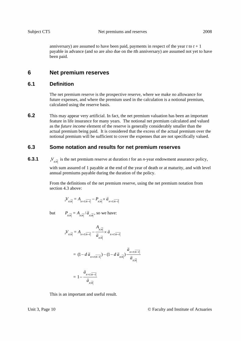
Subject CT5 Net premiums and reserves 2008
Unit 3, Page 10 © Faculty and Institute of Actuaries
anniversary) are assumed to have been paid, payments in respect of the year t to t + 1 payable in advance (and so are also due on the tth anniversary) are assumed not yet to have been paid.
6 Net premium reserves
6.1 Definition
The net premium reserve is the prospective reserve, where we make no allowance for future expenses, and where the premium used in the calculation is a notional premium, calculated using the reserve basis.
6.2 This may appear very artificial. In fact, the net premium valuation has been an important feature in life insurance for many years. The notional net premium calculated and valued as the future income element of the reserve is generally considerably smaller than the actual premium being paid. It is considered that the excess of the actual premium over the notional premium will be sufficient to cover the expenses that are not specifically valued.
6.3 Some notation and results for net premium reserves
6.3.1 :t x nV is the net premium reserve at duration t for an n-year endowment assurance policy,
with sum assured of 1 payable at the end of the year of death or at maturity, and with level annual premiums payable during the duration of the policy. From the definitions of the net premium reserve, using the net premium notation from section 4.3 above: : : : :=t x n x t n t x n x t n tV A P a
+ − + −− ×
but : : := /x n x n x nP A a , so we have:
:: : :
:
= x nt x n x t n t x t n t
x n
AV A a
a+ − + −− ×
= :: :
:
(1 ) (1 ) x t n tx t n t x n
x n
ad a d a
a+ −
+ −− − −
= :
:
1 x t n t
x n
a
a+ −
−
This is an important and useful result.

2008 Net premiums and reserves Subject CT5
© Faculty and Institute of Actuaries Unit 3, Page 11
6.3.2 We find a similar result for tVx, the net premium reserve at duration t of an annual premium whole life assurance, issued to a life aged x, with premiums payable throughout the contract, and with the sum assured payable at the end of the year of death: tVx = x t x x tA P a+ +−
= xx t x t
x
AA aa+ +−
= (1 ) (1 ) x tx t x
x
ad a d a
a+
+− − −
= 1 x t
x
aa
+−
6.3.3 In the continuous time case, the corresponding definition and relationships are, for
endowment assurances:
:x ntV = E[L] = : : :x t n t x n x t n tA P a+ − + −− = 1 − :
:
x t n t
x n
a
a+ −
and for whole life assurances:
t xV = E[L] = x t x x tA P a+ +− = 1 − x t
x
aa
+ .
We leave the proofs to the reader. 6.3.4 In m-thly premium cases, such straightforward equalities as given in 6.3.3 would not hold
and reserves would need to be calculated from the basic formulae.
The notation for such reserves follows the notation approach described above in Section 4.3. The provision, for a unit benefit, is denoted V and subscripts and superscripts may be added. The right subscript corresponds to the subscript of the assurance benefit function for the contract; the right superscript (if any) indicates the premium frequency per annum of the contract; the left subscript indicates the duration at which the reserve is taken. Hence, for example, ( )1
:m
t x nV is the net premium reserve at duration t of an n-year pure
endowment, sum assured 1, premiums payable mthly.

Subject CT5 Net premiums and reserves 2008
Unit 3, Page 12 © Faculty and Institute of Actuaries
The provision calculation, for a whole life assurance payable by true monthly premiums and assuming a benefit paid at the end of the year of death, for example, at integral duration t would be based on the formula
( ) ( ) ( )=m m m
t x x t x x tV A P a+ +−
which could be evaluated using the mthly annuity approximation ( ) 12
mx t x
ma am+−
≅ − .
6.3.5 1
:t x nV is the net premium reserve at duration t for an n-year term assurance policy, with
sum assured of 1 payable at the end of the year of death, and with level annual premiums payable during the duration of the policy. This may be evaluated from first principles as 1 1 1
: : : :=t x n x t n t x n x t n tV A P a+ + + −
−
and there is no neat simplification as in the whole life and endowment assurance cases.
6.3.6 Note that it is easy to show that: 1 1
: : :=t t tx n x n x nV V V+
6.3.7 The above discussion can be simply extended to annuity, rather than assurance contracts.
6.3.8 The above discussion can be applied to a critical illness assurance by replacing the
probabilities of death with the probabilities of being diagnosed from any of the critical illnesses covered by the policy.
7 Recursive calculation of reserves 7.1 Conditions for recursive calculations
We will develop relationships between the reserves at successive integer durations for net premium reserves. For these relationships to hold, the reserves at successive durations and the net premiums must be calculated on the same basis.
7.2 Net premium reserves at successive durations
Let i be the valuation interest rate, and let qy and py be the valuation rates of mortality and survival at age y.

2008 Net premiums and reserves Subject CT5
© Faculty and Institute of Actuaries Unit 3, Page 13
7.2.1 Whole life assurance
With sum assured 1 payable at the end of the year of death, annual premiums: (tVx + Px)(1 + i) = qx+t + px+t .t+1Vx Proof (tVx + Px) = (Ax+t − Px äx+t) + Px but Ax+t = vqx+t + vpx+tAx+t+1 and äx+t = 1 + vpx+t äx+t+1 so (tVx + Px) = vqx+t + vpx+tAx+t+1 − Px (1 + vpx+täx+t+1) + Px = v(qx+t + px+t (Ax+t+1 − Px äx+t+1)) = v(qx+t + px+t.t+1Vx) ⇒ (tVx + Px) (1 + i) = qx+t + px+t.t+1Vx
7.2.2 General reasoning It is very helpful to consider a verbal explanation of this result. If the insurer holds reserves at the start of the year equal to the policy reserve, then the total at the year end of the reserve brought forward, plus the premium income, plus the interest earned on these, must be equal to the expected cost of the death benefits at the year end (here the benefit is 1 payable with probability qx+t) plus the expected cost of setting up the reserve at the year end of the year end reserve (here the reserve of t+1Vx is required with probability px+t). In the case above, the relationship states that the year end value of the policy income for the year equals the expected value of the policy outgo at the year end. If the income were a random variable (for example, if the premiums were payable mthly, so that payment depended on survival), then the relationship would be that the expected income, accumulated to the year end, is equal to the expected value of the year end outgo.
Subject CT5 Net premiums and reserves 2008
Unit 3, Page 14 © Faculty and Institute of Actuaries
7.2.3 Further examples
Some further relationships are given. It is left to the reader to verify these.
( ) 1: : :(1 )t x t x t tx n x n x nV P i q p V+ + ++ + = + (1)
( )1 1 11: : :(1 )t x t x t tx n x n x nV P i q p V+ + ++ + = + (2)
( )1 1 11: : :(1 )t x t tx n x n x nV P i p V+ ++ + = (3)
8 Mortality profit
8.1 In the last section it was shown that, if the experience exactly follows the reserve basis, then, on average, the income and outgo in each policy year are equal. If the experience does not follow the assumptions then there will either be an excess of income over outgo (a profit, or surplus) or an excess of outgo over income (a loss or negative profit). Profits and losses may arise from any element of the reserve basis. For example: 1. If the interest earned is greater than that assumed in the reserve, then the income will
accumulate to more than the sum required to cover the cost of the benefits and the year end reserve, giving an interest surplus.
2. If the policyholder decides to surrender his or her policy (that is, to cease paying
premiums, and take some lump sum in respect of the future benefits already paid for) then the year end outgo is not as assumed. The lump sum will be required in place of the year end reserve and there will be a surrender profit (positive if the lump sum is less than the reserve).
3. If the experienced mortality is heavier than that assumed in the basis, then there will
be a profit or loss from mortality.
8.2 We consider here mortality profit only. We assume, therefore, that in all elements other than mortality, experienced rates follow the assumed rates exactly.
2008 Net premiums and reserves Subject CT5
© Faculty and Institute of Actuaries Unit 3, Page 15
8.3 Death strain at risk (DSAR)
Consider a policy issued t years ago to a life then aged x, with sum assured of S payable at the end of the year of death. Also, assume that no survival benefit is due if the life survives to t + 1 (we will extend the ideas to survival benefits in a later section). Let tV be the reserve at time t. Then we define the death strain in the policy year t to t + 1 to be the random variable, DS, say, DS = 0 if the life survives to t + 1 = (S − t+1V) if the life dies in the year t → t + 1 The maximum death strain, (S − t+1V) is called the death strain at risk or DSAR. The word strain is used loosely to mean a cost to the office. The reasoning behind the DSAR definition is seen more clearly if we rearrange the recursive relationship between tV and t+1V, assuming level premiums for simplicity: (tV + P)(1 + i) = qx+t S + px+t.t+1V = qx+t S + (1 − qx+t) t+1V = t+1V + qx+t (S − t+1V) In words, the reasoning is that for each policy we must pay out at least t+1V at the end of the year. In addition, if the policy becomes a claim during the year, with probability qx+t, then we must pay out an extra sum of (S − t+1V) which is the DSAR. Note that qx+t is the probability of dying in the year t to t + 1, and therefore x + t is the age at the start of the year.
8.4 Expected death strain (EDS)
The expected amount of the death strain is called the expected death strain (EDS).This is the amount that the life insurance company expects to pay extra to the year end reserve for the policy. The probability of claiming in the policy year t to t + 1 is qx+t so that: EDS = qx+t (S − t+1V)
8.5 Actual death strain (ADS)
The actual death strain is simply the observed value at t + 1 of the death strain random variable, that is, ADS = 0 if the life survived to t + 1 = (S − t+1V) if the life died in the year t → t + 1

Subject CT5 Net premiums and reserves 2008
Unit 3, Page 16 © Faculty and Institute of Actuaries
8.6 Mortality profit
The mortality profit is defined as:
Mortality Profit = Expected Death Strain − Actual Death Strain The EDS is the amount the company expects to pay out, in addition to the year end reserve for a policy. The ADS is the amount it actually pays out, in addition to the year- end reserve. If it actually pays out less than it expected to pay, there will be a profit. If the actual strain is greater than the expected strain there will be a loss.
8.7 Mortality profit on a portfolio of policies
We are often interested in analysing the experience of a group of similar policies. We use the term portfolio of policies to mean any group of policies. In this case we simply sum the EDS and the ADS over all the relevant policies. If all lives are the same age, and subject to the same mortality table, this gives: Total DSAR = 1
all policies( )tS V+−∑
Total EDS = 1
all policies( )x t tq S V+ +−∑
= 1all policies
( )x t tq S V+ +
⎛ ⎞⎜ ⎟−⎜ ⎟⎝ ⎠
∑
= qx+t DSAR Total ADS = 1
death claims( )tS V+−∑
Mortality Profit = EDS − ADS In many situations the DSAR of each of the individual policies is not known, but the total DSAR is simply the total sum assured less the total year end reserve, and the EDS is qx+t DSAR.
8.8 Allowing for survival benefits
8.8.1 Suppose the contract provides for a benefit at the end of a policy year t to t + 1. By convention, the present value of this will have been included in tV but will fall outside the computation of t+1V. So, the survival benefit needs to be allowed for as an additional payment from the reserve.

2008 Net premiums and reserves Subject CT5
© Faculty and Institute of Actuaries Unit 3, Page 17
8.8.2 Let R be the benefit payable at the end of the policy year t → t + 1 contingent on the survival of the policyholder. The recursive relationship between successive reserves is now: (tV + P)(1 + i) = qx+t S + px+t (t+1V + R) = qx+t S + (1 − qx+t) (t+1V + R) = t+1V + R + qx+t (S − (t+1V + R)) The DS is now: DS = 0 if the life survives to t + 1 = S − (t+1V + R) if the life dies in the year t → t + 1 as the office must pay out (t+1V + R) for all policyholders, and an additional S − (t+1V + R) for policies becoming claims by death. The expected death strain is then qx+t (S − (t+1V + R)); the actual death strain is 0 if the life survived the year and (S − (t+1V + R)) if the life died during the year; the mortality profit is EDS − ADS.
8.8.3 In the case of an annuity of R p.a., payable annually in arrear, with no death benefit, the DSAR would be −(t+1V + R) (so each death causes a negative strain or release of reserves).
9 Thiele’s differential equation 9.1 In Section 7, we developed a recursive scheme which governs the development of the
reserve from one year to the next. With a little rearrangement, this can be written as a difference equation. For example, the recursion in Section 7.2.1 can be written:
t+1Vx − tVx = 1
x tp + {i . tVx + (1 + i) Px − qx+t (1 −tVx)}.
9.2 If we work in continuous time, we get instead a differential equation, called Thiele’s
differential equation. Suppose that:
(a) interest is earned continuously at force of interest δ (b) premiums are payable continuously at rate xP per annum; and (c) the sum assured of 1 is payable immediately on death

Subject CT5 Net premiums and reserves 2008
Unit 3, Page 18 © Faculty and Institute of Actuaries
Then it is easily seen that, over a short time period dt, the above equation becomes: t dt x t xV V+ − = { . (1 ) } ( )t x x t x x tV dt P dt V dt o dt+δ + − − μ + or, dividing by dt and taking limits:
t xVt
∂∂
= (1 ) .t x x t x x tV P V +δ + − − μ
This is Thiele’s equation for this type of policy.
9.3 There is a version of Thiele’s equation for each different type of contract. 9.4 The explanation above just shows the link between the difference equation we have
already used in discrete time, and the corresponding differential equation in continuous time. It is not an adequate derivation of Thiele’s equation. That can be provided in several ways. For example, we know that
t xV = x t x x tA P a+ +−
= 1 − x t
x
aa
+
Differentiating x ta + directly, we get
x tat +
∂∂
= 0
ss x te p ds
t
∞−δ
+∂∂ ∫
= 0
ss x te p ds
t
∞−δ
+∂∂∫
= 0
se∞
−δ∫ s px+t (μx+t − μx+t+s) ds
= μx+t x t x ta A+ +−

2008 Net premiums and reserves Subject CT5
© Faculty and Institute of Actuaries Unit 3, Page 19
Hence t
∂∂
t xV = x t x t x t
x
a Aa
+ + +−μ +
= − μx+t (1 − t xV ) + (1 )x t
x
aa
+− δ
= − (1 − t xV ) μx+t + 11 x t
x x
aa a
+⎛ ⎞δ − − δ +⎜ ⎟
⎝ ⎠
= − (1 − t xV ) μx+t + δ t xV + 1 x
x
aa
− δ
= − (1 − t xV ) μx+t + δ t xV + xP This is Thiele’s equation for a whole life assurance contract.
9.5 Note that Thiele’s equation, like the difference equation for reserves in discrete time, requires that the premium xP be calculated on the same basis as the reserves themselves.
E N D


2008 Variable benefits and annuities Subject CT5
© Faculty and Institute of Actuaries Unit 4, Page 1
UNIT 4 — VARIABLE BENEFITS AND ANNUITIES Syllabus objective (iv) Describe the calculation, using ultimate or select mortality, of net premiums and net
premium reserves for increasing and decreasing benefits and annuities. 1. Extend the techniques of (ii) to calculate the expected present value of an
annuity, premium, or benefit payable on death, which increases or decreases by a constant compound rate. Calculate net premiums and net premium reserves for contracts with premiums and benefits which vary as described.
2. Define the symbols (IA)x , ( )xIa , and (Ia)x and their select equivalents. 3. Calculate the expected present value of an annuity, premium or benefit payable
on death, which increases or decreases by a constant monetary amount. Calculate net premiums and net premium reserves for contracts with premiums and benefits which vary as described.
4. Define with profits contract. 5. List the types of bonus that may be given to with profits contracts. 6. Calculate net premiums and net premium reserves for with profits contracts.
1 Variable payments
1.1 The simple contracts discussed so far have had constant payments of the form: • a benefit of 1 payable on death; or • a benefit of 1 payable, at some frequency, on survival to the date of payment
1.2 We consider now the possibility that the payment amount varies. In the case of a benefit payable on death, let the payment be Yx if death occurs in the year of age (x, x + 1). Assume first that the benefit is payable at the end of the year of death. The EPV of this death benefit, to a life currently aged x, will be given by, using life table notation,
2 111 ... ...tx x x t
x x x tx x x
d d dY v Y v Y v ++ ++ ++ + + +
Equivalent integral expressions apply if the benefit is payable immediately on death.

Subject CT5 Variable benefits and annuities 2008
Unit 4, Page 2 © Faculty and Institute of Actuaries
The above expression may be evaluated directly, and this would be the usual approach where computer power was available. This direct evaluation would be the only approach where no set pattern to the Yx is imposed. This Unit will describe ways of evaluating the EPV when Yx is: • Constant — this evaluation has already been dealt with in Unit 1, and the function of
interest is Ax.
• Changing by a constant compound rate — we will use A values at an adjusted interest rate.
• Changing by a constant monetary amount — we will use tabulated factors which increase by 1 per annum.
1.3 Corresponding to the assurance evaluation in Section 1.2 above we will discuss a similar
approach to evaluating annuity benefits where the variation follows one of the patterns just described. In general, the EPV of an annuity of amount Fx+t payable on survival to age x + t to a life currently aged x, assuming, for example, immediate annual payments in arrear, would be evaluated directly from
Fx+121 2
2 ... ...tx x x tx x t
x x xv F v F v+ + +
+ ++ + + +
1.4 Having evaluated the appropriate assurance and annuity factors, the equivalence principle
may then be used to calculate the required premiums and reserves.
1.5 The notation in this Unit for age x can be taken to mean ultimate mortality is being assumed. The algebra and definitions are identical if we assume select mortality, in which case x will be replaced with [x].
2 Payments varying at a constant compound rate
2.1 Consider first a whole life assurance issued to a life aged x where the benefit, payable at the end of the year of death, is (1 + b)k if death occurs in the year of age (x + k, x + k + 1), k = 0, 1, .....

2008 Variable benefits and annuities Subject CT5
© Faculty and Institute of Actuaries Unit 4, Page 3
Then the EPV of these benefits is
1
0(1 )k k
xkk
b v q∞
+⏐
=
+∑
= 11
jxA
b+
where the assurance function is determined on the normal mortality basis but using an interest rate, j, where
j = (1 ) 1(1 )
ib
+−
+.
A similar approach may be derived for other types of assurance. Where b is negative this approach may be used to allow for compound-decreasing benefits.
2.2 To consider the evaluation of compound-varying survival benefits, consider, for example, an immediate annuity payable annually in arrear, with the benefit payable on survival to age x + k being (1 + c)k, k = 1, 2, ..... Then the EPV of the annuity is
1
(1 )k kk x
kp c v
∞
=
+∑
= j
xa where the annuity function is determined on the normal mortality basis but using an
interest rate j where j = 1 1.1
ic
+−
+
Where c is negative this approach may be used to allow for compound-decreasing annuities.

Subject CT5 Variable benefits and annuities 2008
Unit 4, Page 4 © Faculty and Institute of Actuaries
3 Payments changing by a constant monetary amount
3.1 Consider, for example, a whole life assurance issued to a life aged x where the benefit, payable at the end of the year of death, is k + 1 if death occurs in the year of age (x + k, x + k + 1), k = 0, 1, .....
The EPV of this assurance benefit is
1
0( 1) k
xkk
k v q∞
+⏐
=
+∑
which is given the actuarial symbol (IA)x. Values of this function are tabulated in, for example, the AM92 examination tables. Where tabulations are available, this provides the quickest way of evaluating such functions. It is not logical to define a whole life assurance with constant decreases.
3.1.1 An increasing temporary assurance can now be evaluated using the formula
1:( ) = ( ) [ ( ) ]n x n
x x n x nx nx
IA IA v nA IA++ +− +
A decreasing temporary assurance, term n years, can also be defined. For example, suppose the benefit is n in the first year, and decreases by 1 per subsequent year. Then the EPV can be evaluated using the formula (n + 1) 1 1
: :( ) .x n x nA IA−
3.2 To evaluate constantly-increasing annuities consider, for example, an immediate annuity payable annually in arrear, with the benefit payable on survival to age x + k + 1 being 1 + k, k = 0, 1, .....
The EPV of this annuity benefit is
1
kk x
kkv p
∞
=∑
which is given the actuarial symbol (Ia)x
2008 Variable benefits and annuities Subject CT5
© Faculty and Institute of Actuaries Unit 4, Page 5
3.3 Similarly we can define the actuarial symbol ( )xIa to represent the EPV of an annuity-due with the first payment being 1 and subsequent payments increasing by 1 per annum. Values of this function are tabulated in, for example, AM92 in the “Formulae and Tables for Examinations”.
3.4 It is not logical to define an immediate annuity with constant decreases.
3.5 Increasing temporary annuities can now be evaluated. For example, an increasing temporary annuity-due has an EPV given by :( ) = ( ) [ ( ) ]n x n
x x n x nx nx
Ia Ia v na Ia++ +− +
A decreasing temporary annuity, term n years, can also be defined. For example, suppose we have an immediate annuity with a payment of n in the first year, and decreasing by 1 per subsequent year. Then the EPV can be evaluated using the formula
: :( 1) ( )x n x nn a Ia+ −
4 With profits contracts
4.1 Definition
A conventional whole life or endowment policy can be issued on a without profits or a with profits basis. On a without profits basis both the premiums and benefits under the policy are usually fixed and guaranteed at the date of issue. On a with profits basis the premiums and/or the benefits can be varied to give an additional benefit to the policyholder in respect of any emerging surplus of assets over liabilities following a valuation. For example, surplus might be used to reduce the premium payable for the same benefit or to increase the sum assured without any additional premium becoming payable. An alternative way of distributing surplus is to make a cash payment to policyholders. Where surplus is distributed so as to increase benefits, additions to the sum assured are called bonuses.

Subject CT5 Variable benefits and annuities 2008
Unit 4, Page 6 © Faculty and Institute of Actuaries
4.2 Types of bonus
Various methods of allocating bonuses have been developed, each intended to provide a way of matching the surplus emerging over the duration of the policy. In the past the choice of methods was restricted by the difficulties of completing a valuation quickly and cheaply and by the difficulties of allocating complex bonuses to individual policies. Modern record keeping systems have largely removed these difficulties, and current systems are chosen to match the bonus distribution philosophy conveyed to the policyholders when the policy was issued (policyholders’ reasonable expectations). Bonuses are usually distributed annually which is likely to tie in with the minimum required frequency of valuation for each insurer. Once added to the sum assured, bonuses become guaranteed benefits which then need to be reserved for. The implication of this is that the sooner, and greater, the rate at which bonuses are added, the more conservative the insurer is likely to be in choosing its investments. Bonuses can be distributed more slowly, or at lower rates, which may allow the insurer to choose investments which are more volatile in the short term but are expected to be more profitable in the long term. A highly effective example of this is choosing to distribute part of the available surplus as a terminal bonus rather than as an annual bonus. Terminal bonuses are allocated when a policy matures or becomes a claim as a result of the death of the life assured. Terminal bonuses are usually allocated as a percentage of the basic sum assured and the bonuses allocated prior to termination. The percentage rate will vary with the term of the policy at the date of payment. Because the policy is being terminated the terminal bonus rate is usually chosen so as to distribute all the surplus available to the policy, based on asset share. Typically bonuses are added by a mixture of annual and terminal components. The annual bonuses will be at variable rates determined from time to time by the insurer based on actual arising surpluses. Typically, annual bonuses are added according to one of the following methods: • Simple — the rate of bonus each year is a percentage of the initial (basic) sum assured
under the policy. The sum assured will increase linearly over the term of the policy. • Compound — the rate of bonus each year is a percentage of the basic sum assured and
the bonuses added in the past. The sum assured increases exponentially over the term of the policy.
• Super compound — two compound bonus rates are declared each year. The first rate
(usually the lower) is applied to the basic sum assured. The second rate is applied to the bonuses added to the policy in the past. The sum assured increases exponentially over the term of the policy. The sum assured including bonuses increases more slowly than under a compound allocation in the earlier years, but faster in the later years.
Annual bonuses are an allocation in arrear to reflect the growth in the available surplus since the last valuation. Where annual bonuses are given it is usual at each valuation also to declare a rate of interim bonus which will be applied to policies becoming claims before the next valuation so as to provide an allocation of bonus for the period from the last

2008 Variable benefits and annuities Subject CT5
© Faculty and Institute of Actuaries Unit 4, Page 7
valuation to the date of the claim. This rate is applied in the same way as that used for annual bonuses. An anticipated bonus rate is usually loaded in premium rates by choosing (conservative) rates of bonus allocation and valuing these as benefits in determining the premium to be charged for the policy. The additional premium (above that that would be charged for a without profits contract with the same (basic) sum assured) is termed the bonus loading.
4.3 Calculating net premiums and net premium reserves for with profits contracts
4.3.1 Net future loss random variable
We will give an example of the determination of the net future loss random variable assuming compound or simple bonuses. With profits whole life policies with compound bonuses We assume that a whole life policy with a sum assured of 1 is issued to a life aged x at time t = 0. Premiums of P are payable annually in advance throughout life. We will calculate the net future loss random variable at integral policy duration t. By convention, this is taken to be just before any premium is paid, but just after a bonus has been added, and any claims have been paid. We need assumptions for the bonus. By definition, at duration t, past bonus additions will have increased the sum assured by a known amount, but future rates of bonus will be unknown. Therefore, we denote the total sum assured at time t to be (1 + Bt), where Bt represents the total value of bonuses added up to and including time t, and is of known amount. We denote the future rate of bonus, assumed to be added, as a compound rate of b% per annum. Note that as the bonuses are assumed to be compound, this rate will be added to (1 + Bt) and not just to 1. The assumption here is also that the first bonus is payable after one year and that deaths in the first year have no bonus payment. The net future loss random variable is then 1
1(1 ) (1 )x t x tx t
K Kt Kb B v Pa+ +
+
+++ + − &&
where v is the discount function determined at the required rate of interest of i p.a. If we assume that bonuses are added continuously, and premiums are payable continuously, then the expression becomes (1 ) (1 )x t x t
x t
T Tt Tb B v Pa+ +
++ + − .
Subject CT5 Variable benefits and annuities 2008
Unit 4, Page 8 © Faculty and Institute of Actuaries
With profits whole life policies with simple bonuses Here the corresponding expression (assuming non-continuous bonus and premiums and the first bonus is in a year’s time) will be 1
1(1 ) x tx t
Kt x t KB bK v Pa+
+
++ +
′+ + − && .
4.3.2 Net premiums
We determine the net premium, P, for a contract can be found by determining the expected future loss random variable at the date of issue of the policy (t = 0), setting its expected value equal to zero and solving for P. Example: With profits whole life policy with compound bonus Net future loss random variable, assuming benefits payable at the end of the year of death, at t = 0 is
11|(1 ) x x
x
K KKb v Pa+
++ − &&
which has an expected value
1
0(1 ) |
k k kk x x
kb v q Pa
=∞ +
=+ −∑ &&
= 11
jx xA Pa
b−
+&&
where the assurance function is determined on the normal mortality basis but using an interest rate, j, where
j = (1 ) 1(1 )
ib
+−
+.
Then the net premium P is found by solving the equation (of value)
xPa&& = 11
jxA
b+
Similar expressions may be developed for policies where payments are made immediately on death. Similar expressions may be developed for with profits endowment policies.
2008 Variable benefits and annuities Subject CT5
© Faculty and Institute of Actuaries Unit 4, Page 9
Example: With profits whole life policy with simple bonus Net future loss random variable, assuming benefits payable at the end of the year of death at t = 0, is 1
1(1 ) xx
Kx KbK v Pa+
++ −
which has an expected value
1 1 1
0 0 0 0( 1)k k k k
x x x k xk k kk k k k
v q b k v q v q P v p∞ ∞ ∞ ∞
+ + +⏐ ⏐ ⏐
= = = =
⎧ ⎫⎪ ⎪+ + − −⎨ ⎬⎪ ⎪⎩ ⎭
∑ ∑ ∑ ∑
= ( )x x x xA b IA bA Pa+ − − so that the net premium P is found by solving (1 ) ( )x x xPa b A b IA= − + . Similar expressions may be developed for policies where payments are made immediately on death. Similar expressions may be developed for with profits endowment policies.
4.3.3 Net premium reserves
The net premium prospective reserve at policy duration t is obtained by determining the expected value of the net future loss random variable at policy duration t, and evaluating this expression when the premium is the net premium determined using the methods described above. For reasons explained below, the net premium used to calculate net premium reserves, at any duration t ≥ 0, for with profits policies is always a net premium calculated at outset of the policy and ignoring all bonuses. In the case of with profits policies, future bonuses are ignored in the benefits calculation (but bonuses added to the date of the calculation of the reserve are included). The determination of the expected values at policy duration t uses the same methodology as that used to determine the expected values at policy duration 0. The expressions for net premium policy values at duration t can be determined by direct evaluation using life table and discount functions. Finally, it should be noted that the calculation of prospective net premium reserves will be done according to mortality and interest assumptions specifically chosen for the purpose, which will normally be different from the underlying basis used to calculate the gross premiums (as described in Unit 5).
Subject CT5 Variable benefits and annuities 2008
Unit 4, Page 10 © Faculty and Institute of Actuaries
The mortality and interest assumptions used to calculate net premium prospective reserves are called a net premium valuation basis. Whatever the underlying basis used to calculate gross premiums, the net premium for reserving purposes is always calculated according to the net premium valuation basis. Rationale for with profits policies For with profits policies, then, the eventual form of the net premium prospective reserve is (A) − (B): The expected present value of benefits, allowing for bonuses to date (but not future bonuses) ……………………………………………………………………………… (A) minus The expected present value of net premiums, where these are calculated at the outset of the policy on the basic sum assured (ignoring all bonuses) …………………………. (B) Using the terminology developed above, the net premium prospective reserve at time t for a whole life policy is, in the terminology of the life table, (S + Bt) Ax+t − x tPa +&& where
P = x
x
S Aa×&&
.
The form of the net premium reserve, where benefits allow for some bonuses and the premium for none, may appear to be somewhat artificial and lacking in logic. However, there is some underlying rationale: Part (A) values the total guaranteed sum assured, allowing for bonuses to the point of calculation of the reserve, because this is the amount of sum assured to which policyholders have become entitled at that point. There is no contractual entitlement to any future bonus, and so they are not valued as part of the reserve. Part (B) values the net premium, ignoring all bonuses, because this gives a higher (more prudent) reserve than would be obtained by loading the premium for any bonuses. Crucially in practice, as will be seen in Unit 5, the life insurance company will charge a much higher gross premium which is loaded for bonuses and expenses. Therefore, as the with profits contract progresses each year, the difference between gross and net premium will emerge as an item of valuation surplus each year. So, by ignoring the expense and bonus loadings in the calculation of the net premium, we have made an implicit prudent

2008 Variable benefits and annuities Subject CT5
© Faculty and Institute of Actuaries Unit 4, Page 11
allowance for the cost of meeting future bonuses and expenses, which are key considerations under policyholders’ reasonable expectations.
E N D

2008 Gross premiums and reserves for fixed and variable benefit contracts Subject CT5
© Faculty and Institute of Actuaries Unit 5, Page 1
UNIT 5 — GROSS PREMIUMS AND RESERVES FOR FIXED AND VARIABLE BENEFIT CONTRACTS Syllabus objective (v) Describe the calculation of gross premiums and reserves of assurance and annuity
contracts. 1. List the types of expenses incurred in writing a life insurance contract. 2. Describe the influence of inflation on the expenses listed in 1. 3. Define the gross future loss random variable for the benefits and annuities listed
in (i) 1. and (iv). 4. Calculate gross premiums using the future loss random variable and the
equivalence principle. Premiums and annuities may be payable annually, more frequently than annually, or continuously. Benefits may be payable at the end of the year of death, immediately on death, annually, more frequently than annually, or continuously.
5. Calculate gross premiums using simple criteria other than the equivalence
principle. 6. Calculate gross premium prospective reserves using the future loss random
variable. 7. Define and calculate the gross premium retrospective reserve. 8. State the conditions under which, in general, the prospective reserve is equal to
the retrospective reserve allowing for expenses. 9. Prove that, under the appropriate conditions, the prospective reserve is equal to
the retrospective reserve, with or without allowance for expenses, for all standard fixed benefit and increasing/decreasing benefit contracts.
10. Derive a recursive relation between successive annual reserves for an annual
premium contract, with allowance for expenses, for standard fixed benefit contracts.
Subject CT5 Gross premiums and reserves for fixed and variable benefit contracts 2008
Unit 5, Page 2 © Faculty and Institute of Actuaries
1 Types of expenses incurred in writing a life insurance contract
1.1 Measuring and allocating costs
In addition to the costs of providing benefits an insurance company will incur other costs in running its businesses. These costs must be recovered by a loading for expenses in the premiums charged to policyholders. A mechanism to measure costs and to allocate them as expenses to individual contracts is required. The measurement of costs is part of the accounting function within the company. Costs are usually allocated to business functions within the company e.g. policy servicing, computing, new business, buildings and their maintenance, cost of selling/salesforce. These categories of costs can be divided into overhead expenses and direct expenses. Overhead expenses are those that in the short term do not vary with the amount of business written. Direct expenses are those which do vary with amount of business written. In the long term, large changes in the amount of business written will result in all expenses being direct. Overhead expenses are usually allocated on a per policy basis. Direct expenses are allocated according to their “drivers”. Drivers are the factors (e.g. number of policies, size of premium, size of benefit) changes in which are observed to lead to changes in direct expenses e.g. underwriting costs are directly related to the size of the sum assured. The majority of direct expenses are driven by the number of policies in force. Further costs may result from commissions paid as part of obtaining the sale of a policy (initial commission) and its renewal (renewal commission). Commission costs are, by definition, direct in nature rather than overhead, and their “drivers” are normally the amount of annual or single premium concerned. If advice was fee based, the number of policies would be the driver. Commissions are normally referred to separately from expenses because, from the point of view of the life insurance company: • the level of commissions may be defined by the company itself; and • the level may be changed at the will of the company The level of expenses, by comparison, cannot be changed at will, or as quickly as commissions could be changed, because complex factors are at play in the structure and human resource requirements of the whole company.

2008 Gross premiums and reserves for fixed and variable benefit contracts Subject CT5
© Faculty and Institute of Actuaries Unit 5, Page 3
1.2 Charging for expenses
Overhead expenses are charged as a renewal expense on a per policy basis. Direct expenses are divided into: • initial expenses — those arising when policies are issued • renewal expenses — those arising regularly during the policy term • termination expenses — those arising when the policy terminates as a result of an
insured contingency These are allocated to policies according to their appropriate driver in the form of cashflows that have to be met at the specified time in the policy’s life. The valuation of expenses uses the same methodology as that used for the valuation of benefits.
2 The influence of inflation on expenses
Inflation affects underlying costs which in turn influence the level of expenses allocated to policies. The main categories of costs are: • salaries and salary related expenses • buildings and other property costs • computing and associated costs • costs associated with the investment of funds Many of these items are directly or indirectly linked to wage and salary levels. Other items are influenced by the general level of prices or by the prices of particular commodities. Publicly available data e.g. retail price index, national average earnings index, and similar data internal to the insurance company, can be used to forecast the expected general price, future wage or specific price inflation. These forecasts enable the expenses being valued to be adjusted for expected inflation.

Subject CT5 Gross premiums and reserves for fixed and variable benefit contracts 2008
Unit 5, Page 4 © Faculty and Institute of Actuaries
3 Gross future loss random variable for standard contracts
The gross future loss random variable is an extension of the net future loss random variable concept described in Unit 3. Gross implies that the definition of loss now includes an allowance for the expenses associated with the contract. Bonuses will also be incorporated as appropriate in the case of with profits contracts. We illustrate the form of the definition of the gross future loss random variable using the example of a whole life assurance. This approach can be extended to any of the standard contract types for a given allocation of expenses and, in the case of with profits contracts, method of bonuses. Example: Whole life assurance Suppose we can allocate expenses as: I initial expenses in excess of those occurring regularly each year e level annual expenses f additional expenses incurred when the contract terminates The gross future loss random variable when a policy is issued to a life aged x is x x
x x
T TT TSv I ea fv Ga+ + + −
where a gross premium of G secures a sum assured of S, the sum assured is paid immediately on death and the premium is payable continuously.
4 Determining gross premiums using equivalence principle
The gross premium is the premium required to meet all the costs under an insurance contract, and is the premium which the policyholder pays. When we talk of “the premium” for a contract, we mean the gross premium. It is also sometimes referred to as the office premium. The net premium already discussed in this Subject makes no explicit allowance for expenses, and the gross premium for a contract, given suitable mortality, interest and expense assumptions would be found from the equation of expected present value:
the expected present value of the gross premium income = the expected present value of the outgo on benefits + the expected present value of the outgo on expenses

2008 Gross premiums and reserves for fixed and variable benefit contracts Subject CT5
© Faculty and Institute of Actuaries Unit 5, Page 5
The equivalence principle states that E[gross future loss] = 0 which implies that E[present value of benefits] + E[present value of expenses] = E[present values of premiums] so that in an expected present value sense the premiums are equal (equivalent) in value to the expenses and the benefits. This relationship is usually called an equation of (gross expected present) value. Annual premium contracts We will illustrate the methodology by using the example of a whole life assurance. The same method can be used for other standard contracts. The equation of value is x x x xSA I ea fA Ga+ + + = and with a basis (to determine the annuity and assurance values) and an expense allocation, the value of G can be determined. If the sum assured is paid immediately on death and the premium is paid continuously we can use functions defined in Unit 1 to write x x x xSA I ea fA Ga+ + + = which can be solved for G as before. With profits contracts Gross premiums for with profits contracts will include not only loadings for expenses, but also for future bonuses. Extending the preceding example, suppose the contract is now with profits, and a compound bonus of b per annum (to be added to basic sum assured and existing bonuses) is assumed. Then the equation of value is, assuming annual premiums and the first bonus in one year’s time from outset, (so that no bonus is available to deaths in the first year) 2 2 3
1 2[ (1 ) (1 )x x xSvq S b v q S b v q⏐ ⏐+ + + +
... ] =x x xI ea fA Ga+ + + +

Subject CT5 Gross premiums and reserves for fixed and variable benefit contracts 2008
Unit 5, Page 6 © Faculty and Institute of Actuaries
or 2 2 3 31 2
1 {(1 ) (1 ) (1 ) ...}1 x x xS b vq b v q b v q
b ⏐ ⏐+ + + + + ++
=x x xI ea fA Ga+ + + . This can then be simplified to
1 =1
jx x x xS A I ea fA Ga
b+ + +
+
where the assurance function is determined on the normal mortality basis but using an
interest rate j where j = (1 ) 1.(1 )
ib
+−
+
Simple bonus cases may be valued using the increasing assurance function defined in Unit 4. Premiums payable m times per year If premiums are payable m times per year then the expected present values of premiums and level annual expenses must be determined using expressions for m.thly annuities as derived in Unit 1. Example: Whole life assurance The equation of value is ( ) ( )m m
x x x xSA I ea fA Ga+ + + = with a given basis and expenses. Using the approximations from Unit 1 the equation can be solved for G. The same approach (and functions) can be used to determine equations of value for the gross premiums of annuity contracts with annuity benefits payable m.thly.

2008 Gross premiums and reserves for fixed and variable benefit contracts Subject CT5
© Faculty and Institute of Actuaries Unit 5, Page 7
5 Gross premium using simple criteria other than the equivalence principle
Using the equivalence principle implies that E[present value of future loss] = 0 so that on average (provided the assumptions used are true) the contract will “break even”. It is usual to load premiums for profit so that E[present value of future loss] < 0 If a criterion based on this expected value is chosen to reflect the “loading for profit” required, then a gross premium including a loading for profit can be determined. Example:Whole life assurance If the criterion specifies an expected present value of future loss of −π, then the equation of value becomes ( ) ( )=m m
x x x xSA I ea fA Ga+ + + + π
6 Gross premium prospective reserves
The expression for the gross future loss at policy duration t can be used to determine the gross premium prospective reserve at policy duration t. This is done by determining the expected value of the gross future loss random variable. It should be noted that the calculation of gross premium prospective reserves will be done according to mortality, interest, expense, and (if applicable) future bonus assumptions specifically chosen for the purpose. These assumptions, called the gross premium valuation basis, may well be different from the underlying basis used to calculate the actual gross premiums which the company charges to policyholders. Unlike in the net premium valuation, the premium used in the calculation of the gross premium reserve is always the actual gross premium being charged — that is, it is not recalculated on the reserving basis. Example: Whole life assurance The expected value of the gross future loss random variable at policy duration t is ( ) ( )m m
x t x t x t x tSA ea fA Ga+ + + ++ + − .

Subject CT5 Gross premiums and reserves for fixed and variable benefit contracts 2008
Unit 5, Page 8 © Faculty and Institute of Actuaries
This can be evaluated using an assumed valuation basis to determine the values of the annuity and assurance functions, including an assumption for future expenses. G is the gross premium payable under the contract (determined using the equivalence principle). In the case of with profits policies, careful definition of how bonuses are to be allowed for, both in the future benefits to be valued and the gross premium, is required. Unlike in the case of calculating the net premium prospective reserve, there is no set definition of how bonuses must be allowed for in the calculation of a gross premium reserve. Normally, the future benefits to be valued will include at least the level of bonuses added to the point of calculation of the reserve. However, normally also the value of the full gross premium will be deducted, and this will effectively discount all reserve for bonuses made in the gross premium. In the context of a reserve calculation at some point in a policy’s life, this discounted premium will effectively capitalise all reserve for bonuses, both those already added to the point of the reserve calculation and any which could be added thereafter. It can then be seen that calculating benefits allowing just for bonuses to date, but then deducting the full value of the gross premiums, may produce a rather weak reserve. For this reason, some level of future bonus is normally also valued as a prospective future benefit. This may or may not include an allowance for terminal bonus, depending mainly on the purpose of the calculation.
7 Gross premium retrospective reserve
The idea of the net premium retrospective reserves is discussed in Unit 3. Gross premium retrospective reserves at policy duration t take account of expected expenses incurred between policy duration 0 and policy duration t, as well as the expected premiums and benefits paid. All the expected present values are determined at policy duration, t. Example: Whole life assurance The gross premium retrospective reserve at policy duration t is
{ }( ) ( )1 1: :: :(1 ) m mtx
x t x tx t x tx t
i Ga SA I ea fA+
+ − − − −
To evaluate this expression we need assumptions to determine the assurance and annuity functions and information or assumptions about expenses incurred. Similar expressions can be determined using the same approach for other standard contracts.

2008 Gross premiums and reserves for fixed and variable benefit contracts Subject CT5
© Faculty and Institute of Actuaries Unit 5, Page 9
8 Equality of gross premium prospective and retrospective reserves
In order to determine reserves, assumptions must be made about: • mortality and interest rates used to determine the values of annuity and assurance
functions
• expenses to be valued
• premium to be valued If • the mortality and interest rate basis used is the same as that used to determine the
gross premium at the date of issue of the policy; and • the expenses valued are the same as those used to determine the original gross
premium; and
• the gross premium is that determined on the original basis (mortality, interest, expenses) using the equivalence principle
then the retrospective and prospective gross premium policy values are equal.
9 Demonstrating the equality of prospective and retrospective gross premium reserves
We will demonstrate that under the conditions given in Section 8, the retrospective and prospective gross premium reserves for a whole life assurance are equal. This method can be extended to all standard contracts. Example: Whole life assurance The three key expressions are those for prospective reserves, retrospective reserves and the original equation of value used to determine the gross premium. These are ( ) ( )m m
x t x t x t x tSA ea fA Ga+ + + ++ + −
{ }( ) ( )1 1: :: :(1 ) m mtx
x t x tx t x tx t
i Ga SA I ea fA+
+ − − − −
( ) ( ) 0m m
x x x xGa SA I ea fA− − − − =
Subject CT5 Gross premiums and reserves for fixed and variable benefit contracts 2008
Unit 5, Page 10 © Faculty and Institute of Actuaries
Then, if we add
{ }( ) ( )(1 )t m mxx x x x
x ti Ga SA I ea fA
++ − − − −
i.e. 0 to the expression for the prospective reserve, and rearrange the terms, we will obtain the expression for the retrospective reserve. A similar result can be shown for net premiums P i.e. those determined assuming all expenses are zero (I = e = f = 0).
10 Recursive relationship between reserves for annual premium contracts
If the expected cashflows i.e. premiums, benefits and expenses during the policy year (t, t +1) are evaluated and allowance is made for the time value of money, a recursive relationship linking gross premium policy values in successive years can be developed. We illustrate this using a whole life assurance secured by level annual premiums, but the method extends to all standard contracts. Example: Whole life assurance Gross premium policy value at duration t tV ′
Premium less expenses paid at t G − e Expected claims plus expenses paid at t + 1 qx+t(S + f) Gross premium policy value at duration t + 1 1t V+ ′
then the equation of value at time t + 1 for these cashflows is ( tV ′ + G − e)(1 + i) − qx+t(S + f) = (1 − qx+t ) 1t V+ ′
which, with assumptions about mortality, interest and expenses gives a recursive relationship between policy values in successive years. The result may also be established algebraically from the basic expression for the gross premium prospective reserve tV ′ = SAx+t + x t x t x tea fA Ga+ + ++ −
2008 Gross premiums and reserves for fixed and variable benefit contracts Subject CT5
© Faculty and Institute of Actuaries Unit 5, Page 11
by using the relationships Ax+t = vqx+t + vpx+t Ax+t+1 and x ta + = 11 x t x tvp a+ + ++ . Proof tV ′ = 1 1( ) (1 )x t x t x t x t x tS vq vp A e vp a+ + + + + + ++ + + 1( )x t x t x tf vq vp A+ + + ++ + 1(1 )x t x tG vp a+ + +− + = 1 1x t x t x t x t x tSvq Svp A e evp a+ + + + + + ++ + + 1x t x t x tfvq fvp A+ + + ++ + 1x t x tG Gvp a+ + +− − = x t x tSvq fvq e G+ ++ + − 1 1 1 1( )x t x t x t x t x tvp SA ea fA Ga+ + + + + + + + ++ + + − . That is, tV ′ = x t x tSvq fvq e G+ ++ + − 1( )x t tvp V+ + ′+ . Hence ( ) (1 ) ( )t x tV G e i q S f+′ + − + − + = 1 1= (1 )x t t x t tp V q V+ + + +′ ′− . If expenses are assumed to be zero and we use a net premium P rather than the gross premium G, we can develop a recursive relationship between net premium policy values, tV.
E N D

2008 Annuities and assurances involving two lives Subject CT5
© Faculty and Institute of Actuaries Unit 6, Page 1
UNIT 6 — ANNUITIES AND ASSURANCES INVOLVING TWO LIVES Syllabus objective
(vi) Define and use straightforward functions involving two lives. 1. Extend the techniques of objectives (i)–(v) to deal with cashflows dependent
upon the death or survival of either or both of two lives. 2. Extend the techniques of 1. to deal with functions dependent upon a fixed term
as well as age.
1 Single life functions
So far we have described annuity and assurance functions which depend upon the death or survival of a single life aged x. Central to the development of these functions is the random variable measuring the future lifetime of a life now aged x, Tx , or its curtate counterpart Kx .
2 Joint life functions
We now consider annuity and assurance functions which depend upon the death or survival of two lives. The random variables of interest are Tx and Ty, the future lifetimes of two lives, one aged x and the other aged y. Throughout the analysis of these problems, we assume that Tx and Ty are independent random variables. The random variable Txy measures the joint lifetime of (x) and (y) i.e. the time while both (x) and (y) remain alive, which is the time until the first death of (x) and (y). We can write
{ }xy x yT min T ,T= and the cumulative distribution function of this random variable can be written ( )
xyT xyF t P T t⎡ ⎤= ≤⎣ ⎦
Subject CT5 Annuities and assurances involving two lives 2008
Unit 6, Page 2 © Faculty and Institute of Actuaries
which we write as = 1 t xyp− = { }x yP min T ,T t⎡ ⎤≤⎣ ⎦
= [1 xP T t− > and yT t⎤> ⎦
= [ ]1 x yP T t P Y t⎡ ⎤− > >⎣ ⎦
since the random variables Tx and Ty are independent. = 1 t x t yp p− using life table notation. The density function of Txy can be obtained by differentiating the cumulative distribution function
( )xyTf t = 1 t x t y
d p pdt⎡ ⎤−⎣ ⎦
= ( ) ( )t x t y y t t y t x x tp p p p+ +− − μ − − μ using the results from the Models subject
xyTf (t) = ( )t x t y x t y tp p + +μ + μ
3 Joint lifetime random variables and joint life table functions
When functions of a single life e.g. Tx are considered, it is helpful to introduce the life table functions x , dx and qx as an aid to the calculation of the numerical values of expressions which are the solution of actuarial problems. In an exactly similar way it is helpful to develop the joint life functions xy , dxy and qxy to help in the numerical evaluation of expressions which are the solution to problems involving more than one life. We define these functions in terms of the single life functions. Recall =t xy t x t yp p p

2008 Annuities and assurances involving two lives Subject CT5
© Faculty and Institute of Actuaries Unit 6, Page 3
using the independence assumption
= . y tx t
x y
++
so we write =xy x y and
:
:= x t y t
t xyx y
p + +
only separating the subscripts with colons when the exact meaning of the function would be unclear if the colons were omitted. Then 1: 1=xy xy x yd + +−
= xyxy
xy
dq
The force of failure of the joint life status can be derived in the usual way
: ::
1=x t y t x t y tx t y t
ddt+ + + +
+ +μ −
which can then be related to the forces of mortality in the life tables for the single lives x and y
= e x t:y td logdt + +−
= e x t y td logdt + +−
{ }= e x t e y td log logdt + +− +
= x t y t + +μ + μ

Subject CT5 Annuities and assurances involving two lives 2008
Unit 6, Page 4 © Faculty and Institute of Actuaries
Notice that this relationship is additive in contrast to the previous relationships which were multiplicative, and that there is no “simple” relationship for dxy. So we can write ( )
xyTf t = ( )t x t y x t y tp p + +μ + μ
= :t xy x t y tp + +μ We can define a discrete random variable which measures the curtate joint future lifetime of x and y xyK = integer part of Txy and develop the probability function of Kxy =xyP K k⎡ ⎤⎣ ⎦ = 1xyP k T k⎡ ⎤≤ < +⎣ ⎦
= ( 1) ( )
xy xyT TF k F k+ −
= 1(1 ) (1 )k xy k xyp p+− − − = 1k xy k xyp p+− = :k xy k xy x k y kp p p + +− = :k xy x k y kp q + + = |k xyq The joint life table functions xy , dxy , qxy and μxy are not tabulated in the “Formulae and Tables for Examinations”. However, these functions can be evaluated using the tabulated single life functions x , qx and μx.
4 Last survivor lifetime random variables
The random variable xyT measures the time until the last death of (x) and (y) i.e. the time
while at least one of (x) and (y) remains alive. We can write { }= x yxyT max T ,T

2008 Annuities and assurances involving two lives Subject CT5
© Faculty and Institute of Actuaries Unit 6, Page 5
and the cumulative distribution function of this random variable can be written ( ) [ ]
xyT xyF t P T t= ≤
{ }x yP max T ,T t⎡ ⎤= ≤⎣ ⎦
[ xP T t= ≤ and ]yT t≤ [ ]x yP T t P T t⎡ ⎤= ≤ ≤⎣ ⎦
since the random variables Tx and Ty are independent. ( )1 t xp= − ( )1 t yp−
1 t x t y t t yxp p p p= − − + (1 ) (1 ) (1 )t x t y t x t yp p p p= − + − − − ( ) ( ) ( )
x y xyT T TF t F t F t= + −
using life table notation. The density function of xyT can be obtained by differentiating the cumulative distribution
function
( )xyTf t = 1 t x t y t x t y
d p p p pdt
− − +⎡ ⎤⎣ ⎦
= ( )t x x t t y y t t x t y x t y tp p p p+ + + +μ + μ − μ + μ Using the results from Section 3 above, we can write: = :t x x t t y y t t xy x t y tp p p+ + + +μ + μ − μ =
x y xyT T Tf (t) f (t) f (t)+ −
Subject CT5 Annuities and assurances involving two lives 2008
Unit 6, Page 6 © Faculty and Institute of Actuaries
5 Evaluating probabilities of death or survival of either or both of two lives
We can define a discrete random variable which measures the curtate last survivor lifetime of x and y xyK = integer part of xyT
and develop the probability function of xyK
=xyP K k⎡ ⎤
⎣ ⎦ = 1xyP k T k⎡ ⎤≤ < +⎣ ⎦
= k xy| q
= ( 1) ( )
xy xyT TF k F k+ −
= ( 1) ( 1) ( 1)
x y xyT T TF k F k F k+ + + − +
− { }( ) ( ) ( )
x y xyT T TF k F k F k+ −
= [ ]= = =x y xyP K k P K k P K k⎡ ⎤ ⎡ ⎤+ −⎣ ⎦ ⎣ ⎦
= k x k y k xy| q | q | q+ − The cumulative distribution function of xyT is given by
1 t x t y t x t yp p p p− − + and so the survival function of xyT
= 1 = t x t y t x t yxy xyP T t P T t p p p p⎡ ⎤ ⎡ ⎤> − ≤ + −⎣ ⎦ ⎣ ⎦
which can be factorised into ( ) ( )1 1t x t y t x t y t y t xp p p p p p+ − + −
2008 Annuities and assurances involving two lives Subject CT5
© Faculty and Institute of Actuaries Unit 6, Page 7
where each of the three terms corresponds to one of the mutually exclusive and exhaustive events which result in the last survivor of (x) and (y) living for at least t years i.e. both (x) and (y) alive after t years (x) dead, but (y) alive after t years (x) alive, but (y) dead after t years These probabilities can be evaluated directly. The probability of the complementary event that both lives die within t years is (1 )(1 )t x t yp p− −
6 Evaluating last survivor functions
We have already derived ( ) ( ) ( ) ( ) 1
x y xyxyT T T T t x t y t xyF t F t F t F t p p p= + − = − − +
( ) ( ) ( ) ( )
x y xyxyT T T T t x x t t y y t t xy x t:y tf t f t f t f t p p p+ + + += + − = μ + μ − μ
and so it seems that all last survivor functions can be expressed in terms of single life and joint life functions. This is true and provides a method of evaluating such functions without the need to develop any additional functions to help in computation. This is the result of the relationship between the joint lifetime and last survivor lifetime random variables { } { }min , max ,xy x y x yxyT T T T T T+ = +
x yT T= + Similarly { } { }xy x y x yxyK K min K ,K max K ,K+ = +
x yK K= + which gives the result [ ]x y xyxyP K k P K k P K k P K k⎡ ⎤ ⎡ ⎤ ⎡ ⎤= = = + = − =⎣ ⎦ ⎣ ⎦⎣ ⎦
So curtate last survivor functions can be evaluated from the corresponding joint life and single life functions.
Subject CT5 Annuities and assurances involving two lives 2008
Unit 6, Page 8 © Faculty and Institute of Actuaries
7 Present values of joint life and last survivor assurances
Consider an assurance under which the benefit (of 1) is paid immediately on the ending (failure) of a status u. This status u could be any joint lifetime or last survivor status e.g. xy,xy . Let Tu be a (continuous) random variable representing the future lifetime of the status u and let ( )
uTf t be the probability density function of Tu. The present value of the assurance can be represented by the random variable = uT
u iZ v where i is the valuation rate of interest. The expected value of uZ is denoted by uA where
= =u uE Z A⎡ ⎤⎣ ⎦0
( ).u
tt
Tt
v f t dt=∞
=∫
and the variance can be written as
( ) ( )2= 2u u uVar Z E Z E Z⎡ ⎤ ⎡ ⎤− ⎣ ⎦⎣ ⎦
0
=u
t2t 2
T ut
v f (t).dt A=∞
=
−∫
( )=22
u uA A−
where 2
uA is evaluated at a valuation rate of interest of i* = 2i + i2. For example, using the results from Section 2, if u = xy we can write the mean and variance of the present value of an assurance payable immediately on the ending of the joint lifetime of (x) and (y) as
Mean: 0
=t
txy t xy x t:y t
t
A v p dt=∞
+ +=
μ∫
Variance: ( )22xy xyA A−
2008 Annuities and assurances involving two lives Subject CT5
© Faculty and Institute of Actuaries Unit 6, Page 9
Again, using the results of Section 4, if u = xy we can write the mean and variance of the present value of an assurance payable immediately on the death of the last survivor of (x) or (y) as
Mean: xyA = ( )0
tt
t x x t t y y t t xy x t:y tt
v p p p dt=∞
+ + + +=
μ + μ − μ∫
= x y xyA A A+ −
Variance: ( )22xy xyA A−
= ( ) ( )22 2 2x y xy x y xyA A A A A A+ − − + −
so last survivor functions can be evaluated in terms of single and joint life functions. If the assurance benefit is paid at the end of the year in which the status ends, then we can use a (discrete) random variable Ku with a present value function Zu = 1uK
iv + where i is the valuation rate of interest. A similar analysis for Kxy and xyK gives the means and variances of the present values of
the joint life and last survivor assurances with sums assured payable at the end of the year of death. Joint life
Mean: 1
0=
tt
xy t xyt
A v | q=∞
+
=∑
Variance: ( )22xy xyA A−

Subject CT5 Annuities and assurances involving two lives 2008
Unit 6, Page 10 © Faculty and Institute of Actuaries
Last survivor Mean: =xy x y xyA A A A+ −
Variance: ( )22xy xyA A−
( ) ( )22 2 2= x y xy x y xyA A A A A A+ − − + −
8 Present values of joint life and last survivor annuities
Consider an annuity under which a benefit of 1 p.a. is paid continuously so long as a status u continues. The present value of these annuity payments can be represented by the random variable
uTa
The expected present value of this benefit is denoted by ua where
0
= =u u
t
T u Ttt
E a a a f (t)dt=∞
=
⎡ ⎤⎢ ⎥⎣ ⎦ ∫
This is most simply expressed by using assurance functions
uTE a⎡ ⎤⎢ ⎥⎣ ⎦
= 1 uTvE
⎡ ⎤−⎢ ⎥
δ⎢ ⎥⎣ ⎦
= 1 uTE v
⎡ ⎤− ⎣ ⎦δ
= 1
uA−
δ

2008 Annuities and assurances involving two lives Subject CT5
© Faculty and Institute of Actuaries Unit 6, Page 11
The variance can be expressed in a similar way
( )uTVar a = 1 uTvVar⎛ ⎞−⎜ ⎟⎜ ⎟δ⎝ ⎠
= 1 1uTVar v⎛ ⎞−⎜ ⎟δ δ⎝ ⎠
= ( )21
uTVar vδ
= ( ){ }222
1u uA A−
δ
The results from Section 7 can be used to determine the means and variances for u = xy (the joint life annuity) and u = xy (the last survivor annuity).
The means and variances of the present values of annuities payable in advance and in arrear can be evaluated using the (discrete) random variables
Advance: 1uKa + Arrear:
uKa
giving the results In advance In arrear
Mean 1
= uu
Aa
d−
(1 )= u
ud A
ad
− −
Variance { }2 22
1 ( )u uA Ad
− { }2 22
1 ( )u uA Ad
−
which can be applied to joint lifetime and last survivor statuses.
9 Contingent probabilities of death
So far we have examined events which depend on the joint lifetime xy or last survivor lifetime xy of two lives. We now look at events which depend on the order in which the deaths occur.
Subject CT5 Annuities and assurances involving two lives 2008
Unit 6, Page 12 © Faculty and Institute of Actuaries
We will study two events
1x y the event that (x) is the first to die of two lives (x) and (y).
2x y the event that (x) is the second to die of two lives (x) and (y).
Events which depend upon the order in which the lives die are called contingent events. Then we use 1n
x yq and 2n
x yq to denote that probabilities that each of these two events
occurs in the next n years. These probabilities can be evaluated by an appropriate integration of the density functions of the random variables Tx and Ty.
1
0
=t n s
n t x x t s y y sx y
t s t
q p . p . ds . dt= =∞
+ += =
μ μ∫ ∫
which corresponds to the event Tx ≤ Ty , Tx ≤ n.
= 0
t n s
t x x t s y y st s t
p p . ds dt= =∞
+ += =
⎧ ⎫⎪ ⎪μ μ⎨ ⎬⎪ ⎪⎩ ⎭
∫ ∫
= 0
t n
t x x t t yt
p p dt=
+=
μ∫
= 0
t n
t xy x tt
p .dt=
+=
μ∫
2nx y
q = 0 0
t n s t
t x x t s y y st s
p p .ds.dt= =
+ += =
μ μ∫ ∫
which corresponds to the event Ty < Tx ≤ n
= 0
(1 )t n
t y t x x tt
p p .dt=
+=
− μ∫
= 1n x n
x yq q−
This result implies that “second death” probabilities can always be expressed in terms of “single death” and “first death” probabilities. This provides a method of evaluating “second death” probabilities.

2008 Annuities and assurances involving two lives Subject CT5
© Faculty and Institute of Actuaries Unit 6, Page 13
The truth of this expression can be argued by general reasoning if it is rewritten as n xq = 1 2n n
x y x yq q+
By changing the order of integration in the expression for 2n
x yq we can show that
2 1=n n n x n y
x y x yq q p q−
This relationship can also be argued by considering the events defined by each of the functions. The expressions become simple and easy to evaluate when x = y. We can write 1 2=n x n n
x x x xq q q+
2 1=n n n x n x
x x x xq q p q−
and recall that = 1 = 1n xx n xx n x n xq p p p− − to give 1 = ½n n xx
x xq q
If n = ∞ then ∞qxx = 1 leading to 1 2= = ½
x x x xq q∞ ∞
10 Present values of contingent assurances
In Section 9 we saw that contingent events depending on the future lifetime of two lives (x) and (y) can be written in terms of the random variables Tx and Ty. The random variables representing the present value of contingent assurances can be expressed as functions of these two random variables.
Subject CT5 Annuities and assurances involving two lives 2008
Unit 6, Page 14 © Faculty and Institute of Actuaries
For example the present value of a sum assured of 1 paid immediately on the death of (x) provided that (y) is still alive can be expressed as
0
xTivZ
⎧⎪= ⎨⎪⎩
ifif
x y
x y
T T
T T
≤
>
where i is the valuation rate of interest. Using similar methods to those used in Section 9 the mean of Z is
1
0
.t
tt xy x t
x yt
E Z A v p dt=∞
+=
⎡ ⎤ = = μ⎣ ⎦ ∫
and the variance of Z is
1 1
22( )
x y x yVar Z A A⎛ ⎞
= − ⎜ ⎟⎝ ⎠
where 2 A is evaluated at a valuation rate of interest i2+2i . These functions are usually evaluated by using numerical methods e.g. Simpson’s Rule to determine the values of the integrals. In some cases joint and single life values obtained from tables can be useful in conjunction with the following and similar relationships 1 1xy
x y x yA A A= +
1 2x
x y x yA A A= +
1 ½ xx
x xA A=
2 ½ xxx x
A A=
If the benefit is payable at the end of the policy year in which the contingent event occurs then we can show that
1 11
:0
tt
t xyx y x t y tt
A v p q=∞
+
+ +=
=∑
with analogous expressions for the variance to those derived for assurances payable immediately on the occurrence of the contingent event.

2008 Annuities and assurances involving two lives Subject CT5
© Faculty and Institute of Actuaries Unit 6, Page 15
Such expressions are usually evaluated by using the approximate relationship 1 1
½(1 )x y x y
A i A−≈ +
and similar expressions.
11 Present values of reversionary annuities
The simplest form of a reversionary annuity is one that begins on the death of (x), if (y) is then alive, and continues during the lifetime of (y). The life (x) is called the counter or failing life, and the life (y) is called the annuitant. The random variable, Z representing the present value of this reversionary annuity if it is payable continuously can be written as a function of the random variables Tx and Ty , where
if
0 if
xy T y xT
y x
a a T TZ
T T
− >⎧⎪= ⎨≤⎪⎩
Using similar methods to those used for contingent assurances, we can show that
E Z⎡ ⎤⎣ ⎦ |xy y
x y y xyA A
a a a−
= = − =δ
0
.t
ty t t xy x t
t
v a p dt=∞
+ +=
= μ∫
The variance can also be expressed as an integral in this way. If the annuity begins at the end of the year of death of (x) and is then paid annually in arrear during the lifetime of (y), the random variable, Z representing the present value of the payments can be written as a function of Kx and Ky , where
if
0 if
xy K y xK
y x
a a K KZ
K K
− >⎧⎪= ⎨≤⎪⎩
We can show that
[ ] |xy y
x y y xyA A
E Z a a ad−
= = − =

Subject CT5 Annuities and assurances involving two lives 2008
Unit 6, Page 16 © Faculty and Institute of Actuaries
12 Expected present values of joint life assurances and annuities which also depend upon term
Joint life assurances which are dependent on a fixed term of n years can be term assurances or endowment assurances. Their expected present values if they are paid immediately on death can be expressed as
1:xy nA = :
0
.t n
tt xy x t y t
t
v p dt=
+ +=
μ∫
:xy nA = 1:xy nA + 1
:xy nA
where 1
:xy nA = nn xyp v
The bracket used in the notation for the term assurance indicates that the joint status must end within the fixed term of n years. The expected present value of the temporary joint life annuity payable continuously can be written as
:0
= .t n
txy n t xy
t
a v p dt=
=∫
Similar expressions involving summation operators can be developed if assurances are paid at the end of the year of death or if annuities are payable annually in advance or in arrear.
13 Expected present values of last survivor assurances and
annuities which also depend upon term
Last survivor assurances which are dependent on a fixed term of n years can be term assurances or endowment assurances. Their expected present values can be expressed in terms of single and joint life functions by making use of the results set out in Section 6 which can be generalised to any two statuses u and v. So we write = u v uvuvT T T T+ − = u v uvuvK K K K+ −

2008 Annuities and assurances involving two lives Subject CT5
© Faculty and Institute of Actuaries Unit 6, Page 17
The resulting expressions for assurances payable immediately on death are :xy nA = : : :x n y n xy nA A A+ −
1:xy nA =
11 1:: : xy nx n y nA A A+ −
The expected present value of the temporary last survivor annuity payable continuously can be written as :xy na = : : :x n y n xy na a a+ −
Similar expressions involving summation operators can be developed if assurances are paid out at the end of the year of death or if annuities are payable annually in advance or in arrear.
14 Expected present values of reversionary annuities which depend upon term
A reversionary annuity in which the counter or failing status is a fixed term of n years is exactly equivalent to a deferred life annuity. The expected present value of an annuity which is paid continuously can be written := | =n y y nn y ya a a a⏐ −
If a reversionary annuity ceases in any event after n years i.e. is payable to (y) after the death of (x) with no payment being made after n years, the expected present value can be expressed as : :y n xy na a−
However if the payment commences on the death of (x) within n years and then continues until the death of (y), the expected present value can be expressed as
0
.t n
tt xy x t y t
t
v p a dt=
+ +=
μ∫
= :( )n
y xy n xy y n x n y na a v p a a+ + +− − −
Subject CT5 Annuities and assurances involving two lives 2008
Unit 6, Page 18 © Faculty and Institute of Actuaries
If the conditions of payment say that the payment will: • begin on the death of (x) and
• cease on the death of (y) or n years after the death of (x) (whichever event occurs first)
• then the expected present value can be expressed as
:0
.t
ty t nt xy x t
t
v p a dt=∞
++=
μ∫
= : :
ny n n y x y n xya v p a a++ −
Similar expressions involving summation operators can be developed if the annuity payments are made at annual intervals from the date on which the counter status fails.
15 Expected present values of contingent assurances which depend upon term
Only term assurances are meaningful in this context. The expected present value of an assurance payable immediately on the death of (x) within n years provided (y) is then alive can be written
1:x y nA =
0
.t n
tt xy x t
t
v p dt=
+=
μ∫
with a similar expression involving summation operators if the sum assured is payable at the end of the year of death.
16 Expected present values of annuities payable m times a year
In Unit 1 we determined (for a single life status x) the approximations
( )mxa ≅
( 1)2x
mam−
−
and
( ) 12
mx x
ma am−
≅ + .

2008 Annuities and assurances involving two lives Subject CT5
© Faculty and Institute of Actuaries Unit 6, Page 19
It is important to note that the nature of the above approximation means that the single life status x can equally be replaced by any life status, “u” say. In particular, with u = xy, we obtain the joint life annuity approximation
( ) 12
mxy xy
ma am−
≅ + .
For a last survivor annuity we write ( ) ( ) ( ) ( )=m m m m
x y xyxya a a a+ −
and use the result with statuses x, y and xy to obtain
12x y xy
ma a am−
≅ + − +
in its simplest form. For a reversionary annuity we write ( ) ( ) ( )
| =m m my xyx ya a a−
and use the result with statuses y and xy to obtain y xya a≅ − in its simplest form. Notice that there is no “correction term” in this case. Similar expressions may be developed if the mthly annuities are temporary. We can write, for the generalised status u, ( )
:m
u na = ( ) ( )m m
u una a⏐− .
We know from above that ( ) 12
mu u
ma am−
≅ + .

Subject CT5 Annuities and assurances involving two lives 2008
Unit 6, Page 20 © Faculty and Institute of Actuaries
Also, ( )mun a⏐ = ( )n mu n
u nu
v a++
12
n u nu n
u
mv am
++
−⎛ ⎞≅ +⎜ ⎟⎝ ⎠
= 12
n u nun
u
ma vm
+⏐
−+
Hence ( ):
1 12 2
m n u nu unu n
u
m ma a a vm m
+⏐
⎛ ⎞− −≅ + − +⎜ ⎟
⎝ ⎠
or ( )::
12
mu nu n
ma am−
≅ + 1 n u n
uv +⎛ ⎞
−⎜ ⎟⎝ ⎠
Hence we obtain the following expressions
( )::
1 12
x n y nm nxy nxy n
x y
ma a vm
+ +⎛ ⎞−≅ + −⎜ ⎟⎜ ⎟
⎝ ⎠
and ( )
:m
xy na = ( ) ( ) ( )
: : :m m m
x n y n xy na a a+ −
: : :x n y n xy na a a≅ + −
12
mm−
+ 1 y n x n y nn n nx n
x y x yv v v+ + ++
⎛ ⎞− − +⎜ ⎟⎜ ⎟
⎝ ⎠
For a reversionary annuity which ceases in any event after n years we can write ( ) ( )
: :m m
y n xy na a−
: :1
2x n y n y nn n
y n xy nx y y
ma a v vm
+ + +⎛ ⎞−≅ − + −⎜ ⎟⎜ ⎟
⎝ ⎠
Similar expressions can be developed for annuities payable in advance and, letting m → ∞, continuous annuities.
E N D

2008 Competing risks Subject CT5
© Faculty and Institute of Actuaries Unit 7, Page 1
UNIT 7— COMPETING RISKS Syllabus objective
(vii) Describe methods which can be used to model cashflows contingent upon
competing risks. 1. Explain how the value of a cashflow, contingent upon more than one risk,
may be valued using a multiple state Markov Model. 2. Derive dependent probabilities from given transition intensities, using the
Kolmogorov equations introduced in Objective (vii) of the Models Subject. 3. Derive transition intensities from given dependent probabilities.
1 Introduction
So far we have considered contingencies where a life is exposed to death only. If we suppose that a life is subject to more than one decrement, then the decrements are referred to as a set of competing risks. For example, a member of a pension scheme can, in order for the associated pension scheme benefits to be valued, be regarded as exposed to the competing risks of retirement and death.
2 Multiple state modelling
As another example of competing risks, recall that Subject CT4, Models introduced the very general three-state illness-death model, as follows.
2.1 Let g and h denote any two-states. If states g and h are distinct, let gh
x t+μ be the transition intensity from state g to state h at age x + t. Define:
gh
t xp = P [In state h at age x + t | In state g at age x]
i = ill a = able
d = dead
σx
ρx
νx μx
Subject CT5 Competing risks 2008
Unit 7, Page 2 © Faculty and Institute of Actuaries
where now g and h need not be distinct. The event whose probability is defined by this equation does not specify what must happen between age x and age x + t. In particular if g = h, it does not require that the life remains in state g between these ages. So for any state g, define:
gg
t xp = P [In state g from age x to x + t | In state g at age x]. If return to state g is impossible, then gg
t xp = ggt xp , but this is not true (for example) in
the case of states a and i in the illness-death model above. 2.2 The Subject CT4 derived the Kolmogorov forward equations:
( )gh gj jh gh hjt x t x x t t x x t
j hp p p
t + +≠
∂= μ − μ
∂ ∑
and
gggg gjt x t x x t
j gp p
t +≠
∂= − μ
∂ ∑ . (*)
2.3 The calculation of probabilities from the estimated intensities requires the solution of these
equations, which is a straightforward numerical exercise Rather more simply (*) has the closed form solution:
0
expt
gg gjt x x s
j gp ds+
≠
⎛ ⎞⎜ ⎟= − μ⎜ ⎟⎝ ⎠∑∫ .
3 Valuing benefits which are contingent upon competing risks
3.1 Multiple state approach
The approach of Section 2 above is one way that can be used to value benefits which are contingent upon competing risks. Consider, for example, the healthy life which is subject to the competing risks of illness and death.
2008 Competing risks Subject CT5
© Faculty and Institute of Actuaries Unit 7, Page 3
We can value benefits of the following type:
3.1.1 A lump sum of 1 payable on death (whether directly from healthy or from having first became ill) of an able life currently aged x as
0( )t aa ai
t x x t t x x te p p v dt∞ −δ
+ +μ +∫
(assuming a force of interest δ)
3.1.2 An annuity of 1 per annum payable continuously during sickness of an able life currently aged x as
0
t ait xe p dt
∞ −δ∫
3.1.3 The actual evaluation of the above integrals may, in general, be done numerically.
They require the p-type probabilities, and in general these can be evaluated by numerical solution of the Kolmogorov equations in Section 2.2 above. Those Kolmogorov equations themselves require values for the transition intensities. We will not examine this last stage as the Models Subject described the necesssary steps of calculating the crude intensity rates and then graduating them.
3.2 Multiple decrement tables
In Unit 8 we will describe an alternative approach to valuing benefits which are contingent upon competing risks. This approach models competing decrements in a similar fashion to the life table as a model of a single decrement.
4 A simple example
4.1 We consider a simple active/retired/dead model defined in Section 4.2 below. There are two reasons for looking at this example: • we can obtain closed form solutions for the multiple state approach described above;
and • we can establish results from the multiple state approach which agree with the
multiple decrement table approach of Unit 8, thus demonstrating the two approaches as practical alternatives

Subject CT5 Competing risks 2008
Unit 7, Page 4 © Faculty and Institute of Actuaries
4.2 The example model is defined as follows and we will use the other notation described in Section 2.1 above.
This model is useful to demonstrate the idea of competing risks. The life (A) is subject to the competing risks of (R) and (D). To help us when we look at the alternative multiple decrement table approach, we will introduce two new probabilities. The dependent probability ( )r
xaq is defined as ( )rxaq = probability {an individual aged x
in a particular state will be removed from that state between ages x and 1x + by the decrement r, in the presence of all other risks in the population}. The independent probability r
xq is defined as rxq = probability {an individual aged x in a
particular state will be removed from that state between ages x and 1x + by the decrement r if r is the only risk acting on the population}. In the multiple state notation we therefore have two risks (or causes of decrement) from state A, namely states R and D for which the corresponding decrements are r and d respectively. We can write 1( )d AD AD
x x xaq p p= = provided νx = 0.
4.3 Deriving probabilities from transition intensities
We can use the Kolmogorov equations. In this case, the equations are:
( )( )r tt xaq e
t− μ+σ∂
= σ∂
Active (A) Retired (R)
Dead (D)
μx
σx
2008 Competing risks Subject CT5
© Faculty and Institute of Actuaries Unit 7, Page 5
and
( ) ( )d tt xaq e
t− μ+σ∂
= μ∂
We are assuming here that the transition intensities are constant. The first of these works as follows. From Section 2.2 we have:
AR AA ARt x t x t xp p p
t∂
= σ − υ∂
But ( )rAR
t x t xp aq= if 0υ = . That is, if the retired state is absorbing, then the probability of a life aged x leaving the active state through decrement r before age x + t is equal to the probability that the same life is in the retired state at age x + t. So:
( )( )r AA tt x t xaq p e
t− μ+σ∂
= σ = σ∂
These differential equations have the closed form solutions (with 1t = ):
( )( )( ) 1rxaq e− μ+σσ= −μ + σ
(1)
and
( )( )( ) 1dxaq e− μ+σμ= −μ + σ
(2)
We obtain the latter independent probabilities by solving (1) and (2) for the transition intensities and then use: 1r
xq e−σ= − and: 1d
xq e−μ= − To solve (1) and (2), first note that: ( ) ( ) ( )1 r d
x xaq aq e− μ+σ− − = (3)

Subject CT5 Competing risks 2008
Unit 7, Page 6 © Faculty and Institute of Actuaries
Taking logs of (3): ( )log 1 ( ) ( )r d
x xaq aqμ + σ = − − −
So:
( )
( ) ( ) ( )log 1 ( ) ( )
d r dx x xr d
x x
aq aq aqaq aqμ ⎡ ⎤= × +⎣ ⎦− − −
We can rearrange this equation to give:
( )( ) log 1 ( ) ( )( ) ( )
rr dxx xr d
x x
aq aq aqaq aq
−μ = − −+
and, since 1d
xq e−μ= − , we have:
( )( ) / ( ) ( )
1 1 ( ) ( )d r dx x xaq aq aqd r d
x x xq aq aq+
⎡ ⎤= − − −⎣ ⎦ (4)
Similarly:
( )( ) / ( ) ( )1 1 ( ) ( )
r r dx x xaq aq aqr r d
x x xq aq aq+
⎡ ⎤= − − −⎣ ⎦ (5) These equations are not used in practice —we will see a simpler form when we introduce the multiple decrement approach — but they will be derived using the alternative approach to show consistency of the methods.
E N D
2008 Discounted emerging cost techniques Subject CT5
© Faculty and Institute of Actuaries Unit 8, Page 1
UNIT 8 — DISCOUNTED EMERGING COST TECHNIQUES (viii) Describe the technique of discounted emerging costs, for use in pricing, reserving,
and assessing profitability. 1. Define unit-linked contract. 2. Evaluate expected cashflows for whole life, endowment and term assurances,
annuities, and unit-linked contracts. 3. Profit test simple annual premium contracts of the types listed in 2. and
determine the profit vector, the profit signature, the net present value, and the profit margin.
4. Show how the profit test may be used to price a product. 5. Show how the profit test may be used to determine reserves. 6. Describe the construction and use of multiple decrement tables, including the
relationships with associated single decrement tables. 7. Use multiple decrement tables to evaluate expected cashflows dependent upon
more than one decrement, including:
• pension benefits • other salary related benefits • health and care insurance
8. Describe practical alternatives to the multiple decrement table which can be
used to obtain the evaluations in 7. 9. Extend the techniques of 3., 6., and 7. to evaluate expected cashflows
contingent upon risks other than human life.
1 Unit-linked contracts
We begin by introducing a further type of contract which we will discuss in this Unit. Unit-linked assurances (typically whole life or endowment) have benefits which are directly linked to the value of the underlying investments. Each policyholder receives the value of the units allocated to the policy. There is no pooling of investments or allocation of the pooled surplus. As each premium is paid, a specified proportion (the “allocation percentage”) is invested in an investment fund chosen by the policyholder. The investment fund is divided into units which are priced continuously.

Subject CT5 Discounted emerging cost techniques 2008
Unit 8, Page 2 © Faculty and Institute of Actuaries
When each investment allocation is made the number of units purchased by the policyholder is recorded. The value at the date of death or survival of the cumulative number of units purchased is the sum assured under the policy. Sometimes a minimum guaranteed sum assured is specified in the contract to ensure that the policyholder avoids any difficulties arising from a particularly poor investment performance. In order to price and value unit-linked contracts details of allocation percentages (usually specified in the policy) and an assumption about the future growth in the price of the units purchased are needed.
2 Evaluating expected cashflows for various contract types
The standard approach is to divide the total duration of a contract into a series of non overlapping time periods. The length of each time period is chosen so that it is reasonable to make simple assumptions about the cashflows within each period e.g. funds earn a constant rate of interest during the period, a particular cashflow accrues uniformly during the period. These assumptions allow the expected cashflows during the period to be evaluated. The arithmetic of these calculations is usually most straightforward when the expected cashflows per contract in force at the start of the time period are calculated. In practice, time periods will be short where there are many rapidly changing cashflows e.g. the start of a contract, and longer where there are fewer cashflows. The expected cashflows are used to construct a projected revenue account (per contract in force at the start of the period) for each time period. For some contracts e.g. life assurance, there is only one way in which a contract remains in force and so only one projected revenue account is needed. For other contracts e.g. disability insurance, there is more than one way in which the contract remains in force e.g. policyholder alive and not receiving disability benefits, policyholder alive and receiving disability benefits. Each in- force status generates different cashflows in the subsequent time period and so separate projected revenue accounts are needed for each in-force status. The balancing item in the projected revenue account is the profit emerging at the end of the time period. In order to calculate the expected cashflows the following information is needed: • premiums paid and their times of payment
• expected expenses (from basis) and their times of payment
• contingent benefits payable under the contract e.g. death benefit, annuity payment,
survival benefit for endowment, difference between guaranteed sum assured and value of unit fund for unit-linked endowment
• other benefits payable under the contract e.g. surrender values
• other expected cash payments e.g. taxes

2008 Discounted emerging cost techniques Subject CT5
© Faculty and Institute of Actuaries Unit 8, Page 3
• other expected cash receipts e.g. management charges levied on a unit fund
• the reserves required for a contract, usually at the beginning and end of the time period, calculated using the valuation basis
together with the different probabilities of the various events leading to the payment of particular cash amounts. Any balance on the expected revenue account during the time period will be invested, and an assumption about the rate of return on these funds is needed. This allows the expected investment income during the period to be calculated and credited at the end of the period. A useful way of determining the probabilities of the various events now needs to be considered. One possible method is to use a “multiple decrement table”.
3 Multiple decrement tables
A multiple decrement table is a computational tool for dealing with a population subject to more than one independent decrement. For example, a whole life assurance might be subject to surrender as well as death. A further example, with more decrements, arises in pension schemes as discussed later in this Unit. We introduce the following notation as an extension of the (single decrement) life table approach: ( )xa = population at age x, according to some suitable age definition and α, β, γ, … the labels for the types of independent decrements to which the population is subject. Then the multiple decrement table is a numerical representation of the development of the population, such that
1( )xa + = ( )xa − number of lives removed between ages x and x + 1 due to decrement α − number of lives removed between ages x and x + 1 due to decrement β − number of lives removed between ages x and x + 1 due to decrement γ − …

Subject CT5 Discounted emerging cost techniques 2008
Unit 8, Page 4 © Faculty and Institute of Actuaries
In general, as the decrements are assumed to operate independently, the number of lives removed due to decrement “k” will depend on the preceding population ( )xa as well as the numbers removed by every other decrement other than k. We define the number of lives removed due to decrement k as ( ) ,k
xad and hence the
dependent rate of decrement k, ( )kxaq , introduced in Unit 7, equals ( ) .
( )
kx
x
ada
Its value
depends on the effect of the other decrements operating on the population. As described in Unit 7, if we assume the decrement k, operating in isolation, leads to a rate of decrement then this would have a different value ,k
xq called an independent rate. All dependent quantities are denoted in ( )s, with their corresponding independent values being quoted without the brackets. Later in this Unit we will develop relationships between the dependent and independent rates in the context of pension scheme calculations. Meanwhile, we assume we have available the required dependent rates and bring together the material so far by looking at some examples of evaluating cashflows over a period t to t + 1. Example 1: Whole life assurance The contract is issued to a select life aged x and has a sum assured of S secured by level annual premiums of P. The premium basis assumes initial expenses of I and renewal expenses of e. The valuation basis requires reserves of StV for an in-force policy with sum assured S at policy duration t. The basis assumes that invested funds earn an effective rate i. The surrender value basis determines that a surrender (SV)t will be paid to policies surrendered at policy duration t. The probabilities of events are determined from a multiple decrement table with decrements of death, d, and surrender, w, having dependent rates at age, x, of ( )d
xaq and ( )wxaq .
Income Premiums P (from data) Interest on Reserves iStV Interest on Balances (P − e)i Expenditure Expenses e (from data) Expected Surrender Value [ ] 1( ) ( )w
x t taq SV+ +
Expected Death Claims [ ]( )dx taq S+
Transfer to Reserves [ ] 1( ) x t t tap S V S V+ + − Profit Balancing item

2008 Discounted emerging cost techniques Subject CT5
© Faculty and Institute of Actuaries Unit 8, Page 5
Example 2: Disability insurance with waiver of premium The contract is issued to life aged x and is secured by level annual premiums of P which are waived during periods of disability. The premium basis assumes initial expenses of I and renewal expenses of e. Benefits of S p.a. are paid weekly during periods of disability. The valuation basis requires reserves of tV
H and tVS for policies not receiving and
receiving benefits respectively at policy duration t. The basis assumes that invested funds earn an effective rate i. The policy does not acquire a surrender value at any time. The probabilities of events for disabled lives are determined from a multiple decrement table with decrements of recovery from sickness, r, and death, d, having dependent rates at age, x, of ( )r
xsq and ( )dxsq .
The dependent rates of dying and falling sick for healthy lives at age x are ( )d
xhq and
( )sxhq respectively.
Then for a life who is disabled at the beginning of the (t + 1)th policy year the projected revenue account is Income Interest on reserves itV
S
Interest on expenses −ie Expenditure Expenses e (from data) Expected Sickness Payment S ½(1 ½( ) ½( ) ) (1 )r d
x t x tsq sq i+ +− − + (revalued to year-end) Transfer to Reserves 1 1( ) (1 ( ) ( ) )r H r d S S
x t t x t x t t tsq V sq sq V V+ + + + ++ − − − Profit Balancing item For a life who is healthy at the beginning of the (t + 1)th policy year the projected revenue account is Income Premiums P(from data) Interest on Reserves itV
H Interest on Balances (tP −e)i

Subject CT5 Discounted emerging cost techniques 2008
Unit 8, Page 6 © Faculty and Institute of Actuaries
Expenditure Expenses e(from data)
Expected Sickness Payments ½( ) (1 )2
sx t
S hq i+ +
(revalued to year-end) Transfer to Reserves 1 1( ) (1 ( ) ( ) )s S s d H H
x t t x t x t t thq V hq hq V V+ + + + ++ − − − Example 3: Unit-linked endowment assurance The contract is issued to a life aged x and has a sum assured equal to the bid value at the time of death of the units purchased subject to a minimum guaranteed sum assured of S. It is secured by level annual premiums of P of which at% is allocated to the unit fund at the start of policy year t at the offer price. The premium basis assumes initial expenses of I and renewal expenses of e per annum incurred at the beginning of each of the second and subsequent policy years. Unit reserves are held in the unit fund, and no allowance is made for reserves in the non-unit (cash) fund. Investments in the non-unit fund are assumed to grow at i% p.a. Suppose the unit fund projections show a fund value of Ft at policy duration t after management charges at a rate kt% p.a. have been paid to the non-unit fund. The bid price (sale price) of units is (1 − λ) × offer price i.e. bid-offer spread of 100λ%. Ft is evaluated at the bid price. The annual management charge paid from the unit fund to the non-unit fund together with the bid-offer spread (i.e. units are sold to policyholders at a price greater than their underlying value) are analogous to charges covering the level annual expenses for a traditional assurance policy. On death, the bid value of the unit fund, after management charges, is paid at the end of the year of death, subject to the minimum guaranteed sum assured of S. The expected cashflows to and from the non-unit fund in policy year t can be evaluated, where t = 1 denotes the first policy year. Income
Premiums not allocated to unit fund 1100
taP⎛ ⎞−⎜ ⎟
⎝ ⎠
Management Charge on the unit fund 11001
100
t t
t
F kk+ ⎛ ⎞
⎜ ⎟⎛ ⎞ ⎝ ⎠−⎜ ⎟⎝ ⎠
(from unit fund projections)
(taken at the year-end)
2008 Discounted emerging cost techniques Subject CT5
© Faculty and Institute of Actuaries Unit 8, Page 7
Investment Income on Balances 1100 100
t ta a P e i⎧ ⎫λ⎛ ⎞− + −⎨ ⎬⎜ ⎟⎝ ⎠⎩ ⎭
[where e is replaced with I in the case where t = 1]
Bid-Offer Spread 100
ta Pλ
Expenditure Expenses e (from data) (or I when t = 1) Expected Cost of Death Claims (S − Ft+1) qx+t if positive Profit Balancing item
4 Profit tests for annual premium contracts
The first step in the profit testing of a contract is the construction of the projected revenue accounts for the non-unit (cash) fund for each policy year. For some contracts other funds e.g. unit fund for unit-linked assurances, reserve fund for traditional assurances, provide cashflows to the non-unit fund. In such cases these funds will need to be projected so that the expected cashflows to the non-unit fund can be determined. These calculations will require data items about the contract e.g. proportion of premium allocated to purchase of units, bid-offer spread in unit prices; and assumptions which form a basis for the calculations e.g. growth rate of unit fund, mortality and interest rate basis used to calculate required reserves. These cashflows, together with the direct cashflows into and out of the non-unit fund, are the components of the projected revenue account. The calculation of the direct cashflows will also require data items about the contract e.g. initial and renewal expenses; and assumptions to form a basis e.g. mortality of policyholders, rate of return earned on the non-unit fund. The vector of balancing items in the projected revenue accounts for each policy year is called the profit vector; (PRO)t , t = 1, 2, 3... The profit vector gives the expected profit at the end of each policy year per policy in force at the beginning of that policy year. For some contracts the expected profit will depend upon the policyholder’s status at the beginning of the policy year e.g. receiving or not receiving sickness benefit. The vector of expected profits per policy issued is called the profit signature. This is obtained by using transition probabilities from policy duration 0 to policy duration t − 1. e.g. life assurance (PS)t = t−1px (PRO)t
disability assurance (PS)t = 1 1( ) ( )HH H HS St x t t x tp PRO p PRO− −+
where H = healthy (not receiving benefit) and S = sick (receiving benefit).
Subject CT5 Discounted emerging cost techniques 2008
Unit 8, Page 8 © Faculty and Institute of Actuaries
The vector representing the profit signature (PS)t ; t = 1, 2, 3... can be displayed graphically to illustrate the way in which profits are expected to emerge over the lifetime of the policy. However, it is difficult to compare this information for different policies when there is a need to evaluate alternative designs for a product (policy) or to decide which of several different possible policies is the most profitable. Decisions like this are usually made easier by summarising each profit signature as a single figure. We describe two ways in which such summary measures can be determined.
4.1 Summary measures of profit
Summary measures usually involve determining the present values of cashflows. This requires an assumption about the discount rate. This rate is chosen to equal the cost of capital (rate at which funds can be borrowed if this is necessary or rate which funds would otherwise earn if funds are to be diverted from alternative investment opportunities) plus a premium to reflect the risks and uncertainties surrounding the cashflows to and from the policy, and is called the risk discount rate, id .
4.1.1 Net present value (“NPV”)
This is the present value of the profit signature determined using the risk discount rate.
NPV = 1
t
t
=∞
=Σ (1 + id)−t (PS)t
4.1.2 Profit margin
This is the expected NPVof the profit signature expressed as a percentage of the expected net present value of the premium income. If the premium paid at the beginning of the tth policy year is Pt , this is
1
( 1)11
(1 ) ( )
(1 )
tt
d ttt
td t x tt
i PS
i p P
=∞−
==∞
− −−
=
Σ +
Σ +
4.2 Choosing the risk discount rate
The choice of risk discount rate should lead to a market-consistent assumption as far as possible, using the financial economics idea of risk neutral valuations. For example, one approach to the value of discounted profit would be to take the future expected cashflows, undiscounted but allowing for the risk attaching to the cashflows, and value them using the spot yields on a series of (risk free) zero coupon government bonds of matching duration. Then the discounted value of cashflows found by this calculation should agree with the expected cashflows, free of risk margins, discounted at the risk discount rate.

2008 Discounted emerging cost techniques Subject CT5
© Faculty and Institute of Actuaries Unit 8, Page 9
5 Determining premiums using a profit test
If the premium for a contract together with all the other data items about the contract are known, then given a basis on which the projected revenue accounts can be calculated, the expected profitability of the contract can be evaluated using the criteria in Section 4.1. The actual profitability is an unknown quantity until each respective contract terminates and the actual experience becomes known. However, in developing products the expected level of profit will usually be specified as an objective and we ask how the features of the product can be set to achieve this objective. Usually, the benefits and terms and conditions for the payment of these benefits are specified in advance with the result that only the level and pattern of premium payments can be varied to meet the profit objective. In the case of unit-linked contracts there is the additional possibility of varying the charges and typically this would be the approach taken in pricing such contracts to achieve the profit objective.
5.1 Profit criterion
The objective specified for expected level of profit is termed the “profit criterion”. Careful choice of a profit criterion is central to the actuarial management of the company selling the products. It is common for those marketing and selling the products to receive part of their salary in the form of a “productivity” bonus e.g. commission which is a percentage of the total premiums for the policies sold. If the profit criterion chosen is directly related to this “productivity” bonus, the company’s profits will be maximised if the salesforce maximises its income. Such considerations are important in choosing the profit criterion to be used. Examples of the profit criterion are NPV of Profit = 40% of Initial Sales Commission Profit Margin = 3% of NPV of expected premium income For conventional products, the profit test is completed using a spreadsheet or similar software, and the premiums are varied until the required “target” i.e. value of NPV of profit, level of profit margin, is achieved. The premium or price of the product has been determined using a profit test. For unit-linked products, the management charges are varied to try to achieve an acceptable charging structure (in comparison with other products in the market) which satisfies the profit criterion. The sensitivity of this profit to variation in the key features of the product design e.g. benefits offered, and the assumptions made in determining the expected cashflows e.g. mortality rates, rate of return on investments are usually investigated. This is done by keeping the premium or charging structure fixed and determining the change in the profit criterion for realistic variation in the characteristics of the product and the assumptions made in the basis. (See “sensitivity test assumptions” in Section 6 below.) The objective
Subject CT5 Discounted emerging cost techniques 2008
Unit 8, Page 10 © Faculty and Institute of Actuaries
is to design a product which is robust (i.e. profit criterion changes as little as possible) to possible changes in the data and the assumptions used in the profit test.
6 Pricing and provisioning bases
The profit test, as described above, needs many assumptions to be made in order to compute the expected future profits of a contract for comparison with a stated profit criterion. The assumptions will, in the first instance, be the insurer's best estimate of expected future experience. This can be termed the experience basis. Assuming that the chosen risk discount rate reflects fully the uncertainties in the assumptions, no further margins would be taken. Thus, we arrive at the pricing basis for the contract as the insurer's realistic expected outlook that it chooses to assume in setting premiums. In practice the actual profits which will arise in the future will depend on the actual future experience values of the items for which assumptions have been made. The insurer must consider two implications of this: (i) How will profits be affected by the actual values for assumptions turning out to be
different from the pricing basis?; and (ii) Might the actual experience give rise to a need for additional finance? The answer to both questions lies in re-running the profit test with a different set of assumptions from the pricing basis. To answer question (i), typically the insurer will choose a variety of different assumptions in order to determine how quickly the expected future profit changes on varying any particular assumption. Such alternative bases represent sensitivity test assumptions. Such “sensitivity tests” can give the insurer an understanding of how profits might be increased as well as how they might be endangered. The results of these tests may indicate ways in which a product might be re-designed to minimise changes in expected profits. Any redesign would need to be profit tested itself, so this process can be iterative. A similar approach could be taken to answer question (ii), but in this case the alternative assumptions would concentrate just on situations where profits would be reduced, and reduced to the extent that external finance would be required. The external capital requirements so assessed must then be supported by reserves held by the office (see Sections 7 and 8 below). The profit test can be re-run for a range of scenarios which give rise to varying levels of reserves. The more the assumptions diverge from the pricing basis, the greater the required reserves will become, and it becomes necessary to choose a single set of assumptions for which the reserves would provide adequate protection to policyholders without being beyond the means of reasonably strong insurers' finances.

2008 Discounted emerging cost techniques Subject CT5
© Faculty and Institute of Actuaries Unit 8, Page 11
This single valuation (or provisioning) basis is set by an insurer's actuary to ensure that an adequate assessment of the reserves is made. In practice, the valuation basis chosen will have to satisfy any local legislation and professional guidance which exists to protect the interests of policyholders. Once the actuary has decided on an appropriate level of reserves to be held by the office, the profit test would be finally re-run, still on the original pricing basis, but with the reserves as additional cashflows. This may mean a reassessment of premiums, benefits, and charges with consequential reassessment of valuation bases. The approach of pricing a contract can therefore be iterative.
7 Zeroising negative cashflows
It is a principle of prudent financial management that once sold and funded at the outset a product should be self supporting. This implies that the profit signature has a single negative value (funds are provided by the insurance company) at policy duration zero. This is often termed “a single financing phase at the outset”. Many products “naturally” produce profit signatures which usually have a single financing phase. However some products, particularly those with substantial expected outgo at later policy durations, can give profit signatures which have more than one financing phase. In such cases these later negative cashflows (financing phases) should be reduced to zero by establishing reserves in the non-unit fund at earlier durations. These reserves are funded by reducing earlier positive cashflows. Good financial management dictates that these reserves should be established as late as possible during the term of the contract. A policy has a non-unit cashflow vector (profit vector without non-unit reserves) of (NUCF)t ; t = 1, 2, 3... determined using the methods described in Sections 2 and 4. Non-unit reserves (reserves in the cash fund) are to be set up so that there is only a single financing phase. The reserves to be established at policy duration t are tV. The reserves will be established using a basis of an interest rate of is and a mortality basis, where px is the one year survival probability for a life aged x. After establishing non-unit reserves the profit vector is (PRO)t , t = 1, 2, 3... The equation of value at the end of policy year t for cashflows in policy year t per policy in force at time, t −1 is (NUCF)t + t−1V(1 + is) − px+t−1 tV = (PRO)t
The process of establishing reserves begins at the greatest duration t for which (NUCF)t is negative. Let this be duration t = m. Non-unit reserves will not be required at durations t ≥ m because during these policy years the product is expected to be self financing. Hence we know that tV = 0 for t ≥ m.
Subject CT5 Discounted emerging cost techniques 2008
Unit 8, Page 12 © Faculty and Institute of Actuaries
For policy year m we can write
(NUCF)m + m−1V(1 + is) − px+m−1 × 0 = (PRO)m
where (NUCF)m < 0 and we wish to choose m−1V so that (PRO)m = 0, thus m−1V should be chosen to be
m−1V = (NUCF)(1 )
m
si−
+
(NUCF)m < 0 has been “turned into” (PRO)m = 0; the expected cashflows have been zeroised. The reserve m−1V will be established at policy duration m −1 out of the funds available at duration m −1. A reserve of m−1V is required for every policyholder alive at the start of the mth policy year. The non-unit cashflow (NUCF)m−1 at time m −1 is (NUCF)m−1 for every policyholder alive at the start of the (m −1)th policy year. If we take the required reserve m−1V out of this cashflow, then the adjusted cashflow 1(NUCF)m−′ is given by 1(NUCF)m−′ = (NUCF)m−1 − px+m−2 m−1V
If (NUCF)m−1 < 0, then 1(NUCF)m−′ will be negative. However if 1(NUCF)m−′ > 0, then
1(NUCF)m−′ may be positive or negative. If 1(NUCF)m−′ > 0 then (PRO)m−1 = 1(NUCF)m−′
If 1(NUCF)m−′ < 0, then we repeat the process establishing non-unit reserves m−2V at policy duration m −2. We write (NUCF)m−1 + m−2V (1 + is) − px+m−2 m−1V = (PRO)m−1
and choose m−2V so that (PRO)m−1 = 0 i.e.
m−2V = 1 2 1(NUCF)(1 )
m x m m
s
p Vi
− + − −−−
+ = 1(NUCF)
(1 )m
si−′−
+
then 2(NUCF)m−′ = (NUCF)m−2 − px+m−3 m−2V

2008 Discounted emerging cost techniques Subject CT5
© Faculty and Institute of Actuaries Unit 8, Page 13
If 2(NUCF)m−′ > 0, then (PRO)m−2 = 2(NUCF)m−′
otherwise the process is repeated.
8 Determining reserves using a profit test
A profit test can also be used to determine the reserves for a conventional life assurance (i.e. not unit-linked) policy. We illustrate the procedures by using a without profits endowment assurance with a term n years and a sum assured of S payable at the end of the year of death which is secured by a level annual premium of P. The experience basis (see Section 6.) assumes that funds earn an effective rate i and that mortality is represented by survival probabilities t px . The expenses incurred at time t are et . Then the expected cashflow at time t per policy in force at time t −1, (CF)t ignoring reserves is (CF)t = (P − et−1) (1 + i) − Sqx+t−1 t = 1, 2, 3... n − 1 (CF)n = (P − en−1) (1 + i) − S These cashflows will usually be positive for earlier years of a contract and negative during the later years. For example a five-year endowment assurance with a sum assured of 1000 might have cashflows t 1 2 3 4 5 (CF)t 156.39 187.41 186.33 185.14 −803.17 If the contract is to be self funding, then reserves must be established using the earlier positive cashflows. These reserves should be sufficient to pay the later expected negative cashflows. This requirement is exactly analogous to the need to establish reserves in the non-unit fund for a unit-linked endowment assurance. Reserves can be established for conventional assurances using the same procedures as those used to establish non-unit reserves. Let (CF)t′ denote the cashflows (CF)t adjusted to allow for reserves. A basis (the valuation or provisioning basis — see Section 6) consisting of an interest rate ir and a mortality basis 1
t xp is chosen. Calculations begin at the longest policy duration, m, at which there is a negative cashflow. For t > m (CF)t′ = (CF)t
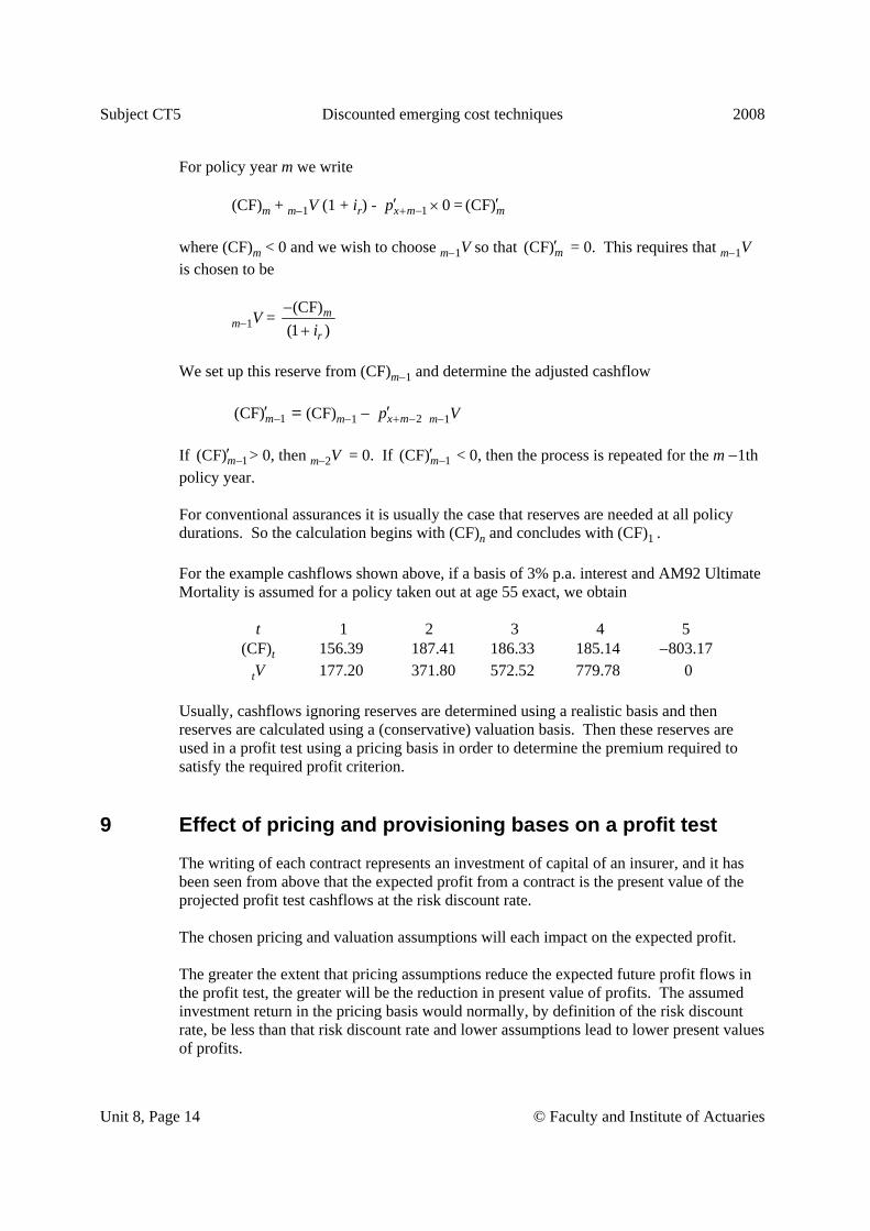
Subject CT5 Discounted emerging cost techniques 2008
Unit 8, Page 14 © Faculty and Institute of Actuaries
For policy year m we write (CF)m + m−1V (1 + ir) - 1 0x mp + −′ × = (CF)m′ where (CF)m < 0 and we wish to choose m−1V so that (CF)m′ = 0. This requires that m−1V is chosen to be
m−1V = (CF)(1 )
m
ri−+
We set up this reserve from (CF)m−1 and determine the adjusted cashflow 1(CF)m−′ = (CF)m−1 − 2x mp + −′ m−1V
If 1(CF)m−′ > 0, then m−2V = 0. If 1(CF)m−′ < 0, then the process is repeated for the m −1th policy year. For conventional assurances it is usually the case that reserves are needed at all policy durations. So the calculation begins with (CF)n and concludes with (CF)1 . For the example cashflows shown above, if a basis of 3% p.a. interest and AM92 Ultimate Mortality is assumed for a policy taken out at age 55 exact, we obtain t 1 2 3 4 5 (CF)t 156.39 187.41 186.33 185.14 −803.17 tV 177.20 371.80 572.52 779.78 0 Usually, cashflows ignoring reserves are determined using a realistic basis and then reserves are calculated using a (conservative) valuation basis. Then these reserves are used in a profit test using a pricing basis in order to determine the premium required to satisfy the required profit criterion.
9 Effect of pricing and provisioning bases on a profit test
The writing of each contract represents an investment of capital of an insurer, and it has been seen from above that the expected profit from a contract is the present value of the projected profit test cashflows at the risk discount rate. The chosen pricing and valuation assumptions will each impact on the expected profit. The greater the extent that pricing assumptions reduce the expected future profit flows in the profit test, the greater will be the reduction in present value of profits. The assumed investment return in the pricing basis would normally, by definition of the risk discount rate, be less than that risk discount rate and lower assumptions lead to lower present values of profits.

2008 Discounted emerging cost techniques Subject CT5
© Faculty and Institute of Actuaries Unit 8, Page 15
A valuation basis which gives rise to positive reserves will normally reduce the present value of profits from a contract. This is because the reserves reduce otherwise positive cashflows and are then invested in a relatively safe form of assets whose rate of investment return, by definition of the risk discount rate, is expected to be less than the risk discount rate. Over the whole term of a contract, and assuming that experience turns out to be in line with the assumed pricing basis, stronger reserves will not reduce the overall aggregate size of the cashflows but they will delay the cashflows so that they emerge later than they would have done using a weaker valuation basis, hence reducing the present value of profits. In the above description of the profit test calculations we have assumed that reserves are set up at the end of policy years, and this is conventionally how profit tests are carried out. However, it is more prudent to assume that reserves are set up at the beginning of policy years (as soon as a premium is paid). In this case, making the usual assumption that reserves will earn less than the risk discount rate, the profit would be slightly smaller. In practice, insurance companies would tend to calculate cashflows monthly rather than annually, and therefore the convention of year-end reserves does not lead to a material overstatement of profit. This is an example of a more general approach which can be used to discount cashflows, given sufficient computing power. That is, to discount cashflows as soon as they arise, rather than first accumulating them to the end of policy years at an assumed rate of interest. As explained above, this approach would be more prudent in the case of reserve cashflows but is actually more prudent for any other negative cashflows, expenses for example.

Subject CT5 Discounted emerging cost techniques 2008
Unit 8, Page 16 © Faculty and Institute of Actuaries
10 Multiple decrement service table for pensions calculations
Consider the following multiple state model.
Such a model can be used to represent the states and transitions for the members of a pension scheme. Contributions are paid while members are in the “active” state, benefits are paid when members move between states e.g. return of contributions on leaving, death in service benefit, or while members remain in a particular state e.g. age retirement and ill-health retirement pensions. To value contributions and benefits it is useful to be able to calculate the probabilities of transfer between particular states. For the active members of a scheme these transition probabilities can be presented in the form of a multiple decrement table. Such a table for the active members of a pension scheme is usually termed a service table.
Dead
d
Active
member
a
Alive and left the scheme
w
Retired at Normal Pension
Age (NPA)
r
Retired on ill health
grounds beforeNPA
i
*
*
*
*
2008 Discounted emerging cost techniques Subject CT5
© Faculty and Institute of Actuaries Unit 8, Page 17
The transition probabilities (sometimes called the dependent rates) are estimated using the methods described in Subject CT4, Models. They are displayed in a service table, which is constructed as follows: (i) For the lowest age at which there are active members of the scheme e.g. 20, 25;
choose a radix e.g. 20 for the service table, where 20 is a sufficiently large arbitrary integer number chosen so that any calculations completed using the service table will have the required accuracy.
(ii) Use the estimated and graduated transition probabilities ,1 ,1 ,1 ,1, , ,aw ar ai ad
x x x xp p p p x = 20, 21, 22 ... to calculate dx = ,1
adx xp
wx = ,1
awx xp
rx = ,1
arx xp
ix = ,1
aix xp
1x+ = x − dx − wx − rx − ix for x = 20, 21, 22, ... (iii) Display the service table as x x wx dx ix rx The valuations connected with a pension scheme will also need separate life tables for age retirement pensioners, ill-health retirement pensioners and deferred pensioners. In pension schemes where future benefits and contributions are directly related to future salary levels the valuation of such benefits and contributions will require the estimation of future salaries. This is achieved using a salary scale. Salaries are typically assumed to increase with age as a result of “merit” (promotional) increases and with time as a result of “inflationary” increases.

Subject CT5 Discounted emerging cost techniques 2008
Unit 8, Page 18 © Faculty and Institute of Actuaries
Using data about past merit increases (obtained by removing inflation from past salary trends) we can build up a salary scale unadjusted for inflation sx
* such that
**x t
x
ss
+ = salary expected to be received in age interval ( , 1) before inflationsalary expected to be received in age interval ( , 1) before inflation
x t x tx x
+ + ++
Inflationary increases can then be valued by adjusting for an assumed rate of inflation of f per annum, defining an inflation adjusted scale sx = (1 + f)x sx
*. This inflation adjusted salary scale is used throughout the remainder of this Unit. Care needs to be taken in using pension scheme service tables to understand what, if any, inflation adjustment has been applied to the salary scale. The table given in “Formulae and Tables for Examinations” contains both merit and inflation increases.
10.1 Updating a service table
10.1.1 Associated single decrement tables
For each of the causes in a multiple decrement or service table, it is possible to define a single decrement table which only involves a particular cause of decrement. In effect the other modes of decrement are assumed not to operate. We define functions as in any single decrement table except that each symbol has a superscript indicating the mode of decrement that is being modelled. Notation , , , ,j j j j j
x x x x xd q p μ etc. for mode of decrement j.
jxq is called an independent rate of decrement because its value is not influenced by other
decrements..
10.1.2 Relationships between single and multiple decrement tables
The linking assumption between the tables is ( ) j j
xxaμ = μ for all j and all x The assumption is often called the “independence of decrements”. One of its consequences is that if we observe the rates of decrement from cause j in two groups, one which includes all those who have not left the population as a result of decrement from cause i and the other which includes all those who have left the population as a result of decrement from cause i, then the observed rates of decrement from cause j in the two groups are the same. So the rate of decrement from cause j is independent of the rate from cause i.
2008 Discounted emerging cost techniques Subject CT5
© Faculty and Institute of Actuaries Unit 8, Page 19
There are a number of theoretical shortcomings of these assumptions but they are beyond the scope of this course and application of these assumptions provides us with a viable working model for actuaries in practice.
10.1.3 Obtaining the underlying single decrement tables from the multiple decrement table
We use the notation ( ) ( ),k kx xaq ad− − etc. for the decrement functions which exclude
decrement k. ( ) k
xaq − = ( ) ( )kx xaq aq− ( ) k
xad − = ( ) ( )kx xad ad− Assume that decrements from −k are uniformly distributed over (x, x+1) in the multiple decrement table. Then the ( ) k
xad − decrements will occur on average at age 12x + . Thus, if the causes −k
are eliminated, each one of these lives will be exposed to decrement from cause k for an average of 1
2 year in (x, x+1). The expected number of additional decrements from cause k in (x, x+1) will be: ( )1
2 .k kxxad q−
Thus, the total expected number of decrements in (x, x+1) if only cause k was operating is ( ) ( )1
2 .k k kxx xad ad q−+
This assumes non-selective decrements i.e. k after -k is same as k before -k. The number alive at the start of the interval is ( )xa . Therefore, the independent rate of decrement from cause k can be approximated by
12( ) ( ) .
( )
k k kx x xk
xx
ad ad qq
a
−+=
Giving { }1
2( ) ( ) ( )k k kx x x xa ad q ad−− =
i.e. 12
( )1 ( )
kk xx k
x
aqqaq −=
−
Subject CT5 Discounted emerging cost techniques 2008
Unit 8, Page 20 © Faculty and Institute of Actuaries
Thus, for two decrements α and β
xqα = ( ) ( )11 12 21
2
( ) ( ) 1 ( ) ( ) 1 ( )1 ( )
xx x x x
x
aq aq aq aq aqaq
α −α β α ββ = − ≈ +
−
and for 3 decrements α, β and γ:
( )1
2
( )=1 ( ) ( )
xx
x x
aqqaq aq
αα
β γ− +
≈ ( ){ }12( ) 1 ( ) ( )x x xaq aq aqα β γ+ +
These are amongst the most practical formulae. They enable the underlying single decrement tables to be obtained from an estimated multiple decrement table. The formulae depend upon the assumption of a uniform distribution of decrements α, β, γ etc. in the multiple decrement table.
10.1.4 Construction of multiple decrement tables from underlying single decrement tables
These results are often used when we need to adjust the observed ( )kxaq . That is making
observations fit for purpose for which they will be used, by updating the underlying rates for one or more of the causes of decrement so that they match the current experience. Sequence: ' '
modifyobserved used( ) ( )k k k k
x x x xaq q q aq⎯⎯→ ⎯⎯→ ⎯⎯→
The link relationship enables us to write
( )n xap = 0
exp ( )n
x ta dt+
⎧ ⎫⎪ ⎪− μ⎨ ⎬⎪ ⎪⎩ ⎭∫
= 0
exp ( ) ( ) ...n
x t x ta a dtα β+ +
⎧ ⎫⎪ ⎪− μ + μ⎨ ⎬⎪ ⎪⎩ ⎭∫
= 0 0
exp ( ) exp ( ) ...n n
x t x ta dt a dtα β+ +
⎧ ⎫ ⎧ ⎫⎪ ⎪ ⎪ ⎪− μ − μ⎨ ⎬ ⎨ ⎬⎪ ⎪ ⎪ ⎪⎩ ⎭ ⎩ ⎭∫ ∫
2008 Discounted emerging cost techniques Subject CT5
© Faculty and Institute of Actuaries Unit 8, Page 21
= 0 0
exp exp ...n n
x t x tdt dtα β+ +
⎧ ⎫ ⎧ ⎫⎪ ⎪ ⎪ ⎪− μ − μ⎨ ⎬ ⎨ ⎬⎪ ⎪ ⎪ ⎪⎩ ⎭ ⎩ ⎭∫ ∫
( )n xap = . ..........n x n xp pα β Rearrange the relationship to give (with n = 1) 1 ( ) (1 )(1 ) .....x x xaq q qα β− = − − ( )xaq = ........i i j i j k
x x x x x xi i j i j ki j i j k
q q q q q q≠ ≠ ≠
Σ − Σ Σ + Σ Σ Σ ............
Thus if we have , , ......x x xq q qα β γ etc., we can determine ( )xaq e.g. in a double (two) decrement table, with decrements α and β ( )xaq = .x x x xq q q qα β α β+ −
10.1.5 How to obtain multiple decrement table rates
( )xaq α = ( )( )
x
x
ada
α =
1
0
( ) ( ) .( )
tx t x t
xt
a a dta
= α+ +
=
μ∫
= 1
0
( ) . . .t
t xt x x t
t xt
pap dt
p
= αα+α
=
μ∫
using the assumption of the equal forces in the multiple and single decrement tables i.e. non-selective decrements. By using assumptions about the distribution of decrements in the single decrement table we can approximate the integrand and make it easy to evaluate. Suppose there are m decrements, and each one is uniformly distributed over each year of age in the single decrement table, then t x x tpα α
+μ = xqα i
t xp = 1 − it xq = 1 − t . i
xq i = β, γ, ... m
Subject CT5 Discounted emerging cost techniques 2008
Unit 8, Page 22 © Faculty and Institute of Actuaries
We know
( )t x
t x
appα
= ... mt x t x t xp p pβ γ
The integral simplifies to:
( )xaq α = 1
0
(1 . ) (1 . ) ... (1 . ) .t
mx x x x
t
q t q t q t q dt=
α β γ
=
− − −∫
= 1
2{1 ( ... )mx x x xq q q qα β γ− + + +
+ 1
3 ( ... )l mx x x xq q q qβ γ + +
− 1
4 ( .......................)x x xq q qβ γ δ ........................................} The result is cyclical. Here α is the decrement of interest and β, γ ... m are the competing decrements. The decrements are cycled to get the relationships needed. e.g double decrement table, decrements α and β ( )xaq α = (1 ½ )x xq qα β− ( )xaq β = (1 ½ )x xq qβ α− If we have estimated/know the single decrement rates, we can construct the multiple decrement table.
10.1.6 Alternative method of determining underlying single decrement rates
The subject of these equations can be changed to xqα and xqβ written in terms of ( ) ,xaq α so that the single decrement rates can be determined from the multiple decrement rates. They are of interest in life contingencies.
2008 Discounted emerging cost techniques Subject CT5
© Faculty and Institute of Actuaries Unit 8, Page 23
For example
xqα = ( )1 ½
x
x
aqq
α
β−
xqβ = ( )1 ½
x
x
aqq
β
α−
In this case of two decrements, quadratic equations are obtained which may be solved directly. With more than two decrements, iterative solutions are required to a set of simultaneous equations, setting initial estimates xqα = ( ) , = ( ) , ( ) ,x x x x xaq q aq q aqα β β γ γ= .
10.1.7 Consistency with the multiple state approach
Recall that, in Section 4.3 of Unit 7, we assumed two competing decrements and assumed that the transition intensities were constant between ages. If we make this alternative assumption then the integration in Section 10.1.5 above becomes
( )xaq α = 1
0( ) .t xap dtαμ∫
We leave it to the reader to show that the integral simplifies to give
( )xaq α = log( ) ( )log( )
xx
x
p aqap
α
which can be rearranged to give
xqα = ( )
( ) ( )1 (1 ( ) ( ) )x
x x
aqaq aq
x xaq aq
α
α β+α β− − − which in equation (4) in Unit 7 Section 4.3 we derived from the multiple state model in that Section.
11 Salary-related pensions benefits and contributions
11.1 Pension fund benefits for active members
11.1.1 Age retirement
Pension schemes usually have a fixed age e.g. 65, at which members normally retire on grounds of age. Sometimes this fixed age is termed normal pension age (NPA). In many schemes members can opt to retire at a range of ages before NPA e.g. 60 to 65. Such retirements are termed early retirements. The pension entitlement is usually related to the
Subject CT5 Discounted emerging cost techniques 2008
Unit 8, Page 24 © Faculty and Institute of Actuaries
length of pensionable service. Pensionable service is as defined in the scheme rules. Examples are the number of years of scheme membership at the date of retirement, the curtate number of years membership i.e. only complete years count. The pension entitlement for each year of pensionable service is usually related to the level of pensionable salary e.g. 1/80th of the salary at date of retirement for each year of service. The amount by which the pension increases for each year of service is termed the accrual rate. Pensionable salary is usually defined (in the scheme rules) in one of three ways: (i) annual rate of salary at retirement, termed final salary (ii) average annual salary in the last few years (usually 3 to 5 years) before retirement,
termed final average salary (iii) average annual salary during scheme membership, termed career-average salary or
lifetime earnings To mitigate the effects of inflationary increases salaries are sometimes revalued to the date of retirement using an index of prices or earnings before being averaged. In addition to, or in place of, part of pension entitlement some pension schemes provide a lump sum on retirement which is related to the pension entitlement (and thus to salary) e.g. 3 × amount of pension.
11.1.2 Ill-health retirement
Schemes usually allow members to retire on grounds of ill-health and receive a pension benefit after a minimum length of scheme service. To prevent selection against other scheme members, entitlement usually depends on evidence of ill-health being provided. Benefits are usually related to salary at the date of ill-health retirement in similar ways to age retirement benefits. However, pensionable service is usually more generous than under age retirement with years beyond those served in the scheme being credited to the member e.g. actual pensionable service subject to a minimum of 20 years, or pensionable service that would have been completed by normal retirement age.
11.1.3 Death in service benefit
The dependants of the active members of the scheme who die before NPA usually receive a lump sum at the date of the member’s death. This lump sum is usually a multiple of salary (rather than pensionable salary) at the date of death e.g. ×2 or ×4.
11.1.4 Scheme contributions
Members usually pay a fixed percentage of their salary each month i.e. effectively continuously during membership e.g. 5%, 0% (a non-contributory scheme). The employer pays a regular contribution equal to a percentage of the total salaries of members. This contribution is designed to meet the balance of the cost of the scheme. It may be varied

2008 Discounted emerging cost techniques Subject CT5
© Faculty and Institute of Actuaries Unit 8, Page 25
from time to time in order to satisfy this objective. The employer may also make special additional payments over a limited period to fund one-off shortfalls in a scheme.
11.2 Expected cashflows generated by pensions benefits and contributions
11.2.1 Classification of benefits
For the purposes of evaluating expected cashflows and determining the present value of liabilities arising from the cashflows it is useful to divide benefits into three types. An accrued benefit is a benefit that has been earned as a result of pensionable service (or credited service) prior to the valuation date e.g. a pension of n/80ths of final average salary where n is the number of years of past pensionable service at the valuation date. A future service benefit is a benefit that is expected to be earned as a result of pensionable service after the valuation date e.g. a pension of (65 − x)/80ths of final average salary on age retirement at NPA of 65 for a member aged x at the valuation date. Some benefits do not depend on either past or future service, although they may depend on total expected pensionable service. Such benefits are termed prospective service benefits e.g. a death in service benefit of 4 × salary at the date of death, a pension of m/80ths of final average salary at date of ill-health retirement where m is the total expected pensionable service before NPA. In determining expected cashflows and the present values of benefits (and contributions) it is usually most straightforward to determine the components that arise as a result of past service and future service separately, and then combine these to obtain the total expected cashflow or the total present value.
11.2.2 Expected cashflows for salary related benefits and contributions
Expected cashflows take the form of Expected Amount Payable × Probability of Payment
The expected amount payable is determined using the rules of the scheme and a salary scale appropriate to the scheme. The probabilities of payment are determined using a service table for the active members of the scheme, and life tables for each category of non-active member e.g. age retirements, ill-health retirements. The amounts for many benefits (and contributions) depend upon expected future salaries. These can be obtained using data about the amounts or rates of current salary and salary scale. We give some examples.
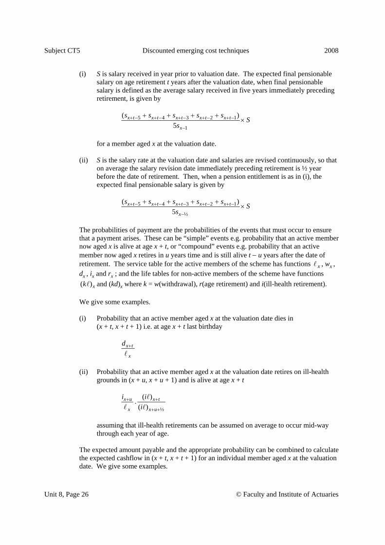
Subject CT5 Discounted emerging cost techniques 2008
Unit 8, Page 26 © Faculty and Institute of Actuaries
(i) S is salary received in year prior to valuation date. The expected final pensionable salary on age retirement t years after the valuation date, when final pensionable salary is defined as the average salary received in five years immediately preceding retirement, is given by
5 4 3 2 1
1
( )5
x t x t x t x t x t
x
s s s s s Ss
+ − + − + − + − + −
−
+ + + +×
for a member aged x at the valuation date. (ii) S is the salary rate at the valuation date and salaries are revised continuously, so that
on average the salary revision date immediately preceding retirement is ½ year before the date of retirement. Then, when a pension entitlement is as in (i), the expected final pensionable salary is given by
5 4 3 2 1
½
( )5
x t x t x t x t x t
x
s s s s s Ss
+ − + − + − + − + −
−
+ + + +×
The probabilities of payment are the probabilities of the events that must occur to ensure that a payment arises. These can be “simple” events e.g. probability that an active member now aged x is alive at age x + t, or “compound” events e.g. probability that an active member now aged x retires in u years time and is still alive t − u years after the date of retirement. The service table for the active members of the scheme has functions x , wx , dx , ix and rx ; and the life tables for non-active members of the scheme have functions ( )xk and (kd)x where k = w(withdrawal), r(age retirement) and i(ill-health retirement). We give some examples. (i) Probability that an active member aged x at the valuation date dies in
(x + t, x + t + 1) i.e. at age x + t last birthday
x t
x
d +
(ii) Probability that an active member aged x at the valuation date retires on ill-health
grounds in (x + u, x + u + 1) and is alive at age x + t
½
( ).( )
x u x t
x x u
i ii
+ +
+ +
assuming that ill-health retirements can be assumed on average to occur mid-way
through each year of age. The expected amount payable and the appropriate probability can be combined to calculate the expected cashflow in (x + t, x + t + 1) for an individual member aged x at the valuation date. We give some examples.
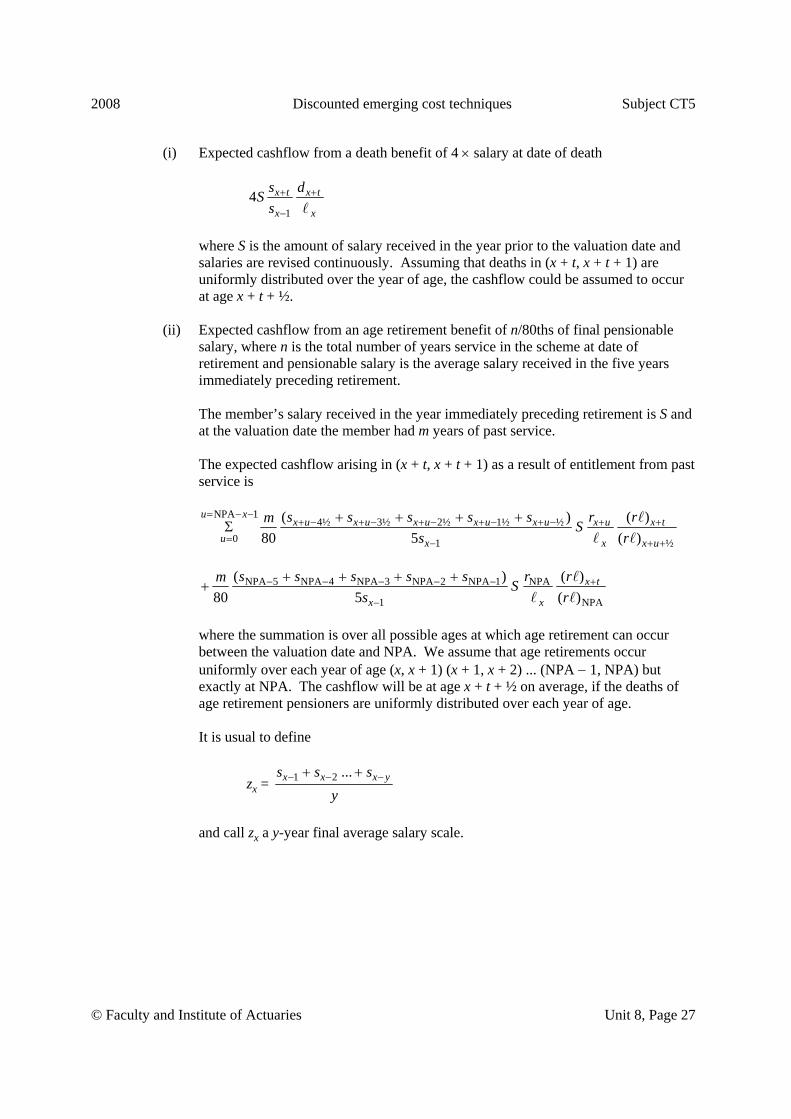
2008 Discounted emerging cost techniques Subject CT5
© Faculty and Institute of Actuaries Unit 8, Page 27
(i) Expected cashflow from a death benefit of 4 × salary at date of death
1
4 x t x t
x x
s dSs+ +
−
where S is the amount of salary received in the year prior to the valuation date and
salaries are revised continuously. Assuming that deaths in (x + t, x + t + 1) are uniformly distributed over the year of age, the cashflow could be assumed to occur at age x + t + ½.
(ii) Expected cashflow from an age retirement benefit of n/80ths of final pensionable
salary, where n is the total number of years service in the scheme at date of retirement and pensionable salary is the average salary received in the five years immediately preceding retirement.
The member’s salary received in the year immediately preceding retirement is S and
at the valuation date the member had m years of past service.
The expected cashflow arising in (x + t, x + t + 1) as a result of entitlement from past service is
NPA 14½ 3½ 2½ 1½ ½
0 1 ½
( ) ( )80 5 ( )
u xx u x u x u x u x u x u x t
u x x x u
s s s s s r rm Ss r
= − −+ − + − + − + − + − + +
= − + +
+ + + +Σ
NPA 5 NPA 4 NPA 3 NPA 2 NPA 1 NPA
1 NPA
( ) ( )80 5 ( )
x t
x x
s s s s s r rm Ss r
− − − − − +
−
+ + + ++
where the summation is over all possible ages at which age retirement can occur between the valuation date and NPA. We assume that age retirements occur uniformly over each year of age (x, x + 1) (x + 1, x + 2) ... (NPA − 1, NPA) but exactly at NPA. The cashflow will be at age x + t + ½ on average, if the deaths of age retirement pensioners are uniformly distributed over each year of age. It is usual to define
zx = 1 2 ...x x x ys s sy
− − −+ +
and call zx a y-year final average salary scale.
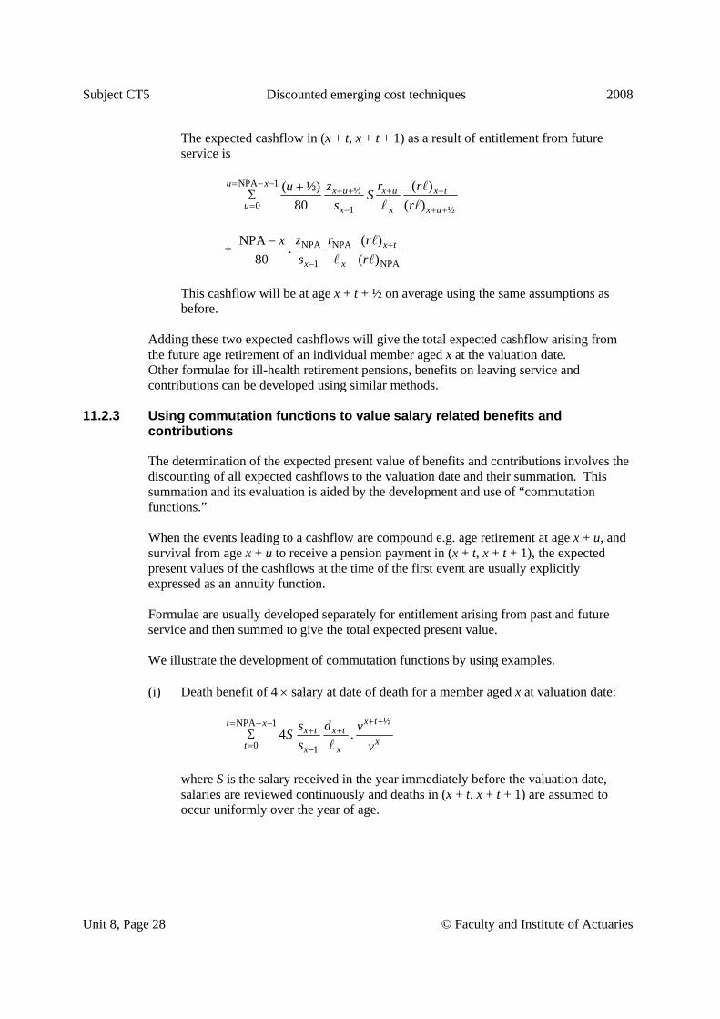
Subject CT5 Discounted emerging cost techniques 2008
Unit 8, Page 28 © Faculty and Institute of Actuaries
The expected cashflow in (x + t, x + t + 1) as a result of entitlement from future service is
NPA 1
½0 1 ½
( )( ½)80 ( )
u xx u x u x t
u x x x u
z r ru Ss r
= − −+ + + +
= − + +
+Σ
+ NPA NPA
1 NPA
( )NPA .80 ( )
x t
x x
z r rxs r
+
−
−
This cashflow will be at age x + t + ½ on average using the same assumptions as
before. Adding these two expected cashflows will give the total expected cashflow arising from the future age retirement of an individual member aged x at the valuation date. Other formulae for ill-health retirement pensions, benefits on leaving service and contributions can be developed using similar methods.
11.2.3 Using commutation functions to value salary related benefits and contributions
The determination of the expected present value of benefits and contributions involves the discounting of all expected cashflows to the valuation date and their summation. This summation and its evaluation is aided by the development and use of “commutation functions.” When the events leading to a cashflow are compound e.g. age retirement at age x + u, and survival from age x + u to receive a pension payment in (x + t, x + t + 1), the expected present values of the cashflows at the time of the first event are usually explicitly expressed as an annuity function. Formulae are usually developed separately for entitlement arising from past and future service and then summed to give the total expected present value. We illustrate the development of commutation functions by using examples. (i) Death benefit of 4 × salary at date of death for a member aged x at valuation date:
½NPA 1
0 14 .
x tt xx t x t
xt x x
s d vSs v
+ += − −+ +
= −Σ
where S is the salary received in the year immediately before the valuation date,
salaries are reviewed continuously and deaths in (x + t, x + t + 1) are assumed to occur uniformly over the year of age.
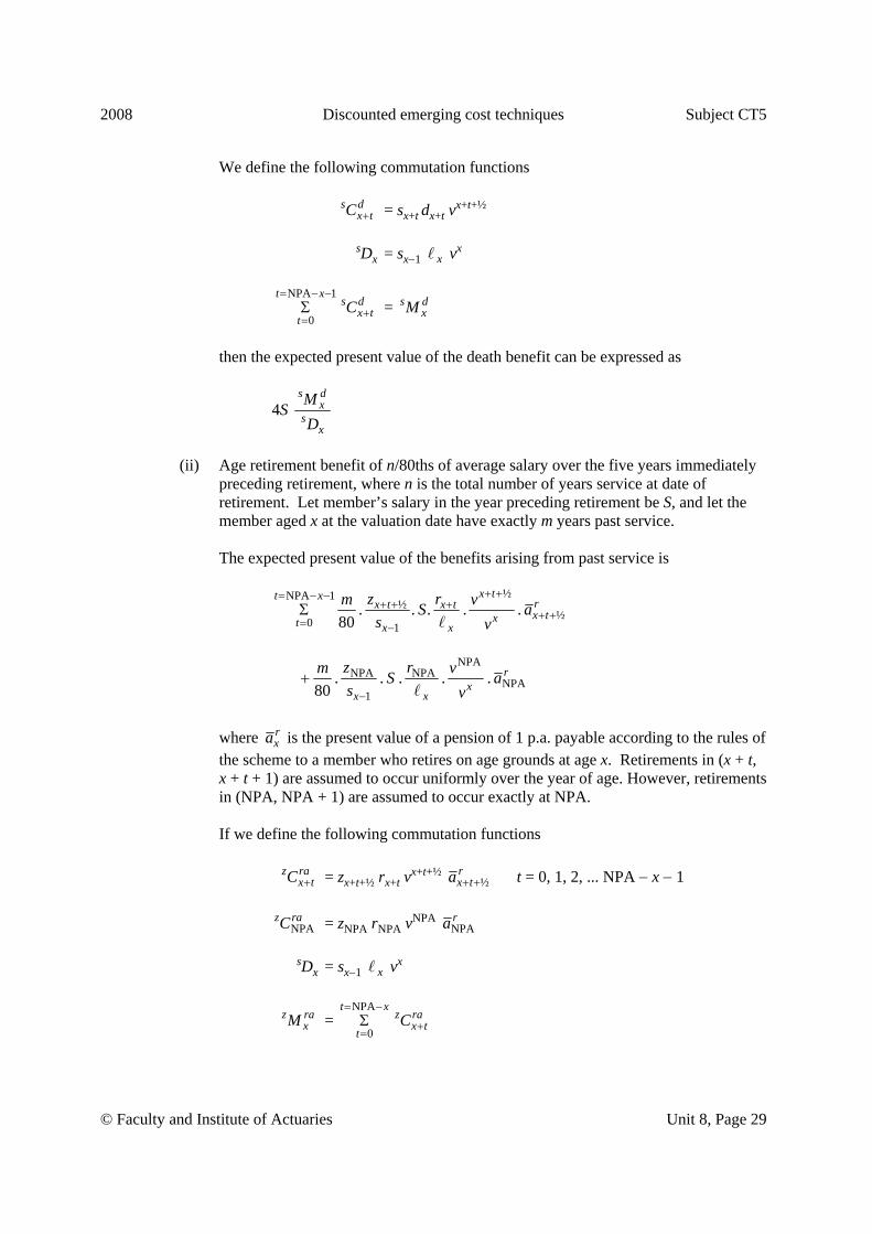
2008 Discounted emerging cost techniques Subject CT5
© Faculty and Institute of Actuaries Unit 8, Page 29
We define the following commutation functions s d
x tC + = sx+t dx+t vx+t+½
sDx = sx−1 x vx
NPA 1
0
t xs d
x ttC
= − −
+=Σ = s d
xM
then the expected present value of the death benefit can be expressed as
4S s d
xs
x
MD
(ii) Age retirement benefit of n/80ths of average salary over the five years immediately
preceding retirement, where n is the total number of years service at date of retirement. Let member’s salary in the year preceding retirement be S, and let the member aged x at the valuation date have exactly m years past service.
The expected present value of the benefits arising from past service is
½NPA 1
½½0 1
. . . . .80
x tt xrx t x tx txt x x
z rm vS as v
+ += − −+ + +
+ += −Σ
NPA
NPA NPANPA
1. . . . .
80r
xx x
z rm vS as v−
+
where r
xa is the present value of a pension of 1 p.a. payable according to the rules of the scheme to a member who retires on age grounds at age x. Retirements in (x + t, x + t + 1) are assumed to occur uniformly over the year of age. However, retirements in (NPA, NPA + 1) are assumed to occur exactly at NPA.
If we define the following commutation functions z ra
x tC + = zx+t+½ rx+t vx+t+½ ½
rx ta + + t = 0, 1, 2, ... NPA − x − 1
NPA
z raC = zNPA rNPA vNPA NPAra
sDx = sx−1 x vx
z raxM =
NPA
0
t xz ra
x ttC
= −
+=Σ

Subject CT5 Discounted emerging cost techniques 2008
Unit 8, Page 30 © Faculty and Institute of Actuaries
then the expected present value of the age retirement benefit as a result of past service can be written
80
z rax
sx
Mm SD
The expected present value at the valuation date (age x) of benefits arising from
future service in the year of age (x + t, x + t + 1) is
½
½½
1
1 1. . .2 80
x trx t x tx tx
x x
z r vS as v
+ ++ + +
+ +−
1½
1½ 11½
1
180
x trx t x tx tx
x x
z r vS as v
+ ++ + + +
+ +−
+
NPA 1 ½
NPA 1 ½ NPA 1NPA 1 ½
1
180
rx
x x
z r vS as v
− +− + −
− +−
+
NPA
NPA NPANPA
1
180
rx
x x
z r vS as v−
+
We define the following additional commutation function
z raxM =
NPA
0
12
t xz ra z ra
x t xtC C
= −
+=Σ −
and the expected present value can be written as
180
z rax t
sx
MSD
+
Now we add over all possible years of future service i.e. (x, x + 1) (x + 1, x + 2) ... (NPA − 1, NPA) to give the total expected present value of the age retirement
entitlement arising from all future service
NPA 1
0
180
z rat xx t
st x
MSD
= − −+
=Σ
If we define a commutation function
NPA 1
0
t xz ra
x ttM
= − −
+=Σ = z ra
xR

2008 Discounted emerging cost techniques Subject CT5
© Faculty and Institute of Actuaries Unit 8, Page 31
then the future liability can be expressed as
180
z rax
sx
RSD
and the total expected present value is
{ }180
z ra z rax xs
x
S m M RD
+
(iii) Members’ contributions are k% of salary assumed to be paid continuously i.e. on
average at mid-year. The expected present value of future contributions can be expressed as
½NPA 1
½0 1100
x tt xx t x t
xt x x
sk vSs v
+ += − −+ + +
= −Σ
We define the following commutation functions sDx = sx−1 vx x s
xD = sx vx+½ ½x+
sxN =
NPA 1
0
t xs
x ttD
= − −
+=Σ
and the total expected present value can be written as
100
sx
sx
Nk SD
The expected present values of the pensions benefits on ill-health retirement and the
benefits on leaving service can be evaluated using similar methods.
11.2.4 Terminology
Unlike the mainstream annuity and assurance terminology (usefully summarised for the interested reader in the “International Actuarial Notation” section of the “Formulae and Tables for Examinations” it is important to note that the commutation functions used above, to value pensions benefits and contributions, have no universally accepted definitions. Therefore, in any particular case, care needs to be taken to define carefully all symbols used. Similarly, the use of tables — such as that reproduced in the “Formulae and Tables
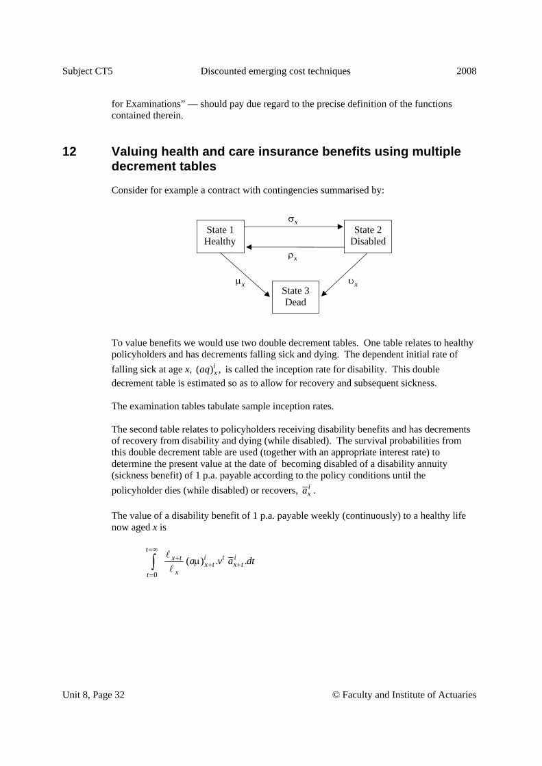
Subject CT5 Discounted emerging cost techniques 2008
Unit 8, Page 32 © Faculty and Institute of Actuaries
for Examinations” — should pay due regard to the precise definition of the functions contained therein.
12 Valuing health and care insurance benefits using multiple decrement tables
Consider for example a contract with contingencies summarised by:
To value benefits we would use two double decrement tables. One table relates to healthy policyholders and has decrements falling sick and dying. The dependent initial rate of falling sick at age x, ( ) ,i
xaq is called the inception rate for disability. This double decrement table is estimated so as to allow for recovery and subsequent sickness. The examination tables tabulate sample inception rates. The second table relates to policyholders receiving disability benefits and has decrements of recovery from disability and dying (while disabled). The survival probabilities from this double decrement table are used (together with an appropriate interest rate) to determine the present value at the date of becoming disabled of a disability annuity (sickness benefit) of 1 p.a. payable according to the policy conditions until the policyholder dies (while disabled) or recovers, i
xa . The value of a disability benefit of 1 p.a. payable weekly (continuously) to a healthy life now aged x is
0
( ) . .t
i t ix tx t x t
xt
a v a dt=∞
++ +
=
μ∫
State 2 Disabled
State 1 Healthy
State 3 Dead
σx
ρx
μx υx
2008 Discounted emerging cost techniques Subject CT5
© Faculty and Institute of Actuaries Unit 8, Page 33
The usual method of calculating the value of such benefits is to assume that lives becoming disabled in (x + t, x + t + 1) do so on average at age x + t + ½ (for all integral x) and to approximate this integral using
½
½
0
t i x t ix t x t
xxt
d v av
=∞ + ++ + +
=∑
This expression can be evaluated by defining and using commutation functions as follows
½½
0
ia i x ix x x
xx x
tia iax x t
t
C d v a
D v
M C
++
=∞
+=
=
=
=∑
so the value is approximated by
iax
x
MD
The “Formulae and Tables for Examinations” tabulate sample values for disability benefits.
13 Alternatives to the multiple decrement method
The main practical alternative to the multiple decrement approach is the multiple state approach described in Unit 7.
14 Non-life contingencies
The above techniques are flexible enough to value non-life contingencies. For example, an extended warranty insurance on a machine could be valued by assuming the policyholder is subject to three decrements: • withdrawal from the contract • failure of the machine (causing cessation of premiums and a claim payment) • death

Subject CT5 Discounted emerging cost techniques 2008
Unit 8, Page 34 © Faculty and Institute of Actuaries
Similarly, a charity could model a fixed term donation stream by assuming decrements of:: • non renewal of annual donation • death • end date of annual donation scheme being reached.
E N D

2008 Factors affecting mortality, selection and standardisation Subject CT5
© Faculty and Institute of Actuaries Unit 9, Page 1
UNIT 9 — FACTORS AFFECTING MORTALITY, SELECTION AND STANDARDISATION Syllabus objective (ix) Describe the principal forms of heterogeneity within a population and the ways in
which selection can occur. 1. State the principal factors which contribute to the variation in mortality and
morbidity by region and according to the social and economic environment, specifically:
• occupation • nutrition • housing • climate/geography • education • genetics
2. Define and give examples of the main forms of selection:
• temporary initial selection • class selection • time selection • spurious selection • adverse selection
3. Explain how selection can be expected to occur amongst individuals taking out
each of the main types of life insurance contracts, or amongst members of large pension schemes.
4. Explain why it is necessary to have different mortality tables for different
classes of lives. 5. Explain how decrements can have a selective effect. 6. Explain the theoretical basis of the use of risk classification in life insurance. 7. Explain the impact of the availability of genetic information on risk
classification in life insurance. 8. Explain the concept of a single figure index and its advantages and
disadvantages for summarising and comparing actual experience. 9. Define the terms crude mortality rate, directly standardised and indirectly
standardised mortality rate, standardised mortality ratio, and illustrate their use.

Subject CT5 Factors affecting mortality, selection and standardisation 2008
Unit 9, Page 2 © Faculty and Institute of Actuaries
1 Principal factors contributing to variation in mortality and morbidity
In addition to variation by age and sex, mortality and morbidity rates are observed to vary: • between geographical areas e.g. countries, regions of a country, urban and rural areas • by social class e.g. manual and non-manual workers • over time e.g. mortality rates usually decrease over time None of these categories e.g. geographical location and time, provide a direct (causal) explanation of the observed differences. Rather they are proxies for the real factors which cause the observed differences. Such factors are: • occupation • nutrition • housing • climate • education • genetics It is rare that observed differences in mortality can all be ascribed to a single factor. It is difficult to disentangle the effects of different factors as a result of confounding e.g. mortality rates of those living in sub-standard housing are (usually) higher than those of people living in good quality housing. However, those living in sub-standard housing usually have less well paid occupations and lower educational attainment than those living in good quality housing. Part or all of the observed difference may be due to these other differences and not to housing differences.
1.1 Occupation
Occupation can have several direct and indirect effects on mortality and morbidity. Occupation determines a person’s environment for 40 or more hours each week. The environment may be rural or urban, the occupation may involve exposure to harmful substances e.g. chemicals, or to potentially dangerous situations e.g. working at heights. Much of this is moderated by health and safety at work regulations. Some occupations are more healthy by their very nature e.g. bus drivers have a sedentary and stressful occupation while bus conductors are more active and less stressed. Some work environments e.g. publicans, give exposure to a less healthy lifestyle. Some occupations by their very nature attract more healthy or unhealthy workers. This may be accentuated by health checks made on appointment or by the need to pass regular health checks e.g. airline pilots. However, this effect can be produced without formal checks, e.g. former miners who have left the mining industry as a result of ill-health and then chosen to sell newspapers. This will inflate the mortality rates of newspaper sellers.

2008 Factors affecting mortality, selection and standardisation Subject CT5
© Faculty and Institute of Actuaries Unit 9, Page 3
A person’s occupation largely determines their income, and this permits them to adopt a particular lifestyle e.g. content and pattern of diet, quality of housing. This effect can be positive and negative e.g. over indulgence.
1.2 Nutrition
Nutrition has an important influence on morbidity and in the longer term on mortality. Poor quality nutrition can increase the risk of contracting many diseases and hinder recovery from sickness. In the longer term the burden of increased sickness can influence mortality. Excessive or inappropriate (e.g. too much fat) eating can lead to obesity and an increased risk of associated diseases (e.g. heart disease, hypertension) leading to increased morbidity and mortality. Inappropriate nutrition may be the result of economic factors e.g. lack of income to buy appropriate foods or the result of a lack of health and personal education resulting in poor nutritional choices. Also, social and cultural factors which encourage or discourage the eating of certain foods e.g. alcohol consumption.
1.3 Housing
The standard of housing encompasses not only all aspects of the physical quality of housing (e.g. state of repair, type of construction, heating, sanitation) but also the way in which the housing is used e.g. overcrowding and shared cooking. These factors have an important influence on morbidity, particularly that related to infectious diseases (e.g. from tuberculosis and cholera to colds and coughs) and thus on mortality in the longer term. The effect of poor housing is often confounded with the general effects of poverty.
1.4 Climate
Climate and geographical location are closely linked. Levels and patterns of rainfall and temperature lead to an environment which is amicable to certain kinds of diseases e.g. those associated with tropical regions. Effects can also be observed within these broad categories e.g. the differences between rural and urban areas in a geographical region. Some effects may be accentuated or mitigated depending upon the development of an area e.g. industry leading to better roads and communications. Natural disasters (such as tidal waves and famines) will also affect mortality and morbidity rates, and may be correlated to particular climates and geographical locations.
Subject CT5 Factors affecting mortality, selection and standardisation 2008
Unit 9, Page 4 © Faculty and Institute of Actuaries
1.5 Education
Education influences the awareness of the components of a healthy lifestyle which reduces morbidity and lowers mortality rates. It encompasses both formal education and more general awareness resulting from public health and associated campaigns. This effect manifests itself through many proximate determinants. • increased income • choice of a better diet • the taking of exercise • personal health care • moderation in alcohol consumption, smoking • awareness of dangers of drug abuse • awareness of a safe sexual lifestyle Some of these are direct causes of increased morbidity e.g. smoking and excessive alcohol consumption, leading to diseases such as lung and other forms of cancer, and strokes. A healthy lifestyle with improved fitness can lead to an enhanced ability to resist diseases.
1.6 Genetics
Genetics may give information about the likelihood of a person contracting particular diseases, and therefore may provide improved information about the chances of sickness or death. Such information may be used in isolation for the particular life in question or, more usefully, by combining it with the life histories of the current and past generations of the family. However, genetics is a relatively new area of study for the medical profession and only in the case of a few specific diseases is there as yet any indication that genetic information provides firm predictive evidence as to the chances of sickness or death relative to a person of average health. See also Section 7 below.
2 Selection
Selection is the process by which lives are divided into separate groups so that the mortality (or morbidity) within each group is homogeneous. That is, the experience of all lives within a particular group can be satisfactorily modelled by the same stochastic model of mortality (or morbidity). Sometimes the process of division is one that is imposed on the lives, e.g. the division of proposals for life assurance into classes. Lives in different classes will be charged according to different premium scales which reflect the mortality differences between the classes. Sometimes the process of division is one chosen by the lives themselves, e.g. deciding whether or not to purchase an immediate annuity. Those who purchase an annuity usually experience lighter mortality than those who decide not to purchase an annuity. The difference in mortality levels between groups is called the size of the select effect. Commonly occurring kinds of selection are classified into categories.
2008 Factors affecting mortality, selection and standardisation Subject CT5
© Faculty and Institute of Actuaries Unit 9, Page 5
2.1 Temporary initial selection
Each group is defined by a specified event (the select event) happening to all the members of the group at a particular age, e.g. buying a life assurance policy at age x, retiring on ill-health grounds at age x. A select mortality table (representing the stochastic model of mortality) is estimated for each group (see Unit 2). The mortality patterns in each group are observed to differ only for the first s years after the select event. The length of select period is s years. The differences are temporary, producing the phenomenon called temporary initial selection (see Unit 2).
2.2 Class selection
Each group is specified by a category or class of a particular characteristic of the population, e.g. sex with categories of male and female, occupation with categories of manual and non-manual employment. The stochastic models (life tables) are different for each class. There are no common features to the models, they are different for all ages. This is termed class selection.
2.3 Time selection
Within a population mortality (or morbidity) varies with calendar time. This effect is usually observed at all ages. The usual pattern is for mortality rates to become lighter (improve) over time, although there can be exceptions, due, for example, to the increasing effect of AIDS in some countries. A separate model or table will be produced for different calendar periods e.g. English Life Table No 14 1980–82 and English Life Table No 15 1990–92. The difference between the tables is termed time selection.
2.4 Adverse selection
Adverse selection is characterised by the way in which the select groups are formed rather than by the characteristics of those groups. So any of the previous forms of selection may also exhibit adverse selection. Adverse selection usually involves an element of self selection, which acts to disrupt (act against) a controlled selection process which is being imposed on the lives. This adverse selection tends to reduce the effectiveness of the controlled selection. Underwriting is the process by which life insurance companies divide lives into homogeneous risk groups by using the values of certain factors (rating factors) recorded for each life. If prospective policyholders know that a company does not use a particular rating factor, e.g. smoking status, then lives who smoke will opt to buy a policy from this company rather than a company that uses smoking status as a rating factor. The outcome will be to lessen the effect of the controlled selection being used by the company as part of the underwriting process. The effect of self selection by smokers is adverse to the company’s selection process. It is an example of adverse selection.
Subject CT5 Factors affecting mortality, selection and standardisation 2008
Unit 9, Page 6 © Faculty and Institute of Actuaries
2.5 Spurious selection
When homogeneous groups are formed we usually tacitly infer that the factors used to define each group are the cause of the differences in mortality observed between the groups. However, there may be other differences in composition between the groups, and it is these differences rather than the differences in the factors used to form the groups that are the true causes of the observed mortality differences. Ascribing mortality differences to groups formed by factors which are not the true causes of these differences is termed spurious selection. For example, when the population of England and Wales is divided by region of residence, some striking mortality differences are observed. However, a large part of these differences can be explained by the different mix of occupations in each region. The class selection ascribed to regions is spurious and is in part the effect of compositional differences in occupation between the regions. In statistical terminology the occupational differences in mortality are confounded (mixed up) with the regional differences.
3 Selection in life assurance and pensions business
3.1 Life assurance
Selection can arise as a result of decisions by the insurance company (underwriting) or as a result of decisions made by the policyholder (self selection). The aim of underwriting is to form homogeneous risk classes on the basis of sufficient rating factors so that the possibility of adverse selection by prospective policyholders is very small. Subsequent decisions made by those who take out policies, e.g. a decision to lapse the policy, can act as selective decrements in respect of the mortality risk. The initial underwriting process is based on a proposal form and sometimes a medical questionnaire and a medical examination selects out lives in better health. This is a form of class selection. The differences between those underwritten at different ages will usually only depend on policy duration for a limited period of time. Within the class of assured lives there is temporary initial selection. Each individual rating factor, e.g. occupation and alcohol consumption, will produce mortality differences that are an example of class selection. When a restricted number of rating factors are used, e.g. endowment assurances with limited evidence of health, there is more opportunity for adverse selection by prospective policyholders. The mortality levels amongst the class of assured lives tend to change over calendar time. This is an example of time selection. This effect may be the result of general improvements in mortality over time, or a result of changing underwriting standards over

2008 Factors affecting mortality, selection and standardisation Subject CT5
© Faculty and Institute of Actuaries Unit 9, Page 7
time. If the prime cause is the latter effect, and the observed changes are ascribed to improvements over time, this is an example of spurious selection. Withdrawal often acts as a selective decrement in respect of mortality. Those withdrawing tend to have lighter mortality than those who keep their policies in force. This selective effect results in mortality rates which increase markedly with policy duration and resembles temporary initial selection. Because the cause is not the effect of initial selection, but the effect of selective withdrawal, this is an example of spurious selection. Homogeneous lapse rates often result from subdivision by the method of selling the policy. This is an example of class selection. Lapse rates tend to be higher at shorter policy durations. This is an example of temporary initial selection.
3.2 Pension funds
A pension fund includes several different classes of lives each of which is subject to causes of decrement either from the scheme or from another class. The most important classes are: (i) active members of the scheme, i.e. those not in receipt of any benefits and for whom
contributions are being paid (ii) pensioners who retired at the normal retirement age and are now receiving a pension (iii) pensioners who retired under the ill-health retirement rules of the scheme and are
now receiving a pension benefit (iv) deferred pensioners, i.e. those for whom no contributions are currently being paid
and who are entitled to a pension at some future date (v) pensioners who retired under the early (before normal pension age) retirement rules
of the scheme and are now receiving a pension benefit For those currently paying contributions the decrements of interest are death, withdrawal and retirement. For those receiving benefit or entitled to a deferred benefit the only decrement of interest is death. The mortality of those who retired early (but in good health) or at normal retirement age is likely to be lower than that of ill-health retirement pensioners. This is an example of class selection. The mortality of ill-health retirement pensioners is likely to depend on duration since retirement for a few years following the date of retirement, and subsequently only on age attained. This is an example of temporary initial selection. Underwriting at the date of joining a scheme tends to be very limited, e.g. actively at work, and so there tends to be only very slight temporary initial selection. Different sections of a large scheme, e.g. works and staff, may exhibit different levels of mortality. This is an example of class selection.

Subject CT5 Factors affecting mortality, selection and standardisation 2008
Unit 9, Page 8 © Faculty and Institute of Actuaries
Among the active members of the scheme ill-health retirement acts as a selective decrement, resulting in lighter mortality among the remaining active members. This is sometimes termed the “healthy worker” or the “active lives mortality” effect. Withdrawal from a scheme is associated with voluntary or compulsory termination of employment (changing jobs or redundancy). If voluntary resignation is the cause this tends to select these with lighter mortality (and ill-health retirement) rates. If redundancy is the cause withdrawal rates tend to vary markedly over time as economic conditions vary. This is an example of time selection.
4 Why it is necessary to have different mortality tables for different classes of lives
When a life table is constructed it is assumed to reflect the mortality experience of a homogeneous group of lives i.e. all the lives to whom the table applies follow the same stochastic model of mortality represented by the rates in the table. This means that the table can be used to model the mortality experience of a homogeneous group of lives which is suspected to have a similar experience. If a life table is constructed for a heterogeneous group then the mortality experience will depend on the exact mixture of lives with different experiences that has been used to construct the table. Such a table could only be used to model mortality in a group with the same mixture. It would have very restricted uses. For this reason separate mortality tables are usually constructed for groups which are expected to be heterogeneous. This can manifest itself as class selection e.g. separate tables for males and females, whole life and term assurance policyholders, annuitants and pensioners, or as time selection e.g. separate tables for males in England and Wales in 1980–82 (ELT14) and 1990–92 (ELT15). Sometimes only parts of the mortality experience are heterogeneous e.g. the experience during the initial select period for life assurance policyholders, and the remainder are homogeneous e.g. the experience after the end of the select period for life assurance policyholders. In such cases the tables are separate (different) during the select period, but combined after the end of the select period. In fact there are separate (homogeneous) mortality tables for each age at selection, but they are tabulated in an efficient (space saving) way.

2008 Factors affecting mortality, selection and standardisation Subject CT5
© Faculty and Institute of Actuaries Unit 9, Page 9
5 How decrements can have a selective effect
One way in which lives in a population can be grouped is by the operation of a decrement (other than death) e.g. retiring on ill-health grounds, getting married, migrating to a new country. Those who do and do not experience this selective decrement will experience different levels of the primary decrement of interest, often mortality or morbidity. Those getting married usually experience lighter mortality and morbidity than those of the same age who do not get married. Marriage is said to have a selective effect in respect of mortality and morbidity.
6 Risk classification in life insurance
Life insurance companies provide a service of pooling independent homogeneous risks. If a company is able to do this then as a result of the Central Limit Theorem the profit per policy will be a random variable that follows the normal distribution with a known mean and standard deviation. The Central Limit Theorem was covered in Subject CT3, Probability and Mathematical Statistics. The company can use this result to set premium rates which ensure that the probability of a loss of a portfolio of policies is at an acceptable level. The independence of risks usually follows naturally from the way in which life insurance policies are sold. Rarely does the death of one policyholder influence the mortality of another policyholder. Careful underwriting is the mechanism by which the company ensures that its risk groups are homogeneous. The risk groups are defined by the use of rating factors, e.g. age, sex, medical history, height, weight, lifestyle. In theory, a company should continue to add rating factors to its underwriting system until the differences in mortality between the different categories of the next rating factor are indistinguishable from the random variation between lives that remains after using the current list of rating factors. In reality the ability of prospective policyholders to provide accurate responses to questions and the cost of collecting information also limit the extent to which rating factors can be used. For example, a proposal form should not ask for information which requires a specialist knowledge. Height is acceptable, but blood pressure is not. For example, the cost of undertaking extensive blood tests has to be weighed against the expected cost of claims that will be “saved” as a result of having this information. From a marketing point of view proposers are anxious that the process of underwriting should be straightforward and speedy. In practice, rating factors will be included if they avoid any possibility of selection against the company, and satisfy the time and cost constraints of marketing. This decision is often driven by competitive pressures. If several companies introduce a new rating factor, which in fact influences mortality levels significantly, then other companies will need to follow this lead or risk adverse selection against them.
Subject CT5 Factors affecting mortality, selection and standardisation 2008
Unit 9, Page 10 © Faculty and Institute of Actuaries
7 Impact of genetic information on risk classification in life insurance
To the extent that genetic information does actually provide useful predictive information — see Section 1.6 above — its use in risk classification then depends upon: • the extent to which genetic information is available to insurers. This is proving to be a
contentious legal and ethical issue, and drives at the heart of the equity argument about the extent to which risks should be pooled in an insurance mechanism as well as the associated public interest need to avoid the creation of a “genetic underclass.”
In the UK, the development of genetic testing has led to concerns that test information might be used by life insurance companies to set premiums. In fact, UK companies currently do not, and will not, ask individuals to take genetic tests as a condition of taking out insurance. The issue is whether, and under what circumstances, the results of a relevant genetic test that has already been taken should be given to an insurer. A five year moratorium on the use of DNA genetic test results by insurers was agreed by the industry in October 2001. The agreement covers all but the largest life insurance policies, enabling consumers to obtain up to £500,000 of life insurance, and £300,000 of critical illness, income protection and long-term care insurance, without having to disclose any genetic test results.
• how material the amended risk is, on account of the genetic information. It is likely that genetic information would be used only to the extent that it produces a material effect on the premium rating of a life in question. An even-handed approach suggests that whilst some premiums may be increased because the life poses an extra risk, some premiums might be reduced where the genetic information predicts a lesser than average chance of suffering an early death from particular diseases.
8 Use of single figure indices to summarise and compare mortality levels
Within any homogeneous population mortality experience will be summarised by age specific mortality rates and sometimes by graduating and displaying these results in a life table. If we wish to summarise the overall level of mortality in the population we are faced with the problem of evaluating the set of age specific rates. This is most simply done by calculating a single figure index which is a true reflection of the general level of mortality in the population. Such indices can also be used to facilitate the comparison between the mortality levels in two or more different populations, or within the same population at different points of time. All summary measures are weighted averages of the age specific rates or some function of the age specific rates. Averaging estimates of age specific rates, all of which are subject to
2008 Factors affecting mortality, selection and standardisation Subject CT5
© Faculty and Institute of Actuaries Unit 9, Page 11
sampling error, will give summary measures with much reduced sampling error. This will result in more precise comparisons. The calculation of some indices requires extensive data. This may limit the situations in which they can be used. Some indices involve the use of weights which vary between populations. In making comparisons using such indices we must be aware that observed differences in the index may be the result of different weights rather than the result of differing age specific rates in the populations being compared. The main advantage of the use of single figure indices is their simplicity for summary and comparison compared to the use of a set of age specific rates. Some indices are particularly designed for comparison with the mortality in a standard population, e.g. mortality rates used for premium calculation. This makes their use particularly relevant in an actuarial context. The main disadvantage of the use of single figure indices is the loss of information as a result of summarising the set of age specific rates, and any distortions that may be introduced by the choice of weights for the averaging process.
9 Single figure indices
Rates will be presented in the context of mortality but they can be used for any other decremental rates, e.g. retirement, disability inception, lapse. The following notation will be used
,cx tE Central exposed to risk in population being studied between ages x and
x + t. mx,t Central rate of mortality either observed or from a life table in population
being studied for ages x to x + t.
,s c
x tE Central exposed to risk for a standard population between x and x + t.
,s
x tm Central rate of mortality either observed or from a life table in standard population for ages x to x + t.

Subject CT5 Factors affecting mortality, selection and standardisation 2008
Unit 9, Page 12 © Faculty and Institute of Actuaries
9.1 Crude mortality rate
This summary measure is defined as
, ,
,
actual deathstotal exposed to risk
cx t x t
xcx t
x
E m
E
∑=
∑
It is a weighted average of mx,t using ,
cx tE as weights. Its main advantage is that a
knowledge of ,cx tE and mx,t separately for each age x is not needed. Its main disadvantage
is that differences in age structure i.e. ,cx tE between populations will be confounded with
differences between mortality rates in using this index to make comparisons of mortality levels between populations.
9.2 Directly standardised mortality rate
This summary measure is defined as
, ,
,
s cx t x t
xs c
x tx
E m
E
∑
∑
It is a weighted average of mx,t using ,
s cx tE as weights. Its main advantage is that it only
reflects differences in mx,t and not differences in age structures between populations. Its main disadvantage is that it requires age specific mortality rates mx,t for its calculation.
9.3 Indirectly standardised mortality rate
Indirect standardisation is an approximation to direct standardisation, and removes the need for a knowledge of the age specific mortality rates, mx,t. These rates are often not available or, because of the small age specific exposed to risk in the population being studied, are estimated with large standard errors. The crude mortality rate for the population being studied is easily calculated (see Section 8.1). We attempt to find a factor F *, such that directly standardised = F * × crude mortality mortality rate rate

2008 Factors affecting mortality, selection and standardisation Subject CT5
© Faculty and Institute of Actuaries Unit 9, Page 13
Simple substitution shows that
, , , ,
, ,*
s c cx t x t x t x t
x xs c c
x t x tx x
E m E mF
E E
∑ ∑=
∑ ∑
If we approximate mx,t in this ratio by smx,t , then we obtain a similar factor
, , , ,
, ,
s c s c sx t x t x t x t
x xs c c
x t x tx x
E m E mF
E E
∑ ∑=
∑ ∑
F is called the area comparability factor (a term resulting from its initial use in making comparisons between the different regions of England and Wales). If this approximation to F* is used then we obtain an indirectly standardised mortality rate
, , , ,
, , ,
s c s c sx t x t x t x t
x xs c c
x t x t x tx x
E m E m
E E m
∑ ∑
∑ ∑
Crude mortality rate Expected deaths in population
for standard population Actual deaths in population=
The main advantages of the indirectly standardised rate are the ease of availability of the data to calculate it, and the fact that it is a good approximation to the directly standardised rate and so removes almost all of the effect of differing age structures between populations when any comparisons are made.
9.4 Standardised mortality ratio
If we compare the indirectly standardised mortality rate with the crude mortality rate in the standard population i.e. a ratio, then we obtain
, ,
, ,
Actual deaths in populationExpected deaths in population
cx t x t
xc sx t x t
x
E m
E m
∑=
∑
This is effectively an indirectly standardised rate expressed on a scale where values less than 1 indicate populations with mortality lighter than that in the standard population and values greater than 1 indicate populations with mortality heavier than that in the standard population.

Subject CT5 Factors affecting mortality, selection and standardisation 2008
Unit 9, Page 14 © Faculty and Institute of Actuaries
The ratio can be written in the form
,, ,
,
, ,
x tc sx t x t sx x t
c sx t x t
x
mE m
m
E m
∑
∑
which shows it to be the weighted average of the age specific mortality differentials between the standard population and the population being studied
i.e. ,
,
x ts
x t
m
m
weighted by the age specific numbers of deaths in the standard population i.e. , ,
c sx t x tE m
E N D

abcd
Subject CT5 Contingencies Core Technical Syllabus with Cross Referencing to Core Reading for the 2008 Examinations 1 June 2007 The Faculty of Actuaries and Institute of Actuaries

Subject CT5 — Contingencies Core Technical Syllabus
Page 2
Aim The aim of the Contingencies subject is to provide a grounding in the mathematical techniques which can be used to model and value cashflows dependent on death, survival, or other uncertain risks. Links to other subjects Subjects CT1 — Financial Mathematics, CT3 — Probability and Mathematical Statistics and CT4 — Models: introduce techniques that will be drawn upon and used in the development of this subject. Subject ST2 — Life Insurance Specialist Technical: uses the principles and techniques in this subject to help in the solution of life insurance problems. Objectives On completion of this subject the candidate will be able to: (i) Define simple assurance and annuity contracts, and develop formulae for the means and
variances of the present values of the payments under these contracts, assuming constant deterministic interest. (Unit 1)
1. Define the following terms:
• whole life assurance • term assurance • pure endowment • endowment assurance • critical illness assurance • whole life level annuity • temporary level annuity • premium • benefit
including assurance and annuity contracts where the benefits are deferred. 2. Define the following probabilities: n|mqx , n|qx and their select equivalents n|mq[x]+r ,
n|q[x]+r .

Subject CT5 — Contingencies Core Technical Syllabus
Page 3
3. Obtain expressions in the form of sums for the mean and variance of the present value of benefit payments under each contract above, in terms of the curtate random future lifetime, assuming that death benefits are payable at the end of the year of death and that annuities are paid annually in advance or in arrear, and, where appropriate, simplify these expressions into a form suitable for evaluation by table look-up or other means.
4. Obtain expressions in the form of integrals for the mean and variance of the present
value of benefit payments under each contract above, in terms of the random future lifetime, assuming that death benefits are payable at the moment of death and that annuities are paid continuously, and, where appropriate, simplify these expressions into a form suitable for evaluation by table look-up or other means.
5. Extend the techniques of 3. and 4. above to deal with the possibility that premiums are
payable more frequently than annually and that benefits may be payable annually or more frequently than annually.
6. Define the symbols Ax , :x nA , 1
:x nA , 1:x nA , ax , :x na , :x nm a⏐ , xa , :x na , :m x na and
their select and continuous equivalents. Extend the annuity factors to allow for the possibility that payments are more frequent than annual but less frequent than continuous.
7. Derive relations between annuities payable in advance and in arrear, and between
temporary, deferred and whole life annuities. 8. Derive the relations Ax = 1 − xda , :x nA = 1 − :x nda , and their select and continuous
equivalents. 9. Define the expected accumulation of the benefits in 1., and obtain expressions for them
corresponding to the expected present values in 3., 4., and 5. (note: expected values only).
(ii) Describe practical methods of evaluating expected values and variances of the simple
contracts defined in objective (i). (Unit 2) 1. Describe the life table functions lx and dx and their select equivalents l[x]+r and d[x]+r . 2. Express the following life table probabilities in terms of the functions in 1.: n px , nqx ,
n|m qx and their select equivalents n p[x]+r , nq[x]+r , n|mq[x]+r . 3. Express the expected values and variances in objective (i) 3. in terms of the functions in
1. and 2.
Subject CT5 — Contingencies Core Technical Syllabus
Page 4
4. Evaluate the expected values and variances in objective (i) 3. by table look-up, where appropriate, including the use of the relationships in objectives (i) 7. and 8.
5. Derive approximations for, and hence evaluate, the expected values and variances in
objective (i) 4. in terms of those in objective (i) 3. 6. Evaluate the expected accumulations in objective (i) 9. 7. Describe practical alternatives to the life table which can be used to obtain the
evaluations in 4., 5., and 6. (iii) Describe and calculate, using ultimate or select mortality, net premiums and net premium
reserves of simple insurance contracts. (Unit 3) 1. Define the net random future loss under an insurance contract, and state the principle of
equivalence. 2. Define and calculate net premiums for the insurance contract benefits in objective (i) 1.
Premiums and annuities may be payable annually, more frequently than annually, or continuously. Benefits may be payable at the end of the year of death, immediately on death, annually, more frequently than annually, or continuously.
3. State why an insurance company will set up reserves. 4. Describe prospective and retrospective reserves. 5. Define and evaluate prospective and retrospective net premium reserves in respect of
the contracts in objective (i) 1., with premiums as in (iii) 2. 6. Show that prospective and retrospective reserves are equal when calculated on the same
basis. 7. Derive recursive relationships between net premium reserves at annual intervals, for
contracts with death benefits paid at the end of the year of death, and annual premiums. 8. Derive Thiele’s differential equation, satisfied by net premium reserves for contracts
with death benefits paid at the moment of death, and premiums payable continuously. 9. Define and calculate, for a single policy or a portfolio of policies (as appropriate):
• death strain at risk • expected death strain • actual death strain • mortality profit

Subject CT5 — Contingencies Core Technical Syllabus
Page 5
(iv) Describe the calculation, using ultimate or select mortality, of net premiums and net premium reserves for increasing and decreasing benefits and annuities. (Unit 4)
1. Extend the techniques of (ii) to calculate the expected present value of an annuity,
premium, or benefit payable on death, which increases or decreases by a constant compound rate. Calculate net premiums and net premium reserves for contracts with premiums and benefits which vary as described.
2. Define the symbols (IA)x , ( )xIa , and (Ia)x and their select equivalents. 3. Calculate the expected present value of an annuity, premium or benefit payable on
death, which increases or decreases by a constant monetary amount. Calculate net premiums and net premium reserves for contracts with premiums and benefits which vary as described.
4. Define with profits contract. 5. List the types of bonus that may be given to with profits contracts. 6. Calculate net premiums and net premium reserves for with profits contracts. (v) Describe the calculation of gross premiums and reserves of assurance and annuity contracts. (Unit 5) 1. List the types of expenses incurred in writing a life insurance contract. 2. Describe the influence of inflation on the expenses listed in 1. 3. Define the gross future loss random variable for the benefits and annuities listed in (i) 1.
and (iv). 4. Calculate gross premiums using the future loss random variable and the equivalence
principle. Premiums and annuities may be payable annually, more frequently than annually, or continuously. Benefits may be payable at the end of the year of death, immediately on death, annually, more frequently than annually, or continuously.
5. Calculate gross premiums using simple criteria other than the equivalence principle. 6. Calculate gross premium prospective reserves using the future loss random variable. 7. Define and calculate the gross premium retrospective reserve. 8. State the conditions under which, in general, the prospective reserve is equal to the
retrospective reserve allowing for expenses.

Subject CT5 — Contingencies Core Technical Syllabus
Page 6
9. Prove that, under the appropriate conditions, the prospective reserve is equal to the retrospective reserve, with or without allowance for expenses, for all standard fixed benefit and increasing/decreasing benefit contracts.
10. Derive a recursive relation between successive annual reserves for an annual premium
contract, with allowance for expenses, for standard fixed benefit contracts. (vi) Define and use straightforward functions involving two lives. (Unit 6) 1. Extend the techniques of objectives (i)–(v) to deal with cashflows dependent upon the
death or survival of either or both of two lives. 2. Extend the techniques of 1. to deal with functions dependent upon a fixed term as well
as age. (vii) Describe methods which can be used to model cashflows contingent upon competing risks. (Unit 7) 1. Explain how the value of a cashflow, contingent upon more than one risk, may be
valued using a multiple-state Markov Model. 2. Derive dependent probabilities from given transition intensities, using the Kolmogorov
equations introduced in Objective (vii) of the Models Subject. 3. Derive transition intensities from given dependent probabilities. (viii) Describe the technique of discounted emerging costs, for use in pricing, reserving, and
assessing profitability. (Unit 8) 1. Define unit-linked contract. 2. Evaluate expected cashflows for whole life, endowment and term assurances, annuities,
and unit-linked contracts. 3. Profit test simple annual premium contracts of the types listed in 2. and determine the
profit vector, the profit signature, the net present value, and the profit margin. 4. Show how the profit test may be used to price a product. 5. Show how the profit test may be used to determine reserves. 6. Describe the construction and use of multiple decrement tables, including the
relationships with associated single decrement tables.

Subject CT5 — Contingencies Core Technical Syllabus
Page 7
7. Use multiple decrement tables to evaluate expected cashflows dependent upon more than one decrement, including:
• pension benefits • other salary related benefits • health and care insurance
8. Describe practical alternatives to the multiple decrement table which can be used to
obtain the evaluations in 7. 9. Extend the techniques of 3., 6., and 7. to evaluate expected cashflows contingent upon
risks other than human life. (ix) Describe the principal forms of heterogeneity within a population and the ways in which
selection can occur. (Unit 9) 1. State the principal factors which contribute to the variation in mortality and morbidity
by region and according to the social and economic environment, specifically:
• occupation • nutrition • housing • climate/geography • education • genetics
2. Define and give examples of the main forms of selection:
• temporary initial selection • class selection • time selection • spurious selection • adverse selection
3. Explain how selection can be expected to occur amongst individuals taking out each of
the main types of life insurance contracts, or amongst members of large pension schemes.
4. Explain why it is necessary to have different mortality tables for different classes of
lives. 5. Explain how decrements can have a selective effect. 6. Explain the theoretical basis of the use of risk classification in life insurance.

Subject CT5 — Contingencies Core Technical Syllabus
Page 8
7. Explain the impact of the availability of genetic information on risk classification in life insurance.
8. Explain the concept of a single figure index and its advantages and disadvantages for
summarising and comparing actual experience. 9. Define the terms crude mortality rate, directly standardised and indirectly standardised
mortality rate, standardised mortality ratio, and illustrate their use.
End of Syllabus