16.548 coding, information theory (and advanced...

1

16.548 Coding, Information Theory (and

Advanced Modulation)

Prof. Jay WeitzenBall 411

[email protected]

2

Notes Coverage

• Course Introduction• Definition of Information and Entropy• Review of Conditional Probability

3

Class Coverage

• Fundamentals of Information Theory (4 weeks)

• Block Coding (3 weeks)• Advanced Coding and modulation as a way

of achieving the Shannon Capacity bound: Convolutional coding, trellis modulation, and turbo modulation, space time coding (7 weeks)

4

Course Web Site

• http://faculty.uml.edu/jweitzen/16.548– Class notes, assignments, other materials on

web site– Please check at least twice per week– Lectures will be streamed, see course website

5

Prerequisites (What you need to know to thrive in this class)

• 16.363 or 16.584 (A Probability class)• Some Programming (C, VB, Matlab)• Digital Communication Theory

6

Grading Policy• 4 Mini-Projects (25% each project)

•Lempel ziv compressor

• Cyclic Redundancy Check

• Convolutional Coder/Decoder soft decision

• Trellis Modulator/Demodulator

7

Course Information and Text Books

• Coding and Information Theory by Wells, plus his notes from University of Idaho

• Digital Communication by Sklar, or ProakisBook

• Shannon’s original Paper (1948)• Other material on Web site

8

Claude Shannon Founds Science of Information theory in 1948

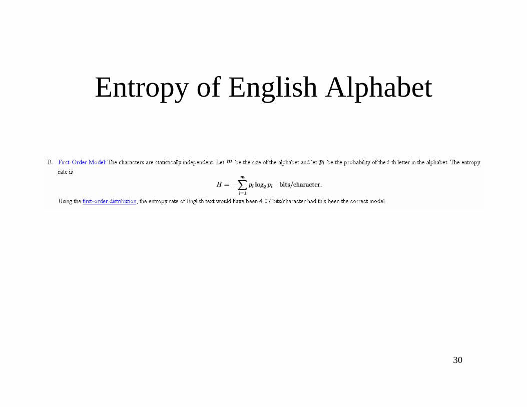
In his 1948 paper, ``A Mathematical Theory of Communication,'' Claude E. Shannon formulated the theory of data compression. Shannon established that there is a fundamental limit to lossless data compression. This limit, called the entropy rate, is denoted by H. The exact value of H depends on the information source --- more specifically, the statistical nature of the source. It is possible to compress the source, in a lossless manner, with compression rate close to H. It is mathematically impossible to do better than H.

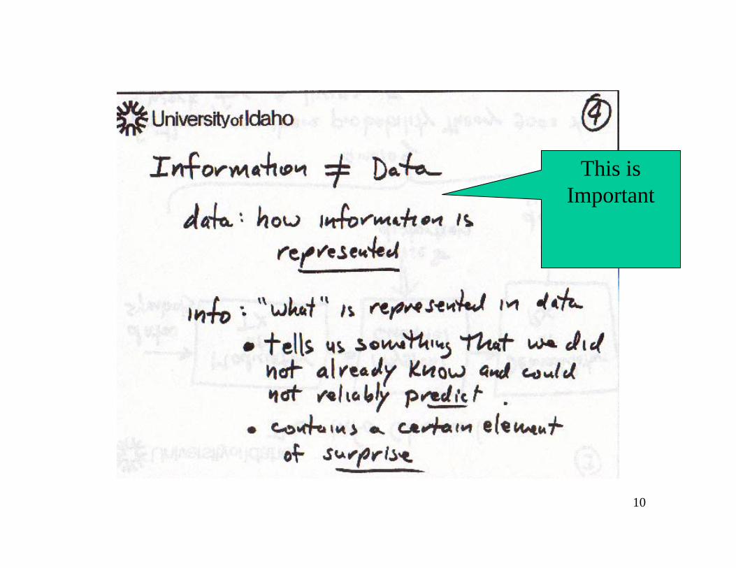
10

This is Important

11

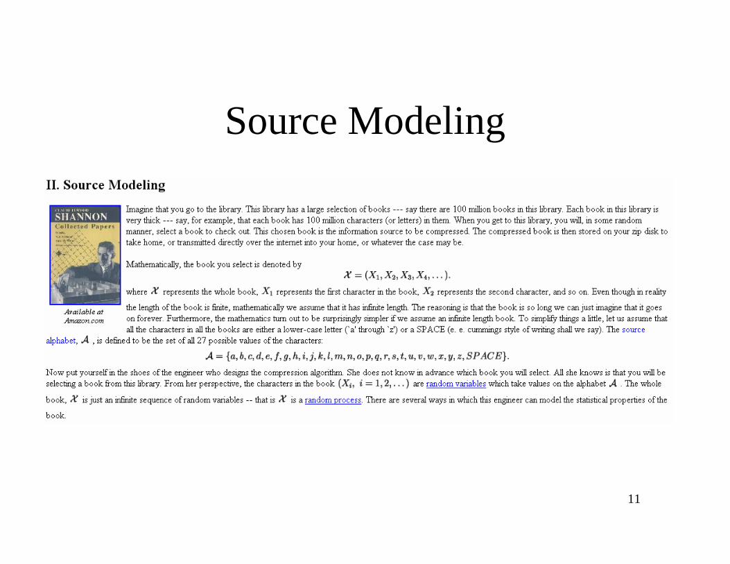
Source Modeling

12

Zero order models

It has been said, that if you get enough monkeys, and sit them down at enough typewriters, eventually they will complete the works of Shakespeare

13

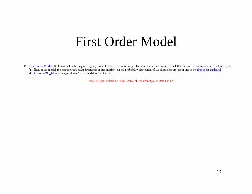
First Order Model

14

Higher Order Models

21

Zero’th Order Model

23

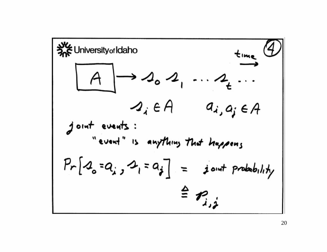
Definition of Entropy

Shannon used the ideas of randomness and entropy from the study of thermodynamics to estimate the randomness (e.g. information content or entropy) of a process

Entropy is a measure of predictability or randomness

24

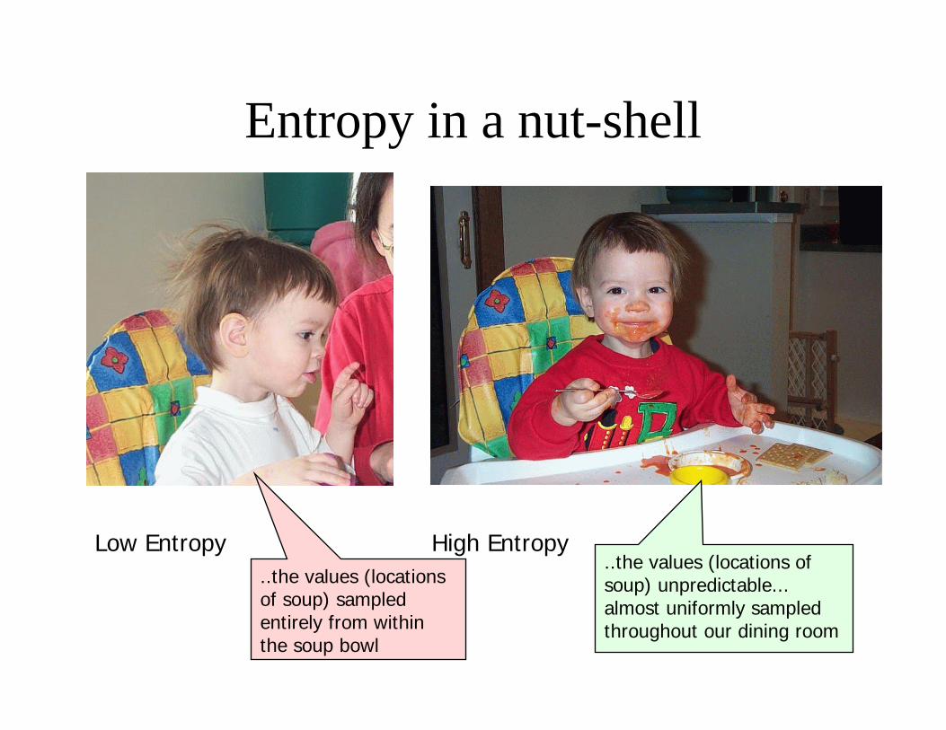
Entropy in a nut-shell

Low Entropy High Entropy..the values (locations of soup) unpredictable... almost uniformly sampled throughout our dining room

..the values (locations of soup) sampled entirely from within the soup bowl

25

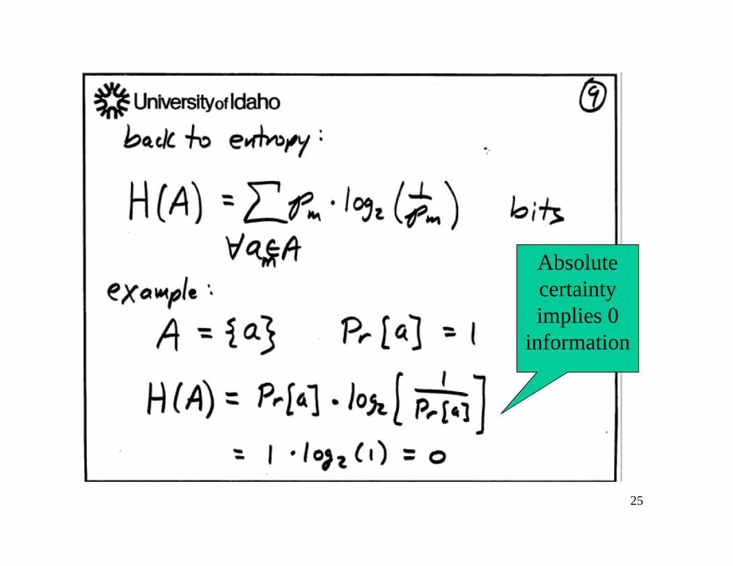
Absolute certainty implies 0

information

26

Randomness has high information

content

27

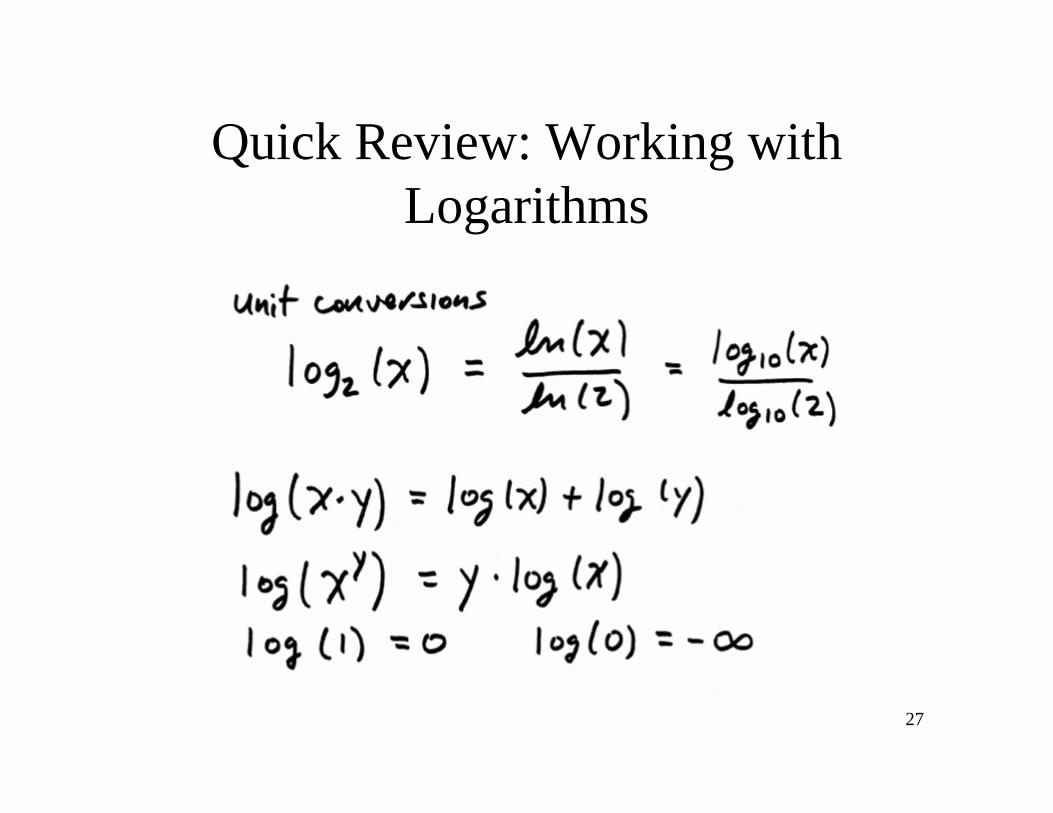
Quick Review: Working with Logarithms

30

Entropy of English Alphabet

36

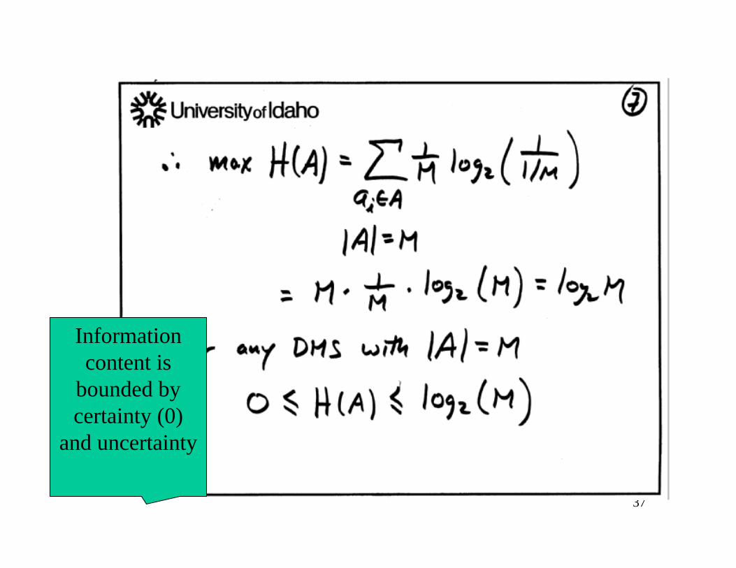
Kind of Intuitive,

but hard to prove

37

Information content is

bounded by certainty (0)

and uncertainty

39

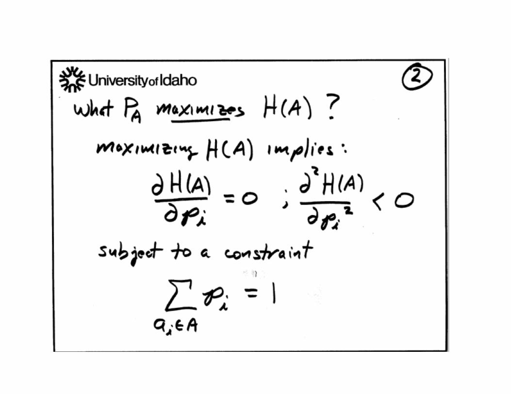
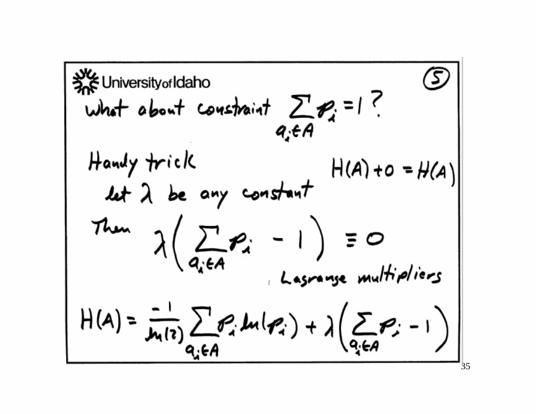
Bounds on Entropy

40

Math 495 Micro-Teaching

Quick Review:JOINT DENSITY OF

RANDOM VARIABLES

David ShermanBedrock, USA

41

In this presentation, we’ll discuss the joint density of two random variables. This is a mathematical tool for representing the interdependence of two events.

First, we need some random variables.

Lots of those in Bedrock.

42

Let X be the number of days Fred Flintstone is late to work in a given week. Then X is a random variable; here is its density function:

Amazingly, another resident of Bedrock is late with exactly the same distribution. It’s...

Fred’s boss, Mr. Slate!

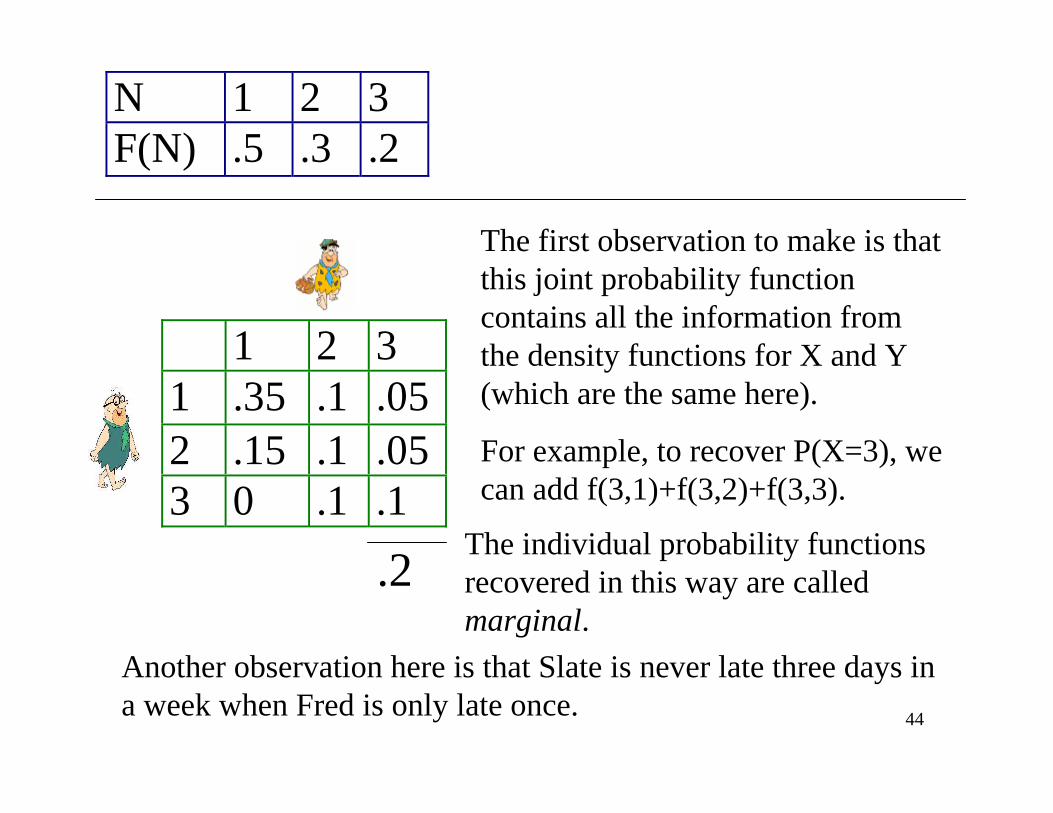
N 1 2 3F(N) .5 .3 .2

43

N 1 2 3F(N) .5 .3 .2

Remember this means that P(X=3) = .2.

Let Y be the number of days when Slate is late. Suppose we want to record BOTH X and Y for a given week. How likely are different pairs?

We’re talking about the joint density of X and Y, and we record this information as a function of two variables, like this:

1 2 31 .35 .1 .052 .15 .1 .053 0 .1 .1

This means that

P(X=3 and Y=2) = .05.

We label it f(3,2).

44

N 1 2 3F(N) .5 .3 .2

1 2 31 .35 .1 .052 .15 .1 .053 0 .1 .1

The first observation to make is that this joint probability function contains all the information from the density functions for X and Y (which are the same here).

For example, to recover P(X=3), we can add f(3,1)+f(3,2)+f(3,3).

.2The individual probability functions recovered in this way are called marginal.

Another observation here is that Slate is never late three days in a week when Fred is only late once.

45

N 1 2 3F(N) .5 .3 .2

Since he rides to work with Fred (at least until the directing career works out), Barney Rubble is late to work with the same probability function too. What do you think the joint probability function for Fred and Barney looks like?

1 2 31 .5 0 02 0 .3 03 0 0 .2

It’s diagonal!

This should make sense, since in any week Fred and Barney are late the same number of days.

This is, in some sense, a maximum amount of interaction: if you know one, you know the other. P(Barneylate |Fred late)= 1

46

N 1 2 3F(N) .5 .3 .2A little-known fact: there is actually another famous person who is late to work like this. SPOCK!

Before you try to guess what the joint density function for Fredand Spock is, remember that Spock lives millions of miles (and years) from Fred, so we wouldn’t expect these variables to influence each other at all.

(Pretty embarrassing for a Vulcan.)

In fact, they’re independent….

47

N 1 2 3F(N) .5 .3 .2

1 2 31 .25 .15 .12 .15 .09 .063 .1 .06 .04

Since we know the variables X and Z (for Spock) are independent, we can calculate each of the joint probabilities by multiplying.

For example, f(2,3) = P(X=2 and Z=3)

= P(X=2)P(Z=3) = (.3)(.2) = .06.

This represents a minimal amount of interaction. P(spock|fred)=P(spock)

48

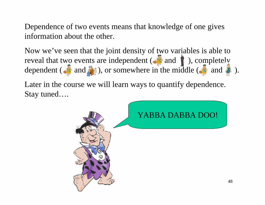
Dependence of two events means that knowledge of one gives information about the other.

Now we’ve seen that the joint density of two variables is able to reveal that two events are independent ( and ), completely dependent ( and ), or somewhere in the middle ( and ).

Later in the course we will learn ways to quantify dependence. Stay tuned….

YABBA DABBA DOO!

53

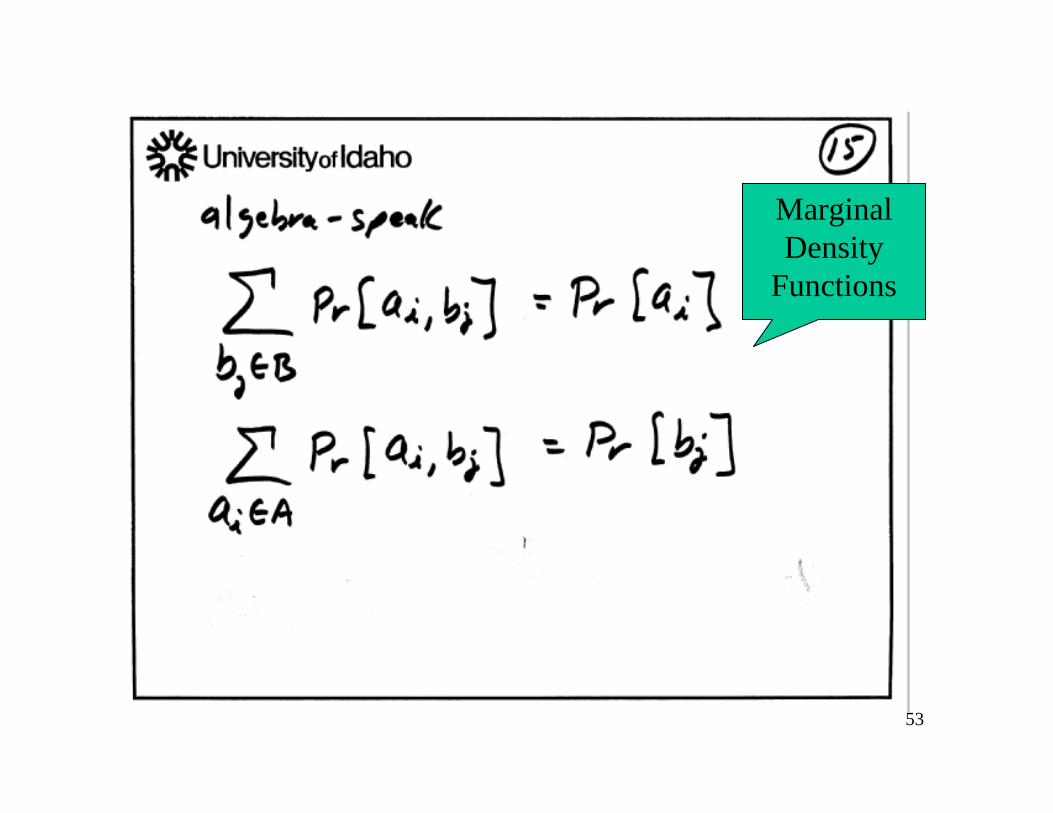
Marginal Density

Functions

54

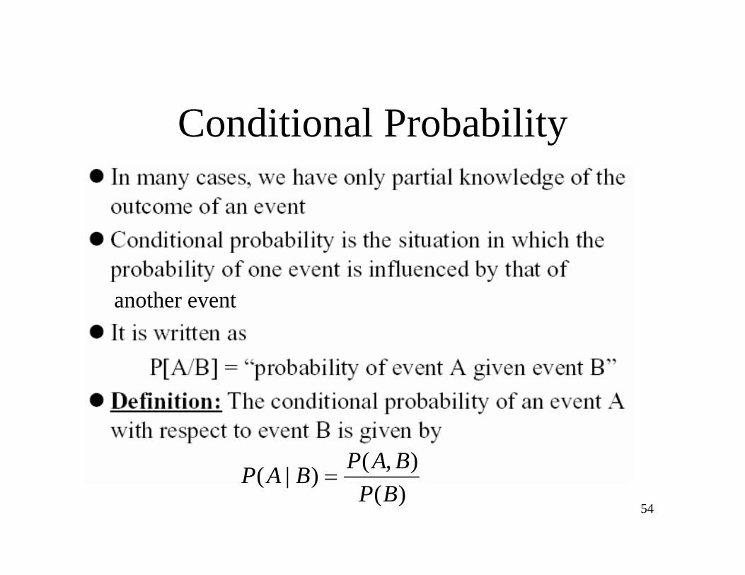
Conditional Probability

another event

)(),()|(

BPBAPBAP =

55

Conditional Probability (cont’d)

P(B|A)

56

Definition of conditional probability• If P(B) is not equal to zero, then the conditional probability of A

relative to B, namely, the probability of A given B, is

P(A|B) = P(A B)

P(B)∩

P(A B) = P(B) P(A|B)orP(A B) = P(A) P(B|A)

∩ •

∩ •

57

Conditional Probability

0.450.25 0.25

A B

P(A) = 0.25 + 0.25 = 0.50P(B) = 0.45 + 0.25 = 0.70P(A’) = 1 - 0.50 =0.50P(B’)= 1-0.70 =0.30

P(A|B) = P(A B)

P(B)∩

= =025070

0357..

.

P(B|A) = P(A B)

P(A)∩

= =025050

05..

.

58

Some Observations:

• In previous Slides P(Fred late and Spock late) were independent– Therefore P(Fred|Spock)

=P(Fred)P(spock)/P(spock)=P(Fred)• P(Fred late and Barney late) are totally

dependent– P(Fred|Barney)=1

59

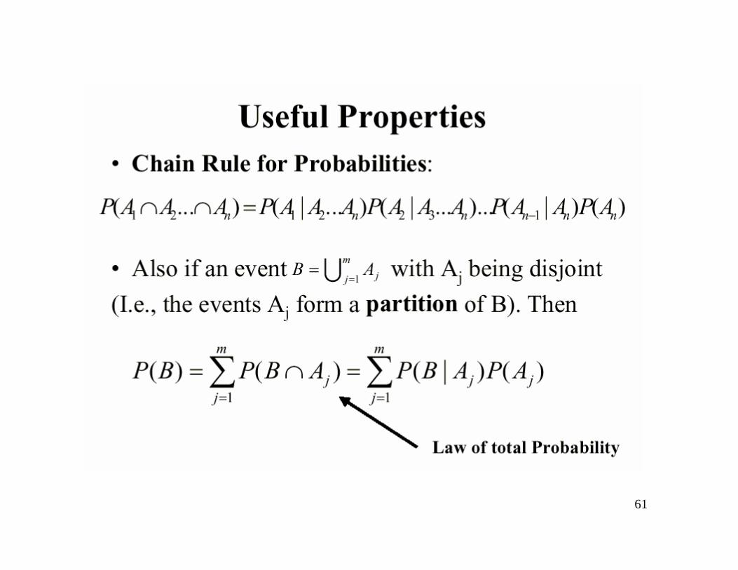
Law of Total Probability

If B B ,......, and B are mutually exclusive events of which one must occur, then for any event A

P(A) = P(B P(A|B + P(B

1 2 k

1 1 2

,

) ) ) ( | ) ...... ( ) ( | )⋅ ⋅ + + ⋅P A B P B P A Bk k2

P A P B P A B P B P A B( ) ( ) ( | ) ( ) ( | )' '= ⋅ + ⋅

Special case of rule of Total Probability

60

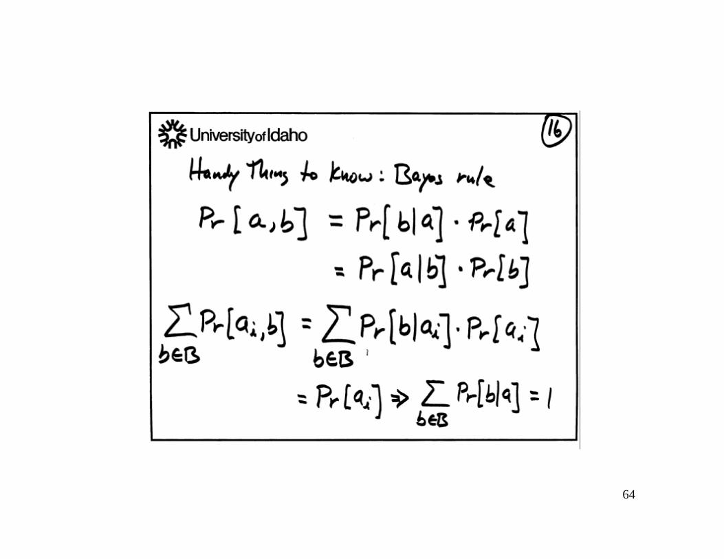
Bayes Theorem

62

Generalized Bayes’ theoremIf B B and B are mutually exclusive events of which one must occur, then

1 2 k, ,....

)/()(.......)/()()/()()/()()/(

2211 kk

iii BAPBPBAPBPBAPBP

BAPBPABP⋅++⋅+⋅

⋅=

k. 2,......, 1,=i for

63

Urn Problems

• Applications of Bayes Theorem• Begin to think about concepts of Maximum

likelihood and MAP detections, which we will use throughout codind theory

67

End of Notes 1

16.548 coding, information theory (and advanced...

Documents