168mm p1: tix/xyz p2: abc 16 - computer science...

P1: TIX/XYZ P2: ABCJWST201-c16 JWST201-Virtanen August 31, 2012 8:59 Printer Name: Yet to Come Trim: 244mm × 168mm

16Computational Auditory SceneAnalysis and Automatic SpeechRecognitionArun Narayanan, DeLiang WangThe Ohio State University, USA

16.1 Introduction

The human auditory system is, in a way, an engineering marvel. It is able to do wonderfulthings that powerful modern machines find extremely difficult. For instance, our auditorysystem is able to follow the lyrics of a song when the input is a mixture of speech andmusical accompaniments. Another example is a party situation. Usually there are multiplegroups of people talking, with laughter, ambient music and other sound sources running in thebackground. The input our auditory system receives through the ears is a mixture of all these.In spite of such a complex input, we are able to selectively listen to an individual speaker,attend to the music in the background, and so on. In fact this ability of ‘segregation’ is soinstinctive that we take it for granted without wondering about the complexity of the problemour auditory system solves.

Colin Cherry, in the 1950s, coined the term ‘cocktail party problem’ while trying to describehow our auditory system functions in such an environment [12]. He did a series of experimentsto study the factors that help humans perform this complex task [11]. A number of theories havebeen proposed since then to explain the observations made in those experiments [11,12,70].Helmhotz had, in the mid-nineteenth century, reflected upon the complexity of this signal byusing the example of a ball room setting [22]. He remarked that even though the signal is“complicated beyond conception,” our ears are able to “distinguish all the separate constituentparts of this confused whole.”

So how does our auditory system solve the so-called cocktail party problem? Bregman triedto give a systematic account in his seminal 1990 book Auditory Scene Analysis [8]. He calls

Techniques for Noise Robustness in Automatic Speech Recognition, First Edition.Edited by Tuomas Virtanen, Rita Singh, and Bhiksha Raj.© 2013 John Wiley & Sons, Ltd. Published 2013 by John Wiley & Sons, Ltd.

433


434 Techniques for Noise Robustness in Automatic Speech Recognition

the process “scene analysis” by drawing parallels with vision. It has been argued that the goalof perception is to form a mental description of the world around us. Our brain analyzes thescene and forms mental representations by combining the evidence that it gathers throughthe senses. The role of audition is no different. Its goal is to form a mental description of theacoustic world around us by integrating sound components that belong together (e.g., thoseof the target speaker in a party) and segregating those that do not. Bregman suggests that theauditory system accomplishes this task in two stages. First, the acoustic input is broken downinto local time-frequency elements, each belonging to a single source. This stage is calledsegmentation as it forms locally grouped time-frequency regions or segments [79]. The secondstage then groups the segments that belong to the same source to form an auditory stream. Astream corresponds to a single source.

Inspired by Bregman’s account of auditory organization, many computational systemshave been proposed to segregate sound mixtures automatically. Such algorithms have im-portant practical applications in hearing aids, automatic speech recognition, automatic musictranscription, etc. The field is collectively termed Computational Auditory Scene Analysis(CASA).

This chapter is about CASA and automatic speech recognition in noise. In Section 16.2, wediscuss some of the grouping principles of auditory scene analysis (ASA), focusing primarilyon the cues that are most important for the auditory organization of speech. We then move onto computational aspects. How to combine CASA and ASR effectively is, in itself, a researchissue. We address this by discussing CASA in depth, and introducing an important goal ofCASA - Ideal Binary Mask (IBM) - in Section 16.3. As we will see, the IBM has applicationsto both speech segregation and automatic speech recognition. We will also discuss a typicalarchitecture of CASA systems in Section 16.3. This will be followed by a discussion ofstrategies used for IBM estimation in Section 16.4. In the subsequent section, we address thetopic of robust automatic speech recognition, where we will discuss some of the methods tointegrate CASA and ASR. We note that this topic will also be addressed in other chapters(see Chapters 14 and 15 for detailed descriptions on missing-data ASR techniques). Finally,Section 16.6 offers a few concluding remarks.

16.2 Auditory Scene Analysis

CASA-based systems use ASA principles as a foundation to build computational models. Asmentioned in the introductory section, Bregman described ASA to be a two stage processwhich results in integration of acoustic components that belong together and segregation ofthose that do not. In the first stage, an acoustic signal is broken down into time-frequency (T-F)segments. The second stage groups segments formed in the first stage into streams. Groupingof segments can occur across frequency or across time. They are called simultaneous groupingand sequential grouping, respectively.

A number of factors influence the grouping stage which results in the formation of coherentstreams from local segments. Two distinctive schemes have been described by Bregman:primitive grouping and schema-based grouping.

Primitive grouping is an innate bottom-up process that groups segments based on acousticattributes of sound sources. Major primitive grouping principles include proximity, periodicity,continuity, common onset/offset, amplitude and frequency modulation, and spatial location [8,79]. Proximity refers to closeness in time or frequency of sound components. The components


Computational Auditory Scene Analysis and Automatic Speech Recognition 435

of a periodic signal are harmonically related (they are multiples of the fundamental frequencyor F 0), and thus segments that are harmonically related are grouped together. Periodicity is amajor grouping cue that has also been widely utilized by CASA systems. Continuity refers tothe continuity of pitch (perceived fundamental frequency), spectral and temporal continuity,etc. Continuity or smooth transitions can be used to group segments across time. Segmentsthat have synchronous onset or offset times are usually associated with the same sourceand hence, grouped together. Among the two, onset synchrony is a stronger grouping cue.Similarly, segments that share temporal modulation characteristics (amplitude or frequency)tend to be grouped together. If segments originate from the same spatial location, there is ahigh probability that they belong to the same source and hence should be grouped.

Unlike primitive grouping, schema-based grouping is a top-down process where groupingoccurs based on the learned patterns of sound sources. Schema-based organization plays animportant role in grouping segments of speech and music, as some of their properties arelearned over time by the auditory system. An example is the identification of a vowel based onobserved formants. Note that both schema-based and primitive grouping play important rolesin organizing real-world signals like speech and music.

The grouping principles introduced thus far were originally found though laboratory ex-periments using simple stimuli such as tones. Later experiments using more complex speechstimuli have established their role in speech perception [2,8]. Figure 16.1 shows some ofthe primitive grouping cues present for speech organization. Cues like continuity, commononset/offset, harmonicity are marked in the figure.

16.3 Computational Auditory Scene Analysis

Wang and Brown define CASA as ([79], p. 11):

. . . the field of computational study that aims to achieve human performance in ASA by using oneor two microphone recordings of the acoustic scene.

This definition takes into account the biological relevance of this field by limiting the numberof microphones to two (like in humans) and the functional goal of CASA. The mechanismsused by CASA systems are perceptually motivated. For example, most systems make use ofharmonicity as a grouping cue [79]. But this does not mean that the systems are exclusivelydependent on ASA to achieve their goals. As we will see, modern systems make use ofperceptual cues in combination with methods not necessarily motivated from the biologicalperspective.

16.3.1 Ideal Binary Mask

The goal of ASA is to form perceptual streams corresponding to the sound sources from theacoustic signal that reaches our ears. Taking this into consideration, Wang and colleaguessuggested the Ideal Binary Mask as a main goal of CASA [24,27,76]. The concept was largelymotivated by the masking phenomenon in auditory perception, whereby a stronger soundmasks a weaker sound and renders it inaudible within a critical band [49]. Along the samelines, the IBM defines what regions in the time-frequency representation of a mixture aretarget dominant and what regions are not. Assuming a spectrogram-like representation of an



Continuity

Onsetsynchrony

Offsetsynchrony Common AM

Periodicity

Continuity

Onsetsynchrony

Offsetsynchrony

Harmonicity

0

2000

4000

6000

8000Fr

eque

ncy

(Hz)

0.80.60.40.20Time (s)

0

2000

4000

6000

8000

Freq

uenc

y (H

z)

0.80.60.40.20Time (s)

Figure 16.1 Primitive grouping cues for speech organization (reproduced from Wang and Brown [79]).The top panel shows a broadband spectrogram of the utterance “pure pleasure”. Temporal continuity,onset and offset synchrony, common amplitude modulation and harmonicity cues are present. The bottompanel shows a narrow-band spectrogram of the same utterance.

acoustic input, the IBM takes the form of a binary matrix with 1 representing target dominantT-F units and 0 representing interference dominant units.

Mathematically, the IBM is defined as:

IBM (t, f ) =

{1 if SNR(t, f ) ≥ LC

0 otherwise.(16.1)

Here, SNR(t, f ) represents the signal-to-noise ratio (SNR) within the T-F unit of time indext and frequency index (or channel) f . LC stands for a local criterion, which acts as an SNRthreshold that determines how strong the target should be over the noise for the unit to bemarked target dominant. The LC is usually set to 0 dB which translates to a simple rule of



whether the target energy is stronger than the noise energy. Note that, to obtain the IBM, weneed access to the premixed target and interference signals (hence the term “ideal”). Accordingto them, a CASA system should aim at estimating the IBM from the mixture signal. It shouldbe pointed out that the IBM can be thought of as an “oracle” binary mask. Oracle masks,binary or otherwise, have been widely used in the missing-data ASR literature to indicate theceiling recognition performance of noisy speech.

The reasons why the IBM is an appropriate goal of CASA include the following:

(i) Li and Wang studied the optimality of the IBM measured in terms of the improvementin the SNR of a noisy signal (SNR gain) processed using binary masks [43]. They showthat, under certain conditions, the IBM with the LC of 0 dB is optimal among all binarymasks. Further, they compare the IBM with the ideal ratio (soft) mask, which is a T-Fmask with real values representing the percentages of target speech energy contained inT-F units, similar to a Wiener filter. The comparisons show that, although the ideal ratiomask achieves higher SNR gains than the IBM as expected, in most mixtures of interestthe difference in SNR gain is very small.

(ii) IBM-segregated noisy speech has been shown to greatly improve intelligibility for bothnormal hearing and hearing impaired listeners [1,10,42,81]. Even when errors are intro-duced to the IBM, it can still improve the intelligibility of noisy speech as long as theerrors are within a reasonable range [42,62]. Moreover, it has been found that the LC of–6 dB seems to be more effective than the LC of 0 dB to improve speech intelligibility[81] even though the latter threshold leads to a higher SNR of IBM processed signals.

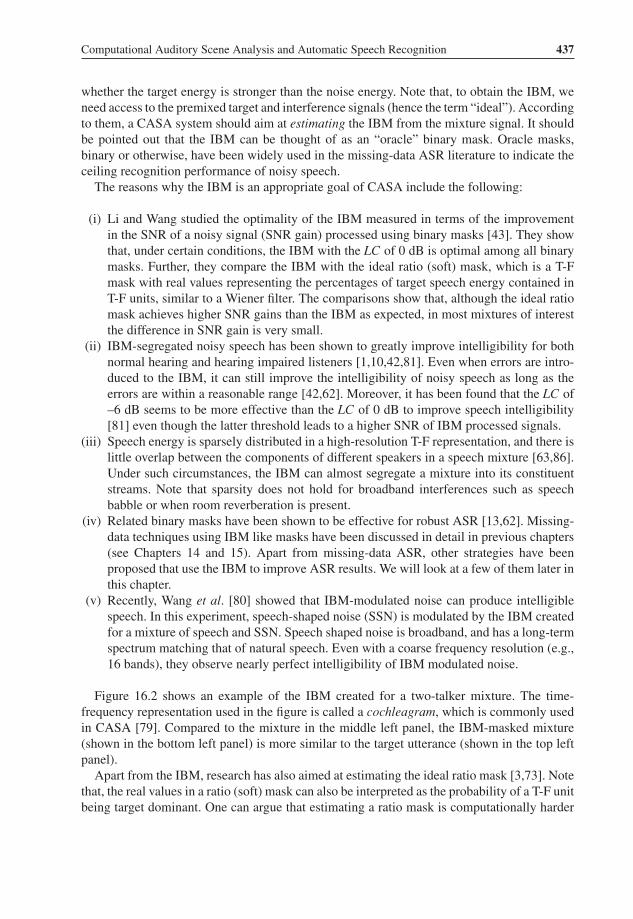
(iii) Speech energy is sparsely distributed in a high-resolution T-F representation, and there islittle overlap between the components of different speakers in a speech mixture [63,86].Under such circumstances, the IBM can almost segregate a mixture into its constituentstreams. Note that sparsity does not hold for broadband interferences such as speechbabble or when room reverberation is present.

(iv) Related binary masks have been shown to be effective for robust ASR [13,62]. Missing-data techniques using IBM like masks have been discussed in detail in previous chapters(see Chapters 14 and 15). Apart from missing-data ASR, other strategies have beenproposed that use the IBM to improve ASR results. We will look at a few of them later inthis chapter.

(v) Recently, Wang et al. [80] showed that IBM-modulated noise can produce intelligiblespeech. In this experiment, speech-shaped noise (SSN) is modulated by the IBM createdfor a mixture of speech and SSN. Speech shaped noise is broadband, and has a long-termspectrum matching that of natural speech. Even with a coarse frequency resolution (e.g.,16 bands), they observe nearly perfect intelligibility of IBM modulated noise.

Figure 16.2 shows an example of the IBM created for a two-talker mixture. The time-frequency representation used in the figure is called a cochleagram, which is commonly usedin CASA [79]. Compared to the mixture in the middle left panel, the IBM-masked mixture(shown in the bottom left panel) is more similar to the target utterance (shown in the top leftpanel).

Apart from the IBM, research has also aimed at estimating the ideal ratio mask [3,73]. Notethat, the real values in a ratio (soft) mask can also be interpreted as the probability of a T-F unitbeing target dominant. One can argue that estimating a ratio mask is computationally harder



Freq

uenc

y (H

z)

Target

0 2.5

8000

3278

1306

425

50

Freq

uenc

y (H

z)

Interference

0 2.5

8000

3278

1306

425

50

Freq

uenc

y (H

z)

Mixture

0 2.5

8000

3278

1306

425

50Time (s)

Freq

uenc

y (H

z)

Ideal binary mask

0 2.5

8000

3278

1306

425

50

Time (s)

Freq

uenc

y (H

z)

Masked mixture

0 2.5

8000

3278

1306

425

50

Figure 16.2 Illustration of the IBM. The top left panel shows a cochleagram of a target utterance wherebrightness indicates energy. The top right panel shows a cochleagram of the interference signal. Themiddle left panel shows a cochleagram of the mixture. The middle right panel shows the ideal binarymask for the mixture where a white pixel indicates 1 and a black pixel 0. The bottom left panel showsthe cochleagram of the IBM-masked mixture.

than estimating a binary mask [77]. Nevertheless, the use of ratio masks has been shown to beadvantageous in some ASR studies [3,73].

16.3.2 Typical CASA Architecture

Figure 16.3 shows a typical architecture of CASA. All CASA systems start with a peripheralanalysis of the acoustic input (the mixture). Typically, the peripheral analysis converts the signalinto a time-frequency representation. This is usually accomplished by using an auditory filterbank. The most commonly used is the gammatone filter bank [58]. The center frequencies ofthe gammatone filter bank are uniformly distributed on the ERB-rate scale [18]. ERB refers tothe equivalent rectangular bandwidth of an auditory filter, which corresponds to the bandwidth



Figure 16.3 Schematic diagram of a typical CASA system.

of an ideal rectangular filter that has the same peak gain as the auditory filter with the samecenter frequency and passes the same total power for white noise. Similar to the Bark scale, theERB-rate scale is a warped frequency scale akin to that of human cochlear filtering. The ERBscale is close to linear at low frequencies, but logarithmic at high frequencies. Figure 16.4shows the responses of eight such filters, uniformly distributed according to the ERB-ratescale from 100 to 2000 Hz. Although eight filters are sufficient to fully span a frequency rangeof 50–8000 Hz, more filters (32 or 64) are typically used for a better frequency resolution.To simulate the firing activity of auditory nerve fibers, the output from the gammatone filterbank is further subjected to some nonlinear processing, where the Meddis hair cell modelis typically used [48]. It models the rectification, compression and the firing pattern of the

0 10 20 30 40 50

100

203

339

518

753

1061

1467

2000

Cha

nnel

cen

ter

freq

uenc

y (H

z)

Time (ms)0 1000 2000 3000

−60

−50

−40

−30

−20

−10

0

Mag

nitu

de (

dB)

Frequency (Hz)

Figure 16.4 A gammatone filter bank. The left panel shows impulse responses of eight gammatonefilters, with center frequencies equally spaced between 100 Hz and 2 KHz on the ERB-rate scale. Theright panel shows the corresponding magnitude responses of the filters.



auditory nerve. Alternatively, a simple half wave rectification followed by some compression(square root or cubic root) can be used to model the nonlinearity. Finally, the output at eachchannel is windowed or downsampled. The result is the cochleagram of the acoustic signal asit models the processing performed by the cochlea [79]. An element of a cochleagram is a T-Funit, which represents the response of a particular filter at a time frame.

The next few stages vary depending on the specifics of different CASA systems. Thefeature extraction stage computes features such as F 0, onset/offset, amplitude and frequencymodulation. The extracted features enable the system to form segments, each of which is acontiguous region of T-F units. Segments provide a mid-level representation on which groupingoperates. The grouping stage utilizes primitive and schema-based grouping cues. The outputof the grouping stage can be an estimated binary mask or a ratio mask. Efficient algorithmsexist that can resynthesize the target signal using a T-F mask and the original mixture signal[79,82].

16.4 CASA Strategies

Given the goal of estimating the IBM, we now discuss strategies to achieve it. The mainfocus of this section will be on monaural CASA techniques which have seen most of thedevelopment.

Monaural source segregation uses a single recording of the acoustic scene from which thetarget is to be segregated. The most important cue utilized for this task is the fundamentalfrequency. F0 estimation from clean speech is fairly accurate and many systems exist thatperform well; for example Praat is a freely available tool which is widely used [6]. Thepresence of multiple sound sources in a scene adds to the complexity of the task as a singleframe may now have multiple pitch points. Perhaps the earliest system that used F0 for speechsegregation was proposed by Parsons [57]. He used the short-term magnitude spectrum of noisyspeech to estimate multiple F0s. A sub-harmonic histogram method, proposed by Shroeder[64], was used to estimate the most dominant F 0 in a frame. He then removed the harmonicsof the estimated F 0 from the mixture spectrum and used the remainder to estimate the secondF 0. The estimated F 0s were finally used to segregate the mixture.

We start our discussion on IBM estimation in Section 16.4.1 by introducing strategiesbased on noise-estimation techniques from the speech-enhancement literature. More recentCASA-based strategies aim to segregate the target by extracting ASA cues like F 0, amplitudemodulation and onset/offset, which are then used to estimate the IBM. An alternative approachis to treat mask estimation as a binary classification problem. We explain these approaches inthe subsequent subsections by treating two recent strategies in detail. The second subsectionfocuses on the tandem algorithm proposed by Hu and Wang [26] that uses several ASA cues toestimate the IBM. Section 16.4.3 focuses on a binary classification-based approach proposedby Kim et al. [36]. The final subsection briefly touches upon binaural CASA strategies.

16.4.1 IBM Estimation Based on Local SNR Estimates

In this sub-section, we discuss mask estimation strategies that are based on local signal-to-noise ratio estimates at each time-frequency unit. Such techniques typically make use of an



estimate of the short-time noise power spectrum. The estimated noise power can be used toobtain the SNR and in turn a T-F mask. It should be clear from Equation (16.1) that with thetrue local SNR information, the IBM can be readily calculated. The noise estimate can also beused to define masks based on alternative criteria, like the negative energy criterion used byEl-Maliki and Drygajlo [17]. We will first review a few noise-estimation techniques, followedby a brief discussion on how they can be used to estimate the IBM.

Noise (and SNR) estimation is a widely studied topic in speech enhancement largely inthe context of spectral subtraction [5]. One commonly used technique is to assume that noiseremains stationary throughout the duration of an utterance and that the first few frames are‘noise-only’. A noise estimate is then obtained by simply averaging the spectral energy ofthese frames. Such estimates are, for instance, used in Vizinho et al. [75], Josifovski et al.[34], Cooke et al. [13]. But noise is often nonstationary and therefore, such methods oftenresult in poor IBM estimates. More sophisticated techniques have been proposed to estimatenoise in nonstationary conditions. See, for example, voice-activity detection (VAD) [69] basedmethods [40], Hirsch’s histogram based methods [23], recursive noise-estimation techniques[23], etc. Seltzer et al. [65] use an approach similar to Hirsch’s to estimate the noise floor ineach sub-band, which is in turn used for mask estimation (see Section 16.4.3). A more detaileddiscussion on noise estimation can be found in Chapter 4.

All noise-estimation techniques can be easily extended to estimate the SNR at each T-F unitby using it to obtain an estimate of the clean speech power spectrum. A spectral subtractionbased approach [5,7] is commonly used, wherein the speech power is obtained by subtractingthe noise power from the observed noisy spectral power. Further, a spectral floor is set and anyestimate lower than the floor is automatically rounded to this preset value. Other direct SNR-estimation techniques have also been proposed in the literature. For example, Nemer et al.[53] utilize higher order statistics of speech and noise to estimate the local SNR, assuminga sinusoidal model for band restricted speech and a Gaussian model for noise. A supervisedSNR-estimation technique was proposed by Tchorz and Kollmeier [74]. They use featuresinspired from psychoacoustics and a multilayer perceptron (MLP)-based classifier to estimatethe SNR at each T-F unit. Interested readers are also referred to Loizou[46] for detailed reviewson these topics.

If a noise estimate is used to calculate the SNR, the IBM can be estimated using Equation(16.1) after setting the LC to an appropriate value. Although 0 dB is a natural choice here,other values have also been used [13,60]. Soft (ratio) masks can be obtained from local SNRestimates by applying a sigmoid function that maps it to a real number in the range [0, 1],thereby allowing it to be interpreted as probability measures for subsequent processing. Onecan also define masks based on a posteriori SNR, which is the ratio of the noisy signal powerto noise power expressed in dB [61]. This circumvents the need to estimate the clean speechpower and local SNR. Note that any a posteriori SNR criterion can be equivalently expressedusing a local SNR criterion. An even simpler alternative is to use the negative energy criterionproposed by El-Maliki and Drygajlo [17]. They identify reliable speech dominant units asthose T-F units for which the observed noisy spectral energy is greater than the noise estimate.In other words, T-F units for which the spectral energy after subtracting the noise estimate fromthe observed noisy spectral energy is negative are considered noise dominant and unreliable.Raj and Stern [59] note that a combination of an SNR criterion and a negative energy criterionusually yields better quality masks.



In practice, such noise-estimation-based techniques work well in stationary conditions buttend to produce poor results in nonstationary conditions. Nonetheless, SNR-based techniquesare still used because of their simplicity.

16.4.2 IBM Estimation using ASA Cues

The tandem system by Hu and Wang [26] aims at voiced speech segregation and F0 estimationin an iterative fashion. In describing the algorithm, we will explain how some of the ASA cuescan be extracted and utilized for computing binary masks.

The tandem system uses several auditory representations that are widely used for pitchestimation. These representations are based on autocorrelation, which was originally proposedby Licklider back in the 1950s to explain pitch perception [44]. Autocorrelation has been usedby other F 0 estimation techniques [24,38,85]. The tandem system first uses a gammatonefilter bank to decompose the signal into 128 frequency channels with center frequenciesspaced uniformly in the ERB-rate scale from 50 to 8000 Hz. The output at each channel isdivided into frames of length 20 ms with 10 ms overlap. A running autocorrelation function(ACF) is then calculated according to Equation (16.2) at each frame to form a correlogram:

A(t, f, τ ) =

∑n

x(tTt − nTn , f )x(tTt − nTn − τTn , f )√∑n

x2(tTt − nTn , f )√∑

n

x2(tTt − nTn − τTn , f ). (16.2)

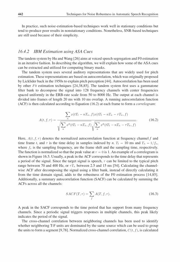
Here, A(t, f, τ ) denotes the normalized autocorrelation function at frequency channel f andtime frame t, and τ is the time delay in samples indexed by n. Tt = 10 ms and Tn = 1/fs ,where fs is the sampling frequency, are the frame shift and the sampling time, respectively.The function is normalized so that the peak value at τ = 0 is 1. An example of a correlogram isshown in Figure 16.5. Usually, a peak in the ACF corresponds to the time delay that representsa period of the signal. Since the target signal is speech, τ can be limited to the typical pitchrange between 70 and 400 Hz, or τTn between 2.5 and 15 ms [54]. Calculating the channel-wise ACF after decomposing the signal using a filter bank, instead of directly calculating itfrom the time domain signal, adds to the robustness of the F0 estimation process [14,85].Additionally, a summary autocorrelation function (SACF) can be calculated by summing theACFs across all the channels:

SACF (T, τ ) =∑f

A(T, f, τ ). (16.3)

A peak in the SACF corresponds to the time period that has support from many frequencychannels. Since a periodic signal triggers responses in multiple channels, this peak likelyindicates the period of the signal.

The cross-channel correlation between neighboring channels has been used to identifywhether neighboring T-F units are dominated by the same source which can be used to groupthe units to form a segment [9,78]. Normalized cross-channel correlation, C(t, f ), is calculated



50

332

839

1919

3864

8000Fr

eque

ncy

(Hz)

0 4 8 12Delay (ms)

0 150

332

839

1919

3864

8000

0 4 8 12Delay (ms)

0 1

(a)

0 4 8 1250

332

839

1919

3864

8000

Freq

uenc

y (H

z)

Delay (ms)0 1 0 4 8 12

50

332

839

1919

3864

8000

Delay (ms)0 1

(b)

Figure 16.5 Autocorrelation and cross-channel correlation. (a) Correlogram at a frame for clean speech(top left panel) and a mixture of speech with babble noise at 6 dB SNR (top right panel). The corre-sponding cross-channel correlation and summary autocorrelation are shown on the right and the bottompanel of each figure, respectively. A peak in the SACF is clearly visible in both cases. Note that corre-lations of different frequency channels are represented using separate lines. (b) Corresponding envelopecorrelogram and envelope cross-channel correlation for clean speech (bottom left panel) and the mixture(bottom right panel). It can be clearly seen that the functions estimated from clean speech and noisyspeech match closely.

using the ACF as:

C(t, f ) =

∑τ

[A(t, f, τ ) − A(t, f )

] [A(t, f + 1, τ ) − A(t, f + 1)

]√∑

τ

[A(t, f, τ ) − A(t, f )

]2√∑

τ

[A(t, f + 1, τ ) − A(t, f + 1)

]2. (16.4)

Here, A(t, f ) denotes the mean of the ACF function over τ .



As mentioned earlier, gammatone filters with higher center frequencies have wider band-widths (see Figure 16.4). As a result, for a periodic signal, high-frequency filters will respondto more than one harmonic of the signal. These harmonics are referred to as unresolved.Unresolved harmonics cause filter responses to be amplitude modulated, and the envelope ofa filter response fluctuates at the fundamental frequency of the signal. This property has alsobeen used as a cue to group segments and units in high-frequency channels [24]. Amplitudemodulation or envelope can be captured by half wave rectification followed by band-passfiltering of the response. The pass band of the filter corresponds to the plausible pitch range ofthe signal. Replacing the filter responses in Equation (16.2) and Equation (16.4) with the ex-tracted envelopes yields the normalized envelope autocorrelation, AE(t, f, τ ), and the envelopecross-channel correlation, CE(t, f ), respectively. AE can be used to estimate the periodicityof amplitude fluctuation. CE encodes the similarity of the response envelopes of neighboringchannels and aids segmentation. Figure 16.5 shows an example of a correlogram and an en-velope correlogram for a single frame of speech (clean and noisy), and their correspondingcross-channel correlations and SACFs.

For T-F unit labeling, the tandem algorithm uses the probability that the signal within a unitis in agreement with a pitch period τ . This probability, denoted as P (T, f, τ ), is estimated withthe help of an MLP using a six-dimensional (6-D) pitch-based feature vector:

r(t, f, τ ) = [A(t, f, τ ), f (t, f )τ − int(f (t, f )τ ), int(f (t, f )τ ),

AE(t, f, τ ), fE(t, f )τ − int(fE(t, f )τ ), int(fE(t, f )τ )], (16.5)

where the vector consists of ACFs and features derived using an estimate of the averageinstantaneous frequency, f (t, f ). In the equation, int(.) returns the nearest integer and thesubscript ‘E’ denotes envelope. fE is the instantaneous frequency estimated from the responseenvelope. If a signal is harmonically related to the pitch period τ , then int(f (t, f )τ ) andint(fE(t, f )τ ) will indicate a harmonic number. The difference between these products andtheir nearest integers in the second and the fourth terms quantifies a degree of this relationship.An MLP is trained for each filter channel in order to estimate P (t, f, τ )1.

The algorithm first estimates initial pitch contours, each of which is a set of contiguouspitch periods belonging to the same source, and their associated binary masks for up to twosound sources. The main part of the algorithm iteratively refines the initial estimates. The finalstage applies onset/offset analysis to further improve segregation results. Let us now look atthese stages in detail.

The initial stage starts by identifying T-F units corresponding to periodic signals. Suchunits tend to have high cross-channel correlation or envelope cross-channel correlation and,therefore, are identified by comparing C(t, f ) and CE(t, f ) with a threshold. Within each frame,the algorithm considers up to two dominant voiced sound sources. The identified T-F units ofa frame are grouped using a two step process. First, estimate up to two F 0s. Next, assign a T-Funit to an F 0 group if it agrees with the F 0.

An earlier model by Hu and Wang [24] identifies the dominant pitch period of a frame asthe lag that corresponds to the maximum in the summary autocorrelation function (Equation(16.3)). To check if a T-F unit agrees with the dominant pitch period, they compare the value

1 Note that this term is a convenient abuse of notation. It, in fact, represents the posterior probability of the T-F unitbeing in agreement with the pitch period given the 6-D pitch-based features.



of the ACF at the estimated pitch period to the peak value of the ACF for that T-F unit:

A(t, f, τD (t))A(t, f, τP (t, f ))

> θP . (16.6)

Here, τD (t) and τP (t, f ) are the delays that correspond to the estimated F 0 and the maximumin the ACF, respectively, for channel f at time frame t. If the signal within the T-F unit has aperiod close to the estimated F 0, then this ratio will be close to 1. θP defines a threshold tomake a binary decision about the agreement.

The tandem algorithm uses a similar approach, but instead of the ACF it uses the probabilityfunction, P (t, f, τ ), estimated using the MLPs. Having identified the T-F units of each framewith strong periodicity, the algorithm chooses the lag, τ , that has the most support from theseunits as the dominant pitch period of the frame. A T-F unit is said to support τ if the probability,P (t, f, τ ), is above a chosen threshold. The T-F units that support the dominant pitch periodare then grouped together. The second pitch period and the associated set of T-F units areestimated in a similar fashion, using those units not in the first group. To remove spuriouspitch estimates, if there are too few supporting T-F units, the estimated pitch is discarded.

To form pitch contours from these initial estimates, the algorithm groups the pitch periodsof any three consecutive frames if their values change by less than 20% from one frame to thenext. The temporal continuity of the sets of T-F units associated with the pitch periods is alsoconsidered before grouping pitch estimates together; at least half of the frequency channelsassociated with the pitch periods of neighboring frames should match for them to be groupedinto a pitch contour. After the initial stage, each pitch contour has an associated T-F mask.Since pitch changes rather smoothly in natural speech, each of the formed pitch contours andits associated binary mask usually belong to a single sound source. Isolated pitch points afterthis initial grouping are considered unreliable and discarded.

These initial estimates are then refined using an iterative procedure. The idea is to useobtained binary masks to obtain better pitch contours, and then use the refined pitch estimatesto re-estimate the masks. Each iteration of the tandem algorithm consists of two steps:

(i) The first step expands each pitch contour to its neighboring frames, and re-estimates itspitch periods. Since pitch changes smoothly over time, the pitch periods of the contourcan be used to estimate potential pitch periods in the contour’s neighboring frames.Specifically, for the kth pitch contour τk , that extends from frame t1 to t2 , the correspondingbinary mask, Mk (t) (t = t1 , . . . , t2), is extended to frames t1 − 1 and t2 + 1 by settingMk (t1 − 1) = Mk (t1) and Mk (t2 + 1) = Mk (t2). Using this new mask, the periods of thepitch contour are reestimated. A summary probability function, SP (t, τ ), which is similarto SACF (t, τ ) but uses P (t, f, τ ) values instead of A(t, f, τ ), is calculated at each framefor this purpose. The SP function tends to have significant peaks at multiples of the pitchperiod. Therefore, an MLP is trained to choose the correct pitch period from among themultiple candidates. The expansion stops at either end when the estimated pitch violatestemporal continuity with the existing pitch contour. Note that, as a result of contourexpansion, pitch contours may be combined.

(ii) The second step reestimates the mask corresponding to each of the pitch contours. Thisis done by identifying T-F units of each frame that are in agreement with the estimatedpitch period of that frame. Given the pitch period τD (t), P (t, f, τD ) can be directly used tomake this decision at each T-F unit. But this does not take into consideration the temporal



continuity and the wide-band nature of speech. If a T-F unit is in agreement with τD ,its neighboring T-F units also tend to agree with τD . For added robustness, the tandemalgorithm trains an MLP to perform unit labeling based on a neighboring set of T-F units.It takes as input the P (t, f, τ ) values of a set of neighboring T-F units, centered at the unitfor which the labeling decision has to be made. The output of this MLP is finally used tolabel each T-F unit.

The algorithm iterates between these two steps until it converges or the number of iterationsexceeds a predefined maximum (20 is suggested).

The final step of the tandem algorithm is a segmentation stage based on onset/offset analysis,which may be viewed as post processing. The stage forms segments by detecting suddenchanges in intensity as such a change indicates an onset or offset of an acoustic event. Asdiscussed earlier, onset and offset are prominent ASA principles (see Figure 16.1). Segmentsare formed using multiscale analysis of onsets and offsets (see Hu and Wang [25] for details).The tandem algorithm further breaks each segment down to channel wise subsegments, calledT-segments as they span multiple time frames but are restricted to a single frequency channel.Each T-segment is then classified as a whole as target dominant if at least half its energy iscontained in the voiced frames of the target and at least half of the energy in these voicedframes is included in the target mask. If the conditions are not satisfied, the labeling from theiterative stage remains unchanged for the units of the T-segment.

Figure 16.6 illustrates the results of different stages of the tandem system. The maskobtained at the end of the iterative stage (Figure 16.6(e)) includes most of the target speech. Thesubsequent segmentation stage improves the segregation results by recovering a few previouslymasked (mask value 0) T-F units, for example toward the end of the utterance in Figure 16.6(g).These units were identified from the onset/offset segments. The final resynthesized waveform,shown in Figure 16.6(h), is close to the original signal (Figure 16.6(b)).

There are two important aspects of CASA that the tandem algorithm does not consider.The first one is sequential organization. The outputs of the tandem system are multiple pitchcontours and associated binary masks. The pitch track (and therefore the mask) of a targetutterance need not be continuous as there are breaks due to silence and unvoiced speech.Sections before and after such discontinuities have to be sequentially grouped into the targetstream. The tandem system assumes ideal sequential grouping, and therefore ignores thesequential grouping issue. Methods for sequential grouping have been proposed. Barker et al.[4] proposed a schema based approach using ASR models to simultaneously perform sequentialintegration and speech recognition (more about this in Section 14.4.3). Ma et al. [47] laterused a similar approach to group segments that were formed using correlograms in voicedintervals and a watershed algorithm in unvoiced intervals. Shao and Wang [67] proposed aspeaker model-based approach for sequential grouping. Recently, Hu and Wang [30] proposedan unsupervised grouping strategy based on clustering and reported results comparable to themodel-based approach of Shao and Wang.

The second issue with the tandem algorithm is that it does not deal with unvoiced speech.An analysis by Hu and Wang [28] shows that unvoiced speech accounts for more than 20%of spoken English, measured in terms of both frequency and duration of speech sounds.Therefore, unvoiced speech segregation is important for improving the intelligibility andASR of the segregated target signal. Dealing with unvoiced speech is challenging as it hasnoise-like characteristics and lacks strong grouping cues such as F 0. Hu and Wang [28]



8000

3255

1246

363

500 0.5 1 1.5 2 2.5

Freq

uenc

y (H

z)(a)

0 0.5 1 1.5 2 2.5

(b)

8000

3255

1246

363

500 0.5 1 1.5 2 2.5

Freq

uenc

y (H

z)

(c)0 0.5 1 1.5 2 2.5

(d)8000

3255

1246

363

500 0.5 1 1.5 2 2.5

Freq

uenc

y (H

z)Fr

eque

ncy

(Hz)

Freq

uenc

y (H

z)

Am

plitu

deA

mpl

itude

Am

plitu

deA

mpl

itude

Am

plitu

de

(e)0 0.5 1 1.5 2 2.5

(f)

8000

3255

1246

363

500 0.5 1 1.5 2 2.5

(g)0 0.5 1 1.5 2 2.5

(h)

8000

3255

1246

363

500 0.5 1 1.5 2 2.5

Time (s) Time (s)

(i)

0 0.5 1 1.5 2 2.5

(j)

Figure 16.6 Different stages of IBM estimation using the tandem system. (a) Cochleagram of a femaletarget utterance. (b) Corresponding waveform. (c) Cochleagram of a mixture signal obtained by addingcrowd noise to the target utterance. (d) Corresponding waveform. (e) Mask obtained at the end ofthe iterative stage of the algorithm. (f) Waveform of the resynthesized target using the mask. (g) Thefinal mask obtained after the segmentation stage. (h) The resynthesized waveform. (i) The IBM. (j)Resynthesized signal using the IBM. Reproduced by permission from Hu and Wang [26] © 2010 IEEE.

suggest a method to extract unvoiced speech using onset/offset based segments. They firstsegregate voiced speech. Then, acoustic-phonetic features are used to classify the remainingsegments as interference dominant or unvoiced speech dominant. A simpler system was laterproposed by Hu and Wang [29]. Their system first segregates voiced speech and removesother periodic intrusions from the mixture. It then uses a spectral subtraction based scheme



to obtain segments in unvoiced intervals (an unvoiced interval corresponds to a contiguousgroup of unvoiced frames); the noise estimate for each unvoiced interval is estimated usingthe mixture energy in the masked T-F units of its neighboring voiced intervals. Together withan approximation of the target energy obtained by subtracting the estimated noise from themixture, the local SNR at each T-F unit is calculated. The segments themselves are formed bygrouping together neighboring T-F units that have estimated SNRs above a chosen threshold.The obtained segments are then classified as target or interference dominant based on theobservation that most of the target dominant unvoiced speech segments reside in the high-frequency region. The algorithm works well if the noise remains fairly stationary during theduration of an unvoiced interval and the neighboring voiced intervals.

16.4.3 IBM Estimation as Binary Classification

The tandem algorithm exemplifies a system that uses ASA cues and supervised learning toestimate the IBM. When it comes to direct classification, the issues lie in choosing appropriatefeatures that can discriminate target speech from interference, and an appropriate classifier.To explain how direct classification is applied, we describe the classification-based approachof Kim et al. [36] in detail.

The system by Kim et al. uses amplitude modulation spectrograms (AMS) as the feature tobuild their classifier. To obtain AMS features, the signal is first passed through a 25 channelfilter bank, with filter center frequencies spaced according to the mel-frequency scale. Theoutput at each channel is full-wave rectified and decimated by a factor of 3 to obtain theenvelope of the response. Next, the envelope is divided into frames 32 ms long with 16 msoverlap. The modulation spectrum at each T-F unit is then calculated using the FFT2. TheFFT magnitudes are finally integrated using 15 triangular windows spaced uniformly from15.6 to 400 Hz, resulting in 15 AMS features [39]. Kim et al. augment the extracted AMSfeatures with delta features calculated from the neighboring T-F units. The delta features arecalculated across time and frequency, and for each of the 15 features separately. They helpcapture temporal and spectral correlations between T-F units. This creates a 45-dimensionalfeature representation for each T-F unit, AMS(t, f ).

Given the 45-dimensional input, a Gaussian mixture model (GMM)-based classifier istrained to do the classification. The desired unit labels are set using the IBM created usingan LC (see Equation (16.1)) of –8 dB for low-frequency channels (channels 1 through 15)and –16 dB for high-frequency channels (channels 16 through 25). This creates a group ofmasked T-F units, represented as λ0 , and unmasked (mask value 1) T-F units, λ1 . The authorschose a lower LC for high-frequency channels to account for the difference in the maskingcharacteristics of speech across spectrum. Each group, λi , where i = 0, 1, is further divided intotwo smaller subgroups, λ0

i and λ1i , using a second threshold, LCi . The thresholds (LC0 < LC

and LC1 > LC) are chosen such that the amount of training data in the two subgroups ofa group are the same. This second subdivision is done mainly to reduce the training timeof the GMMs. A 256-mixture, 45-dimensional, full-covariance GMM is trained using theexpectation-maximization algorithm to model the distribution of each of the 4 subgroups.

2 A T-F unit, here, refers to a 32 ms long frame at a particular frequency channel.



Given a T-F unit from a noisy utterance, a Bayesian decision is then made to obtain a binarylabel that is 0 if and only if P (λ0 | AMS(t, f )) > P (λ1 | AMS(t, f )), where

P (λ0 | AMS(t, f )) =P (λ0 , AMS(t, f ))

P (AMS(t, f ))

=P (λ0

0)P (AMS(t, f ) | λ00) + P (λ1

0)P (AMS(t, f ) | λ10)

P (AMS(t, f )).

The equation calculates the a posteriori probability of λ0 given the AMS features at the T-Funit. P (λ0

0) and P (λ10) are the a priori probabilities of subgroups λ0

0 and λ10 , respectively,

calculated from the training set. The likelihoods, P (AMS(t, f ) | λ00) and P (AMS(t, f ) | λ1

0),are estimated using the trained GMMs. P (AMS(t, f )) is independent of the class label and,hence, can be ignored. P (λ1 | AMS(t, f )) is calculated in a similar fashion.

One advantage of using the AMS feature is that it can handle both voiced and unvoicedspeech, as opposed to the 6-D pitch based feature used by the tandem algorithm which can beused only to classify voiced speech. As a result, the mask obtained using Kim et al.’s algorithmincludes both voiced and unvoiced speech.

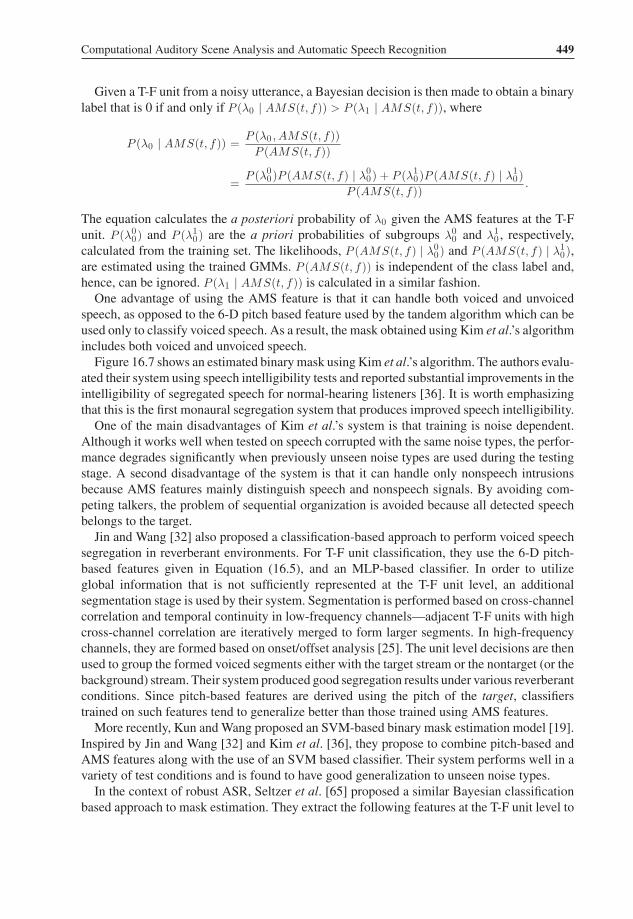
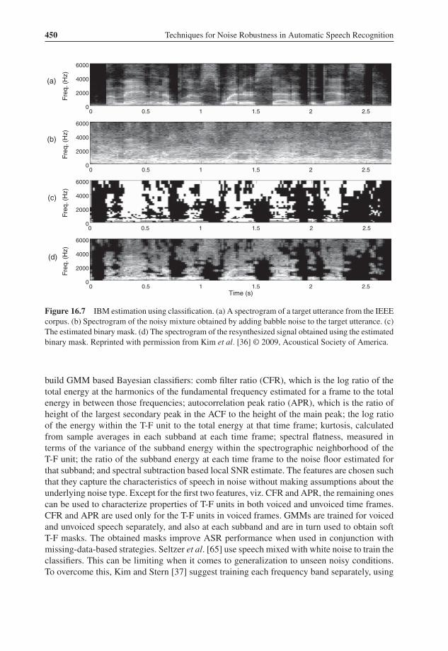
Figure 16.7 shows an estimated binary mask using Kim et al.’s algorithm. The authors evalu-ated their system using speech intelligibility tests and reported substantial improvements in theintelligibility of segregated speech for normal-hearing listeners [36]. It is worth emphasizingthat this is the first monaural segregation system that produces improved speech intelligibility.

One of the main disadvantages of Kim et al.’s system is that training is noise dependent.Although it works well when tested on speech corrupted with the same noise types, the perfor-mance degrades significantly when previously unseen noise types are used during the testingstage. A second disadvantage of the system is that it can handle only nonspeech intrusionsbecause AMS features mainly distinguish speech and nonspeech signals. By avoiding com-peting talkers, the problem of sequential organization is avoided because all detected speechbelongs to the target.

Jin and Wang [32] also proposed a classification-based approach to perform voiced speechsegregation in reverberant environments. For T-F unit classification, they use the 6-D pitch-based features given in Equation (16.5), and an MLP-based classifier. In order to utilizeglobal information that is not sufficiently represented at the T-F unit level, an additionalsegmentation stage is used by their system. Segmentation is performed based on cross-channelcorrelation and temporal continuity in low-frequency channels—adjacent T-F units with highcross-channel correlation are iteratively merged to form larger segments. In high-frequencychannels, they are formed based on onset/offset analysis [25]. The unit level decisions are thenused to group the formed voiced segments either with the target stream or the nontarget (or thebackground) stream. Their system produced good segregation results under various reverberantconditions. Since pitch-based features are derived using the pitch of the target, classifierstrained on such features tend to generalize better than those trained using AMS features.

More recently, Kun and Wang proposed an SVM-based binary mask estimation model [19].Inspired by Jin and Wang [32] and Kim et al. [36], they propose to combine pitch-based andAMS features along with the use of an SVM based classifier. Their system performs well in avariety of test conditions and is found to have good generalization to unseen noise types.

In the context of robust ASR, Seltzer et al. [65] proposed a similar Bayesian classificationbased approach to mask estimation. They extract the following features at the T-F unit level to



Freq

. (H

z)

0 0.5 1 1.5 2 2.50

2000

4000

6000Fr

eq. (

Hz)

0 0.5 1 1.5 2 2.50

2000

4000

6000

Freq

. (H

z)

0 0.5 1 1.5 2 2.50

2000

4000

6000

Freq

. (H

z)

Time (s)0 0.5 1 1.5 2 2.5

0

2000

4000

6000

(b)

(a)

(c)

(d)

Figure 16.7 IBM estimation using classification. (a) A spectrogram of a target utterance from the IEEEcorpus. (b) Spectrogram of the noisy mixture obtained by adding babble noise to the target utterance. (c)The estimated binary mask. (d) The spectrogram of the resynthesized signal obtained using the estimatedbinary mask. Reprinted with permission from Kim et al. [36] © 2009, Acoustical Society of America.

build GMM based Bayesian classifiers: comb filter ratio (CFR), which is the log ratio of thetotal energy at the harmonics of the fundamental frequency estimated for a frame to the totalenergy in between those frequencies; autocorrelation peak ratio (APR), which is the ratio ofheight of the largest secondary peak in the ACF to the height of the main peak; the log ratioof the energy within the T-F unit to the total energy at that time frame; kurtosis, calculatedfrom sample averages in each subband at each time frame; spectral flatness, measured interms of the variance of the subband energy within the spectrographic neighborhood of theT-F unit; the ratio of the subband energy at each time frame to the noise floor estimated forthat subband; and spectral subtraction based local SNR estimate. The features are chosen suchthat they capture the characteristics of speech in noise without making assumptions about theunderlying noise type. Except for the first two features, viz. CFR and APR, the remaining onescan be used to characterize properties of T-F units in both voiced and unvoiced time frames.CFR and APR are used only for the T-F units in voiced frames. GMMs are trained for voicedand unvoiced speech separately, and also at each subband and are in turn used to obtain softT-F masks. The obtained masks improve ASR performance when used in conjunction withmissing-data-based strategies. Seltzer et al. [65] use speech mixed with white noise to train theclassifiers. This can be limiting when it comes to generalization to unseen noisy conditions.To overcome this, Kim and Stern [37] suggest training each frequency band separately, using



artificial colored noise signals generated specifically for each band. They show that this canyield better generalization results as compared to using white noise alone for training.

In a way, classification-based strategies simplify the task of speech segregation, at leastconceptually. It bypasses the steps of a typical CASA system which extracts perceptuallymotivated cues and applies the ASA stages of segmentation and grouping to obtain a binarymask. The potential downside of relying on supervised learning is the perennial issue ofgeneralization to unseen conditions.

16.4.4 Binaural Mask Estimation Strategies

Binaural CASA systems use two microphone recordings to segregate the target from the mix-ture. Most binaural systems try to extract localization cues, for example azimuth, which areencoded in the differences between the signals that reach the two ears (or microphones). Inthis regard, interaural time difference (ITD) and interaural intensity difference (IID) are thetwo most important cues. ITD is the difference between the arrival times of the signal at thetwo ears. ITD is ambiguous at high frequencies (> 1.5 KHz) because of short wavelengthsas compared to the distance between the ears. IID is the difference in the intensity of thesound that reaches the two ears, usually expressed in decibels, and it occurs because of the‘shadow’ effect of the human head. Contrary to ITD, IID is not useful at low frequencies(< 500 Hz) because such low-frequency sound components diffract around the head overcom-ing the shadow effect in the process.

Two classical strategies strongly influenced binaural segregation: the cross-correlation basedmodel for ITD estimation proposed by Jeffress [31] and the equalization-cancellation (EC)model of Durlarch [16]. The EC model tries to segregate the target in a two stage process.In the first stage, the noise levels in the signals arriving at the two ears are equalized. Thisis followed by subtraction of the signals at the two ears in the cancellation stage. The noiseequalized in the first stage gets canceled during the second stage, producing a cleaner target.The Jeffress model is based on the similarity of the signals that arrive at the two ears. Theneural firing patterns of the two ears are passed through delay lines; the delay that maximizesthe correlation between the two patterns is identified as the ITD of the signal.

To compute ITD, a normalized cross-correlation function, C(t, f, τ ), is typically used

C(t, f, τ ) =

∑n

xL (tTt − nTn , f )xR (tTt − nTn − τTn , f )√∑n

x2L (tTt − nTn , f )

√∑n

x2R (tTt − nTn − τTn , f )

. (16.7)

The above equation calculates cross-correlation at frequency channel f and time frame t, fora time lag τ . xL and xR correspond to the left and right ear response, respectively. Tt andTn have the same meanings as in Equation (16.2). Similar to the normalized autocorrelationfunction, the cross-correlation function will have a peak at a delay that relates to ITD. IID canbe calculated as the ratio of the mean power of the signals that arrive at the two ears:

IID(t, f ) = 10 log10

( ∑n x2

L (tTt − nTn , f )∑n x2

R (tTt − nTn , f )

). (16.8)



An IBM estimation strategy based on classifying ITD and IID estimates was proposed byRoman et al. [62], which is probably the first classification-based system for speech segrega-tion. They observed that, given a predefined configuration of the target and the interference(configuration here refers to the azimuths of the target and the interference), ITD and IIDvalues vary smoothly and systematically with respect to the relative strength of the targetand the mixture. This prompted them to model the distribution of target dominant units andinterference dominant units of each frequency channel in the ITD-IID space. Their systemmodels the distributions using a nonparametric kernel-density estimator. For an unseen testutterance, the binary decision at each T-F unit is made by comparing the probabilities of theunit being target dominant and interference dominant, given the observed ITD and IID at thatunit. The binary masks estimated by their model are very close to the IBM, with excellentperformances in terms of SNR gains, speech intelligibility and ASR accuracies. The maindrawback of the model is that ITD-IID distributions are configuration dependent. A similarsystem was proposed by Harding et al. [20], which assumes that only the target azimuth isknown a priori. It then learns the joint distribution of ITD and IID for target dominant T-Funits using a histogram-based method. These distributions are used to predict the probabilityof a unit being target dominant from the observed ITD and IID. The estimated probabilitiesare directly used in the form of a ratio mask, to improve ASR results in reverberant conditions.

The above strategies are based on modeling the distribution of the binaural cues in the ITD-IID space. An alternative approach was proposed by Palomaki et al. [55]. This approach firstestimates target and interference azimuths. It then classifies a T-F unit as target or interferencedominant by comparing the values of the cross-correlation function at the estimated azimuthsof the target and the interference. In order to deal with room reverberation, their system modelsthe precedence effect [45] by using the low-pass filtered envelope response of each channelas an inhibitor. This reduces the effect of late echoes in reverberant situations by preservingtransient and suppressing sustained responses. Palomaki et al. reported good ASR results inreverberant situations using the above algorithm to estimate binary masks.

Recently, Woodruff and Wang [84] proposed a system that combines monaural and binauralcues to estimate the IBM. Their system uses a monaural CASA algorithm to first obtain simul-taneous streams, each occupying a continuous time interval. They use the tandem algorithm,described earlier, for this purpose. Binaural cues are then used to jointly estimate the azimuthsof the streams that comprise the scene and their corresponding sets of sequentially groupedsimultaneous streams.

16.5 Integrating CASA with ASR

The CASA strategies discussed in Section 16.4 provide us several perceptually inspired waysof segregating the target from a mixture. The main focus has been on estimating the ideal binarymask. Although IBM-based strategies produce good segregation results, integrating CASA andASR has not been as straightforward a task as it seems. A simple way of combining CASAwith ASR is to use CASA as a preprocessor. ASR models trained in clean conditions canthen be used to perform recognition on the segregated target speech. This can be problematic.Even when the IBM is used, the resynthesized signal will have artifacts that may pose chal-lenges to recognition. Errors in IBM estimation will further degrade the performance of suchsystems.



Nevertheless, CASA has been used as a preprocessor in some systems and has been shownto produce good results. One such model was proposed by Srinivasan et al. [73]. Their systemuses a ratio T-F mask to enhance a noisy utterance. A conventional HMM-based ASR systemtrained using the mel-frequency cepstral coefficients (MFCC) of clean speech is used torecognize the enhanced speech. For mask estimation, they use the binaural segregation modelby Roman et al. [62]. Srinivasan et al. compared their system with the missing-data ASRapproach [13] and found that using such a CASA-based preprocessor can be advantageousas the vocabulary size of the recognition task increases. The limitation of missing-data ASRin dealing with larger vocabulary tasks had been reported earlier [60]. The use of a ratiomask instead of a binary mask coupled with accurate mask estimation helped their system inovercoming some of the limitations of using CASA as a preprocessor.

More recently, Hartmann and Fosler-Lussier [21] compared the performance of an ASRsystem that simply discards masked T-F units, which is equivalent to processing the noisyspeech with a binary mask, with a system that reconstructs those units based on the informationavailable from the unmasked T-F units. Such feature-reconstruction strategies have been usedto improve noise robust ASR [60]. An HMM based ASR system trained in clean conditionsis used to perform recognition. They observe that the direct use of IBM-processed speechperforms significantly better than the reconstructed speech, and yields ASR results only afew percentage points worse than those in clean conditions. When noise is added to the IBMby randomly flipping 1s and 0s, only after the amount of mask errors exceeds some pointdoes reconstruction work better. This is a surprising observation, considering the conventionalwisdom that the binary nature of a mask is supposed to skew the cepstral coefficients (theyused PLP cepstral coefficients to build their ASR system). This study points to the need of adeeper understanding of the effects of using binary masks on ASR performance.

The above methods somehow modify the features so that they can be used with ASRmodels trained in clean conditions. Such strategies have been called feature compensationor source-driven methods. Feature compensation includes techniques that use CASA basedstrategies for segregating the target [21,73] and reconstructing unreliable features [60]. Analternative approach would be to modify ASR models so that they implicitly accommodatemissing or corrupt speech features. Such strategies have been termed model compensation orclassifier compensation methods. The missing-data ASR techniques are examples of modelcompensation strategies [13]. There are also strategies that combine feature compensation andmodel compensation [15,71], and simultaneously perform CASA and ASR [4,72].

A much simpler strategy for integrating CASA and ASR was proposed by Narayanan andWang [50] and Karadogan et al. [35]. They interpret IBMs as binary images and use a binarypattern classifier to do ASR. The idea of using binary pattern recognition for ASR is radicallydifferent from the existing strategies that use detailed speech features like MFCCs. Their workwas motivated by the speech perception study showing that modulating noise by the IBMcan produce intelligible speech for humans [80, also see Section 16.3]. Since noise carries nospeech information, intelligibility must be induced by the binary pattern of the IBM itself.This indicates that the pattern carries important phonetic information. The system describedin Narayanan and Wang [50] is designed for an isolated digit recognition task. The ASRmodule is based on convolutional neural networks [41,68], which have previously been usedsuccessfully for handwritten digit and object recognition. Their system obtains reasonableresults even when the IBM is estimated directly from noisy speech using a CASA algorithm.They extend their system further in Narayanan and Wang [51] to perform a more challenging



phone classification task, and show that IBMs and traditional speech features like MFCCscarry complimentary information that can be combined to improve the overall classificationperformance. The combined system obtains classification accuracies that compare favorablyto most of the results reported in recent phone classification literature. It is quite interesting tonote that features that are based on binary patterns can obtain good results on complex ASRtasks. Such CASA inspired features may eventually be needed for achieving robust ASR.

In the following subsection we discuss in greater detail an example of a CASA-inspiredASR framework. The subsection focuses on the uncertainty transform model proposed bySrinivasan and Wang [71] that combines feature compensation and model compensation toimprove ASR performance.

16.5.1 Uncertainty Transform Model

Using a speech-enhancement algorithm to obtain features for ASR does not always yield goodrecognition results. This is because, even with the best enhancement algorithms, the enhancedfeatures remain somewhat noisy, as far as the ASR models trained in clean conditions areconcerned. Moreover, the variance of such features, with respect to the corresponding cleanfeatures, varies across time and frequency. Uncertainty decoding has been suggested as astrategy to modify ASR model parameters to take into account the inherent uncertainty ofsuch enhanced features (see Chapter 17 for a more detailed handling of uncertainty decodingstrategies). It has been shown that feature uncertainties contribute to an increase in the varianceof trained acoustic variables and accounting for it during the recognition (decoding) stage cansignificantly improve ASR performance [15].

A mismatch in the domain of operation between speech enhancement or segregation andASR can pose problems in effectively adjusting ASR model parameters based on estimateduncertainty. Such a mismatch exists for most CASA-based techniques as they operate eitherin the spectral or T-F domain, as opposed to ASR models that operate in the cepstral domain.Training ASR models in the spectral domain is known to produce suboptimal performance. Inorder to overcome this mismatch problem, Srinivasan and Wang [71] suggested a techniqueto transform the uncertainties estimated in the spectral domain to the cepstral domain.

The uncertainty transform model by Srinivasan and Wang consists of a speech-enhancementmodule, an uncertainty transformer, and a traditional HMM-based ASR module that operatesin the cepstral domain. The enhancement module uses a spectrogram reconstruction methodthat is similar to [60] but operates in the linear spectral domain. To perform recognition,the enhanced spectral features are transformed to the cepstral domain. The correspondinguncertainties, originally estimated in the spectral domain, are transformed using a supervisedlearning method. Given the enhanced cepstral features and associated uncertainties, recognitionis performed in an uncertainty decoding framework. Details about these stages are discussedbelow.

The speech-enhancement module starts by converting a noisy speech signal into the spectraldomain using the FFT. The noisy spectrogram is then processed using a speech-segregationalgorithm that estimates the IBM. A binary mask partitions a noisy spectral vector, y, into itsreliable components, yr , and the unreliable components, yu . Assuming that yr sufficientlyapproximates the corresponding clean speech spectral values, xr , the goal of reconstructionis to approximate the true spectral values, xu , of the unreliable components. It uses a speech



prior model for this purpose, implemented as a large GMM, where the probability density ofa spectral vector of speech (x) is modeled as

p(x) =K∑

k=1

P (k)p(x | k).

Here, K represents the number of Gaussians in the GMM, k is the Gaussian index, P (k) is theprior probability of the kth component (or the component weight), and p(x | k) = N (x; μk ,Θk )is the conditional probability density of x given the kth Gaussian. In the Gaussian, μk and Θk

denote the mean vector and the covariance matrix, respectively. Such a GMM can be trainedby pooling the entire training data and using an expectation maximization algorithm to learnthe parameters. The mean and the covariance matrix of the kth Gaussian are also partitionedinto its reliable and unreliable components using a binary mask:

μk =[

μr,k

μu,k

],Θk =

[Θrr,k Θru,k

Θur,k Θuu,k

],

where μr,k and μu,k are the reliable and the unreliable components of the mean vector of thekth Gaussian, respectively; Θrr,k and Θuu,k are the corresponding covariances of the reliableand the unreliable components; and Θru,k and Θur,k are the cross-covariances.

The unreliable components are reconstructed by first estimating the a posteriori probabilityof the kth Gaussian using only the reliable components, xr , of the frame:

P (k | xr ) =P (k)p(xr | k)

K∑k=1

P (k)p(xr | k)

. (16.9)

Next, the conditional mean of the unreliable components given the reliable components isapproximated as

μu,k = μu,k + Θur,kΘ−1rr,k (xr − μr,k ). (16.10)

Note that this is the standard formula for calculating the conditional mean of random variablesthat follow a multivariate normal distribution.

Given the a posteriori component weights and the conditional mean, a good approximationof the unreliable components is the expected value of xu given xr , which is also the minimummean-squared estimate (MMSE) of xu . The MMSE estimate can be calculated as

xu = Exu |xr(xu ) =

K∑k=1

P (k | xr )μu,k (16.11)

Finally, a measure of uncertainty in the estimation of the reconstructed spectral vector, x(xr

⋃xu ), is calculated as

Θx =K∑

k=1

P (k | xr )

⎧⎨⎩([

xr

μu,k

]− μk

).

(xr

μu,k− μk

)T

+

[0 00 Θu,k

]⎫⎬⎭ (16.12)



where

Θu,k = Θuu,k − Θur,kΘ−1rr,kΘru,k .

Equation (16.12) is based on the idea of adapting the trained GMM using the reconstructedspectral vector as an incomplete observation [83]. Even though yr is considered reliable dur-ing feature reconstruction, the above equation associates a positive, albeit small, measure ofuncertainty to it. This helps the uncertainty transformation model to learn the subsequenttransformation of these quantities to the cepstral domain, since cepstral uncertainties de-pend on both xr and xu . If a diagonal covariance matrix is used to model the speech prior,Equation (16.11) and Equation (16.12) can be modified to [66]

xu,k =K∑

k=1P (k | xr )μu,k , (16.13)

θx =K∑

k=1P (k | xr )

⎧⎨⎩([

xr

xu,k

]− μk

)2

+

[0

θu,k

]⎫⎬⎭ , (16.14)

where squaring is done per element of the vector. θx and θu,k denote the measure of uncer-tainty in estimation of x and the unreliable components of the variance of the kth Gaussian,respectively. This simplification is due to the fact that all the cross-covariance terms will havethe value 0 when the covariance matrix is diagonal. The use of a diagonal covariance matrixreduces the training time and simplifies the calculations.

To perform ASR, the uncertainty transform approach converts the enhanced spectral feature(x) to the cepstral domain. This is straightforward as we have a fully reconstructed featurevector. The main step is to transform the estimated uncertainties to the cepstral domain. InSrinivasan and Wang [71], regression trees are trained to perform this transformation as thetrue parametric form of this relationship is unknown. If we assume that the cepstral featuresconsist of 39 MFCCs (including the delta and acceleration coefficients), and that the ASRmodule is based on HMMs that use Gaussians with diagonal covariance matrices to model theobservation probability, the goal of the transformation is to estimate the squared difference,θz , between the reconstructed cepstra, z, and the corresponding clean cepstra, z [15]. Theinput to the system is the estimated spectral variance (θx or diag(Θx), depending on whetherdiagonal or full covariance matrices are used by the feature reconstruction module). Srinivasanand Wang additionally use the reconstructed cepstral values corresponding to that frame, apreceding frame and a succeeding frame, as input features as they were found to be usefulin learning the transformation. The cepstral uncertainties of each of the 39 dimensions arelearned using separate regression trees.

Having obtained the enhanced cepstral features and the associated uncertainties, ASR isperformed in an uncertainty decoding framework. Since we only have access to the enhancedcepstra, z, the observation probability in an HMM-based decoder is calculated by integratingover all possible clean speech cepstral values, z, as shown below:∫ ∞

−∞p(z | q, k)p(z | z)dz = N (z; μq ,k , θq ,k + θz). (16.15)

In the equation, q denotes a state in the HMM and k indexes the Gaussians used to modelthe observation probability. μq ,k and θq ,k are the corresponding mean and the variance vector



Table 16.1 Word error rates (WER) of the uncertainty transform and the multiple prior baseduncertainty transform methods, as well as the reconstruction-based approach. Baseline results ofdirectly recognizing the noisy speech are also shown. MP abbreviates multiple priors. The last columnshows the average WER of each of the systems across all the noise types. Reproduced by permission ofNarayanan et al. [52] © 2011 IEEE.

Test Set

System Car Babble Restaurant Street Airport Train Average

Baseline 44.9 43.7 43.2 52.0 44.1 55.2 47.2

Reconstruction 21.5 38.5 42.6 41.5 41.5 39.4 37.5Uncertainty decoding 18.9 34.2 41.2 40.6 37.0 39.0 35.2

MP reconstruction 19.6 34.8 41.0 38.3 41.1 36.5 35.2MP uncertainty decoding 18.4 32.8 39.1 37.4 36.9 36.5 33.5

of the kth Gaussian. If the observation probability is modeled using Gaussians and if theenhancement is unbiased, this probability can be calculated as shown in the equation [15].Essentially, the learned variance of a Gaussian component is modified during the recognitionstage by adding the estimated cepstral uncertainty to it.

An extension to Srinivasan and Wang’s uncertainty transform framework was recentlyproposed by Narayanan et al. [52]. They propose using multiple prior models of speech,instead of a single large GMM, to better model spectral features. Specifically, they train priormodels based on the voicing characteristic of speech by splitting the training data into voicedand unvoiced speech. While reconstructing a noisy spectrogram, frames that are detected asvoiced by their voiced/unvoiced (V/UV) detection module are reconstructed using the voicedprior model. Similarly, unvoiced frames are reconstructed using the unvoiced prior model.The V/UV detector is implemented as a binary decision problem, using GMMs to model theunderlying density of voiced and unvoiced frames. Like in the uncertainty transform modelof Srinivasan and Wang, reconstructed spectral vectors and their corresponding uncertaintiesare finally transformed to the cepstral domain, and recognition is performed in the uncertaintydecoding framework.

The word error rates obtained using the uncertainty transform and the extension byNarayanan et al. [52] on the Aurora-4 5000 word closed vocabulary speech recognition task[56] are shown in Table 16.1. This task is based on the Wall Street Journal (WSJ0) database.The IBM is estimated using a simple spectral subtraction based approach [71]; the spectralenergy in the first and last 50 frames is averaged to create an estimate of the noise spectrum,which is then simultaneously used to ‘clean’ the noisy spectrogram and to estimate the IBMby comparing it with the energy in each T-F unit. From the table, we can see that, comparedto the baseline, uncertainty transform clearly reduces the word error rate in all of the testingconditions. An average improvement of 12 percentage points is obtained over the baselineof directly recognizing noisy speech. Compared to feature reconstruction, an improvement of2.3 percentage points is obtained. Using multiple prior models further improves the averageperformance by 1.7 percentage points.

The results show that the uncertainty transform and the use of multiple prior models areeffective in dealing with noisy speech utterances. One of the main advantages of the uncertainty



transformation is that it enables CASA-based speech enhancement techniques that operate inthe spectral domain to be used as a front-end for uncertainty decoding based ASR strategies.The supervised transformation technique can be used whenever the enhancement and therecognition modules operate in different domains. Uncertainty transform techniques providea clear alternative to missing-data and reconstruction approaches to robust ASR.

16.6 Concluding Remarks

In this chapter, we have discussed facets of CASA and how it can be coupled with ASR todeal with speech recognition in noisy environments. To recapitulate, we discussed perceptualmechanisms that allow humans to analyze the auditory scene. We then looked at how suchmechanisms are incorporated in computational models with the goal of achieving human-likeperformance. Most of the systems discussed in the chapter try to estimate the ideal binarymask, which is an established goal of CASA. Finally, in Section 16.5, we described howCASA can be integrated with ASR.

Although clear advances have been made in the last few years in improving CASA andASR, challenges remain. CASA challenges lie in developing effective strategies to sequentiallyorganize speech and to deal with unvoiced speech. Apart from additive noise, recent studieshave started addressing room reverberation [20,33]. Advances in CASA will have a directimpact on ASR. ASR systems have been demonstrated to perform excellently when the IBMis used. Improvements in IBM estimation will lead to more robust ASR. Over the last decade,attempts at integrating CASA and ASR have yielded fruitful results. Strategies like missing-data ASR, uncertainty transform, and missing feature reconstruction go beyond using CASAas preprocessor for ASR. Further progress in robust ASR can be expected from even tightercoupling between CASA and ASR.

Achieving human-level performance has been the hallmark of many AI endeavors. In CASA,this translates to a meaningful description of the acoustic world. Therefore, recognizing speechin realistic environments is a major benchmark of CASA. Our understanding of how we analyzethe auditory scene may eventually pave the way to truly robust ASR.

Acknowledgment

Preparation of this chapter was supported in part by an AFOSR grant (FA9550-08-1-0155).

References

[1] M. C. Anzalone, L. Calandruccio, K. A. Doherty, and L. H. Carney, “Determination of the potential benefit oftime-frequency gain manipulation,” Ear and Hearing, vol. 27, no. 5, pp. 480–492, 2006.

[2] P. Assmann and Q. Summerfield, “The perception of speech under adverse acoustic conditions,” in SpeechProcessing in the Auditory System, series on Springer Handbook of Auditory Research, S. Greenberg, W. A.Ainsworth, A. N. Popper, and R. R. Fay, Eds. Berlin: Springer-Verlag, 2004, vol. 18.

[3] J. Barker, L. Josifovski, M. P. Cooke, and P. D. Green, “Soft decisions in missing data techniques for robustautomatic speech recognition.” in Proceedings of the International Conference on Spoken Language Processing,Beijing, China, 2000, pp. 373–376.

[4] J. Barker, M. P. Cooke, and D. P. W. Ellis, “Decoding speech in the presence of other sources,” SpeechCommunication, vol. 45, pp. 5–25, 2005.



[5] M. Berouti, R. Schwartz, and R. Makhoul, “Enhancement of speech corrupted by acoustic noise,” in Proceedingsof the IEEE International Conference on Acoustics, Speech and Signal Processing, 1979.

[6] P. Boersma and D. Weenink. (2002) Praat: Doing phonetics by computer, version 4.0.26. Available at:http://www.fon.hum.uva.nl/praat.

[7] S. Boll, “Suppression of acoustic noise in speech using spectral subtraction,” IEEE Transactions on Acoustics,Speech and Signal Processing, vol. 27, pp. 113–120, 1979.

[8] A. S. Bregman, Auditory Scene Analysis. Cambridge, MA: MIT Press, 1990.[9] G. J. Brown and M. P. Cooke, “Computational auditory scene analysis,” Computer Speech & Language, vol. 8,

pp. 297–336, 1994.[10] D. Brungart, P. S. Chang, B. D. Simpson, and D. L. Wang, “Isolating the energetic component of speech-on-

speech masking with an ideal binary time-frequency mask,” Journal of Acoustical Society of America, vol. 120,pp. 4007–4018, 2006.

[11] E. C. Cherry, “Some experiments on recognition of speech, with one and with two ears,” Journal of AcousticalSociety of America, vol. 25, no. 5, pp. 975–979, 1953.

[12] E. C. Cherry, On Human Communication. Cambridge, MA: MIT Press, 1957.[13] M. P. Cooke, P. Greene, L. Josifovski, and A. Vizinho, “Robust automatic speech recognition with missing and

uncertain acoustic data,” Speech Communication, vol. 34, pp. 141–177, 2001.[14] A. de Cheveigne, “Multiple F0 estimation.” in Computational Auditory Scene Analysis: Principles, Algorithms,

and Applications, D. L. Wang and G. J. Brown, Eds. Hoboken, NJ: Wiley-IEEE Press, 2006, pp. 45–80.[15] L. Deng, J. Droppo, and A. Acero, “Dynamic compensation of HMM variances using the feature enhancement

uncertainty computed from a parametric model of speech distortion,” IEEE Transactions on Speech and AudioProcessing, vol. 13, no. 3, pp. 412–421, 2005.

[16] N. I. Durlach, “Note on the equalization and cancellation theory of binaural masking level differences,” Journalof Acoustical Society of America, vol. 32, no. 8, pp. 1075–1076, 1960.

[17] M. El-Maliki and A. Drygajlo, “Missing features detection and handling for robust speaker verification,” inProceedings of Interspeech, 1999, pp. 975–978.

[18] B. R. Glasberg and B. C. J. Moore, “Derivation of auditory filter shapes from notched-noise data,” HearingResearch, vol. 47, pp. 103–138, 1990.

[19] K. Han and D. L. Wang, “An SVM based classification approach to speech separation.” in Proccedings of theIEEE International Conference on Acoustics, Speech and Signal Processing, 2011, pp. 4632–4635.

[20] S. Harding, J. Barker, and G. J. Brown, “Mask estimation for missing data speech recognition based on statisticsof binaural interaction,” IEEE Transactions on Speech and Audio Processing, vol. 14, no. 1, pp. 58–67, 2006.

[21] W. Hartmann and E. Fosler-Lussier, “Investigations into the incorporation of the ideal binary mask in ASR,”in Proceedings of the IEEE International Conference on Acoustics, Speech and Signal Processing, 2011,pp. 4804–4807.

[22] H. Helmholtz, On the Sensation of Tone, 2nd ed. New York: Dover Publishers, 1863.[23] H. G. Hirsch and C. Ehrlicher, “Noise estimation techniques for robust speech recognition,” in Proceedings of

the IEEE International Conference on Acoustics, Speech and Signal Processing, 1995, pp. 153–156.[24] G. Hu and D. L. Wang, “Monaural speech segregation based on pitch tracking and amplitude modulation,”

IEEE Transactions on Neural Networks, vol. 15, no. 5, pp. 1135–1150, 2004.[25] G. Hu and D. L. Wang, “Auditory segmentation based on onset and offset analysis,” IEEE Transactions on

Audio, Speech and Language Processing, vol. 15, pp. 396–405, 2007.[26] G. Hu and D. L. Wang, “A tandem algorithm for pitch estimation and voiced speech segregation,” IEEE

Transactions on Audio, Speech and Language Processing, vol. 18, pp. 2067–2079, 2010.[27] G. Hu and D. L. Wang, “Speech segregation based on pitch tracking and amplitude modulation.” in Proceedings

of the IEEE Workshop on Applications of Signal Processing to Audio and Acoustics, 2001, pp. 79–82.[28] G. Hu and D. L. Wang, “Segregation of unvoiced speech from nonspeech interference,” Journal of Acoustical

Society of America, vol. 124, pp. 1306–1319, 2008.[29] K. Hu and D. L. Wang, “Unvoiced speech segregation from nonspeech interference via CASA and spectral

subtraction.” IEEE Transactions on Audio, Speech and Language Processing, vol. 19, no. 6, pp. 1600–1609,2011.

[30] K. Hu and D. L. Wang, “Unsupervised sequential organization for cochannel speech separation.” in Proceedingsof Interspeech, Makuhari, Japan, 2010, pp. 2790–2793.

[31] L. A. Jeffress, “A place theory of sound localization,” Comparative Physiology and Psychology, vol. 41,pp. 35–39, 1948.



[32] Z. Jin and D. L. Wang, “A supervised learning approach to monaural segregation of reverberant speech,” IEEETransactions on Audio, Speech and Language Processing, vol. 17, pp. 625–638, 2009.

[33] Z. Jin and D. L. Wang, “HMM-based multipitch tracking for noisy and reverberant speech,” IEEE Transactionson Audio, Speech and Language Processing, vol. 19, no. 5, pp. 1091–1102, 2011.

[34] L. Josifovski, M. Cooke, P. Green, and A. Vizihno, “State based imputation of missing data for robust speechrecognition and speech enhancement,” in Proceedings of Interspeech, 1999, p. 2837–2840.

[35] S. G. Karadogan, J. Larsen, M. S. Pedersen, and J. B. Boldt, “Robust isolated speech recognition using binarymasks.” in Proceedings of the European Signal Processing Conference, 2010, pp. 1988–1992.

[36] G. Kim, Y. Lu, Y. Hu, and P. Loizou, “An algorithm that improves speech intelligibility in noise for normal-hearing listeners,” Journal of Acoustical Society of America, vol. 126, no. 3, pp. 1486–1494, 2009.

[37] W. Kim and R. Stern, “Mask classification for missing-feature reconstruction for robust speech recognition inunknown background noise,” Speech Communication, vol. 53, pp. 1–11, 2011.

[38] A. Klapuri, “Multipitch analysis of polyphonic music and speech signals using an auditory model,” IEEETransactions on Audio, Speech and Language Processing, vol. 16, no. 2, pp. 255–266, 2008.

[39] B. Kollmeier and R. Koch, “Speech enhancement based on physiological and psychoacoustical models of mod-ulation perception and binaural interaction,” Journal of Acoustical Society of America, vol. 95, pp. 1593–1602,1994.

[40] A. Korthauer, “Robust estimation of the SNR of noisy speech signals for the quality evaluation of speechdatabases,” in Proceedings of ROBUST’99 Workshop, 1999, pp. 123–126.

[41] Y. Lecun, L. Bottou, Y. Bengio, and P. Haffner, “Gradient-based learning applied to document recognition,”Proceedings of the IEEE, vol. 86, pp. 2278–2324, 1998.

[42] N. Li and P. C. Loizou, “Factors influencing intelligibility of ideal binary-masked speech: Implications for noisereduction,” Journal of Acoustical Society of America, vol. 123, no. 3, pp. 1673–1682, 2008.

[43] Y. Li and D. L. Wang, “On the optimality of ideal binary time-frequency masks,” Speech Communication, vol.51, pp. 230–239, 2009.

[44] J. C. R. Licklider, “A duplex theory of pitch perception,” Experimentia, vol. 7, pp. 128–134, 1951.[45] R. Y. Litovsky, H. S. Colburn, W. A. Yost, and S. J. Guzman, “The precedence effect,” Journal of Acoustical

Society of America, vol. 106, pp. 1633–1654, 1999.[46] P. C. Loizou, Speech Enhancement: Theory and Practice. Boca Raton, Florida: CRC Press, 2007.[47] N. Ma, P. Green, J. Barker, and A. Coy, “Exploiting correlogram structure for robust speech recognition with

multiple speech sources,” Speech Communication, vol. 49, pp. 874–891, 2007.[48] R. Meddis, M. J. Hewitt, and T. M. Shackelton, “Implementation details of a computational model of the inner

hair-cell/auditory-nerve synapse,” Journal of Acoustical Society of America, vol. 122, no. 2, pp. 1165–1172,1990.

[49] B. C. J. Moore, An Introduction to the Psychology of Hearing, 5th ed. London, UK: Academic Press,2003.

[50] A. Narayanan and D. L. Wang, “Robust speech recognition from binary masks,” Journal of Acoustical Societyof America, vol. 128, pp. EL217–222, 2010.

[51] A. Narayanan and D. L. Wang, “On the use of ideal binary masks to improve phone classification.” in Pro-ceedings of the IEEE International Conference on Acoustics, Speech and Signal Processsing, 2011, pp. 5212–5215.

[52] A. Narayanan, X. Zhao, D. L. Wang, and E. Fosler-Lussier, “Robust speech recognition using multiple priormodels for speech reconstruction,” in Proceedings of the IEEE International Conference on Acoustics, Speechand Signal Processing, 2011, pp. 4800–4803.

[53] E. Nemer, R. Goubran, and S. Mahmoud, “SNR estimation of speech signals using subbands and fourth-orderstatistics,” IEEE Signal Processing Letters, vol. 6, no. 7, pp. 504–512, 1999.

[54] S. Nooteboom, “The prosody of speech: Melody and rhythm,” in The Handbook of Phonetic Science, W. J.Hardcastle and J. Laver, Eds. Blackwell: Oxford, UK, 1997, pp. 640–673.

[55] K. J. Palomaki, G. J. Brown, and D. L. Wang, “A binaural processor for missing data speech recogni-tion in the presence of noise and small-room reverberation,” Speech Communication, vol. 43, pp. 361–378,2004.

[56] N. Parihar and J. Picone, “Analysis of the Aurora large vocabulary evalutions,” in Proceedings of the EuropeanConference on Speech Communication and Technology, 2003, pp. 337–340.

[57] T. W. Parsons, “Separation of speech from interfering speech by means of harmonic selection,” Journal ofAcoustical Society of America, vol. 60, no. 4, pp. 911–918, 1976.



[58] R. D. Patterson, I. Nimmo-Smith, J. Holdsworth, and P. Rice, “An efficient auditory filterbank based on thegammatone function,” Technical Report 2341, MRC Applied Psychology Unit, Cambridge, UK, 1988.

[59] B. Raj and R. Stern, “Missing-feature approaches in speech recognition,” IEEE Signal Processing Magazine,vol. 22, no. 5, pp. 101–116, 2005.

[60] B. Raj, M. L. Seltzer, and R. M. Stern, “Reconstruction of missing features for robust speech recognition,”Speech Communication, vol. 43, pp. 275–296, 2004.

[61] P. Renevey and A. Drygajlo, “Detection of reliable features for speech recognition in noisy conditions usinga statistical criterion,” in Proceedings of Consistent & Reliable Acoustic Cues for Sound Analysis Workshop,2001, pp. 71–74.

[62] N. Roman, D. L. Wang, and G. J. Brown, “Speech segregation based on sound localization,” Journal ofAcoustical Society of America, vol. 114, no. 4, pp. 2236–2252, 2003.

[63] S. T. Roweis, “One microphone source separation,” in Advances in Neural Information Processing System 13,2000, pp. 793–799.

[64] M. R. Schroeder, “Period histogram and product spectrum: New methods for fundamental-frequency measure-ment,” Journal of Acoustical Society of America, vol. 43, pp. 829–834, 1968.

[65] M. Seltzer, B. Raj, and R. Stern, “A bayesian classifer for spectrographic mask estimation for missing featurespeech recognition,” Speech Communication, vol. 43, no. 4, pp. 379–393, 2004.

[66] Y. Shao, “Sequential organization in computational auditory scene analysis,” PhD dissertation, The Ohio StateUniveristy, 2007.

[67] Y. Shao and D. L. Wang, “Model-based sequential organization in cochannel speech,” IEEE Transactions onAudio, Speech and Language Processing, vol. 14, pp. 289–298, 2006.

[68] P. Y. Simard, D. Steinkraus, and J. C. Platt, “Best practices for convolutional neural networks applied to visualdocument analysis,” in Proceedings of the International Conference on Document Analysis and Recognition,2003, pp. 958–963.

[69] J. Sohn, N. S. Kim, and W. Sung, “A statistical model-based voice activity detection,” IEEE Signal ProcessingLetters, vol. 6, no. 1, pp. 1–3, 1999.

[70] W. Speith, J. F. Curtis, and J. C. Webseter, “Responding to one of two simultaneous messages,” Journal ofAcoustical Society of America, vol. 26, pp. 391–396, 1954.

[71] S. Srinivasan and D. L. Wang, “Transforming binary uncertainties for robust speech recognition,” IEEE Trans-actions on Audio, Speech and Language Processing, vol. 15, pp. 2130–2140, 2007.

[72] S. Srinivasan and D. L. Wang, “Robust speech recognition by integrating speech separation and hypothesistesting,” Speech Communication, vol. 52, pp. 72–81, 2010.

[73] S. Srinivasan, N. Roman, and D. L. Wang, “Binary and ratio time-frequency masks for robust speech recogni-tion,” Speech Communication, vol. 48, pp. 1486–1501, 2006.

[74] J. Tchorz and B. Kollmeier, “SNR estimation based on amplitude modulation analysis with applications tonoise suppression,” IEEE Transactions on Audio, Speech and Signal Processing, vol. 11, pp. 184–192, 2003.

[75] A. Vizinho, P. Green, M. Cooke, and L. Josifovski, “Missing data theory, spectral subtraction and signal-to-noiseestimation for robust ASR: An integrated study,” in Proceedings of Interspeech, 1999, pp. 2407–2410.

[76] D. L. Wang, “On ideal binary masks as the computational goal of auditory scene analysis,” in Speech Separationby Humans and Machines, P. Divenyi, Ed. Boston, MA: Kluwer Academic, 2005, pp. 181–197.

[77] D. L. Wang, “Time-frequency masking for speech separation and its potential for hearing aid design,” Trendsin Amplification, vol. 12, pp. 332–353, 2008.

[78] D. L. Wang and G. J. Brown, “Separation of speech from interfering sounds based on oscillatory correlation,”IEEE Transactions on Neural Networks, vol. 10, no. 3, pp. 684–697, 1999.

[79] D. L. Wang and G. J. Brown, Eds., Computational Auditory Scene Analysis: Principles, Algorithms, andApplications. Hoboken, NJ: Wiley-IEEE Press, 2006.

[80] D. L. Wang, U. Kjems, M. S. Pedersen, J. B. Boldt, and T. Lunner, “Speech perception of noise with binarygains,” Journal of Acoustical Society of America, vol. 124, no. 4, pp. 2303–2307, 2008.

[81] D. L. Wang, U. Kjems, M. S. Pedersen, J. B. Boldt, and T. Lunner, “Speech intelligibility in background noisewith ideal binary time-frequency masking,” Journal of Acoustical Society of America, vol. 125, pp. 2336–2347,2009.

[82] M. Weintraub, “A theory and computational model of auditory monaural sound separation,” PhD dissertation,Stanford University, 1985.

[83] D. Williams, X. Liao, Y. Xue, and L. Carin, “Incomplete-data classification using logistic regression,” inProceedings of the 22nd Internation Conference on Machine Learning, 2005, pp. 972–979.



[84] J. Woodruff and D. L. Wang, “Sequential organization of speech in reverberant environments by integratingmonaural grouping and binaural localization,” IEEE Transactions on Audio, Speech and Language Processing,vol. 18, pp. 1856–1866, 2010.

[85] M. Wu, D. L. Wang, and G. J. Brown, “A multipitch tracking algorithm for noisy speech,” IEEE Transactionson Speech and Audio Processing, vol. 11, no. 3, pp. 229–241, 2003.

[86] O. Yilmaz and S. Rickard, “Blind separation of speech mixtures via time-frequency masking,” IEEE Transac-tions on Signal Processing, vol. 52, no. 7, pp. 1830–1847, 2004.

168mm p1: tix/xyz p2: abc 16 - computer science...

Documents