Discussion Papers

Persistence in the Cryptocurrency Market

Guglielmo Maria Caporale, Luis Gil-Alana and Alex Plastun

1703

Deutsches Institut für Wirtschaftsforschung 2017

Opinions expressed in this paper are those of the author(s) and do not necessarily reflect views of the institute.

IMPRESSUM

© DIW Berlin, 2017

DIW Berlin German Institute for Economic Research Mohrenstr. 58 10117 Berlin

Tel. +49 (30) 897 89-0 Fax +49 (30) 897 89-200 http://www.diw.de

ISSN electronic edition 1619-4535

Papers can be downloaded free of charge from the DIW Berlin website: http://www.diw.de/discussionpapers

Discussion Papers of DIW Berlin are indexed in RePEc and SSRN: http://ideas.repec.org/s/diw/diwwpp.html http://www.ssrn.com/link/DIW-Berlin-German-Inst-Econ-Res.html

1

Persistence in the Cryptocurrency Market

Guglielmo Maria Caporale* Brunel University London, CESifo and DIW Berlin

Luis Gil-Alana**

University of Navarra

Alex Plastun*** Sumy State University

December 2017

Abstract This paper examines persistence in the cryptocurrency market. Two different long-memory methods (R/S analysis and fractional integration) are used to analyse it in the case of the four main cryptocurrencies (BitCoin, LiteCoin, Ripple, Dash) over the sample period 2013-2017. The findings indicate that this market exhibits persistence (there is a positive correlation between its past and future values), and that its degree changes over time. Such predictability represents evidence of market inefficiency: trend trading strategies can be used to generate abnormal profits in the cryptocurrency market. Keywords: Crypto Currency, BitCoin, Persistence, Long Memory, R/S Analysis, Fractional Integration JEL Classification: C22, G12

*Corresponding author. Research Professor at DIW Berlin. Department of Economics and Finance, Brunel University, London, UB8 3PH. Email: Guglielmo-Maria.Caporale@brunel.ac.uk ** Luis A. Gil-Alana gratefully acknowledges financial support from the Ministerio de Ciencia y Tecnología (ECO2014-55236). *** Alex Plastun gratefully acknowledges financial support from the Ministry of Education and Science of Ukraine (0117U003936).

2

1. Introduction

The exponential growth of BitCoin and other cryptocurrencies is a phenomenon that has

attracted considerable attention in recent years. The cryptocurrency market is rather

young (BitCoin was created in 2009, but active trade only started in 2013) and therefore

still mostly unexplored (see Caporale and Plastun, 2017 for one of the very few existing

studies, with a focus on calendar anomalies). One of the key issues yet to be analysed is

whether the dynamic behaviour of cryptocurrencies is predictable, which would be

inconsistent with the Efficient Market Hypothesis (EMH), according to which prices

should follow a random walk (see Fama, 1970). Long-memory techniques can be

applied for this purpose. Several studies have provided evidence of persistence in asset

price dynamics (see Greene and Fielitz, 1977; Caporale et al., 2016), and also found that

this changes over time (see Lo, 1991), but virtually none has focused on the

cryptocurrency market. One of the few exceptions is due to Bouri et al. (2016), who

find lon- memory properties in the volatility of Bitcoin.

The present study carries out a more comprehensive analysis by considering four

main cryptocurrencies (the most liquid ones: BitCoin, LiteCoin, Ripple, Dash) and

applying two different long-memory methods (R/S analysis and fractional integration)

over the period 2013-2017 to investigate their stochastic properties. Moreover, it also

examines the evolution of persistence over time (by looking at changes in the Hurst

exponent). Any predictable patterns could of course be used as a basis for trading

strategies aimed at making abnormal profits in the cryptocurrency market.

The layout of the paper is the following. Section 2 provides a brief review of the

relevant literature. Section 3 describes the data and outlines the empirical methodology.

Section 4 presents the empirical results. Section 5 provides some concluding remarks.

3

2. Literature Review

As already mentioned above, the cryptocurrency market has only been in existence for a

few years, and therefore only a handful of studies have been carried out. ElBahrawy et

al. (2017) provide a comprehensive analysis of 1469 cryptocurrencies considering

various issues such as market shares and turnover. Cheung et al. (2015), Dwyer (2014),

Bouoiyour and Selmi (2015) and Carrick (2016) show that this market is much more

volatile than others. Halaburda and Gandal (2014) analyse its degree of competitiveness

Urquhart (2016) and Bartos (2015) focus on efficiency finding evidence for and against

respectively. Anomalies in the cryptocurrency market are examined by Kurihara and

Fukushima (2017) and Caporale and Plastun (2017).

Bariviera et al. (2017) test the presence of long memory in the Bitcoin series

from 2011 to 2017. They find that the Hurst exponent changes significantly during the

first years of existence of Bitcoin before becoming more stable in recent times.

Bariviera (2017) also use the Hurst exponent and detect long memory in the daily

dynamics of BitCoin as well as its volatility; in addition, they find more evidence of

informational efficiency since 2014. Bouri et al. (2016) examine persistence in the level

and volatility of Bitcoin using both parametric and semiparametric techniques; they

detect long memory in both measures of volatility considered (absolute and squared

returns). Catania and Grassi (2017) provide further evidence of long memory in the

cryptocurrency market, whilst Urquhart (2016) using the R/S Hurst exponent obtains

strong evidence of anti-persistence, which indicates non-randomness of Bitcoin returns.

4

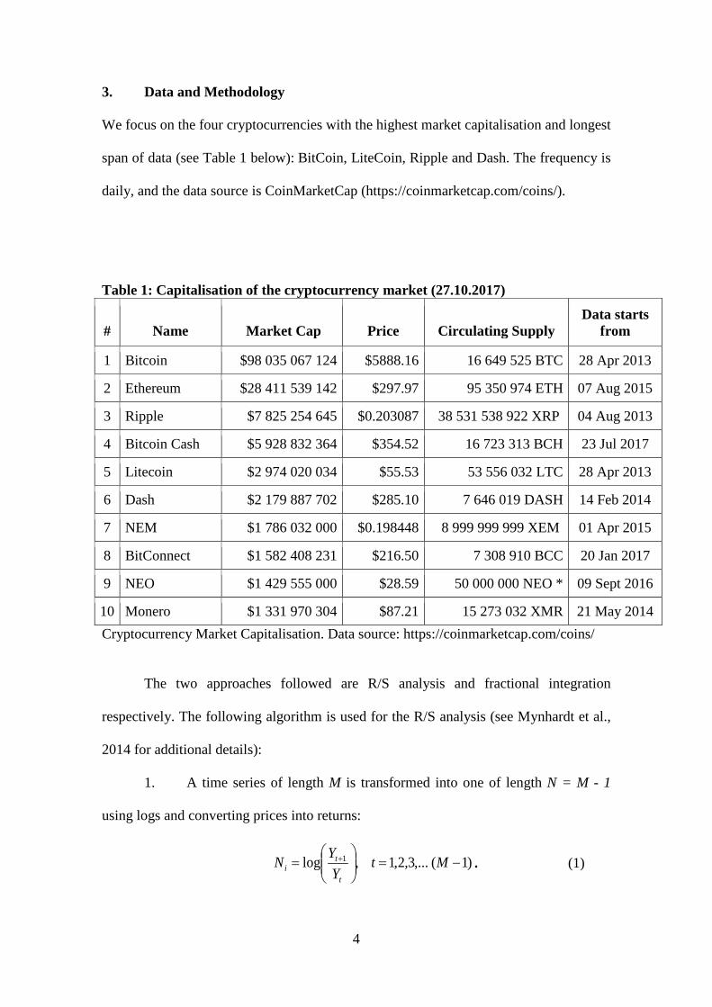
3. Data and Methodology

We focus on the four cryptocurrencies with the highest market capitalisation and longest

span of data (see Table 1 below): BitCoin, LiteCoin, Ripple and Dash. The frequency is

daily, and the data source is CoinMarketCap (https://coinmarketcap.com/coins/).

Table 1: Capitalisation of the cryptocurrency market (27.10.2017)

# Name Market Cap Price Circulating Supply Data starts

from

1 Bitcoin $98 035 067 124 $5888.16 16 649 525 BTC 28 Apr 2013

2 Ethereum $28 411 539 142 $297.97 95 350 974 ETH 07 Aug 2015

3 Ripple $7 825 254 645 $0.203087 38 531 538 922 XRP 04 Aug 2013

4 Bitcoin Cash $5 928 832 364 $354.52 16 723 313 BCH 23 Jul 2017

5 Litecoin $2 974 020 034 $55.53 53 556 032 LTC 28 Apr 2013

6 Dash $2 179 887 702 $285.10 7 646 019 DASH 14 Feb 2014

7 NEM $1 786 032 000 $0.198448 8 999 999 999 XEM 01 Apr 2015

8 BitConnect $1 582 408 231 $216.50 7 308 910 BCC 20 Jan 2017

9 NEO $1 429 555 000 $28.59 50 000 000 NEO * 09 Sept 2016

10 Monero $1 331 970 304 $87.21 15 273 032 XMR 21 May 2014 Cryptocurrency Market Capitalisation. Data source: https://coinmarketcap.com/coins/

The two approaches followed are R/S analysis and fractional integration

respectively. The following algorithm is used for the R/S analysis (see Mynhardt et al.,

2014 for additional details):

1. A time series of length M is transformed into one of length N = M - 1

using logs and converting prices into returns:

)1(,...3,2,1,log 1 −=

= + Mt

YYN

t

ti . (1)

5

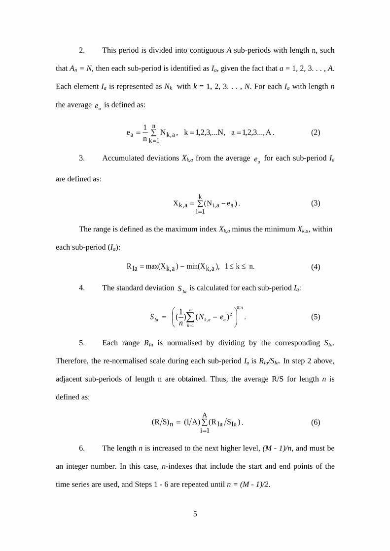
2. This period is divided into contiguous A sub-periods with length n, such

that An = N, then each sub-period is identified as Ia, given the fact that a = 1, 2, 3. . . , A.

Each element Ia is represented as Nk with k = 1, 2, 3. . . , N. For each Ia with length n

the average ae is defined as:

А...,3,2,1а,N,...3,2,1k,Nn1e

n

1ka,ka =∑ ==

=. (2)

3. Accumulated deviations Xk,a from the average ae for each sub-period Ia

are defined as:

)eN(X ak

1ia,ia,k −= ∑

=. (3)

The range is defined as the maximum index Xk,a minus the minimum Xk,a, within

each sub-period (Ia):

.nk1),Xmin()Xmax(R a,ka,kIa ≤≤−= (4)

4. The standard deviation IaS is calculated for each sub-period Ia:

5,0

1

2, )()1(

−= ∑

=

n

kaakIa eN

nS . (5)

5. Each range RIa is normalised by dividing by the corresponding SIa.

Therefore, the re-normalised scale during each sub-period Ia is RIa/SIa. In step 2 above,

adjacent sub-periods of length n are obtained. Thus, the average R/S for length n is

defined as:

∑=

=A

1iIaIan )SR()A1()SR( . (6)

6. The length n is increased to the next higher level, (M - 1)/n, and must be

an integer number. In this case, n-indexes that include the start and end points of the

time series are used, and Steps 1 - 6 are repeated until n = (M - 1)/2.

6

7. The least square method is used to estimate the equation log (R / S) = log

(c) + H*log (n). The slope of the regression line is an estimate of the Hurst exponent H.

(Hurst, 1951).

The Hurst exponent lies in the interval [0, 1]. On the basis of the H values three

categories can be identified: the series are anti-persistent, returns are negatively

correlated (0 ≤ H < 0.5); the series are random, returns are uncorrelated, there is no

memory in the series (H = 0.5); the series are persistent, returns are highly correlated,

there is memory in price dynamics (0.5 < H ≤ 1).

To analyse the dynamics of market persistence we use a sliding-window

approach. The procedure is the following: having obtained the first value of the Hurst

exponent (for example, for the date 01.04.2004 using data for the period from

01.01.2004 to 31.03.2004), each of the following ones is calculated by shifting forward

the “data window”, where the size of the shift depends on the number of observations

and a sufficient number of estimates is required to analyse the time-varying behaviour

of the Hurst exponent. For example, if the shift equals 10, the second value is calculated

for 10.04.2004 and characterises the market over the period 10.01.2004 till 09.04.2004,

and so on.

In addition we also employ I(d) techniques for the log prices series, both

parametric and semiparametric. Note that the differencing parameter d is related to the

Hurst exponential described above through the relationship H = d + 0.5. Also, R/S

analysis is used for the return series (the first differences of the log prices), while I(d)

models are estimated for the log prices themselves, in which case the relationship

becomes H = (d – 1) + 0.5 = d – 0.5. We consider processes of the form:

,...,2,1,)1( ==− tuxB ttd (7)

7

where B is the backshift operator (Bxt = xt-1); ut is an I(0) process (which may

incorporate weak autocorrelation of the AR(MA) form) and, xt are the errors of a

regression model of the form:

,...,2,1t;txt10ty =+β+β= (8)

where yt stands for the log price of each of the cryptocurrencies. Note that under the

Efficient Market Hypothesis the value of d in (7) should be equal to 1 and ut a white

noise process. As mentioned before, we use both parametric and semiparametric

methods, in each case assuming uncorrelated (white noise) and autocorrelated errors in

turn. More specifically, we use first the Whittle estimator of d in the frequency domain

(Dahlhaus, 1989; Robinson, 1994), and then the “local” Whittle estimator initially

proposed by Robinson (1995) and then further developed by Velasco (1999), Phillips

and Shimotsu (2005), Abadir et al. (2007) and others.

4. Empirical Results

The results of the R/S analysis for the return series of the four cryptocurrencies are

presented in Table 2.

Table 2: Results of the R/S analysis for the different crypto currencies, 2004-2017

Period Daily frequency

Bitcoin 0,59

LiteCoin 0,63

Ripple 0,64

Dash 0,60

As can be seen, the series do not follow a random walk, and are persistent,

which is inconsistent with market efficiency. The most efficient cryptocurrency is

Bitcoin, which is the oldest and most commonly used, as well as the most liquid.

8

The dynamic R/S analysis shows the evolution over time of persistence in the

cryptocurrency market (see Figure 1).

Figure 1: Results of the dynamic R/S analysis, (step=50, data window=300) Bitecoin

Litecoin

Ripple

Dash

0,400,450,500,550,600,650,70

2013

2013

2013

2013

2013

2014

2014

2014

2014

2014

2015

2015

2015

2015

2015

2016

2016

2016

2016

2016

2017

2017

2017

2017

0,400,450,500,550,600,650,70

2013

2013

2013

2013

2013

2014

2014

2014

2014

2014

2015

2015

2015

2015

2015

2016

2016

2016

2016

2016

2017

2017

2017

2017

0,35

0,45

0,55

0,65

0,75

2013

2013

2013

2013

2013

2014

2014

2014

2014

2014

2015

2015

2015

2015

2015

2016

2016

2016

2016

2016

2017

2017

2017

2017

9

As can be seen the degree of persistence varies over the time, and fluctuates

around its average. Time variation is particularly evident in the case of Litecoin, with

the exponent dropping significantly from 0.7 in 2013 to 0.50 in 2017. This represents

evidence in favour of the Adaptive Market Hypothesis (see Lo, 1991 for details) and

also of efficiency increasing over time. In the case of Litecoin the market was initially

rather inefficient, but after 2-3 years it became more liquid, and the number of

participants, trade volumes and efficiency all increased.

Next we estimate an I(d) model specified as:

,...,2,1t,ux)B1(,xty ttd

tt ==−+β+α= (9)

and test the null hypothesis:

,: oo ddH = (10)

in (9) for do-values equal to -1, -0.99, …. -0.01, 0, 0,01, … , 0.99 and 1 under different

modelling assumptions for the I(0) error term ut.

In Table 3 we assume that ut in (1) is a white noise process, and consider the

three cases of: i) no deterministic terms, ii) an intercept, and iii) an intercept with a

linear time trend. This table shows that the estimates are around 1 in all cases, which

implies non-stationary behaviour. A time trend is required in the cases of Bitcoin and

Dash, but not for the other two series, Litecoin and Ripple.

0,35

0,45

0,55

0,65

0,75

2013

2013

2013

2013

2013

2014

2014

2014

2014

2014

2015

2015

2015

2015

2015

2016

2016

2016

2016

2016

2017

2017

2017

2017

10

Table 3: Estimates of d and confidence bands for the case of no autocorrelation

Log series No terms An intercept A linear time trend

BITCOIN 0.992 (0.961, 1.040)

1.009 (0.983, 1.039)

1.009 (0.983, 1.039)

LITECOIN 1.005 (0.977, 1.038)

1.021 (0.994, 1.053)

1.021 (0.994, 1.053)

RIPPLE 1.028 (0.997, 1.064)

1.053 (1.023, 1.086)

1.053 (1.023, 1.087)

DASH 0.966 (0.933, 1.005)

0.985 (0.954, 1.022)

0.986 (0.954, 1.022)

Finally Table 4 (which focuses on the selected model for each series on the basis

of the deterministic terms) shows that the I(1) hypothesis cannot be rejected for three

series, namely Bitcoin, Litecoin and Dash. However, for Ripple it is rejected in favour

of d > 1. The implied values of the H exponent are slightly smaller than those reported

before: since H = d – 0.5, they are 0.51, 0.52, 0.53 and 0.48 respectively for Bitcoin,

Litecoin, Ripple and Dash, and the confidence intervals provide evidence of market

inefficiency only in the case of Ripple.

Table 4: Estimated coefficients in the selected models from Table 3

Log series d (95% band) Intercept Time trend

BITCOIN 1.009 (0.983, 1.039)

4.897 (114.15)

0.002 (1.79)

LITECOIN 1.021 (0.994, 1.053)

1.470 (21.60)

---

RIPPLE 1.053 (1.023, 1.086)

-5.313 (-66.89)

---

DASH 0.986 (0.954, 1.022)

-0.984 (-11.37)

0.005 (2.34)

Next we allow for autocorrelated disturbances, and for this purpose we use the

exponential spectral model of Bloomfield (see Bloomfield, 1973 for details). Table 5

displays the estimates of d for the three cases of no regressors, an intercept and a linear

time trend while Table 6 focuses on the selected models. As in the case of uncorrelated

11

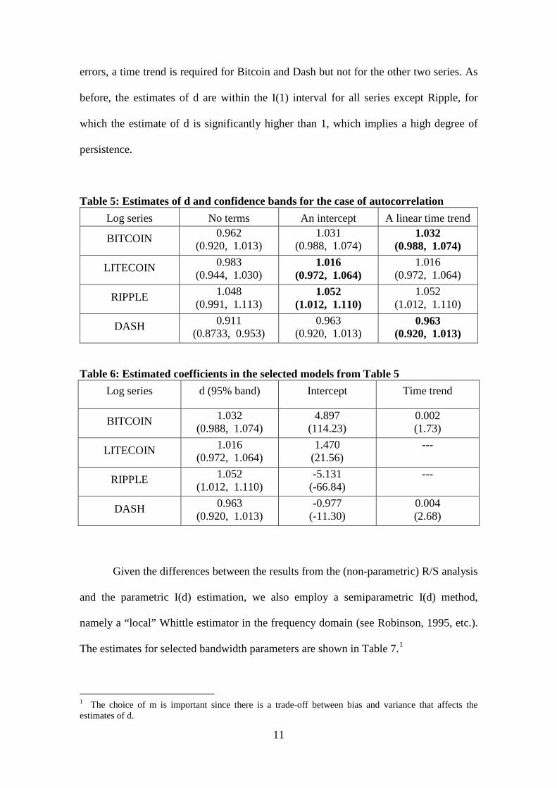
errors, a time trend is required for Bitcoin and Dash but not for the other two series. As

before, the estimates of d are within the I(1) interval for all series except Ripple, for

which the estimate of d is significantly higher than 1, which implies a high degree of

persistence.

Table 5: Estimates of d and confidence bands for the case of autocorrelation Log series No terms An intercept A linear time trend

BITCOIN 0.962 (0.920, 1.013)

1.031 (0.988, 1.074)

1.032 (0.988, 1.074)

LITECOIN 0.983 (0.944, 1.030)

1.016 (0.972, 1.064)

1.016 (0.972, 1.064)

RIPPLE 1.048 (0.991, 1.113)

1.052 (1.012, 1.110)

1.052 (1.012, 1.110)

DASH 0.911 (0.8733, 0.953)

0.963 (0.920, 1.013)

0.963 (0.920, 1.013)

Table 6: Estimated coefficients in the selected models from Table 5 Log series d (95% band) Intercept Time trend

BITCOIN 1.032 (0.988, 1.074)

4.897 (114.23)

0.002 (1.73)

LITECOIN 1.016 (0.972, 1.064)

1.470 (21.56)

---

RIPPLE 1.052 (1.012, 1.110)

-5.131 (-66.84)

---

DASH 0.963 (0.920, 1.013)

-0.977 (-11.30)

0.004 (2.68)

Given the differences between the results from the (non-parametric) R/S analysis

and the parametric I(d) estimation, we also employ a semiparametric I(d) method,

namely a “local” Whittle estimator in the frequency domain (see Robinson, 1995, etc.).

The estimates for selected bandwidth parameters are shown in Table 7.1

1 The choice of m is important since there is a trade-off between bias and variance that affects the estimates of d.

12

Table 7: Estimates of d based on a semiparametric Whittle method

Log series 30 32 34 36 38 40 42 44 46 38 50

BITCOIN 1.072 1.099 1.078 1.081 1.108 1.142 1.152 1.109 1.186 1.107 1.100

LITECOIN 1.123 1.173 1.096 1.125 1.141 1.174 1.122 1.101 1.101 1.103 1.076

RIPPLE 1.153 1.091 1.125 1.137 1.096 1.088 1.064 1.042 1.047 1.011 1.022

DASH 1.170 1.081 1.150 1.200 1.235 1.228 1.216 1.202 1.154 1.145 1.162

Lower I(1) 1.150 1.145 1.141 1.137 1.133 1.130 1.126 1.124 1.121 1.118 1.114

Upper I(1) 0.849 0.854 0.858 0.862 0.866 0.869 0.873 0.876 0.878 0.881 0.883

In bold those cases where the estimates of d are significantly higher than 1 at the 5% level.

The unit root hypothesis (i.e., d = 1) is rejected in many cases, especially for

Dash, but also for the other three series.

Figure 2 displays the estimates of d for all bandwidth parameters and Figure 3

focuses on values of m from 25 to 200.

Figure 2: Estimates of d based on semiparametric methods

Bitcoin

Litecoin

0,4

0,6

0,8

1

1,2

1,4

1,6

1 29 57 85 113 141 169 197 225 253 281 309 337 365 393 421 449 477 505 533 561 589 617 645 673 701 729 757 785

13

Ripple

Dash

Figure 3: Estimates of d based on semiparametric methods (with m = 25, …, 200)

Bitcoin

Litecoin

0,4

0,6

0,8

1

1,2

1,4

1,6

1 29 57 85 113 141 169 197 225 253 281 309 337 365 393 421 449 477 505 533 561 589 617 645 673 701 729 757 785

0,4

0,6

0,8

1

1,2

1,4

1,6

1 29 57 85 113 141 169 197 225 253 281 309 337 365 393 421 449 477 505 533 561 589 617 645 673 701 729 757 7850,4

0,6

0,8

1

1,2

1,4

1,6

1 29 57 85 113 141 169 197 225 253 281 309 337 365 393 421 449 477 505 533 561 589 617 645 673 701 729 757 785

0,7

0,8

0,9

1

1,1

1,2

1,3

1 6 11 16 21 26 31 36 41 46 51 56 61 66 71 76 81 86 91 96 101 106 111 116 121 126

14

Ripple

Dash

Depending on the bandwidth parameters the estimates of d are within the I(1)

interval or above 1. Therefore there is strong evidence that mean reversion does not

occur, which suggests market inefficiency.

5. Conclusions

This paper uses R/S analysis and fractional integration long-memory techniques to

examine the degree of persistence of the four main cryptocurrencies (BitCoin, LiteCoin,

Ripple and Dash) and its evolution over time. In brief, the evidence suggests that the

0,8

0,85

0,9

0,95

1

1,05

1,1

1,15

1,2

1 6 11 16 21 26 31 36 41 46 51 56 61 66 71 76 81 86 91 96 101 106 111 116 121 126

0,8

0,85

0,9

0,95

1

1,05

1,1

1,15

1,2

1 6 11 16 21 26 31 36 41 46 51 56 61 66 71 76 81 86 91 96 101 106 111 116 121 1260,7

0,8

0,9

1

1,1

1,2

1,3

1 6 11 16 21 26 31 36 41 46 51 56 61 66 71 76 81 86 91 96 101 106 111 116 121 126

15

cryptocurrency market is still inefficient, but is becoming less so. This is especially true

of the Litecoin market, where the Hurst exponent dropped considerably over time.

The results obtained using I(d) methods are less conclusive, since the estimated

values of d are higher than but not significantly different from 1 in a number of cases,

the main exception being Ripple for which the parametric estimate of d is significantly

higher than 1. The semiparametric I(d) results are very sensitive to the choice of the

bandwidth parameter, and market inefficiency is found in a number of cases.

Persistence implies predictability, and therefore represents evidence of market

inefficiency, suggesting that trend trading strategies can be used to generate abnormal

profits in the cryptocurrency market.

16

References

Abadir, K.M., Distaso, W. and Giraitis, L., (2007), Nonstationarity-extended local Whittle estimation, Journal of Econometrics 141, 1353-1384. Bariviera, Aurelio F., María José Basgall, Waldo Hasperué, Marcelo Naiouf, (2017), Some stylized facts of the Bitcoin market, In Physica A: Statistical Mechanics and its Applications, Volume 484, 2017, Pages 82-90. Bariviera, Aurelio F., (2017), The Inefficiency of Bitcoin Revisited: A Dynamic Approach. Economics Letters, Vol. 161, p. 1-4. Bartos, J., (2015), Does Bitcoin follow the hypothesis of efficient market?. International Journal of Economic Sciences, Vol. IV(2), pp. 10-23. Bloomfield, P., (1973), An exponential model in the spectrum of a scalar time series, Biometrika, 60, 217-226. Bouri, Elie, Georges Azzi, and Anne Haubo Dyhrberg (2016). On the Return-volatility Relationship in the Bitcoin Market Around the Price Crash of 2013. Economics Discussion Papers, No 2016-41, Kiel Institute for the World Economy. http://www.economics-ejournal.org/economics/discussionpapers/2016-41 Bouoiyour, Jamal and Selmi, Refk (2015). Bitcoin Price: Is it really that New Round of Volatility can be on way? MPRA Paper 65580, University Library of Munich, Germany. https://ideas.repec.org/p/pra/mprapa/65580.html Caporale, G.M., Gil-Alana, L.A., Plastun, A. and I. Makarenko, (2016), Long memory in the Ukrainian stock market and financial crises. Journal of Economics and Finance, 40, 2, 235-257. Caporale, Guglielmo Maria and Plastun, Oleksiy, (2017), The Day of the Week Effect in the Crypto Currency Market (October 20, 2017). Brunel University London, Department of Economics and Finance, Working Paper No. 17-19. Available at SSRN: https://ssrn.com/abstract=3056229 Carrick, J. (2016), Bitcoin as a Complement to Emerging Market Currencies, Emerging Markets Finance and Trade, vol. 52, 2016, pp. 2321-2334. Catania, Leopoldo and Grassi, Stefano, (2017), Modelling Crypto-Currencies Financial Time-Series (August 16, 2017). Available at SSRN: https://ssrn.com/abstract=3028486 Cheung, A., E. Roca and J.-J. Su, (2015), Crypto-Currency Bubbles: An Application of the Phillips-Shi-Yu (2013) Methodology on Mt. Gox Bitcoin Prices, Applied Economics, vol. 47, 2015, pp. 2348-2358. Dahlhaus, R., (1989), Efficient parameter estimation for self-similar process, Annals of Statistics, 17, 1749-1766.

17

Dwyer, G. P. (2014), The Economics of Bitcoin and Similar Private Digital Currencies, Journal of Financial Stability, vol. 17, 2014, pp. 81-91. ElBahrawy, Abeer; Alessandretti, Laura; Kandler, Anne; Pastor-Satorras, Romualdo; Baronchelli, (2017) Andrea Bitcoin ecology: Quantifying and modelling the long-term dynamics of the cryptocurrency market https://arxiv.org/abs/1705.05334 Fama, E (1970), Efficient Capital Markets: A Review of Theory and Empirical Evidence, Journal of Finance, No. 25, pp. 383-417. Greene, M.T. and Fielitz, B.D., (1977), Long-term dependence in common stock returns. Journal of Financial Economics 4, 339-349. Halaburda, Hanna and Gandal, Neil, (2014), Competition in the Cryptocurrency Market. NET Institute Working Paper No. 14-17. Available at SSRN: https://ssrn.com/abstract=2506463 or http://dx.doi.org/10.2139/ssrn.2506463 Hurst, H. (1951), Long-term storage of reservoirs, Transactions of the American Society of Civil Engineers, 116. Kurihara, Yutaka and Fukushima, Akio, (2017), The Market Efficiency of Bitcoin: A Weekly Anomaly Perspective Journal of Applied Finance & Banking, vol. 7, no. 3, 57-64. Lo, A.W., (1991), Long-term memory in stock market prices, Econometrica 59, 1279-1313. Mynhardt, R.H., Plastun A. and I. Makarenko, (2014), Behavior of financial markets efficiency during the financial market crisis: 2007 – 2009. Corporate Ownership and Control 11, 2, 473-488. Phillips, P.C. and Shimotsu, K., (2005), Exact local Whittle estimation of fractional integration. Annals of Statistics 33, 1890-1933. Robinson, P.M., (1994), Efficient tests of nonstationary hypotheses, Journal of the American Statistical Association 89, 1420-1437. Robinson, P.M., (1995), Gaussian semi-parametric estimation of long range dependence, Annals of Statistics 23, 1630-1661. Urquhart, A., (2016), The Inefficiency of Bitcoin, Economics Letters, vol. 148, 2016, 80-82. Velasco, C., (1999), Gaussian semiparametric estimation of nonstationary time series. Journal of Time Series Analysis. 20, 87-127.