17.874 Lecture NotesPart 4: Nonlinear Models

4. Non-Linear Models

4.1. Functional Form

We have discussed one important violation of the regression assumption { omitted vari-

ables. And, we have touched on problems of ine±ciency introduced by heteroskedasticity

and autocorrelation. This and the following subsections deal with violations of the regres-

sion assumptions (other than the omitted variables problem). The current section examines

corrections for non-linearity; the next section concerns discrete dependent variables. Follow-

ing that we will deal brie°y with weighting, heteroskedasticity, and autocorrelation. Time

permitting we will do a bit on Sensitivity.

We encounter two sorts of non-linearity in regression analysis. In some problems non-

linearity occurs among the X variables but it can be handled using a linear form of non-linear

functions of the X variables. In other problems non-linearity is inherent in the model: we

cannot \linearize" the relationship between Y and X. The ¯rst sort of problem is sometimes

called \intrinsically linear" and the second sort is \intrinsically non-linear."

Consider, ¯rst, situations where we can convert a non-linear model into a linear form.

In the Seats-Votes example, the basic model involved multiplicative and exponential param-

eters. We converted this into a linear form by taking logarithms. There are a wide range

of non-linearities that can arise; indeed, there are an in¯nite number of transformations of

variables that one might use. Typically we do not know the appropriate function and begin

with a linear relationship between Y and X as the approximation of the correct relationship.

We then stipulate possible non-linear relationships and implement transformations.

Common examples of non-linearities include:

Multiplicative models, where the independent variables enter the equation multiplicatively

rather than linearly (such models are linear in logarithms);

Polynomial regressions, where the independent variables are polynomials of a set of variables

1

(common in production function analysis in economics); and

Interactions, where some independent variables magnify the e®ects of other independent

variables (common in psychological research).

In each of these cases, we can use transformations of the independent variables to construct

a linear speci¯cation with with we can estimate all of the parameters of interest.

Qualitative Independent variables and interaction e®ects are the simplest sort of non-

linearity. They are simple to implement, but sometimes hard to interpret. Let's consider a

simple case. Ansolabehere and Iyengar (1996) conducted a series of laboratory experiments

involving approximately 3,000 subjects over 3 years. The experiments manipulated the

content of political advertisements, nested the manipulated advertisements in the commercial

breaks of videotapes of local newscasts, randomly assigned subjects to watch speci¯c tapes,

and then measured the political opinions and information of the subjects. These experiments

are reported in the book Going Negative.

On page 190, they report the following table.

E®ects of Party and Advertising Exponsure on Vote Preferences: General Election Experiments

Independent (1) (2) Variable Coe®. (SE) Coe®. (SE)

Constant .100 (.029) .102 (.029)

Advertising E®ects Sponsor .077 (.012) .023 (.034)

Sponsor*Same Party { .119 (.054) Sponsor*Opposite Party { .028 (.055)

Control Variables Party ID .182 (.022) .152 (.031) Past Vote .339 (.022) .341 (.022)

Past Turnout .115 (.030) .113 (.029) Gender .115 (.029) .114 (.030)

2

The dependent variable is +1 if the person stated an intention to vote Democratic after

viewing the tape, -1 if the person stated an intention to vote Republican, and 0 otherwise.

The variable Sponsor is the party of the candidate whose ad was shown; it equals +1 if the

ad was a Democratic ad, -1 if the ad was a Republican ad, and 0 if no political ad was shown

(control). Party ID is similarly coded using a trichotomy. Same Party was coded as +1 if

a person was a Democrat and saw a Democratic ad or a Republican and saw a Republican

ad. Opposite Party was coded as +1 if a person was a Democrat and saw a Republican ad

or a Republican and saw a Democratic ad.

In the ¯rst column, the \persuasion" e®ect is estimated as the coe±cient on the variable

Sponsor. The estimate is .077. The interpretation is that exposure to an ad from a candidate

increases support for that candidate by 7.7 percentage points.

The second column estimates interactions of the Sponsor variable with the Party ID vari-

able. What is the interpretation of the set of three variables Sponsor, Sponsor*Same Party

, and Sponsor*Opposite Party. The variables Same Party and Opposite Party encompass

all party identi¯ers. When these variables equal 0, the viewer is a non-partisan. So, the

coe±cient on Sponsor in the second column measures the e®ect of seeing an ad among inde-

pendent viewers. It increases support for the sponsor by only 2.3 percentage points. When

Same Party equals 1, the coe±cient on Sponsor is 11.9. This is not the e®ect of the ad

among people of the same party. It is the di®erence between the Independents and those of

the same party. To calculate the e®ect of the ad on people of the same party we must add

.119 to .023, yielding an e®ect of .142, or a 14.2 percentage point gain.

Interactions such as these allow us to estimate di®erent slopes for di®erent groups, changes

in trends, and other discrete changes in functional forms.

Another class of non-linear speci¯cations takes the form of Polynomials. Many theories

of behavior begin with a conjecture of an inherently non-linear function. For instance, a

¯rm's production function is thought to exhibit decreasing marginal returns on investments,

capital or labor. Also, risk aversion implies a concave utility function.

3

Barefoot empiricism sometimes leads us to non-linearity, too. Examination of data, either

a scatter plot or a residual plot, may reveal a non-linear relationship, between Y and X .

While we do not know what the right functional form is, we can capture the relationship in

the data by including additional variables that are powers of X, such as X1=2 , X 2 , X3 , as

well as X . In other words, to capture the non-linear relationship, y = g(x), we approximate

the unknown function , g(x), using a polynomial of the values of x.

One note of caution. Including powers of independent variables often leads to collinearity

among the righthand side variables. Deviating the independent variables from their means

before transforming them.

Example: Candidate Convergence in Congressional Elections.

An important debate in the study of congressional elections concerns how well candi-

dates represent their districts. Two conjectures concern the extent to which candidates

re°ect their districts. First, are candidates responsive to districts? Are candidates in more

liberal districts more liberal? Second, does competitiveness lead to closer representation of

district preferences? In highly competitive districts, are the candidates more \converged"?

Huntington posits greater divergence of candidates in competitive areas { a sort of clash of

ideas.

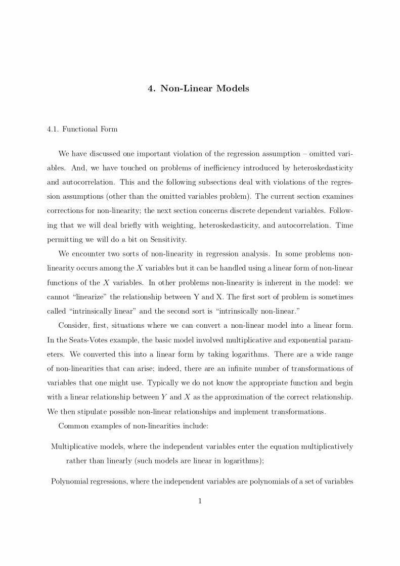
Ansolabehere, Snyder, and Stewart (2001) analyze data from a survey of congressional

candidates on their positions on a range of issues during the 1996 election. There are 292

districts in which both of the competing candidates ¯lled out the survey. The authors con-

structed a measure of candidate ideology from these surveys, and then examine the midpoint

between the two candidates (the cutpoint at which a voter would be indi®erent between the

candidates) and the ideological gap between the candidates (the degree of convergence). To

measure electoral competitiveness the authors used the average share of vote won by the

Democratic candidate in the prior two presidential elections (1988 and 1992).

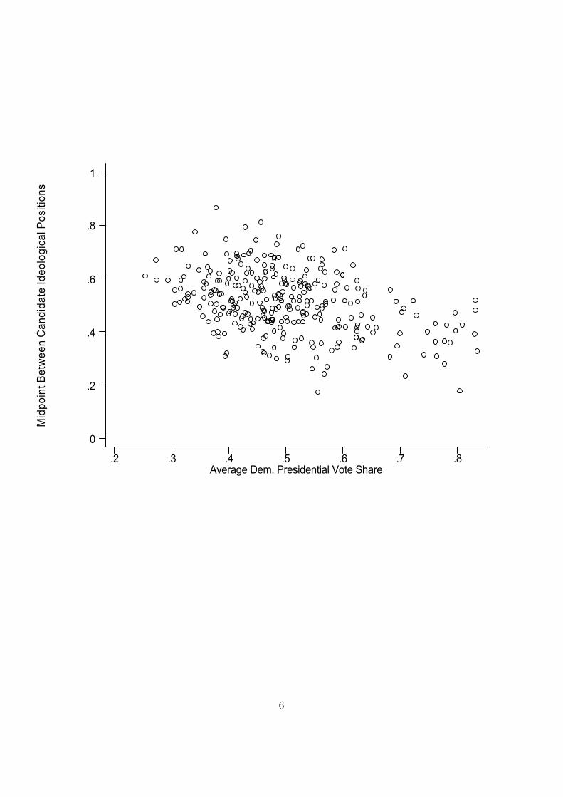
The Figures show the relationship between Democratic Presidential Vote share and,

respectively, candidate midpoints and the ideological gap between competing candidates.

4

There is clear evidence of a non-linear relationship explaining the gap between the candi-

dates

The table presents a series of regressions in which the Midpoint and the Gap are predicted

using quadratic functions of the Democratic Presidential Vote plus an indicator of Open

Seats, which tend to be highly competitive. We consider, separately, a speci¯cation using

the value of the independent variable and its square and a speci¯cation using the value

of the independent variable deviated from its mean and its square. The last column uses

the absolute value of the deviation of the presidential vote from .5 as an alternative to the

quadratic.

E®ects of District Partisanship on Candidate PositioningN = 292

Dependent Variable Midpoint Gap

Independent (1) (2) (3) (4) (5) Variable Coe®.(SE) Coe®.(SE) Coe®. (SE) Coe®. (SE) Coe®. (SE)

Democratic Presidential -.158 (.369) | -2.657 (.555) | | Vote

Democratic Presidential -.219 (.336) | +2.565 (.506) | | Vote Squared

Dem. Pres. Vote | -.377 (.061) | -.092 (.092) | Mean Deviated

Dem. Pres. Vote | -.219 (.336) | +2.565 (.506) | Mean Dev. Squared

Absolute Value of Dem. Pres. | | | | .764 (.128) Vote, Mean Dev.

Open Seat .007 (.027) .007 (.027) -.024 (.040) -.024 (.040) -.017 (.039) Constant .649 (.098) .515 (.008) 1.127 (.147) .440 (.012) .406 (.015) R2 .156 .156 .089 .089 .110 pMSE .109 .109 .164 .164 .162

F (p-value) 18.0 (.00) 18.0 (.00) 9.59 (.00) 9.59 (.00) 12.46 (.00)

5

Mid

po

int

Be

twe

en

Ca

nd

ida

te I

de

olo

gic

al P

osit

ion

s

0

.2

.4

.6

.8

1

.2 .3 .4 .5 .6 .7 .8 Average Dem. Presidential Vote Share

6

Ide

olo

gic

al

Ga

p B

etw

ee

n C

an

did

ate

s

0

.2

.4

.6

.8

1

.2 .3 .4 .5 .6 .7 .8 Average Dem. Presidential Vote Share

7

Consider, ¯rst, the regressions explaining the midpoint (columns 1 and 2). We expect

that the more liberal the districts are the more to the leftward the candidates will tend. The

ideology measure is oriented such that higher values are more conservative positions. Figure

1 shows a strong relationship consistent with the argument.

Column (1) presents the estimates when we naively include Presidential vote and Pres-

idential vote squared. This is a good example of what collinearity looks like. The F-test

shows that the regression is \signi¯cant" { i.e., not all of the coe±cients are 0. But, neither

the coe±cient on Presidential Vote or Presidential Vote Squared are sign¯cant. Tell-tale

collinearity. A trick for breaking the collinearity in this case is by deviating X from its mean.

Doing so, we ¯nd a signi¯cant e®ect on the linear coe±cient, but the quadratic coe±cient

doesn't change. There is only really one free coe±cient here, and it looks to be linear.

The coe±cients in a polynomial regression measure the partial derivatives of the un-

known function evaluated at the mean of X. Taylor's approximation leads us immediately

to this interpretation of the coe±cients for polynomial models. Recall from Calculus that

Taylor's Theorem allows us to express any function as a sum of derivatives of that function

evaluated at a speci¯c point. We may choose any degree of approximation to the function

by selecting a speci¯c degree of approximation. A ¯rst-order approximation uses the ¯rst

derivatives; a second order approximation uses the second derivatives; and so on. A second

order approximation of an unknown fuction, then, may be expressed as:

1 yi ¼ ® + ¯0 xi + x

2

where " # @f (x)

g0 = @x

0H ;0 ixi

x=x0 " # @2f (x)

H0 = 0@x@x x=x0

1 ® = f (x0) ¡ g 0 +0x0

0H0 0x0x 2

¯ = g0 ¡ H0x0:

8

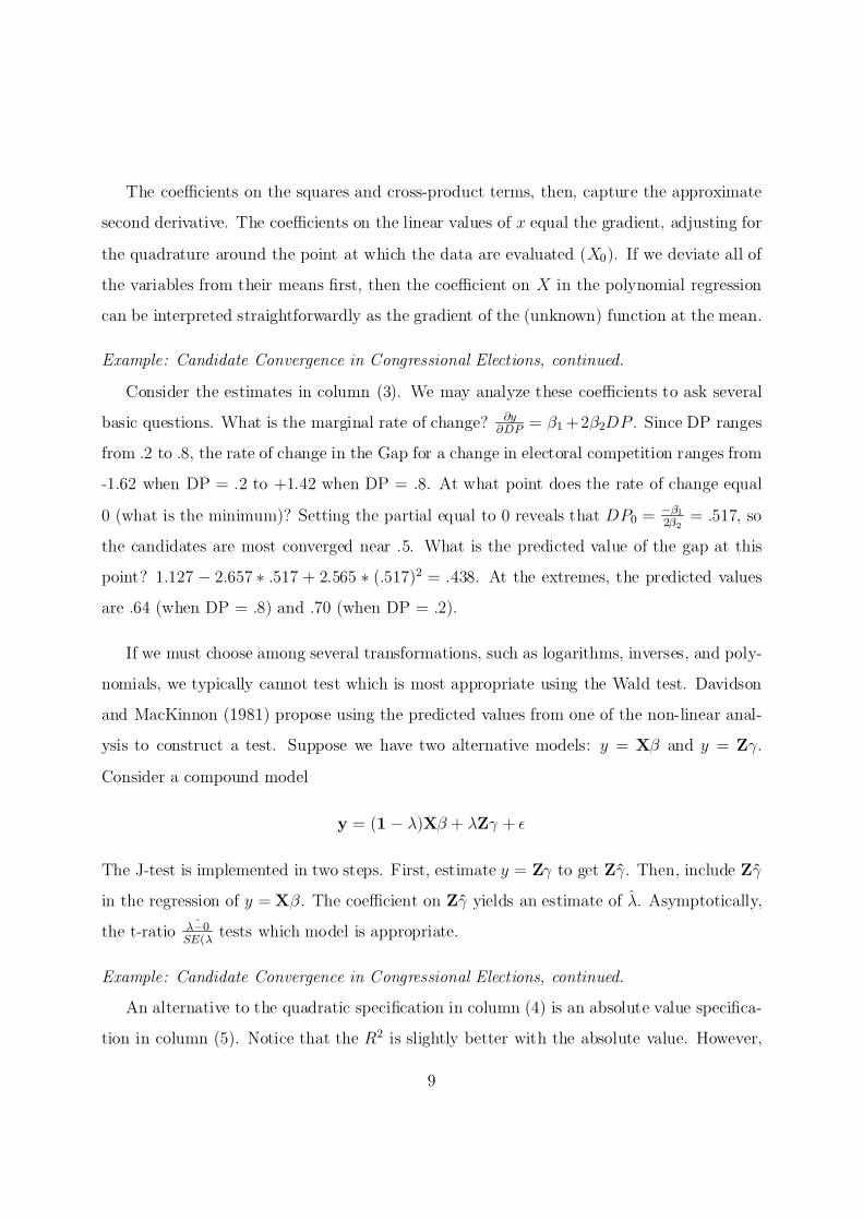
The coe±cients on the squares and cross-product terms, then, capture the approximate

second derivative. The coe±cients on the linear values of x equal the gradient, adjusting for

the quadrature around the point at which the data are evaluated (X0 ). If we deviate all of

the variables from their means ¯rst, then the coe±cient on X in the polynomial regression

can be interpreted straightforwardly as the gradient of the (unknown) function at the mean.

Example: Candidate Convergence in Congressional Elections, continued.

Consider the estimates in column (3). We may analyze these coe±cients to ask several @ybasic questions. What is the marginal rate of change? @DP = ¯1 +2¯2DP . Since DP ranges

from .2 to .8, the rate of change in the Gap for a change in electoral competition ranges from

-1.62 when DP = .2 to +1.42 when DP = .8. At what point does the rate of change equal

0 (what is the minimum)? Setting the partial equal to 0 reveals that DP0 = ¡¯ 1 = :517, so 2¯ 2

the candidates are most converged near .5. What is the predicted value of the gap at this

point? 1:127 ¡ 2:657 ¤ :517 + 2:565 ¤ (:517)2 = :438. At the extremes, the predicted values

are .64 (when DP = .8) and .70 (when DP = .2).

If we must choose among several transformations, such as logarithms, inverses, and poly-

nomials, we typically cannot test which is most appropriate using the Wald test. Davidson

and MacKinnon (1981) propose using the predicted values from one of the non-linear anal-

ysis to construct a test. Suppose we have two alternative models: y = X¯ and y = Z°.

Consider a compound model

y = (1 ¡ ¸)X¯ + ¸Z° + ²

°. Then, include Z^The J-test is implemented in two steps. First, estimate y = Z° to get Z^ °

^in the regression of y = X¯. The coe±cient on Z°̂ yields an estimate of ¸. Asymptotically, ^

the t-ratio ¸¡0 tests which model is appropriate. SE(¸

Example: Candidate Convergence in Congressional Elections, continued.

An alternative to the quadratic speci¯cation in column (4) is an absolute value speci¯ca-

tion in column (5). Notice that the R2 is slightly better with the absolute value. However,

9

owing to collinearity, it is hard to test which model is more appropriate. I ¯rst regress on

Gap on DP and DP 2 and Open and generated predicted values, call these GapHat. I then

regress Gap on ZG and jDP ¡ :5j and Open. The coe±cient on jDP ¡ :5j is 1.12 with a

standard error of .40, so the t-ratio is above the critical value for statistical signi¯cance.

The coe±cient on ZG equals -.55 with a standard error of .58. The estimated ¸ is not

signi¯cantly di®erent from 0; hence, we favor the absolute value speci¯cation.

10

4.2 Qualitative Dependent Variables.

4.2.1. Models.

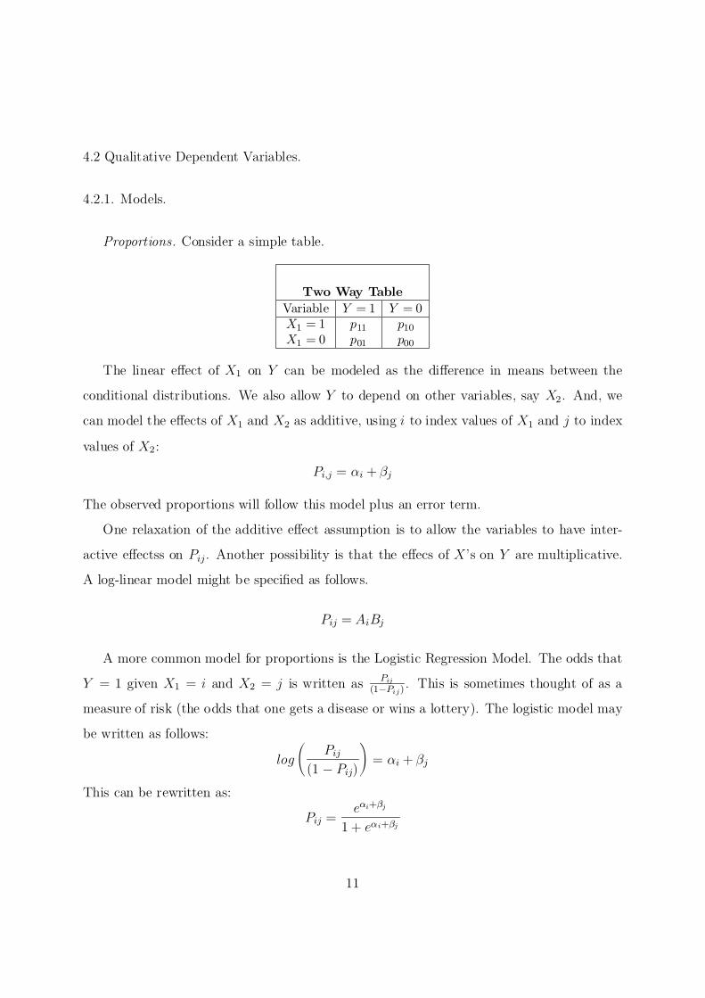
Proportions. Consider a simple table.

Two Way TableVariable Y = 1 Y = 0 X1 = 1 p11 p10 X1 = 0 p01 p00

The linear e®ect of X1 on Y can be modeled as the di®erence in means between the

conditional distributions. We also allow Y to depend on other variables, say X2 . And, we

can model the e®ects of X1 and X2 as additive, using i to index values of X1 and j to index

values of X2 :

Pi;j = ®i + ̄ j

The observed proportions will follow this model plus an error term.

One relaxation of the additive e®ect assumption is to allow the variables to have inter-

active e®ectss on Pij . Another possibility is that the e®ecs of X's on Y are multiplicative.

A log-linear model might b e speci¯ed as follows.

Pij = Ai Bj

A more common model for proportions is the Logistic Regression Model. The odds that PijY = 1 given X1 = i and X2 = j is written as (1¡Pij )

. This is sometimes thought of as a

measure of risk (the odds that one gets a disease or wins a lottery). The logistic model may

be written as follows: Ã ! Pij

log = ®i + ̄ j(1 ¡ Pij)

This can be rewritten as: ®i+¯ je

Pij = 1 + e®i+¯ j

11

The table proportions themselves may be thought of as the aggregation of n individual

observations on Y . The logistic regression, then, approximates an individual level Logit

regression in which the dependent variable takes values 1 and 0, and the independent vari-

ables may take many values. Above we assume that they take just 2 values each. The logit

function is called a \link" function, as it tells us how the additive e®ects are related to the

dependent variables.

Latent Variables. A second way that qualitative dependent variables arise in social sci-

ences is when there is a choice or outcome variable that depends on an underlying \latent"

variable, assumed continuous. Common examples include voting, random utility models of

consumer behavior, and cost-bene¯t calculations. The text discusses random utility models

and cost bene¯t calculations. Let's consider voting models here.

When a legislator or individual votes, they make a decision between two alternatives, each

of which is characterized by attributes. In spatial theories of voting, person i choose between

two alternatives j and k. The person has a most prefered outcome, call it µi , and the two

alternatives (parties, candidates, or proposals) represent points on the line, Xj and Xk. The

voter's preferences are represented as distances from the ideal point: ui (Xj ; µi) = ¡(Xj ¡ µi)2 .

There may be some uncertainty about the exact distance, so ui(Xj ; µi ) = ¡(Xj ¡ µi )2 + ²j .

The voter chooses the alternative closer to his or her ideal point. That is, voter i chooses j

over k if:

[¡(Xj ¡ µi )2] ¡ [¡(Xk ¡ µi )

2] + ² j ¡ ² k > 0

The latent variable, Y ¤, is a linear function of the set of independent variables, X. That

is,

¤ y = X¯ + ²:

However, we only observe qualitative outcomes. For example, y¤ might represent how in-

tensely someone supports or opposes a proposal, but we only observe whether they vote for

the proposal or not. That is, we observe: y = 1 if y¤ > c and 0 otherwise.

12

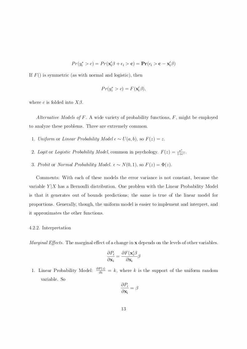
i i Pr(y > c) = Pr(x > c) = Pr(² > c ¡ x 0i

If F () is symmetric (as with normal and logistic), then

0

i¤ i ¯ + ² ¯)

P r(y > c) = F (x 0i¤ i ¯);

where c is folded into X¯.

Alternative Models of F . A wide variety of probability functions, F , might be employed

to analyze these problems. Three are extremely common.

1. Uniform or Linear Probability Model ² » U(a; b), so F (z) = z.

ze2. Logit or Logistic Probability Model, common in psychology. F (z) = 1+ez .

3. Probit or Normal Probability Model. ² » N(0; 1), so F (z) = ©(z).

Comments: With each of these models the error variance is not constant, because the

variable Y jX has a Bernoulli distribution. One problem with the Linear Probability Model

is that it generates out of bounds predictions; the same is true of the linear model for

proportions. Generally, though, the uniform model is easier to implement and interpret, and

it approximates the other functions.

4.2.2. Interpretation

Marginal E®ects. The marginal e®ect of a change in x depends on the levels of other variables.

@Pi @F (x0i¯ = ¯

@xi @xi

1. Linear Probability Model: @F(z) @z = k, where k is the support of the uniform random

variable. So @Pi

= ¯ @xi

13

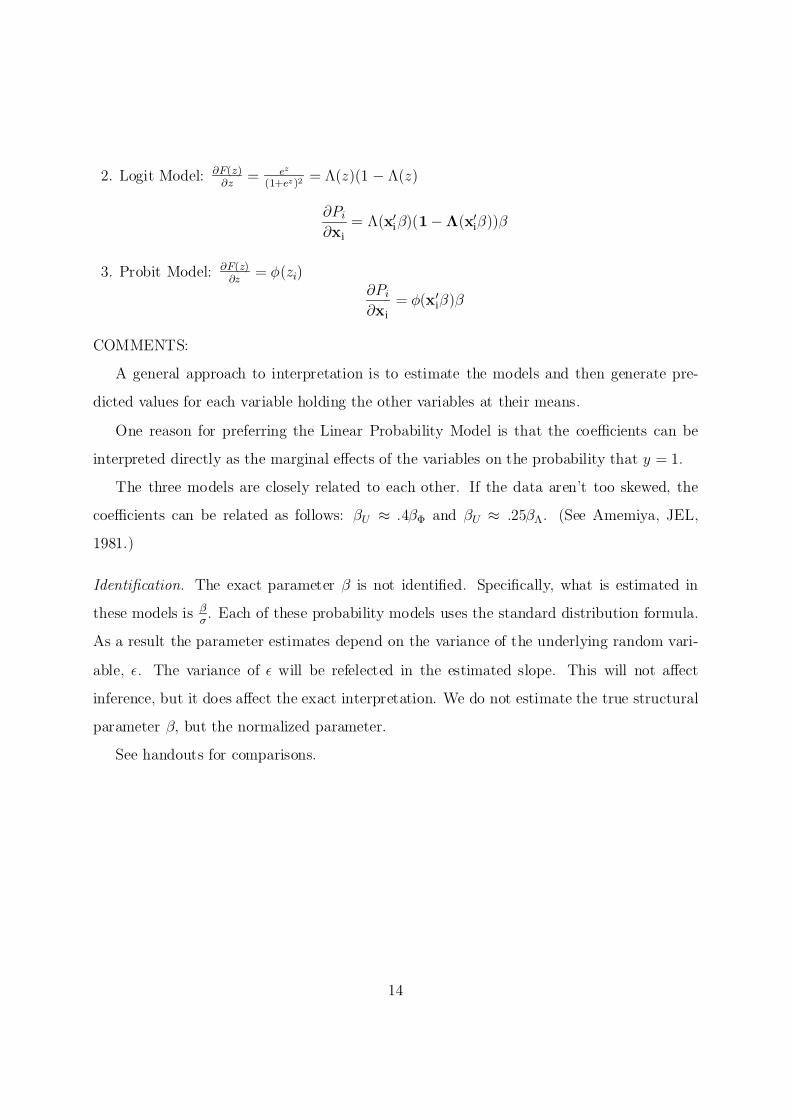
ze2. Logit Model: @F(z) = (1+ez )2 = ¤(z)(1 ¡ ¤(z)

@z

@Pi = ¤(x

@xi

@F(z) = Á(zi)3. Probit Model: @z

@Pi

0

i¯)(1 ¡ ¤(x ¯))¯0

i

= Á(x0i¯)¯ @xi

COMMENTS:

A general approach to interpretation is to estimate the models and then generate pre-

dicted values for each variable holding the other variables at their means.

One reason for preferring the Linear Probability Model is that the coe±cients can be

interpreted directly as the marginal e®ects of the variables on the probability that y = 1.

The three models are closely related to each other. If the data aren't too skewed, the

coe±cients can be related as follows: ¯ U ¼ :4¯ © and ¯ U ¼ :25¯ ¤ . (See Amemiya, JEL,

1981.)

Identi¯cation. The exact parameter ¯ is not identi¯ed. Speci¯cally, what is estimated in ¯ these models is ¾. Each of these probability models uses the standard distribution formula.

As a result the parameter estimates depend on the variance of the underlying random vari-

able, ². The variance of ² will be refelected in the estimated slope. This will not a®ect

inference, but it does a®ect the exact interpretation. We do not estimate the true structural

parameter ¯, but the normalized parameter.

See handouts for comparisons.

14

4.3. Estimation

The probit and logit models are usually estimated using the method of Maximum Like-

lihood. The maximization methods do not yield closed-form solutions to the parameters of

interest. So, we must approximate an exact solution using algorithms. I will review these

brie°y here to give you a sense of exactly what is estimated.

4.3.1. Likelihood Function

To construct the likelihood function, we consider, ¯rst, the distribution of the random

variable Yijxi. In the problem at hand, Yi is a Bernoulli random variable. Denote the

0observed values of Y as yi = 1 or 0, and note that pi = F (xi¯). We can write the density

for a given i as

0P (Yi = 1) = pyi (1 ¡ pi )1¡yi = F (x ¯)yi (1 ¡ F(x 0 ¯)(1¡yi):i i i

We observe n observations, i = 1; :::n. Assuming that the observations are independent of

each other, the joint density, or likelihood, is:

0 0L = ¦n F (x ¯)yi(1 ¡ F(x ¯))(1¡yi) i=1 i i

The logarithm of the likelihood function is

n X ln(L) =

i=1 yi ln(F (x 0 i¯)) + (1 ¡ yi)ln(1 ¡ F(x 0 i¯)) (1)

X X =

i2(y=1)

ln(F (x 0 i¯)) + i2(y=0)

ln(1 ¡ F(x 0 i¯)) (2)

To fully specify the likelihood function, substitute the particular formula for F , e.g., F (z) = ze or F (z) = ©(z).(1+ez)

15

4.3.2. Maximum Likelihood Estimation

Maximum likelihood estimates are values of ¯ and ¾ such that ln(L) is maximized. The

gradient of the log-likelihood function with respect to ¯ is:

0

i (1 ¡ yi)f (x 0i(1 ¡ F(x ¯))0

i

n@ln(L) X yi f(x ¯) ¯) (3)

(F (xxi ¡0

ixi=

¯ ¯)i=1 n 0

if(x¯)X 0 iF (x

(yi ¡ F (x

In the case of the Logit model, fi = ¤i (1 ¡ ¤i), so the ¯rst order conditions are:

n@ln(L) X = (yi ¡ ¤(xi

0¯̂))xi = 0 ¯

0

i

i=1

In the case of the Probit model

¯))xi (4) =0

i¯)(1 ¡ F(x¯))i=1

¯̂))Á(x 0i¯̂)n

0

i

0

i 0

i

(yi ¡ ©(x

©(x ¯̂)(1 ¡ ©(x

@ln(L) X xi=

¯̂))¯ i=1

^For neither one of these can we ¯nd an explicit solution for ¯.

A solution is found using algorithms that calculate successive approximations using Tay-

lor's Theorem. From Taylor's Theorem, a ¯rst-order approximation to the ¯rst order condi-

tion is: @ln(L) ^¼ g(¯0) + H(¯0)(¯ ¡ ¯0) = 0;¯

where ¯0 is the value at which we approximate the function, g(¯0 ) is the gradient at this

point, H(¯0) is the Hessian evaluated at this point. We will treat ¯0 as an initial guess,

usually a vector of 0's. We can rewrite this formula to have the following \updating formua,"

where ¯1 is our \updated guess":

¯1 = ¯0 ¡ H (¯0 )¡1g(¯0)

The updating formula can be used iteratively to arrive at a value of bt, for the t-th iteration.

The program will converge to a solution when bt+1 ¼ bt, to a chosen degree of approximation.

In maximum likelihood estimation the convergence criterion used is the change in the log-

likelihood between successive iterations. The value of bt is substituted into the log-likelihood

16

formula to calculate this value. When the percentage change in the log-likelihood is very

small, the program \converges." See the handout.

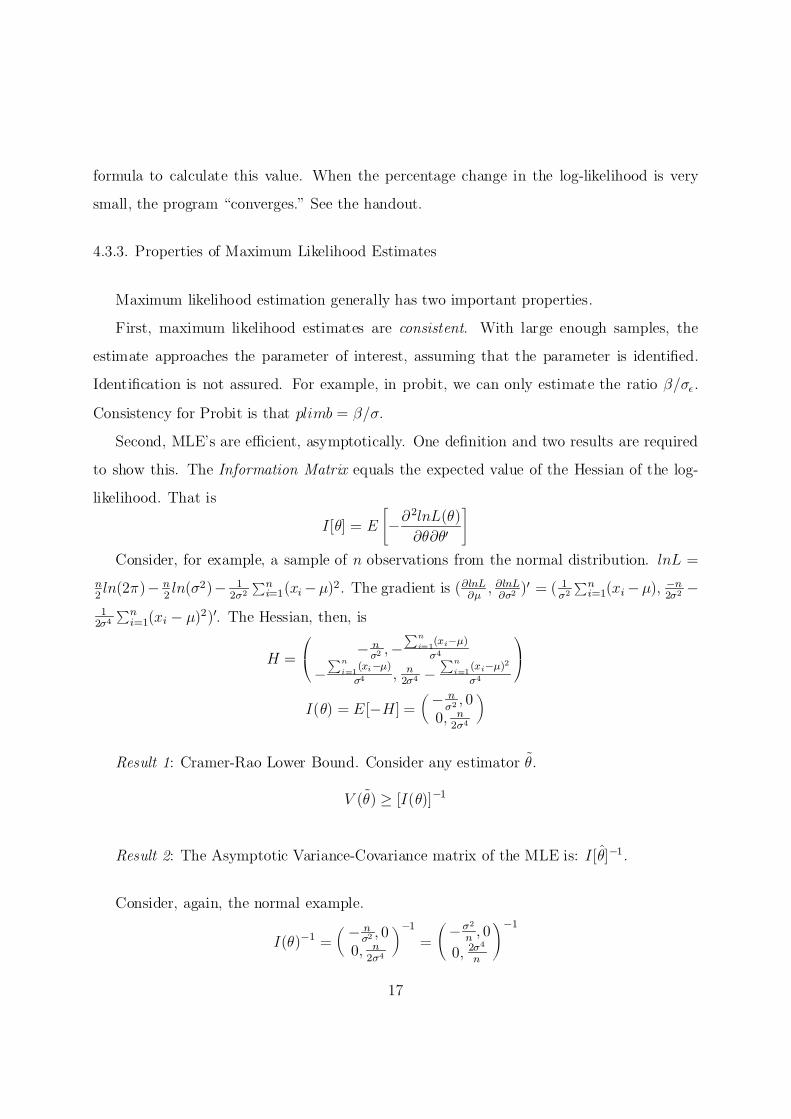
4.3.3. Properties of Maximum Likelihood Estimates

Maximum likelihood estimation generally has two important properties.

First, maximum likelihood estimates are consistent. With large enough samples, the

estimate approaches the parameter of interest, assuming that the parameter is identi¯ed.

Identi¯cation is not assured. For example, in probit, we can only estimate the ratio ¯=¾² .

Consistency for Probit is that plimb = ¯=¾.

Second, MLE's are e±cient, asymptotically. One de¯nition and two results are required

to show this. The Information Matrix equals the expected value of the Hessian of the log-

likelihood. That is " # @2lnL(µ)

I[µ] = E ¡ @µ@µ0

Consider, for example, a sample of n observations from the normal distribution. lnL = P Pn n 1 nln(2¼) ¡ ln(¾2 ) ¡ i=1 (xi ¡ ¹)2 . The gradient is (@lnL @¹ ;

@lnL )0 = ( 1 in =1(xi ¡ ¹); ¡n ¡

2 2 2¾2 @¾2 ¾2 2¾2 P1 n i=1(xi ¡ ¹)2 )0. The Hessian, then, is 2¾4 P 0 n 1

(xi¡¹)i=1¡ ¾n 2 ; ¡@ P P AH = ¾4

n n(xi ¡¹) (xi¡¹)

2

¡ i=1 n ¡ i=1 ¾4 ; 2¾4 ¾4 ¶¡

¾n 2 ; 0 I(µ) = E [¡H] =

µ

n0; 2¾4

~ Result 1: Cramer-Rao Lower Bound. Consider any estimator µ.

~ V (µ) ¸ [I(µ)]¡1

Result 2: The Asymptotic Variance-Covariance matrix of the MLE is: I[µ̂]¡1 .

Consider, again, the normal example. µ ¡ ¾2 ; 0

¶¡1 à ¡ ¾2 ; 0 ! ¡1n

nI(µ)¡1 =0; 2¾4

=0; 2¾

4n n

17

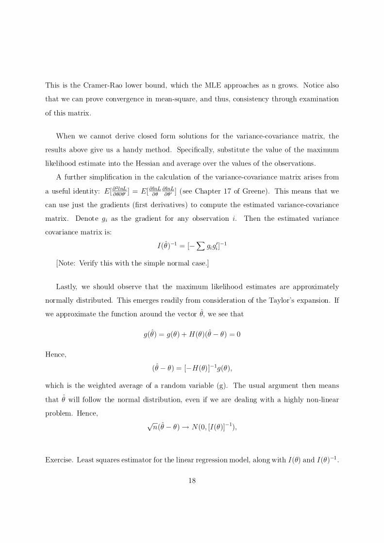
This is the Cramer-Rao lower bound, which the MLE approaches as n grows. Notice also

that we can prove convergence in mean-square, and thus, consistency through examination

of this matrix.

When we cannot derive closed form solutions for the variance-covariance matrix, the

results above give us a handy method. Speci¯cally, substitute the value of the maximum

likelihood estimate into the Hessian and average over the values of the observations.

A further simpli¯cation in the calculation of the variance-covariance matrix arises from

a useful identity: @2lnL ] = E[ @lnL @lnL ] (see Chapter 17 of Greene). This means that we E[ @µ@µ0 @µ @µ0

can use just the gradients (¯rst derivatives) to compute the estimated variance-covariance

matrix. Denote gi as the gradient for any observation i. Then the estimated variance

covariance matrix is:

^ X

0I(µ)¡1 = [¡ gigi]¡1

[Note: Verify this with the simple normal case.]

Lastly, we should observe that the maximum likelihood estimates are approximately

normally distributed. This emerges readily from consideration of the Taylor's expansion. If

^we approximate the function around the vector µ, we see that

^ ^ g(µ) = g(µ) + H(µ)(µ ¡ µ) = 0

Hence,

^(µ ¡ µ) = [¡H(µ)]¡1g(µ);

which is the weighted average of a random variable (g). The usual argument then means

^ that µ will follow the normal distribution, even if we are dealing with a highly non-linear

problem. Hence, pn(µ ̂ ¡ µ) ! N (0; [I(µ)]¡1);

Exercise. Least squares estimator for the linear regression model, along with I(µ) and I(µ)¡1 .

18

4.4. Inference

4.4.1. Con¯dence Intervals

As with the regression model we wish to construct con¯dence intervals and conduct

statistical tests on single coe±cients. While the values of the coe±cients may be di±cult to

interpret immediately, statistical testing is relatively straightforward.

To conduct inferences about single parameters, consider the marginal distribution of

a single parameter estimate. Because of normality, we know that the distribution of any

parameter estimate, say bk , will have mean ̄ k and variance equal to the kth diagonal element

of I(µ)¡1 , akk . Hence,

Pr(jbk ¡ ¯ j > z®=2 pakk ) < ®k

Therefore, a 95 percent con¯dence interval for ¯k is

bk § z1:96pakk

Examples: see handouts.

4.4.1. Likelihood Ratio Tests

As with our earlier discussion of inference, we can drawm mistaken conclusions { putting

too much or too little con¯dence in an inference { if we use the procedure for a single

coe±cient across many coe±cients. The analogue of the Wald-test in the likelihood based

models is the likelihood ratio test.

Consider two models. For simplicity assume that one of the models is a proper subset

of the others { that is, the variables included in one of the models encompasses that in

another model. The implicit hypothesis is that the subset of excluded variables from the

more parsimonious model all have coe±cients equal to 0. This amounts to a constraint

on the maximum likelihood estimates. The unrestricted model will necessarily have higher

likelihood. Is the di®erence in the likelihoods signi¯cant?

19

The likelihood ratio is calculated by evaluating the likelihood functions at the vector of

co±cients in the two models. The ratio of the likelihood statistics is:

^ ^ L(µR) ¸ = :

^L(µU )

This ratio is always less than 1. If it is much less than 1 then there is some evidence against

the hypothesis.

The relevant probability distribution can be derived readily for the log of of the likelihood

statistic.

^ ^ ¡2ln¸ = ¡2(ln(L(µR)) ¡ ln(L(µU )) » Â2 J

where J is the number of parameters restricted by the hypothesis.

Why does this follow the Â2? This is readily evident for the normal case. The log of the

normal function yields the sum of squares. So the log of the likelihood is the di®erence in

the sums of squares { i.e., the di®erence between two estimated variances.

It should be noted that this is the same information as used in the Wald test { the loss of

¯t. The Wald test di®ers primarily in that it normalizes by the ¯t of the unrestricted model.

It can be shown that asymptotically, Wald and Likelihood ratio statistics are the same.

20