18-753: information theory and coding lecture 1
TRANSCRIPT

18-753: Information Theory and CodingLecture 1: Introduction and Probability ReviewNotes build on those of Bobak Nazer at BU
Prof. Pulkit Grover
CMU
January 14, 2020

Syllabus
Syllabus: is here.

Bits and Information Theory
• More often than not, today’s information is measured in bits.
• Why?
• Is it ok to represent signals as different as audio and video in thesame currency, bits?
• Also, why do I communicate over long distances with the exact samecurrency?
Bits and Information Theory
• More often than not, today’s information is measured in bits.
• Why?
• Is it ok to represent signals as different as audio and video in thesame currency, bits?
• Also, why do I communicate over long distances with the exact samecurrency?

Bits and Information Theory
• More often than not, today’s information is measured in bits.
• Why?
• Is it ok to represent signals as different as audio and video in thesame currency, bits?
• Also, why do I communicate over long distances with the exact samecurrency?

Bits and Information Theory
• More often than not, today’s information is measured in bits.
• Why?
• Is it ok to represent signals as different as audio and video in thesame currency, bits?
• Also, why do I communicate over long distances with the exact samecurrency?

Video
• Video signals are made up of colors thatvary in space and time.
• Even if we are happy with pixels on ascreen how do we know that all thesecolors are optimally described by bits?

Audio
• Audio signals can be thought ofas an amplitude that variescontinuously with time.
• How can we optimally represent acontinuous signal in somethingdiscrete like bits?
0 0.1 0.2 0.3 0.4 0.5 0.6 0.7 0.8 0.9 1−10
−5
0
5
10
15
Just a Single Bit
• These (and many other) signals can all be optimally represented bybits.
• Information theory explains why and how.
• For now, let’s say we have a single bit that we really want tocommunicate to our friend. Let’s say it represents whether or not itis going to snow tonight.

Communication over Noisy Channels
• Let’s say we have to transmit our bit over the air using wirelesscommunication.
• We have a transmit antenna and our friend has a receive antenna.
• We’ll send out a negative amplitude (say −1) on our antenna whenthe bit is 0 and a positive amplitude (say 1) when the bit is 1.
• Unfortunately, there are other signals in the air (natural andman-made), or in the receiver, so the receiver sees a noisy version ofour transmission.
• If there are lots of these little effects, then the central limit theoremtells us we can just model them as a single Gaussian random variable.

Received Signal
• Here is the probabilitydistribution function for thereceived signal. No longer aclean −1 or 1.
• You can prove that the bestthing to do now is just decidethat it’s −1 if the signal isbelow 0 and 1 otherwise.
• But that leaves us with aprobability of error.
−4 −3 −2 −1 0 1 2 3 40
0.1
0.2
0.3
0.4
0.5
0.6
0.7
0.8
0.9
1

Received Signal
• One thing we can do is boostour transmit power.
• The received signal will lookless and less noisy.
−4 −3 −2 −1 0 1 2 3 40
0.1
0.2
0.3
0.4
0.5
0.6
0.7
0.8
0.9
1

Received Signal
• One thing we can do is boostour transmit power.
• The received signal will lookless and less noisy.
−4 −3 −2 −1 0 1 2 3 40
0.1
0.2
0.3
0.4
0.5
0.6
0.7
0.8
0.9
1

Repetition Coding
• What if we can’t arbitrarily increase our transmit power?
• We can just repeat our bit many times! For example, if we have a 0,just send −1,−1,−1, . . . ,−1 and take a majority vote.
• Now we can get the probability of error to fall with the number ofrepetitions.
• But the rate of incoming bits quickly goes to zero. Can we dobetter?
• I call the main result that allows us to do this as “ShannonWhispering”. You don’t need to speak louder, you don’t need torepeat yourself many times, you just . . .
need to have a lot to say,and “code” the information.
• (Need to draw on the board)

Repetition Coding
• What if we can’t arbitrarily increase our transmit power?
• We can just repeat our bit many times! For example, if we have a 0,just send −1,−1,−1, . . . ,−1 and take a majority vote.
• Now we can get the probability of error to fall with the number ofrepetitions.
• But the rate of incoming bits quickly goes to zero. Can we dobetter?
• I call the main result that allows us to do this as “ShannonWhispering”. You don’t need to speak louder, you don’t need torepeat yourself many times, you just . . . need to have a lot to say,
and “code” the information.
• (Need to draw on the board)

Repetition Coding
• What if we can’t arbitrarily increase our transmit power?
• We can just repeat our bit many times! For example, if we have a 0,just send −1,−1,−1, . . . ,−1 and take a majority vote.
• Now we can get the probability of error to fall with the number ofrepetitions.
• But the rate of incoming bits quickly goes to zero. Can we dobetter?
• I call the main result that allows us to do this as “ShannonWhispering”. You don’t need to speak louder, you don’t need torepeat yourself many times, you just . . . need to have a lot to say,and “code” the information.
• (Need to draw on the board)

Point-to-Point Communication
w ENCXn
Zn
Y n
DEC w
• We know the capacity for an Gaussian channel:
C =1
2log (1 + SNR) bits per channel use
• Proved by Claude Shannon in 1948.
• What does this mean?

The Benefits of Blocklength
• We can’t predict what the noise is goingto be in a single channel use.
• But we do know that in the long run thenoise is going to behave a certain way.
• For example, if a given channel flips bitswith probability 0.1 then in the long runapproximately 1
10 of the bits will beflipped.
(Cover and Thomas,Elements of Information Theory)

Capacity
• So if we are willing to allow for some delay we can communicatereliably with positive rate!
• Capacity is actually very simple to calculate using the mutualinformation, C = maxp(x) I(X;Y ).
What is Information Theory?
• A powerful mathematical framework that allows us to determine thefundamental limits of information compression, storage, processing,communication, and use.
• Provides the theoretical underpinnings as to why today’s networksare completely digital.
• Unlike many other classes, we will strive to understand “why”through full proofs.
• As initially formulated, information theory ignores semantics of themessage. We will explicitly discuss applications on how it is beingextended to incorporate semantics.

Organizational Details
• This is 18-753: Information Theory and Coding.
• Designed and taught by Pulkit Grover, Sanghamitra Dutta, PraveenVenkatesh.
• Pre-requisites: Fluency in probability and mathematical maturity.
• Course Ingredients: 2− 3 Homeworks, class participation, and acourse project.
• The class focuses on formal statements, formal proofs. The mainquestion we are asking is: how do we arrive at informationalmeasures for different applications? Applications, such asneuroscience and FATE of AI, will be introduced, but not in depth.
• Very few lectures will use slides.
• Textbook: Cover & Thomas, Elements of Info Theory, 2nd ed.Available online:http://onlinelibrary.wiley.com/book/10.1002/047174882X (need tologin through CMU library)
• Office Hours: TBD.
Information Theory
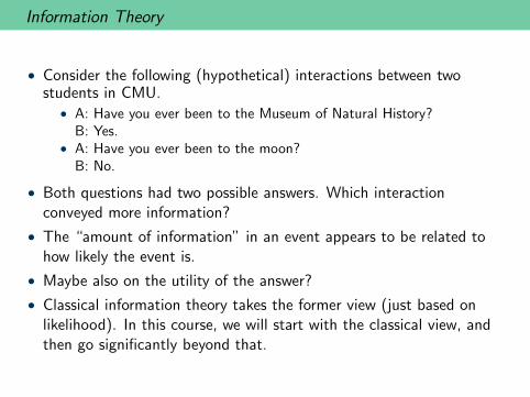
• Consider the following (hypothetical) interactions between twostudents in CMU.
• A: Have you ever been to the Museum of Natural History?B: Yes.
• A: Have you ever been to the moon?B: No.
• Both questions had two possible answers. Which interactionconveyed more information?
• The “amount of information” in an event appears to be related tohow likely the event is.
• Maybe also on the utility of the answer?
• Classical information theory takes the former view (just based onlikelihood). In this course, we will start with the classical view, andthen go significantly beyond that.

Information Theory
• Consider the following (hypothetical) interactions between twostudents in CMU.
• A: Have you ever been to the Museum of Natural History?B: Yes.
• A: Have you ever been to the moon?B: No.
• Both questions had two possible answers. Which interactionconveyed more information?
• The “amount of information” in an event appears to be related tohow likely the event is.
• Maybe also on the utility of the answer?
• Classical information theory takes the former view (just based onlikelihood). In this course, we will start with the classical view, andthen go significantly beyond that.

My personal motivation for going beyond
I was bothered for a very long time, and still am, that informationtheory is largely a theory of communication/compression. A theory ofinformation should be much broader.
• My PhD thesis examined how information theory can solve adistributed control problem (the Witsenhausen counterexample,1967). This is an application of information theory to a problemwhere end-use of information matters: it is defined by theoptimization goal (which is not communication).– also, this is a scalar problem.
• I then examined a problem of communication and computing:minimizing total (comm+compute) energy in a communicationsystem. Shannon capacity does not fall out as the answer.
• Since then, I have examined error correction in distributedcomputing, measures of information flow in neural circuits, andmeasures of fairness in machine learning.
• In no case is Shannon capacity the answer. But in every case, acareful, theoretical approach, yields answers and insights.

Classic applications: Compression and Communication
• Information Theory is the science of measuring of information.
• This science has had a profound impact on sensing, compression,storage, extraction, processing, and communication of information.
• Compressing data such as audio, images, movies, text, sensormeasurements, etc. (Example: We will see the principle behind the‘zip’ compression algorithm in this course.)
• Communicating data over noisy channels such as wires, wireless links,memory (e.g. hard disks), etc.
• Specifically, we will be interested in determining the fundamentallimits of compression and communication. This will shed light onhow to engineer near-optimal systems.
• We will use probability as a “language” to describe and derive theselimits.
• Information Theory has strong connections to Statistics, Physics,Biology, Computer Science, and many other disciplines. Some ofthose connections/applications are the focus of this course.
A General Communication Setting
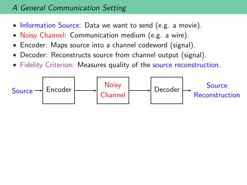
• Information Source: Data we want to send (e.g. a movie).
• Noisy Channel: Communication medium (e.g. a wire).
• Encoder: Maps source into a channel codeword (signal).
• Decoder: Reconstructs source from channel output (signal).
• Fidelity Criterion: Measures quality of the source reconstruction.
Source EncoderNoisy
ChannelDecoder
Source
Reconstruction
• Goal: Transmit at the highest rate possible while meeting thefidelity criterion.
• Example: Maximize frames/second while keeping mean-squared errorbelow 1%.
• Look Ahead: We will see a theoretical justification for the layeredprotocol architecture of communication networks (combine optimalcompression with optimal communication)

A General Communication Setting
• Information Source: Data we want to send (e.g. a movie).
• Noisy Channel: Communication medium (e.g. a wire).
• Encoder: Maps source into a channel codeword (signal).
• Decoder: Reconstructs source from channel output (signal).
• Fidelity Criterion: Measures quality of the source reconstruction.
Source EncoderNoisy
ChannelDecoder
Source
Reconstruction
• Goal: Transmit at the highest rate possible while meeting thefidelity criterion.
• Example: Maximize frames/second while keeping mean-squared errorbelow 1%.
• Look Ahead: We will see a theoretical justification for the layeredprotocol architecture of communication networks (combine optimalcompression with optimal communication)

Bits: The currency of information for communication
• As we will see, bits are a “universal” currency of information forsingle sender, single receiver communication.
• Specifically, when we talk about sources, we often describe their sizein bits. Example: A small JPEG is around 100kB.
• Also, when we talk about channels, we often mention what rate theycan support. Example: A dial-up modem can send 14.4kB/sec.
• But this requires a sophisticated source-channel separation theoremto hold. That theorem holds for point-to-point communication, butbreaks down for even small communication networks. It certainlybreaks down for computing problems, and beyond. So, bits may notbe the currency to express information in your problem.

Applications
The course is aimed to understand informational measures. Inintroductory information theory courses, these are classically examinedonly for compression and communication. This course, on the otherhand, will focus on two other applications specifically:
• Information flow in neural circuits.
• Fairness, Accountability, Transparency, Explainability (FATE) in/ofAI.
There are many other applications where information theory is used,which we will a.s. not discuss in great detail:
• Large deviation theory.
• Deriving minimax lower bounds in statistics.
• Quantifying relevance of data features being sampled from differentsensors.
• Distributed computing.

High Dimensions
• To compress and communicate data close to the fundamental limits,we will need to operate over long blocklengths.
• This is on its face an extremely complex problem: nearly impossibleto “guess and check” solutions.
• Using probability, we will be able to reason about the existence (ornon-existence) of good schemes. This will give us insight into howactually construct near-optimal schemes.
• Along the way, you will develop a lot of intuition for howhigh-dimensional random vectors behave.
• We will now review some basic elements of probability that we willneed for the course.

Probability Review: Events
Elements of a Probability Space (Ω,F ,P):1 Sample space Ω = ω1, ω2, . . . the set of possible outcomes.
2 Set of events F = E1, E2, . . ., where each event is a set ofpossible outcomes (from Ω). We say that the event Ei occurs if theoutcome ωj is an element of Ei.
3 Probability measure P : F → R+, an assignments of probabilities toevents, a function that satisfies
(i) P(∅) = 0.(ii) P(Ω) = 1.(iii) If Ei ∩ Ej = ∅ (i.e. Ei and Ej are disjoint) for all i = j, then
P
( ∞∪i=1
Ei
)=
∞∑i=1
P(Ei) .

Probability Review: Events
Union of Events:
• P(E1 ∪ E2) = P(E1) + P(E2)− P(E1 ∩ E2). (Venn Diagram)
• More generally, we have the inclusion-exclusion principle:
P( n∪
i=1
Ei
)=
n∑i=1
P(Ei)−∑i<j
P(Ei ∩ Ej) +∑
i<j<k
P(Ei ∩ Ej ∩ Ek)
· · ·+ (−1)ℓ+1∑
i1<i2<···<iℓ
P( ℓ∩
m=1
Eim
)+ · · ·
• Very difficult to calculate, often rely on the union bound:
P( n∪
i=1
Ei
)≤
n∑i=1
P(Ei) .

Probability Review: Events
Independence:
• Two events E1 and E2 are independent if
P(E1 ∩ E2) = P(E1)P(E2) .
• The events E1, . . . , En are mutually independent (or justindependent) if, for all subsets I ⊆ 1, . . . , n,
P(∩
i∈IEi
)=
∏i∈I
P(Ei) .

Probability Review: Events
Independence:
• Two events E1 and E2 are independent if
P(E1 ∩ E2) = P(E1)P(E2) .
• The events E1, . . . , En are mutually independent (or justindependent) if, for all subsets I ⊆ 1, . . . , n,
P(∩
i∈IEi
)=
∏i∈I
P(Ei) .

Probability Review: Events
Conditional Probability:
• The conditional probability that event E1 occurs given that event E2
occurs is
P(E1|E2) =P(E1 ∩ E2)
P(E2).
Note that this is well-defined only if P(E2) > 0.
• Notice that if E1 and E2 are independent and P(E2) > 0,
P(E1|E2) =P(E1 ∩ E2)
P(E2)=
P(E1)P(E2)
P(E2)= P(E1) .

Probability Review: Events
Law of Total Probability:
• If E1, E2, . . . are disjoint events such that Ω =
∞∪i=1
Ei, then for any
event A
P(A) =
∞∑i=1
P(A ∩ Ei) =
∞∑i=1
P(A|Ei)P(Ei) .
Bayes’ Law:
• If E1, E2, . . . are disjoint events such that Ω =
∞∪i=1
Ei, then for any
event A
P(Ej |A) =P(A|Ej)P(Ej)
∞∑i=1
P(A|Ei)P(Ei)
.
Probability Review: Random Variables
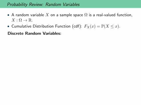
• A random variable X on a sample space Ω is a real-valued function,X : Ω → R.
• Cumulative Distribution Function (cdf): FX(x) = P(X ≤ x).
Discrete Random Variables:
• X is discrete if it only takes values on a countable subset X of R.• Probability Mass Function (pmf): For discrete random variables, wecan define the pmf pX(x) = P(X = x).
• Example 1: Bernoulli with parameter q.
pX(x) =
1− q x = 0
q x = 1 .
• Example 2: Binomial with parameters n and q.
pX(k) =
(n
k
)qk(1− q)n−k k = 0, 1, . . . , n

Probability Review: Random Variables
Continuous Random Variables:
• A random variable X is called continuous if there exists anonnegative function fX(x) such that
P(a < X ≤ b) =
∫ b
afX(x)dx for all −∞ < a < b < ∞ .
This function fX(x) is called the probability density function (pdf)of X.

Probability Review: Random Variables
• Example 1: Uniform with parameters a and b.
fX(x) =
1
b−a a < x ≤ b
0 otherwise.
• Example 2: Gaussian with parameters µ and σ2.
fX(x) =1√2πσ2
e−(x−µ)2
2σ2
• Example 3: Exponential with parameter λ.
fX(x) =
λe−λx x ≥ 0
0 x < 0 .

Probability Review: Random Variables
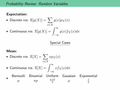
Expectation:
• Discrete rvs: E[g(X)] =∑x∈X
g(x)pX(x)
• Continuous rvs: E[g(X)] =
∫ ∞
−∞g(x)fX(x)dx
Special Cases
Mean:
• Discrete rvs: E[X] =∑x∈X
xpX(x)
• Continuous rvs: E[X] =
∫ ∞
−∞xfX(x)dx
• Bernoulli Binomial Uniform Gaussian Exponential
p np a+b2 µ 1
λ
Probability Review: Random Variables
Expectation:
• Discrete rvs: E[g(X)] =∑x∈X
g(x)pX(x)
• Continuous rvs: E[g(X)] =
∫ ∞
−∞g(x)fX(x)dx
Special Cases
Mean:
• Discrete rvs: E[X] =∑x∈X
xpX(x)
• Continuous rvs: E[X] =
∫ ∞
−∞xfX(x)dx
• Bernoulli Binomial Uniform Gaussian Exponential
p np a+b2 µ 1
λ

Probability Review: Random Variables
Special Cases Continued
mth Moment:
• Discrete rvs: E[Xm] =∑x∈X
xmpX(x)
• Continuous rvs: E[Xm] =
∫ ∞
−∞xmfX(x)dx
Variance:
• Var(X) = E[(X − E[X])2
]= E[X2]−
(E[X]
)2
•Bernoulli Binomial Uniform Gaussian Exponential
p(1− p) np(1− p) (b−a)2
12 σ2 1λ2

Probability Review: Random Variables
Special Cases Continued
mth Moment:
• Discrete rvs: E[Xm] =∑x∈X
xmpX(x)
• Continuous rvs: E[Xm] =
∫ ∞
−∞xmfX(x)dx
Variance:
• Var(X) = E[(X − E[X])2
]= E[X2]−
(E[X]
)2•
Bernoulli Binomial Uniform Gaussian Exponential
p(1− p) np(1− p) (b−a)2
12 σ2 1λ2

Probability Review: Collections of Random Variables
Pairs of Random Variables (X,Y ):
• Joint cdf: FXY (x, y) = P(X ≤ x, Y ≤ y)
• Joint pmf: pXY (x, y) = P(X = x, Y = y) (for discrete rvs)
• Joint pdf: If fXY satisfies
P(a < X ≤ b, c < Y ≤ d) =
∫ b
a
∫ d
cfXY (x, y)dydx
for all −∞ < a < b < ∞ and −∞ < c < d < ∞ then fXY is calledthe joint pdf of (X,Y ). (for continuous rvs)
• Marginalization:pY (y) =
∑x∈X
pXY (x, y)
fY (y) =
∫ ∞
−∞fXY (x, y)dx

Probability Review: Collections of Random Variables
n-tuples of Random Variables (X1, . . . , Xn):
• Joint cdf: FX1···Xn(x1, . . . , xn) = P(X1 ≤ x1, . . . , Xn ≤ xn)
• Joint pmf: pX1···Xn(x1, . . . , xn) = P(X1 = x1, . . . , Xn = xn)
• Joint pdf: If fX1···Xn satisfies
P(a1 < X1 ≤ b1, . . . , an < Xn ≤ bn)
=
∫ b1
a1
· · ·∫ bn
an
fX1···Xn(x1, . . . , xn)dxn · · · dx1
for all −∞ < ai < bi < ∞ then fX1···Xn is called the joint pdf of(X1, . . . , Xn).

Probability Review: Collections of Random Variables
Independence of Random Variables:
• X1, . . . , Xn are independent ifFX1···Xn(x1, . . . , xn) = FX1(x1) · · ·FXn(xn)∀x1, x2, . . . , xn
• Equivalently, we can just check if
pX1···Xn(x1, . . . , xn) = pX1(x1) · · · pXn(xn) (discrete rvs)
fX1···Xn(x1, . . . , xn) = fX1(x1) · · · fXn(xn) (continuous rvs)

Probability Review: Collections of Random Variables
Conditional Probability Densities:
• Given discrete rvs X and Y with joint pmf pXY (x, y), theconditional pmf of X given Y = y is defined to be
pX|Y (x|y) =
pXY (x,y)pY (y) pY (y) > 0
0 otherwise.
• Given continous rvs X and Y with joint pdf fXY (x, y), theconditional pdf of X given Y = y is defined to be
fX|Y (x|y) =
fXY (x,y)fY (y) fY (y) > 0
0 otherwise.
• Note that if X and Y are independent, then pX|Y (x|y) = pX(x) orfX|Y (x|y) = fX(x).

Probability Review: Collections of Random Variables
Linearity of Expectation:
• E[a1X1 + · · ·+ anXn] = a1E[X1] + · · ·+ anE[Xn] even if the Xi
are dependent.
Expectation of Products:
• If X1, . . . , Xn are independent, thenE[g1(X1) · · · gn(Xn)] = E[g1(X1)] · · ·E[gn(Xn)] for anydeterministic functions gi.

Probability Review: Collections of Random Variables
Conditional Expectation:
• Discrete rvs: E[g(X)|Y = y] =∑x∈X
g(x)pX|Y (x|y)
• Continuous rvs: E[g(X)|Y = y] =
∫ ∞
−∞g(x)fX|Y (x|y)dx
• E[Y |X = x] is a number. This number can be interpreted as afunction of x.
• E[Y |X] is a random variable. It is in fact a function of the randomvariable X. (Note: A function of a random variable is a randomvariable.)
• Lemma: EX
[E[Y |X]
]= E[Y ].

Probability Review: Collections of Random Variables
Conditional Independence:
• X and Y are conditionally independent given Z if
pXY |Z(x, y|z) = pX|Z(x|z)pY |Z(y|z) (discrete rvs)
fXY |Z(x, y|z) = fX|Z(x|z)fY |Z(y|z) (continuous rvs)

Probability Review: Collections of Random Variables
Markov Chains:
• Random variables X, Y , and Z are said to form a Markov chainX → Y → Z if the conditional distribution of Z depends only on Yand is conditionally independent of X.
• Specifically, the joint pmf (or pdf) can be factored as
pXY Z(x, y, z) = pX(x)pY |X(y|x)pZ|Y (z|y) (discrete rvs)
fXY Z(x, y, z) = fX(x)fY |X(y|x)fZ|Y (z|y) (continuous rvs) .
• X → Y → Z if and only if X and Z are conditionally independentgiven Y .
• X → Y → Z implies Z → Y → X (and vice versa).
• If Z is a deterministic function of Y , i.e. Z = g(Y ), thenX → Y → Z automatically.

Probability Review: Inequalities
Convexity:
• A set X ⊆ Rn is convex if, for every x1,x2 ∈ X and λ ∈ [0, 1], wehave that λx1 + (1− λ)x2 ∈ X .
• A function g on a convex set X is convex if, for every x1,x2 ∈ Xand λ ∈ [0, 1], we have that
g(λx1 + (1− λ)x2) ≤ λg(x1) + (1− λ)g(x2) .
• A function g is concave if −g is convex.
Jensen’s Inequality:
• If g is a convex function and X is a random variable, then
g(E[X]) ≤ E
[g(X)
]

Probability Review: Inequalities
Markov’s Inequality:
• Let X be a non-negative random variable. For any t > 0,
P(X ≥ t) ≤ E[X]
t.
Chebyshev’s Inequality:
• Let X be a random variable. For any ϵ > 0,
P(∣∣X − E[X]
∣∣ > ϵ)≤ Var(X)
ϵ2.

Probability Review: Inequalities
Markov’s Inequality:
• Let X be a non-negative random variable. For any t > 0,
P(X ≥ t) ≤ E[X]
t.
Chebyshev’s Inequality:
• Let X be a random variable. For any ϵ > 0,
P(∣∣X − E[X]
∣∣ > ϵ)≤ Var(X)
ϵ2.

Probability Review: Inequalities
Weak Law of Large Numbers (WLLN):
• Let Xi be a sequence of independent and identically distributed(i.i.d.) random variables with finite mean, µ = E[Xi] < ∞.
• Define the sample mean Xn =1
n
n∑i=1
Xi.
• For any ϵ > 0, the WLLN implies that
limn→∞
P(∣∣Xn − µ
∣∣ > ϵ)= 0 .
• That is, the sample mean converges (in probability) to the truemean.
Probability Review: Inequalities
Strong Law of Large Numbers (SLLN):
• Let Xi be a sequence of independent and identically distributed(i.i.d.) random variables with finite mean, µ = E[Xi] < ∞.
• Define the sample mean Xn =1
n
n∑i=1
Xi.
• The SLLN implies that
P(
limn→∞
Xn = µ)
= 1 .
• That is, the sample mean converges (almost surely) to the truemean.