18 oceanic analogues of large-scale atmospheric motions · oceanic analogues of large-scale...

18Oceanic Analoguesof Large-scaleAtmospheric Motions

Jule G. Charney andGlenn R. Flierl

18.1 Introduction

Newton (1687, book 2, propositions 48-50) and Laplace(1799) were aware that the principles governing theocean tides would also govern the atmospheric tides.Helmholtz (1889) showed that ocean waves and billowclouds were manifestations of the same hydrodynamicinstability, and he speculated that storms were causedby a similar instability. Had he known the structure ofthe Gulf Streams meanders, he might have speculatedon their dynamic similarities to storms as well. Suchintercomparisons were natural to the great hydrody-namicists of the past who took the entire universe offluid phenomena as their domain. Although a degreeof provincialism was introduced in the late nineteenthand early twentieth centuries by the exigencies ofweather forecasting, it was just the practical require-ments of weather observation that stimulated the de-velopment of modem dynamic meteorology and led tothe deepening of its connections with physical ocean-ography. The recent explosive growth of the three-di-mensional data base, the exploration of other planetaryatmospheres, and the resulting increase in theoreticalactivity have greatly extended the list of ocean-atmos-phere analogues. Indeed, it is now no exaggeration tosay that there is scarcely a fluid dynamical phenomenonin planetary atmospheres that does not have its coun-terpart in the oceans and vice versa. This had led tothe discipline, geosphysical fluid dynamics, whoseguiding principles are intended to apply equally tooceans and atmospheres.

Within this discipline the dominance of the earth'srotation defines a subclass of large-scale phenomenawhose dynamics may for the most part be derived fromquasi-geostrophy. For several years the authors haveconducted a graduate course at MIT on the dynamicsof large-scale ocean and atmospheric circulations inthe belief that a parallel consideration of large-scaleoceanic and atmospheric motions would broaden therange of our students' experience and deepen their un-derstanding of the principles of fluid geophysics. C.-G.Rossby (1951) put the matter well:

It is fairly certain that the final formulation of a com-prehensive theory for the general circulation of theatmosphere will require intimate cooperation betweenmeteorologists and oceanographers. The fundamentalproblems associated with the heat, mass and momen-tum transfer at the sea surface concern both these sci-ences and demand a joint effort for their solution. How-ever, an even stronger reason for that pooling ofintellectual resources .. . may be found in the fact thatthe various theoretical analyses of the large-scaleoceanic and atmospheric circulation patterns whichhave been called into being by our sudden wealth ofobservational data, appear to have so much in commonthat they may be looked upon as different facets of onebroad general study, the ultimate aim of which might

504Jule G. Chamey and Glenn R. Flierl

_ ___ _ ___

be described as an attempt to formulate a comprehen-sive theory for fluid motion in planetary envelopes.

He went on to say that "comparisons between thecirculation patterns in the atmosphere and in theoceans provide us with a highly useful substitute forexperiments with controlled variations of the funda-mental parameters."

Needless to say, we subscribe to Rossby's views andtherefore have willingly undertaken the task of review-ing the fluid dynamics of a number of phenomena thathave found explanation in one medium and are deemedto have important analogues in the other. Where theanalogues have already been explained, we have given abrief review of some of their salient features, but wherelittle is known, we have not refrained from interpolat-ing simple models or speculations of our own. In doingso, we were aware that the subject has grown so largethat it includes most of geophysical fluid dynamics,and that, even if it were limited to large-scale, quasi-geostrophic motions, it could not be encompassed ina review article of modest size. At least two excellentreview articles on this topic, by N. Phillips (1963) andby H.-L. Kuo (1973), have already appeared, and thereis now a text by Pedlosky (1979a) on geophysical fluiddynamics. For these reasons we have decided tto limitourselves to a small number of topics having todo primarily with disturbances of the principal at-mospheric and oceanic currents, their propagationcharacteristics, their interactions with the embed-ding currents, and, to a lesser degree, with their self-interactions.

It is perhaps no accident that both Phillips and Kuoare meteorologists. Dynamic meteorology has bene-fited from a wealth of observational detail that hasbeen denied to physical oceanography. Consequently,meteorologists have been the first to observe and ex-plain many typical large-scale phenomena. This has byno means always been the case, but it has been sosufficiently often to justify the title of our review.

18.2 The General Circulations of Oceans andAtmospheres Compared

If it had been possible in a meaningful way, it wouldhave been useful and instructive to make detailed dy-namical comparisons of the general circulations of theatmosphere and oceans. This has not been so, and wemust content ourselves with a few general remarks.Because of its relative transparency to solar radiation,the earth's atmosphere is heated from below; theoceans, like the relatively opaque atmosphere of Venus,are heated from above. The differential heating of theatmosphere produces a mean circulation that carriesheat upward and poleward. Its baroclinic instabilitiesdo likewise. These heat transports, combined with in-

ternal radiative heat transfer, tend to stabilize the at-mosphere statically, and their effects are augmented bymoist convection which drives the temperature lapse-rate toward the moist-adiabatic. The net result is thatthe atmosphere is rather uniformly stable for dry proc-esses up to the tropopause. Above the tropopause, it ismade increasingly more stable by absorption of solarultraviolet radiation in the ozone layer. The oceans arerendered statically stable by heating from above, butheating cannot take place everywhere because theoceans, unlike the atmosphere, cannot dispose of in-temal heat by radiation to space; they must carry itback to the surface layers, where it can be lost bysurface cooling. The most stable parts of the oceans arein the subtropical gyres, where the oceans are heatedand Ekman pumping transfers the heat downward. Theleast stable parts are in the polar regions, where coldwater is formed and carried downward by convection.The atmospheric troposphere has sometimes beencompared with the waters above the thermocline, thetropopause with the thermocline, and the stratospherewith the deep waters below the thermocline (cf. De-fant, 1961b). This comparison may be justified by thefact that it is in the atmospheric and oceanic tropo-spheres that the horizontal temperature gradients andthe kinetic and potential energy densities are greatest.But from the standpoint of static stability, the absorp-tion of radiation at the surface of the oceans makes itsupper layers more analogous to the stratosphere. Thestatic stability for the bulk of the atmosphere andoceans is determined by deep convection occurring insmall regions. The analogy between deep convectionin the atmosphere and deep convection in the oceansis between the narrow intertropical convergence zonesover the oceans and the limited areas of cumulus con-vection over the tropical continents on the one hand,and the limited regions of deep-water formation in thepolar seas on the other. From this standpoint, the oceanwaters below the thermocline are more analogous tothe atmospheric troposphere. Both volumes comprisemore than 80% of the total by mass and both arecontrolled by deep convection.

It is remarkable that the regions of pronounced risingmotion in the atmosphere and sinking motion in theoceans are so confined horizontally. Stommel (1962b)was the first to offer an explanation for the smallnessof the regions of deep-water formation. His work mo-tivated several attempts to explain the asymmetries inthe circulation of a fluid heated differentially fromabove or below. We may cite as examples the experi-mental work of H. T. Rossby (1965) and the theoreticalwork of Killworth and Manins (1980) on laboratoryfluid systems, and the papers of Goody and Robinson(1966) and Stone (1968) on the upper circulation ofVenus. Because of its cloudiness, Venus has been as-sumed to be heated primarily from above, although it

505Oceanic Analogues of Atmospheric Motions

now is known that sunlight does penetrate into thelower Venus atmosphere and that the high tempera-tures near the surface are due to a pronounced green-house effect (Keldysh, 1977; Young and Pollack, 1977;Tomasko, Doose, and Smith, 1979). When a fluid isheated from below, the rising branches are found to benarrow and the sinking branches broad; when it isheated from above the reverse is true. One may offerthe qualitative explanation that it is the branch of thecirculation that leaves the boundary and carries withit the properties of the boundary that has the greatestinfluence on the temperature of the fluid as a whole:convection is more powerful than diffusion. In the caseof differential heating from below, the rising warmbranch causes most of the fluid to be warm relative tothe boundary and therefore gravitationally stable ex-cept in a narrow zone at the extreme of heating wherethe intense rising motion must occur. In the case ofdifferential heating from above, the sinking cold branchcauses the bulk of the fluid to be cold and gravitation-ally stable except in a narrow region at the extreme ofcooling where the intense sinking motion must occur.Theoretical models of axisymmetric, thermally driven(Hadley) circulations in the atmosphere (Charney,1973) show the same effect: a narrow rising branch anda broad sinking branch. This effect is strengthened bycumulus convection (Charney, 1969, 1971b; Bates,1970; Schneider, 1977). The narrow rising branch ofthe Hadley circulation directly controls the dynamicand thermodynamic properties of the tropics and sub-tropics and indirectly influences the higher-latitudecirculations. Similarly, the small sinking branches ofthe ocean circulation determine the near-homogeneousdeep-water properties as well as some of the interme-diate-water properties. But there is a difference: weknow how the heat released in the ascending branchof the Hadley circulation is disposed of; we do notknow how the cold water in the abyssal circulation isheated. Whatever the process, the existence of a pre-ponderant mass of near-homogeneous water at depthforces great static stability in the shallow upper regionsof the ocean. It demands a thermocline.

Again we have an analogy between the upper circu-lation of the oceans and the upper circulation of Venus.Rivas (1973, 1975) has shown that the intense circu-lation of Venus is confined to a thin layer within andjust below the region of intense heating and cooling byradiation. The more or less independent circulationproduced by the separate heat sources of the atmos-pheric stratosphere is similarly analogous to the upperocean circulation. And here there is an atmosphere-ocean analogy pertaining to our knowledge of transferprocesses. While the mechanisms of heat transfer inthe stratosphere are fairly well known, the mechanismof transfer of thermally inactive gases or suspended

particles is not, for the latter involves a knowledge ofparticle trajectories, which are not easily determined.The large-scale eddies in the atmosphere, insofar asthey are nondissipative, cannot transfer a conservedquantity across isentropic surfaces. Thermal dissipa-tion is required for parcels to move from the low-en-tropy troposphere to the high-entropy stratosphere.Atmospheric chemists sometimes postulate an ad hocturbulent diffusion to explain the necessary verticaltransfers of such substances as the oxides of nitrogenand the chlorofluoromethanes into the ozone layers.But it is doubtful whether this type of diffusion isneeded to account for the actual transfer, because therealready exists the nonconservative mechanism of ra-diative heat transfer, and this, together with the large-scale eddying motion, can by itself account for thetransfers (Andrews and McIntyre, 1978a; Matsuno andNakamura, 1979). The analogous oceanic problem hasalready been mentioned: how is heat or salt transferredfrom the deep ocean layers into the upper wind-stirredlayers? The cold deep water produced in the polar seasand the intermediate salty water produced in the Med-iterranean Sea must eventually find their way by dis-sipative processes to the surface, where they can beheated or diluted. While a number of internal dissipa-tion mechanisms have been proposed in a speculativeway (double diffusion, low-Richardson-number insta-bility zones, internal-wave breaking) one may invokeOccam's razor, as has been done so successfully toexplain the Gulf Stream as an inertial rather than africtional boundary layer (Chamey, 1955b; Morgan,1956) and postulate no internal dissipative mechanismat all. Then, outside of the convective zones, propertieswill be advected by the mean flow or by eddies alongisentropic surfaces, and move from one such surface toanother only at the boundaries of the ocean basinswhere we may assume turbulent dissipation does oc-cur. It would be interesting to see how far one couldgo with boundary dissipation alone. Welander (1959)and Robinson and Welander (1963) have taken a firststep by investigating the motions of a conservativesystem communicating only with an upper mixedlayer.

18.3 The Transient Motions

Meteorologists, pressed with the necessity of forecast-ing the daily weather, have always been concernedwith the transient motions of the atmosphere. At-tempts to understand the processes leading to growth,equilibration, translation and decay of these "synoptic-scale" (order 1000 km) eddies' have produced theoriesof baroclinic instability (Charney, 1947; Eady, 1949),Rossby wave motion (Rossby et al., 1939; Haurwitz,1940b) and Ekman pumping (Charney and Eliassen,1949). It was first recognized by Jeffreys (1926) and

506Jule G. Charney and Glenn R. Flierl

__r __� _ __1_1__�

demonstrated conclusively by Starr (1954, 1957) andBjerknes (1955, 1957) that the dynamics of the meancirculation are strongly influenced by the transports ofheat and zonal momentum by the eddies [for a reviewof these developments, see Lorenz (1967)]. This hasprompted research on eddy dynamics and also on theparameterization of eddy fluxes (cf. Green, 1970;Rhines, 1977; Stone, 1978; Welander, 1973).

The study of eddy motions in the ocean is a newdevelopment. Although the existence of fluctuationsin the Gulf Stream was reported by early observerssuch as Laval (1728) and Rennell (1832), actual predic-tion of ocean eddies has never been a particularly prof-itable exercise (perhaps the recent interest of yachts-men in Gulf Stream rings may presage a change). Theserious study of deep ocean fluctuations really beganwith M. Swallow (1961), Crease (1962), and J. Swallow(1971). At this point, oceanographers began to realizethat the mid-ocean variable velocities were not, asmight perhaps have been reasonably inferred from at-mospheric experience, comparable to the mean flowsbut rather were an order of magnitude larger. This hasspurred intensive experimental and theoretical inves-tigations of the dynamics of the oceanic eddies andtheir roles in the general circulation (see chapter 11).

Comparisons between the oceanic and atmosphericeddies may be made in respect to their generation,propagation, interaction (both eddy-mean flow andeddy-eddy) and decay. In the sections below we shalldescribe some of the theoretical approaches to theseproblems.

In the atmosphere, energy conversion estimates (cf.Oort and Peixoto, 1974) clearly show a transformationof zonal-available potential energy into eddy-availablepotential energy, then into eddy kinetic energy andfinally into heat by dissipation, with some transferfrom eddy to zonal kinetic energy. The similarity ofthe growth phase of this cycle to that exhibited in thetheory of small traveling perturbations of a baroclini-cally unstable (but barotropically stable) flow, leadsnaturally to the identification of the source of thewaves as the baroclinic instability of the zonal flow.This idea has been supported further by the fact thatthe energy spectrum has peaks near zonal wavenumbersix, which simple models predict to be the most rapidlygrowing wavenumber. However, attempts to applythese models directly to the atmosphere lead to prob-lems: one expects that nonuniform mean flows, non-homogeneous surface conditions, variable horizontaland vertical shears, etc., will alter the dynamics; andone may also wonder about the applicability of thesmall perturbation-normal mode approach.

The topographically and thermally forced standingeddies also draw upon zonal available potential energy(Holopainen, 1970). The processes by which they dothis are not yet clearly understood; they may be related

to the form-drag instability to be described in section18.7.3. The standing eddies, like the transient eddies,also transport heat and momentum.

Overall energetic analyses have not been applied tooceanic data. However, budgets for basin-averaged ki-netic and potential energy have been calculated for the"eddy-resolving general circulation models." These arereviewed by Harrison (1979b). In all but one of the 21cases he considered, the eddy kinetic energy came fromboth mean kinetic and mean potential energy. Collec-tively, the eddies seem to be acting as dissipativemechanisms, but Harrison cautions that because themodel statistics are inhomogeneous, the overall resultsmay not be representative of the actual dynamics inany limited region. Indeed, the eddies may be acting asa negative viscosity in parts of the domain. Thus, Hol-land (1978) suggests that the eddies generated in theupper layer of his two-layer model drive the mean flowsin the lower layer.

Oceanographers have examined local energy bal-ances. The best known of these studies, by Webster(1961 a), has often been interpreted as an indication thatthe Gulf Stream is accelerated by the eddies. However,Schmitz and Niiler (1969) have pointed out that thecross stream-averaged value of u'v'vx is not distin-guishable from zero, so that Webster's results may bean indication merely of transfer of energy from theoffshore to the onshore side of the jet and not a mean-flow generation. Even this result is not unambiguous,since the divergence term (u'v'v), is not small com-pared to the terms -(u'vv') and u'v'v,, representing,respectively, the eddy-mean flow and the mean flow-eddy conversions. The same problem occurs in at-tempts to compute regional energy budgets in numer-ical models (cf. Harrison and Robinson, 1978) unlessconsiderable care is taken.

The conversion of mean-flow potential energy issometimes inferred from the tilting of the phase linesof the temperature wave with height. This tilt is takenas evidence that the wave is growing by baroclinicinstability of the mean flow. Here one must be careful:it is the lagging of the temperature wave behind thepressure wave and the consequent tilting of the phaseline of the pressure trough toward the cold air that isimportant; the temperature phase line may tilt in anydirection or not at all. Thus in the Eady model ofbaroclinic instability the temperature wave has theopposite slope from the pressure wave, whereas in theChamey model it has the opposite slope at low levelsand the same slope at high levels (Chamey, 1973, chap-ter IX). It is appropriate, then, to caution that theoceanically most readily available quantity, the phasechange of the buoyancy (or entropy) with height, maynot lead to a straightforward determination of the signof the buoyancy flux.


This discussion should make it clear that very littleis settled concerning the source of the eddies in theocean and their effects on the mean flow. "Local" gen-eration mechanisms, such as baroclinic or barotropicinstability, flow over topography, and wind forcing arestill being considered, and atmospheric analogues aremuch in mind. But the fact that the transient atmos-pheric perturbation velocities are comparable to thoseof the mean flow, whereas the particle speeds for mid-ocean mesoscale eddies are an order of magnitudegreater than the mean speeds, suggests that energy maybe generated only in limited regions (e.g., the westernboundary currents) and propagate from there to otherregions.

Oceanic eddies propagate in much the same manneras atmospheric eddies, although there are differencesbecause of the upper-surface boundary conditions: at-mospheric waves may propagate upward without re-flection, whereas oceanic waves are reflected at theupper boundary. In the atmosphere, the potential vor-ticity gradients associated with the mean flow play animportant role in determining the vertical structureand horizontal propagation for atmospheric waves,whereas this role is played primarily by the gradient ofthe earth's vorticity for mid-oceanic waves.

The interaction mechanisms may be classified aswave-mean flow interactions and wave-wave inter-actions. As mentioned above, the concrete evidence forsignificant wave-mean flow interaction is muchgreater for the atmosphere than for the ocean. There isnot, of course, much oceanic data-Reynolds stresseshave been calculated only along a few north-southsections (Schmitz, 1977). Moreover, these records arenot very long and the spatial resolution is not sufficientto compute accurate gradients of the Reynolds stresses(given the great inhomogeneity).

The wave-wave interactions, however, seem similarin the two media. The crucial parameter is the Rossbywave steepness parameter M = U/1L2, which distin-guishes wavelike regimes (M < 1) from more turbulent(M > 1) regimes as illustrated in the experiments ofRhines (1975).2 The oceans are similar to the atmos-phere in that this parameter is of order unity for both,although it appears to vary considerably from oneoceanic region to another.

The physical mechanisms for dissipation of atmos-pheric and oceanic eddies are thought to be similarwith respect to bottom friction and transfer of energyto gravity wave motions or turbulence (though radia-tion is a further factor in damping atmosphere waves),but their relative importance may be quite different.The crucial differences for the large-scale circulationsbetween the atmosphere and the ocean may not be inthe details of the dissipation mechanisms but rather intheir overall time scales. In the atmosphere, dampingtimes are of the order of a few days, comparable to the

eddy velocity advection time LIU, whereas the damp-ing time in the ocean may be as long as several years(cf. Cheney and Richardson, 1976) while the advectiontime is of the order of a week.

18.4 The Geostrophic Formalism

18.4.1 The Development of the GeostrophicFormalismThe discovery that the atmospheric winds are approx-imately geostrophic is usually attributed to Buys Ballot(1857). Ferrel (1856) suggested that ocean currentsmight also have this property. But it took nearly acentury before this knowledge was used dynamically.Because the geostrophic and hydrostatic equations ex-press only a condition of balance, it is necessary toconsider the slight imbalances produced by forcing,dissipation, and transience in order to predict the ev-olution and to understand the processes that maintainthe balance. One of the first to exploit geostrophy wasBjerknes (1937) in a seminal work on the upper tropos-pheric long waves and their role in cyclogenesis. Basinghis analysis on semiempirical considerations of thegradient wind and the variation with latitude of theCoriolis parameter, he gave the first explanation of theeastward propagation of the upper wave at a speedslower than the mean wind. It was this work that ledRossby et al. (1939) to their vorticity analysis of theupper wave as an independent entity in planar flow.Chamey (1947) and Eady (1949) derived quasigeos-trophic equations in their analyses of baroclinic insta-bility for long atmospheric waves. General derivationsof these equations for arbitrary motions were presentedby Charney (1948), Eliassen (1949), Obukhov (1949),and Burger (1958). A particularly simple form whichwill be used in this review was given by Chamey (1962)and Charney and Stem (1962).

In addition to these commonly used approximations,there have been a number of simplifications of theequations of motion which apply the concept of near-geostrophic balance in a less restrictive form. Whenflows become nongeostrophic in one horizontal dimen-sion while remaining geostrophic in the other, as infrontogenesis, flow over two-dimensional mountainbarriers, and in the western boundary currents of theoceans, a set of "semigeostrophic" equations derivedfrom Eliassen's original formulation has often beenfound useful (Robinson and Niiler, 1967; Hoskins,1975). Both the quasi- and semigeostrophic equationsare special cases of the "balance equations" proposedby Bolin (1955), Chamey (1955c, 1962), P. Thompson(1956), and Lorenz (1960). They may be derived fromthe consideration that in a large class of atmosphericflows the constraints of the earth's rotation and/orgravitational stability so inhibit vertical motion thatthe horizontal flow, even when it is not quasi-geo-


strophic, remains quasi-nondivergent. The equationsderived by Eliassen (1952) for slow thermally and fric-tionally driven circulations in a circular vortex are aspecial case of the balance equations; they representthe laws of conservation of angular momentum andentropy and the requirement of equilibrium among themeridional components of the pressure, gravity, andcentrifugal forces. For the equilibrium condition to bevalid, the flow must be gravitationally and inertiallystable. This implies that the potential vorticity mustbe positive in the northern hemisphere and negative inthe southern hemisphere, and it may be shown thatthis condition on the potential vorticity is also requiredfor the general asymmetric case.

One must also explain why external sources of en-ergy excite quasi-geostrophic flows rather than gravitywave motions to begin with and why so little energyis transferred by nonlinear interactions into the gravitymodes afterward. The tendency toward geostrophy issometimes explained as an adjustment of an initiallyunbalanced flow by radiation of gravity waves in themanner discussed by Rossby (1938) (see also Blumen,1968). However, since much of the forcing is appliedslowly, rather than impulsively, the calculations ofVeronis and Stommel (1956), who consider the natureof the exciting forces, are perhaps more relevant. Theyshowed that the flows will be geostrophically balancedwhen the forcing period is very large compared to theinertial period. Thus we expect most of the energy willgo into geostrophic motions.

The question of how much transfer occurs from geo-strophic to nongeostrophic motions through nonlinearinteractions remains a matter of concern. Errico's(1979) work suggests that equipartition of energy be-tween gravity waves and geostrophic motions will oc-cur in a conservative, rotating system in statisticalequilibrium at sufficiently high energy. But in dissi-pative systems resembling the atmosphere and oceans,the energy will remain in the geostrophic modes be-cause the gravity waves are dissipated on time scalesthat are small in comparison with those of their gen-eration. This problem has elements in common withthe so-called initialization problem in numericalweather prediction: to find initial values of a flow fieldthat are at once compatible with the incomplete dataand at the same time minimize the initial gravity-waveenergy and its production rate (cf. Machenhauer, 1977;Daley, 1978).

The problems of transfer from geostrophic into grav-ity-wave energy are related to those of the productionof hydrodynamic noise by a turbulent flow, first stud-ied by Lighthill (1952). An excellent review is presentedby Ffowcs Williams (1969). Here the problem is tocalculate the generation of acoustic energy in a tur-bulent flow in which most of the energy resides innondivergent motions. Since the turbulence is confined

within a limited domain and radiates sound waves intothe surrounding medium, there is no possibility ofequipartition. An atmospheric or oceanographic anal-ogy to the Lighthill problem would be the generationof internal gravity waves by turbulence in a planetaryboundary layer (Townsend, 1965), except that here thegeneration takes place, not within the layer, but at itsinterface with the neighboring stable stratum.

Physicists, too, have struggled with problems inwhich many scales interact simultaneously (cf. Wilson,1979), but it is not known whether their renormaliza-tion group methods can be usefully applied to atmos-pheric or oceanic problems.

18.4.2 Natural Oscillations of the Atmosphere andOceansThe quasi-geostrophic equations have been derived forranges of the various nondimensional parameters thatare of interest in dealing with particular classes of at-mospheric and oceanic motions. It is not to be expectedthat they will remain uniformly valid throughout theentire range of rotationally dominated flows, evenwhen the primary balance is geostrophic. Burger (1958)was the first to point out explicitly that when the 3-plane approximation L/a << 1, where L is the charac-teristic horizontal scale and a is the radius of the earth,is no longer valid, the dynamics of the motion changeradically. On a planetary scale the motion becomeseven more strongly geostrophic, but the vorticity bal-ance changes. Sverdrup (1947) made implicit use of thisdynamics in his treatment of the steady, wind-drivencirculation of the oceans, and it has been used for thetreatment of steady thermohaline circulations of theoceans by Robinson and Stommel (1959) and Welander(1959). [See the review articles by Veronis (1969,1973b), and chapter 5.]

In this section we present a classification of naturaloscillations in atmospheres and oceans in which rota-tion plays a dominant role, paying special attention tothe domain of validity of the 3-plane, quasi-geostrophicequations, the nature of the oscillations for whichthese equations are not valid, and the effects of nonlin-earity, which, especially in the oceans, may give riseto solitary wave behavior.

Although the wave forcing is very different in theoceans and the atmosphere, there are many features ofthe responses that strongly resemble one another. Thisresults because the response of a forced system dependsstrongly on the characteristics of the natural oscilla-tions, and these have many similarities in the atmos-phere and oceans. We shall discuss both the linear andnonlinear natural (unforced and nondissipative) oscil-lations of a simple model consisting of a single-layer,homogeneous, incompressible fluid with a free surfaceon a /3-plane. This is a much oversimplified model, andwe must regard the conclusions to be drawn merely as


suggestions of the way in which the fully straspherical system would behave. The most interimplication-that the dynamics of scales intermbetween the Rossby radius and the radius of themay be dominated by solitary waves, in which near density advection balances linear dispersifects-may not be very sensitive to the partmodel chosen.

At the beginning of each subsection to follcshall describe briefly the methods used and the obtained in order to make it possible for the reaomit the more detailed derivations. We begin tIcussion of the normal modes of oscillation by sthe shallow-water equations in a reference frameing with the wave. The Bernoulli and potential ity integrals then give two equations relating thestreamfunction 4 to the surface elevation ,r abo'mean level H. These equations contain an unkfunctional X, the Bernoulli function, which we cby requiring the equations to hold for vanishing'1n

We then obtain two coupled nonlinear partialential equations defining an eigenvalue problem Iphase speed c. These equations have three nondsional parameters: E, a Rossby number measuribratio of the inertial to the Coriolis forces; 3, astability parameter measuring the ratio of themation scale LR to the wave scale L; and , th{tional change in the Coriolis parameter over thescale. In the standard quasi-geostrophic range (E -1, 3 - 1), when motions have small Rossby nurlength scales comparable to the deformation rthe Bernoulli equation to lowest order is simply ament of geostrophic balance, and the potential volequation becomes the linear quasi-geostrophicequation.

The single-layer equations will be written in dsional form

DuDt- Ifo + 13y)v = -gq,

DvD+ (f + fo + y)u = -g,D

Dt + (H + q)(ux + v) = 0,

D a a aDt= t ox ay'

where qr is the displacement of the surface fromsea level, H is the mean depth of the fluid, ggravitational acceleration (we shall use a reducedity value here), f, = 2c1 sin e, , = 2(1 cos O/a, y =where 0 is the central latitude and AO is the axdistance from 0. In nondimensional form thesetions become

Du - 1 + Ay)v = -71,Dt

3 Dv + (1 + 3y)u = -*!Y,

Dt + (1 + r)(u, + vy) = 0,

(18.2)

D a a aDt at f S + V a Y

where both x and y are scaled by L, 'r is scaled geo-strophically by LUfo/g, and the nondimensional param-eters are i = fL/fo = L cot 0/a L/LA, e = U/foL, andS = gH/f2L2 - L/L 2. We have also introduced thedefinitions of two scales which turn out to be impor-tant in determining the boundaries between varioustypes of behavior: the -scale Lp = fo/f = a tan 0, atwhich variations in the vertical component of theearth's angular velocity are order of the angular veloc-ity itself, and the Rossby radius of deformation LR =Vg-H/fo (Rossby, 1938). We shall use 3500 km for L;(corresponding to 0 - 300) and 50 km (oceanic) or 1000km (atmospheric) for LB. We have also made the choiceof the long-wave period for the time scale so that T =L L-.

The quasi-geostrophic potential vorticity equationmay be derived by expanding (18.2) in powers of for

- E << 1 and 3 - 1, giving

[at +(S a _ 71Y a77X ) (V2 _ 3 + YIf)= laOX.I(

_= 0. (18.3)

The failure of this equation at small space or timescales and near the equator is well known. Meterorol-ogists since Burger (1958) have also recognized thatsome larger than synoptic-scale motions also do notevolve according to this equation. Rather, the appro-priate equations are derived by assuming 3 and to besmall (because L is very large) and i to be of order 1.The resulting velocities remain geostrophic:

1u = 1 +

1v = 1 + , X (18.4)

(18.1) and the height field evolves according to

at 71 11 +2 = ) (18.5)

Equations (18.3) and (18.5) have very different proper-ties: the quasi-geostrophic equation has uniformlypropagating linear-wave solutions which are essen-tially dispersive even at large amplitudes (cf. Mc-Williams and Flierl, 1979), while the Burger equationdoes not have uniformly propagating linear-wave so-lutions and initial disturbances steepen because of non-

51OJule G. Chamey and Glenn R. Flierl

_ _·___ _I ___� ��_ ______

linearity. We shall demonstrate that there is an inter-mediate band of length scales in which nonlinearityand dispersion can balance to give cnoidal or solitarywaves. In the ocean, as we shall see, the change fromquasi-geostrophic to intermediate dynamics to Burgerdynamics occurs at a relatively small scale because thedeformation radius is so small compared to the radiusof the earth.

We may elucidate these differences by consideringthe shallow-water equations under the assumption thatthe motions are translating steadily at speed c:

(v -ci).Vv + (f0 + py) x v = -gVq,(18.6)

(v -ci).Vr + (H + )V-v = 0,

where x and 2 are unit vectors in the positive x and zdirections. We may define a transport streamfunctionin the coordinate system moving with the wave

(v -c)(H + q) = £ x Vw

and write the Bernoulli and potential vorticity integralsof motion:

IV( + cHy)12 + g(H + ) + c(H + )2 (oy + )

= (H + i7)2g6(4 + cHy), (18.7)

V. V(4 + cHy) + (fo + fly) = (H + 9l)t'(0 + cHy),

where we have isolated the wave part of the stream-function = - cHy. We require that (18.7) hold asd, 1 -7- 0; this determines the Bernoulli functional

,9(Z) = C2 + gH + Z + Z2.2 H 2cH2 (18.8)

The choice of a single-valued, well-behaved Bernoullifunctional implies that only motions which reducesmoothly to linear waves will be considered; thus thesolutions of Stern (1975b) or Flierl, Larichev, Mc-Williams, and Reznik, (1980) which involve closedstreamlines and a multiple-valued R will not be ex-amined here.

In nondimensional form, equations (18.7) become

--2 1 +- Sc1 + 1 + 7)

= 82Sc1 (1 + 1) + 0 + ) (1 + 7)0

<Co

4

(18.9)E 2

+ S 2c ( + ) ,

= {1 + y) x 1 + +c 1 ++- I

We show in figure 18.1 the dependence upon L andU of our three basic parameters A = L/L = iLffo =L cot 0/a (the ratio of the wave scale to the radius ofthe earth scale), E = UIfoL (the Rossby number), and S =LR/L2 (the inverse of the rotational Froude number).Note immediately the differences in scale separationfor oceanic versus atmospheric conditions. In the at-mosphere LA is very close to LR, so that there is onlya short range between the usual baroclinic Rossby wavescales ( - 1, << 1) and the Burger range (S << 1, (3 -1); in the ocean there is a large scale gap. Thus onemight expect the different dynamics to be seen moreclearly in the ocean.

Linear Waves ( = 0) The first step toward understand-ing the various types of large-scale free motion is toconsider the linearized solutions. When the Rossbynumber is very small, the two equations can be com-bined into a single streamfunction equation which gov-erns both gravity and Rossby waves. The Rossby wave-phase speed increases as the length scales of the waveincrease, leveling off for L > LR. For still larger scales,however, the speed again increases as the wave ampli-tude begins to be more pronounced equatorially. Wedemonstrate that the natural dividing scale here iswhat we call the "intermediate" scale LI = (L LLR)1,where S = fi (see figure 18.1). This is the scale at which

L (km)

Figure 8.I Values of the Rossby number , inverse Froudenumber £, and beta parameter A as functions of the length

(18.10) scale L and velocity scale U for oceanic and atmosphericvalues of the deformation radius.

5IIOceanic Analogues of Atmospheric Motions

the relative vorticity changes become as small as thevariations in vortex stretching due to the f3 term. Al-ternatively, one could say that the rule, "f equals aconstant except when differentiated," breaks downnear the intermediate scale. The phase speed continuesto increase and, for large enough north-south scales,the wave domain crosses the equator. Then the wavebecomes equatorially trapped and the phase speed againbecomes independent of L.

For the parameters we have chosen-Lo = 3500 km,LR = 50 km (ocean), 1000 km (atmosphere)-the inter-mediate scale L = 210 km (ocean), 1500 km (atmos-phere) is not very large. It represents the upper boundto the scales for which the standard quasigeostrophicequations are valid. It may again be seen that there isa significantly greater separation among the variousscales in the ocean compared to the atmosphere. Thissuggests that the ocean mesoscale motions may be acleaner example of quasi-geostrophic flow than thesynoptic-scale motions of the atmosphere; the approx-imations used for the latter are less exact.

For linear motions, the Bernoulli equation (18.9) de-fines q1 in terms of 4; '1 may then be eliminated fromthe potential vorticity equation (18.10) to yield a singleequation for the streamfunction

SV21 - - (1 + fiy)20 = fi2g2C24,. (18.11)c

Since the coefficients do not involve x, we may set4 = eixG(y;L). The resulting equation together withboundary conditions presents an eigenvalue problemfor c(L) and the wave structure G(y;L).

It has three eigenvalues, corresponding to two grav-ity-wave modes and one Rossby-wave mode. We canidentify the gravity modes with the retention of theright-hand term in (18.11). For mid-latitude modes thisterm is significant only when fi2S2C2 - S or c2 (dimen-sional) - gH; it is small for the Rossby mode solutions.For equatorially trapped Rossby modes, the y scale con-tracts so that S4'y dominates both gS4xx and fi,22C24,.

Eliminating the right-hand side corresponds toretaining only the underlined terms in (18.9)-(18.10).The filtered linear equation becomes

V2 - = (1 + y)2.,C

-Jz0V)zWLiz0z

,

EQ _ X2 2 AL

10 102 103 I04

L (kim)

Figure I8.2 Phase speed nondimensionalized by LR as a func-tion of the x scale L (wavelength/27r) in a channel of widthrL. Also shown are typical shapes of the y structure function

G(y;L for the various classes of motion.

domain similar. We can identify four different types ofbehavior.

Midlatitude Rossby waves (<< 1, - 1): For thesemotions, first described by Rossby et al. (1939), thestreamfunction satisfies

V24 - 1 = 'C

(18.13)

which has solutions in the box

(A = e ix cosy

with

c = -1/(1 + 2), (18.14)

or, more generally, for waves oriented in any direction,(18.12) we have

which has been discussed extensively by Lindzen(1967) and others. Here we comment on the varioustypes of solution primarily as a guide to our later dis-cussion of the effects of nonlinearity.

Figure 18.2 shows the nondimensional phase speedas a function of L for atmospheric or oceanic parame-ters under the simplifying boundary conditions = 0at y = -r7r/2, which make the x and y scales of the

af = eikx

with

c = -1/(1 + kik) (18.15)

(see the discussion in chapter 10).Intermediate scale waves ( - << 1): The Rossby-

wave dispersion relation (18.14) remains valid for<< 3 << 1 and becomes


__ I �

c = -1 + 2,

so that for a sufficiently small 3 the waves are nondis-persive c (dimensional) = -L. However, when L in-creases to the point where - << 1, the small cor-rection in the formula above becomes invalid. Thisoccurs when the y term becomes comparable to the3 V2(p term, that is, when L - (LL2)113, which is 210 kmfor the oceans or 1500 km for the atmosphere. Wedenote this scale as the "intermediate scale" L1. Thewave structure is determined by expanding (18.12) in3 (or ). Setting = (0) + (1) + and c = -1 +c'' + ... , we obtain

(V2 + C(M - 2y/1)(0) °' = 0. (18.16)

When L > L, the y dependence of f can no longer beneglected, the y scale becomes order of the interme-diate scale, and the solutions begin to be concentratedtoward the equator (see figure 18.2). As L continues toincrease, decreases but increases and the phasespeed is no longer insensitive to L but begins to in-crease; c behaves like -1 + O(A) rather than -1 +O(S). The phase speed becomes less and less sensitiveto the x wavenumber, so that the waves may still beconsidered approximately nondispersive. We have re-quired that A and 3 be small, but figure 18.1 showsthat these quantities are small only for a rather narrowrange of L even in the oceanic case, and figure 18.2shows that c varies perceptibly with L everywhere. Forthe atmospheric parameters a totally nondispersive re-gime ( << << 1) does not exist at all.

Burger motions (/ - 1, 3 << 1): When L increases tothe point where A - 1, the motions become stronglyconcentrated near the equator. The y scale contracts(relative to L) so that the lowest order balance includesall the terms in (18.12) and the y wave domain crossesthe equator. The phase speed rapidly increases fromthat of the midlatitude Rossby waves to that of theequatorial waves.

Now we can see why the Burger equation (18.5),which assumes equal x and y scales, has no linear free-wave solutions: free waves with a very large x scale donot have the same y scale. Instead the unforced mo-tions acquire a meridional scale between L, and the(somewhat larger) equatorial scale. Forced motions, ofcourse, may have comparable x and y scales and maytherefore have evolution equations in which the termsof (18.5) contribute along with the forcing terms.

Equatorial waves: Here we can drop the 1 in the 1 +/y term of equation (18.12) to change to the equatorial,3-plane (the f, factors will all cancel out upon dimen-sionalization). The solutions are well known (cf. Lind-zen, 1967) and again become nondispersive for small S.Rescaling the equation for small 3 shows that the ywave domain is confined to a region around the equatorof meridional extent /-12St114, which corresponds to the

dimensional scale Le = (gH/,l2)14 = (LLR)112, the well-known equatorial deformation scale. For our assumedparameters, this scale is 420 km for the oceans and1900 km for the atmosphere; however, this estimate isnot very accurate since the equivalent depth for baro-clinic motions varies considerably. Moore and Philan-der (1977) give 325 km as an estimate of this scale forthe first baroclinic mode. The phase speeds are order/-S-112 = L/LR, corresponding to a dimensional speedfLO = /gi. (The other solutions have c - +-u'23-3'4.A further discussion appears in chapter 6.

Nonlinear Waves ( > 0) When the motion becomesof sufficiently large amplitude, the propagation char-acteristics of a single wave change. We shall investigatethe size of the Rossby number necessary for this tooccur. This size may be quite different from the Rossbynumber required for significant nonlinear interactionsin a full spectrum of waves. However, the nonlinearbehavior of a single wave can be of interest when itallows the possibility for solitary waves. On the scaleof the mid-latitude Rossby wave, this does not appearto occur and the nonlinearity gives only a correctionto the phase speed and shape; the lowest-order balanceremains strongly dispersive. However, as the scale be-comes equal to or greater than the intermediate scale,the phase speed becomes less dependent on the x wave-number. When the Rossby number becomes of the or-der L4R/L4, the nonlinear advection term becomes com-parable to the east-west dispersion term and thesolutions propagate as solitary waves. The structure ofthese isolated high-pressure disturbances is found to bethe same as that of the sech2x solution to the Korteweg-deVries equations. The implication of this section,then, is that the dynamics of motions of the interme-diate or large scales may be quite different from thatof the ordinary Rossby wave.

Let us now consider the conditions under which thenonlinear terms can alter the propagation characteris-tics of the free waves in our model. This can occurwhenever one of the E terms is comparable to one ofthe linear terms that have been retained in the Ber-noulli or potential vorticity equations (18.9)-(18.10)(the underlined terms). This happens when E 1, e/EI -1, EI/ 1, E/:3 - 1, or /S2 - 1. The velocitiesrequired for each of these conditions are shown in fig-ure 18.3, which emphasizes again the relative com-plexity of the atmosphere: for 40-ms-1 winds at 1000-km scales, all of the nonlinear terms enter simultane-ously. For the ocean, only strong meandering motionscould cause each of E, eIS and EIS2 to be of order unity,and in these circumstances A remains quite small. Weshall not attempt to deal with these more complicatedmotions, but instead shall examine the nonlinear ef-

5I3Oceanic Analogues of Atmospheric Motions

u(m S'

10 102 103 104

L (kmin)

Figure 8.3 Conditions under which nonlinear terms becomeimportant. Labeled curves show relationship between U andL such that a particular parameter ratio becomes equal to one.This corresponds to one of the nonlinear terms in (18.9)-(18.10) becoming equal in magnitude to one of the underlinedlinear terms.

fects on each of the waves that has been consideredabove.

Midlatitude Rossby waves: The first nonlinear con-dition that occurs when S 1 is e = . However, sinceA remains small and does not enter the governing equa-tion (18.13), we expect that this will not significantlyalter the behavior of a single steadily propagating sin-usoidal wave. When E or E/3 becomes order 1, nonlin-earity begins to affect the structure significantly. Forexample, consider the parameter range - 1, <<- << 1. To lowest order in an expansion of both )

and c in S-' (c being of order -'1), the potential vorticityequation gives

V20(0) = 1 (0).

At first order we find the corrections to the phase speedand shape of the wave. The result is

C 3-1-k1 k +(kk)2)+ * (18.17)

as sketched in figure 18.4. The order nonlinear termscause a sharpening of the streamfunction crests and adecrease in the propagation rate.

Intermediate scale waves: When << 1, nonlinearterms first enter when E - or E - 2 (see figure 18.3).We can find the forms of the solutions by letting E =ES2 and A = BS and expanding for small 3 assuming E,B to be of order unity or less. We get

c = - 1 + C"),

V2 (0) + c1') 0 ' + I E[ (0]2 _ 2By()0 = 0(18.18)

-I

0

-. I

-.2C-.3

-4

S 5

k.x

5 S 10E =2

= a

Figure 8.4 Effects of nonlinearity on a short Rossby wave.The upper figure shows the changes in the shape of the wave.The lower figure shows the changes in the dispersion relation.

for the equations governing the shape and the speed ofthe wave.

The simple limit here is B = /3I << 1, correspondingto the range LR << L << L, and E of order unity, cor-responding to particle speeds given by the E/2 = 1 linesin figure 18.3. The wave equation

V2)0)' + C'1)0 ' + i E[P0]2 = 0

has both one- and two-dimensional solutions on theplane. These include the cnoidal and solitary wavesolutions to the Korteweg-deVries equation (Whitham,1974) for uniformly propagating waves:

( = cn2 (K ) kxM /1 -m m- v m 1 + 2mk--7r[k k m - 3m

c = -1 + 4K2(m )1 - m + m2/kr 2,

,E-2 = 4mK 2 (m)/7r2,

and

(18.19a)

5I4Jule G. Chamey and Glenn R. Flierl

- --- --- ·--- ----

E.-J

(') = sech2 kx,

c = -1 - 4Sk.k, (18.19b)

ES-2 = 4k-k.

Plots of the shapes of the cnoidal and solitary wavesand the dispersion relations are shown in figures 18.5Aand 18.5B. The cnoidal waves show a phase speed de-creasing with amplitude (as in the example above)while the solitary wave speed increases as the wavegets stronger.3

A second type of solution (cf. Flierl, 1979b) is a ra-dially symmetric solitary wave

0'' = G(k\. x),

= -1 - k2, (18.19c)

ES-2 = 1.59k2,

whose shape and dispersion relations are shown in fig-ure 18.6.

It may be seen from equation (18.15) that the dynam-ics of large-scale motions for which E - S2 and <<E/$ are distinctly different from those of the quasigeo-

1.01

.5

/i

strophic eddies. We might expect, if the motions aregoverned by the Korteweg-deVries equation as sug-gested by (18.18), that solitons will be formed and dom-inate the subsequent evolution of the field. In the at-mosphere, solitary-wave behavior would be difficult tofind because of the rapid frictional decay time, theeast-west periodicity for scales not so much larger thanthose under consideration, and the rather limited pa-rameter range for the Korteweg-deVries regime. In theocean, the situation is quite different; the parameterrange for solitary-wave behavior is more distinct, thewaves are of small scale compared to the size of thebasin, and the decay rates are slow so that there issufficient space and time for the necessary balancebetween nonlinearity and dispersion to develop.

For scales larger than the intermediate scale, B be-comes large in (18.18). If y is rescaled by B-113 (dimen-sionally by LI), this equation can be solved by expan-sion in powers of B-2'3. To lowest order, one obtains alinear equation for the y structure; to next order, thex dispersion and nonlinear steepening (if E is orderunity) are included and the x structure is then givenby an equation of the Korteweg-deVries type.

5 -4 -3 -2 -I 0 I 2 3 4 5

10

I .

lo-,

I / ¼ B< I- ATMOSPHERE--

AS

I L . B < I OCEAN

.2 .4 .6 .8__ 1.0

-I LINA- - -- - - DiEEAV ROSSBY WAVEC

-2

-3

-4

18.5(A)

Figure I8.5 Effects of nonlinearity on long waves. (A) Cnoidalwaves: the upper figure shows the change in shape occurringwhen the nonlinearity is increased while the lower figureshows the changes in the dispersion relation. (B) Solitarywaves: the upper figure shows the shape of the wave while

18.5(B)

the lower figure shows the relationship between the lengthand amplitude (S and E) and also the propagation speed. For afixed deformation radius, S-112 is directly proportional to thevelocity scale U. The relationships are only valid for B < 1.

5I5Oceanic Analogues of Atmospheric Motions

0

C+I

S

U ! . @ _ | | I t l - l I

r

/j

-

10F"

the oceans and 1000 << L << 1500 km for the atmos-phere) have solitary or cnoidal wave structures as wellas circular solitary highs. As the scales become larger,weak solitary or cnoidal wave structures may persistwith normal-mode y shapes concentrated near theequatorward side of the domain. Stronger motions willnot remain permanent but will steepen in amplitude,as do the solutions of Burger's equation (18.5). Whenthe wave domain comes to include the equator, non-linear equatorial wave motions satisfying a Korteweg-deVries type of equation can exist.

107y

lc~

0

-I

-2

-3

-4

-

/I1 RF-

|'k-- B <I OCEAN -

.2 .4 .6 .8 1.0--- LINEAR ROSSBY WAVE

RADIAL SOLITARy WA

S

Figure I8.6 Radially symmetric solitary solutions. The upperfigure shows the dependence of the pressure upon radius. Thelower figure gives the relationships between amplitude, size,and propagation speed.

Burger range: Here also one can show that there aremotions whose y structure is determined by a linearequation and whose x structure is determined by anonlinear equation of the Korteweg-deVries type. Westill require E S2. Clarke (1971) has discussed thistype of solution (and also those described above forlarge B) in more detail.

Equatorial motions: Boyd (1977) has shown that thelong waves in this case also satisfy an equation of theKorteweg-deVries type. If we rescale the equatorialversions of (18.9) and (18.10), letting y = -m/214y (sothat Y has the scale Le), c = -'1S-"2C, and =A'12SI"4N, we can show that there are only two param-eters (in the absence of north-south boundaries) of in-terest: 6 = -m2S"/4 = Le/L and i = E v12e-314 = UL/fIL.The cnoidal or solitary wave (in x) solutions are ob-tained when - 82 << 1. This gives an equatorialvelocity scale U = fL5,/L3, as shown in figure 18.3.

In summary, then, we have seen three different typesof natural large-scale, long-period motions in the at-mosphere and ocean. For scales on the order of thedeformation radius or less (L 5 50 for the oceans and< 1000 km for the atmosphere), dispersive Rossbywaves dominate with nonlinear effects entering onlyfor large Rossby number e. Intermediate scales (S << 1,ES-2 - 1, << E -l implying 50 << L << 210 km for

Korteweg-deVries Dynamics Finally we shall demon-strate that Korteweg-deVries dynamics does seem tobe appropriate for general motions (not necessarily uni-formly propagating waves) on the intermediate scaleA > S, e S2, and S << 1). The previous derivations

have shown only that the permanent form is governedby an equation that may be derived from the Korteweg-deVries equation, but it is still necessary to show thatthe time-dependent evolution equation is also of thistype. We return to our governing equations (18.2) andset = ES2 and A = BS, where B and E are assumed tobe of order unity. This corresponds to L - L andU foLiLo (210 km, 5 cms -1 for the ocean; 1500 km,20 ms - for the atmosphere). We note that there willbe two time scales in the evolution: a fast time t cor-responding to the nondispersive propagation and a slowtime T = St during which features evolve.

The lowest two orders of the expansion in S showthat the flow is geostrophic and that the advection ofplanetary vorticity is balanced by vortex stretching,leading to the usual nondispersive propagation of verylong Rossby waves. At the next order slow changes insurface height force a divergence which creates relativevorticity. The vorticity balance also is influenced bynorth-south variations in vortex stretching due to var-iations of f, while the nonlinear terms enter in themass balance. The resulting equation is a mix betweenthe Korteweg-deVries equation and the Rossby-waveequation. However, when L is large compared to theintermediate scale, the more detailed expansion to fol-low shows that the x structure indeed evolves accord-ing to a Korteweg-deVries equation.

At lowest order the flows are geostrophic

(0) (0)u'°' = -,'°

v 0 = (0)

u'0) + v'° ' = 0.

The first-order equations,

u m + Byu1O) = -,):,

v(1 + Byv (° ) = (1

B7;'°) + Ev'°')*V )' + El(°'V.v'(° + V*v' = 0,

5i6Jule G. Chamey and Glenn R. Flierl

1.0

.5

0

lU.

nin�nc . . I CU

Its

. , . -.. _ . . ... _ _

lead to Sverdrup (1947) or Burger (1958) type of balancebetween advection of planetary vorticity and vortexstretching,

u ) + vP) = -Br()

and to the nondispersive wave equation

Br1 °) - Brl') = 0,

which implies

a a

at ax or = (x + t, y, T).

At second order we obtain the vorticity equation

B(V()- U(° )) + Ev().V(V( -U( ))

+ Bv'l' + Vv'2') - ByVv(1) = 0

and the mass-conservation equation

Br', + Bl'o + Ev 'V71(°) + Ev()V71,

+ V.v(2) + EnlWVWv°O) + E1(°)Vv m' = 0,

which jointly lead to the evolution equation [after us-ing /at = a/ax for the fast time, and dropping thesuperscript (0)]

Brl' = EBlrqs + B(V2ir)x

- 2B2yn., + E(rl, V2rl) (18.20)

[where J(A,B) is the Jacobian operator] or

B 3BrlT = E(l - y, V2 + E 2 2Byq).

One can readily show that the requirement of steadypropagation leads to (18.18). Furthermore, when L islarge compared to the intermediate scale Li but E re-mains order one, the x structure of the solutions dosatisfy a Korteweg-deVries equation. In this case B islarge and E is order 1. Because the y scale becomeslimited to L1, the x dependence and the nonlinearity donot enter in the primary balance, which serves to de-termine the y structure and a correction to the phasespeed. At the next order, the nonlinearity (from bothquadratic and Jacobian terms) enters along with thethird x derivative and the slow-time derivative termsto give a Korteweg-deVries equation:

7 = F(x - ct, T)Ai(V),

c = -1 - rB - (2B)2130,

= + 2B)1/3(Y +2),

00 = -2.3381 (zero of Airy function),

= F + E Ai Ai a F2.+ (o Ai0 ax

This section has demonstrated that some cautionmust be exercised in applying the quasi-geostrophicequations (which will be discussed throughout the restof the paper) to large-scale motions since they are validfor the oceans only for scales up to the order of 200km. The derivations suggest that the role of nonline-arity may be very different for the intermediate andlarge-scale motions-leading to coherent and phase-locked structures rather than to turbulence. Clearlythese inferences must be backed up by more thoroughinvestigations which are beyond the scope of this ar-ticle.

18.4.3 The Quasi-Geostrophic EquationsBecause of the difficulties inherent in attacking the fullequations of motion either analytically or numerically,various approximative equations have been developed.For the study of the large-scale motions, the relevant"filtering approximations" eliminate the acoustic andinertiogravity motions.4 We have mentioned the quasi-geostrophic, semigeostrophic and balance equationsand have touched on their limitations. In this sectionwe shall discuss briefly the derivation of the quasi-geostrophic equations for a stratified fluid underoceanic conditions; details can be found in the appen-dix. These equations are, of course, familiar, but, sincewe shall use them in the rest of this chapter, we mustestablish our notation. We wish also to remark ondifferences between the standard derivation for the at-mosphere (cf. Charney, 1973) and that for oceanic con-ditions. Finally, we include the -effect by explicitlytaking into account the two-scale nature of the prob-lem: the planetary scale, that is, the earth's radius, andthe scale of the fluid motions themselves.

For inviscid, adiabatic flow, the equations of motionand continuity expressed in modified spherical coor-dinates are

Du uw uv tan 0+ _ 2lv sin + 2w cos Dt a +z a +z

a ap(a + z) cos a0 '

Dv wv u2tanO a apDt a + z a + 2uz a + z 'Dt a+z a+z a+z ae'Dw U2 + V2 apDt + 2+2u cose = -a- -g,Dt a +z a (18.22)

1 Da 1 au 1 a os )a Dt (a + z)cos as + (a + z)coso ae

(18.21) + ( a + (a )2 =0,

D 0 u a v a a=_a+ + +w-Dt At (a + z)cosO 0a + z ae &'a


__ ._l

where ci is the longitude, 0 the latitude, 11 the angularspeed of the earth's rotation, g the acceleration of grav-ity, p the pressure, a the specific volume, and u, v, wthe eastward, northward, upward velocity components,respectively. The radial coordinate is denoted by a +z, where a is the mean radius of the earth and z theheight above mean sea level. This neglects the elliptic-ity of the geoid [see Veronis (1973b) for a discussion ofthis approximation].

We assume that the specific volume is determinedby an equation of state as a function of absolute tem-perature T, salinity P, and pressure:

a = a(T,$ ,p) (18.23)

with salinity conserved,

D Y = 0, (18.24)Dte= ,and temperature changes determined from the adi-abatic thermodynamics

DT T (Oa) Dp 0. 18.25)Dt c p., Dt

For dynamical modeling it is convenient to regard tem-perature as a function of specific volume, salinity, andpressure and to determine the evolution of the specificvolume from

Da a2 DpDt+ - 0,Dt c2, Dt

[In practice, given T(p), Y(p) we find i(p) and integrateto get z(p).] We then subtract out this hydrostatic stateand define the (nondimensional) geostrophic stream-function ti by

p = p + 21 sin 0 UL/ii. 118.28)

We also define a "local" potential specific volume a,of a fluid particle with specific volume a at pressure pand depth z as the specific volume it would acquire ifthe particle moved adiabatically to the horizontallyaveraged pressure p(z). Equation (18.26) gives

-2

ap = a - (p -p) (18.29)

(as long as a and p are not too different from theiraveraged values). The buoyant force per unit mass afterthis change becomes

bp (dimensional)= g I

a-=g- + g ( - p .

This leads to a redefinition of the specific volume interms of the nondimensional potential buoyancy:

21 sin 0 UL b gH 1a = 1 + bp

(18.26) With the above scalings, we have eight nondimen-sional parameters (many of which vary spatially):

which can be derived by taking the substantial deriv-ative of (18.23), using (18.24)-(18.25) and the definitionof the sound speed:

c2 _ -a 2[ ( Y) +(.ya) ]- 2=(p,Y). (18.27)

Equations (18.26)-(18.27) replace (18.23) and (18.25);since the speed of sound is large compared to the meso-scale wave speeds and also is rather insensitive to itsarguments (especially salinity), it plays a rather minorrole in the large-scale dynamics.

In the appendix, we write the nondimensional formsof these equations based on a time scale T, a horizontalvelocity scale U, a vertical velocity scale W, and adepth scale H. For the horizontal coordinates we intro-duce two scales of motion: the global, 0 and - 1 (the,3-effect is global); and the local, AO and Aid - La,where L is a typical horizontal scale (cf. Phillips's 1973WKB approach to Rossby waves). Thus we representall dependent variables Q in the form Q(O, , z, t, 0,ci) with d = (a/L)dD and dO = (a/L)dO. We alsoexplicitly introduce a basic hydrostatically balancedstratification of the ocean T(z), 3(z), i(z), (Z) satisfying

iiz)p(z) = -g.

1

2= 1 sin 0 T

U= 2 sin 0L

(a time Rossby number),

(a velocity Rossby number),

A = (L/a) cot ,

X = HIL,

A = (21 sin L ) 2/(gH),

A. = gH/cI,

o = LWI(HU),

3 = H2R2(z)/(2fsin OL)2,

where N2 is the square of the buoyancy frequency:

N2 = (ga.a) - (g2/l2).

Two of these parameters, E and A, are identical to thoseused previously with the definitions fo = 21 sin e and,/ = 2fl cos l/a. We have also explicitly separated thetime scale from the Rossby wave period, whereas inthe previous section e was set equal to AS with 3 =gH/f0. The quantity analogous to 3 for a continuouslystratified ocean is

5i8Jule G. Charney and Glenn R. Flierl

__�__��_ __ ___ _.___. _I__

S = H2R 2(z)/(2f sin L)2.

This nondimensional variable is of order unity for mo-tions due to baroclinic instability (Eady, 1949). It isuseful to think of it as the squared ratio of two lengthscales, LI/L2 or H2/H2, where LR - NH/fo is the analogfor a stratified ocean of the single-layer horizontal de-formation radius VgHi/fo introduced by Rossby (1938),and by analogy HR - foL/N may be called a verticaldeformation radius. If the vertical scale is set, the nat-ural horizontal scale will be LR; if the horizontal scaleis set, the natural vertical scale will be HR.

We now simplify the equations of motion by makingassumptions about the magnitudes of the various pa-rameters. The first seven of our nondimensional pa-rameters are small (for the atmosphere, As, may be oforder 1). However, the stability parameter 3 is quitevariable. Taking H - 1000 m as a measure of the depthof the main thermocline, we find that 3 is large in theseasonal thermocline and near unity in the main ther-mocline. Although this variability is occasionally wor-risome in making scale arguments, we shall follow theconventional choice of regarding 3 - 0(1).

We begin by restricting the length scale L so that<< 1 and A << 1, implying that L is large compared

to the ocean depth but small compared to the externaldeformation radius x/H/fo - 3000 km. In practice, weexpect the upper limit for L to be determined by thecondition that 3 >> O(A), so that L must be less thanthe intermediate scale Lx defined in section 18.4.2. Us-ing A << 1 and A << 1 and dropping small terms, weobtain the Boussinesq hydrostatic forms of the primi-tive equations (see the appendix).

Next we specify the time and velocity scale. For thestandard quasi-geostrophic motions, the time scale isset by instabilities of the flow so that T = L/U ( - E)and the vertical velocity is determined by balance be-tween local and advective changes in the vertical com-ponent of relative vorticity and stretching of the vortextubes of the earth's rotation (to = ). Finally, the ad-vective changes of the relative and planetary vorticityare assumed to be comparable, so that , - e also.Expanding in s, we find, as expected, that the lowest-order flows are geostrophic and hydrostatic:

u= ' b, = f , a (18.30)0yz

where we have redefined the rapidly varying coordi-nates to look Cartesian by setting dx = L cos 0 dek anddy = L dO and have returned to dimensional variables.The full pressure is related to the streamfunction by

p = P(z) + foO/lc(z). (18.31)

The vorticity equation, which is derived by cross dif-ferentiating the order-Rossby number momentumequations (with special care taken with the 0 and I)

dependence), and use of the order-Rossby number con-tinuity equation, becomes

at+ v.V) (V2+ + ay) = fowz,I V) (18.32)

and the buoyancy equation becomes

( +vVV) Jz, + fSw = 0. (18.33)

Here S = N 2(z)/f2, v = (-0p, ,), and V = (/Ox, O/ly).These two may be combined to give the quasi-geo-strophic equation

+ V)V (V2 + zS z + y)= 0,1 a\/010\

(18.34)

which asserts that the quantity

q= V20i +- S- 0 + f3y

is conserved at the projection of a particle in a hori-zontal plane, not, like potential vorticity, at the parti-cle. For this reason it is called pseudopotential vortic-ity to distinguish it from potential vorticity. Becausethe distinction vanishes for a fluid consisting of severalhomogeneous incompressible or barotropic layers,there has been some confusion of terminology in theliterature.

The temperature and salinity fields can be derivedfrom the streamfunction 0p and the basic stratificationT(z), (z), using the salinity and temperature equationstogether with the expression (18.33) for the verticalvelocity:

(at + -V) (y - Y) + wY = 0,

a + V (T - T) + w T T - 0.

To complete the system of equations we need theboundary conditions. At the bottom boundary verticalvelocities are forced by flow over topography:

w = vVb at z = -H, (18.35a)

where H(O,() is the (local) mean depth, the true bottombeing at z = -H + b. For consistency, Ibl/H is requiredto be order E. At the upper free surface z = , theassumption that L is small compared to the externalradius of deformation implies that the boundary con-ditions

Dr/Dt = w p=0 J at z =

can be approximated simply by

w = 0 at z = 0, (18.35b)


�_��I� _I_ _ I

with the surface displacement computed from

0fo y,

Finally, on the side-wall boundaries it is necessaryto set both the order 1 and order £ normal velocities tozero, giving

VaJs = 0,(18.36)

~ vt.i = 0,

where , is the unit tangent vector and ii the unit nor-mal vector to the boundary.

All of these conditions will be modified in the pres-ence of friction: the top and bottom layers because ofEkman pumping into or out of the frictional layer (seesection 18.6) and the side conditions by the necessityfor upwelling layers which can feed offshore Ekmantransports and can accept mass flux from the interiorof the ocean.

18.5 Linear Quasi-Geostrophic Dynamics of aStratified Ocean

The quasi-geostrophic equations (18.33)-(18.36) havebeen applied to large-scale, long-period, free- andforced-wave motions in the atmosphere, to the studyof barotropic and baroclinic instability, to wave-meanflow and wave-wave interaction, and to geostrophicturbulence. We have mentioned already the review ar-ticles by N. Phillips (1963) and Kuo (1973) and the bookby Pedlosky (1979a) in which their applications aretreated. In addition, Dickinson (1978) has reviewedtheir application to long-period oscillations of oceansand atmospheres and Holton (1975) their applicationto upper-atmosphere dynamics.

In application to the mesoscale eddy range of oceanicmotions (10 km < L < 210 km), equations (18.32)-(18.36) exhibit a rich variety of behavior depending onthe sizes of the various parameters and the initial andboundary conditions. We cannot discuss all of themhere; rather we shall confine ourselves to a few topicswhich are also familiar in a meteorological context.We shall, whenever possible, use a typical oceanic N2 (z)profile (Millard and Bryden, 1973; also see figure 18.7)rather than the constant- or delta-function profiles thatare most commonly considered. This allows us to de-scribe the vertical dependence of theoretical predic-tions in a way which is more directly comparable withoceanic data.

We begin with phenomena that are essentially lin-ear-involving no transfers of energy between scales-deferring discussion of nonlinear motions to the nextsection.

Z (m)

-1000-

-2000-

-3000-

-4000-

-5000-

S5,000 o10,000 15000 2Q000 2000 30003 3000

l l l l l I i

Figure 8.7 Typical oceanic structure for S(z) = N2/f2(. Thedata are from Millard and Bryden (1973) and represent anaverage over ten stations centered on 28°N and 70°W.

18.5.1 Rossby Waves and Topographical Rossby s

WavesRhines (1970) has discussed the nature of free quasi-geostrophic waves in a uniformly stratified fluid withbottom topography in some detail. We shall describethe behavior of these waves with the aid of a formalismthat permits us to extend Rhines's results to real N2(z)profiles.

When the bottom slope is uniform (b, and by con-stant), the equations are separable, so that we can writethe streamfunction in the form

i = AF(z) sin[k(x - ct) + ly],

where

c = -l(k 2 + 12 + 2)

and X, the separationence:

010- I-- = - 2 F.Oz S z

To close the system,conditions

(18.37)

(18.38)

constant, governs the z depend-

(18.39)

we make use of the boundary

aa-d= , = 0, =0,

aw = - fo(-H)J(i,b), z = -H,

which become

F = 0, z = 0,

F = fo( -H) (b -k b).

x (k2 + 2 + X2)F, z = -H.

(18.40a)

(18.40b)


--�- _�.. _�.I _.

To solve (8.39) and (18.40) we proceed as follows: givenS(z) we integrate (18.39) with the boundary condition(18.40a) and the normalization condition

(I/H)f dz F2(z; 2) = 1

(using a simple staggered-grid difference scheme with50-m vertical resolution). We then define the nondi-mensional function

-HF(-H; X2)R(X2) HHF= HHF )( (18.41)

S(-H)F(-H; 2)

in terms of which the bottom boundary condition(18.40b) becomes

R(X2) = (b,, - b,)(k2 + 12 + X2). (18.42)f_

This can be used to determine X2 and the vertical struc-ture F(z), given the wave scale (k2 + 12)-112 and thepropagation angle tan 0 = Ilk.

Thus, we can summarize all of the information inone graph. Figure 18.8 shows R(X2), from which X2 canbe determined given the wave numbers and the topo-graphic slopes by a graphical solution of (18.42). Fromthe resulting set of X2 values, the values of the phasespeeds of the various waves can then be determinedfrom (18.38). The vertical structures of the waves and

R.I

-.002

-. 05

_.o

Figure 8.8 Normalized ratio of bottom shear to bottom am-plitude as a function of the separation constant \

2. For giventopographic slopes and wavenumber vector, the values of X2

are the intersections of this curve with the line R =

the dependence of their phase speeds on the slopes andwave numbers are qualitatively similar to those inRhines's (1970) constant-N model. We shall describethese results and give useful approximate formulasfor c.

When there is no slope effect, the Xn values are sim-ply the inverses of the deformation radii associatedwith the various modes F,(z) which are eigensolutionsof (18.39) under the condition Fz = 0 for z = 0, -H,normalized so that (1IH)fOHdzF2(z) = 1. The barotropic(n = 0) and first baroclinic modes (n = 1, LR = 46 kmin)

correspond to the structures observed in oceanic data(cf. Richman, 1976). The vertical dependence of thesestructures are shown also in figure 18.8. The dispersionrelation (18.38) and the propagation characteristics ofthe various modes are described in many places (seechapter 10).

For the weak topographic slope effect, the phasespeeds are altered to

-[ 2(-H) (b (k2 2 + 2I ),

derived by solving (18.39) for 2 - XA2 small. We findthe familiar result that the bottom slope, by causingvortex stretching or shrinking, acts as an effective fl.The bottom-slope effect in the baroclinic modes isweaker by a factor F2( -H) than the corresponding effect

II

2

Z

foHlf)[b, - (Ilk)b]J(X2 + k 2 + 12). Also shown is the verticalstructure F(z) of the streamfunction (normalized to rms valueunity) at various (X2,R) values.

52IOceanic Analogues of Atmospheric Motions

I

on the barotropic mode. This factor is smaller than 1for the stratification used (about 0.4 for the first baro-clinic mode).

When the slope effect foH[b, - (1/k)b,]/3 is negative,there is also a bottom-trapped eastward-moving wave.The vertical trapping scale is H, = - (fol)[b, - (lk)b]l,and the speed

c = 3N2(-H)H,2/fo

can be regarded as that of a long wave in a fluid witha deformation radius based on the vertical scale H, andthe local value of N.

For large slopes the modes all have large verticalshear. Most of them are surface trapped, having essen-tially zero bottom amplitude and a westward compo-nent of phase speed. For a slope effect opposing the /3-effect, there is also a rapidly eastward-moving wavewhose vertical trapping scale is HR = fo/N(-H)Vk + 12and whose propagation speed is

Ic = -fo(b - bX)/HR(k2 + 12)

in the limit of L << LR.The constant N or two-layer models make significant

qualitative errors in describing one or another of thesetypes of behavior. The flat-bottom baroclinic modes ina constant-N model have bottom velocities comparableto the surface velocities; when a weak slope is added,this produces a large change in the vortex stretchingand in the phase speed. Thus, the effect of the slope onthe baroclinic modes is twice as great as on the baro-tropic mode, not, as in the realistic ocean, half as great.For large slopes the trapping scale for constant N ismuch smaller than the correct scale because N(-H) issmall compared to the average value of N which wouldbe used in a constant N model. This results in anoverestimate of the phase speed. The two-layer modelgenerally misrepresents the eastward-traveling mode:for weak slopes, it is altogether absent, while for strongslopes the two-layer model predicts c - (k2 + 121-lrather than the correct (k2 + 12)-112 dependence.

Although we have derived the solutions (18.37)-(18.42) from the linearized equations, the individualwaves are also finite amplitude solutions to the equa-tions of motion (18.32)-(18.36) because both

(V2+--- and andare proportional to $ at each horizontal level. In fact,the nonlinearities in the equation of motion (18.34)will vanish for any set of waves having each of theirwave vectors parallel or having the same total scale(k2 + 12 + A2)-"2. In the latter case, all the waves havethe same phase speed so that the composite stream-function pattern propagates uniformly. The nonline-arity in the bottom boundary condition likewise van-

ishes if all waves have the same value of R, that is, ifthe wavenumber vectors are parallel or b, = 0. Thussets of waves with horizontal scales (k2 + 12)

- "2 suchthat both k2 + 12 + 2 = constant and R(K) = constantwill be full nonlinear solutions for north-south bottomslopes. Instabilities may, of course, prevent such pat-tems from persisting.

18.5.2 Generation of Rossby Waves by Flow overTopographyFlow over topography has been of practical interest tometeorologists attempting to forecast conditions nearlarge mountain ranges for many years. There is anextensive bibliography of such studies (Nicholls, 1973;Hide and White, 1980). Many of these concentrate onsmaller-scale lee-wave properties, although there havealso been attempts to model the large-scale standingatmospheric eddies as topographically forced Rossbywaves (cf. Charney and Eliassen, 1949; Bolin, 1950).

In the ocean, there are also many standing features,some of which clearly can be identified with topogra-phy (cf. Hogg, 1972, 1973; Vastano and Warren, 1976).In this section we shall discuss a simple oceanic anal-ogy to the common atmosphere model for standingwaves produced by flow over topography.

Steady solutions to (18.33)-(18.35) may be written

a010V2 + T a 9 + AY = P(,z),OZ S 8Z

Fz = Ts(), z = 0, (18.43)

qz + foS(-H)b = Tb(tP), z = -H,

where P, T,, and Tb are arbitrary functionals. If weallow ¢I to represent a mean zonal flow plus a topo-graphically induced deviation,

' = -(z)y + (x,y,z),

we find

P(,Z)= - I Off oU ,

T,= Tb= 0

are suitable functionals to match the terms linear in yin (18.43). We have restricted ourselves to flows suchthat U 0 everywhere and u, = 0 at z = 0, -H. Theconditions that the upper and lower surfaces be iso-thermal are not fundamental and could be relaxed eas-ily; we make them simply to restrict the discussion toa reasonable number of parameters. If, however, theU $ 0 condition is violated, the analysis becomes muchmore difficult since the critical-layer (where uf = 0)problem must also be solved.

Given these restrictions, however, the fluctuationfield satisfies the simple equations

522.Jule G. Charney and Glenn R. Flierl

�IILII _

+ 1 13-(alOz)(liS)(a/lz)V24) + § 4) +=

= O, Z = 0,

,O = - foS(-H)b(x,y), z = -H,

(18.44)

where no small-amplitude assumption has been madebeyond the assumption that the nondimensional top-ographic amplitude is of the order of the Rossby num-ber. The linearity of these equations is due to the par-ticularly simple form of the upstream flow-astreamfunction field which is linear in y. Any horizon-tal shear in the upstream flow would give rise to non-linear terms in P, T., and Tb, and thereby to nonlinear-ities in the equations (18.44). For simple sinusoidaltopography b = bsin(kx + ly), the topographicallyforced wave looks like

4 = foboHF(z) sin(kx + ly),

where

a 1 [ +1 - (OIz)(l/S)(uf/az)FOz S Oz U

F = 0, z = 0, (18.45)

F, = -S(-H)IH, z = -H.

When the zonal flow is barotropic (u = constant) thesystem (18.45) becomes essentially identical to (18.39)-(18.40) except that the amplitude is determined by thebottom boundary condition. We summarize the shapesand amplitudes of the forced waves in figure 18.9. Wehave used again the simplest form X2 = /3/ - (k2 + 12)for the dependent variable.

The most striking feature in the response is, ofcourse, the resonant behavior when

i = p/(k2 + 12 + )for X2, one of the inverse-square deformation radii. Nearsuch a resonance, the amplitude becomes very large:

Fz )F,( -H)Flz) [k2 + 12 _- (3/U) + X2n]H2

When the mean flow is eastward at a few centimetersper second, it may be near a resonance for one of thebaroclinic modes and may therefore generate substan-tial currents even above the thermocline. Verticalstanding-wave modes associated with vertical propa-gation and reflection at the upper boundary will befound for X2 > 0 or

0 < < P1(k2 + 12).

For X2 < 0 the motions are trapped and decay awayfrom the bottom. The trapping scale becomes verysmall when i is nearly zero but westward or when thetopographic wavelength is short. In the latter case, the

-.002-.002

(km-2)

Figure 8.9 Energy and vertical structure of a topographicallyforced wave as a function of X

2 = (//U) - k · k, where k is thetopographic wavenumber.

vertical scale of the fluctuations is HR - fLIN(-H),where L = (k2 + 12)- /2. When is weak and westward(0 < lUI < fN 2(-H)H2 /f - 4 cms), the vertical scalewill again be small compared to the fluid depth.

Although this type of problem is suggested by theatmosphere analogue, a warning about its applicabilitymay be in order. Periodic problems are natural for theatmosphere. In the ocean, however, it is less plausiblethat a fluid particle periodically will revisit a topo-graphic feature in a time less than the damping timefor the excited wave. (The Antarctic Circumpolar Cur-rent could perhaps be an exception.) We can illustratethe differences between periodic and local topographyby considering uniform eastward flow over a finite se-ries of hills and valleys:

bosinkx, x nlr/k

O, x<O or x>nr/k.

We consider the barotropic component of flow whichsatisfies the depth averaged form of (18.44):

V2¢ +. = fob(x,y).

Its solution is

= 0 forx < 0,

fobo

x (sinkx - k sin j x)nf0for0 <x<-,


..

ii

-.00

A2

f,b,H(k2 - Pl/u)

x k [cos fX - C-l)cos \(x- n)1

norfor x > k

Figure 18.10 shows the average energy in the far field(normalized by i(fobolHk)2 as a function of uk2/13. Wenote that the resonance peak becomes significant onlywhen the topography has a number of hills and valleys;this suggests that the idea of resonance, in the ocean,should be applied with caution.

When there is vertical shear in the mean flow, thesituation becomes somewhat different, although equa-tion (18.45) can still readily be integrated. However,one can gain a qualitative picture of the response forarbitrary shear and small perturbations by using themethods of Charney and Drazin (1961) as described inthe next section.

18.5.3 Propagation and Trapping of Neutral RossbyWavesIn many circumstances, the ocean or atmosphere isdirectly forced by external conditions-heating,winds-which may have temporal and spatial varia-tions. The forcing may generate wave disturbances inone region that propagate into a neighboring region(e.g., the propagation of tropospheric disturbances intothe stratosphere). In these circumstances the motionis determined by the nature of the forcing and the

0wzwC

C0

N

20

290

refractive properties of the intervening medium. Char-ney (1949) first treated the vertical propagation ofRossby waves in a stratified atmosphere and Charneyand Drazin (1961) first suggested the analogy betweenvertical propagation of Rossby waves and electromag-netic wave propagation in a medium with a variableindex of refraction (possibly complex, corresponding towave absorption). Holton (1975) has reviewed theseconcepts for meteorologists; oceanographers havetended to make less use of them [see, however, Wunsch(1977), who applied them to vertically propagatingequatorial waves excited by monsoon winds].

The simplest derivation of an index of refraction isfor waves in a zonal flow with vertical and horizontalshear. Consider waves of infinitesimal amplitude hav-ing east-west wavenumber k and frequency wo. Thenorth-south and vertical dependencies of the ampli-tude iJ = t(y,z)e i(kx- t') are determined by the standardstability equation (cf. Charney and Stern, 1962):

1 w 1 o a2 ala k \yk) + z S z

If we follow the procedure that has been used for ver-tically propagating waves, we transform this into aHelmholtz equation with a variable coefficient of theundifferentiated term. This is quite straightforward ifwe are considering propagation only in the y directionwith uff = 0 and 'I = {(y)F(z), where F is one of theflat bottom eigenfunctions. Then the y structure isgoverned by

- + v2(y) = 0

where

v2(y) = [(f - i /,,){(i7 - w/k)] - k2 - .

RESONANCE MEAN FLOW U k/f

Figure I8.io Downstream energy averaged over a wavelengthof waves forced by flow over isolated bumps as a function ofthe normalized mean flow speed. The wavenumber of thetopography in the region where it is varying is k. For aninfinite topography, resonance would occur at iYk2/1 = 1. Re-sults are shown for varying numbers of elevations and depres-sions in the topography.

(18.46)

A simple illustrative example is the radiation froma meandering Gulf Stream into the neighboring Sar-gasso Sea (cf. Flierl, Kamenkovich, and Robinson, 1975;Pedlosky, 1977). The forcing specifies 4) at some lati-tude. When we have no mean flow (ff = 0) and themotions are barotropic, the index of refraction becomes

v2(y) = -k2 - (ikl/)

5 The north-south scale of the response Ivl-' is shown asa function of o (>0) and k (0) in figure 18.11. Mostobservations indicate eastward-traveling motions, /k >0, implying that the mid-ocean response will betrapped close to the Gulf Stream.

We may obtain a similar representation of the indexof refraction for the full two-dimensional y and z)problem. This result, for reasons discussed below, isprobably of more interest to meteorologists than to

524Jule G. Charney and Glenn R. Flierl_ _I __~~~~~~~~~~~~~~~~~~~~~~~~~~~~~~~~~~~~~~~~~~~~~~~~~~~~~~~~~~~~~~~~~~~~~~~--

Figure 8.iI Solid lines show north-south length scales(wavelength/27r) and dashed lines shown trapping scales (e-folding distance) for barotropic waves generated by a mean-dering current with inverse frequency co- and inverse wave-number k-'. Eastward going meanders (k > 0) producetrapped waves; westward going meanders (k < 0) may producepropagating disturbances. The symbols 0 correspond to typ-ical observational estimates of o-' and k- 1.

oceanographers; however, we include it to illustratesome of the effects of the z structure. If we substitute

(y,z) = S1/4dI(y,5), where = fZH Sl"2(z')dz' is a modi-

fied vertical coordinate, we find

(a2+a- + v2(y,) = 0,

where the index of refraction v2(y, 5) is given by

v2(y,4) = S-114[S-(S4)z]z

+ - urn -(fz/S)z _ k2'i18- (U Y, k 2 (18.47)u - co/k

When v2 > 0 there are sinusoidal solutions and energypropagates freely, whereas when v2 < 0 there are onlyexponential solutions (along the ray) and the waves dieout. There are also, of course, diffraction effects andtunneling effects if the regions of negative v2 (or, atleast, significantly altered v2) are relatively small. Thisform is useful when N is a simple function (e.g., Noez/d)so that the first term in (18.47) is also simple[-3/(4d2S)]. The stratification then contributes a rela-tively large and negative term which increases towardthe bottom, inhibiting penetration into the deep water.For our S(z) profile (figure 18.7), however, numericaldifferentiation proved to be excessively noisy. More-over, in the oceans, most of the motions of interesthave vertical scales that are significantly influenced bythe boundaries and are larger than the scales of varia-tion of v2, so that a local (WKB) interpretation of v2

variations is not possible.

We can, however, associate modifications in v2 oc-curring on large scales with modifications in the struc-ture of P. Thus in the topographic problem, if the shearin the vertical is such that

0 1 Au Aua-- > 0 and - > 0,az S z az

there will be a decrease in the value of 2, implyingthat the wave will become either more barotropic (v2 >0) or more bottom trapped (v2 < 0). In the example ofRossby wave radiation from a meandering Gulf Stream,(18.46) implies that the baroclinic modes (2n > 0) be-come trapped even more closely than the barotropicmodes.

As a final example, we note that the motions forcedin the ocean by atmospheric disturbances tend to havelarge positive co/k and large scales. In the absence ofmean currents, the vertical structure equation, withT = eilF(z), becomes

(18.48)a a F [ k2 - 12 F = -2Faz a W

implying that the forced currents are nearly barotropic.However, the recent work of Frankignoul and Miiller(1979) suggests a possible mechanism by which signif-icant baroclinic currents may be produced. Because theocean is weakly damped and has resonant modes (v2 =;2), even very small forcing near these resonances cancause the energy to build up in these modes. This isanother example of the strong influence of the bound-aries on the oceanic system.

18.6 Friction in Quasi-Geostrophic Systems

18.6.1 Ekman LayersEkman (1902, 1905), acting on a suggestion of Nansen,was the first to explore the influence of the Coriolisforce on the dynamics of frictional behavior in theupper wind-stirred layers of the oceans. He consideredboth steady and impulsively applied, but horizontallyuniform, winds. In an effort to understand how surfacefrictional stresses X influence the upper motion of theatmosphere and, in particular, how a cyclone "spinsdown," Charney and Eliassen (1949) were led to con-sider horizontally varying winds. They showed thatEkman dynamics generates a horizontal convergenceof mass in the atmospheric boundary layer proportionalto the vertical component of the vorticity of the geos-trophic wind in this layer. Thus a cyclone produces avertical flow out of the boundary layer which com-presses the earth's vertical vortex tubes and generatesanticyclonic vorticity. The time constant for frictionaldecay in a barotropic fluid was found to be (foE/"2)-',where E is the Ekman number velfH2, with v, the eddycoefficient of viscosity and H the depth of the fluid.Greenspan and Howard (1963) investigated the time-


dependent motion of a convergent Ekman layer: if thewind is turned on impulsively, the Ekman layer is setup in a time of order f;'; the internal flow decays in atime of order (f0oE"2)-1 ; and the vertical oscillations thatare produced by the impulsive startup decay in a timeof order (f0 E)-. Since f;' is but a few hours, one mayconsider that for the large-scale wind and current sys-tems of the atmosphere and oceans the Ekman pump-ing is produced instantly and that there is a balance inthe Ekman layer among the frictional pressure andCoriolis forces. We divide the flow into a quasigeos-trophic interior component (ug,vg,wJ) with associatedpressure gradients fv, = ap, etc. and a deviation com-ponent associated with the friction (ue,ve,we) whichvanishes below some small depth h. For a homogene-ous fluid Pe = 0 because the hydrostatic assumptionensures that there can be no nontrivial pressure fieldwhich vanishes below z = -h. For a stratified flow ascaling argument can be made to show that buoyancyfluctuations in the upper layer will not be importantenough to cause significant pe's (unless N2 > roLph3 )so that pfve = -(Olz)ri, etc. If we divide by f, andcompute We, from the divergence of the Ekman hori-zontal velocities, we find

We = -curl(/Ipf)

using il-h) = 0, wel-h) = 0. From the surface condi-tion we(O) + wg(0) = 0, the Ekman pumping is therefore

w1 (O) WE = .-curl(T(O)lpf), (18.49)

where T(O) is the wind stress at the sea surface. Thesame procedure can be used in the lower boundarylayer:

a ( v) -a ( v e,) z =-H.

But now it is necessary to specify ( -H) in terms of thegeostrophic velocities ug,vg; for this a knowledge of veis required. If we assume v, to be constant, the pumpingout of the bottom boundary layer is given by

w,(-H) WE

2 [ g u. v+ + 1 (13/f )(u - v.)] -H

where DE = (2 Ve/f)112 and jg = vg, - ug, is the vorticityof the geostrophic wind. When L << a, the divergenceterms (which are equal to -vg/f) and the last term arenegligible, so that

w( -H) =o nd-H). l18.50)

In the lower boundary layer of the lower boundary layer of the deep ocean, thewater is nearly homogeneous. In this case one mayestimate the bulk viscosity v, by supposing that forthis value the established boundary layer is marginally

stable (cf. Charney, 1969). From the measurements ofTatro and Mollo-Christensen (1967), the condition formarginal stability is found to be that the Reynoldsnumber based on the depth DE, of the Ekman layerUDE/ve = /U/Vf\v, shall be of order 100. Thus, for ex-ample, Ve - U2/5000f = 200 cm2 s- , and DE U/50f20 m for a current of 10 cm s- ' in middle latitudes.

In a stratified atmosphere or ocean, the depth ofinfluence of the Ekman pumping is not necessarily thedepth of the fluid. If a circulation is forced from aboveby Ekman pumping with horizontal scale L, one ex-pects the depth of influence to be the vertical defor-mation radius HR foL/N. This depth will be compa-rable to the ocean depth for L - LR = 50 km. Mostsurface forcing will thus excite a barotropic response.The spin-down of baroclinic mesoscale ocean eddieswill be considered in Section 18.6.3.

18.6.2 Spin-Up of the Ocean

The problem of the spin-up of the entire ocean requiresdefinition. The wind and thermally driven circulationsare so coupled nonlinearly that it is not possible totreat the establishment of the wind-driven circulationindependently. The important question, however, isnot how the ocean circulation would be establishedfrom rest if the forcing were impulsively applied, butrather how the circulation would change if the forcingchanged. The latter question has clear implications forunderstanding the role of the oceans in climaticchange. Thus, one is led to consider first the small-amplitude adjustment of a given steady-state circula-tion to a change in the wind stress, with the expecta-tion that nonadiabatic changes will require consider-ably long times. Even for this linearized problem,results for the spin-up of the ocean in mid-latitudeshave been obtained (Anderson and Gill, 1975; Ander-son and Killworth, 1977; Cane and Sarachik, 1976,1977) only for the simplest cases of a one- or two-layermodel with no preexisting circulation. The solutionsfor a suddenly applied wind stress are complicated, buttheir qualitative import can be simply stated. When asteady, east-west wind stress is suddenly applied to atwo-layer ocean, initially at rest, the motion at anylongitude increases uniformly with time until a non-dispersive Rossby wave starting at the eastern bound-ary and moving with the maximum westward baro-clinic group velocity -L22 reaches that longitude.When this occurs, a steady Sverdrup flow induced bythe wind-stress curl will have been established in theupper layer everywhere to the east of that longitude.By the time the Rossby wave reaches the westernboundary, a steady state will have been establishedover the entire ocean-except in the vicinity of theboundary itself, where slow-moving reflected Rossbywaves influence the flow and are presumed to be dis-


_ __

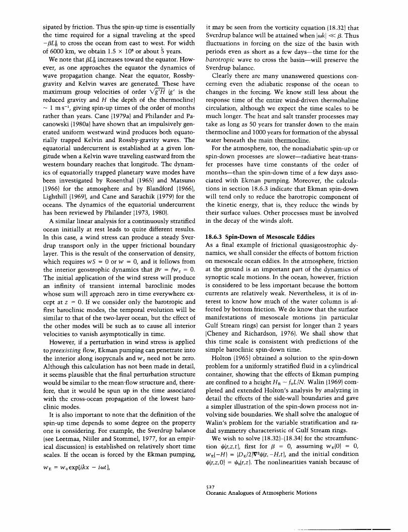
sipated by friction. Thus the spin-up time is essentiallythe time required for a signal traveling at the speed-fILR to cross the ocean from east to west. For widthof 6000 km, we obtain 1.5 x 108 or about 5 years.

We note that fLR increases toward the equator. How-ever, as one approaches the equator the dynamics ofwave propagation change. Near the equator, Rossby-gravity and Kelvin waves are generated. These havemaximum group velocities of order V\ (g' is thereduced gravity and H the depth of the thermocline)

1 m s-1 , giving spin-up times of the order of monthsrather than years. Cane (1979a) and Philander and Pa-canowski (1980a) have shown that an impulsively gen-erated uniform westward wind produces both equato-rially trapped Kelvin and Rossby-gravity waves. Theequatorial undercurrent is established at a given lon-gitude when a Kelvin wave traveling eastward from thewestern boundary reaches that longitude. The dynam-ics of equatorially trapped planetary wave modes havebeen investigated by Rosenthal (1965) and Matsuno(1966) for the atmosphere and by Blandford (1966),Lighthill (1969), and Cane and Sarachik (1979) for theoceans. The dynamics of the equatorial undercurrenthas been reviewed by Philander (1973, 1980).

A similar linear analysis for a continuously stratifiedocean initially at rest leads to quite different results.In this case, a wind stress can produce a steady Sver-drup transport only in the upper frictional boundarylayer. This is the result of the conservation of density,which requires wS = 0 or w = 0, and it follows fromthe interior geostrophic dynamics that fiv = fw = 0.The initial application of the wind stress will producean infinity of transient internal baroclinic modeswhose sum will approach zero in time everywhere ex-cept at z = 0. If we consider only the barotropic andfirst baroclinic modes, the temporal evolution will besimilar to that of the two-layer ocean, but the effect ofthe other modes will be such as to cause all interiorvelocities to vanish asymptotically in time.

However, if a perturbation in wind stress is appliedto preexisting flow, Ekman pumping can penetrate intothe interior along isopycnals and wz need not be zero.Although this calculation has not been made in detail,it seems plausible that the final perturbation structurewould be similar to the mean flow structure and, there-fore, that it would be spun up in the time associatedwith the cross-ocean propagation of the lowest baro-clinic modes.

It is also important to note that the definition of thespin-up time depends to some degree on the propertyone is considering. For example, the Sverdrup balance(see Leetmaa, Niiler and Stommel, 1977, for an empir-ical discussion) is established on relatively short timescales. If the ocean is forced by the Ekman pumping,

WE = WO exp[ikx - iot],

it may be seen from the vorticity equation (18.32) thatSverdrup balance will be attained when Iwokl <<,3. Thusfluctuations in forcing on the size of the basin withperiods even as short as a few days-the time for thebarotropic wave to cross the basin-will preserve theSverdrup balance.

Clearly there are many unanswered questions con-cerning even the adiabatic response of the ocean tochanges in the forcing. We know still less about theresponse time of the entire wind-driven thermohalinecirculation, although we expect the time scales to bemuch longer. The heat and salt transfer processes maytake as long as 50 years for transfer down to the mainthermocline and 1000 years for formation of the abyssalwater beneath the main thermocline.

For the atmosphere, too, the nonadiabatic spin-up orspin-down processes are slower-radiative heat-trans-fer processes have time constants of the order ofmonths-than the spin-down time of a few days asso-ciated with Ekman pumping. Moreover, the calcula-tions in section 18.6.3 indicate that Ekman spin-downwill tend only to reduce the barotropic component ofthe kinetic energy, that is, they reduce the winds bytheir surface values. Other processes must be involvedin the decay of the winds aloft.

18.6.3 Spin-Down of Mesoscale EddiesAs a final example of frictional quasigeostrophic dy-namics, we shall consider the effects of bottom frictionon mesoscale ocean eddies. In the atmosphere, frictionat the ground is an important part of the dynamics ofsynoptic scale motions. In the ocean, however, frictionis considered to be less important because the bottomcurrents are relatively weak. Nevertheless, it is of in-terest to know how much of the water column is af-fected by bottom friction. We do know that the surfacemanifestations of mesoscale motions (in particularGulf Stream rings) can persist for longer than 2 years(Cheney and Richardson, 1976). We shall show thatthis time scale is consistent with predictions of thesimple baroclinic spin-down time.

Holton (1965) obtained a solution to the spin-downproblem for a uniformly stratified fluid in a cylindricalcontainer, showing that the effects of Ekman pumpingare confined to a height HR - foL/IN. Walin (1969) com-pleted and extended Holton's analysis by analyzing indetail the effects of the side-wall boundaries and gavea simpler illustration of the spin-down process not in-volving side boundaries. We shall solve the analogue ofWalin's problem for the variable stratification and ra-dial symmetry characteristic of Gulf Stream rings.

We wish to solve (18.32)-(18.34) for the streamfunc-tion (r,z,t), first for / = 0, assuming WE(O) = 0,WE(-H) = (DE/2)V2q(r, -H,t), and the initial conditionqJ(r,z,O) = tpo(r,z). The nonlinearities vanish because of


____

the radial symmetry. Taking a Fourier-Bessel trans-form of the streamfunction

I(k,z,t) =f rdrJ(rk)ip(r,z,t),

we find

( - k 2) i(kz,t)= =k 2) i(k,z),T1 S Oz 8" ''' \Oz S Oz

z,,k, 0,t) = 0,

,,t(k, -H,t) = k2DfoS(l-H)(k, -H,t).

Solving for we obtain

I(k,z,t = ,o(k,z) - io(k, -H)F(z;k)(1 - e-*'k't),

where F(z;k) satisfies

Oiaa- 1 F = k 2F,

Oz S Oz

Fz(O;k) = 0,

F,(-H;k)= 1,

and the inverse spin-down time is given by

.(k) = -k 2DEfOS(-H)12 Fz( -H;k)

= [-k 2 S(-H)HIF,(-H;k)o]aBT

where rBT = fDE/2H is the inverse barotropic spin-down time. Thus the inverse baroclinic spin-downtime is simply related to sBT by the factor H dividedby the penetration depth.

For large scales, the motion spins down uniformlythroughout the whole column with or - crBT. For smallscales, the spin-down occurs only over a depth HR andis much more rapid. We expect, therefore, that thesmaller scales will disappear from the deep ocean, per-haps leaving a thermocline signal behind, while thelarger scales will decay more slowly but also morecompletely. In figure 18.12, we show the structuresF(z;k) and inverse spin-down times lr(k) for variousscales 1/k. Absolute decay rates depend upon DE-forDE = 20 m, the time scale r- = 89 days, so thateverything happens in a few months.

For application to rings we assume ito(r,-H)-le (- 1 /2)(r2

ll-

) x 10 cms - 1, which gives maximum cur-rents of 10 cm s - at a radius 1. We solve for the netchange in azimuthal velocity qr(r,z,t -+ 0o) - l0or, z) andcontour this change in figure 18.13. It is seen that thechanges in the thermocline and shallow water are neg-ligible so that the persistence of oceanic thermoclineeddies is quite consistent with theoretical expecta-tions.

When the beta effect is included, important differ-ences occur in the spin-down of linear eddies. Thesimplest case to analyze is for weak friction. Then

F (z)

Or%T

10 100 00

I/k (km)

Figure 8.I 2 Decay in currents F as a function of depth fordifferent radial scales k-. Actual change is given by -F(z) xbottom currents. Lower figure shows ratio of decay rate tospin-down rate for a homogeneous fluid as a function of theradial scale.

r (km)100

100

200

(km)200

Figure 8.I3 Decrease in azimuthal velocity due to bottomfriction when initial bottom currents are 10cms- 'r/) xexp[-(r2/112) + ].


_ ___ I _ ____

kJ

there are two time scales-the period and the spin-down time. The Fourier-Bessel component with wave-number k and (initially) vertical normal mode Fn(z)behaves like

(,.k,t) = ,,(k,O)FA(Z)[o (k/(x + Pt + Y2)

x exp[-crBTF(-H)k 2t/(k2 + X2)].

This follows from the fact that when the solution of(18.33) is expanded in powers of period/spin-down time,the lowest order component is just a steadily propa-gating Bessel-function eddy. The next-order componenthas an inhomogeneous boundary condition due to fric-tion and an inhomogeneous forcing of the equations ofmotion due to the slow time dependence. Multiplyingthis first-order equation of motion by F,(z) and depthaveraging shows that the slow time dependence satis-fies a simple exponential decay law (see also Flierl,1978).

One important feature of this solution is the factthat baroclinic modes decay more slowly than baro-tropic modes both because of the increase in X andbecause of the appearance of the factor F2( -H). Thusa first-mode deformation-scale eddy with F,(-H) =-0.6 and k = X has a decay rate of 0.2 RBT. But theimportant feature is that the p-plane eddy, unlike thef-plane eddy, decays completely. The p-effect permitstransmission of energy downward, where it can be dis-sipated by friction. It appears that nonlinearity canimpede this process because it slows down the disper-sion of a ring (McWilliams and Flierl, 1979).

18.7 Nonlinear Motions

In this section, we shall consider mesoscale flows forwhich the advection of relative vorticity or densityanomaly is important. This can occur either in theform of wave-wave interactions or wave-mean flowinteractions. In both cases we are considering motionsin which there are significant nonlinear interactionsamong various scales. This situation is to be contrastedwith that in section 18.5.3, in which the mean flowprovided a variable environment for the waves but waspassive in the sense that there was no exchange ofenergy between the waves and the mean flow.

18.7.1 Baroclinic and Barotropic InstabilitiesThe problem of the instability of large-scale atmos-pheric motions has a long history, going back as alwaysto Helmholtz (1888). The discoveries of the polar frontand the polar-front wave by J. Bjerknes (1919) and J.Bjerknes and H. Solberg (1921, 1922) initiated severalinvestigations of the instability of a polar-front model,notably by H. Solberg (1928) and by N. Kotschin (1932).

These studies were incomplete: Solberg's avoided con-sidering the effects of the frontal intersection withground; Kotschin's considered various possible pertur-bation modes but not that of the all important baro-clinic instability. E. Eliasen (1960) conducted a numer-ical study of a problem similar to Kotschin's, but witha vertical wall. However, the detailed exploration ofKotschin's model, a front between two fluids of differ-ent uniform densities and zonal velocities intersectingupper and lower horizontal boundaries, was left to Or-lanski (1968), who considered all the four different in-stability modes-Helmholtz instability of verticalshear coupled with gravitational stability, Rayleighinstability of horizontal shear, baroclinic instability,and mixed baroclinic-barotropic-Helmholtz instabil-ity. Attempts to explain the long atmospheric wavesobserved in the troposphere were initiated by the workof J. Bjerknes (1937) to which we have already referred.Mathematical theories for the instability of a barocliniczonal current with uniform horizontal temperaturegradients were presented by Chamey (1947), Eady(1949), Fj0rtoft (1950), Kuo (1951), Green (1960), Burger(1962), Stone (1966, 1970) and many others-the prob-lem is still being investigated. The stability of a hori-zontally shearing zonal current in two-dimensionalspherical flow was studied by Kuo (1949). The stabilityof flows with both vertical and horizontal shear wasinvestigated by Stone (1969), McIntyre (1970), Sim-mons (1974), Gent (1974, 1975) and Killworth (1980).The last named is the most comprehensive. Integralconditions for instability in more or less arbitrary zonalflows were developed by analogy with Rayleigh's con-dition for two-dimensional parallel flows by Kuo(1951), Charney and Stem (1962), Pedlosky (1964a,1964b), Bretherton (1966a, 1966b), and others.

On the oceanic side, the onset of meandering of thewestern boundary currents has been dealt with by Or-lanski (1969) and Orlanski and Cox (1973). They con-clude that the meandering of the Gulf Stream betweenMiami and Cape Hatteras can be attributed to baro-clinic instability, a result which seems to be in agree-ment with observations of Webster (1961a). The baro-clinic instability of the free Gulf Stream extensionimplies a northward heat transport by the meandersand cutoff vortices. Evidence for such transports is notconclusive. The discovery of the mid-ocean mesoscaleeddies initiated attempts by Gill, Green, and Simmons(1974) and Robinson and McWilliams (1974) to ascer-tain whether these eddies could be ascribed to baro-clinic instabilities of the mid-ocean mean flows. Theresults have not been encouraging. Studies of the be-havior of numerical ocean models also do not supportthis idea (Harrison and Robinson, 1978). If one merelyconverts available potential energy to kinetic energywhile preserving the total energy density per unit area,the perturbation kinetic energies cannot exceed those


. . . A,

of the mean flow, and are therefore too small by anorder of magnitude. Only ad hoc energy-convergencemechanisms give the right magnitudes.

Most of the studies referred to above have dealt withthe instability of a zonal current with horizontal and/orvertical shear. Realistically, we must also be concernedwith the instability of nonzonal and time-dependentflows, including oceanic gyres, forced and free Rossbywaves and waves over topography. Thus we need toconsider more general basic states.

We begin with the quasi-geostrophic potential vor-ticity equations (18.33)-(18.35). We attempt to find abasic solution i'(x,y,z,t) and investigate the growth ofsmall perturbations i'(x,y,z,t) around this basic state.The most straightforward basic state is a steadily trans-lating (possibly at zero speed) unforced, nondissipativeflow field

(v2 +212)dt V2 + d 1 d = 0,

+ (v -i)V(V2 z S -i, ' =

aiTz l

at + (V - i)V ( - ) ,' = o,

(18.53a)

(18.53b)

z = 0, -H.

If we examine the normal modes '(x,y,z,t) =t'(x',y,z)e0t, we have the eigenvalue equation for thegrowth rate

(V + d Iaz S

+ = (x',y,z), x' = x - t,

which satisfies the equations

V2 + + = P(JI + jy, z)az S az

= -(V - i).V( V z S dz P-

with boundary conditions(18.51)

and the boundary conditions

kzL(x',y,0) = T( + y),

qi(x',y, -H) + foS(-H)b(x' + t,y)

= T(I + Cy). (18.52)

Clearly such a solution is possible only if cb, = 0, thatis, if the basic flow is independent of time or if thezonal variation in topography vanishes-waves cannottranslate over varying topography without changingamplitude or shape. The basic flow is stationary in thex', y, z system and in this system the pseudopotentialvorticity is constant along streamlines.

The derivation of (18.51) and (18.52) may indicatethat the restrictions upon the mean flow are quitesevere-no forcing or dissipation. However, our sub-sequent derivations will require only (18.51) and (18.52)and these can hold in much more general conditions.For example, the standard meteorological problem con-siders the instability of zonal flows forced by heatingand perhaps Reynolds stresses and dissipated by radia-tion and surface Ekman pumping. Since both the meanflow and the potential vorticity are functions only ofy, we can still define potential vorticity and surfacefunctionals from (18.51)-(18.52). As long as the forcingand dissipative processes are not significant in the per-turbation dynamics, the formalism below will apply.(We warn, however, that when there is topography orlateral boundaries, the stability problem for forced anddissipated flow may be quite different.)

The perturbation streamfunction qp' = '(x',y,z,t) sat-isfies

(18.54b)

z = -H.

These equations for the perturbation streamfunctionqi' and the growth rate o- will form the basis for dis-cussion of zonal flow instability and wave instabilitiesbelow.

Integral Theorems The classic example of an integraltheorem is, of course, the Rayleigh theorem (1880).However, there is a slightly more general theorem, dueoriginally to Arnol'd (1965) and applied to quasi-geo-strophic flow by Blumen (1968), which we shall extendhere to the problem of traveling disturbances and/orstationary motion over topography. This theoremstates that the flow is stable if the potential vorticityand buoyancy along the bottom surface increase, andthe buoyancy along the top surface decreases, with in-creasing streamfunction, that is, P' _ 0, T - 0, T -

0 everywhere. To prove this, let us assume that P' > 0,T. < 0, and T > 0 everywhere. (The cases for P' = 0or T = 0 or T = 0 everywhere are readily proved.)First, we form an energy equation by multiplying(18.54a) by -'*, volume integrating, adding the con-jugate equation, integrating by parts, and applying theboundary conditions. We obtain

(o- + C-*) fff Vq.)2 + lq/Iz2

= fff q'J(J + y, '*) + c.c. + ff q;( + y, 0,'*)+ c.c. 1I.


(18.54a)

a-1 = -(v - ).V (- - Tb) ,z = 0,

(18.55)

_r_ �__ � II _ 1_ ---�---1III·_�_·_·II�___I CII--- _- �I �_

Next, we form a normalized enstrophy equation bymultiplying (18.54a) by q'*/P' (recalling that P' # 0)and volume integrating to get

(( + *) fff qp,

= - [ fff q '*J( + ey, qJ') + c.c.]. 18.56)

Applying a similar procedure to the upper and lowerboundary conditions, adding the result to (18.55) and(18.56), gives

(f + ot*) fff I Vq/'I2+ 2+ q'2

V2q, + 3y = P(i + jy).

The substitutions

= toe-vYei(kx-ot)

and

c = o/k

show that P(Z) = BfZ/c. Therefore, when the forcingpropagates eastward, the trapped wave is stable. Unlikeordinary propagating Rossby waves, for which < 0,and which Lorenz (1972) has shown to be unstable,forced waves may be stable. We shall consider topo-graphically forced waves in detail in section 18.7.3.

H 1 2+

8T'S(O)IO + HT;S(-H)l;'(- I = 0. (18.57)

For the choice P' > 0, T < 0, and T > 0 the integrandis positive definite, implying that Re(o-) = 0, that is,that the flow is stable. When P', T, or T are every-where zero, the enstrophy or surface-temperature var-iance equations simply show that q'l or liz4l at 0 or-H = 0, so that the term contributing to (18.55) canbe ignored and therefore will also not enter in (18.57).

This completes the proof of the theorem. From therelation between the potential vorticity and thestreamfunction (in the moving coordinate system) andthe relation between the surface buoyancies and thestreamfunctions at the top and bottom surfaces, wecan tell whether the flow is stable or potentially un-stable. In some problems (cf. Howard, 1964b; Rosen-bluth and Simon, 1964) the necessary criterion for sta-bility has been shown to be sufficient. We should alsomention that the normal-mode assumption is not es-sential, so that the theorem applies to an arbitraryinitial disturbance (Blumen, 1968).

In illustration, we note that the theorem implies thatthe Fofonoff (1954) inertial gyre solution,

P() = a, Ts(t) = Tb*() = O, C = 0,

where a is a positive constant, is stable, as first pointedout by McWilliams (1977). We could find many otherstable gyres by numerical means, including topograph-ical effects, by solving (18.51), (18.52) with arbitraryfunctionals P and Tb constrained only to satisfy theproper derivative conditions. The simplest would be totake

P(,z) = a(z)+ + b(z),

with a(z) > 0 and similar linear functionals for theboundary conditions.

A second example is the flow forced by Gulf Streammeandering described in section 18.5.3. In this case,the potential vorticity equation for the forced wave(the basic state) is

Zonal Flows We now specialize to zonal flows =-fuf(y',z)dy', b = 0. For these, we can readily find P'and Ts,b by taking y derivatives of (18.51) and (18.52):

P' = U( -u a - ),

TS = -ufz/lc - u)lz=,S

Tb = (foSby - uz)/l( - )lz=-H,

where c now is completely arbitrary (i.e., the pertur-bation wave speed will be simply doppler shifted by c).In particular, we can choose so that - has adefinite sign. Therefore we see that the flow will bestable if all the three quantities

0 a 1 u

v -~ Oaz S z '

uJ(O),

foS(-H)b, - z,(-H)

have the same sign. Thus we recover the generalizedRayleigh theorem for quasigeostrophic flows: the flowis stable if

Q- = , - _ + U8(z)Q~ , uz S Oz

+ (f.b- z) 8(z + H) (18.58)

is uniform in sign ( is the Dirac delta function). Moreconventional proofs of this theorem also can be foundin Charney and Stern (1962), Pedlosky (1964a), andBretherton (1966b).

A second standard theorem in shear flow instabilitytheory due to Fj0rtoft (1950) can also be generalized tothe quasi-geostrophic flow problem. If we suppose thatQ, vanishes along some curve in the (y, z) plane andfurthermore that u = uc = constant on this curve, theflow will be stable if Q,( - ru) is negative everywhere.This can be demonstrated by choosing c = uf,. Clearlythe requirement that u = uc at all points where


- - az S az U = 0at s O a q' + J(I,q') + J(I',4) = 0,at

is highly restrictive (though it does occur for uf, = 0 oru, = 0 or u,,, + (010z)(llS)(lOOz)a = Ku).

As a practical application, we remark that the Ray-leigh theorem (18.58) implies that the Eady (1949) prob-lem (S = constant, uz = constant, = 0, uf, = 0) canbe stabilized by a sloping topography such that b, >UfffoSl_H. This slope is steeper than the isopycnal slope,so that the density gradient at the bottom becomesopposite in sign to the gradient at the surface.

A second application is to demonstrate the stabiliz-ing effort of (f, especially for eastward flows. We con-sider zonal currents with a barotropic plus a shearedflow with the structure of the flat-bottom first-baro-clinic mode

U(y,z) = UiBT + UBCF1(Z)

with UBT and UBC constants. (Many currents in theocean do seem to have dominantly first-mode shears.)The Rayleigh criterion becomes

Q = B + F,(z) > 0LR

for all z. This can occur only if

R_= ( Au A rIFI(O) < UBC F,10) + F(-H)I< F1 -H)I

where Au is the change in velocity from bottom to top.Using our N2 profile this implies

-4 cms - < Au < 22 cms - .

We see that eastward currents are considerably morestable than westward flows. Gill, Green and Simmons(1974) report on calculations which show weak growthrates for Afu - -5 cm s-. Observations of actual AU'sare not readily available because the midocean density-field measurements are generally contaminated witheddies. However, it is not unlikely that mid-oceanmean currents away from the "recirculation region" ofWorthington (1976) (see also chapters 1 and 3) aresmaller than this magnitude, so that mid-ocean flowsmay very possibly be stable (see also McWilliams,1975).

This result must be viewed with caution, because itis possible for forced meridional currents to be locallyunstable for any value of the shear. We can see this byconsidering the stability of a mean flow

q, = V(z)x - U(z)y,

where we ignore the dynamics of the mechanism thatsupports the V component of flow on the grounds thatits space and time scales are much larger than those ofthe perturbations we wish to consider. The perturba-tions satisfy

where

U(dZ S av-)X( -a S )y

is now not expressible as P(,z). However, we mayconsider perturbations of the form

q' = F(z) exp[ik(x - ct) + ily]

to find

[(U -c) + 1 (k -k212)F

[ az S 0 ( , )]

Applying the usual Rayleigh theorem shows that theflow will be stable unless - (/1z)(l/S)(OlOz)[ +(l/k)v] changes sign. If V 0, however, a proper choiceof I and k (the direction of the perturbation wave) mayalways be made to ensure satisfying the necessary cri-terion for instability. Thus arguments about the zonalflow stability may not directly apply to the Sverdrupcirculation.

The discussion of baroclinic instability has been ex-tended to finite amplitudes by Lorenz (1962, 1963a)using truncated spectral expansions and by Pedlosky(1970, 1971, 1972, 1976, 1979b), Drazin (1970, 1972),and others using expansion techniques in the vicinityof critical values of the stability parameters. Thus far,the systems dealt with have been more applicable tolaboratory models than the actual atmosphere or ocean.A general review has been given by Hart (1979a), whohimself has contributed by experiment and analysis tothe subject.

18.7.2 Wave-Mean Flow InteractionsThe subject of wave-mean flow interaction in the at-mosphere has been treated extensively in connectionwith the manner in which large-scale waves generatedin the troposphere propagate vertically into the strat-osphere and there interact with the mean flow. Oneexample is the so-called sudden-warming phenome-non, the rapid breakdown of the stratospheric wintercircumpolar cyclone accompanied by large-scale warm-ing. Another example is the so-called quasi-biennialoscillation, which has been explained as a wave-meanflow interaction between vertically propagatingRossby-gravity and Kelvin waves and the zonal flow inthe equatorial stratosphere (Lindzen and Holton, 1968;Holton and Lindzen, 1972). A vivid experimental andtheoretical demonstration of this type of interactionhas been given by Plumb and McEwan (1978).


__ _ _� __ _.__ ___ __

Charney and Drazin (1961) have shown that small-amplitude steady waves in quasi-geostrophic, adi-abatic, inviscid flow cannot interact to second orderwith the zonal flow. If there are no critical surfaces atwhich the zonal flow vanishes and there is no dissi-pation, forcing, or transience, no interaction will takeplace. All are present in the quasi-biennial oscillationand in Plumb and McEwan's model. The result of Char-ney and Drazin was originally derived by straightfor-ward calculation. It may also be inferred from an in-dependent study of energy transfer in stationary wavesby Eliassen and Palm (1960), who derive linear relationsbetween the horizontal Reynolds stress, the horizontaleddy heat flux, and the components of the wave energyflux. These works have been greatly extended by An-drews and McIntyre (1976), Boyd (1976), and Andrewsand McIntyre (1978a,b). McIntyre (1980) reviews thesubject.

There have been several suggestions of oceanic anal-ogies: Pedlosky (1965b) and N. Phillips (1966b) haveargued that westward-propagating Rossby waves cancause acceleration of the western boundary currents.Lighthill (1969) attempted to explain the onset of theSomali Current as due to the interaction of Rossby-gravity waves generated by the monsoon winds in themid-Indian Ocean with the flow in the vicinity of theEast African continent. More recently, experiments ofWhitehead (1975) have shown quite clearly that meanflows may be generated by radiated Rossby waves. Hiswork led Rhines (1977) to a theoretical reconsiderationof the wave-mean flow generation problem not onlywhen the geostrophic contours (the f/H lines whichrepresent the streamlines for free inertial motions) areclosed or periodic but also when the contours are open.Rhines's work is important for understanding large-scale forced motions in oceanic basins.

As an illustration of wave-mean flow interaction inan oceanographic context we shall ask again whetherthe waves produced by Gulf Stream meandering maybe responsible for generating and maintaining the so-called recirculation flow found by Worthington (1976)and others. This flow occurs in a region extending some1000 km south of the stream and contains (accordingto Worthington) a sizable westward transport (108m3 s-'). This problem has been addressed by Rhines(1977), who, however, did not consider generation dueto eastward-moving waves.

We consider the barotropic flow south of the GulfStream forced by the streamfunction qi(x, 0,t) = A cos(kx - cot), as in section 18.5.3, but we now include theeffects of bottom Ekman friction and the second-orderinteraction with the mean zonal flow. The stream-function satisfies

p(x,O,t) = A cos(kx - cot),

-- O, y -c.

The linear solution (assuming Ak3/f3 small) will be

q = Re{A exp[i(kx - cot) + vy]},

V = V'k 2 + f3co1(/o2 + o2BT)- iikoBT/(co 2 + r2T),

if the root with positive real part is chosen to satisfythe radiation condition. The nonlinearly forced stream-function field satisfies

w(t + (aBT) + i a(ia = -2A2v2rvike2Vrf

where v, and vi are the real and imaginary parts of v,respectively. Its solution is

(1) = - A22v k e2V2(TBT

or

A2 Vrk 2v,y= A2vreik

O'BT

This is, of course, just the solution to

(TBTU = Y- (IV 7)

with u' and v' taken from the lowest-order solution.The mean flow is determined by a balance between

friction and Reynolds-stress forcing. The importance ofdissipation becomes clear: without friction, v is eitherpurely real or purely imaginary and iu = 0. With fric-tion, we find that the waves transfer momentum intothe mean flow. Moreover, we can show that the mag-nitude of the flow is not sensitive to the spin-downtime /(rBT, as this time becomes very large.

As OrBT becomes small we find

k2 +i - ioBTk/2o2 k2+ k > o0

o/k < - [3/k2

-i -k2 + BTk/2k2 k

- P/k2 < /k < 0.

The forced mean flow is therefore

= A 2 k2

2c 2

( k-t + GBT) V2P + o(+p = -I(O'V21p)

exp 2 k2+fk , >0,W k

o/k < /k2

exp (JfOBTkY/oJ2 - k - ,

- /k2 < o/k < ,


V =-- .

with amplitude independent of (BT. We can estimatethe westward current speeds by relating the amplitudeA to the excursions of the stream in the y direction:

kd = -A cos(kx - wot) do cos(kx - ot).

The maximum westward currents are -3d2. Rhines(1977) has derived from more general considerationsthe result that mean-flow generation is proportional to/, times the square of the displacement. For typicalexcursions of 100-200 km, mean flows of 10-40 cm s-'can be generated. [We should note that, for this prob-lem, the eastward Stokes drift is given by

A2k (k2 + ) exp(2 k2 + py) ,0- i c+ o

which is larger than the westward Eulerian flow so thatthe particle drift is eastward.]

Observations of Gulf Stream meanders usually in-dicate eastward-moving disturbances; therefore muchof the mean flow will be trapped in a distance one-halfthat shown in figure 18.12. The disturbances that gen-erate propagating waves (-,l3k 2 < o/k < 0) can producemean flows over large north-south distances, but theredoes not seem to be enough amplitude in such disturb-ances. (See, however, the remarks in section 18.8)

This very simple calculation indicates that eddy ra-diation from the meandering Gulf Stream can generatea return flow with speeds comparable to those sug-gested by observations (cf. Worthington, 1976;Wunsch, 1978a; Schmitz, 1977; see also chapter 4). Thepredicted north-south scale of the region is quite small,however, unless there is considerably more energy inwestward-going meanders than has been suggested byHansen (1970) or by Robinson, Luyten, and Fuglister(1974).

There is another form of wave-mean flow interac-tion involving overreflection of waves travelingthrough a variable mean-flow field. Lindzen and Tung(1978) recently have demonstrated that barotropic andbaroclinic instabilities may be explained as overreflec-tion phenomena in which Rossby waves impingingupon a critical surface are reflected with a coefficientof reflection greater than unity. The combination of anoverreflecting region in the mean flow with a reflectingboundary can lead to a growing disturbance in whichthe wave picks up energy at each passage into theoverreflecting region.

This concept may be directly applicable to the prob-lem of reflection of Rossby waves from the westernboundary currents.6 Numerous examples of GulfStream rings interacting with the Gulf Stream withoutbeing absorbed can be found in the data presented byLai and Richardson (1977), and at times they appear toincrease in energy as a result of the interaction (Rich-ardson, Cheney, and Mantini, 1977). We suggest the

possibility that overreflection may be involved in thedynamics of mesoscale eddies near the western bound-ary current. Whether or not this is so remains to beseen.

18.7.3 Wave Instability and Form-Drag InstabilityThe fact that Rossby waves may be unstable was firstshown by Lorenz (1972) for a barotropic atmosphere. Ina more detailed exploration of the problem Gill (1974)observed that there are two distinct mechanisms forthe instability: a resonant triad interaction or a shearinstability of the Rayleigh type. Duffy's (1978) andKim's (1978) baroclinic studies showed that baroclin-icity may also cause instability in large-scale waves.As in the instability of zonal flow, the growing baro-clinic modes have the scale of the radius of deforma-tion. Jones (1978) and Fu and Flierl (1980) have exploredthese ideas further as they apply to the ocean.

Wave and Form-Drag Instabilities Just as a freely prop-agating wave provides variations of potential vorticitywhich may lead to instability, topography may producea forced flow whose variations of potential vorticitymay also cause instability. Topography may be a de-stabilizing influence, either because the forced flow isunstable, just as a free wave, to Rayleigh or resonantinstabilities, or else because the topography itself mayhelp-via the form drag produced by the perturbation-to extract energy from the mean flow. The latter typeof instability was first encountered by Charney andDeVore (1979) in their study of blocking (the persist-ence of anomalously high pressure in certain regionsof the atmosphere) in a barotropic atmosphere. In theirmodel, blocking occurs as an alternative flow equilib-rium corresponding to a given forcing of the zonal flowin the presence of sinusoidal topography. It was foundthat the transition from the normal flow state to theanomalous blocking state takes place via a form-draginstability of an intermediate equilibrium state inwhich the zonal flow is superresonant. In this super-resonant state, a small decrease of the zonal flow am-plifies the forced orographic wave and increases theform drag (mountain torque), which in turn deceleratesthe zonal flow still further. Charney and Straus (1980)extended this study to a two-layer baroclinic atmos-phere. Here again there is a form-drag instabilit. Butwhen there is no lower layer flow, the instability iscatalyzed by the form drag: the perturbation derivesits energy from the available potential energy of theHadley circulation generated by thermal forcing; theform drag merely establishes the necessary phase re-lationships.

The connections between this form-drag instabilityand the more familiar resonant or Rayleigh instabilitieshave not been previously explored. For this purpose,consider the simplest wavelike flow of a homogeneous


·i*

ocean and derive the instability conditions for both afree zonally propagating wave and a topographicallyforced Rossby wave in order to elucidate the similari-ties and differences among the respective instabilitymechanisms. We begin by stating the forms of thepotential vorticity functionals P( + y) and the re-sulting perturbation equations. For the Rossby wave,c = -/k 2 , the potential vorticity functional in equa-tion (18.51) is

P(Z,z) = (lc/)Z = - k2Z

with streamfunction

= A sinkx.

The perturbation equation (18.53a) is particularly sim-ple because P' is now a constant:

(rV2q' + (- y + A sinkx, (V2+ k2)0') = 0, (18.59)

where A is completely arbitrary.For barotropic flow over topography of the form

b = b0 sinkx on the -plane, the basic state potentialvorticity equation

V2j +y + fy bo sinkx = P(i)

has the solution

= -7y + A sinkx, A = ffk2 -B

with the linear potential vorticity functional

P(Z) = - Z - k2Z

Here ku is the wavenumber of the stationary wave (kUmay be less than zero). The perturbation equation

yV2"t' + J [- y + A sinkx,s V + ku)J']

=0 (18.60)

is very similar in form to (18.59) except that k and kuare now independent; however, the amplitude A forthe topographical problem is determined by

fobo/Hk 2 - k

Obviously we need only to solve (18.60) and findcr(13,A,k,ku); we can then identify both the free (ku = k)and forced (ku I k) regimes. In actuality the task iseven simpler since dimensional considerations showthat there are only two parameters, M = Ak3/1, andIx = k,uk, that must be varied while computing thenondimensional growth rate o(lAk2.

First, however, we demonstrate that only the k2 >0 case need be considered, since the flow is stable fork2 < 0. This follows readily from (18.57):

(r + cr*) ff IVIi' 2 -+ IV2qtl2 = 0,

which implies that Rossby waves k2 = k2> 0 and

waves forced by eastward flow may be unstable, whilewaves forced by westward flow k 2 < 0 are definitelystable. Again, as in section 18.7.1 we see that stablewaves are generated when the relative motion of theforced wave with respect to the ambient flow is east-ward. In addition, for eastward flow over topography orwestward-propagating free Rossby waves, a necessarycondition for instability is that the perturbation havecomponents with scales larger than k-I and compo-nents with scales smaller than k- 1. This follows fromFourier analyzing ¢' and substituting in (18.57) to get

ffds Is121i'(s)l2 1 - _2 0,

which implies that 1t'(s)l must be nonzero both forsome values of Isl2 larger than k and some valuessmaller than k.7 This is the perturbation form of Fj0r-toft's (1953) result on energy cascades.

We could readily solve the stability problem (18.60)using the mathematical techniques of Lorenz (1972),Gill (1974), Coaker (1977), or Mied (1978) to investigategrowth rates. Alternatively we could discuss the lim-iting behavior-the Rayleigh limit for M = Ak3/f3 >>1, the resonant interaction limit for M << 1, and theform-drag instability-by separate approximations. Weshall do this for the last-named problem because itrepresents a relatively unfamiliar phenomenon. How-ever, to ascertain most clearly the connections betweenthe various types of behavior, it is most simple toemploy the Fourier expansion

qY = eilo [A0eikox + A-_ei(ko-k)r + Alei(ko+k)x + . .. ]

and truncate to the three indicated terms (cf. Gill,1974). The resulting dispersion relation becomes just

(coK2 + B_)(wK + Bo)(coK2 + B 1)

2A2k 2

- 4 (kU - Ko)[(ku - K2 l)(oK1 + B,)4 \Ilu

+ (k2 - K2)(cK2_l + B 1)] (18.61)

using the notation o = io, K 2 = (k0 + nk) 2 + 12, B, =

,(ko + nk)(k2 - K2,)/k2. For Rossby waves we simplyreplace ku by k.

We have sketched the dependence of -r = a/Ak 2 uponko and 1o for various M and tx values in figure 18.14.When M >> 1, there is a broad area of (ko,lo) space inwhich the growth rates are real. The maximum occursfor ko = 0 (this is really a form of Squire's theorem) and


NORMALIZED GROWTH RATE V/2 + &4)1/2,

au= 0.6

7- '/

p = I.

I,,/

M = O M= I

Figure I8.I4 Growth rate divided by Ak 2 as a function of k0,Io for various ratios of the stationary wavenumber to the top-ographic wavenumber t and wave steepnesses M. The solidlines are the zero contour. The dashed contours, separated bythe interval 0.1, correspond to positive growth rates.

the instability equation is similar to the barotropicinstability equation. As M decreases the instability (&real) becomes restricted more and more to a bandaround the frequency resonance line (see below). Whentu decreases from 1 to a quantity smaller than 1 ( >l3/k2), the point of maximum growth rate for M =

moves to smaller wavenumbers lo. For finite M, thesame thing occurs-the largest growth rate moves to-wards k = 0 = 0 as It decreases. On the other hand,when Ix increases from 1 the forced wave becomesstable for small k0 and 1, even for small M, and thewavenumber for maximum growth migrates to smallerscales.

We are thus led to consider the three limits for(18.61):

Strong waves (A or M large): When A is large, thefrequency co is order A and we can neglect all of theB's to find

AVkl -(k2 - K)[Kl(ku - K2_,) + K2 (k2 - K1)]2 2V KK2 22

Clearly the flow will be unstable for K2 < k < K, K2_1;this will always be possible by proper choice of 10 andko. This is just the Rayleigh instability of the shearflow corresponding to the wave field. The maximumgrowth rate occurs at k0 = 0:

[(-1 +1 = j

0,

(18.62)<_ 1)1/2

/ < J 2 ) However, in the topographic case, A can be large notonly for very strong topography (fobok/H >> ), but alsobecause the zonal flow is nearly critical. In the lattercase u = 1, so that the free and forced wave instabilitiesare indistinguishable. If the flow is not critical, butrather is forced by strong topography, the formulashows the maximum growth rate occurs at k0 - 0,10 -- 0.

Weak waves (A very small or M small): Here thecritical condition is that two of the roots of the left-hand side of (18.61)-for example, -Bo/IK and -B,IK2--coalesce. This resonance condition

Bo/K2 = B,IK2

or

ko(k2 - Ko) (ko + k)(ku - K)k2 K2k 2 K 2kuKo kuK1

permits the order A part of the frequency to be complexsince

K2K2(o + B1o/K)2 Ak 2 (k2 - K)(k2 - K2)4

has a complex root for K2 < k 2 < K2. The growth rateis

All 0okl 1(k2 - K2)(K2 - k2)

2 V KoK,

However, the resonance condition must also hold. Wecan relate this to the more familiar wave-resonanceconditions by defining the intrinsic frequencies of thetwo components of the perturbation and also that ofthe mean flow by

o = - f3kIKo,

= -fi(k + k)/K,

= -k/k = -k/k = -k.

The resonance conditions

(k + k, lo) = (ko,lo) + (k,0),

= &jo + 0

both hold. We show the resonance curves and growthrates for various values of k,lk in figure 18.15.

For large Ix (small mean flow speed), the resonantinteraction (except for large lI) is really a triplet inter-action between the two perturbation waves and thetopography itself (rather than the forced wave). This is,of course, a stable situation. As Ix becomes less than


II - --� ~- �--------·--- Ir�---� - - ___

,u= I

_ L

I. I

-2 -1

p = 0.6

-A5u= 1.4

'STABLEI-

Figure i8.rS Curves above x axis show relation between k0and lo required by resonance condition. Curves below axis areplots of -&, showing the dependence of the growth rate uponk 0.

about 0.9, however, the maximum growth rate againoccurs as ko - 0 and lo -- 0 [o - ( 2ko/I - IL2)112].

Form-drag instability: Thus in either case we are ledto consider what will be shown to be a form-drag in-stability-the nonzero growth rates occurring at smallk 0 and lo-when IL < 0.79. There is some difficulty heresince the origin is a singularity for M finite; this prob-lem would be eliminated in a bounded geometry. Forconvenience, we will take the limits ko -. 0 first andthen 10 -- 0 since this case has a simple physical inter-pretation. Applying these limits to (18.61) gives thefrequency:

(a2 = [ k - k ] + A2k (k2 - k2). (18.63)

The flow is unstable when the right-hand side is neg-ative, which cannot occur for Rossby waves k = k,but may occur for topographic waves when ku < k orU is greater than the critical speed /3/k2. In fact, therange is

3/k2 <U <pk ( [� (f boH ) 2] 3)

(The resonant triad instability for /A < 1 does not appearhere; rather, the limit k - 0- and lo - (-ko)1 2 > 0+

must be used.) So far we have looked at the mathe-matics; let us now discuss the physics of this instabil-ity and also show that the truncation to three terms isvalid.

The form-drag instability involves one componentAo which has very large x and y scales and two com-ponents with the same scale as the topography. Ex-amination of the individual amplitudes shows that

A o - 1/10o, so that Aoeo contributes a term in theperturbation streamfunction which is proportional toy-a modification of the zonal mean flow. This sug-gests an alternative approach, which is to consider thezonal x-averaged momentum equation and the equa-tion for the deviations. We begin with the quasi-geos-trophic equations for a homogeneous fluid,

for = pU ,

fou = -Pr

Ut + (uu)b + (uv)1 - 3yv - fov') =- '

vt + (uv), + ( + yu + fou'l = -P

1ui + v~" -- [(ub)2 + (vb)] = 0,H

and consider the zonally averaged equations

(v) = 0,

(u), + (uv). = fo(V())

(V =H (vb),.

If the topography vanishes at some y far from the regionof interest [following the arguments suggested by Hart(1979b), who showed that the Charney-DeVore trun-cated spectral problem was identical to that of forcedflow over topography varying slowly with y], we canintegrate the last equation to find

fo(U>)t + (V),, = (vb).

The vorticity equation can be used to find the x-de-pendent part of the flow. In particular, if we assumethe y scale is very large, we can drop all y derivativesto get two coupled equations:

(U = Hf (vb),

fv., + (,,)V + B =-- (u)b-.

For the topography b = bsinkx, we have a steadysolution

(u = ,

v = Ak coskx.

The deviations from this state satisfy

(u)t =2 Hb (v , sinkx),

+ V' +,8v' = k Ak - f (u)' coskx

= k fb 3_ (u)' coskx,H ffk2 -


____�

Zl O/k

which may be solved explicitly to give the dispersionrelation (18.63). Here too one sees that it is the couplingbetween the change in the zonal flow induced by thewave drag and the change in the waves due to changesin zonal flow which leads to the instability. If we de-crease the mean flow for a supercritical case (i.e., if wetake (u)' to be negative), we produce low vorticity onthe upwind slopes of the topography and high vorticityon the lee slopes. Associated with this vorticity changeis high pressure on the upslope side of the mountainsand low pressure on the downslope. This pressurepushes eastward on the topography so that the topog-raphy pushes westward on the fluid and decelerates themean flow still further.

Flow in the Presence of Topography The previous sec-tion has described the influence of wavy topographyupon the stability of the flows that go over it. However,there also exists topography that does not alter themean-flow structure, either because the mean currentis parallel to the topographic contours or because thecurrents occur only at levels above the peaks of thetopography. In this section, we shall show that thestability of a parallel mean flow in the presence oftopography can be quite different from that of the iden-tical mean flow in a flat-bottomed ocean. We have beenguided by the result of Charney and Straus (1980), whoshow that the form-drag instability can catalyze therelease of available potential energy in a baroclinicshearing flow that would be stable in the absence oftopography. In their study of multiple equilibria andstability in forced baroclinic flow over topography, theyfound that form-drag instability may occur for weakerthermal driving than conventional baroclinic instabil-ity, and that this type of instability leads to transitionfrom one finite-amplitude, quasi-stationary equilib-rium state to another. Baroclinic and barotropic insta-bilities of the stationary topographically perturbedflows give rise to westward-propagating, vacillatingwave motions with periods of the order of 5 to 15 days.They suggest that the form-drag instability leads totransition from one stationary regime to another andthat the observed westward- and eastward-propagatinglong planetary waves (zonal wavenumbers 1-4) are thepropagating instabilities associated with these station-ary regimes.

The simplest and most obvious example of the des-tabilizing effect of topography is the case of zonal bar-otropic flow with meridionally varying topography.The topography alters the effective value of ji andthereby the growth rates and stability criteria: eventhough the energy source remains the horizontal shear,the topography can alter the possibility of extractingthis energy. In particular, the Chamey-Stem necessarycriterion for instability [that /3 - U,, + (fo/H) b, must

change sign in the domain] suggests that instabilitymay occur for lower values of shear when b, 0. Thenecessary condition may, of course, not be sufficient;in particular, when uf, = 0, the flow will be stable evenif 3 + (fo/H)b, changes sign. However, in the case ofsinusoidal i(y) and b(y), the necessary condition seemsalso to be sufficient (using a simple truncated expan-sion in y), and the topography does destabilize the flow.

DeSzoeke (1975) discussed baroclinic flow over mer-idionally varying topography and found that the topog-raphy destabilizes the flow at some wavenumbers bya resonant instability involving two baroclinic waveswhich happen to travel at the same speed. Similar ef-fects can be identified in the work of Durney (1977).We would like to focus our discussion, however, onthe specific problem of destabilization by form-draginstability of a baroclinic flow which is neutrally stablein the absence of topography.

We shall consider the conventional two-layer modelwhose governing equations (cf. Pedlosky, 1979b) are

( at

x [V/1 - 1 +--- (, - 2) + Y] = 0,

(a at + v2*V)

x [V2qJ2 - 1 +-- (q2 - PI) + Ofy +f (1 + )b] = 0,

where v, and i1, are the velocity and streamfunction inthe upper layer and v2 and iq2 the corresponding quan-tities in the lower layer, 8 is the ratio of the upper tothe lower layer mean depths, and X-1 is the layeredversion of the first baroclinic mode deformation radiusXl = fo (1 + 8)21g(Ap/p)HS. We write the x-averagedequations

at [l UY + I + (f - 2)]

a2 a2 X+ + l 2) = o,

- 2 + - 2 - ']

C02 02 8X2at [ U2 + + -1 2 l )]a+5y2 hxZ(\-y2 2 + = (1 + 8)- H OY2 +2;b,

and the equations for the deviations

(-t lxa-) [V - x( 1p# -/+ [/ +-- 8

(X2 - )]


a�-P �--�---s� � � �_� � _ _ _

+ J [+1 V2*1 - A (X2-

[I+ ]

-"( l~"v + ) = o,

'af + 1 + 8 V q,21- -

+ f (1 + 8)b] 8+,2 -A ] ,42

q,21, V X2 fo(l+a)b

- jy 02. [2v + 1 + 8 + + H

If we now consider y scales that are order 1/A cscales or the deformation scale and expandjO°) + A2Uf" + ":, I(x,y) = 1(°0)(x) + A2 i(1)(

.· (where the topography is assumed to vary x) we find

u)' = U2t,

so that the induced changes in mean flow ar,tropic. This occurs because the form-drag forcinlmean is at much larger scales than the defor:scale. Eliminating the u11) terms at second ord(the two mean flow equations, noting that the Restresses drop out because qi'(0 is independent ofind that the barotropic component of the zonis accelerated or decelerated by the form drag,

a =2 foat H

of weak topography to infinitesimal perturbations evenwhen the flow would be baroclinically stable in theabsence of topography. We can do this by consideringthe stability in the special case Au = 3(1 + 8)/8A2 . Thisis the maximum shear for which the Rayleigh neces-sary criterion for stability in the absence of topography,

(I-128 A)( + AU)-O

is satisfied. Equations (18.14)-(18.16) simplify to theset

0u, f0at H

f the x [+ ( + -a - __-- + )

x,y) + +p ) (1 w = ,nly in

*2xx - f 1 f (1 )ffbb '

e baro- We split the streamfunction into sine and cosine partsLg of the as in section 18.7.3 and solve this system of equations

mation to find the growth rate equationer from / \2

eynolds 4 + k2(k2 + 2)2

f y, weal flow + 42 4 4 88.64 (H 1 +8(k2,18.64} +~ H / I + 8 kk 1 k +

while the deviation fields are given by

+ ((t)+ u) axt) +] 1 +8 ]

+ (0 + 1+- ) 1 , = 0, (18.65)[at+ Ux] [q4- -i + -8 (- 1]+(+ 8X2A) fo (1 + 8)u2b,. (18.66)

Here we have dropped the superscript (0) and intro-duced the notation Au for the time-independent shearacross the interface.

From the equations (18.64)-(18.66) one could derivea single nonlinear governing equation for uff2, and deter-mine the linear instability and finite-amplitude evo-lution of the flow. For our purposes, however, it willbe sufficient to demonstrate that the initial stateu2, = 0, '1 = 0, 02 = 0 can be unstable in the presence

+ 2 (-- kk2 - 8 2 k4- 82 H2 \ 1+ 8) ( 1+8=0. (18.67)

The real solutions to (18.67) for several values offoboX1H are shown in figure 18.16. Notice the insta-bility occurring for topographic scales on the order of70 to 110 km, with growth rates proportional to thetopographic height (for small heights, at least). We havethus demonstrated that the available potential energyin the flow can be tapped by the orographic instabilityeven in situations where normal baroclinic instabilityis unable to extract mean-flow energy. Thus it is pos-sible that mesoscale topography plays a role in cata-lyzing the conversion of mean flow potential to eddyenergy in the oceans.

18.7.4 Multiple EquilibriaWe have already mentioned the work of Charney andDeVore (1979) and Charney and Straus (1980), whohave begun to explore the possibility that the atmos-phere may possess a multiplicity of steady equilibrium


----

a f-plane along a variable coastline (see figure 18.18).Let the latitude of the coastline be h(x) and let -j be thenorth-south distance from the coastline. The potentialvorticity equation becomes

h8-o 8 + q2, + 6I{~ + h)= F(q,).

If we split the streamfunction into an upstream part(x - -, h -- 0) 0(,) and a topographically inducedpart X(x,)) we find

[x - h ,-- + 2 = F(* + 4) -[ ( (x 07,q 49,q2J

50 100(18.68)- ph - ~h2,

150k

-' (km)

Figure 8.I6 Normalized growth rates for a topographicallydestabilized vertical shear flow. The curves are labeled byfoboXIlH values.

states for given external forcing in the presence of top-ographic inhomogeneities. In the case of sinusoidal to-pography in a periodic channel, they have found statesresembling both the "normal" configuration in whichthere is a strong zonal flow and a relatively weak waveperturbation, and the "blocking" configuration inwhich there is a weak zonal flow and a relatively strongwave perturbation. They suggest that the blocking phe-nomenon is an equilibrium state which occurs by atransition via a form-drag instability from the normalto the anomalous blocking configuration. Hart (1979b)has applied similar ideas to laboratory flows and hassucceeded in producing stationary multiple equilibriaexperimentally.

Oceanically, one phenomenon that stands out as apossible example of multiple quasi-stable equilibriumstates is the large meander of the Kuroshio whichsometimes occurs. Figure 18.17 shows the two quasi-stable configurations that are observed. The transitionsbetween these configurations occur relatively rapidly.White and McCreary (1976) have considered a modelfor the meandering process involving flow aroundbumps in the Japanese coastline. Because their discus-sion was in terms of linear dynamics, Solomon (1978)has rightly pointed out that the model must have asmooth transition between the two states as the in-dependent variable (the maximum inlet flow speed)varies. If, however, the phenomenon is nonlinear, cat-astrophic changes in the state of the Kuroshio mayoccur: an infinitely small change in parameters mayproduce a finite change in response, and several stableresponses may be possible for the same set of param-eters.

We propose a simple model of this process consistingof the steady, nonlinear flow of barotropic current on

where

F(lT(7)) = /37 + 2

-- 0 fort7 = 0, 17 -<.(18.69)

When u = - k/I0ri is not constant, equation (18.69)implies that F is a nonlinear functional, so that (18.68)becomes essentially a forced nonlinear oscillator equa-tion; it is well known that such equations may havemultiple stable solutions. We note also a similaritybetween the equations here and the equations for flowof a barotropic fluid over topography. In the derivationbelow we assume that the coastline variations aresmall and occur on scales large compared to the cross-stream scale. We shall show that the nonlinearity playsan important role in determining the amplitude of thenonzonal flow component when the upstream flow isnear the critical speed U,. This speed is defined by thecondition that long waves (x wavelength large com-pared to the width of the current) are stationary. Nearcritical speeds, the amplitude becomes large. The low-est-order dynamic equation only determines the cross-stream wave structure. The first-order equation showsa balance between advection by the mean flow, effectsof the coastline variations, dispersion, and nonlinear-ity.

We shall work with the nondimensional forms of(18.68)-(18.69). Our scaling is guided by the versions+ -2) = -pjh + F' (~) ,

= -ph i - U "u

(18.70)

obtained by linearizing in b and h. We obtain F'(Oi) bydifferentiating (18.69). If h = h coskx, resonance oc-curs when


f ob X

,BHf Hfobo,

0.

\0.1

·� - - - -- -I-� �_� � _ _ � ___

I

Figure 8.I7 Sketch of two equilibrium positions of the Ku-roshio. See Taft (1972) and White and McCreary (1976) fordetailed tracks.

2+ = k2 ,

= O, 71 = 0, -.(18.71)

For forcing on a scale long comnared to the width of

x

the current (l/Oxl << l«/711) we expect that one of theunderlined terms in (18.70) will balance the forcingfrom the side-wall variations -h giving - Uho or4 - h,12, where U is the scale of ui and 1 is the cross-stream scale. When the flow profile is nearly critical

Figure I8.i8 Model for coastline induced meadeviation of the coastline from a latitude circ;h(x); the coordinate q1 is equal to y - h(x). The uis fu(y).

Iur long waves--meanmg mat mie ler-nanu slu ondering. The (18.71) vanishes for some nonzero function 4 whichle is denoted also satisfies the boundary conditions, the long-wave.pstream flow solutions of (18.70) have the two underlined terms

nearly canceling, so that the forcing must be balancedby the ,, term. This gives a scale of 8h - h0L2, whereL is the downstream scale of variation of the topogra-phy.

Therefore, we scale x by L, h by ho, by hoL2, q by1, and u by U in (18.68)-(18.69) to find

02 a ( )2]0712 (ax o)

-h + [F( + ) F)]-yM8 4 h

F (( 71)) = 7 + M,,,

with M = U/(I12, y = hoL4/15, and 8 = 12/L2. If we assumethat the width of the current is small compared to thedownstream scale ( 1) and that the variations incoastline are weak enough so that y s 1, we can sim-plify to


___�___�

(2 a02\ ah + )-+81 aP -2 F (=) h

+ F'(I 2+ 0(82) (18.72)

f = A cosx + (A0 + A2 cos 2x) + 2 A cosnx,n=3

which implies a cubic equation for A:

(1 + )A - 2A3[ + (4 + 1 = 1. (18.76)4-0, -- = 0, -

with

F' (I) -Muv),(18.73)

F" (q3) = [1(1 - Mi.)l,

which are known functions of -q given the specificationof the upstream (x - -) flow u ().

We assume that the flow is nearly critical so thatU = U,(1 + A) where U, is the critical speed (definedexactly below) and therefore M = M,(1 + A). We expand(18.72)-(18.73) assuming A - 8 and MC - 1, y ' 1, andfind to lowest order

02 un - Me10

42 u

(18.74)= 0, =0,-

which defines the eigenvalue MC and thus the criticalspeed Uc given the shape of the upstream flow. The rqstructure of must be an eigenfunction G of (18.74),4 = f(x)G(-q). At next order in A and 8, the solvabilitycondition for (18.72) gives

[f d-GC2(l)] f "(x

-h(x) [f d G(,)] + [If G2,,(,) 1] f(x)

+ - f dq G () - - - (1 -Mc,)] f2(X).This ordinary differential equation for the x structureof the wave f(x) is to be solved for a particular form asA/8 and y vary. For convenience we shall normalize Gand redefine parameters slightly to write

f,,- Af + f 2 = -h(x). (18.75)

The simplest problem to illustrate the characteristicsof (18.75) is the linear case with h(x) = cosx. (Thistopography extends to x = -, which is not reallyconsistent with our original model: however, it doespoint out some of the properties of these nonlinearflows.) The solution to (18.75) with / = 0 is

cosxf +'

showing a resonance at a = -1 (see figure 18.19).For weak nonlinearity (4 small), we can express f as

a Fourier series

(One can show that the higher-order terms will notcontribute, even near resonance.) Figure 18.19 alsoshows the solution of (18.76) for 5 = 0.2. Here weclearly see that there are three equilibrium states fora < - 1.3. The state with intermediate amplitude is un-stable; thus we see that we can have either a largepositive amplitude wave (in phase with topography) ora small negative amplitude wave (out of phase).

This simple model suggests that the Kuroshio mean-der may be a case of multiple states depending on theflow rate at the inlet. Slight decreases in speed maycause a sudden transition to a meander state, withhysteresis effects likely, so that large increases are nec-essary before the Kuroshio would return to its pathcloser to the coast.

The above results merely suggest the possibility ofmultiple equilibria because, to begin with, we haverequired the coastline to have an infinite number ofridges and troughs in order to create the possibility oflinear resonance. As shown in figure 18.10, an infinitenumber of periods may not be necessary, but theremust be at least two ridges and a trough or vice versa.A single coastal ridge (as in the half-wave case) wouldnot be enough to give a maximum response. One must

A

A

A

- ILINEAR

RESONANCE

ILINEAR,SOLUTION

10

.5

0

-5

-10

Figure 8.I9 The wave amplitude as a function of A (propor-tional to the magnitude of the upstream current). Sketchesshow the relationship between the streamlines and the coast-line. Multiple equilibria occur for A < -1.3.


i

'1111� --- ,,,,-�� ___�_ �_�_

ask: Can a single ridge or, in the case of blocking inthe atmosphere, a single mountain range, in an ex-tended domain give rise to multiple equilibria? And isresonance needed?

In problems of nonrotating shallow-water flow overan obstacle, multiple states can exist when the Froudenumber ui/ViH is greater than unity. For certain valuesof the Froude number and the ratio of the obstacleheight to H, two states are found, one correspondingto smooth flow with no upstream disturbance and onecorresponding to a permanent elevation of the free sur-face upstream of the obstacle-created during the ap-proach to equilibrium by a bore traveling upstream(Baines and Davies, 1980). Similar examples of multipleequilibria are also found in transonic compressible flowpast obstacles. Thus we suspect that the upstream flowin our problem cannot be specified arbitrarily but mayvery well be affected by the upstream propagation ofenergy. It may be that, as in the periodic models ofChamey-DeVore and Chamey-Straus, the flow mustbe dealt with as a global or basin-wide unit.

18.7.5 Quasi-Geostrophic TurbulenceWe have considered only wave-wave or wave-meanflow interactions involving a small number of com-ponents. In particular, we have not considered energy-cascade processes involving large numbers of compo-nents and leading ultimately to turbulent dissipation.It was pointed out by Onsager (1949), Lee (1951), Batch-elor (1953a), and especially by Fjortoft (1953) that vor-ticity conservation in two-dimensional flow imposesa strong constraint on scale interactions. Later Charney(1966, 1971a) showed that the conservation of pseu-dopotential vorticity in three-dimensional quasi-geo-strophic flow imposes similar constraints. Such con-straints suggested to Kraichnan (1967) that there maybe an inertial subrange in two-dimensional, homoge-neous, isotropic turbulence in which the energy spec-trum is controlled by uniform transfer of enstrophy(mean-squared vorticity) from large to small scales atscales less than the excitation scale, and by uniformtransfer of energy from small to large scales at scalesgreater than the excitation scale. He predicted a k-3spectral energy density for scalar wavenumber k in theformer range, and a Kolmogorov k-5'3 law in the latterrange. In extending these ideas to three-dimensional,quasigeostrophic turbulence, Chamey (1971a) also ob-tained a k-3 law at the tail of the spectrum and conjec-tured that in this region there would also be equipar-tition between the two components of the kineticenergy and the available potential energy. This conjec-ture has been confirmed by Herring (1980) in a homo-geneous quasi-geostrophic turbulence closure model.

The topic of quasi-geostrophic turbulence has beeninvestigated by a number of oceanographers, notablyRhines (1975) by numerical simulation, and Holloway

and Hendershott (1977) and Salmon (1978) by means ofclosure [see also Herring (1980) and Leith (1971)]. Itmay be that their work is more applicable to the at-mosphere than to ocean basins, where meridionalboundaries play important roles and where statisticalinhomogeneity of excitation cannot be ignored.

The existence of quadratic invariants, energy andenstrophy-mean-squared vorticity in two-dimen-sional or mean-squared pseudopotential vorticity inthree-dimensional quasi-geostrophic flows-permitsapplication of the principles of statistical mechanics.These have been applied by Onsager (1949) and Kraich-nan (1975) to two-dimensional flow, and by Salmon,Holloway, and Hendershott (1976) to a two-layer quasi-geostrophic flow. In the two-dimensional case, the en-ergy in each horizontal mode is L2/(b + aL2), where aand b are constants depending on the total energy andenstrophy. With typical choices of these constants, thelargest scale waves have the most energy. In the two-layer case, the equilibrium spectrum is dominated bythe largest scales, and these motions are barotropic.The available potential-energy spectrum, correspond-ing to the thermocline displacement spectrum, ispeaked near the deformation radius. These spectra rep-resent the effects of the nonlinear terms alone; oneexpects [as Errico (1979) found in studying the partitionof energy between gravity-wave and geostrophic mo-tions] that the spectra which are actually realized in aforced and dissipative system will be determinedlargely by the wavenumber dependence of the forcingand dissipation.

The cornerstone for the theory of quasi-geostrophicturbulence is the conservation (in the inviscid limit) ofthe energy Ifff IV12 + (l/S)lO,/az12 and the enstrophyffff[V2

q + (/z)(ll/S)(O/aOz)] 2. We emphasize the frag-ility of the last principle: enstrophy can increase ordecrease if there are (1) temperature gradients alonghorizontal boundaries, (2) side walls on the domain, or(3) topography.

If we first consider the case when none of theserestrictions obtain-flow in a periodic, flat-bottomeddomain-we can readily argue that the energy will betransferred to large horizontal scales and to more bar-otropic motions by the nonlinear terms. If we expandthe streamfunction in the flat-bottomed normal modesand perform a Fourier transform horizontally,

Y = E F,,(z) ff dki, (k,t)eikx,

we can use the conservation principles

t ff dk (k2 + 2) i.1', = 0,

at ff dk(k + X2)2 lnl2 = 0


(X,, is the reciprocal radius of deformation for the nthbaroclinic mode; see section 18.5.1) in exactly the samemanner as Fjortoft (1953) or Charney (1971a) to showthat the amount of energy with k2 + X2 > K 2 is a smallfraction of the initial energy, if KO is large compared tothe initial mean wavenumber

- ,, ff dk (k2 + X2)1V'2 [(k2 + x2)lg1,2]K =

K,, ff dk[(k2 + X2)ll2]

In essence the nonlinearity does not transfer energy tosmall scales. Another way to show the reverse cascade,is to use Rhines's (1975) argument that the turbulencespreads energy out in wavenumber space

aat , ff dk [(k2 + x2)2 - r] 2[(k2 + x2)1n 12] > 0.

Combining this with the definition of R and using theconservation laws shows that the mean total wave-number must decrease

aK <0.at

Thus energy cascades to larger horizontal and verticalscales, implying an increase in energy for small }X, thatis, a tendency for the motion to become more baro-tropic.

This tendency for the flow to become barotropic inthe absence of topography or side walls has been welldemonstrated through numerical simulation by Rhines(1977). He has also shown that rough topography canhalt this cascade for flows that are not too energetic.The /3-effect slows the cascade when the scale has in-creased so much that the wave steepness M becomesorder one. This could occur while the motions are stillbaroclinic if the initial energy were small compared to32LR.

Rhines (1975) has also argued that side walls can stopthe reverse cascade. This has been demonstrated inlaboratory experiments by Colin de Verdiere (1977). Es-sentially the western boundary serves as a source ofenstrophy and the eastern boundary a sink. This canbe understood-as Pedlosky (1967), in a slightly differ-ent context, has revealed-by considering reflection ofRossby waves from the western boundary. For linearwaves with c = -/(k 2 + 12 + X2), the x componentof the group velocity is negative for k2 < (12 + X2n).Therefore the reflected wave's zonal wavenumber kr =(12 + AX)/k is larger than k. One can readily show thatthe energy fluxes of the incident and reflected waves(cg times the energy density) are equal and opposite,but that the enstrophy flux of the outgoing wave islarger by a factor kr/k than the flux of the incidentwave.

Rhines (1977) has discussed many of the topicsabove, and in particular has demonstrated clearly that

the strong nonlinear interactions involved in geo-strophic turbulence cannot occur unless nonlinearityis much stronger than wave dispersion, that is, unlessthe wave steepness Uk2/fl >> 1. At these scales there issome, but not conclusive, evidence in support of a k- 3

spectrum for the atmosphere (Julian and Clive, 1974).The enstrophy cascade mechanism has not yet beenchecked adequately either by direct measurement orby numerical simulation. It remains possible that theobserved atmospheric spectra can be explained in termsof ordered (periodic) frontal structures, rather than ran-dom cascades of enstrophy, as suggested by Andrewsand Hoskins (1978). They obtain a k-8 '3 dependencywhich is as much in accord with observations as thek- 3 spectrum-or perhaps better. However, the pre-dicted spectra are highly anisotropic, and this does notseem to be in as good agreement with observations orresults from numerical modeling as the predictions ofthe theory of geostrophic turbulence.

So far the data do not exist for a correspondingoceanic check.

18.8 Summary Remarks

Our primary focus has been on oceanic analogues oftransient atmospheric motions of large scale. As prom-ised in the introduction, it has been possible to findformal oceanic analogues for most categories of large-scale atmospheric motions: indeed, it has been almosttrivial to do so. Far more difficult, however, has beento demonstrate the physical reality and importance ofthese analogues. It is only recently, through studies ofthe meanders of the western boundary currents andthrough such concentrated, large-scale observationalprograms as MODE, Polygon, POLYMODE, and theoceanographic component of the GARP Atlantic Trop-ical Experiment (GATE), that some understanding ofthe nature of the transient motions has begun toemerge. Although many of the oceanic analogues wehave dealt with are hypothetical to a greater or lesserdegree, we have chosen them on physical grounds asat least of potential importance. We feel that contrast-ing them with their atmospheric counterparts, withrespect to both their individual properties and theirroles in the generation and maintenance of the large-scale circulation patterns, has been a useful exercise.

In section 18.4, it is shown that the quasi-geos-trophic, 8-plane formalism derived for the atmosphereapplies to oceanic motions whose horizontal scales areon the order of the deformation radius of the first bar-oclinic mode L, that is, the scales corresponding tobaroclinic instability. It is characteristic of these mo-tions that they are dispersive at both small and largeamplitudes. At larger scales the dynamics change: lin-ear free modes may no longer have the same east-westand north-south scales and vertical density advection


_�� I· ____I __ __

becomes an important cause of nonlinearity. For mo-tions with length scales near the "intermediate scale"(La)3 with velocities of order foLla (where a is theradius of the earth), the vertical component of vorticitychanges not only because of p-effects and horizontaladvection but also because of vertical density advectionand variation of the undifferentiated Coriolis parame-ter. Thus both Rossby and Burger terms appear. Foreast-west scales on the order of the intermediate scale(210 km for the ocean and 1500 km for the atmosphere)or larger, dispersion and nonlinearity can balance togive solitary or cnoidal waves. For larger scales, weshow that the evolution is determined by a Korteweg-deVries equation, so that solitons will be the naturalend product of the evolution of an initially isolateddisturbance. Because of the slower dissipation and thelarger scale separation between the intermediate andbasin scales, such waves are more likely to be found inthe ocean than in the atmosphere. These results sug-gest that the larger-scale dynamics of the ocean tran-sients may be dominated by more orderly, phase-coh-erent structures than are predicted by the theory ofgeostrophic turbulence. If this is so, then at scaleslarger than the excitation scale the low-wavenumbercomponents would be more highly correlated than ifthey were due to a random reverse cascade.

The theory of free and forced small-amplitudeRossby waves in the oceans may be transposed almostentirely from the corresponding atmospheric theory.The MODE and Polygon experiments have providedevidence of the importance of Rossby-wave propaga-tion, particularly on time scales greater than a month(McWilliams, 1976). In section 18.5, we present someof this theory in an oceanographic context, paying par-ticular attention to the influence of bottom topographyin altering the propagation of free waves and in gen-erating waves from a mean flow. Rhines's results fora uniformly stratified fluid are extended to arbitrarilystratified flows. The major result, the prediction ofbottom-trapped modes, has been verified from obser-vations at site D (Thompson, 1977) although no obser-vations of the eastward-traveling modes which shouldexist when the topography opposes the p-effect havebeen reported.

The idea of Rossby-wave propagation in a mediumwith a variable (real or imaginary) index of refractionwas first advanced to account for the vertical trappingof shorter waves by upper easterlies and strong wester-lies. We apply these ideas in an oceanographic contextnot only to vertical propagation from the surface orbottom but also to horizontal propagation of wavesgenerated by the meandering of the Gulf Stream. East-ward-propagating meanders produce trapped disturb-ances close to the Gulf Stream, while westward-prop-agating meanders may give a real index of refractionand southward propagation.

In section 18.6, we describe briefly the influence offriction both on the generation of ocean currents bywind and on the decay of individual oceanic eddies.Existing theory is not adequate to account for the spin-up of the real ocean or for the decay of the real atmos-pheric circulation. Interest in the baroclinic spin-downproblem was originally motivated by a desire to un-derstand the long persistence of Gulf Stream rings;however, the axisymmetric models that had previouslybeen employed do not account for the complete decayof a baroclinic eddy. We show that the p-effect permitsvertical propagation of energy and therefore allows forcomplete spin-down.

In the last section, we consider oceanic disturbancesin which advective effects are important-eitherthrough wave-mean flow interaction as in the break-down of an unstable mean flow, through the interac-tion of waves generated elsewhere with the local meanflow, or through wave-wave interactions. The last typeof interaction can occur when the unstable flow isitself a wave or when waves generated in any mannerinteract with one another as in turbulence.

The concept of baroclinic instability was developedto explain the principal traveling waves and vorticesembedded in the atmospheric westerlies; it has beenapplied to the oceans in an effort to account for themeandering of the western boundary currents and theexistence of mid-ocean mesoscale eddies. The mean-dering does seem to be an effect of baroclinic instabil-ity, modified by barotropic effects, but it is highly ques-tionable on theoretical and numerical-modelinggrounds whether the mid-ocean eddies are due to localbaroclinic instabilities. It seems more likely that theseeddies are vortices cast off from, or forced in somemore general fashion by, the meandering westernboundary currents and their extensions.

In our exposition of the baroclinic and barotropicinstability problem, we use the methods of Arnol'd andBlumen to extend the integral theorems of Kuo, Char-ney-Stern, and others to a class of basic flows that neednot be zonal, that may translate with constant speed,and that may be influenced by topography.

The work on wave-mean flow interactions originatedby Eliassen and Palm and Charney and Drazin in anatmospheric context is applied to the problem of therectification of Rossby waves radiated from the westernboundary currents and their extensions. Of particularinterest is the so-called recirculation flow found byWorthington and others south of the Gulf Stream ex-tension. Rhines has attempted to account for this re-circulation as driven by the westward-propagatingRossby waves produced by the meandering. We presenta slight generalization of his work by considering alsothe effects of eastward-traveling meanders. The resultsdo suggest that a relatively strong westward flow, con-fined fairly close to the Gulf Stream, can be produced


·111�

by eastward-propagating wave-mean flow interactionsin the presence of dissipation.

In recent times, the stability analyses for the atmos-phere have been extended to wavy motions in an at-tempt to account for nonlinear cascades of energy inlarge-scale motions. The stability of forced wavy mo-tions has also been studied to account for the transitionfrom one stationary state to another of a forced flowover topography. It has been found from a study ofsimple truncated spectral models that the stationaryflow equilibria produced by the forcing of a zonal flowover topography in a rotating system may be indeter-minate in the sense that for a given forcing, there existsa multiplicity of equilibrium states. This result hasbeen utilized in an attempt to explain the so-calledblocking phenomenon in the atmosphere-the persist-ence of large-amplitude anticyclonic flow anomalies inthe planetary circulation. The existence of multipleequilibria for a given forcing appears to be common; italso occurs for supercritical-Froude-number flow inhydraulics and transonic flow in gas dynamics. A nat-ural oceanic analogue of multiple, quasi-stationaryequilibrium in the atmosphere is the known existenceof two states of flow for the Kuroshio in the vicinityof the Japanese coast. We investigate a simple modelof such a flow and find indeed that two different steadystates may be produced by a given upstream flow as itpasses a wavy boundary. Our model leaves much to bedesired, but it does point a direction for future research.

We find that the transition between one state andanother in topographically forced flows occurs via aform-drag instability in which the perturbed form drag(mountain torque) modifies the mean flow in such away that the perturbation increases in amplitude. Theinstability of a forced topographic wave is thus differ-ent from that of a free wave. The latter instability wasshown by Gill to be basically a Rayleigh-like shearinstability or a resonant-triad wave interaction. Wehave presented the wave-stability analysis for both freeand forced waves in a unified fashion to bring out thesimilarities and differences between the shear, reso-nant, and form-drag instabilities.

The form-drag instabilities producing transitiongrow in place; however, the wavy equilibrium statesthemselves may also exhibit traveling Rayleigh-likeinstabilities. It has been suggested that instabilities ofthis kind account for the observed eastward- and west-ward-propagating very long (zonal wavenumbers 1-4)planetary waves in the atmosphere. One may speculatethat a careful analysis of the topographically inducedmeanders of the western boundary currents in theocean will also reveal such secondary wave instabili-ties. If these are westward propagating, then they couldcontribute to a broader recirculation region.

The final topic is quasi-geostrophic turbulence. Fj0r-toft's prediction that there will be a transfer of energy

from the excitation scale to larger scales in 2-dimen-sional energy-and-enstrophy-conserving flow may beextended to 3-dimensional quasi-geostrophic flows ifthe bottom and top boundaries are flat and isentropic.The theory predicts that the scale will increase verti-cally as well as horizontally, that is, that the flow willbecome increasingly barotropic at large horizontalscales. Rhines has verified this result in a series ofnumerical experiments, and the oceanic observationsof Schmitz (1978) show that the mesoscale eddies tendto be more barotropic the more energetic they are. Thisobservation, while not verifying the inertial theory ofgeostrophic turbulence, is at least consistent with it.As Rhines has shown, the inertial theory applies onlywhen the effects of nonlinearity dominate those oflinear dispersion, that is, when the wave steepnessUk2/,3 is much greater than unity. Thus one expectsthe prediction to be valid only in the energetic parts ofthe ocean. The similarity prediction of a k-3 spectrumat scales smaller than the excitation scale is not incon-sistent with observations in the atmosphere, but thereare as yet no data to test this theory in the ocean. Theeffects of topography, side boundaries, and surface gra-dients of entropy also have not been thoroughly ex-plored.

We have not produced a systematic or comprehen-sive treatment of atmosphere-ocean analogues. Ourexcuse, as we have stated, is that virtually all large-scale atmospheric motions have oceanic counterpartsand there are simply too many of these to discuss. Wehave preferred to deal with analogues for which thereis observational evidence or at least some physical ba-sis for believing they should exist. We have been forcedto speculate, and, as the reader will surely have per-ceived, our own speculations have been guided pri-marily by our own experience and interests.

Appendix: The Quasi-Geostrophic Equations

Here we shall give details of the derivations of thequasi-geostrophic equations. We begin by nondimen-sionalizing the equations of motion (18.22)-(18.27), us-ing the definitions of the geostrophic streamfunctionand the potential buoyancy bp in (18.28) and (18.29).Using the characteristic scales described in the text,we obtain

Du uw tan 0 uv tan28e + &OEXPA -e3 r6 - wcotOw - v_5T r r

r cosO e ('g ctanOe

Dv vw tan A u2 tan2 Oe Dt + x /r r

sin e + tan- sin ,

(18.A1)

(18.A2)


^�_C___I __��__� _� __ _I

Dw U2 + V2 _ oA2E -- EX tan u cot Dt r -Xict

= - t + AS q + b,-EA(b - Aq)(2 - /,cos + tan u+ + + tan v

_v tan20 +o 0+ r2 Wr r2 zz

DwoX2E DW - EXf tan e - Xu cot 0

Dt + bp,

= - + b,(18.A3)

1 D 0 e a1 D sinObp + - Sw - o- w As

sinO Dt e s Oz

+- AE w -- A,(bp - Asq)w = 0.s E)

(18.A4)cA 1 D

- sin D sin (b, - AsqJ) + o{As + AS)wa sinODt

1 D sinOb +-OW (1 -2)Wa sin Dt n + A 1 w

+ edaz S eI +a

+ As)[bp - As(1 + ) ]

+ - A sinO Dt sin = 0,

where

D = ddarcos + tanO Dt +-o 09

+- a + 3tanO a + w za r 0 00 nd

and

r = 1 + X tanOz,

a = 1 + EA(bp - As),

e2 = Cs/C = 1 + O(EA)

are used as abbreviations.The quasi-Boussinesq approximation entails choos-

ing the scale of motion to be small compared to theexternal radius of deformation A << 1. We therefore

drop terms from (18.A1)-(18.A5) which are small inthis sense. The definition of "small" requires somecare because the various Rossby numbers are alsosmall. Thus in equations (18.A1), (18.A2), (18.A4) weshall keep both order 1 and order , E, /3, co terms sothat we may drop only terms of order EA, A, wA. Equa-tions (18.A1) and (18.A2) are changed only slightly: ais replaced by 1. The other equations become

For the ocean, we can further refine these equations bynoting that As is also very small, so that the continuityequation (18.A6}) becomes that of an incompressiblefluid, and the potential buoyancy equation becomessimply

I D sin bp +-w = 0.sin O Dt e

(18.A9)

The hydrostatic approximation applies to a thin layerof fluid: X << 1. This allows us to drop the centrifugalterms involving w, the vertical accelerations, and toreplace r by 1, giving us

DuDu- E/uv tan2 0 - v

= -- e a + tan q- ,

Dv+ E u2 tan2 + U

= - sm ( + / tan 0 ) sin tp,

(18.A10)

(18.All)

cosO + + a + tanO )v-flyan2 (CI w-51- 1 0,

aw- v tan2 0 + c = 0,0z

¢z = bp,

1 a + /tan u + + cos kO f+an o 4 3 hukoo

Ow- ,v tanO + o- z = 0,

where

D 0 + u Dt at e oso (\04 Tt04

(18.A12)

(18.A13)

tan O )v

(18.A14)

rcos0 (d1+ 3 tan 0 )u+ + tan -r cos r

[v tan20 Co + - - r2 w = Ascow,

r r 2 O

+- v +Ptan0 +tanO w

(18.A6) Equations (18.A9)-(18.A14) are the Boussinesq hydro-static equations.

Finally, the quasi-geostrophic -plane approximationassumes that - , - e << 1 and (by necessity) that o


(18.A7)

(18.A8)

____ I_ I

a\TO) V

must also be of this order. We set co = e and expand inpowers of E to find the lowest-order balances

u(O _ &b(O)

O0 '

1 a'q,(O

cose a (9

P - 0O(9z

and the continuity equation

1 au ®'' av ( )

cos 0 a a

which is consistent with the geostrophic equations. Atfirst order we have the momentum equations

u0 1 a (1) tan (o)Dt cosO a cosO M

1DV®0 1 0sD + su (1= - -- sinoDt sin 0 a(

a sin 0 q(0)ocos 0 O

= E (0) -- +-v E

Dt At s cos e a E 00'

from which we form the vorticity equation

St (COSV -U() + e( s + V(1)Dt os0 ' 0¢ i os + V0°

1 a ap(O'' sin e a a(O)0-- sin + sGvcos2 a, ao COS2 e a ao

=-v) - sin avos + tan2v(O) - sin2e aOu(cos a Cos2 c

Combining this with the first-order continuity equa-tion

S sin 9v~ 0

o u' + V(D + sin u + , tan 0O-cos 0 o

- v0"(0tan20 + W =0

(note that for the atmosphere, we would have an ad-ditional term -Asw'° in this equation) leads to thevorticity equation

bD10 1 1 0O<0>+Dcos9 8 4 cosO (o + (o) + (9(9Dt Lc~sO do cose ax 2+-z 3 az $,o

+ 0cose cos

For the atmosphere, the additional term in the conti-nuity equation appears as an extra contribution

s z

in the potential vorticity. Alternatively, the thicknessterm can be written as

0( 1 aa i az a (z) Az ~

for atmospheric quasi-geostrophic motions.

Notes

1. Unfortunately, meteorologists use "mesoscale" very dif-ferently from oceanographers. We shall use mesoscale in theoceanic sense to refer to motions that are dynamically anal-ogous to the "synoptic" scale motions of the atmosphere.

2. Note that the U here is characteristic of the disturbances,not of the mean flow.

3. Some care needs to be used in the cnoidal wave case sincethe mean depth of the fluid becomes H + (1/21rL)fl,~Ldx 7 andthe last term does not vanish. For the figures we have cor-rected for this effect to show c nondimensionalized by f3L,where LR is based on the actual average depth. Thus we haveplotted Cactual = (1 - E(7)l/actua)C as a function of actua =

+ E(n), and also subtracted out the mean from the plots of4'>

. The same process was used for the nonlinear Rossby wavebut had no effect on the dispersion relation.

4. The "anelastic equations" (Batchelor, 1953b; Ogura andCharney, 1962; Ogura and Phillips, 1962) filter only acousticwaves.

5. It is customary to call any quasi-geostrophic wave a Rossbywave.

6. Geisler and Dickinson (1975) studied critical layer absorb-tion in the western boundary current but did not explicitlyinclude a reflected wave. It is also possible that the effects ofthe mechanisms maintaining the western boundary currentare important in the interaction process.

7. It can be shown trivially that there is no nonlinear inter-action in a spectrum of Rossby waves with all componentshaving the same scale (k2 + 2)- 172 (including baroclinic ef-fects).

1 (0) (0) + ( ' = (0)Dt cos0 ) + E

The lowest-order potential-buoyancy equation

DtDt /o, + .w(0) = 0can now be combined with the vorticity equation togive the quasigeostrophic conservation equation:


·4··ll__�-·--a---.·--·-r�__�___ C_�� 1�_� 1�_1�_��__��__·1111II·--· -- -- - I ��

18 oceanic analogues of large-scale atmospheric motions · oceanic analogues of large-scale...

Documents