18 uncertainty in flow gas measurement …€¦ · uncertainty in flow gas measurement systems ......
TRANSCRIPT
__________________________________________________________________________________________________________ 1 Chemical Engineer, Operation and Maintenance Manager - Companhia Maranhense de Gas – Gasmar
18
UNCERTAINTY IN FLOW GAS MEASUREMENT SYSTEMS
WITH ULTRASONIC METERS
Felipe Matuzenetz Marinho1
1 ABSTRACT
Although there are, in many countries, uncertainty ranges acceptable by law and by contracts
signed in fiscal metering of natural gas, in many cases is not defined the methodology for calculation of
this uncertainty. These data, in addition to verify the certainty of the measurement, can be used in
management decisions in equipment and process applications.
This paper applied the methodology shown in GUM (JCGM, 2008), mapping the uncertainties
involved in the metrological process. In the analysis were verified several parameters that are normally
discarded such as the differences between the calibration and process conditions, errors due the heat
transfer between the pipe and the thermowell, variations in atmospheric pressure, and chromatographic
uncertainty. In total, fifty four sources of uncertainty were verified. In addition to these data, were
considered the uncertainties that affect the amount billed, producing a monetary representation of
uncertainty values.
As a case study, was used a custody transfer station in Maranhao / Brazil, with ultrasonic meters
in a flow rate of 2,200,000 Sm³/day, at 32 bar.
The results showed the relevance of factors that generate uncertainty in the final measurement,
generating reliable data to guide management decisions, showing, for example, if is economically feasible
to purchase more expensive and precise equipment, comparing them with the uncertainty values obtained
with these equipment.
2 OBJETIVE
This paper aims to demonstrate the natural gas measurement uncertainty calculations applied at
Companhia Distribuidora de Gás Natural do Maranhão - Gasmar.
The uncertainty calculation in accordance with this document aims to:
• Ensure the measurement reliability of consumed volumes;
• Ensure contractual and regulatory compliance with respect to the criterion of uncertainty
maximum;
• Add value to the product and service provided in volume measurement;
• Ensure traceability and transparency in uncertainty calculation;
• Provide auditable material to give basis for an arbitration in volumes disputes;
• Ensure that invoiced volumes are fair and not unduly benefit any of the parties;
• Give basis for management decisions.
3 INTRODUCTION
The Joint Resolution ANP/INMETRO No. 1, from June 10, 2013, Item 6.4.7 - b, sets the
maximum uncertainty of flow measurement for custody transfer in Brazil at 1.5%. Several other standards
in other countries establish maximum uncertainty parameters. However, the methodology for calculation
of this uncertainty is not defined. This document defines a methodology for calculation of uncertainty and
error in the fiscal measurement based on ISO GUM (JCGM, 2008).
The methodology consists of the individual analysis of each source of uncertainty, combining
uncertainties that interfere in each variable separately and calculating the contribution of each variable on
North Sea Flow Measurement Workshop 2015
Uncertainty in flow gas measurement systems with ultrasonic meters
___________________________________________________________________________________
__________________________________________________________________________________________________________
Page 2/25
the final value. After the calculation of the uncertainty of the measured volume, the uncertainty is then
analyzed over the invoiced amount corresponding to the volume, which includes other sources of
uncertainty, such as tariff calculation.
The methodology was tested and applied in a custody transfer measurement system in Maranhao
/ Brazil using a 10” measurement system, pressure approximately at 32 bar, 40 °C gas temperature,
average flow of 2,200,000 Sm³/day and ultrasonic meter with four pairs of transducers. The straight
segment, as well as the entire system, was designed in accordance with AGA Report No. 9.
In addition to the confirmation of the legal and contractual compliance and measurement
transparency and reliability, these data give basis for management decisions. It can be seen, for example,
if the application of an in line chromatograph at the point of delivery reduces the financial risk of this
application in order to enable the investment cost, just by comparing the difference in billing uncertainty
with and without the chromatograph with the cost of purchasing and installation of the equipment.
4 CALCULATION METHODOLOGY
4.1 Concept and volume uncertainty method
The method demonstrated below is defined in ISO GUM (JCM 2008), applied to the fiscal
measurement of natural gas, in order to quantify the uncertainty arising from this measurement. There
may be variations depending on the measurement system design (equipment, dimensions, etc.) and
processes adopted.
4.1.1 Calculation Method
The calculation of the uncertainty is performed from the partial uncertainties of all variables
that act on the system. To analyze which variables impact the system the definition of the
mathematical model is required. Typical mathematical models in the gas measurement are detailed
in Item 4.2.
After defining the mathematical model, the variables that comprise it and the uncertainties of
each variable are analyzed.
4.1.1.1 Partial Uncertainties
Initially, the individual analysis of each variable that impacts the final result is performed.
A given variable can result in several sources of uncertainty. For example, the variable
temperature may have uncertainty due to repeatability, response time, drift, resolution, etc.
All the variable uncertainties must be identified. The quantification of individual
uncertainties is detailed in Item 4.3.
In order all uncertainties are on the same level of confidence, every uncertainty must be
divided by their respective coverage factor.
4.1.1.2 Combined uncertainty of the variables
After the definition and quantification of the partial uncertainties, the combined uncertainty
is calculated for each variable, algebraically equal to geometric sum of the partial uncertainties
(Equation 1).

North Sea Flow Measurement Workshop 2015
Uncertainty in flow gas measurement systems with ultrasonic meters
___________________________________________________________________________________
__________________________________________________________________________________________________________
Page 3/25
𝑢𝑐𝑗=
𝑘𝑗
2. √∑ 𝑢𝑗𝑖
2
𝑛𝑗
𝑖=1
(1)
Where:
𝑢𝑐𝑗: Combined uncertainty of variable j (same unit of variable j);
𝑘𝑗: Coverage factor of uncertainty 𝑢𝑐𝑗 calculated according to Item 4.1.1.2.1 for a
confidence level of 95,45% (dimensionless);
𝑛𝑗: Number of uncertainties identified from variable j (dimensionless);
𝑢𝑗𝑖: Partial uncertainty i of variable j (same unit of variable j).
4.1.1.2.1 Effective degrees of freedom
Some quantified uncertainties may have been obtained by empirical measurement, in
this case, the number of measurements can affect the results obtained. It is applied then the t-
Student method to correct the measured value to a theoretical condition in which endless
measurements would be performed. This is the case, for example, of the repeatability, which
is obtained by repeated measurement of the same value, checking the variations that occur.
The more measurements are made, the more reliable the result.
Algebraically, this method is reflected in the coverage factor shown in Equation 1,
which is obtained from Table 1 or by the formula shown in
Figure 1 (MS Excel - BR) using the effective degrees of freedom, calculated according
to Equation 2.
𝜈𝑒𝑓𝑓 =𝑢𝑐
4
∑𝑢𝑖
4
𝜈𝑖
𝑁𝑖=1
(2)
Where:
𝜈𝑒𝑓𝑓: Effective degrees of freedom (dimensionless);
𝜈𝑖: Uncertainty degrees of freedom u (dimensionless)i;
𝑢𝑐: Combined uncertainty of the variable analyzed (same unit of the variable analyzed);
𝑢𝑖: Uncertainty i of the variable analyzed (same unit of the variable analyzed);
Figure 1. Calculation of the coverage factor in Excel

North Sea Flow Measurement Workshop 2015
Uncertainty in flow gas measurement systems with ultrasonic meters
___________________________________________________________________________________
__________________________________________________________________________________________________________
Page 4/25
Table 1. Coverage Factor in function of Effective Degree of Freedom and Level of Confidence
Effective Degrees
of Freedom
Level of Confidence
68.27% 90% 95% 95.45% 99% 99.73%
1 1.84 6.31 12.71 13.97 63.66 235.8
2 1.32 2.92 4.3 4.53 9.92 19.21
3 1.2 2.35 3.18 3.31 5.84 9.22
4 1.14 2.13 2.78 2.87 4.6 6.62
5 1.11 2.02 2.57 2.65 4.03 5.51
6 1.09 1.94 2.45 2.52 3.71 4.9
7 1.08 1.89 2.36 2.43 3.5 4.53
8 1.07 1.86 2.31 2.37 3.36 4.28
9 1.06 1.83 2.26 2.32 3.25 4.09
10 1.05 1.81 2.23 2.28 3.17 3.96
11 1.05 1.8 2.2 2.25 3.11 3.85
12 1.04 1.78 2.18 2.23 3.05 3.76
13 1.04 1.77 2.16 2.21 3.01 3.69
14 1.04 1.76 2.14 2.2 2.98 3.64
15 1.03 1.75 2.13 2.18 2.95 3.59
16 1.03 1.75 2.12 2.17 2.92 3.54
17 1.03 1.74 2.11 2.16 2.90 3.51
18 1.03 1.73 2.1 2.15 2.88 3.48
19 1.03 1.73 2.09 2.14 2.86 3.45
20 1.03 1.72 2.09 2.13 2.85 3.42
25 1.02 1.71 2.06 2.11 2.79 3.33
30 1.02 1.7 2.04 2.09 2.75 3.27
35 1.01 1.7 2.03 2.07 2.72 3.23
40 1.01 1.68 2.02 2.06 2.7 3.2
45 1.01 1.68 2.01 2.06 2.69 3.18
50 1.01 1.68 2.01 2.05 2.68 3.16
100 1.005 1.66 1.984 2.025 2.626 3.077
∞ 1 1.645 1.96 2 2.576 3
4.1.2 Sensitivity Coefficient
For the calculation of the global uncertainty, combined to the same analysis variable (in this
case the volume converted to reference conditions), it is necessary to calculate the Sensitivity
Coefficient, which represents the impact the uncertainty of a variable causes in the uncertainty of
the result. When the variables are independent, the sensitivity coefficient is calculated according to
Equation 3. When the sensitivity coefficient of a variable is multiplied by the uncertainty of this
variable, it results in the Contribution of this uncertainty. The geometric sum of the contributions of
each variable generates the overall uncertainty (Taylor series considering that the system is linear),
which multiplied by a coverage factor results in the Expanded Uncertainty (Equation 4).

North Sea Flow Measurement Workshop 2015
Uncertainty in flow gas measurement systems with ultrasonic meters
___________________________________________________________________________________
__________________________________________________________________________________________________________
Page 5/25
𝑐𝑗 =𝜕𝑓
𝜕𝑥𝑗 (3)
𝑈 = 𝑘. √∑ (𝑢𝑐𝑗. 𝑐𝑗)
2𝑁
𝑗=1
(4)
Where:
𝑓: Mathematical model to obtain the results from the variables analyzed;
𝑥𝑗: Variable j;
𝑐𝑗: Sensitivity Coefficient of variable j;
𝑈: Expanded overall uncertainty;
𝑘: Coverage Factor considering infinite degrees of freedom;
𝑁: Number of variables of the mathematical model.
Follow below the sensitivity coefficient of each variable of the mathematical model defined
in Item 4.2.
𝜕𝑉𝑅
𝜕𝑁=
𝑉𝑅
𝑁 ‖
𝜕𝑉𝑅
𝜕𝑃𝐹=
𝑉𝑅
𝑃𝐹 + 𝑃𝐴𝑇𝑀 ‖
𝜕𝑉𝑅
𝜕𝑃𝐴𝑇𝑀=
𝑉𝑅
𝑃𝐹 + 𝑃𝐴𝑇𝑀 ‖
𝜕𝑉𝑅
𝜕𝑇𝐹= −
𝑉𝑅
𝑇𝐹
𝜕𝑉𝑅
𝜕𝑍𝑅=
𝑉𝑅
𝑍𝑅 ‖
𝜕𝑉𝑅
𝜕𝑍𝐹= −
𝑉𝑅
𝑍𝐹 ‖
𝜕𝑉𝑅
𝜕𝑃𝐶𝑆𝐹=
𝑉𝑅
𝑃𝐶𝑆𝐹 (5)
4.2 Definition of the mathematical model
The volume conversion for the base conditions is performed from the Clapeyron equation and it
is shown in Equation 6, considering as negligible the systematic error of the flowmeter (pulse
compensation on the meter).
𝑉𝑅 = 𝑉𝐹 ∙(𝑃𝐹 + 𝑃𝑎𝑡𝑚)
𝑃𝑅∙
𝑇𝑅
𝑇𝐹∙
𝑍𝑅
𝑍𝐹 (6)
Where:
𝑉𝑅 : Volume at base conditions (m³);
𝑉𝐹 : Volume at flow conditions (m³);
𝑃𝐹 : Pressure at flow conditions (Pa);
𝑃𝑎𝑡𝑚 : Local atmospheric pressure (Pa);
𝑃𝑅 : Pressure at base conditions (Pa);
𝑇𝑅 : Temperature at base conditions (K);
𝑇𝐹 : Temperature at flow conditions (K);
𝑍𝑅 : Compressibility at base conditions (dimensionless);
𝑍𝐹 : Compressibility at flow conditions (dimensionless).
To offset the calorific value of the gas, a calorific value factor is included as per Equation 7.

North Sea Flow Measurement Workshop 2015
Uncertainty in flow gas measurement systems with ultrasonic meters
___________________________________________________________________________________
__________________________________________________________________________________________________________
Page 6/25
𝑉𝑅 = 𝑉𝐹 ∙(𝑃𝐹 + 𝑃𝑎𝑡𝑚)
𝑃𝑅∙
𝑇𝑅
𝑇𝐹∙
𝑍𝑅
𝑍𝐹∙
𝑃𝐶𝑆𝐹
𝑃𝐶𝑆𝑅 (7)
Where:
𝑃𝐶𝑆𝑅 : Reference Superior Calorific Value (J/m³);
𝑃𝐶𝑆𝐹 : Superior Calorific Value of the Gas at flow conditions.
Assuming a constant factor K, the volume in flow conditions is detailed depending on the amount
of pulses, according to Equation 8, which also details the calorific value calculated as the method
shown in ISO 6976.
𝑉𝑅 =𝑁
𝐾∙
(𝑃𝐹 + 𝑃𝑎𝑡𝑚)
𝑃𝑅∙
𝑇𝑅
𝑇𝐹∙
𝑍𝑅
𝑍𝐹∙
∑ 𝑥𝑗 ∙ �̃�°𝑗𝑛𝑗=1
𝑍𝑅
𝑃𝐶𝑆𝑅 (8)
Where:
𝑁 : Accumulated amount of pulses (pulses);
𝐾 : Pulses correspondence factor per cubic meter (pulse/m³);
𝑥𝑗 : Mole fraction of the jth component (dimensionless);
�̃�°𝑗 : Ideal calorific value in volumetric base at the base conditions (MJ/m³);
𝑛 : Quantity of natural gas constituent components (dimensionless).
Considering the expansion of the flowmeter body due to pressure and thermal expansion, and
detailing the calculation of the atmospheric pressure based on local altitude, Equation 9 is formed as
follow.
𝑉𝑅 = 𝑉𝑟𝑎𝑤 ∙ 𝐸𝑥𝑝𝐶𝑜𝑟𝑟𝑃 ∙ 𝐸𝑥𝑝𝐶𝑜𝑟𝑟𝑇 ∙
[𝑃𝐹 + 𝑃0 ∙ (1 +𝑎 ∙ ℎ
𝑇0)
−𝑀∙𝑔𝑎∙𝑅
]
𝑃𝑅∙
𝑇𝑅
𝑇𝐹∙
𝑍𝑅
𝑍𝐹∙
∑ 𝑥𝑗 ∙ �̃�°𝑗𝑛𝑗=1
𝑃𝐶𝑆𝑅 (9)
Where:
𝑉𝑟𝑎𝑤 : Raw volume measured by flowmeter (m³);
𝐸𝑥𝑝𝐶𝑜𝑟𝑟𝑃 : Correction factor of the flowmeter expansion due to pressure (dimensionless);
𝐸𝑥𝑝𝐶𝑜𝑟𝑟𝑇 : Correction factor of the flowmeter expansion due to thermal expansion
(dimensionless);
𝑃0 : Atmospheric pressure at reference location (Pa);
𝑎 : Rate of temperature variation in relation to altitude (K/m);
ℎ : Altitude in relation to atmospheric base point (m);
𝑇0 : Temperature at atmospheric base point (K);
𝑀 : Air mole mass (kg/m³);
𝑔 : Local gravity (m/s²);
𝑅 : Universal gas constant (J/mol.K).
Details of the correction factors of the flowmeter expansion due to pressure and temperature is
shown in Equation 10.

North Sea Flow Measurement Workshop 2015
Uncertainty in flow gas measurement systems with ultrasonic meters
___________________________________________________________________________________
__________________________________________________________________________________________________________
Page 7/25
𝐸𝑥𝑝𝐶𝑜𝑟𝑟𝑃 ∙ 𝐸𝑥𝑝𝐶𝑜𝑟𝑟𝑇 = 1 + [3 ∙ ([𝐷𝑜𝑢𝑡
2 ∙ (1 + 𝜐)] + [𝐷𝑖𝑛2 ∙ (1 − 2 ∙ 𝜐)]
𝐸 ∙ (𝐷𝑜𝑢𝑡2 − 𝐷𝑖𝑛
2 )) ∙ (𝑃𝐹 + 𝑃𝑎𝑡𝑚 − 𝑃𝑅)] (10)
Where:
𝐷𝑜𝑢𝑡 : Outer diameter of the piping or flowmeter (m);
𝐷𝑖𝑛 : Inner diameter of piping or flowmeter (m);
𝜐 : Poisson Coefficient (dimensionless);
𝐸 : Young Module (MPaa).
To simplify the analysis and calculation process of the uncertainty of the parameters analyzed, it
is used the basic model defined in Equation 7, details shown in Equations 8, 9 and 10 are calculated
separately.
4.3 Uncertainty Sources
To check the uncertainties in the reference volume, the individual variables are analyzed, which
are shown below.
4.3.1 Uncertainties related to the quantity of accumulated pulses (N)
4.3.1.1 Reading Resolutions
The transmission of flow by pulses has the range uncertainty of a pulse due to the
resolution. The higher the frequency of pulses per cubic meter is, the lower the impact of this
uncertainty on the volume.
4.3.1.2 Loss of Pulse
Accumulated pulses differences between the generated by the flow meter and the received
by flow computer accumulator may eventually occur. These differences may happen for various
reasons, such as the interferences in the inductive environment, contact with corrosion, and
incompatible impedance. The estimation of loss of pulse is performed based on the analysis of
the history between the flow meter accumulator and the flow computer accumulator.
4.3.1.3 Uncertainty Inherited From the Calibration Laboratory
The analyzed measurement system has a calibration curve correction in the flow meter.
The values used in the curve correction are subject to the calibration laboratory uncertainties and
should be taken into consideration in the analysis. It is obtained with the multiplication of the
uncertainty informed in the calibration certificate of the flowmeter (comprising all the
uncertainties of the laboratory, such as the ones inherited from patterns, repeatability, etc.) by the
calibrated flow range and the K factor.
4.3.1.4 Drift of Flowmeter
Every measurement instrument has a tendency to increase the uncertainty with the use of
the equipment. This can be observed in the As Found calibration report. In order to estimate how
much the uncertainty increases during the inter calibration period, a linear regression is made
considering the last adjustment period and the geometric sum of the repeatability and the
systematic error. The resulting equation is applied to estimate the increase of uncertainty for the
analyzed period considering the last calibration performed in the flowmeter.
North Sea Flow Measurement Workshop 2015
Uncertainty in flow gas measurement systems with ultrasonic meters
___________________________________________________________________________________
__________________________________________________________________________________________________________
Page 8/25
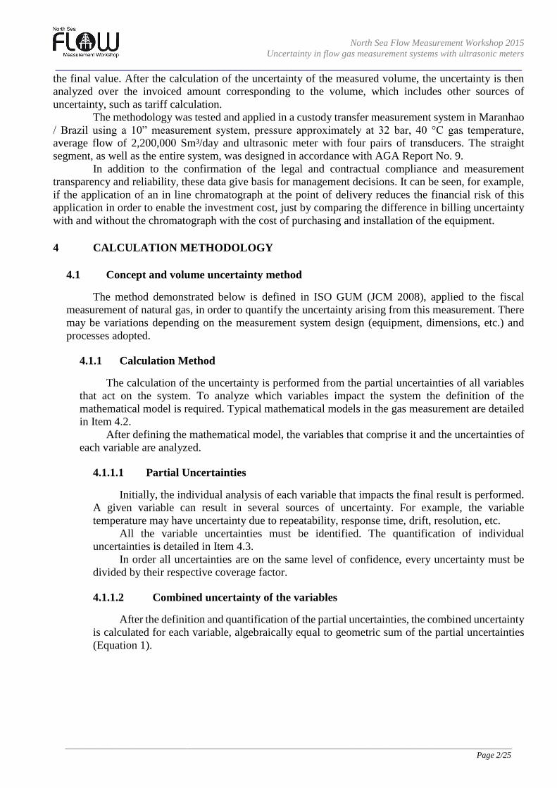
4.3.1.5 Expansion by Pressure
The uncertainty related to the increase in distance between the ultrasonic transducers due
to the expansion by pressure. This is obtained with the individual analysis of the uncertainties
that compose the equation of expansion by pressure, as seen in Equation 11.
𝐸𝑥𝑝𝐶𝑜𝑟𝑟𝑃 = 1 + 3 ∙[𝐷𝑜𝑢𝑡
2 ∙ (1 + 𝜐)] + [𝐷𝑖𝑛2 ∙ (1 − 2 ∙ 𝜐)]
𝐸 ∙ (𝐷𝑜𝑢𝑡2 − 𝐷𝑖𝑛
2 )∙ (𝑃𝐹 + 𝑃𝑎𝑡𝑚 − 𝑃𝑅) (11)
In this case study, the uncertainties that came from the measurements of the flowmeter’s
inner and outer diameter, the Poisson coefficient, and the Young Module, were not taken into
account, considering only the uncertainties that came from the pressure and atmospheric pressure
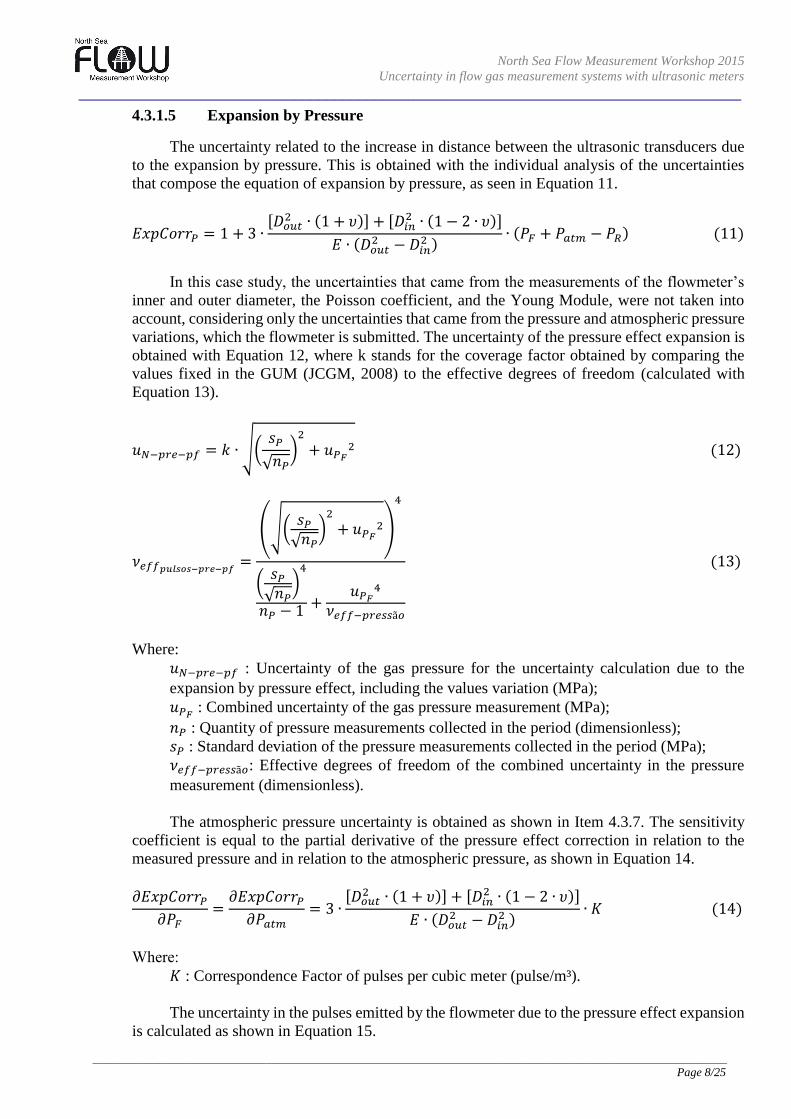
variations, which the flowmeter is submitted. The uncertainty of the pressure effect expansion is
obtained with Equation 12, where k stands for the coverage factor obtained by comparing the
values fixed in the GUM (JCGM, 2008) to the effective degrees of freedom (calculated with
Equation 13).
𝑢𝑁−𝑝𝑟𝑒−𝑝𝑓 = 𝑘 ∙ √(𝑠𝑃
√𝑛𝑃
)2
+ 𝑢𝑃𝐹2 (12)
𝜈𝑒𝑓𝑓𝑝𝑢𝑙𝑠𝑜𝑠−𝑝𝑟𝑒−𝑝𝑓=
(√(𝑠𝑃
√𝑛𝑃)
2
+ 𝑢𝑃𝐹2)
4
(𝑠𝑃
√𝑛𝑃)
4
𝑛𝑃 − 1 +𝑢𝑃𝐹
4
𝜈𝑒𝑓𝑓−𝑝𝑟𝑒𝑠𝑠ã𝑜
(13)
Where:
𝑢𝑁−𝑝𝑟𝑒−𝑝𝑓 : Uncertainty of the gas pressure for the uncertainty calculation due to the
expansion by pressure effect, including the values variation (MPa);
𝑢𝑃𝐹 : Combined uncertainty of the gas pressure measurement (MPa);
𝑛𝑃 : Quantity of pressure measurements collected in the period (dimensionless);
𝑠𝑃 : Standard deviation of the pressure measurements collected in the period (MPa);
𝜈𝑒𝑓𝑓−𝑝𝑟𝑒𝑠𝑠ã𝑜: Effective degrees of freedom of the combined uncertainty in the pressure
measurement (dimensionless).
The atmospheric pressure uncertainty is obtained as shown in Item 4.3.7. The sensitivity
coefficient is equal to the partial derivative of the pressure effect correction in relation to the
measured pressure and in relation to the atmospheric pressure, as shown in Equation 14.
𝜕𝐸𝑥𝑝𝐶𝑜𝑟𝑟𝑃
𝜕𝑃𝐹=
𝜕𝐸𝑥𝑝𝐶𝑜𝑟𝑟𝑃
𝜕𝑃𝑎𝑡𝑚= 3 ∙
[𝐷𝑜𝑢𝑡2 ∙ (1 + 𝜐)] + [𝐷𝑖𝑛
2 ∙ (1 − 2 ∙ 𝜐)]
𝐸 ∙ (𝐷𝑜𝑢𝑡2 − 𝐷𝑖𝑛
2 )∙ 𝐾 (14)
Where:
𝐾 : Correspondence Factor of pulses per cubic meter (pulse/m³).
The uncertainty in the pulses emitted by the flowmeter due to the pressure effect expansion
is calculated as shown in Equation 15.
North Sea Flow Measurement Workshop 2015
Uncertainty in flow gas measurement systems with ultrasonic meters
___________________________________________________________________________________
__________________________________________________________________________________________________________
Page 9/25
𝑢𝑁−𝑝𝑟𝑒 =
√(𝜕𝐸𝑥𝑝𝐶𝑜𝑟𝑟𝑃
𝜕𝑃𝐹∙ 𝑢𝑁−𝑝𝑟𝑒−𝑝𝑓)
2
+ (𝜕𝐸𝑥𝑝𝐶𝑜𝑟𝑟𝑃
𝜕𝑃𝑎𝑡𝑚∙ 𝑢𝑃𝑎𝑡𝑚
∙ 𝑘𝑃𝑎𝑡𝑚)
2
2 (15)
Where:
𝑢𝑁−𝑝𝑟𝑒 : Uncertainty of the number of pulses due to the pressure effect expansion (pulses);
𝑢𝑃𝑎𝑡𝑚 : Uncertainty of the atmospheric pressure (MPa).
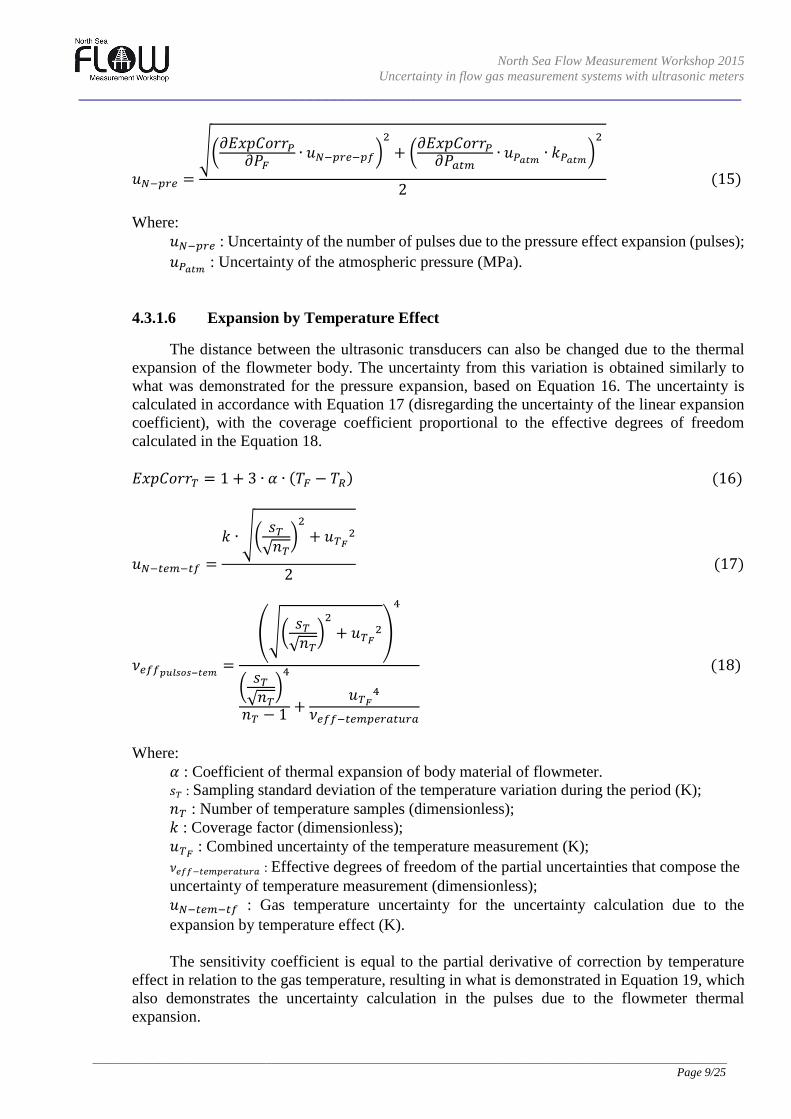
4.3.1.6 Expansion by Temperature Effect
The distance between the ultrasonic transducers can also be changed due to the thermal
expansion of the flowmeter body. The uncertainty from this variation is obtained similarly to
what was demonstrated for the pressure expansion, based on Equation 16. The uncertainty is
calculated in accordance with Equation 17 (disregarding the uncertainty of the linear expansion
coefficient), with the coverage coefficient proportional to the effective degrees of freedom
calculated in the Equation 18.
𝐸𝑥𝑝𝐶𝑜𝑟𝑟𝑇 = 1 + 3 ∙ 𝛼 ∙ (𝑇𝐹 − 𝑇𝑅) (16)
𝑢𝑁−𝑡𝑒𝑚−𝑡𝑓 =
𝑘 ∙ √(𝑠𝑇
√𝑛𝑇)
2
+ 𝑢𝑇𝐹2
2 (17)
𝜈𝑒𝑓𝑓𝑝𝑢𝑙𝑠𝑜𝑠−𝑡𝑒𝑚=
(√(𝑠𝑇
√𝑛𝑇)
2
+ 𝑢𝑇𝐹2)
4
(𝑠𝑇
√𝑛𝑇)
4
𝑛𝑇 − 1 +𝑢𝑇𝐹
4
𝜈𝑒𝑓𝑓−𝑡𝑒𝑚𝑝𝑒𝑟𝑎𝑡𝑢𝑟𝑎
(18)
Where:
𝛼 : Coefficient of thermal expansion of body material of flowmeter.
𝑠𝑇 : Sampling standard deviation of the temperature variation during the period (K);
𝑛𝑇 : Number of temperature samples (dimensionless);
𝑘 : Coverage factor (dimensionless);
𝑢𝑇𝐹 : Combined uncertainty of the temperature measurement (K);
𝜈𝑒𝑓𝑓−𝑡𝑒𝑚𝑝𝑒𝑟𝑎𝑡𝑢𝑟𝑎 : Effective degrees of freedom of the partial uncertainties that compose the
uncertainty of temperature measurement (dimensionless);
𝑢𝑁−𝑡𝑒𝑚−𝑡𝑓 : Gas temperature uncertainty for the uncertainty calculation due to the
expansion by temperature effect (K).
The sensitivity coefficient is equal to the partial derivative of correction by temperature
effect in relation to the gas temperature, resulting in what is demonstrated in Equation 19, which
also demonstrates the uncertainty calculation in the pulses due to the flowmeter thermal
expansion.

North Sea Flow Measurement Workshop 2015
Uncertainty in flow gas measurement systems with ultrasonic meters
___________________________________________________________________________________
__________________________________________________________________________________________________________
Page 10/25
(𝜕𝐸𝑥𝑝𝐶𝑜𝑟𝑟𝑇
𝜕𝑇𝐹= 3 ∙ 𝛼 ∙ 𝐾) → 𝑢𝑁−𝑡𝑒𝑚 = 𝑢𝑁−𝑡𝑒𝑚−𝑡𝑓 ∙
𝜕𝐸𝑥𝑝𝐶𝑜𝑟𝑟𝑇
𝜕𝑇𝐹 (19)
Where:
𝐾 : Correspondence Factor of pulses per cubic meter (pulse/m³);
𝑢𝑁−𝑡𝑒𝑚 : Uncertainty of the number of pulses due to the expansion by temperature effect
(pulses).
4.3.2 Uncertainties Related to the Gas Pressure’s Measurement (PF)
4.3.2.1 Repeatability
Uncertainty related to the capacity of the instrument to show the same measurement in the
same point repeatedly. It is estimated during the calibration of the pressure transmitter and is
numerically equal to the greatest calculated value of the division between the standard deviation
and the square root of the number of measurements, for each measurement point during the
calibration, and multiplied by a coverage factor that equals two, as per demonstrated in Equation
20.
𝑢𝑃𝐹−𝑟𝑒𝑝 =𝑠
√𝑛=
√∑ (𝑥𝑖 −∑ 𝑥𝑗
𝑛𝑗=1
𝑛 )
2
𝑛𝑖=1
𝑛 − 1
√𝑛 (20)
Where:
𝑢𝑃𝐹−𝑟𝑒𝑝 : Uncertainty related to the repeatability of the instrument (Pa);
𝑠 : Standard Deviation of Measurements (Pa);
𝑛 : Number of Measurements (dimensionless);
𝑥𝑖 , 𝑥𝑗: Pressure Measurement (Pa).
4.3.2.2 Hysteresis
The hysteresis is related to the capacity of the instrument to show the same measurement
at the same point in ascending and descending measurements. It is estimated during the
calibration of the pressure transmitter and is numerically equal to the greatest calculated value
found in the module of the average difference between the ascending and descending calibration
measurements, as per Equation 21.
𝑢𝑃𝐹−ℎ𝑖𝑠 = |∑𝑥𝑎
𝑛
𝑛2
𝑎=1
− ∑𝑥𝑑
𝑛
𝑛2
𝑑=1
| (21)
Where:
𝑢𝑃𝐹−ℎ𝑖𝑠 : Uncertainty due to hysteresis of the pressure meter instrument (Pa);
𝑛 : Number of measurements (dimensionless);
𝑥𝑎 : Ascending pressure measurement (Pa);
𝑥𝑑 : Descending pressure measurement (Pa).
North Sea Flow Measurement Workshop 2015
Uncertainty in flow gas measurement systems with ultrasonic meters
___________________________________________________________________________________
__________________________________________________________________________________________________________
Page 11/25
4.3.2.3 Standard Instrument Resolution
The resolution of the standard instrument used in the calibration is also a source of
uncertainty and is obtained in the certificate of calibration of the standard instrument.
4.3.2.4 Uncertainty inherited from calibration standard instrument
Like the resolution, the uncertainty inherited from the standard instrument is also
considered and obtained from the certificate of calibration of the standard instrument multiplying
by the calibrated amplitude of the standard instrument.
4.3.2.5 Instrument Resolution
The instrument resolution represents the truncation of the measured value. In the analyzed
system, the signal transmission of the instrument is made via the 4-20mA communication and
the resolution is limited by the D/A converter, which is obtained from the transmitter manual,
multiplying the value by the signal transmission amplitude.
4.3.2.6 Uncertainty of the 4-20mA current meter
The uncertainty related to the 4-20mA current meter instrument used in the calibration. It
is obtained in the certificate of calibration of the current meter. It is algebraically obtained
multiplying the uncertainty in the certificate of calibration of the current meter by the amplitude
of the signal transmission (in pressure unit) and divided by the amplitude signal transmission in
current (with the 4-20mA, the amplitude would be 16mA), as shown in Equation 22.
𝑢𝑃𝐹−𝑚𝑐𝑐 =𝑢𝑐𝑜𝑟𝑟𝑒𝑛𝑡𝑒−𝑚𝑐𝑐 ∙ 𝑎𝑝
𝑎𝑐 (22)
Where:
𝑢𝑃𝐹−𝑚𝑐𝑐 : Uncertainty inherited from 4-20mA signal meter used in calibration (Pa);
𝑢𝑐𝑜𝑟𝑟𝑒𝑛𝑡𝑒−𝑚𝑐𝑐 : Uncertainty of 4-20mA signal meter used in calibration (mA);
𝑎𝑝 : Transmitter measurement amplitude (Pa);
𝑎𝑐 : Signal transmitter amplitude (for transmission of 4-20mA ac=16mA) (mA).
4.3.2.7 Signal Generator Uncertainty in Loop Test
In the analyzed system, the instruments are removed from installation site for calibration
and the communication mesh is verified separately. The values obtained are compensated in the
calibration values. A signal generator is used for the test of the communication mesh. The signal
generator uncertainty multiplied by the signal transmission amplitude (in pressure unit) divided
by the signal transmission amplitude in current units is the value considered as uncertainty due
to the use of this equipment (similar to what was demonstrated in Equation 18).
4.3.2.8 Pressure Variations
The flow computer has a calculation cycle that performs the data reading of the instruments
and calculates the volume at base conditions. If there are pressure variations in time shorter than
the flow computer sampling, these variations will not be recorded. The shorter the sampling time
is, the lower the uncertainty due to the pressure in the sampling intervals. The uncertainty value
is the standard deviation of the variations in time of the flow computer cycle divided by the
square root of the quantity of analyzed variations.

North Sea Flow Measurement Workshop 2015
Uncertainty in flow gas measurement systems with ultrasonic meters
___________________________________________________________________________________
__________________________________________________________________________________________________________
Page 12/25
4.3.2.9 Environment Temperature Effect
The electronic components of the transmitters go through minor changes due to the
temperature. These changes can be adjusted in the calibration, but some differences may happen
when the temperature in the calibration is different from the temperature in the process. The
closest the process temperature is to the temperature in the calibration, the lower this uncertainty
will be. Each manufacturer has a calculation method to achieve this uncertainty, which can be
found in the manual of the instrument. For the Rosemount transmitter 3051, the uncertainty due
to the effect of the environment temperature is calculated according to Equation 23.
𝑢𝑃𝐹−𝑒𝑡𝑎 =(25 ∙ 𝐿𝑆𝐹 + 125 ∙ 𝑎) ∙ 10−5
28∙ |𝑇𝑎𝑚𝑏−𝑝𝑟𝑜 − 𝑇𝑎𝑚𝑏−𝑐𝑎𝑙| (23)
Where:
𝑢𝑃𝐹−𝑒𝑡𝑎 : Uncertainty due to the environment temperature variation (Pa);
𝐿𝑆𝐹 : Upper range limit of transmitter (bar);
𝑎 : Calibration amplitude of transmitter (bar);
𝑇𝑎𝑚𝑏−𝑝𝑟𝑜 : Average environment temperature at the installation site (°C);
𝑇𝑎𝑚𝑏−𝑐𝑎𝑙 : Average environment temperature during the calibration (°C).
4.3.2.10 Pressure Meter Drift
Similar to what was demonstrated in Item 4.3.1.4, the pressure meter is subject to the drift
effect, and this uncertainty is calculated by the linear regression considering the last adjustment
period and the geometric sum of the repeatability, the hysteresis, and the systematic error. The
resulting equation is used to estimate the increase in uncertainty for the analyzed period
considering the last calibration performed in the instrument.
4.3.2.11 Assembling position of Transmitter
The assembling position (horizontal, vertical, or inclined) can interfere the pressure
measurement. This uncertainty can be eliminated in the calibration adjustment. In the analyzed
measurement system, the calibration is performed in the same vertical inclination of the
installation position. However, once the instrument is moved during the calibration, there might
be a slight difference between the calibration measurement and the installed instrument
measurement. The manufacturer informs this uncertainty estimative.
4.3.2.12 Electric Variation
Voltage variations of the instruments might propagate in signal transmission and result in
interferences in measurement. The uncertainty value depends on the instrument voltage and is
informed by the manufacturer.
4.3.3 Uncertainties related to flow temperature (TF)
4.3.3.1 Repeatability
Such as the calculation for the pressure transmitter (Equation 20), the repeatability is also
taken into consideration for the temperature measurement.

North Sea Flow Measurement Workshop 2015
Uncertainty in flow gas measurement systems with ultrasonic meters
___________________________________________________________________________________
__________________________________________________________________________________________________________
Page 13/25
4.3.3.2 Uncertainty inherited from the standard instrument
The uncertainty of the standard instrument used in the calibration of temperature instrument
constitutes the variable uncertainty calculation and must be in absolute values of temperature.
4.3.3.3 Resolution of Calibration Standard Instrument
The standard temperature instrument used in the calibration should be considered
(instrument of measurement or indication of temperature bath).
4.3.3.4 Axial Homogeneity of the temperature bath
There might be differences in the measurement of the calibration bath depending of the
vertical insertion position of the sensor. These differences create errors in the calibration process.
The estimate of the calibration bath homogeneity is achieved with tests in various conditions,
and is informed by the manual of manufacturer equipment.
4.3.3.5 4.3.3.5 Radial Homogeneity of temperature bath
Similar to the axial homogeneity, there is also an uncertainty due to the insertion horizontal
position of the sensor. This value can also be found in the manual of the equipment.
4.3.3.6 Uncertainty of the 4-20mA meter
Similar to the calculation of the pressure instrument, the 4-20mA signal meter equipment
is considered in the temperature uncertainty.
4.3.3.7 Precision of the Signal Generator in Loop Test
Similar to the calculation of pressure meter instrument, when the Loop Test is used to
compensate the error in the communication mesh, the uncertainty of the signal generator is
considered.
4.3.3.8 Thermal Transfer of the Thermowell
When a thermowell is used in the temperature measurement, there might be thermal
transfers between the thermowell and the piping, considering that normally the device is welded,
threaded, or flanged in the piping, and the piping is subject to environmental conditions. These
transfers are greater when the gas temperature and the pipe temperature are not in thermal
equilibrium, or when there is consumption intermittence.
A study has been conducted to verify the impact of the environmental conditions in the
measurement of temperature in the analyzed system. Several computer simulations of the fluid
dynamics (CFD system) were performed, using the exact dimensions of the meter system with
the materials installed, and using the hourly measurements of temperature in various parts of the
system and environment temperature for 30 days. The data were statistically analyzed providing
indications as shown in Figure 2. Due to the complexity of the study, this will not be detailed in
this paper.

North Sea Flow Measurement Workshop 2015
Uncertainty in flow gas measurement systems with ultrasonic meters
___________________________________________________________________________________
__________________________________________________________________________________________________________
Page 14/25
Figure 2. CFD Simulation of the interference estimation of the environmental conditions in the
temperature measurement with a thermowell
4.3.3.9 Response Time of the Temperature Sensor
The temperature sensor has a period that is necessary to identify the temperature variation
and to stabilize the signal in the real value. The sensors are tested by the manufacturer under
determined conditions to verify the necessary time for the sensor to reach 50% of the step
disturbance value. The uncertainty estimation regarding the response time is achieved by
verifying the greatest variation registered by the meter in a period corresponding to the thermal
response time of the instrument. This value corresponds to half of the disturbance theoretical
maximum value registered by the meter (considered as a Type B uncertainty). Figure 3 shows
the method used.
Figure 3. Response Time Estimation of the Meter
4.3.3.10 Digital-to-Analog Conversion
Inside the temperature transmitter, there is a digital-to-analog converter that comes with a
rounding proportional to the quantity of bits of the converter. This rounding contributes to the
temperature’s uncertainty and is obtained directly from the transmitter’s datasheet, multiplying
the value by the amplitude set up in the transmitter.
t (s)
T (°C)
tRe
TRe
Perturbação tipo degrau
Resposta do sensor à perturbação
tRe Tempo necessário para 50% da variação
TRe Indicação de 50% da variação
utemp-res Incerteza no tempo de resposta
utemp-res

North Sea Flow Measurement Workshop 2015
Uncertainty in flow gas measurement systems with ultrasonic meters
___________________________________________________________________________________
__________________________________________________________________________________________________________
Page 15/25
4.3.3.11 Drift of temperature meter
Similar to what has been demonstrated in Item 4.3.2.10, the temperature meter is subject
to the drift effect, and this uncertainty is calculated by the linear regression considering the last
adjustment period, the geometric sum of the repeatability, and the systematic error. The resulting
equation is used to estimate the increase in uncertainty for the analyzed period considering the
last calibration made in the instrument.
4.3.3.12 Effect of ambient temperature on the temperature transmitter
Similar to Item 4.3.2.9, the temperature transmitter also shows differences in measurement
proportional to the ambient temperature’s difference in the calibration and at flow conditions.
The calculation method depends on the meter’s model used and can be found in the
manufacturer’s manual. The Rosemount 3144P transmitter has an uncertainty of 0.0015°C for
each 1°C of difference between the ambient temperature in the calibration and the ambient
temperature in the installation place (by using the average ambient temperature)
4.3.3.13 Ambient Temperature Effect on Digital Analog Converter
The difference between the ambient temperature in the calibration and in the installation
place also produces an uncertainty in the D/A converter. For the Rosemount 3144P transmitter
this uncertainty can be found in the manufacturer’s manual as being numerically equal to 0.001%
of the amplitude set up in the transmitter for each 1°C of difference between the ambient
temperature in the calibration and in the installation place.
4.3.3.14 Electrical Variation
Similar to the pressure’s meter, the electrical variation in the voltage of the temperature’s
transmitter produces an uncertainty in the measurement that can be obtained in the
manufacturer’s manual.
4.3.4 Compressibility at Flow Conditions
4.3.4.1 Calculation Methodology
The method used to calculate the compressibility is an important factor to be taken into
account. Each calculation method holds an uncertainty related to the constants used and to the
method itself, which is normally empirical. The compressibility calculated according to the AGA
Report nº 8 Detailed Method (2003), shows the uncertainties exposed in Figure 4 according to
pressure and temperature.

North Sea Flow Measurement Workshop 2015
Uncertainty in flow gas measurement systems with ultrasonic meters
___________________________________________________________________________________
__________________________________________________________________________________________________________
Page 16/25
Figure 4. Ranges of uncertainty of compressibility calculation methodology by AGA 8
4.3.4.2 Uncertainty Inherited from the Measurement of Pressure and Temperature
In the mathematical model shown in Item 4.2, the compressibility was inserted as an
independent variable to simplify the analysis. In order to compensate this fact, the insertion of
the impact that the pressure and temperature uncertainties cause in the compressibility’s
uncertainty is necessary. The compressibility’s calculation method is explained in Equation 24.
The uncertainty inherited from the gas pressure measurements, the atmospheric pressure, and the
gas temperature is calculated according to Equation 25 (the parameters and constants are
calculated according to AGA 8 Detailed Method).
𝑍 = 1 +𝐷 ∙ 𝐵
𝐾3− 𝐷 ∙ ∑ 𝐶𝑛
∗ ∙ 𝑇−𝑢𝑛
18
𝑛=13
+ ∑ 𝐶𝑛∗ ∙ 𝑇−𝑢𝑛 ∙ (𝑏𝑛 − 𝑐𝑛 ∙ 𝑘𝑛 ∙ 𝐷𝑘𝑛) ∙ 𝐷𝑏𝑛 ∙ 𝑒𝑥𝑝(−𝑐𝑛 ∙ 𝐷𝑘𝑛)
58
𝑛=13
(24)
Where:
𝑍 : Compressibility
𝐵 : Second virial coefficient;
𝐾 : Size parameter;
𝐷 : Gas reduced density;
𝐶𝑛∗ : Coefficient as a result of the composition;
𝑇 : Gas temperature;
𝑢𝑛, 𝑏𝑛, 𝑐𝑛, 𝑘𝑛 : Constants contained in AGA 8.

North Sea Flow Measurement Workshop 2015
Uncertainty in flow gas measurement systems with ultrasonic meters
___________________________________________________________________________________
__________________________________________________________________________________________________________
Page 17/25
𝑢𝑍𝐹−𝑝𝑡 =
√(𝜕𝑍𝜕𝑃𝐹
∙ 𝑢𝑃𝐹∙ 𝑘𝑃𝐹
)2
+ (𝜕𝑍
𝜕𝑃𝑎𝑡𝑚∙ 𝑢𝑃𝑎𝑡𝑚
∙ 𝑘𝑃𝑎𝑡𝑚)
2
+ (𝜕𝑍𝜕𝑇𝐹
∙ 𝑢𝑇𝐹∙ 𝑘𝑇𝐹
)2
2 (25)
Where:
𝜕𝑍
𝜕𝑇𝐹
=𝑇𝐹 . 𝑑.
𝜕𝐵𝜕𝑇𝐹
− 𝑑. 𝐵 + 𝐾3. 𝑑. ∑ 𝐶𝑛∗. 𝑇𝐹
−𝑢𝑛 . (𝑢𝑛 + 1)18𝑛=13 − 𝛼 + ∑ [𝐶𝑛
∗. (𝐾3. 𝑑)𝑏𝑛 . 𝑒𝑥𝑝(−𝑐𝑛. 𝐾3.𝑘𝑛 . 𝑑𝑘𝑛). 𝑇𝐹−𝑢𝑛 . (𝑐𝑛. 𝑘𝑛. (𝐾3. 𝑑)𝑘𝑛 . 𝑢𝑛 − 𝑏𝑛. 𝑢𝑛)]58
𝑛=13
𝑇𝐹 +𝑇𝐹𝑍𝐹
. 𝐵. 𝑑 −𝑇𝐹𝑍𝐹
. 𝛽 +𝑇𝐹𝑍𝐹
. 𝛼
𝜕𝑍
𝜕𝑃𝐹=
𝜕𝑍
𝜕𝑃𝑎𝑡𝑚=
𝐵. 𝑑 − 𝛽 + 𝛼
𝑃 +𝑃𝑍𝐹
. 𝐵. 𝑑 −𝑃𝑍𝐹
. 𝛽 +𝑃𝑍𝐹
. 𝛼
𝛼 = ∑ [𝑒𝑥𝑝(−𝑐𝑛 . 𝐾3.𝑘𝑛 . 𝑑𝑘𝑛). 𝐶𝑛
∗. (𝐾3. 𝑑)𝑏𝑛
𝑇𝐹𝑢𝑛
. (𝑏𝑛2 − 𝑏𝑛 . 𝑐𝑛 . (𝐾3. 𝑑)𝑘𝑛 . 𝑘𝑛 − 𝑐𝑛. 𝑘𝑛 . (𝐾3. 𝑑)𝑘𝑛 . (𝑏𝑛 + 𝑘𝑛)
58
𝑛=13
+ 𝑐𝑛2. 𝑘𝑛
2. (𝐾3. 𝑑2)𝑘𝑛 . 𝐾3)]
𝛽 = 𝐾3. 𝑑. ∑ (𝐶𝑛∗. 𝑇𝐹
−𝑢𝑛)
18
𝑛=13
𝜕𝐵
𝜕𝑇𝐹= − ∑ 𝑢𝑛. 𝑎𝑛. 𝑇𝐹
−(𝑢𝑛+1). ∑ ∑ 𝑥𝑖 . 𝑥𝑗 . 𝐸𝑖𝑗𝑢𝑛 . (𝐾𝑖. 𝐾𝑗)
32. 𝐵𝑛𝑖𝑗
∗
𝑁
𝑗=1
𝑁
𝑖=1
18
𝑛=1
𝑘𝑃𝐹, 𝑘𝑃𝑎𝑡𝑚
, 𝑘𝑇𝐹 : Coverage factor, calculated with Distribution of Student;
𝑑 : Molar density;
𝐵 : Second virial coefficient;
𝐾 : Size parameter;
𝐶𝑛∗ : Coefficient as a result of the composition;
𝑢𝑛, 𝑏𝑛, 𝑐𝑛, 𝑘𝑛, 𝑎𝑛 : Constants;
𝑃 : Pressure (equal to Patm or PF, depending on sensibility coefficient calculated);
𝑥𝑖, 𝑥𝑗 : Molar fraction of components i and j;
𝐸𝑖𝑗 : Binary energy parameter of second virial coefficient;
𝐾𝑖, 𝐾𝑗 : Parameter of component size;
𝐵𝑛𝑖𝑗∗ : Coefficient of binary characterization.

North Sea Flow Measurement Workshop 2015
Uncertainty in flow gas measurement systems with ultrasonic meters
___________________________________________________________________________________
__________________________________________________________________________________________________________
Page 18/25
4.3.4.3 Uncertainty Inherited from the Gas Composition’s Measurement
The gas composition, normally verified with the chromatography, holds a mixed
uncertainty of various factors, such as repeatability, uncertainty inherited from the standard gas
used in the calibration, mix normalization, method of analyses, etc. Regardless of the method for
the compressibility calculation, the gas composition will be necessary in the calculation, hence,
the uncertainty in the measurement of the fractions of the gas components will be passed to the
compressibility.
To obtain the composition’s uncertainty in the compressibility, the method of extremes
with triangular distribution was adopted. By using the certificate of chromatograph’s calibration,
the uncertainty of the mole fraction of each component was verified, and by considering the
fractions in extreme points of uncertainty, both minimum and maximum compressibility values
were verified in the points of maximum uncertainty with constant pressure and temperature
(equal to flow pressure, atmospheric pressure, and average flow temperatures). The difference
between these data is regarded as a type B uncertainty.
4.3.4.4 Composition Variations
Even with the online equipment, the chromatographic analysis occurs by batch. Any
change in the gas composition in the interval between the analyses will not be taken into account.
When a change in the composition is verified between one analysis and another, it is not possible
to deduce in which moment between the analyses this event took place. Considering the
chromatography used for the compressibility calculation is the last valid one, there is an
uncertainty concerning the possibility of a change in composition variation since the last analysis.
Algebraically, this uncertainty is achieved with the compressibility’s calculation at constant
pressure and temperature (utilizing the average gas pressure, atmospheric pressure, and gas
temperature) analyzing the greatest variation in the period inter samplings. This value represents
the uncertainty with rectangular distribution.
4.3.5 Compressibility at reference conditions
4.3.5.1 Calculation Methodology
Like in the compressibility calculation at flow condition, the uncertainty related to the
calculation method should be taken into account.
4.3.5.2 Uncertainty Inherited from the Gas Composition’s Measurement
Similar to what has been demonstrated in Item 4.3.4.3, when it comes to the compressibility
at flow conditions, the uncertainty in compressibility at base conditions inherited from the
chromatography is reached with the analysis of the uncertainty’s extremes, however, considering
the constant pressure and temperature equal to the base conditions.
4.3.5.3 Composition variations
Just like in the compressibility at flow conditions, the variations in the composition in time
shorter than the one in the chromatographic sampling bring about an uncertainty in the
compressibility at reference condition. In order to reach this uncertainty, the maximum variations
of compressibility at constant pressure and temperature equal to the base conditions must be
calculated.
4.3.6 Superior Calorific value of the Gas

North Sea Flow Measurement Workshop 2015
Uncertainty in flow gas measurement systems with ultrasonic meters
___________________________________________________________________________________
__________________________________________________________________________________________________________
Page 19/25
4.3.6.1 Uncertainty Inherited from the Chromatograph
The gas calorific value is contained in the volume conversion’s equation for the
compensation of the quantity of energy that the gas can provide in the combustion. The gas
calorific value is calculated based on the average individual calorific value of each fraction that
constitutes the gas, and as such, the chromatograph’s uncertainty used to obtain the molar
fractions will impact upon the calorific value uncertainty, which is calculated in Equation 26.
𝑢𝑃𝐶𝑆−𝑐𝑟𝑜 = √∑ [𝑢𝑥𝑗∙ (𝐻°𝑗 − ∑ 𝐻°𝑖 ∙ 𝑥𝑖
𝑁
𝑖=1
)]
2𝑁
𝑗=1
(26)
Where:
𝑢𝑃𝐶𝑆−𝑐𝑟𝑜 : Uncertainty of calorific value due to molar fractions uncertainty (MJ/m³);
𝑢𝑥𝑗 : Uncertainty of j (adm) component molar fraction;
𝐻°𝑖, 𝐻°𝑗 : Ideal calorific power of i and j components in volumetric base, obtained in ISO
6976 (MJ/m³);
𝑥𝑖 : Molar fraction of i (MJ/m³) component;
𝑁 : Quantity of components in the gas (adm).
4.3.6.2 Calculation Method
The calorific value’s calculation method used in the case study is demonstrated in the ISO
6976 and holds an uncertainty inherent to the method of 0.015% of the calculated calorific value.
4.3.6.3 Base Values Uncertainty
The calculation method used in the case study is based on the pondered average of the
individual calorific value of the components. The values used as base were measured empirically
and hold an uncertainty inherited from these measurements. The base values demonstrated in
ISO 6976 cause an uncertainty of 0.05% in the calculated calorific value.
4.3.6.4 Daily Average
When the daily arithmetical average of the calorific value, which is applied for the
conversion of the daily volume, is accomplished instead of an online application, this causes an
uncertainty that is algebraically equal to the calorific value’s standard deviation of the analyses
throughout the day, divided by the square root of the quantity of analyses. Evidently, the greater
the variation of calorific value throughout the day is, the greater uncertainty this will be.
4.3.6.5 Composition Variation
Equal to what has been demonstrated for the compressibility, the chromatograph’s
sampling period may hide possible variations in the gas composition. In conservative way, in
order to estimate the uncertainty due to this sampling period, the greatest variation in the
composition between one analysis and another is verified, and then considering this variation as
an uncertainty of rectangular distribution.
4.3.6.6 Rounding
In some cases, the rounding of the calorific value occurs before the application of the

North Sea Flow Measurement Workshop 2015
Uncertainty in flow gas measurement systems with ultrasonic meters
___________________________________________________________________________________
__________________________________________________________________________________________________________
Page 20/25
calculation. This rounding causes an uncertainty similar to the uncertainty due to the resolution.
4.3.7 Atmospheric Pressure
4.3.7.1 Atmospheric Variations
In the case of manometric transducers, the atmospheric pressure used in the calculation is
constant. Nonetheless, variations effectively occur mainly because the variations of the density
due to the humidity, composition, and temperature in the atmospheric layer, and from the
atmospheric tides that can change the air layer’s height. In order to estimate these variations,
periodic measurements of the local atmospheric pressure are made. The sampling standard
deviation divided by the square root of the quantity of measurements provides the uncertainty
value. It is important that the sampling collection take place in a representative period (at least a
year), so that the data be collected in various weather conditions. The application of the
Chauvenet method for elimination of spurious errors can be necessary depending on the data
source involved..
4.3.7.2 Barometric Calculation
In the case study, altitude measurements were made, and with this value the barometric
equation was applied, as shown in Equation 27. The uncertainties inherent to the method were
disregarded, applying only the uncertainties acquired from the variables used. In the case study,
the uncertainties inherent to the measured values of reduced gravity at the reference point and
the air’s molar mass were also disregarded. The calculation of the atmospheric pressure
uncertainty inherited from the variables that form the barometric equation is demonstrated in
Equation 28. The values were reached with the instrumentation in atmospheric balloons, such as
the ones provided by the INPE/CEPETEC’s metrological station.
𝑃𝑎𝑡𝑚 = 𝑃0 ∙ (1 +𝑎 ∙ ℎ
𝑇0)
−𝑀∙𝑔𝑎∙𝑅
(27)
Where:
𝑃𝑎𝑡𝑚 : Local atmospheric pressure (mbar);
𝑃0 : Atmospheric pressure in the reference place (mbar);
𝑎 : Temperature variation rate in relation to altitude (K/m);
ℎ : Geopotential altitude in relation to the reference point (m);
𝑇0 : Temperature at the reference point (K)
𝑀 : Air molar mass (Kg/m³);
𝑔 : Local gravity (m/s²);
𝑅 : Constant universal of gases (J/mol.K).
North Sea Flow Measurement Workshop 2015
Uncertainty in flow gas measurement systems with ultrasonic meters
___________________________________________________________________________________
__________________________________________________________________________________________________________
Page 21/25
𝑢𝑎𝑡𝑚−𝑐𝑏𝑎 =
√(𝜕𝑃𝑎𝑡𝑚
𝜕𝑃0∙ 𝑢𝑃0
∙ 𝑘𝑃0)
2
+ (𝜕𝑃𝑎𝑡𝑚
𝜕𝑎∙ 𝑢𝑎 ∙ 𝑘𝑎)
2
+ (𝜕𝑃𝑎𝑡𝑚
𝜕ℎ∙ 𝑢ℎ ∙ 𝑘ℎ)
2
+ (𝜕𝑃𝑎𝑡𝑚
𝜕𝑇0∙ 𝑢𝑇0
∙ 𝑘𝑇0)
2
2 (28)
Where:
𝜕𝑃𝑎𝑡𝑚
𝜕𝑃0=
𝑃𝑎𝑡𝑚
𝑃0 ‖
𝜕𝑃𝑎𝑡𝑚
𝜕𝑎= −
𝑃0 ∙ 𝑀 ∙ 𝑔 ∙ ℎ
𝑇0 ∙ 𝑎 ∙ 𝑅∙ (1 +
𝑎 ∙ ℎ
𝑇0)
−𝑀∙𝑔𝑎∙𝑅
−1
𝜕𝑃𝑎𝑡𝑚
𝜕𝑇0=
𝑀 ∙ 𝑔 ∙ 𝑃0 ∙ ℎ
𝑅 ∙ 𝑇02 ∙ (1 +
𝑎 ∙ ℎ
𝑇0)
−𝑀∙𝑔𝑎∙𝑅
−1
‖ 𝜕𝑃𝑎𝑡𝑚
𝜕ℎ=
−𝑀 ∙ 𝑔 ∙ 𝑃0
𝑅. 𝑇0∙ (1 +
𝑎 ∙ ℎ
𝑇0)
−𝑀∙𝑔𝑎∙𝑅
−1
𝑢𝑃0 : Uncertainty of atmospheric pressure estimated in the reference place (mbar);
𝑢𝑎 : Uncertainty of estimate of temperature variation rate in relation to altitude (K/m);
𝑢ℎ : Uncertainty of altitude measurement in relation to the reference point (m);
𝑢𝑇0 : Uncertainty of temperature estimate in the reference point (K);
𝑘𝑃0, 𝑘𝑎, 𝑘ℎ , 𝑘𝑇0
: Coverage factor, calculated through the Student (adm) distribution.
4.3.8 Volume at reference conditions
4.3.8.1 Rounding of volume
The uncertainty from volume rounding should also be considered.
4.4 Methodology for the calculation of billing uncertainty
For the application of uncertainty values in management decisions, it is necessary to verify how
much this uncertainty impacts on the billing. This is done by applying the same methodology
demonstrated in Item 4.1. The mathematical model for the billing will depend upon the contractual
conditions. In this case study, the mathematical model for the billing in a specific type of contract is
shown in Equation 29 (the model may vary according to the contract).
𝑅𝐵 =𝑉𝑅 ∙ 𝑡𝑅 ∙ 𝑓 ∙ 0,0094
1 − (𝑃𝐼𝑆 + 𝐶𝑂𝐹𝐼𝑁𝑆 + 𝐼𝑆𝑆) (29)
Where:
𝑅𝐵 : Gross revenue (R$);
𝑡𝑅 : Gas tariff in BTU (R$/BTU);
𝑓 : Conversion factor from kcal to BTU (kcal/BTU);
𝑃𝐼𝑆 + 𝐶𝑂𝐹𝐼𝑁𝑆 + 𝐼𝑆𝑆 : Gross revenue (adm).
The billing uncertainty is obtained with the calculation shown in Equation 30, disregarding the
uncertainties from the taxation.
North Sea Flow Measurement Workshop 2015
Uncertainty in flow gas measurement systems with ultrasonic meters
___________________________________________________________________________________
__________________________________________________________________________________________________________
Page 22/25
𝑈𝑅𝐵= 2 ∙ √(
𝜕𝑅𝐵
𝜕𝑡𝑅∙
𝑢𝑡𝑅
√12)
2
+ (𝜕𝑅𝐵
𝜕𝑉𝑅∙
𝑈𝑉𝑅
2)
2
(30)
Where:
𝜕𝑅𝐵
𝜕𝑡𝑅=
𝑅𝐵
𝑡𝑅 ‖
𝜕𝑅𝐵
𝜕𝑉𝑅=
𝑅𝐵
𝑉𝑅
𝑢𝑡𝑅 : Uncertainty due to rounding of tariff (similar to the resolution of a instrument) (R$);
𝑈𝑅𝐵 : Gross revenue expanded uncertainty with level of trust of 95,45% (R$).
5 PRESENTATION OF RESULTS
It is recommended that all the calculation memory is recorded evidencing the background of the
values utilized and the results presented according to the following model, with the information in the
same unit and with the same quantity of decimal places:
Y=(y E ±U) un : k=k’, level of confidence=IC
Where:
Y: Variable analyzed (Volume in the flow conditions or Gross Revenue);
y: Value of variable;
E: Systematic Error, including the signal;
U: Expanded uncertainty;
un: Unit;
k’ = Coverage factor;
IC = level of trust.
For example:
VR = (2.124.356,5 -86,2 ±261,0) m³ : k=2, level of trust=95,45%;
RB = (658.352,32 +91,51 ±154,01) R$ : k=1,96, level of trust =95%.
6 CASE STUDY
This methodology was applied in the Companhia Maranhense de Gás – Gasmar, in measurement
systems with ultrasonic meters average flow of 2.2 million m³ at reference conditions (101.325 kPa,
20°C), average manometric pressure of 32 bar, gas temperature of approximately 40°C, in 10”
measurement drains. Considering the processes applied by the company, by applying the proposed
method, an expanded uncertainty of a ±0.46% measurement and a billing uncertainty of ±1.35% were
reached. Figure 5 demonstrates the contributions of each variable in the measurement uncertainty value
composition. Through the analysis of this image it is possible to verify which variables cause more impact
to trigger a reduction in the uncertainty.

North Sea Flow Measurement Workshop 2015
Uncertainty in flow gas measurement systems with ultrasonic meters
___________________________________________________________________________________
__________________________________________________________________________________________________________
Page 23/25
Figure 5. Contribution of each variable to measurement uncertainty
7 APPLICABILITY AND BENEFITS
The analysis of the measurement uncertainty together with the financial impact assessment
provide data that can be utilized as subsidy to beacon the management decisions, such as the process mode
changes, so that the risk inherent to uncertainty be compatible with the application cost of process change.
This is the case, for example, of applying the risk based maintenance of components inherent to the
measurement (in addition to the continuity related risks), where the risk is defined by the uncertainty.
For the purpose of analysis, please see below examples of some cases where the methodology
can be used in management decisions:
i. Precision instruments generally have a higher cost because they use differentiating
technologies and systems. The acquisition of more precise and more expensive instruments
should precede a more detailed analysis concerning the impact that the variables may have
on the uncertainty, for instance, a simulation of the uncertainty using a pressure instrument
with a greater accuracy and a simulation of the uncertainty using an instrument with a lower
accuracy. The difference in invoicing between the application of both instruments should
be compared to the cost difference of the equipment investment, aiming at the best payback.
N
5%
PF
39%
TF
8%
ZF
10%
ZR
7%
PCS
31%
Patm
<1%
VR
<1%
North Sea Flow Measurement Workshop 2015
Uncertainty in flow gas measurement systems with ultrasonic meters
___________________________________________________________________________________
__________________________________________________________________________________________________________
Page 24/25
ii. The instruments calibration in the field provides a lower uncertainty in comparison to a
calibration in the laboratory. A higher cost is generated, though. With the analysis of the
measurement’s system uncertainty, it is possible to verify the financial risk of holding a
calibration with a higher uncertainty and compare it with the cost. The best cost relation by
risk is the ideal operation.
iii. The monthly cost of the chromatographic analyses should not override the cost concerning
the uncertainty that the chromatography causes in the measurement. The best periodicity
of chromatographic analysis can be defined from that.
iv. The periodicity of instruments calibration demands a more improved analysis than the legal
requirement’s compliance only. The measurement may hold an uncertainty that represents
a financial risk big enough to demand the adoption of a shorter calibration period. This
analysis is based on the As Found, verifying the instrument uncertainty before the
calibration, and on the As Left, verifying how much the uncertainty decreases executing
the adjustments. The uncertainty also guides the acceptance criteria in the calibrations,
analyzing which impact the uncertainty in the calibration would cause in the system as a
whole, adopting a criterion that would not cause a considerable impact on the volume.
v. In financial decisions, where the maximum possible difference between buying and selling
is controlled, based on independent measurements, providing subsidies for the
dimensioning of values that the company should keep in cash reserves to absorb the
possible differences. Moreover, it is possible to use this analysis in the decisions related to
the tariff plan, encompassing the financial risks inherent to the uncertainties regarding
measurements in buying and selling in the gas unit price.
The uncertainty of measurement generates intangible values related to the company’s image,
such as the increase in measurement’s reliability for both internal and external clients, thus enabling the
traceability for audits and arbitrations. The measurement becomes more transparent and clear, showing
the compliance to the contractual and legal requirements.
The possibility of analyses using the measurement system’s uncertainty is not limited to the
examples presented and can be used in various applications providing distinct results.
8 CONCLUSION
The guided analysis of uncertainty of gas flow measurement and billing can provide inputs
for management decisions, improving process efficiency, however, the use of those values for this purpose
must have great accuracy. The methodology presented in this paper outlines many variables that are
normally disregarded without any study performed to estimate its impact providing the required accuracy.
Due to the volume of data generated, the results obtained in the case study have not been
explained, since the values can differ depending on the systems and processes applied. The impact analysis
of each uncertainty should be made for each measurement system, so that the relevant uncertainties can
be defined.

North Sea Flow Measurement Workshop 2015
Uncertainty in flow gas measurement systems with ultrasonic meters
___________________________________________________________________________________
__________________________________________________________________________________________________________
Page 25/25
9 REFERENCES
AGÊNCIA NACIONAL DO PETRÓLEO, GÁS NATURAL E BIOCOMBUSTÍVEIS;
INSTITUTO NACIONAL DE METROLOGIA, QUALIDADE E TECNOLOGIA. Resolução Conjunta
ANP/Inmetro nº.1. 10 de junho de 2013.
AMERICAN GAS ASSOCIATION. AGA Report No. 9: Measurement of Gas by Multipath
Ultrasonic Meters. Second Edition. 2007
AMERICAN GAS ASSOCIATION. AGA Report No 10: Speed of Sound in Natural Gas and
Other Related Hydrocarbon Gases. 2003.
DANIEL MEASUREMENT AND CONTROL. Daniel Ultrasonic Gas Flow Meters with Mark
III Eletronics. Revision 5. 2013.
EMERSON PROCESS MANAGEMENT. Folha de dados do transmissor de pressão Rosemount
3051. 2011.
EMERSON PROCESS MANAGEMENT. Folha de dados do transmissor de temperatura
Rosemount 3144P. 2011.
INSTITUTO NACIONAL DE PESQUISAS ESPACIAIS, CENTRO DE PREVISÃO DE
TEMPO E ESTUDOS CLIMÁTICOS. http://www.cptec.inpe.br. Acessado em 01/04/2015.
INTERNATIONAL ORGANIZATION FOR STANDARDIZATION. International Standard
ISO 6976: Natural gas – Calculation of calorific values, density, relative density and Wobbe index from
composition. Second Edition. 1999.
JOINT COMMITEE FOR GUIDES IN METROLOGY. Evaluation of measurement data –
Guide to the expression of uncertainty. First edition. 2008.
STARLING, K. E., SAVIDGE, J. L.. AGA Report No. 8: Compressibility Factors of Natural
Gas and Other Related Hydrocarbon Gases. Second Edition. 2003.