19.04.23 Zängl

ICON

The Icosahedral Nonhydrostatic model:Formulation of the dynamical core and

physics-dynamics coupling

Günther Zängl and the ICON development team

PDEs on the sphere 2012

19.04.23 Zängl19.04.23 Zängl

Introduction: Main goals of the ICON project

The dynamical core and physics-dynamics coupling

Selected results: from dycore tests to NWP applications

Summary and conclusions

Outline

19.04.23 Zängl19.04.23 Zängl

ICON = ICOsahedral Nonhydrostatic model

Joint development project of DWD and Max-Planck-Institute for Meteorology for the next-generation global NWP and climate modeling system

Nonhydrostatic dynamical core on an icosahedral-triangular C-grid; coupled with (almost) full set of physics parameterizations

Two-way nesting with capability for multiple nests per nesting level; vertical nesting, one-way nesting mode and limited-area mode are also available

ICON

19.04.23 Zängl19.04.23 Zängl

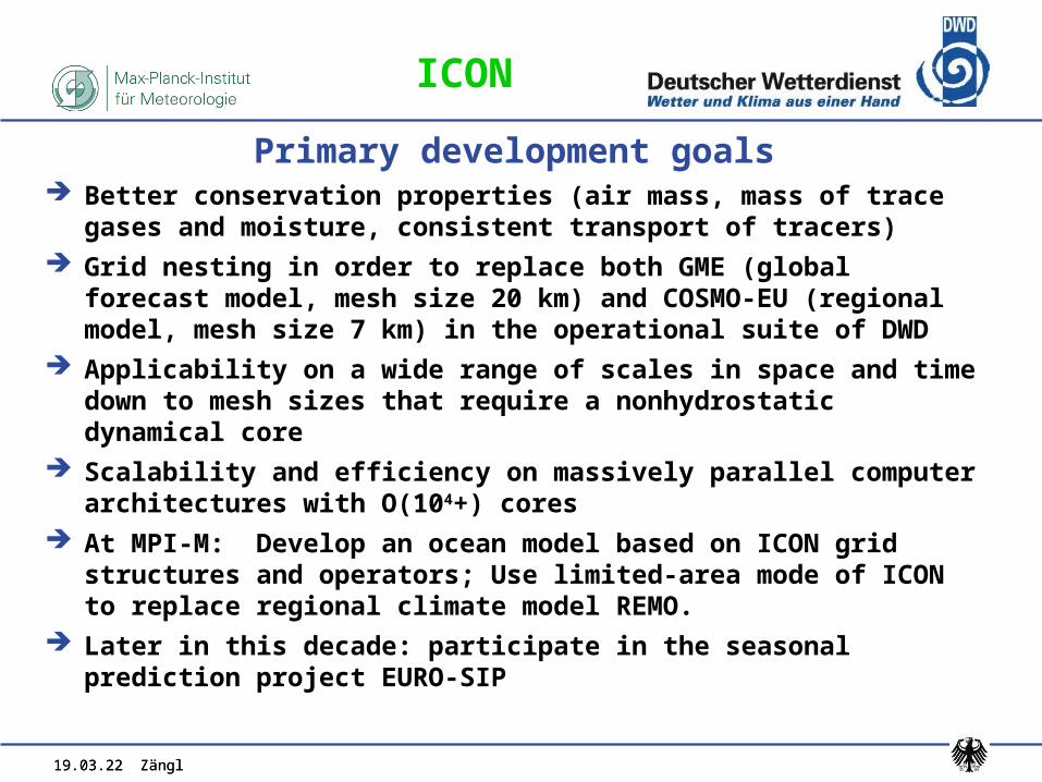
Primary development goals Better conservation properties (air mass, mass of trace gases and

moisture, consistent transport of tracers) Grid nesting in order to replace both GME (global forecast model, mesh

size 20 km) and COSMO-EU (regional model, mesh size 7 km) in the operational suite of DWD

Applicability on a wide range of scales in space and time down to mesh sizes that require a nonhydrostatic dynamical core

Scalability and efficiency on massively parallel computer architectures with O(104+) cores

At MPI-M: Develop an ocean model based on ICON grid structures and operators; Use limited-area mode of ICON to replace regional climate model REMO.

Later in this decade: participate in the seasonal prediction project EURO-SIP

ICON

19.04.23 Zängl19.04.23 Zängl

0)(

0)(

)(

vv

vpdnn

vpdn

tn

vt

vt

gz

cz

wwvwwv

t

wn

cz

vw

n

Kvf

t

v

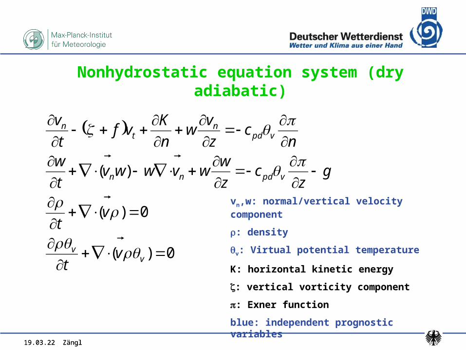
vn,w: normal/vertical velocity component

: density

v: Virtual potential temperature

K: horizontal kinetic energy

: vertical vorticity component

: Exner function

blue: independent prognostic variables

Nonhydrostatic equation system (dry adiabatic)

19.04.23 Zängl

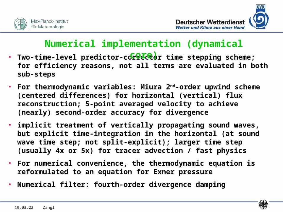
• Two-time-level predictor-corrector time stepping scheme; for efficiency reasons, not all terms are evaluated in both sub-steps

• For thermodynamic variables: Miura 2nd-order upwind scheme (centered differences) for horizontal (vertical) flux reconstruction; 5-point averaged velocity to achieve (nearly) second-order accuracy for divergence

• implicit treatment of vertically propagating sound waves, but explicit time-integration in the horizontal (at sound wave time step; not split-explicit); larger time step (usually 4x or 5x) for tracer advection / fast physics

• For numerical convenience, the thermodynamic equation is reformulated to an equation for Exner pressure

• Numerical filter: fourth-order divergence damping

Numerical implementation (dynamical core)

19.04.23 Zängl

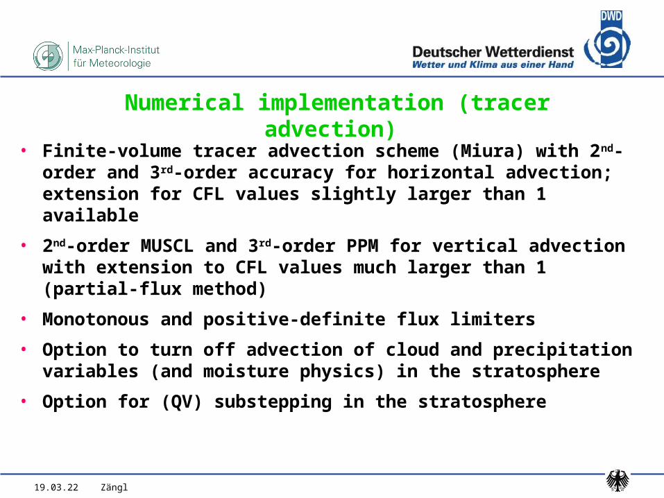
• Finite-volume tracer advection scheme (Miura) with 2nd-order and 3rd-order accuracy for horizontal advection; extension for CFL values slightly larger than 1 available

• 2nd-order MUSCL and 3rd-order PPM for vertical advection with extension to CFL values much larger than 1 (partial-flux method)

• Monotonous and positive-definite flux limiters

• Option to turn off advection of cloud and precipitation variables (and moisture physics) in the stratosphere

• Option for (QV) substepping in the stratosphere

Numerical implementation (tracer advection)

19.04.23 Zängl

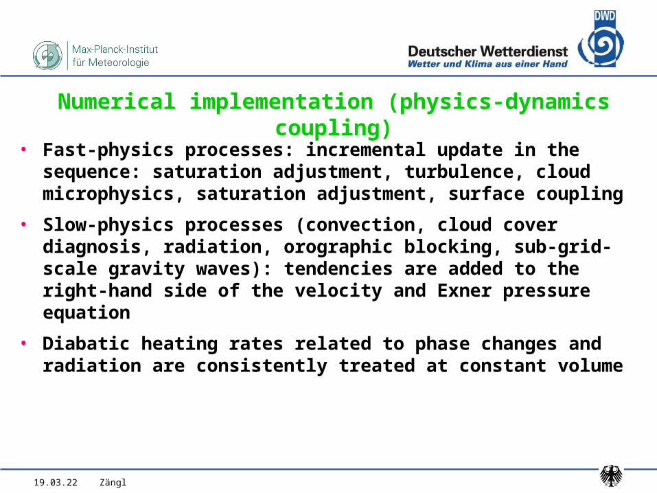
• Fast-physics processes: incremental update in the sequence: saturation adjustment, turbulence, cloud microphysics, saturation adjustment, surface coupling

• Slow-physics processes (convection, cloud cover diagnosis, radiation, orographic blocking, sub-grid-scale gravity waves): tendencies are added to the right-hand side of the velocity and Exner pressure equation

• Diabatic heating rates related to phase changes and radiation are consistently treated at constant volume

Numerical implementation (physics-dynamics coupling)

• Precompute for each edge (velocity) point at level the grid layers into which the edge point would fall in the two adjacent cells

Special discretization of horizontal pressure gradient (apart from conventional method; Zängl 2012, MWR)

dashed lines: main levelspink: edge (velocity) pointsblue: cell (mass) points

A

S

19.04.23 Zängl

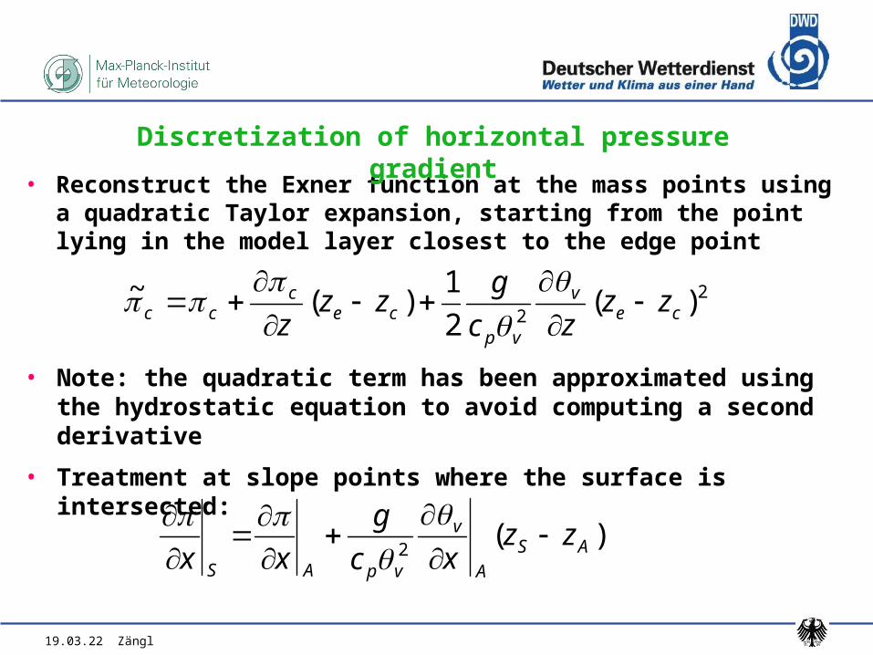
• Reconstruct the Exner function at the mass points using a quadratic Taylor expansion, starting from the point lying in the model layer closest to the edge point

Discretization of horizontal pressure gradient

22

)(2

1)(~

cev

vpce

ccc zz

zc

gzz

z

• Note: the quadratic term has been approximated using the hydrostatic equation to avoid computing a second derivative

• Treatment at slope points where the surface is intersected:

)(2 AS

A

v

vpAS

zzxc

g

xx

19.04.23 Zängl

19.04.23 Zängl

• Highly idealized tests with an isolated steep mountain, mesh size 300 m: atmosphere-at-rest and generation of nonhydrostatic gravity waves

• Jablonowski-Williamson baroclinic wave test with/without grid nesting

• DCMIP tropical cyclone test with/without grid nesting

• Real-case tests with interpolated IFS analysis data

Selected experiments and results

19.04.23 Zängl

atmosphere-at-rest test, isothermal atmosphere, results at t = 6h

vertical wind speed (m/s), potential temperature (contour interval 4 K)

circular Gaussian mountain, e-folding width 2 km, height: 3.0 km (left), 7.0 km (right)

maximum slope: 1.27 (52°) / 2.97 (71°)

19.04.23 Zängl

19.04.23 Zängl

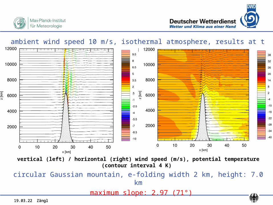
ambient wind speed 10 m/s, isothermal atmosphere, results at t = 6h

vertical (left) / horizontal (right) wind speed (m/s), potential temperature (contour interval 4 K)

circular Gaussian mountain, e-folding width 2 km, height: 7.0 km

maximum slope: 2.97 (71°)

19.04.23 Zängl

19.04.23 Zängl

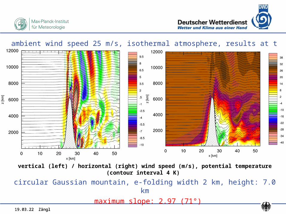
ambient wind speed 25 m/s, isothermal atmosphere, results at t = 6h

vertical (left) / horizontal (right) wind speed (m/s), potential temperature (contour interval 4 K)

circular Gaussian mountain, e-folding width 2 km, height: 7.0 km

maximum slope: 2.97 (71°)

19.04.23 Zängl

19.04.23 Zängl

ambient wind speed 7.5 m/s, multi-layer atmosphere, results at t = 6h

vertical (left) / horizontal (right) wind speed (m/s), potential temperature (contour interval 2 K)

3D Schär mountain, height: 4.0 km, peak-to-peak distance 4.0 km

maximum slope: 2.73 (70°)

19.04.23 Zängl

19.04.23 Zängl

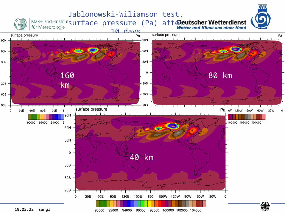
Jablonowski-Wiliamson test, surface pressure (Pa) after 10 days

19.04.23 Zängl

160 km 80 km

40 km

19.04.23 Zängl

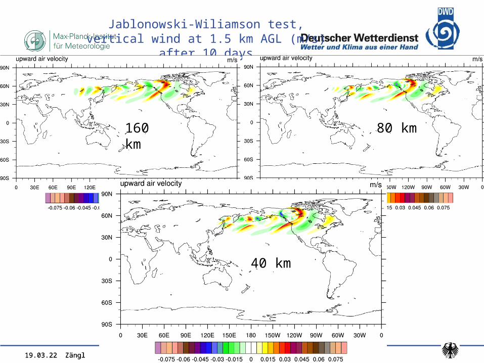
Jablonowski-Wiliamson test, vertical wind at 1.5 km AGL (m/s) after 10 days

19.04.23 Zängl

160 km 80 km

40 km

19.04.23 Zängl

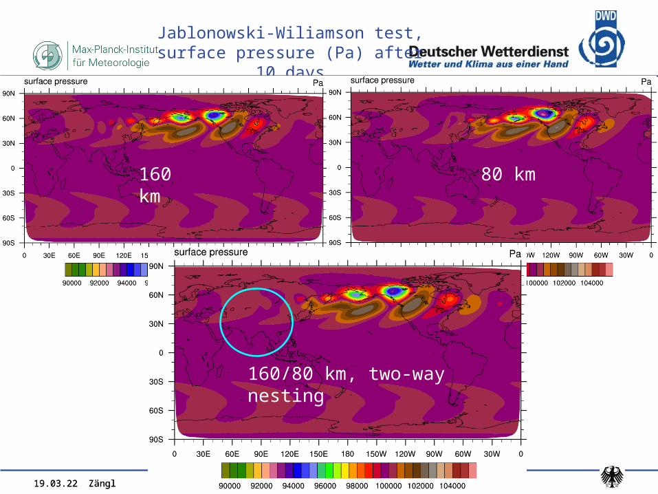
Jablonowski-Wiliamson test, surface pressure (Pa) after 10 days

19.04.23 Zängl

160 km 80 km

160/80 km, two-way nesting

19.04.23 Zängl

DCMIP tropical cyclone test with NWP physics schemes, evolution over 12 days

Absolute horizontal wind speed (m/s)

Left: single domain, 56 km; right: two-way nesting, 56 km / 28 km

19.04.23 Zängl

19.04.23 Zängl

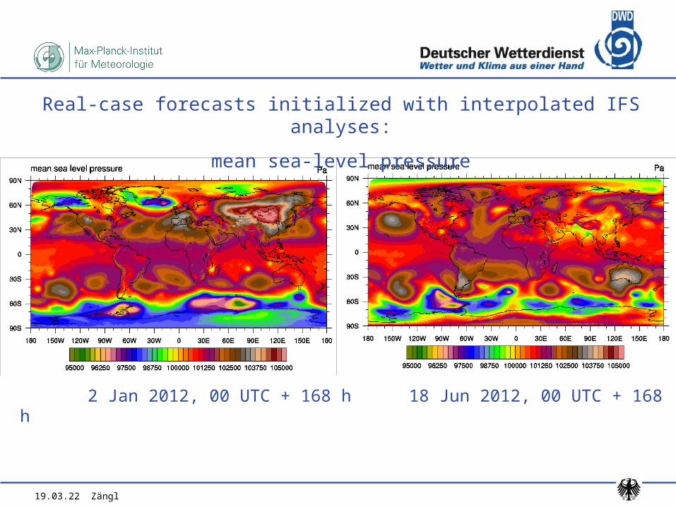
Real-case forecasts initialized with interpolated IFS analyses:

mean sea-level pressure

2 Jan 2012, 00 UTC + 168 h 18 Jun 2012, 00 UTC + 168 h

19.04.23 Zängl

Real-case forecasts initialized with interpolated IFS analyses:

temperature at 10 m AGL

2 Jan 2012, 00 UTC + 168 h 18 Jun 2012, 00 UTC + 168 h

19.04.23 Zängl

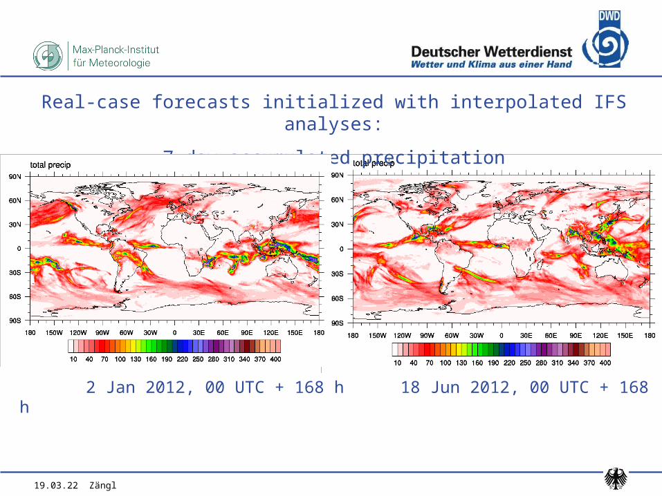
Real-case forecasts initialized with interpolated IFS analyses:

7-day accumulated precipitation

2 Jan 2012, 00 UTC + 168 h 18 Jun 2012, 00 UTC + 168 h

19.04.23 Zängl

WMO standard verification against IFS analysis: 500 hPa geopotential, NHblue: GME 40 km with IFS analysis, red: ICON 40 km with IFS analysis

19.04.23 Zängl

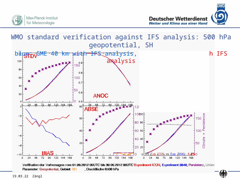
WMO standard verification against IFS analysis: 500 hPa geopotential, SHblue: GME 40 km with IFS analysis, red: ICON 40 km with IFS analysis

19.04.23 Zängl

Summary and conclusions

• The dynamical core of ICON combines efficiency, high numerical stability and improved conservation properties

• The two-way nesting induces very weak disturbances, supports vertical nesting and a limited-area mode

• Forecast quality with full physics coupling is comparable with the operational GME even though systematic testing and tuning is only in its initial phase

• Next major step: coupling with data assimilation

Visit also the ICON posters by Reinert et al. and Ripodas et al.