1989 report no. stan-cs-89-1265 dt i i l i: thesis co 1989 report no. stan-cs-89-1265 dt i i l i:...
TRANSCRIPT

June 1989 Report No. STAN-CS-89-1265
Thesis
DT i i L i: Cow
PARALLEL EXECUTION OF LISP PROGRAMS
NCD by
Joseph Simon Weening
II
Department of Computer Science
Stanford University
Stanford, California 94305
DTIC0 ELECTEfl
* MAR 12 1990
I90 03 12 O"; p.IEu Y
J __ , . ... . . _ u i.

UnclassifiedSECURITY CLASSF;CAT ON O; THIS PAGE
Form ApprovedREPORT DOCUMENTATION PAGE OMB No 0704.0188
la REPORT SECjRIT CASS F'CATION Ic RESTRICTiVE MARK*NGS
2a SECURIr CLASS r-,CA- ON A ,7 OI
-Y 3 DISTRIBuTiON AVALABLT v
0; REoOP
2t DECLASS 1 CA -_ON DOAG;AO G SC- E Unlimited Distribution
4 PERFORMING ORGANZAT'ON REPORT NUMBERIS) S MONITORING ORGANIZATON RErOR7 %_%rBEPS,
STAN-CS-89-1265
6a NAME OF PERFORMING ORGANIZATION 6b OFFICE SYMBOL 7a NAME OF MONITORING ORGANiZATON(If applicable)
Computer Science Dept.
6c. ADDRESS (City, State, -" ZIP Code) 7b ADDRESS (City, State, and ZIP Code)
Stanford University
Stanford, CA 94305
8a NAME OF FUNDING; SPONSORING 8b OFFICE SYMBOL 9 PROCUREMENT INSTRUMENT IDENTIFICATION NUMBER
ORGANIZATION (If applicable)
DARPA N00039-84-C-0211
8c. AODRES (City, State, and ZIP Code) 10 SOURCE OF FUNDING NUMBERS
PROGRAM PROJECT TASK i WORK UNIT
Arlington, VA ELEMENT NO NO NO ACCESSION NO
11 TITLE (Include Security Classification)
Parallel Execution of Lisp Programs
12 PERiONAL AUTHOR(S)Joseph Simon Weening
13a TYPE OF REPORT 73b 'TIME COVERED 14 DATE OF REPORT (Year, Month, Day) 115 PAGE COUNT
Thesis FROM TO 1989, June 92
16 SUPPLEMENTARY NOTATION
17 COSATI CODES 18 SUBJECT TERMS (Cont iue on reverse if necessary and identify by block number)
FIELD GROUP SUB-GROUP
19 ABSTRACT (Continue on reverse if necessary and identify by block number)
Please see other side for abstract...
20 DSRPIBLU ON A-A AB. -Y O ABS-ACT ABSTRACT SEC AR'' CASS'-CA" ON
C] JNCASSIF ED A,,. V1i7ED -- SAME AS RP' C Z YC .SEQS'2a NAME OT RESPOJSB.E NDv',DuA. 22b "ELEPHONE (Include Area Cope) 22c OFFCE SY'0BO.
John McCarthy 723-2273 (!5)
DD Form 1473, JUN 86 Previous editions are obsolete SECpP - C.aSS CA O© -- "
S/N 0102-LF-014-6603
Unclassified
This dissertation considers several issues in the execution of Lisp programs on shared-memory multiprocessors. An overview of constructs for explicit parallelism in Lisp isfirst presented. The problems of partitioning a program into processes and schedulingthese processes are then described, and a number of methods for performing theseare proposed. These inc!uie cutting off process creation based on properties of thecomputation tree of the program, and basing partitioning decisions on the state ofthe system at runtime instead of the program.
An experimental study of these methods has been performed using a simulatorfor parallel Lisp. The simulator, written in Common Lisp using a continuation-passing style, is described in detail. This is followed by a description of the exper-iments that were performed and an analysis of the results. Two programs are usedas illustrations-a Fast Fourier Transform, which has an abundance of parallelism,and the Cocke-Younger-Kasari parsing algorithm, for which good speedup is not aseasy to obtain. The difficulty of using cutoff-based partitioning methods, and thedifferences between vaxious scheduling methods, are shown.
A combination of partitioning and scheduling methods which we call dynamicpartitioning is analyzed in more detail. This method is based on examining themachine's runtime state; it requires that the programmer only identify parallelism inthe program, without deciding which potential parallelism is actually useful. Severaltheorems are proved providing upper bounds on the amount of overhead producedby this method. -We conclude that for programs whose computation trees have smallheight relative to their total size, dynamic partitioning can achieve asymptoticallyminimal overhead in the cost of process creation.
0O Form 1473, JUN 86 Re.ersel SECURITY CLASSIFICATICNI OF THIS DAGE
PARALLEL EXECUTION OF LISP PROGRAMS
A DISSERTATION
SUBMITTED TO THE DEPARTMENT OF COMPUTER SCIENCE
AND THE COMMITTEE ON GRADUATE STUDIES
OF STANFORD UNIVERSITY
IN PARTIAL FULFILLMENT OF THE REQUIREMENTS
FOR THE DEGREE OF
DOCTOR OF PHILOSOPHY
ByJoseph Simon Weening
June 1989

( Copyright 1989 by Joseph Simon Weening
All Rights Reserved
ii

I certify that I have read this dissertation and that in my
opinion it is fully adequate, in scope and in quality, as a
dissertation for the degree of Doctor of Philosophy.
,7 1 John McCarthy(Principal Adviser)
I certify that I have read this dissertation and that in my
opinion it is fully adequate, in scope and in quality, as a
dissertation for the degree of Doctor of Philosophy.N!
VR'-6ard P. (labrig
I certify that I have read this dissertation and that in my
opinion it is fully adequate, in scope and in quality, as a
dissertation for the degree of Doctor of Philosophy.
J rffey D. Ullman
Approved for the University Committee on Graduate
Studies:
Dean of Graduate Studies
iii

Abstract
This dissertation considers several issues in the execution of Lisp programs on shared-memory multiprocessors. An overview of constructs for explicit parallelism in Lisp isfirst presented. The problems of partitioning a program into processes and schedulingthese processes are then described, and a number of methods for performing theseare proposed. These include cutting off process creation based on properties of thecomputation tree of the program, and basing partitioning decisions on the state ofthe system at runtime instead of the program.
An experimental study of these methods has been performed using a simulatorfor parallel Lisp. The simulator, written in Common Lisp using a continuation-passing style, is described in detail. This is followed by a description of the exper-iments that were performed and an analysis of the results. Two programs are usedas illustrations-a Fast Fourier Transform, which has an abundance of parallelism,and the Cocke-Younger-Kasami parsing algorithm, for which good speedup is not aseasy to obtain. The difficulty of using cutoff-based partitioning methods, and thedifferences between various scheduling methods, are shown.
A combination of partitioning and scheduling methods which we call dynamicpartitioning is analyzed in more detail. This method is based on examining themachine's runtime state; it requires that the programmer only identify parallelism inthe program, without deciding which potential parallelism is actually useful. Severaltheorems are proved providing upper bounds on the amount of overhead producedby this method. We conclude that for programs whose computation trees have smallheight relative to their total size, dynamic partitioning can achieve asymptoticallyminimal overhead in the cost of process creation.
iv

Acknowledgements
First I would like to thank my advisor, Professor John McCarthy, and the othermembers of my reading committee, Professors Richard Gabriel and Jeffrey Ullman,for their support throughout the years of researching and writing this dissertation,and their criticisms and comments on the text. Dick Gabriel, especially, providedmany hours of his time listening to early versions of my ideas.
Much of the work described in Chapter 5 was done jointly with Dan Pehoushek,and the discovery of the ideas presented there would not have occurred without hisdedicated persistence in fine-tuning the Qlisp system.
Other members of John McCarthy's formal reasoning and Qlisp research groupsprovided much encouragement and friendship, particularly Igor Rivin, Carolyn Tal-cott and Ramin Zabih.
Professor Robert Halstead of MIT provided me with a complete copy of his Multi-lisp system, the study of which was quite useful. Professor Anoop Gupta of Stanfordsuggested a number of improvements to the text of the dissertation.
Financial support for my graduate study at Stanford came from the National Sci-ence Foundation, the Fannie and John Hertz Foundation, and the Defense AdvancedResearch Projects Agency.
Acoession ForNTIS GRA&I
DTIC TAB QUnannounced 0Jastiftostio-
ByDistribution/
AvaT1abiUty CodesXAvai a nd/or
Diet Specialv I

Contents
Abstract iv
Acknowledgements V
1 Parallel Lisp 11.1 Shared memory................................... 21.2 Parallel argument evaluation..................... ........ 31.3 Multilisp............ .............................. 4
1..3.1 Futures .. .. .. ... .... ... ... ... ... .... ... 41.3.2 Delayed evaluation. .. .. .. ... .... ... ... ... ... 61.3.3 Synchronization. .. .. .. .. .... ... ... ... ... ... 71.3.4 Multischemne,.. .. .. .. ... ... ... ... ... .... ... 7
1.4 Qlisp .. .. .. .. ... ... .... ... ... ... ... .... ...1.4.1 Process closures. .. .. .. .. .... ... ... ... ... ... 91.4.2 Speculative computation .. .. .. .. ... .... ... ..... 10
1.5 Other versions of Parallel Lisp. .. .. .... ... ... ... ..... 101.5.1 PaiLisp. .. .. ... ... ... ... .... ... ... ..... 101.5.2 ZLISP .. .. .. ... ... ... ... ... .... ... ..... 11
1.6 Conclusions on language design .. .. .. ... ... ... ... ..... 11
2 Partitioning and scheduling methods 132.1 Computation graphs .. .. .. ... ... ... .... ... ... .... 142.2 Notation for describing performance .. .. .. .. ... ... ... ... 162.3 Partitioning methods .. .. .. .. ... .... ... ... ... ..... 17
2.3.1 Height cutoff .. .. .. ... ... ... .... ... ... .... 172.3.2 Depth cutoff. .. .. .. .. ... ... .... ... ... ..... 19
2.4 Scheduling methods. .. .. .. .. ... .... ... ... ... ..... 212.5 Dynamic partitioning. .. .. .. .. .... ... ... ... ... ... 22
vi

3 A Parallel Lisp Simulator 253.1 A continuation passing Lisp interpreter ..................... 263.2 An interpreter for Common Lisp .......................... 30
3.2.1 Environments ....... ........................... 303.2.2 The global environment ...... ..................... 313.2.3 Function application ...... ....................... 313.2.4 Special forms ....... ........................... 333.2.5 Multiple values ....... .......................... 353.2.6 Timing statistics ....... ......................... 35
3.3 Parallel Lisp constructs ................................ 363.3.1 Scope and extent issues ............................ 37
3.4 Simulating the parallel machine ...... ..................... 393.4.1 Processors ....... ............................. 403.4.2 The scheduler ....... ........................... 413.4.3 Processes ........ ............................. 423.4.4 Process closures ....... .......................... 43
3.5 Miscellaneous details ....... ........................... 433.5.1 Jse of symbols ....... .......................... 433.5.2 Preprocessing of definitions ..... ................... 443.5.3 Interpreted primitives ...... ...................... 453.5.4 Top level .................................. ... 463.5.5 Memory allocation and garbage collection .............. 46
3.6 Accuracy and performance ...... ........................ 463.6.1 Accuracy of simulated times ........................ 473.6.2 Speed of the simulator ...... ...................... 48
3.7 A Parallel example ....... ............................ 50
4 Experimental results and analysis 574.1 The Fast Fourier Transform ...... ....................... 574.2 The CYK parsing algorithm ...... ....................... 65
5 Analysis of dynamic partitioning 735.1 Process creation behavior ....... ........................ 735.2 Extending the basic result ....... ........................ 785.3 Making use of dynamic partitioning ........................ 80
6 Conclusions 81
Bibliography 83
vii

Chapter 1
Parallel Lisp
Multiprocessor systems have introduced a new set of challenges in the implementationof programming languages. Attempts to make use of parallelism have resulted in avariety of programming models. One way in which these approaches differ is whetherthey support implicit or explicit parallelism in programs.
Implicit parallelism insulates the programmer from the details of the parallel en-vironment. The language support system, at compile time or runtime, decides howto translate the constructs of the programming language into concurrent operationson the parallel machine. This approach has been applied both to existing languages,and to new languages designed to take better advantage of a parallel environment.
Explicit parallelism lets the programmer specify what computations are to beperformed in parallel. With language constructs for specifying concurrency, a pro-grammer can make use of knowledge about parallelism in a program that an automaticsystem might not be able to deduce. Existing pogramming languages have been ex-tended with constructs that specify parallel behavior, and new languages have beenproposed that include explicit parallelism.
This dissertation is about explicit parallelism applied to Lisp. Lisp is a languagefor symbolic data processing that has been used primarily in artificial intelligence [20].Many problems for which Lisp is used require large amou:its of computation, soexecuting Lisp efficiently on parallel computers is an important problem.
The remainder of this introductory chapter describes our model of computation,and presents several sets of language constructs that have been proposed in parallelLisp systems. Chapter 2 introduces the concepts of partitioning and scheduling,which are the main focus of our research. Chapter 3 describes a simulator for parallelLisp which was designed to test strategies for program execution, and discusses themerits and drawbacks of using simulation as an experimental tool. Experimentsusing the simulator are presented in Chapter 4. The main observation made from
CHAPTER 1. PARALLEL LISP
these experiments is the success of a strategy Otat we call "dynainic partitioning."and an analysis of this method is done in Chapter .5. Finally. Chapter 6 summarizesthe work that has been done and points out areas that require further investigation.
1.1 Shared memory
This rcsearch coi 1,iders multiprocessors with shared memory, in which the access timefor all memory words is uniform. In other words, there should be no penalty whena program uses "global" memory as opposed to "local" memory. This assumptionfrees the programmer from the burden of reorganizing data structures in order toimprove the speed of memory access, and is therefore less of a departure from theprogramming model used for Lisp on sequential processors than distributed memorymodels. Our use of the term "shared memory" will always include this assumptionof uniform access time.
While shared memory with uniform access time is useful as a programming model,it may not be possible to build multiprocessors having this characteristic with morethan a limitec, number of processors, using current techniques in hardware design.(The limit seems to be in the range of tens to hundreds of processors.) To studyparallel machines with a large number of processors therefore, we may have to allowa non-uniform memory model. On the other hand, several shared-memory machineswith a small number of processors have been built and are now commercially avail-able. The methods for programming these machines are still in an early stage ofdevelopment, and this area is where we hope to make a contribution.
The usual methods of Lisp implementation lead us to prefer a shared-memoryapproach. Lisp is a call-by-value language, but the values that are passed are oftenpointers to data structures of arbitrary s.ze. One of the things that has made Lisp sucha success is that the management of these data structures (allocation and reclamationby garbage collection) is completely automatic. We do not want to remove thisstrength of the -anguage by introducing programming tasks that are extraneous to theactual problems being solved, such as the explicit distribution of data and processesto particular parts of memory in order to improve performance. Automating thesetasks is a possibility for future research.
Garbage collection is an integral part of Lisp systems, but we do not discuss it inthis dissertation. Implementing garbage collection on a multiprocessor is a challengingprobiem and the subject of much ongoing research.

1.2. PARALLEL ARG UMENT EVX'L UATION 3
1.2 Parallel argument evaluation
The most obvious place in which to introduce parallelism in Lisp programs is inthe evaluation of arguments to functions. Especially in code written in a '"functional"style, most computation in Lisp programs consists of functions calling other functionsin order to perform subcomputations, and often no specific execution order is requiredfor correct exer f ion. For example, in an arithmetic expression such as
(+ (log x) (log y)),
the calls to (log x) and (log y) may be performed in either order, or in parallel.The main problem with parallel argument evaluation arises when we allow side
effects in programs. In some versions of Lisp, the order of evaluation of functionarguments is defined by the language (e.g., in Common Lisp [24] it is left-to-right), soside effects in the first function call must happen before those in the second. In otherversions of Lisp (e.g., Scheme [1]), the order is unspecified, but it is still assumedthat the arguments are evaluated one at a time. For instance, if two argumentsto a function are calls to cons, then the usual sequential implementation, in whichcons performs side effects to a list of free cells, is not correct for parallel execution.There will be a critical region in the code for cons between the time when the oldfree-list pointer is read from memory and the time when the new free-list pointeris stored. If several processors execute the code in this region simultaneously, theywill all end up allocating the same cell. Correct behavior of cons can be ensured inin several ways: adding synchronization code around the critical region to preventsimultaneous execution; using special atomic hardware instructions that remove theneed for a critical region; or having cons allocate from a separate free list for eachprocessor, which also eliminates the critical region.
It is not too hard to avoid the problem of side effects when implementing the pre-defined Lisp functions such as cons, so that they may always be called concurrently,but synchronization problems may remain in user-written functions that perform sideeffects. Therefore, parallel argument evaluation is dangerous when the forms evalu-ated in parallel may be calls to arbitrary functions. Some Lisp systems avoid thisdanger by restricting the language to be side-effect free. We feel that side effectsand parallelism can coexist, by not making parallel argument evaluation the defaultbehavior of the system, but providing language constructs by which a programmercan explicitly state that concurrency is allowable.
Another important reason for requiring parallel argument evaluation to be explicitis the cost associated with starting a computation on another processor. On mostmultiprocessors, it is several times the cost of a function call, and adding this cost

4 CHAPTER 1. P.ARALLEL LISP
to each function call would multiply the total runping time by a significant constantfactor. We will examine several techniques that avoid much of this potential overheadcost.
1.3 Multilisp
Multilisp [13] is a system begun in 1980 by Halstead at the Massachusetts Instituteof Technology. Most of its sequential Lisp constructs come from Scheme [1] [26],although some features of Scheme such as continuations are not supported. Alongwith language constructs that add parallelism to the basic Lisp, Halstead and his col-leagues have designed and implemented a prototype shared-memory multiprocessor,Concert [4], on which Multilisp runs.
One of Multilisp's forms for specifying parallel execution is pcall, which imple-ments parallel argument evaluation as described in the previous section. The form
(pcall fun arg, . . . arg)
causes the expressions fun and argl,..., argn to be evaluated in separate processes;'once these processes finish, the value of fun is applied to the values of argl,..., argn.(Although fun is usually just a symbol that names a function, Scheme allows anarbitrary expression in this position, and Multilisp evaluates it in parallel with thefunction arguments.) Using pcall, our example from the previous section would bewritten as
(pcall + (log x) (log y)).
1.3.1 Futures
Multilisp's other form for creating parallel processes is future. When (future expr)is evaluated in a program, a new process is created to evaluate expr. Unlike pcall,which waits for the processes that it creates to finish and then uses the values thatthey return, future allows the original process to continue execution. In place ofthe value that expr will produce, future returns an object called a future, whichrepresents that value. In the tagged-pointer data representation used by Multilisp, afuture is a pointer with a special tag indicating that it is not an ordinary data object,and pointing to the process that is computing the actual object's value. We will callthis the future's "associated process."
For most purposes, a future is not distinguishable from the data object that willbe returned by its associated process, because Multilisp ensures that whenever an
'Multilisp calls these "tasks", but we use the term "processes" throughout this dissertation.
1.3. MULTILISP 5
operation needs the value of the object represented by a future, if the associatedprocess has not yet finished, then the process requiring the value is suspended until
that value is available. For example, the expression
(+ (future (log x)) (log y))
will start a new process to evaluate (log x) and continue in the original process toevaluate (log y). Some concurrency is therefore achieved by performing these callsin parallel. After the call to (log y) returns, however, the '+' function is called; itsarguments are the future that was created for (log x) and the value of (log y). The'+' function cannot add a future to a number; it requires the actual value associatedwith the future. It therefore performs an operation that Multilisp calls "touching" onboth of its arguments, to ensure that they are normal Lisp objects, not futures. If anobject that is touched is a future, then if its associated process is finished, the valuethat the process returned is used; if the associated process is still executing, then thetouching process is suspended, and is awakened when the value has been computed.In either case, the touching operation eventually returns the value associated withthe future.
Aside from the suspension and resumption of the process, there is no semanticdifference between what happens when future is used and what would have happenedhad the original expression been (+ (log x) (log y)). As in parallel argumentevaluation, the presence of side effects may require a specific execution order andtherefore make the use of future inappropriate. Several of Halstead's students havestudied methods for automatically and safely inserting future into programs, inboth the side-effect free case [12] (where adding future is always safe, but should beavoided when it does not yield any parallelism), and in some programs that perform
side effects [30].
One important benefit of futures is the way in which they are treated by formsthat do not require the values of their arguments. These are forms which will performthe same operations no matter what arguments they are given. A good example iscons, which allocates a cons cell and stores its two arguments into the cell, withoutexamining the arguments. If a future is passed as an argument to cons, Multilispdoes not wait for the object represented by the future to be computed; instead, itstores the future into the cons cell just like any other object. The future's associatedprocess may therefore execute in parallel with other processes that pass around thisvalue, as long as they do not perform operations that "touch" the value as described
above.
Lisp operations that manipulate values without touching them include cons andother functions that construct data structures, assignment operations such as setq,

6 CHAPTER 1. PARALLEL LISP
and the operations of passing argument values to functions and returning their results.That is to say, a future can be returned from a function and passed to another, allwithout waiting for the object that it represents to be determined.
1.3.2 Delayed evaluation
The concept of futures is related to that of "delayed" or "lazy" evaluation, which wasfirst proposed for Lisp by Henderson and Morris [15], and is discussed as an aspectof parallel programming by Friedman and Wise [6]. In delayed evaluation, functionslike cons, that do not require the values of their arguments, do not evaluate theirarguments at all. In place of each argument value, they use an object that representsthe computation of that value. These objects are recognized by functions that dorequire an actual value, and at that point, computation of the value is performed.Lazy evaluation can be used to define "infinite data structures." For example, thefollowing program represents the infinite set of natural numbers by a list, which isonly computed as far as any part of the program examines it:
(defun natnum (n)(cons n (natnum (+ n 1))))
(setq natural-numbers (natnum 0))
In Multilisp, cons does evaluate its arguments, but delayed evaluation can be in-dicated by a delay expression. The above definition would be written in Multilispas:
(defun natnum (n)(cons n (delay (natnum (+ n 1)))))
(setq natural-numbers (natnum 0))
The same tagged pointer that is used to represent a future can be used to implementdelayed evaluation. The difference between lazy evaluation and the use of futures,also known as "eager" evaluation, is that the lazy method waits to compute a valueuntil it is required, while the eager method computes it in parallel with the rest ofthe program, on the assumption that the value will be needed. This assumption maybe false; the object might be stored in a data structure and never examined, or maybe passed as an argument to a function but ignored. Eager evaluation can not alwaysbe substituted for delayed evaluation; in the example of the infinite data structureabove, substituting future for delay might cause an infinite sequence of processesto be created. (The method used for scheduling processes would determine whetherthis would actually occur.)
1.4. QLISP 7
1.3.3 Synchronization
Futures provide implicit synchronization of processes because the consumer of a datavalue is forced to wait until the value has been produced. Such synchronization isdone by Multilisp and need not be specified by the programmer, so the code forparallel programs is often very clean and consise-it may be the same as the code fora sequential version of the program, except for future added wherever concurrencyis desired. However, sometimes a programmer wishes to use side effects or destructiveoperations on data structures, and in these situations the synchronization providedby futures is not enough.
To allow this style of programming, Multilisp provides locks. These are objectson which processes may perform wait and signal operations. If a process waits ona lock that is busy, it is suspended using the same mechanism that causes processesto wait for futures, and it is resumed when a signal causes the lock to be made free.
Multilisp also has two atomic memory operations, replace and replace-if-eq,which can be used to perform synchronization.
1.3.4 Multischeme
Miller, a student of Halstead, has implemented a system called Multischeme [21].Miller's work pays particular attention to implementation strategies for various as-pects of the system, and is the basis for a parallel Lisp system that has been imple-mented on the BBN Butterfly.
Multischeme introduces a data type called placeholders that are a generaliza-tion of Multilisp's futures. Placeholders can be used for both the delayed and eagerevaluation methods described above, and they are "invisible" in the sense that a ref-erence to a placeholder automatically returns the associated data object, or suspendsthe process making the reference until the placeholder is determined. In addition,placeholders can be mutable, meaning that the object they refer to may be changedeven after its initial value is determined. If t',ere are several references to such aplaceholder, all of them will automatically refer to the new object.
Using placeholders, Multischeme can implement logic variables (as in Prolog), aswell as a variety of other programming constructs.
1.4 Qlisp
In 1984, Gabriel and McCarthy proposed the Qlisp language [8]. The name arisesfrom the queue of processes kept in shared memory, to hold work that is available for
S CHAPTER 1. PARALLEL LISP
idle processors. As modified in later documents [9]. Qlisp is an extension of CommonLisp wvith several forms for the creation and control of parallel processes.
One of the principal points of the Qlisp philosophy is that process creation canbe made conditional on arbitrary propositions that may be evaluated during theexecution of a program. This is important for several reasons:
" The creation of a process may involve overhead that can be avoided when itdoes not contribute to increased parallelism.
" Creating too many processes results in excessive use of memory, and for somecomputations not enough memory will be available unless process creation iscontrolled at runtime.
Instead of specifying the creation of processes at a point where a function is called,as in the pcall and future forms of Multilisp, Qlisp's primary construct for creatingparallel processes is qlet, a parallel form of the let form. The expression
(qlet prop((var 1 form1 )
(var, form,.))body)
first causes the evaluation of the proposition prop to occur, and then either evaluatesthe forms form1 , ... , form,, sequentially, if prop's value is nil; or evaluates them in
separate parallel processes, if it is non-nil. Each of these processes returns the valueof the form that it has evaluated, and these values are bound to the correspondingvariables. When all of the processes have finished, the body of the qlet form isevaluated in the context established by these bindings.
Sometimes, additional concurrency may be gained by starting evaluation of theqlet body before all of these processes have returned their values. This is the casewhen, for example, the body performs some initialization before using any of thevalues, or if a value is used by a function like cons that does not need to "touch"it, as discussed above. Evaluation of the body in parallel with the new processescreated by qlet is specified by having prop evaluate to the symbol :eager. In thiscase, Qlisp creates a future, with the same properties as Multilisp's futures, for eachof the bound variables, and associates it with the process computing that variable'svalue. Evaluation of the body then occurs with the variables bound to these futures.
Note that it is possible for a process associated with a future to continue executingafter the qlet form that created it has finished. Therefore, Qlisp must accept the

1.4. QLISP 9
possibility of accesses to futures occuring anywhere in a program. not just inside thebodies of qlet forms.
Although the syntax is different, Qlisp's qlet is semantically equivalent to Multi-lisp's pcall and future constructs. Each can be written in terms of the others by asimple source transformation.
1.4.1 Process closures
Qlisp introduces several new concepts that are not found in other versions of parallelLisp. One of these is the process closure, defined by the qlambda special form. Itprovides three important features:
1. Encapsulation of a lexical environment. This is done in the same way as ordinaryclosures provided by Common Lisp's lambda.
2. Mutual exclusion. A process closure, which can be called as a function, ensuresthat its body is not executing in more than one process at a time. Qlisp saves thearguments of calls to process closures that occur while a previous call is still inprogress, and evaluates the calls sequentially. The code inside a process closuremay therefore perform side effects without the problems of non-determinacy.
3. Parallel execution. When a process closure is called as a function, it immediatelyreturns a future. The caller may then proceed with other work, using the futureto represent the value that will eventually be returned by the call to the processclosure. If the calling process needs to wait for the process closure to finish, itcan pass the future as an argument to a value-requiring form, and thus suspenduntil the process closure returns a value for the future.
The syntax of qlambda is the same as that of lambda, except that a propositionalparameter is added, as with qlet, to allow a runtime decision about whether to useparallelism. If this proposition evaluates to nil, then property (3) described abovedoes not hold; the process closure still maintains mutual exclusion, but when it iscalled, the calling process executes the body of the qlambda form. If the propositionis non-nil, a new process is created along with the closure for the qlambda, and thebodies of calls to the process closure are executed in this process.
Qlambda is a higher-level synchronization construct than the locks provided byMultilisp. (Qlisp also provides low-level locks, for applications in which their efficiencyis crucial.) The semantics of qlambda is very similar to that of monitors [16], combinedwith the object-oriented features that the encapsulation of a lexical environmentprovides.

10 CHAPTER 1. PARALLEL LISP
1.4.2 Speculative computation
Another feature that Qlisp provides is the ability to perform speculative computation,by starting processes when it is possible but not certain that their results will beneeded, and thus making use of processors that would otherwise have nothing to do.
Speculative computation can be used in a problem that has several strategies forsolution, if it is not known which one will be fastest on a given problem instance. Wemay start separate processes to try each of these strategies and use the result of theone that returns first.
When one of these processes finishes, the results of the other processes are notneeded, and it is desirable to terminate those processes rather than allow them tocontinue using resources. The parallel Lisp implementation must provide a mecha-nism for doing this, and a well-defined way of determining which processes are to beterminated when a given process finishes.
Qlisp accomplishes this by extending the meaning of the catch and throw con-structs of Common Lisp. Some such extension is necessary in any case, because weneed to define what it means when a throw occurs in one process but the correspond-ing catch was performed in a different process. To resolve this problem, Qlisp appliesthe principle that (in Common Lisp) each catch can be returned from only once, ei-ther by a throw or by a normal function return. Therefore, any other processes thatmight cause the same catch to return are terminated.
The exact definition of which processes are terminated turns out to be quitecomplicated, and is explored in [9]. (Along with catch and throw, the semanticsof unwind-protect is defined there.) Especially in the presence of side effects andfutures, deciding what is the "right thing" to do is not always clear. This area oflanguage design is still undergoing research.
1.5 Other versions of Parallel Lisp
Several other projects have researched or are now working on various aspects of par-allel Lisp. These include the following.
1.5.1 PaiLisp
Ito and Matsui, at Tohoku University in Sendai, Japan, have defined a language calledPaiLisp, based on the constructs of Multilisp and Qlisp, and implemented a simulatorfor PaiLisp in Common Lisp [18]. PaiLisp uses Scheme as a base language and addsa "kernel" of four basic forms from which the other parallel Lisp constructs can bedefined. The forms in the kernel are:
1.6. CONCLUSIONS ON LANGUAGE DESIGN 11
1. A spawn form to spawn a new process:
2. A version of Scheme's call-with-current-continuation that works as fol-
lows: When a continuation that was created by process P is called by processQ, process P calls the continuation while Q continues with its normal continu-
ation;
3. An exclusive function closure (like the nil version of Qlisp's qlamnbda form);
4. A suspend function to suspend a process. The suspended process can be re-sumed by calling its continuation.
1.5.2 ZLISP
Dimitrovsky, working with the Ultracomputer Group at New York University, has cre-ated a parallel Lisp system called ZLISP that makes effective use of synchronizationconstructs such as the fetch-and-add instruction of the Ultracomputer. His disserta-
tion [5] describes the implementation of the system as well parallel algorithms and
data structures used in ZLISP programs and in ZLISP itself.
1.6 Conclusions on language design
This chapter has been a summary of the work to date in parallel Lisp systems, focusingon extensions to the Lisp language and how they are used in parallel programs.
We believe that the various systems described provide a reasonable foundation forexperimental work.
Some of the language constructs, such as parallel argument evaluation, futures,and process closures, have gained acceptance and seem appropriate tools for use in
parallel Lisp programs. Others, such as the support of speculative computation, are
still unsettled.
Experience with parallel programming is beginning to show that while these lan-
guage constructs are sufficiently powerful, they do not help much in solving the con-
ceptual problems that programmers face when trying to write parallel Lisp programs.
Much work needs to be done in discovering "high-level primitives" that remove theprogrammer from low-level details of process creation and synchronization, while not
sacrificing too much efficiency, since fast execution is the reason that most program-
mers are interested in parallel programming.

12 CHAPTER 1. PARALLEL LISP
Chapter 2
Partitioning and schedulingmethods
There are several stages in the preparation and execution of a parallel program:
" Algorithm design. The overall design of a program and its data structures willhelp to determine whether it will run well on a parallel computer, and it remainsthe programmer's job to specify this aspect of the computation. A parallel algo-rithm can be translated into a program using the language constructs describedin the previous chapter, or using higher-level constructs based on those.
* Partitioning. Not all of the possible parallelism in a program may contributeto an increase in its performance. Some process creations may in fact reduceperformance, because of the additional overhead. We view the parallel algorithmas specifying potential processes, which are computations that may be run inparallel when there is some benefit to doing so. Partitioning is the problem ofchoosing which potential processes to make into actual processes.
* Scheduling. We must also address the problem of which processes to executeat any given time in the computation. Since all of the processors are assumedto be identical in speed and memory access time, it does not generally matterwhere a given process is run; but the choice of which processes wait while othersrun may have an effect on the overall execution time.
We view algorithm design and the identification of parallelism as activities that takeplace before the program is run. These may be done entirely by the programmeror with the help of tools that partially automate the process, including compileralgorithms that detect parallelism. Our main focus is on what happens after the
13
14 CHAPTER 2. PARTITIONING AND SCHEDULING METHODS
parallelism in the program is specified. (Some research has considered identifyingparallelism at runtime as well, for example the ParaTran system described in [28].)
In our model of parallel execution, both partitioning and scheduling happen atruntime. Others have considered doing one or both of these at compile time [14] [23],and that approach has advantages for programs that have predictable behavior. Butfor the kinds of problems that Lisp is typically used to solve, important parametersabout the input data are often not available until runtime and are necessary for goodpartitioning and scheduling decisions.
Partitioning and scheduling need not be independent. A decision about whetherto create a process may depend on the current state of the system as well as prop-erties of the program and the input data. We will investigate several methods thathave this property, as well as methods that separate partitioning and scheduling intoindependent problems.
Several of the language features described in Chapter 1 make the performanceof partitioning and scheduling methods harder to analyze. We can sometimes makestronger statements about programs that avoid these features, so for this reason wedefine the following categories of parallel Lisp programs.
" Non-speculative programs are those that require each process that is startedto run to completion. The computation is not considered finished until allprocesses are done, even if the top-level process has returned a value, whichmay happen when futures are used.
" Non-eager programs, in addition to the above restriction, do not use futures.Non-eager programs use only the basic fork/join style of parallelism providedby pcall in Multilisp or qiet in Qlisp. Programs with futures are harder toanalyze because not all of the work done by a process needs to be finished whenthat process returns a value, and the point at which synchronization occurs maybe difficult or impossible to discover by static analysis of the program.
2.1 Computation graphs
A graphical representation of a computation will help in describing some events thattake place during its execution, and in analyzing partitioning and scheduling methods.For a given execution of a program, we define a computation graph, a directed graphwhere the nodes are processes or portions of sequential execution within a process,and the edges are precedence relations between them. An edge from node .4 to nodeB indicates that execution of B may begin after execution of node A is complete.

2.1. COMPUTATION GRAPHS 15
Labels on the nodes in F. computation graph are used to identify the processin which they occur (,- process's computation might consist of several nodes in thegraph), and when necessary to show what parts of the program they correspond to.
We construct the graph of a computation as follows. A potential process thatcannot create any subprocesses and that never needs to wait for other processes tofinish is a single node. If process P can create processes P1, P2,... , Pi running inparallel, and then will wait for them to finish (using Multilisp's pcall or Qlisp'snon-eager qiet forms), the corresponding portion of the graph is
Edges in such a diagram implicitly point downward, i.e., the lower node is assumedto depend on the completion of the higher node.
The two nodes labeled P represent different portions of sequential execution withinprocess P. Process P may create subprocesses at several points during its execution,and these result in concatenation of such g-aphs. Therefore, the computation graphsof programs of this type (non-eager programs) are series-parallel graphs in general. If,however, each potential process has at most one point at which it can create a set ofsubprocesses, the computation graph will be symmetric-it wi, ,onsist of an out-treeof process creations (forks) and an in-tree of synchronization points (joins). We willoften show just the tree of process creation in this case, and call this a computationtree and draw it as follows.
When eager programming constructs are used (Multilisp's future and Qlisp'seager qiet forms), the computation graphs may become arbitrary DAGs (directedacyclic graphs). The creator of a process need no longer wait for that process tofinish: on the other hand, by passing the future as a data value it is possible for morethan one node in the graph to require the completion of a given node.
16 CHAPTER 2. PAfRTITIONIG AND SCIHEDULING METHODS
2.2 Notation for describing performance
Here we define some notation that we will use in making statements about programperformmnce. A program is a set of Lisp functions that are used to perform somecomputation. We are generally interested in the behavior of a program over a rangeof input values and a variety of configurations of a multiprocessor. We express theseparameters by variables n, a "size" function of the input, and p, the number ofprocessors.
For given values of n and p, let Tscq be the sequential running time (i.e., the timeon a non-parallel machine), and Tpr be the running time on a parallel machine withp processors. We define the overhead time to be
To,head = P Tp r - T.eq.
The overhead time summarizes all of the extra time that is spent because of paral-lelism.
The speedup resulting from the use of a multiprocessor is defined as
S Teq
and the efficiency isE -- Ts--- --
p Tp "
Perfect speedup on p processors is achieved when S = p, or equivalently E = 1.Based on the parallel execution model outlined in Chapter 1, we can divide over-
head time into the following categories.
" Partitioning contributes to overhead when it is performed at runtime. LetTparition be the total time spent evaluating runtime propositions that decidewhen to create a process.
" Process creation requires a certain amount of additiona' time for each processthat is created, in order to allocatc and initialize data structures. If nproc isthe number of processes created (as a function of n and p) and T, is the timerequired to create a single process, then Tcreate = nproc. T,.
* Scheduling requires some time both when a process is created and when aprocessor becomes idle. Some of this is a fixed cost that we can associate withthe creation of a process; we include this in T,. There is also some variationin scheduling time because of contention for data structures that are sharedbetween the processors. Let Tcheduf, represent this portion of the overhead.
2.3. PARTITIONING METHODS 17
" Futures introduce a source of overhead. When the value of a future is required
but is not available, a process is suspended and later resumed. The extra work
required to perform these operations will be called Tfutr.
" Idle time is the amount of time spent waiting for a process to become availble
when there are none ready to run. Tidte is the sum of all of the processors' idle
times.
There are no other sources of overhead time because of the simplifying assumptions
that we made in our parallel execution model. Therefore we can write the equation
Toverhead = Tpartition + Tcreate + Tchedu e + T uture + Tidle.
For non-eager programs, Tuture is always zero, but we expect the other forms ofoverhead to have positive values whenever a program is run on a parallel machine.
We make the distinction between running a program sequentially, which involves
no overhead, and running it in parallel on a one-processor machine, which might
involve all of the above sources of overhead except idle time. In our experiments, the
sequential programs are versions of the parallel programs with all runtime partitioning
tests and creation of processes removed.
We could go one step further, and insist that a program expressing a given parallel
algorithm be compared with the best sequential algorithm for the same problem, even
if the sequential algorithm cannot be sped up as much as the parallel algorithm. This
would provide a better measure of the true performance gain that parallel execution
provides. However, we will not make this comparison because it is not relevant to
our main goal, which is to provide the best possible performance for a given parallel
program. For this, the appropriate base measure is the sequential version of the same
program.
2.3 Partitioning methods
This section describes several partitioning methods that have been proposed for par-
allel Lisp. We will examine the performance of these methods in Chapter 4.
2.3.1 Height cutoff
Sometimes a potential process is so small that creating a process to run it takes more
time than performing its computation sequentially. If an estimate of the running time
for each potential process is available, it can be used to avoid creating such processes.

iS CHAPTER 2. PARTITIONING AND SCHEDULING METHODS
Such an estimate may be derived from information available at compile time asvell as at runtime. Compile time information is most useful for potential processesthat do not contain recursive function calls or calls to functions whose running timeis unknown.
In non-eager programs, this method ensures a bound on the overall cost of processcreation. The time Tcrea, spent in process creation will be less than the sequentialrunning time T,,q, because each process creation, taking time T,, corresponds to atleast time T, performing useful work in the created process.
In a recursive function, one of the argument values often provides a bound on therunning time. We may decide not to create a potential process when this value fallsbelow some threshold. This value corresponds, directly or indirectly, to the height ofthe computation graph for this potential process, so we call this partitioning methoda "height cutoff."
With an appropriately chosen height cutoff, it is possible to bound Tcret, to .Tseq,
for arbitrary values of c. The method described above gives c = 1; if instead we requirethat a process must run for at least time k • T,, then E = 1/k.
However, we cannot simply raise the cutoff level and expect the parallel runtimeto decrease for any given input size n. While Tcr,,t, is reduced, Tidl, will often increasefor two reasons. One is that there may not be enough parallel processes to keep theprocessors busy. The other is that at the end of the computation, there is alwayssome idle time while the "last process" is finishing and other processors are waiting.Increasing the granularity of processes will increase this time, in general.
For a given input data size and number of processors, therefore, there is an "op-timal" height cutoff that balances the costs of process creation and idle time, andresults in the lowest total overhead. Our experiments will determine this value forsome sample programs. One question of importance is whether the cutoff can bemade independent of either the input size or the number of processors, so that it canbe determined more easily and can be used on a wider range of problem instances.
This analysis does not always apply to programs that use futures. In such pro-grams, creating a process may serve to prevent the parent process from waiting for avalue that is being computed, and therefore contribute to increased parallelism. Forexample, consider the expression
(cons (times cl c2) (plus el e2)).
(This expression might occur in the symbolic multiplication of polynomials where cland c2 are coefficients of terms and el and e2 are the corresponding exponents.) Ifcl, c2, el and e2 are all small integers then creating a process for (times cl c2)or for (plus el e2) will probably take more time than the sequential computation
2.3. PARTITIONING METHODS 19
would. But if one of the values is an undetermined future. then doing the computationsequentially will cause us to wait for the future to be determined. We can avoid thiswaiting by always creating new processes:
(cons (future (times cl c2)) (future (plus el e2))).
If the values of the arguments to cons are not needed immediately, the performanceof the program as a whole may improve due to additional parallelism, in spite of theextra process creation cost.
Choosing an appropriate height cutoff is not always easy. The following factorsmust be taken into account.
" The size of a subcomputation is not always known. In some cases, modifyingdata structures may solve this. For example, lists that are represented in theusual way by cons cells can be changed to record their length as well. However,this adds overhead cost that we must consider when computing the speedup,i.e., perfect speedup on the program using such data structures is not as good asperfect speedup on the original program, but is the best we can hope to achieve.
" For a given number of processors, as the problem size increases, a height cutoffresults in the creation of more processes. The partitioning method does notaddress the issue of limiting parallelism to conserve resources; its only effect isto put a bound on the overhead of process creation relative to the total amountof work done by the program.
One optimization that we can make when using a height cutoff is to avoid makingthe partitioning test on potential processes that are below the cutoff level. That is,once we decide to execute a potential process sequentially, we can call a sequentialversion of its code instead of the parallel version that includes partitioning tests.This change to the program improves its performance by a constant factor, but itcan be worthwhile if potential processes become arbitrarily small, as they do in someprograms.
We could take this idea further and switch to a better sequential algorithm when apotential process is executed sequentially. This may speed up the whole computationsignificantly. However, it then becomes harder to determine a meaningful speedupvalue, so in our examples this optimization will not be made.
2.3.2 Depth cutoff
The height cutoff method decides whether to create a process by determining howfar it is from the leaves of a computation tree. Let us consider instead looking the

20 CHAPTER 2. PARTITIONING AND SCHEDULING METHODS
distance of a potential process from the root of the tree. which we will call the depthof the process. A "depth cutoff" partitioning method will create a process only if thisvalue is less than some threshold.
This method has several benefits. First, the depth is always easy to compute,because it depends on events that have already happened by the time of a partitioningtest, rather than events in the future. Second, the structure of the program oftendetermines the number of potential processes at each depth, so we can decide directlyhow many processes to create by limiting creation to the appropriate depth.
The "optimal" depth cutoff value for a program, unlike the height cutoff value,may be fairly independent of the size of the problem instance, though it will stilldepend on the number of proce.sors. Our analysis and experiments will show that itis often possible to choose a value that gives good performance for a wide range ofproblem sizes.
As the problem size n increases, the depth cutoff method does not create moreprocesses. Therefore, the process creation cost Trcae, becomes asymptotically negli-gible. So do some other components of overhead: Tparutio, because we can switch tosequential code after deciding not to create a potential process, and Tschedule becausethe number of processes scheduled is independent of the problem size. If we can keepTidl, from growing as fast as T,,q, then we can achieve close to perfect speedup onsufficiently large problems.
The depth cutoff method does have some disadvantages. One is that since wedo not consider the size of a subcomputation, only its distance from the root ofthe computation tree, we may end up creating processes that are too small to beworthwhile. We could use both a depth and height cutoff in the partitioning decisionto avoid this, if the information for a height cutoff is available.
Also, the depth cutoff might create a set of processes that is difficult to schedule.This could result in sufficiently large idle time to affect the computation's speedupnoticeably.
Finally, while it is possible to compute a good depth cutoff for a single function,or a small set of functions that call each other to solve a problem, it is not always easyto combine these values into a good partioning method for a program that containsa collection of functions. Such a program will have several points at which a depthcutoff value is needed, and the appropriate value for each will depends on the rest ofthe program. The analysis needed to compute these values is often not feasible.

2.4. SCHEDULING IETHODS 21
2.4 Scheduling methods
The parallel Lisp systems described in Chapter 1 have been implemented using severalscheduling methods. In this section we describe these methods and comment on theiradvantages and disadvantages.
From the programmer's point of view, there is a single pool of runnable processes,to which new processes can be added and from which idle processors can find workto do. The simplest scheduling methods create a global resource in the system corre-sponding to this pool of processes. Some of the different ways in which the pool maybe handled are:
" A first-in, first-out (FIFO) queue. The process that is removed from the poolby an idle processor is the one that has been in the pool for the longest time.
" A last-in, first-out (LIFO) queue, or stack. The most recently added process isthe first one to be removed.
" A priority queue. Each process entered into the pool is given a priority value.The highest-valued process is removed whenever a processor becomes idle. FIFOand LIFO queues are a special case of this, if the priority of the previouslyentered process is remembered.
There is a problem with all of these methods when the process pool is a single queue:the operations on the queue typically require critical regions of code that cannot beexecuted concurrently, and introduce the possibility of contention. Certain types ofhardware support may reduce or even eliminate these critical regions (see [11]), sosingle-queue methods may be appropriate for these machines, but we would also liketo consider systems where contention is a real problem.
Thus we are led to consider more "distributed" scheduling algorithms, even thoughshared memory is used. Such methods have been implemented on many of the parallelLisp systems described in Chapter 1. The most successful of these have a separatequeue for each processor, with each processor adding processes that it creates toits own queue and removing processes from its own queue whenever possible. If aprocessor becomes idle and its own queue is empty, it may remove a process fromanother processor's queue.
A variety of implementation decisions (FIFO versus LIFO in each queue, whichprocess to take from another's queue, and in what order to examine other queues)can affect the performance of such a scheduling method. It is not clear that a singlescheduling method will work well for all programs, so most systems have a defaultscheduler and provide a way for the programmer to modify it.

22 CHAPTER 2. PARTITIONING AND SCHEDULING METHODS
In Multilisp. the scheduler maintains a separate queue per processor, using LIFOordering for processes added to the queues. but taking the oldest process when aprocessor's own queue is empty and it removes a process from another processor'squeue. In addition, Multilisp has a dfuture form that behaves like future with3ne diff-rence: using fiiture, wbpn a new process is created, the c-ntinuation of theparent process is added to the queue and the new process is run, while with dfuture,the new process is added to the queue and the parent is continued.
The initial implementation of Qlisp provided only a global FIFO queue. Theresults of this dissertation and further experiments with Qlisp [22] has resulted inthe addition of LIFO scheduling and the ability for the programmer to replace thescheduler with an arbitrary method, to implement multiple queues or experimentwith other algorithms.
2.5 Dynamic partitioning
Information from the scheduler can be used to help make partitioning decisions, pro-viding an alternative to the height cutoff and depth cutoff methods described above.We call the use of such information "dynamic partitioning" because the decision tocreate a process depends on events that occur during the execution of the program;events that can not easily be predicted ahead of time even if the input data is known.
The information that is available to make dynamic partitioning decisions dependson the scheduling method. With a single global queue of procPsses, we can use thelength of the queue as an indication of how busy the system is. As long as processorsare idle, the queue length will stay close to zero, because any newly created processwill very quickly be removed from the queue. If the queue length is non-zero for asufficiently long time, we can conclude that all of the processors are busy.
When this happens, an effective strategy may be to let the queue fill up to a certainlevel and then stop process creation. The exact level at which process creation shouldstop may depend on the program and the number of processors in the system.
As mentioned above, however, systems based on a global queue of processes maysuffer from contention. Contention is avoided with a separate queue per processor,and this scheduling method also has a corresponding dynamic partitioning method.Each processor creates processes and adds them to its own queue, but stops whenthe length of its queue exceeds a certain threshold. Since there are as many queuesas processors in the system, the threshold can be much lower than for a single queue.In fact, if the threshold is zero, i.e., a processor creates a process only if its queue isempty, there may still be as many as p processes available to run in the system as awhole. We will see that this is often enough to satisfy the needs of idle processors.
2.5. DYNAMIC PARTITIONING 23
When using a dynamic partitioning method. the program does not switch tosequential code when it decides not to create a potential process. It is necessaryto keep running the parallel version, because although a processor's queue may benon-empty at a time when a partitioning test is made, it may later be emptied by theaction of a different processor. After this happens, the dynamic partitioning methodwill create a new process to refill the queue. We must allow such processes to becreated in order for the method to be effective, as we will show later.
There is an obvious objection to dynamic partitioning methods. It is that thepartitioning decision is not based on any properties of the potential process beingconsidered, such its size (as in height cutoff) or its position in the computation tree(as in depth cutoff). A process is created only when there is an indication that thesystem needs additional work to keep busy.
In the worst case, instead of creating a small number of large-granularity processesand performing most of the work inside them sequentially, a dynamic partitioningmethod may create many small processes. Such an execution of the program willhave little idle time, but much of the work done will be wasted overhead.
On the other hand, dynamic partitioning has an obvious benefit. This is that theprogrammer does not need to determine cutoff values as in the height and depth cutoffmethods, which generally requires running the program with test data of various sizes.Performing such tests is time-consuming and not a productive use of programmers'time. In some cases, no useful cutoff values may be available.
Chapter 5 treats dynamic partitioning in more detail, and shows that there areprograms, including many that arise in practice, for which dynamic partitioning avoidscreating an excess of small processes, and is competitive with the height and depthcutoff methods. In some cases its performance is actually better.

24 CHAPTER 2. PARTITIONING ANVD SCHEDULINGMAETIIODS
Chapter 3
A Parallel Lisp Simulator
To perform experiments that test the ideas presented in the previous chapter, wewrote a simulator for parallel Lisp, called CsIm. The "C" stands for continuationpassing, which is the basic programming technique that our simulator uses to modelmultiprocessing. CSIM is written in Common Lisp and runs on several systems. Itprovides the following facilities:
o The user can investigate the effects of varying parameters in a parallel environ-ment, such as number of processors, cost of process creation, and contention forresources. Using CSIM, one can modify these parameters beyond the ranges incurrently available hardware.
o CsIM allows metering and performance debugging of programs without modi-fying them or changing their execution environment. This is easier to do with asimulator than on a real machine. Results on the simulator are also completelyreproducible, which is often not the case on actual parallel machines.
o In the absence of an actual multiprocessing system, CSIM can be used as atestbed for parallel Lisp programs.
CSIM was used extensively by the Qlisp project at Stanford until an initial implemen-tation of Qlisp became available, and continues to be a valuable tool in our study ofparallel Lisp programming.
The detailed description of CsiMt presented in this chapter is not necessary for anunderstanding of the later chapters, so the reader uninterested in these details maywish to skip ahead to Chapter 4.
The principal disadvantage of using a simulator is that it does not take into accountcertain aspects of a real system, such as non-uniform memory access time and thecost of garbage collection. CsIM is also much slower than a system running compiled
25

26 CHAPTER 3. A PARALLEL LISP SIULATOR
code. (The slowdown is in the range of 200 to 1000 for most programs.) This limitsthe size of examples that we can run, but it is sufficient to see many important effects.
3.1 A continuation passing Lisp interpreter
As an introduction to the style in which CsIm is written, we describe here a simplecontinuation passing interpreter for a subset of Common Lisp. Readers familiar withthe continuation passing style of programming may wish to skip this section.
Writing a Lisp interpreter in Lisp is easier than the equivalent task in most otherlanguages, for several reasons. First, the representation of Lisp programs as Lispdata greatly simplifies syntactic aiialysis. More importantly, the interpreter can be"metacircular," using parts of the environment in which it runs to simulate the sameconstructs in the language being interpreted. This lets us focus on the parts ofthe evaluation process that are of interest. (See [2] for a discussion of metacircularinterpreters in Scheme, a simple dialect of Lisp. Our examples will all be based onCommon Lisp.)
The main function of the interpreter is eval, which takes a form (a Lisp expressionrepresenting a program) and an environment (a data structure representing the valuesof variables), and returns the value of the form in the environment. It usually lookssomething like this:
(defun eval (form env)(cond ((symbolp form)
(lookup-variable form env))((atom form)form)((special-form-p form)
(t (apply (first form)(eval-list (rest form))))))
(defun eval-list (formlist env)(if (null formlist)
nil(cons (eval (first form) env)
(eval-list (rest form) env))))
This program is not yet complete. In place of the '.. .' must be inserted code tohandle all of Lisp's special forms. We also need an implementation of environments,

3.1. A CONTINUATION PASSING LISP INTERPRETER 27
and we need to define the functions lookup-variable and apply. These involvedetails that are unimportant at this point.
The above interpreter is a functional program, and its runtime behavior follows thepattern of function calls and returns in the program being interpreted. For a subsetof Lisp restricted to functional constructs, such an interpreter is fine. However, itbecomes increasingly hard to maintain the simple structure of the interpreter as weadd Common Lisp's special forms for sequencing (progn), iteration (tagbody/go ordo), and non-local return (catch/throw and block/return-from), as well as theparallel constructs that we will introduce.
Using continuations allows us to expand the range of constructs that the inter-preter can handle with a manageable increase in the complexity of the program.Continuations, which were originally invented to define the semantics of sequentialprogramming constructs (see [10] and [27]), were shown in [25] and related papers tobe a very convenient programming tool as well.
A continuation is a function that represents "the rest of the program" as theinterpreter progresses. The interpreter's job changes from "evaluate a form in anenvironment and return che result" to "evaluate a form in an environment and calla continuation with the result." Using continuation passing style,' our example be-comes:
(defun eval (form env cont)(cond ((symbolp form)
(funcall cont (lookup-variable form env)))((atom form)(funcall cont form))((special-form-p form)
(t (eval-list (rest form) env#'(lambda (args)
(apply (first form) args cont))))))
(defun eval-list (formlist env cont)(if (null formlist)
(funcall cont nil)(eval (first form) env
#' (lambda (first-value)(eval-list (rest formlist) env
'The reader familiar with continuation passing style will notice that some parts of this code donot pass continuations; for instance the lookup-variable function. We do this to improve theperformance of the interpreter by creating fewer unnecessary closures.
28 CHAPTER 3. A PARALLEL LISP SIMULATOR
#' (lambda (rest-values)
(funcall cont (cons first-valuerest-values))))))))
It is important to notice that the functions defined above by lambda expressions areclosures; they contain free references to variables that are lexically bound outside thelambda expressions.
In a continuation passing program such as this one, each function that is calledwith a continuation as an argument ends by calling another function, passing it a newcontinuation. If the interpreter is run using an ordinary stack-based Lisp system, thestack will grow quite large, and any program doing a non-trivial amount of work willcause the system to run out of memory. To avoid this, the Lisp system in whichthe interpreter is run must detect tail recursion and cause stack space to be reusedwhenever such a call is encountered. While coding the interpreter, the programmermust ensure that all functions called with continuations are tail-recursive.
Let us go through a simple example to illustrate how the continuation passinginterpreter works. Suppose we want to evaluate the expression (+ x 3) and print theresult. Previously, we would have said
(print (eval )(+ x 3) *top-level-env*))
where *top-level-env* is used to hold the "top-level" environment of values assignedto global variables. Let us assume that it associates x with the value 4. With thecontinuation passing interpreter, we say
(eval '(+ x 3) *top-level-env* #'print)
This call to eval examines the form (+ x 3). It is not an atom or a special form, soit results in a call to
(eval-list '(x 3) *top-level-env*#'(lambda (args) (apply #'+ args #'print)))
The quoted expressions in the above call and the rest of this example are used torepresent the values that will actually be passed. The original continuation #'printhas become part of a new continuation (the lambda expression above). Eval-listnow calls
(eval 'x *top-level-env*#' (lambda (first-value)
(eval-list '(3) *top-level-env*#' (lambda (rest-values)
nl m I I

3.1. A CONTINUATION PASSING LISP INTERPRETER 29
(funcall #'(lambda (args)
(apply #'+ args #'print))(cons first-value
rest-values))))))
which has constructed a new continuation that contains the old one buried inside twolevels of closures! But now we have called eval with an atom, and it calls
(lookup-value 'x *top-level-env*)
to find the value associated with x in *top-level-erv* This will return 4. Theneval will invoke
(funcall #'(lambda (first-value)(eval-list '(3) *top-level-env*
#' (lambda (rest-values)(funcall #'(lambda (args)
(apply #'+ args #'print))(cons first-value rest-values)))))
4)
This becomes
(eval-list '(3) *top-level-env*#'(lambda (rest-values)
(funcall #'(lambda (args) (apply #'+ args #'print))(cons 4 rest-values))))
so we are making some progress. After several more steps similar to those above, the
interpreter will invoke
(funcall #'(lambda (args) (apply #'+ args #'print))(cons 4 '(3)))
and finally
(apply #'+ '(4 3) #'print)
The continuation passing version of apply (which we haven't yet defined) will call thecontinuation #'print with the result of applying the function #'+ to the argumentlist ' (4 3), so it will finally call (print 7) and display the answer.
:30 CHAPTER 3. A PARALLEL LISP SIMULATOR
3.2 An interpreter for Commin Lisp
\Ve nosy extend the simple continuation passing interpreter to one that accepts almostall of Common Lisp. This will be the basis of our parallel Lisp simulator. To avoiddiscussing various unimportant details, the code described in the next few sections isoften a simplification of what actually appears in CSIM.
3.2.1 Environments
Symbols in Common Lisp programs refer to values based on the rule- of scope andextent as described in [24], ch. 5. While it would be possible to pass in a singleenv variable all of the information needed to resolve any symbol reference, CSiMdivides the kinds of references into two classes, lexical and dynamic, and uses variableslex-env and dyn-env to store different parts of the environment. The pragmaticreason for this separation is that a call to a new function defined at "top level,"which is a frequent occurrence, uses none of the lexical information present in itscalling environment, buit retains all of the dynamic environment.
Lexical environments are represented by structures with four components:
" variables that are lexically bound, for example as function parameters or bylet. What is actually stored is an association list (alist) of (variable . value)pairs. Since lexical binding is the default in Common Lisp, most variable refer-ences will be found here.
" functions defined by f let or labels. This slot contains an alist that associateseach name with a lexical closure (see definition below), since lexically boundfunctions can have free variable references.
" blocks defined by block. Also contains an alist, which is described in moredetail in Section 3.2.4.
" tagbodies defined by tagbody (or implicitly by prog, do, etc.) This slot con-taii,, a list each of whose members is the entire body of a tagbody form.
Lexicil closures are represented by structures with Lwo components:
* function, represented by a lambda expression.
" environment, a lexical environment.
Dynamic environments are represented by structures with three components:
3.2. AN INTERPRETER FOR COMMON LISP 31
* variables that are 'special. and hence dvnanically bound (an alist).
" catches, information about catch forms that have been entered and not Yetexited.
" unwinds, representing unwind-protect forms that are pending.
A new environment is created whenever there is a new piece of information to addto an existing environment. For example, to interpret a let form that binds lexicalvariables, we create a new lexical environment structure, copy the slots that havenot changed from the existing environment (functions, blocks, tagbodies), andstore in the variables slot an alist that begins with the variables being bound and
eventually shares the list structure of the variables in the original environment. We
create a new environment, rather than change the slots in the existing environment
structure, because the extent of each binding in Lisp is finite and the binding must
at some point be "undone;" the best way to do this is to preserve the environment
existing before the binding.
Sometimes we modify the data structures contained in an environment with-
out changing the environment itself. For example, to interpret setq we find a(variable . value) pair in an environment and destructively modify the value part
of this cons cell.
3.2.2 The global environment
Csim does not use the environment structures just described to implement Common
Lisp's "global environment," consisting of values and functions assigned to unbound
special variables (symbol-value and symbol-function). When simulating a refer-
ence or assignment to an unbound symbol's value, we use symbol-value, which lets
the simulated program share the global environment of the simulator.
This makes using CSIM more convenient, because assignments to global variablescan be made in the ordinary Lisp environment and then be seen by simulated code,
or vice versa. Doing this for function definitions would cause difficulties, however
(since CSIM provides interpreted definitions for many of the predefined Common Lisp
functions), so these are stored on the symbol's property list.
3.2.3 Function application
Let us now look further into CsIM's apply function, which has been mentioned several
times but not yet defined. The role of apply is to take a function object, a list of

32 CHAPTER 3. A PARALLEL LISP SIMULATOR
argument values, a lexical and dynamic environment, and a continuation, and to callthe continuation with the result of the function applied to the arguments.
The function objects that apply allows as its first argument fall into the followingclasses:
1. Symbols naming primitive Common Lisp functions. These functions are calleddirectly by the simulator.2
2. Symbols naming Common Lisp functions that must be treated specially. Forexample, an instance of eval in code being simulated should result in a call toCsiM's eval, not the eval in the underlying Common Lisp.
3. Symbols naming functions whose definitions should be interpreted. CsiM findsthe definition for such a function on the symbol's property list, where it willhave been stored as a lambda expression by CSIM's version of defun, and appliesit in a null lexical environment and the current dynamic environment.
4. Explicit lambda expressions. These are applied in the current lexical and dy-namic environment.
5. Closures. These are represented by structures containing both a lambda ex-pression and a lexical environment in which to apply it. The current dynamicenvironment is used.
Applying a lambda expression is fairly straightforward. We create new environ-ments to contain the bindings of the lambda expression's variables. (Since some ofthem may be special variables we may create both a new lexical environment and anew dynamic environment.) In the new environments, we associate the variables withthe corresponding values taken from the argument list to apply. Finally, we evaluatethe body of the lambda expression in the new environments. Since its value shouldbe passed to the continuation that was given to apply, we use this continuation inthe call to eval for the body. A skeleton of the code for this is:
(let ((new-lex-env ... )(new-dyn-en¢ ... ))
(eval <body-of-lambda-expr> new-lex-env new-dyn-env cont))
In the actual simulator, the application of lambda expressions is more complicatedbecause we interpret Common Lisp's &optional, &rest and &aux parameters, andavoid creating new lexical or dynamic environments when not necessary.
2The dynamic environment in which these calls take place will not correspond to the simulateddynamic environment. The user of CSIM must expect dynamic binding of variables to affect onlyreferences that are interpreted by the simulator.

3.2. AN INTERPRETER FOR COMMON LISP 33
3.2.4 Special forms
As an example of how continuations simplify the simulation of Common Lisp specialforms, let us look at the implementation of block and return-from. In a programsuch as
(block bl(foo (block b2
(if p (return-from bl 7) 3))))
if the value of p is nil, the inner block will return 3 and the outer block will compute(foo 3). But if p is not nil, the return-from form will cause 7 to be immediatelyreturned from the outer block and foo will not be called. The symbol bl in thereturn-from matches the name of the outer block because it is lexically containedwithin that block, but if the inner block were also named bl then the return-fromwould match the inner block's name.
Each lexical environment includes a blocks slot. To interpret a block form, wecreate a new lexical environment; in the blocks slot of this environment we put alist whose first element represents the block we are interpreting; the rest of the list isthe blocks slot from the previous environment. With the block name we associatethe continuation for the block, because this represents what we want to do with thevalue returned by the block, whether it comes from the last form in the block or issupplied by a return-from.
The code to interpret a block form is therefore
(defun eval-block (form lex-env dyn-env cont)(let ((new-lex-env (copy-lex-env lex-env)))(push (cons (block-name form) cont)
(lex-env-blocks new-lex-env))(eval (block-body form) new-lex-env dyn-env cont)))
and the code to interpret a return-from form is'
(defun eval-return-from (form lex-env-dyn-env cont)(let ((find-block (assoc (return-block-name form)
(lex-env-blocks lex-env))))(if find-block
(eval (return-expr form) lex-env dyn-env(cdr find-block))
(error "No block for -S" form))))
3The code as shown here is incomplete, because it doesn't handle unwind-protect forms thatmay have to be evaluated as a result of a return-from. CSIM does handle this case.

34 CHAPTER 3. A PARALLEL LISP SIMULATOR
When return-from is seen, the interpreter looks through the list of blocks in thecurrent lexical environment, which will have the innermost blocks listed first. Itexamines block names (using assoc) until it finds one matching the name in thereturn-from. The continuation that is associated with this block name is the one towhich we want to pass the return value. Therefore we end with a (tail-recursive) callto eval using this continuation. Note that the cont argument to eval-return-fromis ignored. This is because return-from never returns a value to its caller; it alwayspasses a value to some other continuation.
If no return-from is encountered in the course of evaluating the body of a block,then the evaluation of (block-body block) will eventually call cont with a value,as expected.
Catch and throw are simulated in a very similar way. Catch saves its tag andcontinuation in a new dynamic environment, and throw looks for the appropriatecontinuation by matching its tag to those saved in its dynamic environment.
Unwind-protect is not hard to handle, although it must be coded quite carefully.The main idea is that every time an unwind-protect form is evaluated, a new dy-namic environment is created; its unwinds slot contains a list with the cleanup formsand the lexical and dynamic environments in which they must be executed. Uponnormal return through an unwind-protect these forms are evaluated in a straight-forward way. A non-local exit (caused by throw, go or return-from) causes a changefrom the current dynamic environment to a previous dynamic environment. Whenthis happens, we evaluate all of the cleanup forms associated with environments be-tween the one we are leaving and the one we are returning to, in the proper order.
Another important special form is setq. For the moment, the following code willsuffice to simulate (setq var value):
(defun eval-setq (form lex-env dyn-env cont)(eval (third form) lex-env dyn-env
#' (lambda (value)(modify-binding (second form) value lex-env dyn-env)(funcall cont value))))
Modify-binding finds the association-list pair for the variable in the appropriateenvironment and changes the value. In Section 3.4 we will make some additions tothis code.
Most of the remaining special forms of Common Lisp perform various operationson environments; they are straightforward to implement so we omit them from thedescription here.
3.2. AN INTERPRETER FOR COMMON LISP 35
3.2.5 Multiple values
Common Lisp's multiple values are supported by CSIM. We have previously defineda continuation to be a function of one variable, and simulated returning a value froma function call by calling a continuation with the value that is returned. To allowmultiple values to be returned, we let a continuation be called with any number ofarguments.
Instead of a function with one parameter, we let each continuation be a functionwith a &rest parameter. When the continuation is called, the &rest parametervariable is bound to a list of the argument values. It is then straightforward eitherto use just the first element of this list when only one value is expected, or to use thewhole list in the places that allow multiple values.
The initial implementation of CsiM was done without supporting multiple values.When it came time to add this feature (because some programs that we wanted tosimulate used multiple values), it took very little effort to do so.
We will not mention multiple values in the remainder of this chapter since ingeneral they are not relevant to issues of parallelism.
3.2.6 Timing statistics
Up to now, we have not made CsIM do anything more than the Lisp system that itis built on. The first feature that we will add is the ability to measure and record"simulated" execution time. This meets one of our initial goals, which is to reflectthe timing of computation on an actual or hypothetical machine.
We use a global variable *time*, which is initialized to 0 at the start of each "top-level" call to the interpreter. Whenever CSIMI performs an operation that reflects workin the simulated machine, it adds an appropriate amount to *time*. (Section 3.6.1explains how the basic timings are chosen.) When the computation is done, we cansee how much work our simulation corresponded to.
A benefit of the simulator is that we can gather some statistics that would behard to obtain in a real machine without affecting the timings. For example, we keeptrack of how much work is spent in each function, in addition to the total work done.This cannot generally be done on standard hardware without, for instance, havingthe compiler generate additional code at each function entry and exit; this extra codewill affect the statistics. Worse, from our point of view, it will affect the relativetiming of activity in a parallel processor and possibly change the amount of speedupfor the program.
CSIMI keeps track of time spent in functions in three different ways. The first isthe time spent in each function exclusive of the functions that it calls. These timings

36 CHAPTER 3. A PARALLEL LISP SIMULATOR
will acid up to the total time spent in the program.A more useful statistic is obtained by counting all of the computation done in
a function, including functions that it calls. When a function recursively calls itself(either directly or with calls to other functions intervening), we must decide whetherto charge it only once, or once for each call. CSIM actually does both, because adifferent useful measure is obtained each way. These are the second and third sets offunction timings.
The information needed to compute these timings is stored in extra slots in eachdynamic environment structure. One slot contains the name of the current functionbeing simulated; it is used to charge time to just that function. The second slotcontains a list of all function calls currently in progress. The third slot contains sucha list, but with each function appearing only once.
When a basic operation is simulated, CSIM adds its simulated time to the timefor the current function, and the times for functions in the two lists. For each of thethree statistics there is a hash table indexed by the function's name and containingits accumulated time.
After a top-level form has been simulated, CSIM optionally prints the timings.The timings for functions in which recursive calls are counted more than once are notuseful by themselves (some may be more than 100% of the total simulated time), butwhen divided by the number of calls Lo the function, they give the average time spentin that function.
For example, suppose we have the sequence of calls
FOO --* FOO --+ FOO --* BAR,
in which each call to FOO takes 10 steps before calling the next FOO or calling BAR,and the call to BAR takes 40 steps. Thus the total computation takes 70 steps. Thefirst statistic would show 30 steps spent in FOO and 40 steps spent in BAR.
The second statistic would show 70 steps spent in FOO (since all the work is donewithin the toplevel call to FOO), and 40 steps spent in BAR. The third statistic wouldshow an average of 60 steps spent in FOO, since 70 steps are charged to the first call,60 to the second, and 50 to the third. It would also show 40 steps spent in BAR.
Section 3.7 will describe how we use these statistics.
3.3 Parallel Lisp constructs
Of the parallel Lisp constructs described in Chapter 1, we have implemented thefollowing in CsIm:

3.3. PARALLEL LISP CONSTRUCTS 37
1. Qlisp's qlet (both regular and eager forms) and qlambda.
2. Multilisp's future, dfuture and touch.
3. Simple test-and-set locks (busy waiting).
We do not yet support the extensions to catch and throw defined by Qlisp.Locks are provided as a low-level synchronization primitive for two reasons: first,
they are better suited for certain parallel algorithms than futures (particularly for "in-place" algorithms that destructively modify data structures); and they are needed towrite the scheduler, as described in Section 3.4.2.
3.3.1 Scope and extent issues
The definitions of scope and extent for variables and other objects in Common Lisprequire some reinterpretation in parallel Lisp. This was foreseen in [24, p. 38], whereSteele writes:
Behind the assertion that dynamic extents nest properly is the assumptionthat there is only one program or process. Common Lisp does not ad-dress the problems of multiprogramming (timesharing) or multiprocessing(more than one active processor) within a single Lisp environment.
We have chosen the following policies:
* Lexical variable references behave the same as in Common Lisp, even if thebinding of a variable is in a different process from the reference. Thus, in
(qlet t ((x (let ((v 5)) (foo v)))
(y (let ((v 4)) (bar v))))
there is no relation between the binding of v in the two processes created byqlet, while in
(let ((v 5))(qlet t ((x (foo v))
(y (bar v)))

38 CHAPTER 3. A PARALLEL LISP SIMULATOR
the two references to v are both to the binding established by the let. If one ofthe processes used setq to change the value of v. the new value would be seenin the other process (and in the body of the qlet).
If the parameter t in qlet is changed to 'eager, then the process computingthe body may return from the qlet even though the processes computing thebindings are still running. In this case, the variable v must remain accessibleto these processes. (The same situation can occur if future is used.)
CsIM has no problem implementing this, because it uses list structure to storelexical environments and never explicitly deallocates them. (They are garbagecollected once they are no longer needed.) An efficient parallel Lisp implemen-tation might avoid allocating environments when possible, but will have to usea lexical closure to allow the passing of bindings from a parent process to a childin this manner.
The dynamic environment of a process cannot be changed by other processes,even when a binding is undone in a process. If we change our first example to
(defvar v)(qlet t ((x (let ((v 5)) (foo v)))
(y (let ((v 4)) (bar v))))
then the two bindings of v are independent, even though they may occur con-currently. The "shallow binding" technique used by many Lisp implementationsdoes not do the right thing in this case; each process would try to store its newvalue for v into a shared global value cell. Deep binding, on the other hand,does work correctly if each process is provided with its own stack for bindings,and inherits the bindings of its parent process. However, in the case
(defvar v)(let ((v 5))
(qlet 'eager ((x (foo v))(y (bar v)))
we want the binding of v to be accessible to the processes created by the qleteven after the qlet returns. This is a problem, since the process that establishedthe binding now will undo it. In a stack-based implementation of dynamicbinding, even with deep binding, this will not work. Csal uses list structureto implement its dynamic environments, just as with lexical environments, andhence does what we want.

3.4. SIMULATING THE PARALLEL MLACHINE 39
3.4 Simulating the parallel machine
Our main concern in simulating a multiprocessor is that we accurately model the orderof reads and writes to the shared memory. Although parallel programs that sharedata generally use synchronization constructs such as futures or locks, we want toproduce realistic results for programs that make unsynchronized memory references.(Among other benefits, this will help us find bugs in programs that do not use correctsynchronization.)
In Sections 3.1 and 3.2 we described how our single-processor interpreter keepstrack of its progress using continuations. This takes the place of the "control stack" inan ordinary interpreter, and consequently it is very easy to capture the interpreter'sstate. This design lets us have an interpreter for each processor in the simulatedmachine, and switch between them whenever we want.
We do this by introducing a new kind of continuation, which we call a processcontinuation. Process continuations are closures with no parameters; their purpose issolely to capture the lexical environment of the interpreter at a point where we wishto switch the simulation to a new processor, so that we can later resume the currentprocessor's simulation. (In [29], continuations created by catch in the then-currentversion of Scheme were used for much the same purposes as our process continuations.)
For example, the code to handle setq that was presented in Section 3.2.4 is mod-ified in the parallel simulator to
(defun eval-setq (form lex-env dyn-env cont)(eval (third form) lex-env dyn-env
#'(lambda (value)(switch-processors#' (lambda 0
(modify-binding (second form) valuelex-env dyn-env)
(funcall cont value))))))
where switch-processors is a function that does what we have been describing. Itsargument is a process continuation that captures the necessary parts of the simu-lator's state in its free variables. Calling the process continuation will resume theinterpretation of the setq form, but the switch-processors function can defer thiscall until the appropriate time to do so.
Process waiting is also simulated using process continuations. When a processneeds to wait for an event (such as a future's value being determined, or to call aqlambda process closure), the simulator stores a process continuation representing
40 CHAPTER 3. A PARALLEL LISP SIMULATOR
the work to be done after that event happens. in a data structure associated with the
waiting process. Calling the process continuation resumes the suspended process.
3.4.1 Processors
The variable *number-of-processors* is used at the beginning of each top-levelevaluation to determine how many processors to simulate. Each processor is alwaysrunning a process, possibly an "idle" process. A processor is represented by a datastructure containing its current process and its current simulated time.
The simulated times are the key to deciding when to switch the simulation fromone processor to another. As long as CSIm performs operations that can have no effecton processors other than the current one, it continues to simulate the same processor,incrementing that processor's time.4 The only operations by which one processor canaffect others are those that read or write data in shared memory. To make sure thatthese operations are done in the correct order, CSIM enforces the following rule:
Any operation that can affect other processors must be done when thecurrent processor's time is the lowest of any in the system.
To see why this works, consider two processors, P1 and P2 , that perform shared-memory operations at times t, and t 2, with t, :< t2. Without following the rule
above, we might run the simulation of P2 beyond time t 2 before we have simulatedP1 at time t1 . This would be wrong: for instance, if P1 's operation is a write andP 2's is a read of the same memory location, then we would not read the correct value.(We call this a write/read conflict. Read/write or write/write conflicts cause similarproblems.) However, because of the above rule this cannot happen. When we seethat P2 is about to perform a memory operation at time t 2 , we stop its simulation.We do not restart it until has the lowest simulation time of any processor (or is equalto others with the same time). At that point, P1 must have been simulated past timetj, because if it hasn't been, then its time is less than t1 and tj _< t2 , so P2 's timeisn't the lowest.
What this does is serialize all of the shared-memory operations that can causeone processor to affect another. We do this for unsynchronized memory operations(i.e., ordinary reads and writes) as well as synchronous operations such as acquiringlocks. This ensures that our simulation corresponds to the order of operations thatwould occur in a real multiprocessor. However, we do not place any restrictions onshared-memory operations performed at the exact same time by 4 No processors. Theresults of these are unpredictable.
4Actually, it increments the global variable *time*, and will store its value back into the proces-sor's structure before switching to a new processor.

3.4. SIMULATING THE PARALLEL MACHINE 41
Serialization is implemented by means of a priority queue (called the -'run queue")that holds the structures representing processors, sorted in increasing order of simula-tion time. When the interpreter is about to perform a shared memory operation (forinstance, at the call to switch-processors above), it updates the data structuresfor the current process and processor and inserts the processor into the run queue.Then, the processor with the lowest simulation time is removed from the run queueand its simulation is resumed.
CSIM's serialization method was chosen because it is easily to implement and provecorrect. Since CsIM does not itself attempt to do work in parallel, this is a reasonablechoice. Serialization would become a bottleneck if we were to try to speed up CsIM byhaving it simulate several processors at the same time, and we would probably needto use a more sophisticated mechanism, such as the "time warp" system describedin [19].
3.4.2 The scheduler
As described at the beginning of Section 3.3, we assume there is a queue or some otherdata structure to hold processes that are ready to run. We call the code that maintainsthis data structure the scheduler, since it decides in what order the processes will run.
Scheduling algorithms are one of our objects of study, and we do not want tobuild one into the design of our simulator. Instead, we want to make it possible for auser of the simulator to write a scheduler in ordinary Lisp code (not in continuationpassing style). CsIM models the execution of the scheduler by simulating it in thesame way as other Lisp code.
The scheduler consists of two functions:
e add-process is called whenever a new process is created. It is given a processas its argument, and inserts it into whatever queue or other data structure isbeing used to schedule processes.
* get-process is called whenever a processor is idle. It finds a process to runand returns it.
When a processor becomes idle, the simulator creates a temporary "idle" processin which the call to get-process takes place. (Since this call is interpreted, theremust be a process for it to run in.) Upon return from get-process, the new processreplaces the idle process.
Currently, CsIM gives the user a choice of four schedulers: FIFO, LIFO, FIFO*and LIFO*. FIFO and LIFO each use a single global queue, while FIFO* and LIFO*
42 CHAPTER 3. A PARALLEL LISP SIMULATOR
implement a separate queue per processor. LIFO scheduling also allows some opti-mizations in process management.
1. XWhen a process is about to create a child process and immediately wait for itsresult, as in the (qlet t ... ) construct of Qlisp, it can perform an ordinaryfunction call instead, since there is no reason to put a process on the queue,make the processor become idle, and have it then remove the same process rightaway.
2. When a process finishes and has a list of waiting processes to wake up, itsprocessor can put all but one of them on the process queue and run the lastone itself, since it otherwise would become idle and immediately choose the lastprocess that it added.
CsIM has a flag that is turned on by the LIFO scheduler, and turned off by theFIFO scheduler, which enables these optimizations. This interaction between thescheduler and the simulator is needed because creation and termination of processesare simulated directly, not interpreted as the scheduler is.
3.4.3 Processes
A process is represented by a structure containing its current process continuation,a flag to indicate whether it has terminated, and a list of other processes that arewaiting for it (if it has not yet terminated). When interpreting a form that createsa process, such as qlet or future, the simulator calls a function create-processdefined as follows:
(defun create-process (form lex-env dyn-env new-cont cont)(let ((new-proc (make-proc
:pcont #' (lambda ()(eval form lex-env dyn-env
new-cont)))))(call-user-function 'add-process (list new-proc)#'(lambda (v)
(funcall cont new-proc)))))
The form argument is what the new process will evaluate, using lex-env and dyn-envas its initial environment. New-cont is the continuation that the new process will callwith the value of form. Cont is the continuation for the parent process. The call tocall-user-function tells CsiM to interpret the definition of add-process with thenew process as an argument, and pass the result to the specified continuation. This

3.5. MISCELLANEOUS DETAILS 43
continuation returns the new process to the parent, which may have a need to referto it. (For instance, qiet may wait for the new process to finish.)
The continuation new-cont called by the new process is always written to endwith a call to the function finish-process, which wakes up any processes that havedecided to wait for the given process to terminate. It does this by calling add-processon each of these. After this, the process is done. Its processor becomes idle and willtry to find a new process. If we are using the LIFO scheduler described in theprevious section, then if there were waiting processes we switch directly to one ofthem, avoiding a call to both add-process and get-process.
3.4.4 Process closures
Qlisp defines a new type of object called a process closure, which provides bothconcurrency and synchronization. A call to a process closure may proceed withoutthe caller waiting for the result (but only when the call is in a position where theresult value is ignored). Calls to each process closure are serialized; if one happenswhile a previous call is still in progress, it is put on a queue.
At present, CsIM implements only the synchronization features of process closures.To do this, we represent a process closure by a structure containing a (first-in, first-out) queue of waiting processes and a closure. When a process closure is called, thecalling process is added to the queue. If it is the only one there, it proceeds by callingthe closure. Otherwise, its processor becomes idle and calls get-process as describedabove.
When the call to the closure returns, the simulator removes the current processfrom the process closure's queue. If there are now other processes waiting on thequeue, it calls add-process to resume the first one.
3.5 Miscellaneous details
In the previous sections, we omitted certain details in order to simplify the presenta-tion. This section explains several of them.
3.5.1 Use of symbols
We find it convenient to have the interpreter share symbols with its underlying Com-mon Lisp environment. As mentioned in Section 3.2.2, the values of unbound specialvariables are shared between the simulator and the program being simulated. Other
4- CHAPTER 3. .- %ARALLEL LISP SI.MULATOR
information about symbols is kept on their property lists, using the following propertynames:
" cexpr is the lambda expression for an :iterpreted function definition. CSIM'sversion of def'.a sets the value of this property.
" csubr is a function to handle a special form. It is called by CsIM's eval tohandle such a form, with the form, the current lexical and dynamic environ-ments, and the current continuation as arguments. The defcsubr macro definessuch a function. This makes the code more modular, since we do not need toenurnerate all of the special forms inside eval.
" esubr is a function to handle a primitive Lisp function that cannot be calleddirectly, such as apply, because its operation needs to be simulated. The argu-ments to an esubr are evaluated normally before the function is called.
" cinfo is a list whose car is the number of time units that the simulator shouldcharge to interpret the function or -iecial form named by this symbol, andwhose cdr indicates which arguments to the function may be passed withoutbeing touched. These are both meant mainly for functions that are interpretedby calling the Common Lisp functions directly. Functions that are simulated(using either cexpr or csubr definitions) do not make use of the cdr part ofthis property. For interpreted cexpr definitions, if this property is present itoverrides the normal time charged for a function call.
3.5.2 Preprocessing of definitions
CsIM has its own version of defun, which stores the function definition of a symbol asits cexpr property. Before doing so, it preprocesses the function definition to performthe following transformations.
1. Macros are expanded wherever they are recognized. This avoids having toexpand them in the interpreter.
2. Parallel Lisp constructs (qlet, future, etc.) are converted to a form that as-signs a unique tag to each process creation point. For example, if a function foocontains several calls to f'ture and the second one is (future expr) then itis converted to (future-tagged foo2 expr). When future-tagged is inter-preted, it is treated just like future except that the tag is assigned to the newprocess that is created. CsIM keeps track of how much time is spent in eachcall to a process with a given tag. With this information the user can decide
3.5. MISCELLANEOUS DETAILS 45
whether the processes created at each point in the program are of a reasonable
size.
It is possible for a macro to be encountered in interpreted code even after prepro-cessing; if this occurs, CSIM expands it and then destructively replaces the originalform by the expansion. This avoids the overhead of expanding the same expressioneach time it is encountered.
Many of the basic Common Lisp forms described in [24] are macros. Unfortunately,different implementations of Common Lisp expand these forms in different ways,causing noticeable changes in the times charged by the simulator. Even more of aproblem is that the expansions may use implementation-specific functions. Because ofthis, Csiim must include timing information for functions that are not part of standardCommon Lisp, particularly those resulting from expansions of setf.
CsIM also has a special version of defstruct, so that it can perform preprocess-ing to define timing information for the accessor, constructor, copier and predicatefunctions of the structure being defined.
3.5.3 Interpreted primitives
Many Common Lisp functions may be simulated by calling them directly with thevalues of their argument expressions. CsINm must be careful not to pass futures tothese functions, because they are not part of Common Lisp. Therefore in most casesit "touches" arguments before calling a Common Lisp function. This would have tobe done anyway in a Lisp system that uses futures, except for functions such as consthat do not depend on the values of their arguments; for those cases we have includeda mechanism (the cinfo property described above) to avoid unnecessary touches.
Some functions cannot be called directly, however, because they reference objectsother than their direct arguments, and these may be futures. Consider, for instance,the cddr function (cdr applied twice). Even if we ensure that the argument to cddris not a future, it may be a cons cell whose cdr is a future, so calling Common Lisp'scddr would result in an error. CsIM uses an interpreted definition of cddr and mostother such functions for this reason.
Another class of functions that cannot be called directly is those whose runningtime depends on the size (or some other properties) of their input. The equal andlength functions are examples of this. CsIM uses interpreted definitions of thesefunctions also.
! ! ! I ! !

46 CHAPTER 3. A PARALLEL LISP SIMULATOR
3.5.4 Top level
To interact with the user, CSIM provides a read-eval-print loop, but the top-levelevaluator does a number of special things. It begins by initializing the processor datastructures and clearing all of the statistics counters. Then it creates an initial processwhose process continuation is set to call CSIM's eval with the form to be evaluated.This process is passed to initialization code for the scheduler, which sets it up asready to run, with no other processes in the system. One of the processors is thenchosen to begin the simulation.
While running, CsIM keeps track of the number of running processes. A processis said to be running between the time it is created and the time it terminates, exceptwhen it is suspended to wait for an event (such as a future being determined). If thenumber of running processes drops to zero, we halt the simulation and return to toplevel. Usually this happens when the top-level process returns a value (which is thenprinted) and terminates. But there may still be other running processes at this point,because of futures that have not yet been determined, or for other reasons. In thiscase, we continue simulation until the number of running processes is zero.
3.5.5 Memory allocation and garbage collection
CSIM calls the underlying Common Lisp functions (cons etc.) to simulate memoryallocation by the program we are interpreting, and assumes that each such call takesa constant amount of time in a parallel machine. A real parallel Lisp can achievethis by giving each processor a private pool of free cells to allocate from, so this isrealistic.
CSIMI does not model garbage collection at all, except to estimate its eventual costand include this in the simulated times for cons and other allocation functions. Itassumes that the garbage collector will achieve the same amount of parallelism as therest of the program.
Parallel garbage collection is an important problem and there are many approachescurrently under investigation. However, we view this area of research as orthogonal toour main interests, which are modelling the execution of processes and investigatingpartitioning and scheduling algorithms.
3.6 Accuracy and performance
To produce meaningful results, CSIM's timings must approximate those of an actualmachine. And to be usable, the simulator must be fairly fast. This section describesthe results of some experiments done to see how well it meets these goals.
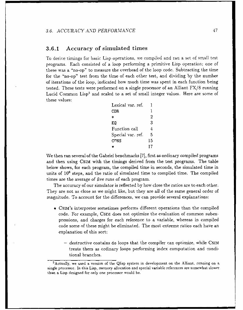
3.6. ACCURACY AND PERFORMANCE 47
3.6.1 Accuracy of simulated times
To derive timings for basic Lisp operations, we compiled and ran a set of small testprograms. Each consisted of a loop performing a primitive Lisp operation; one ofthese was a "no-op" to measure the overhead of the loop code. Subtracting the timefor the "no-op" test from the time of each other test, and dividing by the numberof iterations of the loop, indicated how much time was spent in each function beingtested. These tests were performed on a single processor of an Alliant FX/8 runningLucid Common Lisp 5 and scaled to a set of small integer values. Here are some ofthese values:
Lexical var. ref. 1CDR I+ 2EQ 3Function call 4Special var. ref. 5CnNS 15• 17
We then ran several of the Gabriel benchmarks [7], first as ordinary compiled programsand then using CSIM with the timings derived from the test programs. The tablebelow shows, for each program, the compiled time in seconds, the simulated time inunits of 106 steps, and the ratio of simulated time to compiled time. The compiledtimes are the average of five runs of each program.
The accuracy of our simulator is reflected by how close the ratios are to each other.They are not as close as we might like, but they are all of the same general order ofmagnitude. To account for the differences, we can provide several explanations:
* CSIM's interpreter sometimes performs different operations than the compiledcode. For example, CSIM does not optimize the evaluation of common subex-pressions, and charges for each reference to a variable, whereas in compiledcode some of these might be eliminated. The most extreme ratios each have anexplanation of this sort:
destructive contains do loops that the compiler can optimize, while CsIMtreats them as ordinary loops performing index computation and condi-tional branches.
5Actually, we used a version of the Qlisp system in development on the Alliant, running on asingle processor. In this Lisp, memory allocation and special variable references are somewhat slowerthan a Lisp designed for only one processor would be.

48 CHAPTER 3. A PARALLEL LISP SIMULATOR
- stak uses special variables, which are quite slow on the version of Lispthat we used. The compiled code uses deep binding, which takes a varyingamount of time per reference, while CsIM charges a constant amount oftime.
- taki does a lot of tail-recursive function calling, which is optimized by thecompiler.
Compiled SimulatedTime Time Ratio
boyer 22.06 27.74 1.3browse 19.63 41.02 2.1ctak 1.56 3.26 2.1dderiv 6.99 7.72 1.1deriv 5.96 7.15 1.2destructive 2.18 7.89 3.6div test-I 2.63 4.22 1.6div test-2 3.44 3.62 1.1stak 6.09 2.39 0.4tak 0.53 1.11 2.1takl 2.04 8.39 4.1takr 0.72 1.11 1.5
* CsIM pretends that garbage collection time is a constant multiple of the timespent in allocation functions, by including it in the cost of these functions.This is not accurate; a copying garbage collector takes time proportional tothe amount of memory in use when it is called, which may be large or smalldepending on the program being tested.
3.6.2 Speed of the simulator
Next we will compare the speed of CsIM itself with the speed of compiled code thatit is simulating. The computation of function timing statistics (see Section 3.2.6)was disabled during these tests; turning it on slows CsIM by an extra factor of 2 ormore. We also ran the programs through the Lucid Common Lisp interpreter forcomparison.
The times in the table below are all in seconds. The CSIM runtimes are the averageof three runs, except for boyer and browse which were only run once. The rundimes

3.6. ACCURACY AND PERFORMANCE 49
for interpreted and compiled code are the average of five runs.
CSI'm Interpreted CompiledRuntime Time Ratio Time Ratio
boyer 9441.32 1313.54 7.2 22.06 428browse 12125.03 1142.68 10.6 19.63 618ctak 488.61 94.65 5.2 1.56 313dderiv 1105.40 103.66 10.7 6.99 158deriv 1192.60 116.65 10.2 5.96 200destructive 2315.31 244.35 9.5 2.18 1062div test-1 1406.86 207.71 6.8 2.63 535div test-2 999.59 118.05 8.5 3.44 291stak 475.61 107.76 4.4 6.09 78tak 433.87 65.67 6.6 0.53 818taki 3230.16 582.13 5.5 2.04 1583takr 456.09 66.67 6.8 0.72 633
During these tests there was some variation in running conditions. Running time onthe Alliant generally increases when several programs are executing simultaneously.This is probably due to contention for the cache, which is shared between its proces-sors. This factor makes as much as a 10% difference, so the figures above should betaken as rough approximations.
In some of the tests there was a significant amount of garbage collection. Enoughmemory was allocated to l'nit the garbage collection to once every few seconds, butnot so much as to cause paging of the Lisp process.
CSIM generally took 300 to 1000 times as long as the compiled version of the codeit was interpreting, i.e., 5 to 15 minutes to simulate a second of compiled code.
The comparison with the Lucid interpreter shows much less variation in the speedratio, reflecting the fact that CsiM and an ordinary interpreter do similar things witha program. In general, CSIM is about 5 to 10 times slower than the interpreter, whichis a reasonable price to pay for the extra work that CsIM does to handle parallelprograms.
Both CsIM and the Lucid interpreter spend a lot of time doing storage allocationand garbage collection. The Lucid interpreter dynamically allocates lexical environ-ments just as CsIM does [31], but it uses a stack for dynamic binding and functioncalls. CsIM spends much of its time creating lexical closures for use as continuations.It runs best when given a lot of free storage, since this decreases the frequency ofgarbage collection. But the physical memory of the machine provides a limit to theamount of useful storage we can allocate; once this is exceeded and we start paging,performance drops tremendously.

50 CHAPTER 3. A PARALLEL LISP SIMULATOR
Although these tests simulated only one processor, they are indicative of thetimes that we get simulating parallel programs. since none of the code to manageconcurrency has been removed. The time to simulate a parallel program is roughlyproportional to the product of the number of processors we are simulating and theparallel runtime, with the same ratio as above, as long as most of the processors aredoing useful work. Simulating idle processors turns out to be more expensive thansimulating processors running ordinary code, because they are generally in a loopreferencing memory (checking a queue for work to do), and each such reference mustbe serialized as described in Section 3.4.1. We could probably modify CsIM to avoidthis source of inefficiency, but the difference does not seem worth the effort it wouldrequire.
3.7 A Parallel example
As an example of how CSIM is used, we will try to apply parallelism to the boyerbenchmark. Boyer [7, pp. 116-135] is a simple theorem prover that works by rewritinga formula into a canonical form (a structure of nested if-expressions), and thenapplying a tautology checker to the result.
Converting boyer to a parallel program is mainly an exercise; it is unlikely thatanyone will want to use the result. This is because there are better algorithms todo what boyer does, so it would pay to start from scratch and write a good paralleltheorem prover. Still, the case of parallelizing an existing sequential program is animportant one, and we expect to see it come up fairly often.
We begin with little knowledge of where the program spends its time. The firststep, therefore, is to simulate it running as a sequential program on one processor andlook at the function timing statistics (Section 3.2.6). Unfortunately, the benchmarkas given takes too much time and memory for easy experimentation; a single runthrough CSIM with statistics gathering turned on takes about 20 hours and causes alarge amount of paging. Therefore we will modify it to create a faster test.
The top level of the program is a function called test, which first constructs aterm by calling
(apply-subst(quote ((x f (plus (plus a b)
(plus c (zero))))(y f (times (times a b)
(plus c d)))(z f (reverse (append (append a b)
(nil))))
i i i I IIIIMI I I
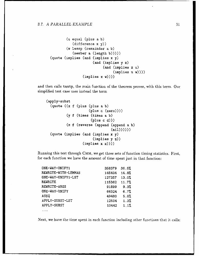
3.7. A PARALLEL EXAMPLE 51
(u equal (plus a b)(difference x y))
(w lessp (remainder a b)(member a (length b)))))
(quote (implies (and (implies x y)(and (implies y z)
(and (implies z u)
(implies u w))))(implies x w))))
and then calls tautp, the main function of the theorem prover, with this term. Oursimplified test case uses instead the term
(apply-subst(quote ((x f (plus (plus a b)
(plus c (zero))))
(y f (times (times a b)(plus c d)))
(z f (reverse (append (append a b)
(nil))))))(quote (implies (and (implies x y)
(implies y z))(implies x z))))
Running this test through CsIM, we get three sets of function timing statistics. First,for each function we have the amount of time spent just in that function:
ONE-WAY-UNIFY1 358379 36.5%REWRITE-WITH-LEMMAS 145404 14.8%ONE-WAY-UNIFYI-LST 127357 13.0%REWRITE 115362 11.7%REWRITE-ARGS 91899 9.3%ONE-WAY-UNIFY 66324 6.7%ASSQ 49480 5.0%APPLY-SUBST-LST 12504 1.3%APPLY-SUBST 10442 1.1%
Next, we have the time spent in each function including other functions that it calls:
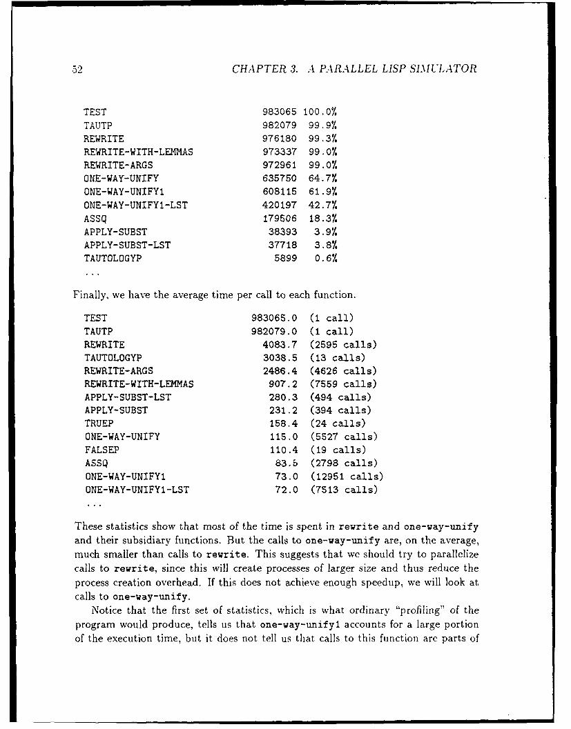
52 CHAPTER 3. A PARALLEL LISP SIMULATOR
TEST 983065 100.0%
TAUTP 982079 99.9%
REWRITE 976180 99.3%REWRITE-WITH-LEMMAS 973337 99.0%
REWRITE-ARGS 972961 99.0%ONE-WAY-UNIFY 635750 64.7%ONE-WAY-UNIFYI 608115 61.9%
ONE-WAY-UNIFY1-LST 420197 42.7%ASSQ 179506 18.3%APPLY-SUBST 38393 3.9%APPLY-SUBST-LST 37718 3.8%TAUTOLOGYP 5899 0.6%
Finally, we have the average time per call to each function.
TEST 983065.0 (1 call)TAUTP 982079.0 (1 call)REWRITE 4083.7 (2595 calls)TAUTOLOGYP 3038.5 (13 calls)
REWRITE-ARGS 2486.4 (4626 calls)REWRITE-WITH-LEMMAS 907.2 (7559 calls)APPLY-SUBST-LST 280.3 (494 calls)APPLY-SUBST 231.2 (394 calls)TRUEP 158.4 (24 calls)
ONE-WAY-UNIFY 115.0 (5527 calls)FALSEP 110.4 (19 calls)ASSQ 83.5 (2798 calls)
ONE-WAY-UNIFY1 73.0 (12951 calls)
ONE-WAY-UNIFYI-LST 72.0 (7513 calls)
These statistics show that most of the time is spent in rewrite and one-way-unifyand their subsidiary functions. But the calls to one-way-unify are, on the average,much smaller than calls to rewrite. This suggests that we should try to parallelizecalls to rewrite, since this will create processes of larger size and thus reduce theprocess creation overhead. If this does not achieve enough speedup, we will look atcalls to one-way-unify.
Notice that the first set of statistics, which is what ordinary "profiling" of theprogram would produce, tells us that one-way-unifyl accounts for a large portionof the execution time, but it does not tell us that calls to this function are parts of
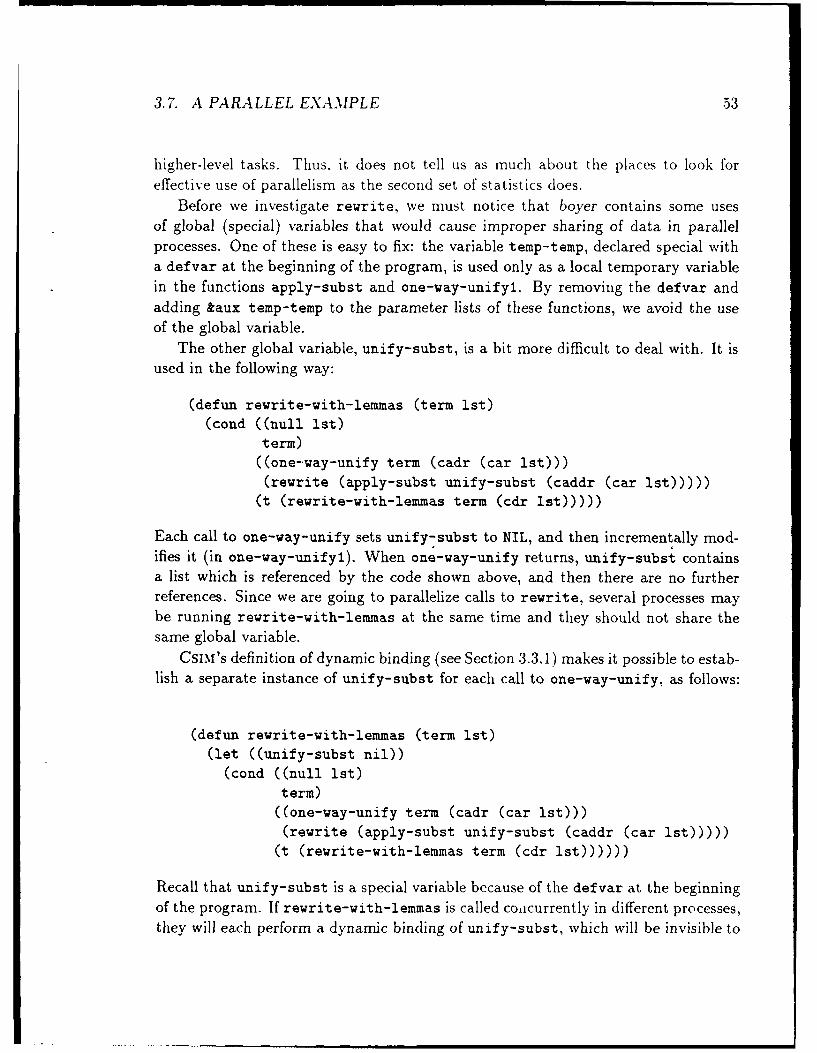
3.7. A PARALLEL EXAMPLE 53
higher-level tasks. Thus, it does not tell us as much about the places to look foreffective use of parallelism as the second set of statistics does.
Before we investigate rewrite, we must notice that boyer contains some usesof global (special) variables that would cause improper sharing of data in parallelprocesses. One of these is easy to fix: the variable temp-temp, declared special witha defvar at the beginning of the program, is used only as a local temporary variablein the functions apply-subst and one-way-unifyl. By removing the defvar andadding &aux temp-temp to the parameter lists of these functions, we avoid the useof the global variable.
The other global variable, unify-subst, is a bit more difficult to deal with. It isused in the following way:
(defun rewrite-with-lemmas (term lst)(cond ((null lst)
term)((one-way-unify term (cadr (car 1st)))(rewrite (apply-subst unify-subst (caddr (car lst)))))
(t (rewrite-with-lemmas term (cdr 1st)))))
Each call to one-way-unify sets unify-subst to NIL, and then incrementally mod-ifies it (in one-way-unifyl). When one-way-unify returns, unify-subst containsa list which is referenced by the code shown above, and then there are no furtherreferences. Since we are going to parallelize calls to rewrite, several processes maybe running rewrite-with-lemmas at the same time and they should not share thesame global variable.
CSIM's definition of dynamic binding (see Section 3.3.1) makes it possible to estab-lish a separate instance of unify-subst for each call to one-way-unify, as follows:
(defun rewrite-with-lemmas (term lst)(let ((unify-subst nil))(cond ((null 1st)
term)((one-way-unify term (cadr (car 1st)))(rewrite (apply-subst unify-subst (caddr (car 1st)))))(t (rewrite-with-lemmas term (cdr lst))))))
Recall that unify-subst is a special variable because of the defvar at the beginningof the program. If rewrite-with-lemmas is called coacurrently in different processes,they will each perform a dynamic binding of unify-subst, which will be invisible to
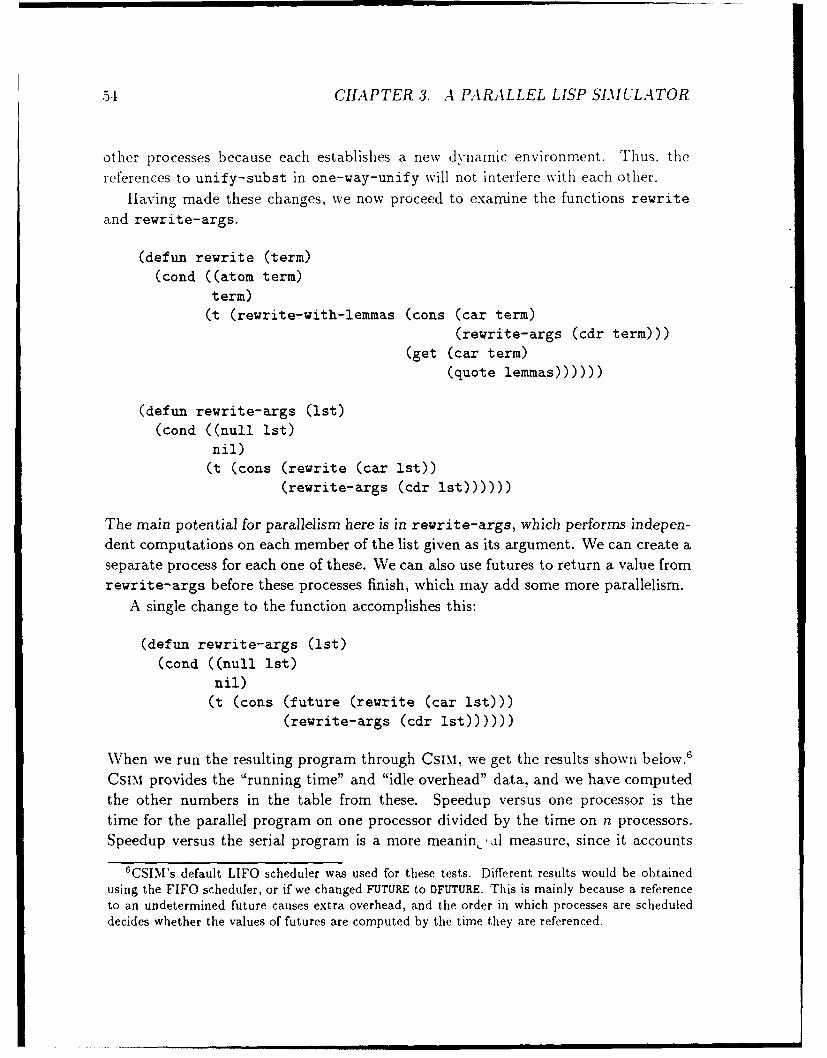
54 CHAPTER 3. A PARALLEL LISP SIMULATOR
other processes because each establishes a new dynamic environment. Thus. thereferences to unify-subst in one-way-unify will not interfere with each other.
Having made these changes, we now proceed to examine the functions rewriteand rewrite-args.
(defun rewrite (term)(cond ((atom term)
term)(t (rewrite-with-lemmas (cons (car term)
(rewrite-args (cdr term)))(get (car term)
(quote lemmas))))))
(defun rewrite-args (1st)(cond ((null ist)
nil)(t (cons (rewrite (car ist))
(rewrite-args (cdr 1st))))))
The main potential for parallelism here is in rewrite-args, which performs indepen-dent computations on each member of the list given as its argument. We can create aseparate process for each one of these. We can also use futures to return a value fromrewrite-args before these processes finish, which may add some more parallelism.
A single change to the function accomplishes this:
(defun rewrite-args (1st)(cond ((null ist)
nil)(t (cons (future (rewrite (car lst)))
(rewrite-args (cdr Ist))))))
When we run the resulting program through Csim, we get the results shown below.6
CsIM provides the "running time" and "idle overhead" data, and we have computedthe other numbers in the table from these. Speedup versus one processor is thetime for the parallel program on one processor divided by the time on n processors.Speedup versus the serial program is a more meanin, il measure, since it accounts
6CSI\I's default LIFO scheduler was used for these tests. Different results would be obtained
using the FIFO scheduler, or if we changed FUTURE to DFUTURE. This is mainly because a referenceto an undetermined future causes extra overhead, and the order in which processes are scheduleddecides whether the values of futures are computed by the time they are referenced.

3.7. A PARALLEL EXAMPLE 55
for overhead in the parallel program that we must try to avoid. The serial program'stime is 983065 steps, as computed in the earlier simulator run.
# of Running Speedup Speedup Useful Idle OtherProc. Time vs. 1 proc. vs. serial Work Overhead Overhead1 1367478 1.00 0.72 0.72 0.13 0.152 704366 1.94 1.40 0.70 0.15 0.153 491812 2.78 2.00 0.67 0.19 0.154 396999 3.44 2.48 0.62 0.22 0.165 346768 3.94 2.84 0.57 0.27 0.17
10 310896 4.40 3.16 0.32 0.50 0.1815 315602 4.33 3.12 0.21 0.63 0.1720 299398 4.57 3.28 0.16 0.68 0.15
The last three columns show the fractions of processor time spent doing useful workand overhead of various sorts. Useful work is the speedup vs. the serial time, dividedby the number of processors. This number stays well below 1.00 because of overheadin the parallel program. For each future, the parallel program does extra work tocreate the future, to add a process to the queue, to remove it when a processorbecomes idle, and to reference data indirectly through the future. The costs of futurecreation and adding processes are part of the "other overhead" above. The costs offinding processes in the queue and removing them are counted in "idle overhead."Idle overhead also counts time spent waiting for the lock on the queue, and timewhen there is no work for a processor to do.
Beyond about 10 processors, there is simply not enough work to keep all theprocessors busy, and the idle overhead begins to climb rapidly, while the "other over-head" fraction drops because the idle processors are not doing the operations thatare charged to that category.

56 CHAPTER 3. A PARALLEL LISP SIMULATOR

Chapter 4
Experimental results and analysis
In this chapter we present the results of experiments that compare the partitioningand scheduling methods described in Chapter 2, and analyze these results to explainwhat is happening and draw some general conclusions about the methods.
It is difficult to draw conclusions about the partitioning and scheduling methodswithout looking at specific examples of their use. Therefore, our approach is to beginwith experimental results on specific programs, explain them, and try to generalizethem to a larger class of programs.
4.1 The Fast Fourier Transform
The Fast Fourier Transform (FFT) is a computation with a very regular structure, andshould be easy to parallelize in any shared-memory programming model, even thoughits running time is only O(n log n) for input of size n. In addition to its applicationsin signal processing, the FFT is used as a subroutine in the fastest known algorithmsfor multiplying polynomials and large integers. This use of the FFT is the symbolicprocessing application we have in mind when choosing FFT as a test program.
Figure 4.1 shows a Common Lisp program for the Fast Fourier Transform.' Thisprogram differs in several ways from the more usual implemeptations.
* The basic structure of the program is recursive, not iterative. Each FFT of sizen performs two FFT's of size n/2 and merges the results. Changing from aniterative to a recursive program has a negligible effect on performance, and willallow us to add parallelism to the program more easily.
'The function cis called by the program computes cosO + isin0, returning a complex number.The symbol pi is the mathematical constant ,r. The function ash is an arithmetic shift, and is usedin several places to multiply and divide integers by 2. Using shifts instead of division turns out tomake a noticeable improvement in the program's performance.
57

CItAPTER 4. EXPERIMENTAL RESULTS AND ANALYSIS
ARRAY is the input array, of size ARRAY-SIZE. RESULT is theoutput array, of size RESULT-SIZE, which is the size of the FFTthat is performed. RESULT-SIZE must be a power of 2; ifARRAY-SIZE < RESULT-SIZE then ARRAX is considered to be paddedwith 0's.
(defun fft (array array-size result result-size)
(labels ((fft-inner (n r j m);; Store FFT of size N into RESULT starting at position;; R, using elements starting at position J in ARRAY with
;; step M.
(if (= n 1)(setf (aref result r)
(if (< j array-size) (aref array j) 0))(let ((n2 (ash n -1)))(fft-inner n2 r j (ash m 1))(fft-inner n2 (+ r n2) (+ j m) (ash m ))
(dotimes (k n2)(let ((x (aref result (+ r k)))
(y (* (aref result (+ r k n2))
(cis (/ (* -1 pi k) n2)))))
(setf (aref result (+ r k)) (+ x y))(setf (aref result (+ r k n2)) (- x y))))))))
(fft-inner result-size 0 0 1))
result)
Figure 4.1: The Fast Fourier Transform in Common Lisp
* The source and destination values are in different arrays. This arrangement ofthe data has several advantages over performing the FFT in place on Lhe inputarray: no shuffling (using bit-reversal) is necessary, and the input argument isnot modified, allowing its value to be reused. This version of the FFT algorithmcan therefore be used by a program written in a functional style. On the otherhand, we have decided to pass the output array as an argument to the fftfunction instead of having fft create and return a new array each time; thecaller of the function can then reuse an array when it is obviously safe to do so.An example of such reuse is when multiplying polynomials using the equation
a * b = FFT-1 (FFT(a). FFT(b)),

4.1. THE FAST FOURIER TRANSFORM 59
where *' denotes polynomial multiplication and '.' denotes term-by-term multi-plication. If the coefficients of the polynomials a and b are stored in the arrays Aand B, then we can allocate two new arrays T1 and T2, compute T +-- FFT(A):T2 + FFT(B); T, - T1 .T 2 ; and finally T2 +- FFT-1 (TI). (The inverse FFT isa slight variation of the FFT program. See [3] for a more detailed explanation.)
There are two sources of parallelism in the FFT program shown. The first is that therecursive calls to fft-inner may be performed in parallel, since they reference dif-ferent parts of the input and output arrays. Secondly, we can parallelize the dotimesloop in which pairs of input values are merged in a "butterfly" pattern. All of theiterations of the loop are independent and can be executed concurrently.
The recursive calls to fft-inner form a binary tree, and fit well into the heightcutoff and depth cutoff partitioning models that we have proposed. The computationdepth is easy to keep track of, and the height can be determined by looking at thesize of the subproblem being solved in the current call to fft-inner.
The height of a subcomputation is directly related to the value of the argument npassed to fft-inner. To implement a height cutoff, we replace the two calls tofft-inner by the form
(qlet (> n *height*)((xl (fft-inner n2 r j (ash m 1)))(x2 (fft-inner n2 (+ r n2) (+ j m) (ash m 1)))))
where *height* is a global variable that will contain the height cutoff value that wedecide to use. For a depth cutoff, we write
(let ((*depth* (1- *depth*)))(qlet (>= *depth* 0)
((xl (fft-inner n2 r j (ash m )))(x2 (fft-inner n2 (+ r n2) (+ j m) (ash m 1))))))
Here we are using Lisp's dynamic binding mechanism to give each process the ap-propriate value of *depth*. Before the top-level call to f ft, we set *depth* globallyto the number of levels in the tree that should cause processes to be created. \Vhen*depth* is rebound by the let expression, the effect is local to the process performingthe binding. This value is inherited by any subprocesses that are created, but whenthey reach the same let expression they will create new local bindings of *depth*,and so on. Thus each process uses the appropriate value in its partitioning test.
Note that in both of these versions of the parallel program, we use the qlet formto bind variables xl and x2, but never - their values. This is because the basicoperations of the program are side effects ,, an array.
• I I I Id

60 CHAPTER 4. EXPERIMENTAL RESULTS AND ANALYSIS
The dotimes loop in the original program does not immediately lend itself tothese methods. We could convert it to a loop that creates a process for each iteration.but then all of the potential processes would be the same size, and process creationoverhead might be too I igh to make any of them worthwhile. However, it is not hardto transform the loop irto code that recursively splits the range of indices in half ateach call, resulting in a binary tree of potential processes. These processes will varyin size just as the recursive calls to fft-inner do, and we will be able to apply heightor depth cutoff methods to this computation tree.
In our first experiment, we used height cutoff as the partitioning method andexamined four different scheduling methods. These are FIFO with a global processqueue, LIFO with a global queue, FIFO with a separate queue per processor, andLIFO with a separate queue per processor. We abbreviate these to FIFO, LIFO,FIFO* and LIFO*. Rather than try to guess a good height cutoff, we tested a widerange of values to see how the choice of cutoff value affects performance.
Figure 4.2 shows a selection of the results of this experiment. The most obviousthing to notice is the different performance of the various scheduling algorithms. Inall cases, LIFO* was the best-performing scheduler and FIFO the worst. The orderof the other two varied depending on the number of processors and height cutoff.The greatest differences in performance occurred at low values of the height cutoff,especially for the larger problem instances. Since there is such a clear winner amongthe schedulers, LIFO*, we will use it for the remainder of the FFT experiments.
In Section 2.3.1, we conjectured that the optimal height cutoff value would dependon both the number f processors and the problem size. The optimal depth cutoff,on the other hand, might be independent of the problem size. Figure 4.3 confirmsthe first prediction; in each graph, as the problem size increases the height cutoffgiving the best performance also increases. Also, the optimal cutoff varies for a givenproblem size n as we increase the number of processors p.
Figure 4.4 shows the corresponding curves when a depth cutoff is used. For somevalues of p, there is a single best cutoff value for all of the problem sizes o. In othercases, the optimal depth cutoff increases as n grows, though not as fast as the optimalheight cutoff did. It is much easier to choose a depth cutoff value that gives reasonablygood performance over the range of problem sizes tested. In particular, the optimalcutoff value for the largest n tested results in reasonably good performance over theentire range of problem sizes.
Our final set of graphs, in Figure 4.5, compares the "best" depth cutoff for eachvalue of p with the results of the dynamic partitioning method using a separate queueper processor, and creating a process only when this queue is empty. The dynamicmethod d.des not perform as well as the depth cutoff method for this range of problem
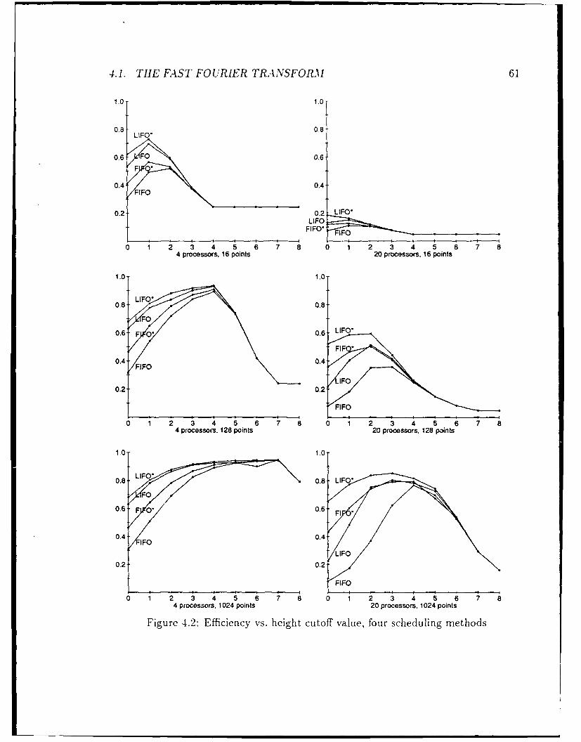
4.1. THE FAST FOURIER TRANSFORM I 61
1.0 1.0
0.8 0.8LIFO*
0.6 FO 0.6FO
0.4 0.4FIFO
0.2.2 LIFO*
LIFO
FIFO 'T i IFO
'.
0 1 2 3 4 5 6 7 8 0 1 2 3 4 5 6 7 8
4 processors, 16 points 20 processors, 16 points
1.0 ,.- 1.0
0.8 -0.8
0.6 - F0.6 LIFO-
0 1 2 3 4 5 6 7 8 0 1 2 3 4 5 6 7 8
4 processors 1024 points
20 processors, 1024 points
F.gu- 4.2:
E.s
0.8
0.80.2-
0.2
0 1 2 3 4 5 6 7 8 0 1 2 3 4 5 6 7 8
4 processors, 1 02 points
20 processors, 1 02 pointsFigur 4.2 E1fci nc vs eg t c t f u , o r s h d l n e h d
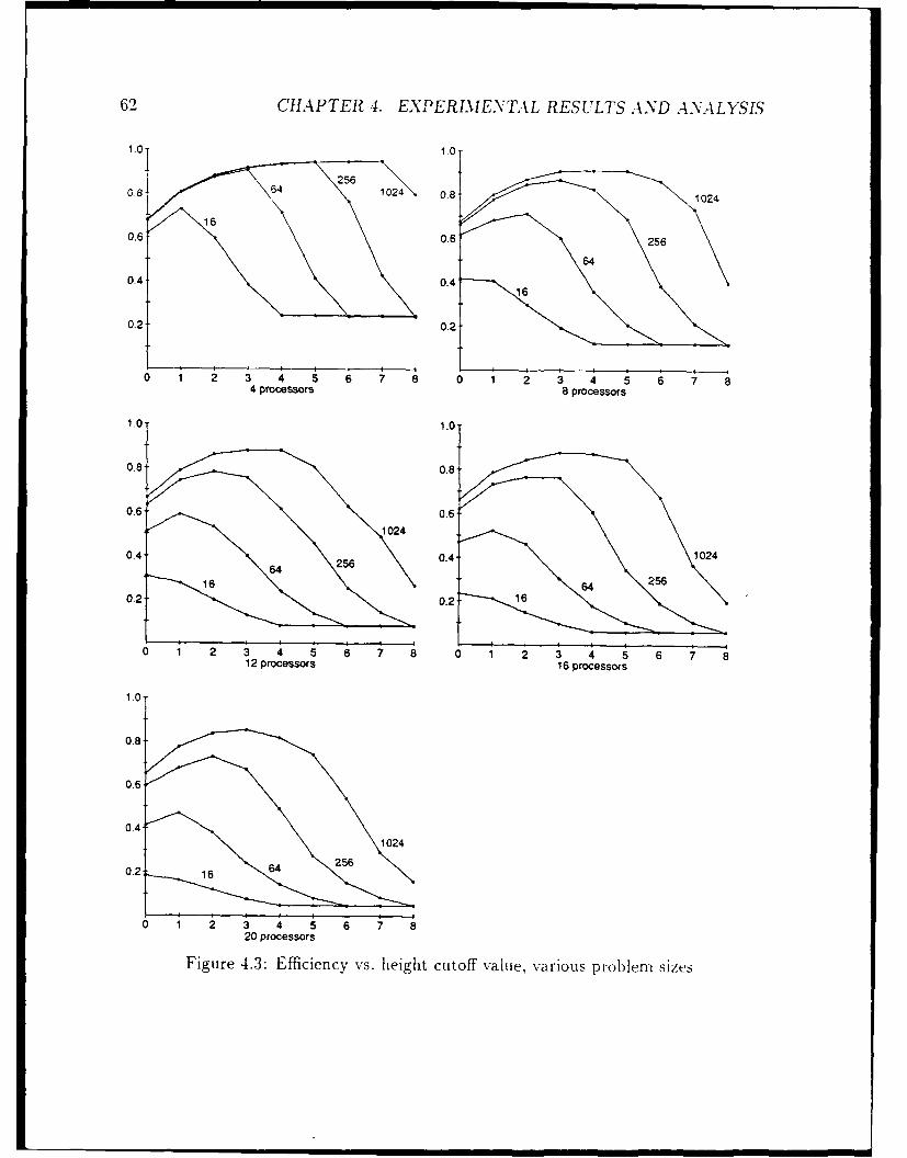
62 CHAPTER 4. EXPERIMENTAL RESUILTS AND A-NALYSIS
1.0 1.01
0.8 641024\ .8{12
0.2 .6r L
0.40.
0.2 162
0 1 2 3 4 5 6 7 8 0 1 2 3 4 5 6 720 processors 8poesr
Figur 4.3 Effcinc vs egtctf au, aiu be e
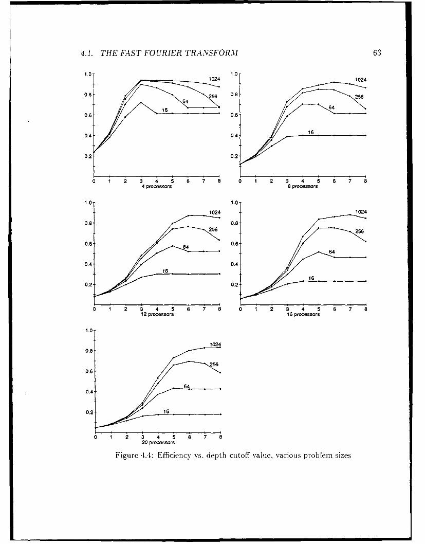
4.1. TE FAST FOURIER TRANSFORM 63
1.0 1.01024 1024
0.8 5 0.8
6040 .6
6456 .6
04 0.4 16
0 .2 , 0 .
0 1 2 3 4 5 6 7 8 0 1 2 3 4 5 6 7 84 processors 8 processors
1.0 1.0
1024 1024
0.8, 0.8
256 256
0.6 64 0.6
0.4 /!6
260.4
6 5
16
0.2 0.21r=
0 1 2 3 4 5 6 7 8 0 1 2 3 4 5 6 7 8
12 processors 16 processors
1.0 F
~1024
0.8"
0.4 64
0.2 1
0 1 2 3 4 5 6 7 820 processors
Figure 4.4: Efficiency vs. depth cutoff value, various problem sizes

64 CHAPTER 4. EXPERIMENTAL RESULTS AND ANALYSIS
1.0 dpth cutoff 1.0
0.8dynamic
0.6 -/ 0.6
16 64 256 1024 4096 16 64 256 1024 40964 processors 8 processors
1.0 1.0
0.8 0.8 depth cutoff
0.6 0.6
0.41. ,, dynamic 0.4t yai
0.2 0.2
16 64 256 1024 4096 16 64 256 1024 409612 processors 16 processors
1.0
0.8
0.6
0.40.2 dynamic
16 64 256 1024 409620 processors
Figure 4.5: Efficiency vs. problem size, for "optimal" depth cutoff and dynamic par-titioning
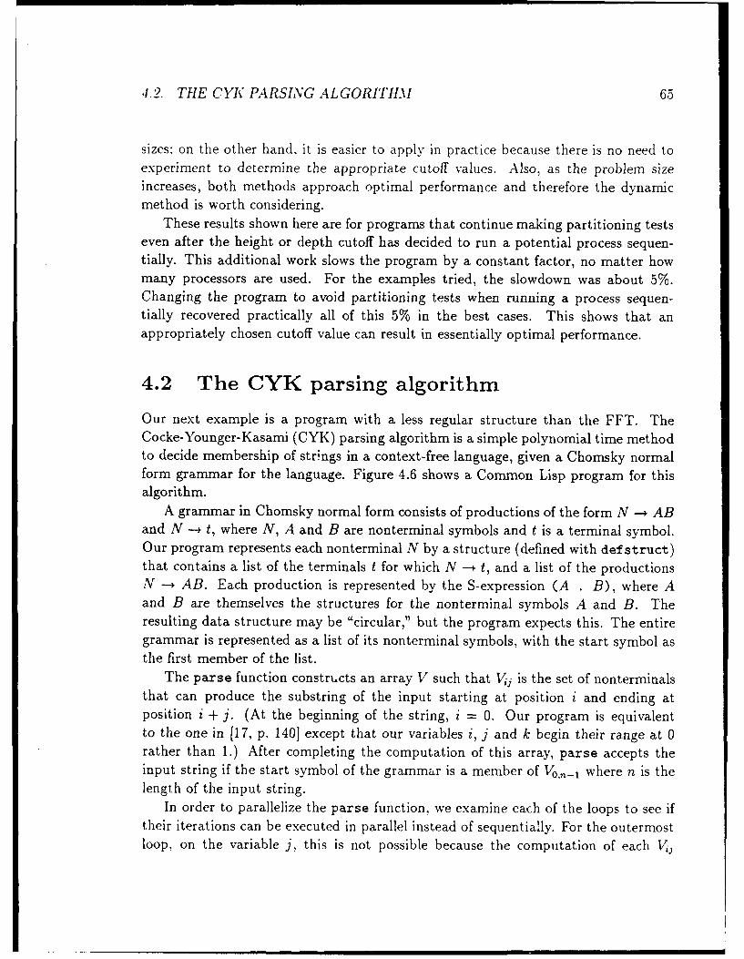
4.2. THE CYK PARSING ALGORITHM 65
sizes: on the other hand, it is easier to apply in practice because there is no need toexperiment to determine the appropriate cutoff values. Also, as the problem sizeincreases, both methods approach optimal performance and therefore the dynamicmethod is worth considering.
These results shown here are for programs that continue making partitioning testseven after the height or depth cutoff has decided to run a potential process sequen-tially. This additional work slows the program by a constant factor, no matter howmany processors are used. For the examples tried, the slowdown was about 5%.Changing the program to avoid partitioning tests when running a process sequen-tially recovered practically all of this 5% in the best cases. This shows that anappropriately chosen cutoff value can result in essentially optimal performance.
4.2 The CYK parsing algorithm
Our next example is a program with a less regular structure than the FFT. TheCocke-Younger-Kasami (CYK) parsing algorithm is a simple polynomial time methodto decide membership of strings in a context-free language, given a Chomsky normalform grammar for the language. Figure 4.6 shows a Common Lisp program for thisalgorithm.
A grammar in Chomsky normal form consists of productions of the form N -+ ABand N -+ t, where N, A and B are nonterminal symbols and t is a terminal symbol.Our program represents each nonterminal N by a structure (defined with defstruct)that contains a list of the terminals t for which N --* t, and a list of the productionsN -+ AB. Each production is represented by the S-expression (A . B), where Aand B are themselves the structures for the nonterminal symbols A and B. Theresulting data structure may be "circular," but the program expects this. The entiregrammar is represented as a list of its nonterminal symbols, with the start symbol asthe first member of the list.
The parse function constructs an array V such that Vii is the set of nonterminalsthat can produce the substring of the input starting at position i and ending atposition i + j. (At the beginning of the string, i = 0. Our program is equivalentto the one in [17, p. 140] except that our variables i, j and k begin their range at 0rather than 1.) After completing the computation of this array, parse accepts theinput string if the start symbol of the grammar is a member of V0,_ 1 where n is thelength of the input string.
In order to parallelize the parse function, we examine each of the loops to see iftheir iterations can be executed in parallel instead of sequentially. For the outermostloop, on the variable j, this is not possible because the computation of each V,

66 CHAPTER 4. EXPERIMENTAL RESULTS AND ANALYSIS
Grammar = list of nonterminals (beginning with start symbol)
Nonterminal = structure{ list of terminals t such that N -> t;
list of productions (A . B) such that N -> A B
(defstruct (nonterminal (:conc-name nil))
(terminals nil)
(productions nil))
(defun parse (str grammar)
(let* ((n (length str))(v (make-array (list n n) :initial-element nil)))
;; Initialization
(dotimes (i n) ;for i 0 to n-1
(let ((c (char str i)))
(dolist (a grammar)
(when (member c (terminals a))
(push a (aref v i 0))))))
;; Main loop
(do ((j 1 (1+ j))) ;for j 1 to n-1
((>= j n))(dotimes (i (- n j)) ;for i 0 to n-j-1(dotimes (k j) ;for k 0 to j-i
;; The body of this loop takes time bounded by a constant,
;; for any given grammar.
(let ((left (aref v i k))
(right (aref v (+ i k 1) (- j k 1))))(when (and left right)
(dolist (a grammar)(dolist (p (productions a))
(when (and (member (car p) left)
(member (cdr p) right))
(unless (member a (aref v i j))(push a (aref v i j)))))))))))
;; Test for acceptance.
(not (null (member (car grammar) (aref v 0 (1- n)))))))
Figure 4.6: The CYK parsing algorithm in Common Lisp

4.2. THE CYK PARSING ALGORITHM 67
depends on some of the values of Vy,j, with j' < j. The loops on i and k can beparallelized, however, since their iterations are completely independent.
Because parse performs assignments to shared memory, synchronization must beconsidered. The innermost loop performs the operation (push a (aref v i j)),creating a critical region of code. (The Common Lisp macro (push x y) is an abbre-viation for (setf y (cons x y)), which involves a read followed by a write to y.)Several processes doing this push concurrently with the same values of i and j wouldcreate a race condition, with the possibility of losing one of the pushed values if thereis no synchronization. If we only parallelize the i loop, there is no problem-any twoprocesses executing (push a (aref v i j)) will have different values of i. But ifwe parallelize the k loop, two processes with the same values of i and j may performconflicting push operations, so we must modify the program to synchronize these. Aswill be explained shortly, parallelizing both the i and k loops is necessary in order toget reasonable speedup.
Of the synchronization constructs discussed in Chapter 1, either locks, as providedby Multilisp, or process closures, as in Qlisp, are appropriate for this purpose. In ourexperiment we chose to use locks because the synchronization is at a very low level,and the overhead of process closures would slow down the program significantly. Giventhe choice between locks that loop while waiting for access to the critical region (spinlocks), or those that suspend the waiting process and resume it later, we chose spinlocks both to avoid overhead, and because we expect the delay in entering the criticalregion to be short most of the time.
The following new version of the inner loops in the program includes the necessarylocking constructs.
(dotimes (i (- n j)) ;for i 0 to n-j-1(let ((1 (make-lock)))(dotimes (k j) ;for k 0 to j-1
(let ((left (aref v i k))(right (aref v (+ i k 1) (- j k 1))))
(when (and left right)
(dolist (a grammar)
(dolist (p (productions a))(when (and (member (car p) left)
(member (cdr p) right))(get-lock 1)
(unless (member a (aref v i j))
(push a (aref v i J)))(release-lock l)))))))

68 CHAPTER 4. EXPERIMENTAL RESULTS AND ANALYSIS
Any processes that are created for the same value of i but different values of k willshare access to the lexical variable 1, and thus manipulate the same lock. Processesworking on different values of i will have different locks bound to the variable 1, sothere will be no unnecessary synchronization.
Modifying the program in this way to ensure correct behavior will necessarilyincrease its sequential runtime as well as its parallel runtime, because of the cost ofmanipulating the locks even if they never cause any processes to wait. Once we havedone this, we can not hope to achieve perfect speedup over the sequential runningtime. We will measure the sequential time of both the original program and theprogram with locks. The former should be used as the basis for reporting speedup,to provide an honest comparison of the sequential and parallel programs. The lattershould be used to decide when we have achieved a reasonable parallel running time,because it measures the work that is actually performed by the parallel program.
In the FFT example, the focus was on partitioning and scheduling strategies, be-cause identification of parallelism was fairly straightforward. In this program, findingsufficient parallelism is more difficult, and we concentrate on that. The experimentsabout to be described all used a single scheduling strategy-the LIFO* method thatshowed the best performance on FFT-and use variants of the dynamic partitioningstrategy.
The loops in parse have the same problem as those in FFT-the only concurrencythat is immediately available is to perform all of the iterations in parallel. A differencein this program is that the number of iterations of each loop varies, depending on thevalue of j in the outer loop. For small values of j, the loop on i has a large numberof iterations, each of which does a relatively small amount of work; while for large j,the i loop has a small number of iterations and each does a large amount of work.This is why parallelizing just the i loop is not sufficient; during the last few iterationsof the j loop, there will not be enough work to keep all of the processors busy.
Dynamic partitioning provides a useful means of resolving this problem. We allowall iterations of the i and k loops to define potential processes, and create an actualprocess only when the queue of work on the current processor is empty. As a point ofcomparison, we show what happens when just the i loop is parallelized in this way,to justify the claim in the previous paragraph.
Several versions of the CYK program were run. Input strings of sizes from 1to 20 were used, with three strings of each size chosen randomly and then used forall of the experiments. From 1 to 8 processors were simulated. The results shown arespeedups in relation to the serial code including locking, as mentioned above, so thebest possible value is not a true speedup of 8.0 but is the best that we can hope toachieve. The overhead for this locking was less than 5%, however, so the true speedup

4.2. THE CYK PARSING ALGORITHM 6988
6 6
4 4
2- 2-
2 4 6 8 1,0 12 14 16 18 20 2 4 6 8 10 12 14 16 18 202 processors 4 processors
8 8
6 6
4 4
2 2.
2 4 6 8 10 12 14 16 18 20 2 4 6 8 10 12 14 16 18 206 processors 8 processors
Figure 4.7: Speedup vs. problem size, parallelizing just the i loop
results do not differ much from what is shown.Figure 4.7 shows what happened when just the loop on i was parallelized. As
mentioned above, this does not create enough processes near the end of the compu-tation, so the poor performance that we see is understandable. Next, in Figure 4.8,we see the result of also parallelizing the loop on k. There is a slight improvement,but we are still far from approaching optimal speedup as we attained in the FFTexample.
We may ask whether the dynamic partitioning method is creating enough pro-cesses. To answer this question, we ran the program with all potential processescreated. Figure 4.9 shows the result of this version. On 2 and 4 processors, theperformance was slightly worse, due to the extra overhead, but on 6 and 8 processorsthe performance improved. This shows that there is potential for improvement overthe set of processes created by the dynamic partitioning method.
We next modified the dynamic partitioning method to create processes whenever

TO CHAPTER 4. EXPERIMENTAL RESULTS AND ANALYSIS81 8
61 6
4 4
2-2
2 4 6 8 10 12 14 16 1'8 2b 2 4 6 8 1'0 1'2 1'4 1'6 18 202 processors 4 processors
8 8
6. 6
4 4
22
2 4 6 8 10 12 14 16 18 20 2 4 6 8 1'0 1'2 1'4 1'6 18 206 processors 8 processors
Figure 4.8: Speedup vs. problem size, parallelizing both the i and k loops
the size of a processor's queue was less than 4, instead of less than 1 as we havedone so far. This will give more processes an opportunity to be created, while stillproviding a means to limit the amount of process creation. Figure 4.10 shows theresult of this experiment. There is some improvement over Figure 4.8, but we arestill far from optimal speedup.
With additional work, it may be possible to achieve better speedups for this pro-gram than those presented here, but we believe that the main obstacle to achievinggood speedup easily is the lack of parallelism at the highest level of the program (the jloop). The most promising approach to achieving further speedup is, therefore, elimi-nating this bottleneck. Making such a change to the program qualifies as redesigningthe algorithm. As we outlined at the beginning of Chapter 2, proper algorithm designis a vital part of achieving good parallel performance.
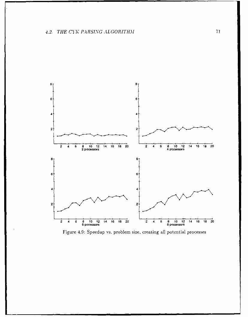
4.2. THE CYK PARSING ALGORITHI 71
8"8
6 6-
4 4-
2 2
2 4 6 8 10 12 14 16 18 20 2 4 6 8 10 12 14 16 18 202 processors 4 processors
88
6 6
4 4
2 2
2 4 6 8 10 12 14 16 18 20 2 4 6 8 10 12 14 16 18 20
6 processors 8 processors
Figure 4.9: Speedup vs. problem size, creating all potential processes

72 CHAPTER 4. EXPERLIENTAL RESULTS AND ANALYSISS
8 8
66
4- 4-
2 2
2 4 6 8 10 12 14 16 18 20 2 4 6 8 10 12 ;4 16 18 202 processors 4 processors
8 8
61 6
4 4
2-2
2 4 6 8 1'0 12 .'4 1'6 1'8 20 2 4 6 8 10 1,2 1,4 1,6 18 Zj
6 processors 8 processors
Figiire 4.10: Speedup vs. problem -ize, creating processes when queue length <

Chapter 5
Analysis of dynamic partitioning
In the experiments of the previous chapter, the performance of the dynamic parti-
tioning method was often close to that of the height and depth cutoff methods. This
is somewhat surprising, since the cutoff methods try to take advantage of knowledge
about the program, such as the expected size of processes, while the dynamic method
ignores such information.
This chapter examines the dynamic.partitioning method in more detail. In doingso, we will see some of the reasons why it is successful in spite of its fairly simple
approach to partitioning and scheduling.
5.1 Process creation behavior
We will analyze programs represented by computation trees, as described in Sec-
tion 2.1. These trees correspond to non-eager programs in which each potentialproess has at most one partitioning decision. To simplify the discussion, we make
the further assumption that at these partitioning points at most two subprocesses arecreated, i.e., the tree is binary. We will later extend these results to non-binary trees.
In Qlisp programs, these conditions restrict us to programs in which each potentialprocess executes at most one qiet form, and this qlet is of the non-eager variety
with (for the moment) two variable bindings. Two processes are created to evaluate
these expressions. Since, after creating these process s, the parent process will wait
for them to finish, the processor that was running the parent will immediately beginexecuting one of the two child processes. The other will remain in the processor'squeue.
The scheduling method that we initially analyze is the one where each processorhas a separate queue into which it adds processes that it creates, and from which it
73

74 CHAPTER 5. A.NALYSIS OF DYNAM.IIC PARTITIONING
removes processes when it is idle. If an idle processor's own queue is empty. it cycles
among the queues of other processors and will remove a process from one of those.At each partitioning decision, a processor checks to see if its own queue is empty.
If so, it creates the two subprocesses, putting one in the queue and running one itself,as described above. If the queue is non-empty, however, it does not create the newprocesses. Our assumption of binary computation trees implies that the queue willnever contain more than one process.
Suppose we are given a computation tree of height h satisfying the above as-sumptions, and execute it using our dynamic partitioning method on p processors.The computation starts with all queues empty and all processors idle, except for oneprocessor that is executing the topmost node of the tree.
Consider a processor that is idle at some point in the computation. It removesa process from either its own queue or the queue of another processor. This processis either a subtree of the original computation tree, or it is the continuation of aprocess that was suspended waiting for one of its children to finish. For now, let usjust consider the first case; later we will account for the resumption of suspendedprocesses.
When the execution of this process begins, the processor's queue will be empty,because we assumed the processor was previously idle. (If its queue was not emptywhen the processor became idle, we will have made it empty by removing the processthat was there-recall that there is never more than one process on a processor'squeue.) Therefore, the partitioning test in the topmost node of the tree will be true,and that node will create subprocesses for its children. Let us assume without loss ofgenerality that whenever a node creates subprocesses, it puts its right child tree ontoits queue and the processor continues with the evaluation of its left child.
As long as all of the processors are busy, the processes that they create are alladded to and removed from their own queues; none are taken from other processors'queues. This bounds the number of processes created as shown in the following
lemma.
Lemma 5.1 If a tree of height h is executed entirely on one processor, then O(h)processes are created during its execution.
Figure 5.1 shows the top part of a computation tree. Let h be the height of this tree.The processor that executes the root node of this tree will execute the entire tree. aslong as no other processor removes processes from its queue during the computation.In this case, the dark circles indicate those processes that decide to create subprocessesfor their children, and light circles mark those that do not. No processes are createdwhile the left child of the root node is evaluated, because the right child of the root

5.1. PROCESS CREATION BEHAVIOR 75
Figure 5.1: O(h) partitioning when there is no interference
(removed)
Figure 5.2: 0(h2 ) partitioning when there is interference
remains on the queue. When the processor finishes with the left child of the root andbecomes idle, it removes this process from its queue, and creates its right child processbecause the queue is now empty. Continuing in this way, it creates one process foreach level in the tree, for 0(h) process creations altogether. C
The rate of process creat")n can be higher when processors remove processes fromeach others' queues. For this case we show the following.
Lemma 5.2 IWhile a processor is executing a tree of height h, each time a process isremoved from its queue O(h2 ) processes are created.
Figure 5.2 shows what happens if another processor removes a process from the queuewhile a processor is evaluating a tree. In this example, the right child of the root

76 CHAPTER 5. ANALYSIS OF DYNAMIC PARTITIONING
node has been removed before the evaluation of the left half of the tree is finished.The arrow points to the next node that will make a partitioning decision. Since thequeue is now empty, a process is created, and (assuming this process is not removedby another processor) it will be executed on the original processor at its normaltime. When it finishes, however, the queue is again empty and the next partitioningdecision creates a process. The darkened nodes in the figure indicate the "cascade"of processes that is created as a result of the original right child's removal.
The cascade consists of a number of "branches," each of which starts one levelhigher in the tree than the previous branch, and extends down the right side of asubtree. When all of the work in such a subtree is finished, the program returns tothe parent node of the subtree, which has now finished its left child and begins workon its right child. At this point the processor's queue is empty, so 0(h) processes arecreated during the execution of the right child. There may be as many as h branches,leading to the 0(h 2) bound. 0
The removal of a process from the queue by another processor will be called a"transfer," to distinguish it from a processor removing a process from its own queue.
We will now derive an asymptotic upper bound on the total number of processescreated during the execution of a tree of height h. All subtrees of this tree haveheight less than h, so using h in place of the actual height of any subtree will stillgive an upper bound. Each tree that causes 0(h) process creations as described inLemma 5.1 must at some time have been transferred from another processor's queue,and thus causes O(h2 ) additional process creations. The 0(h 2 ) term dominates the0(h) term, so the total number of processes created is just 0(h 2 ) multiplied by thenumber of transfers. We now compute an upper bound for this quantity.
At any point during the computation, various subtrees of the original computationtree are unevaluated. These must all have height less than h, the height of the originaltree. Let H be the maximum height of any potential process that may still be createdin the remainder of the computation. H will decrease as the computation progressesand will be 0 at the end.
For each processor i, let Hi be the maximum height of any process that processori can create before becoming idle. (By "becoming idle," we mean finishing its currentprocess and any process on its queue.) Clearly Hi < H for each i, and H = max Hi,since all potential processes are part of a computation tree being executed or on thethe queue cf some processor. In order to reduce H by 1, we must reduce Hi by 1 ineach processor i for which Hi = H.
To illustrate using Figure 5.1, if the bottom level shown has height 1. then If, = 4after the process at the root node has created its children, because those children(whose height is 5) can create processes of height 4. During the evaluation of the
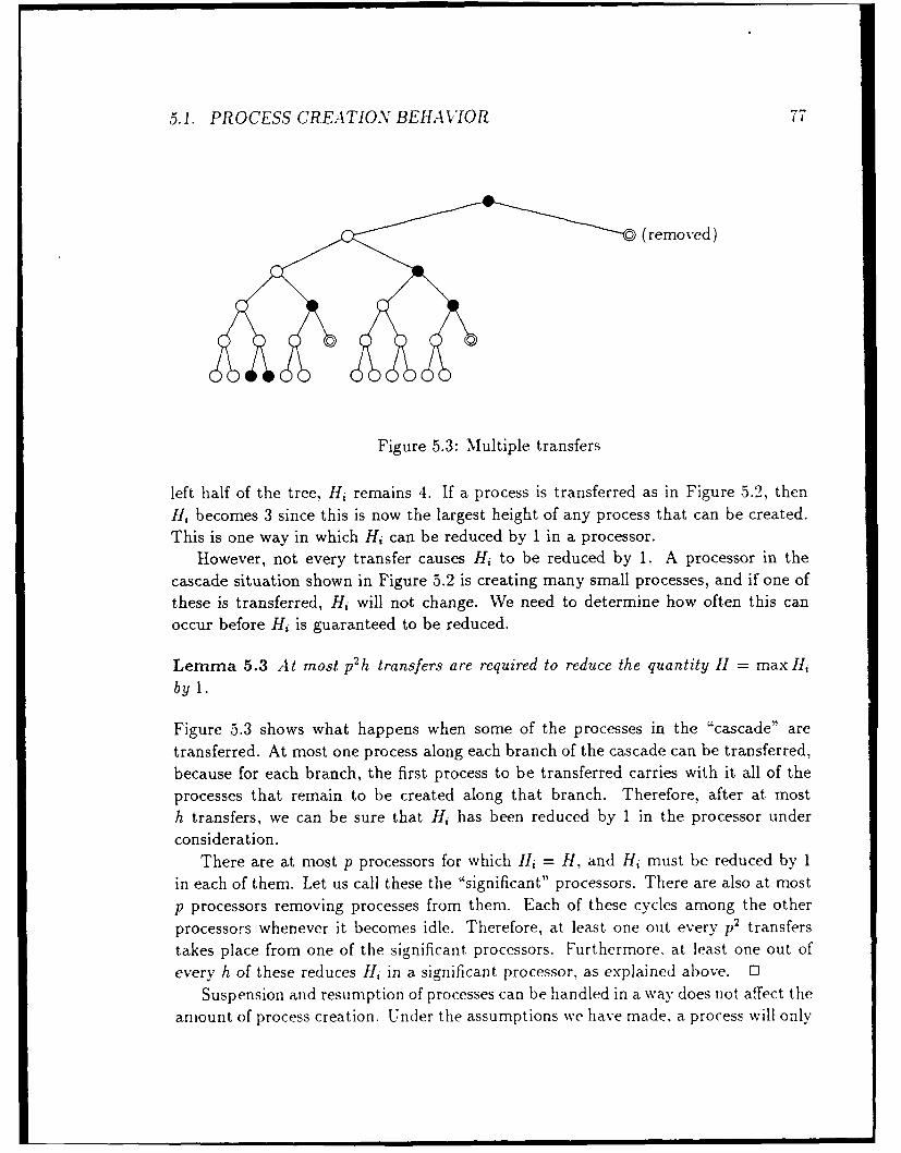
5.1. PROCESS CREATION BEHAVIOR 77
o (removed)
Figure 5.3: Multiple transfers
left half of the tree, Hi remains 4. If a process is transferred as in Figure 5.2, thenHi becomes 3 since this is now the largest height of any process that can be created.This is one way in which Hi can be reduced by 1 in a processor.
However, not every transfer causes Hi to be reduced by 1. A processor in thecascade situation shown in Figure 5.2 is creating many small processes, and if one ofthese is transferred, Hi will not change. We need to determine how often this canoccur before Hi is guaranteed to be reduced.
Lemma 5.3 At most p2h transfers are required to reduce the quantity H = maxH,-
by 1.
Figure 5.3 shows what happens when some of the processes in the "cascade" aretransferred. At most one process along each branch of the cascade can be transferred,because for each branch, the first process to be transferred carries with it all of theprocesses that remain to be created along that branch. Therefore, after at mosth transfers, we can be sure that Hi has been reduced by 1 in the processor underconsideration.
There are at most p processors for which Hi = H, and Hi must be reduced by 1in each of them. Let us call these the "significant" processors. There are also at most
p processors removing processes from them. Each of these cycles among the otherprocessors whenever it becomes idle. Therefore, at least one out every p2 transferstakes place from one of the significant processors. Furthermore. at least one out ofevery h of these reduces H, in a significant processor, as explained above. 0
Suspension and resumption of processes can be handled in a way does not affect theamount of process creation. Under the assumptions we have made, a process will only
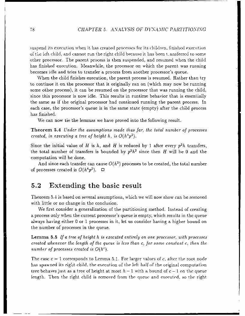
78 CHAPTER 5. ANALYSIS OF DYNAMIC PARTITIONING
suspend its execution when it has created processes for its children. finished executionof thie left child, and cannot run the right child because it has been t-ansferred to someother processor. The parent process is then suspended, and resumed when the childhas finished execution. Meanwhile, the processor on which the parent was runningbecomes idle and tries to transfer a process from another processor's queue.
When the child finishes execution, the parent process is resumed. Rather than tryto continue it on the processor that it originally ran on (which may now be runningsome other process), it can be resumed on the processor that was running the child,since this processor is now idle. This results in runtime behavior that is essentiallythe same as if the original processor had continued running the parent process. Ineach case, the processor's queue is in the same state (empty) after the child processhas finished.
We can now tie the lemmas we have proved into the following result.
Theorem 5.4 Under the assumptions made thus far, the total number of processescreated, in executing a tree of height h, is O(h4 p2 ).
Since the initial value of H is h, and H is reduced by 1 after every p2 h transfers,the total number of transfers is bounded by p2h2 since then H will be 0 and thecomputation will be done.
And since each transfer can cause O(h 2) processes to be created, the total numberof processes created is O(h4 p2 ). 0
5.2 Extending the basic result
Theorem 5.4 is based on several assumptions, which we will now show can be removedwith little or no change in the conclusion.
We first consider a generalization of the partitioning method. Instead of creatinga process only when the current processor's queue is empty, which results in the queuealways having either 0 or 1 processes in it, let us consider having a higher bound onthe number of processes in the queue.
Lemma 5.5 If a tree of height h is executed entirely on one processor, with processescreated whenever the length of the queue is less than c, for some constant c, then thenumber of processes created is 0(hc).
The case c = 1 corresponds to Lemma 5.1. For larger values of c, after the root nodehas spawned its right child, the execution of the left half of the original computationtree behaves just as a tree of height at most h - 1 with a bound of c - 1 on the queuelength. Then the right child is removed from the queue and executed, so the right

5.2. EXTENDING THE BASIC RESULT 79
half of the tree, whose height is at most h - 1, is executed with a bound of c on thequeue size. If S(c, h) is the maximum number of processes created for ally c and h,then
S(c, o) = 0S(O,h) = 0
S(c,h) = 1+ S(c- 1,h-1) + S(c,h-1)
The solution to this recurrence is the sum
which implies S(c, h) = O(hc). 13Lemma 5.2 is also affected when up to c processes can be present in each processor's
queue. If d of these processes are removed by other processors, then the processor inquestion can create a "cascade" of O(hd+1) new processes. The worst case, therefore,is when d = c and O(hc+l) processes can be created.
Theorem 5.6 If processes are created whenever the current size of the queue is lessthan c, then the total number of processes created in executing a tree of size h isO(hc+
3p2).
As in the proof of Theorem 5.4, at most p 2h2 processes are transferred altogether.Each of these causes O(hc+l) other processes to be created, and the product of thesefactors is the desired bound. As in Theorem 5.4, this term dominates the O(hc)processes that are created even if no processes are transferred. CD
We have also assumed that child processes are created just two at a time. Supposethat, instead, a program creates up to k processes at a time. The quantity k isconstant for any program, because the language constructs we are considering, suchas qiet, do not provide a way of creating a variable number of processes at one time.Such a program therefore corresponds to a computation tree in which each node hasat most k children.
The analysis of this situation depends on whether a single partitioning decision ismade once to create all k child processes or none; or if a separate decision is madefor each child process. The first of these situations is difficult to deal with, because ifwe create the children whenever the queue size is less than a constant c, we may endup with c + k - 1 processes in the queue, whereas our analysis assumed that thereare never more than c.
The second situation fits into the framework we have developed, however. If eacha node in the computation tree with k children is transformed into a binary tree with
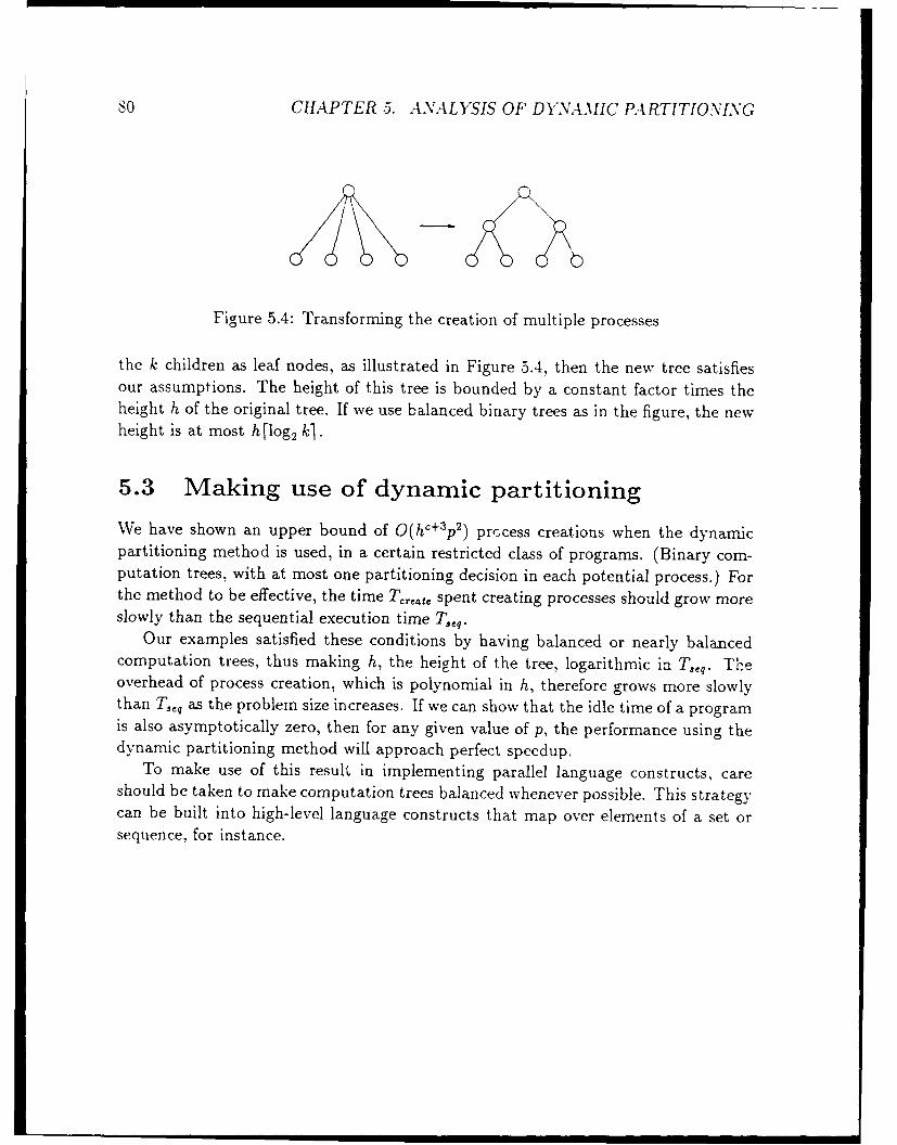
so CHAPTER 5. ANALYSIS OF DYNAMIC PARTITIONING
b
Figure 5.4: Transforming the creation of multiple processes
the k children as leaf nodes, as illustrated in Figure 5.4, then the new tree satisfiesour assumptions. The height of this tree is bounded by a constant factor times theheight h of the original tree. If we use balanced binary trees as in the figure, the newheight is at most h [log 2 ki.
5.3 Making use of dynamic partitioning
We have shown an upper bound of O(hc+3 p2) prccess creations when the dynamicpartitioning method is used, in a certain restricted class of programs. (Binary com-putation trees, with at most one partitioning decision in each potential process.) Forthe method to be effective, the time Tcreate spent creating processes should grow moreslowly than the sequential execution time Teq.
Our examples satisfied these conditions by having balanced or nearly balancedcomputation trees, thus making h, the height of the tree, logarithmic in Tq. Theoverhead of process creation, which is polynomial in h, therefore grows more slowlythan Tq as the problem size increases. If we can show that the idle time of a programis also asymptotically zero, then for any given value of p, the performance using thedynamic partitioning method will approach perfect speedup.
To make use of this result in implementing parallel language constructs, careshould be taken to make computation trees balanced whenever possible. This strategycan be built into high-level language constructs that map over elements of a set orsequence, for instance.

Chapter 6
Conclusions
We have examined the issues of partitioning and scheduling in parallel Lisp programsby examining several example programs, experimenting with different methods, andperforming an analysis of the dynamic partitioning method, because of its promisingcharacteristics.
The simulator that we wrote as part of this research proved very useful, sinceit allowed fine-grain observation of the effects of the programs that were studied,gave reproducible results, and had the ability to simulate more processors than werepresent on available parallel machines.
From a small number of example programs we cannot draw fully general conclu-sions, but we can make some observations based on the experience that has beengained. The first is that the cutoff-based partitioning methods are harder to applythan one might expect. The proper choice of a cutoff parameter depends on manycriteria, including the nature of the program, the size of the input data, and the num-ber of processors. Although it was possible to get rid of some of these dependencies,the selection of good cutoff values still required experimentation, and this is not thekind of work that we expect programmers will be willing to spend much time on.
Considering the amount of work needed just to get acceptable performance onour small programs, we believe that partitioning methods such as height or depthcutoff will prove almost totally impractical for large programs. A program thatperforms more complicated functions will undoubtedly have potential parallelism atmany points, and there may be complicated interactions when several sources of par-allelism are creating processes simultaneously.
The dynamic partitioning methni, on the other hand, is very appealing becauseit leaves the decision to create processes mostly to the system, but still bases iton information available at runtime, which we argued is necessary for satisfactoryperformance. Other projects in parallel Lisp have also come to this conclusion, but
81

82 CHAPTER 6. CONCLUSIONS
without performing a detailed analysis of the reasons for this method's strengths andlimitations. This analysis, we believe, is a useful contribution to the study of parallelprogram execution.
The analysis of dynamic partitioning can be extended in several ways.
1. We assumed that processes are always removed from the queue in the same way.In practice, better results have been observed when transferred processes areremoved from the head of another processor's queue (as in FIFO scheduling),while processes removed from a processor's own queue are run in LIFO order.
The reasons for this need to be explored.
2. When a process creates subprocesses at more than one point, our analysis doesnot apply. This kind of behavior occurs in many programs.
3. The average case behavior of dynamic partitioning, rather than the worst case, isof obvious interest. Preliminary experiments [22] show that, for some programsat least, the average-case behavior is proportional to the predicated worst-caseperformance, but the constant of proportionality is quite small.
4. Programs that use futures create a whole new realm of investigation. Otherparallel constructs such as the process closures and catch/throw extensions of
Qlisp also need to be analyzed.
At the end of the previous chapter we concluded that dynamic partitioning workswell with balanced computation trees, specifically those whose total size grows fasterthan a polynomial function of their height. This bears a resemblance to programsstudied in the theory of parallel computation. In that theory, the class NC of problemsthat can be done in polylogarithmic time on a polynomial number of processors isthought to be easy to parallelize. It might be possible to prove a relation betweenproblems in NC and programs that speed up well using the dynamic partitioning
method.Finally, our analysis of partitioning and scheduling methods helps define goals
for improved algorithms. The factor of p2 in our bounds on process creation meansthat the overhead on a given problem rises as we increase the size of the machine.We would be happier if the factor was p, meaning that the average rate of processcreation per processor is independent of the machine size. Perhaps some refinementsto the test used in dynamic partitioning will achieve this goal.
Bibliography
[1] Hal Abelson et al. The revised revised report on Scheme or an unCommonLisp. Al Memo 848, MIT Artificial Intelligence Laboratory, Cambridge., Mas-sachusetts, August 1985.
[2] Harold Abelson and Gerald Jay Sussman with Julie Sussman. Structure andInterpretation of Computer Programs. MIT Press. Cambridge. Massachusetts.1985.
[3] Alfred V. Aho, John E. Hopcroft, and Jeffrey D. Ullman. The Design andAnalysis of Computer Algorithms. Addison-Wesley, Reading, Massachusetts,1974.
[4] Thomas L. Anderson. The design of a multiprocessor development -ystem. Tech-nical Report TR-279, MIT Laboratory for Computer Science, Cambridge, Mas-sachusetts, September 1982.
[5] Isaac Dimitrovsky. ZLISP-A Portable Parallel LISP Environment. PhD thesis.New York University, New York, New York, March 1988.
[6] Daniel P. Friedman and David S. Wise. Aspects of applicative programming forparallel processing. IEEE Transactions on Computers, C-27(4):2s9-296, April1978.
[7] Richard P. Gabriel. Performance and Evaluation of Lisp Systems. ComputerSystems Series. MIT Press, Cambridge, Massachusetts, 1985.
[8] Richard P. Gabriel and John McCarthy. Queue-based multiprocessing Lisp. InConference Record of the 1984 ACM Symposium on Lisp and Functional Pro-gramming, pages 25-44, Austin, Texas, August 1984.
[9] Ron Goldman and Richard P. Gabriel. Qlisp: Parallel processing in Lisp. InProceedings of IIICSS-22, Hawaii International Conference on System Sciences,January 1989.
83

84 BIBLIOGRAPHY
[10] Michael J. C. Gordon. The Denotationa] Description of Programming Langniages.Springer-Verlag, New York, 1979.
[11] Allan Gottlieb, B. D. Lubachevsky, and Larry Rudolph. Basic techniques for theefficient coordination of very large numbers of cooperating sequential processors.ACM Transactions on Programming Languages and Systems, 5(2):164-189, April1983.
[12] Sharon L. Gray. Using futures to exploit parallelism in Lisp. Master's the-sis, Massachusetts Institute of Technology, Cambridge. Massachusetts, February1986.
[13] Robert H. Halstead, Jr. Multilisp: A language for concurrent symbolic computa-tion. ACM Transactions on Programming Languages and Systems, 7(4):501-538,October 1985.
[14] NV. Ludwell Harrison. Compiling Lisp for evaluation on a tightly coupled mul-tiprocessor. Technical Report 565, Center for Superccmputing Research andDevelopment, Urbana, Illinois, March 1986.
[15] Peter Henderson and James Morris, Jr. A lazy evaluator. In Conference Proceed-ings of the Third ACM Symposium on Principles of Programming Languages,pages 95-103, Atlanta, Georgia, January 1976.
[16] C. A. R. Hoare. Monitors: an operating system structuring concept. Communi-cations of the ACM, 17(10):549-557, October 1974.
[17] John E. Hopcroft and Jeffrey D. Ullman. Introduction to Automata Theory,Languages, and Computation. Addison-Wesley, Reading, Massachusetts, 1979.
[18] Takayasu Ito and Manabu Matsui. A parallel language PaiLisp and its kernelspecification. In Proceedings of the US/.Japan Workshop on Parallel Lisp, Sendai,Japan, June 1989.
[19] David Jefferson. Virtual time. ACM Transactions on Programming Languagesand Systems, 7(3), July 1985.
[20] John McCarthy et al. LISP 1.5 Programmer's Manual. MIT Press, Cambridge,Massachusetts, 1963.
[21] James S. Miller. MultiScheme: A Parallel Processing System Based on lITScheme. PhD thesis, Massachusetts Institute of Technology, Cambridge, Nias-sachusetts, August 1987.

BIBLIOGRAPHY 85
[22] Dan Pehoushek and Joseph S. Weening. 1989. Report in preparation.
[23] Vivek Sarkar. Partitioning and scheduling parallel programs for execution onmultiprocessors. Technical Report CSL-TR-87-328, Stanford University Com-puter Systems Laboratory, Stanford, California, April 1987.
[24] Guy L. Steele Jr. Common Lisp: The Language. Digital Press, Burlington,Massachusetts, 1984.
[25] Guy L. Steele Jr. and Gerald J. Sussman. LAMBDA: The ultimate impera-tive. AI Memo 353, MIT Artificial Intelligence Laboratory, Cambridge, Mas-sachusetts, March 1976.
[26] Guy L. Steele Jr. and Gerald J. Sussman. The revised report on SCHEME: A di-alect of LISP. Al Memo 452, MIT Artificial Intelligence Laboratory, Cambridge,Massachusetts, January 1978.
[27] Joseph E. Stoy. Denotational Semantics: The Scott-Strachey Approach to Pro-gramming Language Theory. MIT Press, Cambridge, Massachusetts, 1977.
f28] Pete Tinker and Morry Katz. Parallel execution of sequential scheme with para-tran. In Conference Record of the 1988 ACM Sympcsium on Lisp and FunctionalProgramming, pages 28-39, Snowbird, Utah, July 1988.
[29] Mitchell Wand. Continuation based multiprocessing. In (,.,iference Record ofthe 1980 LISP Conference, Stanford, California, August 1980.
[30] Alexander Wang. Exploiting parallelism in Lisp programs with side effects. Bach-elor's thesis, Massachusetts Institute of Technology, Cambridge, Massachusetts,May 1986.
[31] Jon L. White. Personal communication.