199200088278 1.0 version 2.0 revision history october 1985; edited by richard l. white may 1990;...
TRANSCRIPT

SPACETELESCOPESOENCE
u--_~INSTITUTE
- NASA -ct<- /~9 , 750
NASA-CR-18975019920008278
Hubble Space Telescope
High Speed Photollleter
Instrulllent Handbook
§ H1R~"\ 'i'1.U f~iu·'pvIL.IDI fir\ ~ lJ • !
AUG 1 7 1990
LANGLEY RESEARCH CEIlT(:fl1I BRARY NASA
HAMPlON, VIRGil"" •
Version 2.0
May 1990
https://ntrs.nasa.gov/search.jsp?R=19920008278 2018-05-30T14:52:10+00:00Z
Version 1.0Version 2.0
Revision History
October 1985; edited by Richard L. WhiteMay 1990; edited by Richard L. White
The Space Telescope Science Institute is operated by the Association of Universities forResearch in Astronomy, Inc., for the National Aeronautics and Space Administration.
':j. ./ :i. ~:.:.:;': '''.:.1 r:': ... :i. ():: I. i. ',: <.<:; (·:d"!
() J HI)!.... ('I \/
(;!;-·j··f .i. ')' (j. ,':; '? I::: :1:\: i:'(.'ITE::C::iLlF('{ ::;i() I::·:F'T:I:I::: !'·I(.:·I~::;I'·:·I·· CI:::·:l ;:Y·:.'i')':::'.;')() () .,/ I) I:.::.i / 0 () 1.'+ (:l F' (::1 C·:·) F: :::) 1....1 I'i c:::L (:I f; ;::) IF:' J F: D
1 ..iTTL.::
(\111 ii ::C;Cn:';:F' ::'::::(If> :1
C.:: J (J II
I'I() <.ii::) I:
1"1 I !\!U::
DiJC:i..i!'IL!\!Tr:;~(.:,.!\/ :'1. ·::::.C:'c:li' .j i..,l, 1::) Ll :1. ~.:::: ':3 r) :'::'( c: t·:·::: .~ {~::l 1(.::' :::: c: C'IJ -c.:.:':: i'''! i f~:,:.i }'''l '::::,,:) E'::l·::~IC! j:) j"'j t) '1:.: Cr ni('::::' '1.',: ~:,';:' s'" :'i. '('j';:::. t. 'f" U ITIC·:~1 "\"\ 'i,'; I"~} ,';;1, 'l"l (.I 1:) C,I C:l k ";::.::,,0('I': t·HI J IT: ,: F: T('!ii:'Ii{I) L." F'{YT:: P,./ f:::·:d "~~~;~:)ace "I"e:le~l~~(:::(::I~:)e Sc:::j,ey')(:::e ]:)"l~l~;'lu!l Ba:l'tj,111(::'¥"8:t 111:)"
!J \\1 If r:: D ':3 ..'" (\f E: U.':::~·!I (:i I'·! Dr:: i) lJI:: :::::; .i~: F' IICIT (J \"1 E:r I::: h: ::::; /i:: E;F' ('! C~ F:: I:: iJ r;: !\I 1:::: (i '::::;T F;: C! !I[! 1'1 \' ./:,~ LJ !.:::; C: i:;.; F: L: I.:! Ij I r:: E: Ii! L: I)'1:::::/ C:(iL.1 E(r:;.~(lf I I'·IF) i/ I·! I C;II HF'E:E:D/ iIC.!):·)I:·I!.... F: HF'(jC:E: ·11::::I....r:.. :::;)C:UF'!:::./ bE:I'!::::; l'f I \..1 1.1"/
{':f }:,'::,;~:::~ ~~ r! "j ':1. :::: if! .::} 'j'''I',J (':";! ]. :~, ';:;~ ~::·I. f,~J 1..,\ :'\. dE':': 'f' \) 1''' ~';:'l ';::;. '1:,: '1''' [, r'"i C) rii {,:.::: Y" '::::. i,:\ll"'l c' i Y"j "!:.:E:! 'j"',;.::\ '1:.: D Li '::::. ~:::':' '1:.: I"'I (::::1 1·,,1:i. \;:,l !"l i.::~' i:.:.::' clPhotometer (~18P), one of the scientific instruments onboard the Hubble:;:::;!J r'i:\ .:',:: (::~l l i\·:;; J E'::,' ';:E· Co, Cl tJ E·:' (1.. ·1 ~:3 ''I'') II (::'i], 1 t: !"'1 (~':' i '('I of () '(' fn ':;':"', 'i:.: i CI f'J 'I ", E~': C':~I cl E';' d ,,{ -t> y. c; f' cl :i. r'~ _;':';1, }" )/ U '::::. t·;::.' :::~ f) "{' t,: I"j (.:~.:\
HSP is presented, including: (1) an overview of the instrument; (2) a1:.:1 I,::' 1;:::,. :i. 1 c·:: cl ,:,:,i c.::' ':',: L:: '1''' i j:::' t. ::. c' '1'''1 [:'f ::,: C) me:.' d :::.,: t;. ':'::'. i I::::. 0 'ft:...! ("::' IF:) F' .... :;:::; ·f::::. '/ .:::,. '1:.: '::':', I'!'I t \''', .::..... t. if: ·:::t 'Ii' 1::)('.::,
i Hi F' () 'J'" t ~':;). 1'''1 t 'of D '(' ~:E D ffi (,:~:'l 0 !::) '::::, (,:.:,:1 Y" \/ {'::\ t,: i 0 r"} ';:::. H (~~~ ) t ;:~t i::) ]. {':.:':' ~:::' ,':':\ i"i d 'f i (,:,:J \J )'" {:{~, ~::;. d (~':'1 ~::; c: '(' i I:::, i 'n {.~.i t i'''i (~':'1
':::' iC.',) ii'::·::· :i.i;; :1. \/ ]. \':>, ""'1"1 cl 11 rn ':1 t:,::\ \:,: :'1. 0'("1'::.:· c,"f 'i;,: h (,.::, 1"\'.:::'::1"'.':, ( ,:+::. i', [, 1/\1 '1:.: c' IJ c' i::,b I.::' 1.. 1. '1:.: 1::.'I:i. ':':". ('1'1'''11 ·('IIJ:::".'I''',observation with the HUP; and (5) a description of the standard':::: :::' J !. I'J j'" :,:" I:.. '! c' '1", t. ::::' !::;; ~.:': .::':'I.!.') F' 1 :i. (.,::,;.::1 to I'! I:;:;; F' ci ,::". I:.: <,:, ·::Of. ';'''1 d t.I"·II",:: f' E~::::· i...! 1 t i i"'1 c.:.1 d ;::\ t i:':i F' (. [, d u c: t:::; "
E: !\i ''1'' E: F~ ::

HIGH SPEED PHOTOMETER INSTRUMENT HANDBOOK
Version 2.0
Richard L. White
Space Telescope Science Institute
3700 San Martin Drive, Baltimore, MD 21218

HSP Instrument Handbook Version 2.0
Table of Contents
Chapter 1: Introduction1.1 How to Use This Manual1.2 Acronyms . . . . . . .1.3 Acknowledgements ...
Chapter 2: Overview of the HSP2.1 Summary of HSP Characteristics2.2 Detectors and Optics Configurations
2.2.1 Single-Color Photometry2.2.2 Two-Color Photometry with Prisms2.2.3 Two-Color Photometry with the PMT2.2.4 Polarimetry . . . .2.2.5 Images with the HSP . . . . . . . .
2.3 Electronics .2.4 Mechanical Structure and Thermal Characteristics2.5 Observing with the HSP
2.5.1 Target Acquisition . . . . . . . . .2.5.2 Sky Subtraction Modes . . . . . . .2.5.3 Occultation Observations with the IISP2.5.4 Other Useful Information . . . . .
Chapter 3: Details of the HSP-ST System3.1 Internal Details of the IISP
3.1.1 The Bus Director3.1.2 Standard Data Formats
3.2 The HSP-ST System . . .3.2.1 Changing Filters with the HSP3.2.2 Limits to the Length of Uninterrupted Observations3.2.3 Unequally Spaced Data .....3.2.4 Absolute Timing of Observations .
3.3 Sources of Noise and Systematic Errors3.3.1 Noise . . . . . . . . . .3.3.2 Systematic Errors .....3.3.3 Reducing Systematic Errors
Chapter 4: Instrument Performance4.1 Sensitivity of the HSP .....4.2 Planning a Typical Observation with the HSP
4.2.1 How to Calculate Exposure Times4.2.2 Polarimetry of the Crab Pulsar ....
Chapter 5: Standard Calibrations and Data Products5.1 "Pipeline" Calibrations5.2 Data Products5.3 Special Calibrations
Chapter 6: Bibliography
11123334i'7I
910101313131516161818181819191920202121212224243838394141414243

ii
Tables
HSP Instrument Handbook Version 2.0
Table 1-1: Acronyms .Table 2-1: HSP Configurations and ModesTable 3-1: HSP Data Formats ..Table 4-1: HSP Photometry Filters .Table 4-2: HSP Polarimetry Filters .Table 4-3: HSP Beamsplitter FiltersTable 4-4: Locations of HSP FiltersTable 4-5: HSP Detectors . . . . .Table 4-6: Sky Background Counting Rates for I" AperturesTable 4-7: Target Acquisition Time (minutes) .
Figures
Figure 2-1: HSP Optics and Detectors .....Figure 2-2: HSP Focal Plane Layout . . . . .Figure 2-3: HSP Filter/Aperture Tube ConfigurationFigure 2-4: VIS IDT Apertures and FiltersFigure 2-5: UVI IDT Apertures and Filters . . . .Figure 2-6: UV2 IDT Apertures and Filters . . . .Figure 2-7: Polarimetry IDT (POL) Apertures and FiltersFigure 2-8: HSP Electronics Block DiagramFigure 4-1: HSP Filters: 1000-2500 AFigure 4-2: HSP Filters: 2000-3500 AFigure 4-3: HSP Filters: 2500-7500 AFigure 4-4: HSP Filters: PolarimetryFigure 4-5: HSP Beamsplitter Filters: ThroughputFigure 4-6: HSP Longpass Filters .Figure 4-7: HSP Detector Quantum EfficienciesFigure 4-8: HSP Prism Beamsplitter CharacteristicsFigure 4-9: HSP PMT Beamsplitter CharacteristicsFigure 4-10: HSP Polarizer Characteristics ....Figure 4-11: Reflectivity of ST and HSP Mirrors ..Figure 4-12: Time to Reach V=15 with S/N=100: UV FiltersFigure 4-13: Time to Reach V=15 with S/N=100: UV, VIS Filters 1Figure 4-14: Time to Reach V=15 with S/N=100: UV, VIS Filters 2Figure 4-15: Time to Reach V=15 with S/N=100: Polarimetry FiltersFigure 4-16: Time to Reach V=15 with S/N=100: Beamsplitter FiltersFigure 4-17: Time to Reach V=15 with S/N=100: Longpass Filters
. 2
. 41825262627282829
456889
10123030313132323333343435353636373738

HSP Instrument Handbook Version 2.0
Chapter 1: Introduction
1.1 How to Use This Manual
1
This manual is a guide for astronomers who intend to use the High Speed Photometer (HSP),one of the scientific instruments onboard the Hubble Space Telescope (ST). All the informationneeded for ordinary uses of the HSP is contained in this manual, including:
(1) an overview of the instrument (Chapter 2),
(2) a detailed description of some details of the HSP-ST system that may be importantfor some observations (Chapter 3),
(3) tables and figures describing the sensitivity and limitations of the HSP (Chapter 4),
(4) how to go about planning an observation with the HSP (Chapter 4), and
(5) a description of the standard calibrations to be applied to HSP data and the resultingdata products (Chapter 5).
An HSP neophyte should begin by reading Chapters 2 and 4 to get an overview of the instrument and what it can do. Chapter 4 also shows how to write a proposal requesting observing timeusing the HSP. Chapter 5 describes the data products received by the observer. Skimming throughChapter 3 will give some feeling for the complications which may arise.
The HSP sophisticate will refer mainly to Chapters 3 and 4, and may often find that thecareful construction of complicated observing programs is driven by the constraints described inChapter 3.
Some observing programs will inevitably require more detailed information about the HSPthan is given here. For example, it is possible to write special purpose programs for a microprocessor inside the HSP that controls observing sequences, but this manual does not contain enoughinformation to determine precisely what can and cannot be done with such programs. If you requiresuch detailed information, it is available either from the Space Telescope Science Institute or fromthe documents listed in the bibliography of this manual.
As time passes, there will undoubtedly be changes in this manual. Chapters 3 and 4 areespecially vulnerable to changing as our knowledge of the instrument improves. Consequently,users should be wary of using outdated versions of the manual.
Suggestions for improvements are welcome and should be addressed to the author.
1.2 Acronyms
Acronyms are a necessary, if often overused, aid in reducing the length of NASA documents.The following acronyms may rear their heads in this manual:

2
A/DBDCVZFGSFOCFOSGSFCGHRSHSPIDTNASANSSC-lODSOTAPADPMTRAMROMSCUMSTSDASSOGSSTSTScITAVTBDTDRSSuvWF/PC
HSP Instrument Handbook Version 2.0
Table 1-1: Acronyms
Analog to DigitalBus DirectorContinuous Viewing ZoneFine Guidance SystemFaint Object CameraFaint Object SpectrographGoddard Space Flight CenterGoddard High Resolution SpectrographHigh Speed PhotometerImage Dissector TubeNational Aeronautics and Space AdministrationNASA Standard Spacecraft ComputerOptical Detector SubsystemOptical Telescope AssemblyPulse Amplitude DiscriminatorPhotomultiplier TubeRandom Access MemoryRead-Only MemorySystem Controller User's ManualScience Data Analysis SystemScience Operations Ground SystemHubble Space TelescopeSpace Telescope Science InstituteTarget Acquisition and VerificationTo Be DeterminedTracking and Data Relay Satellite SystemUltravioletWide Field/Planetary Camera
1.3 Acknowledgements
The High Speed Photometer was designed and built at the University of Wisconsin by Robert C.Bless (Principal Investigator) with scientific guidance from the HSP Investigation Definition Team:Joseph F. Dolan, James 1. Elliott, Edward L. Robinson, and Wayne van Citters. Among thosemaking major contributions to the design, construction, and testing of the HSP were Evan Richards,Jeff Percival, Fred Best, Dave Birdsall, Gene Buchholtz, Scott Ellington, Don Finegan, Ed Hatter, Sally Laurent-Muehleisen, Matt Nelson, Bill Phillips, Jerry Sitzmann, Mark Slovak, ColleenTownsley, Andrea Tuffii, Mark Werner, Doug Whitely, and others, to whom I apologize for theiromission from this list.
Much useful criticism of the HSP Instrument Handbook was provided by Bob Bless, JoeDolan, Howard Bond, and Lisa Walter; however, any remaining problems are the responsibility ofthe author.

HSP Instrument Handbook Version 2.0 3
Chapter 2: Overview of the HSP
The High Speed Photometer (HSP) exploits the capabilities of the ST by making photometricmeasurements over visual and ultraviolet (UV) wavelengths at rates up to 105 Hz and by measuringvery low amplitude variability (especially for hotter stars in the UV). A secondary purpose of theinstrument is to measure linear polarization in the near UV. The IISP has several advantages oversimilar ground-based instruments:
(1) UV wavelength coverage.(2) Smaller apertures, permitting higher spatial resolution and reducing the sky back
ground.(3) No atmospheric absorption or scintillation, leading to higher photometric accuracy
and the ability to use very short sample times.
In what follows we will present an overview of the HSP, its optics and detectors, its electronics,its mechanical structure, and finally some observational considerations.
2.1 Summary of HSP Characteristics
Quantum Efficiency:Time Resolution:
Photometric Accuracy:Apertures:
Filters:Polarimetry:
Operation:
",0.3-3% (throughput for entire HSP-ST system)10.8 J.ls (pulse-counting mode, count rate < 106 cts/s)",1 ms (current mode, count rate> 106 cts/s)Systematic errors < 0.1% from V=O to V=200.4, 1.0 arcsec diameter for normal observations6.0, 10.0 arcsec for target acquisition23 UV and visual filters from 1200 A to 7500 A4 UV filters0.2% polarimetric accuracyTelescope must slew to move star from one filter to another.Slew time'" 30-60 s (limits rate at which multicolor photometry is possible). There are 4 filter pairs with beamsplitters which can be used for 2 color photometry withoutmoving telescope; for these filter pairs, can get simultaneousor nearly simultaneous (separated by only 10 milliseconds)2 color photometry.
2.2 Detectors and Optics Configurations
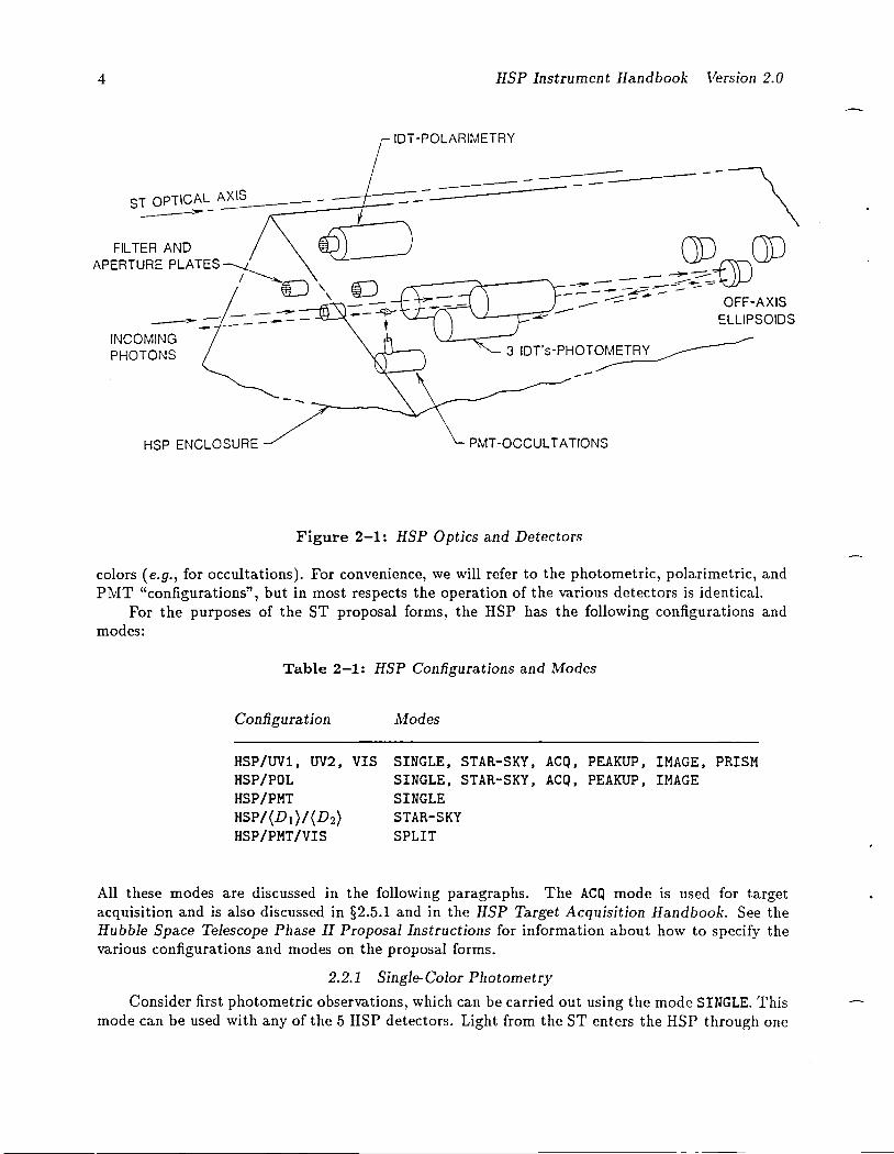
The IISP has quite an unusual design, in that it has no moving parts. Figure 2-1 shows asketch of the arrangement of the detectors and optics in the HSP. There are five detectors in theinstrument-four image dissector tubes (IDTs) and one photomultiplier tube. The former are ITT4012RP Vidissectors, two with CsTe photocathodes on MgF2 faceplates (sensitive from 1200 Ato 3000 A) and two with bialkali cathodes on suprasil faceplates (sensitive from 1600 A to about7000 A). Each image dissector tube, its voltage divider network, and its deflection and focus coils areall contained in a double magnetic shield within the housing. The photomultiplier is a HamamatsuR666S with a GaAs photocathode. Three of the image dissectors-the two CsTe tubes (calledUV1 and UV2) and one of the bialkali tubes (VIS)-are used for photometry. The second bialkalidissector (POL) is used for polarimetry,* and a beamsplitter allows the photomultiplier (PAIT)along with the bialkali photometry dissector (VIS) to be used for simultaneous observations in 2
* Note that the polarimeter also has 1 clear filter which can be used for photometry.
4 HSP Instrument Handbook Version 2.0
lOT-POLARIMETRY
ST OPTICAL A_X_\S __ :- - =_---J-FILTER AND
APERTURE PLATES~
I~U'
_-J_~_~- 'INCOMING 7--PHOTONS ~
--HSP ENCLOSURE PMT-OCCULTATIONS
Figure 2-1: HSP 0 pties and Detectors
colors (e.g., for occultations). For convenience, we will refer to the photometric, polarimetric, andPMT "configurations", but in most respects the operation of the various detectors is identical.
For the purposes of the ST proposal forms, the HSP has the following configurations andmodes:
Table 2-1: liSP Configurations and Modes
Configuration Modes
HSP/UV1, UV2, VISHSP/POLHSP/PMTHSP/(D 1)/(D2)HSP/PMT/VIS
SINGLE, STAR-SKY, ACQ, PEAKUP, IMAGE, PRISMSINGLE, STAR-SKY, ACQ, PEAKUP, IMAGESINGLESTAR-SKYSPLIT
All these modes are discussed in the following paragraphs. The ACQ mode is used for targetacquisition and is also discussed in §2.5.1 and in the HSP Target Acquisition Handbook. See theHubble Space Telescope Phase II Proposal Instructions for information about how to specify thevarious configurations and modes on the proposal forms.
2.2.1 Single-Color PllOtometry
Consider first photometric observations, which can be carried out using the mode SINGLE. Thismode can be used with any of the 5 HSP detectors. Light from the ST enters the HSP through one

HSP Instrument Handbook Version 2.0
tV3 (Y-axis)
5
V2-- X-axis-100 mm
10'
Focal Plane Layoutseen from behind focal plane)
HSP(As
Figure 2-2: HSP Focal Plane Layout
of three holes in its forward bulkhead. These holes are all centered on an arc 8.1 arc min off-axis;the focal plane layout for the HSP is shown in Figure 2-2. After passing through a filter (which isabout 36 mm in front of the ST focal plane) and an aperture (which is in the ST focal plane), thelight is brought to a refocus on the dissector photocathode by a relay mirror-a 60 mm diameteroff-axis ellipsoid located about 800 mm behind the ST focal surface. The relay mirrors enable amore efficient use to be made of the ST focal plane available to the HSP than would otherwise bepossible, i.e., the image dissectors are too large to place more than two directly in the focal plane.The magnification of the relay mirrors is about 0.65, which converts the f/24 bundle entering theHSP to {/15.6 at the photocathode, with a corresponding change in scale from 3.58 arcsec/mmto 5.54 arcsec/mm. The off-axis ellipsoids produce images at the photocathode which are about0.25 arcsec in diameter. The actual intensity distribution at each image is a combination of thegeometrical aberrations and the ST point spread function. Since about 70% of the energy in anST image 8 arcmin off-axis falls within a circle whose diameter is 0.2 arcsec, the total image blurwill be about V2 times larger than the geometric blur. For this reason, one set of HSP apertureswas made 0.4 arcsec in diameter. Images that encompass 90% or more of the energy, however, aremore than 0.5 arcsec in diameter. Addition of the effects of worst-case pointing jitter and otheruncertainties led to the choice of 1.0 arcsec for the diameter of the second set of apertures. The0.4 arcsec apertures will be used when the background light is important (e.g., for occultationsor for observations of very faint objects); the 1.0 arcsec apertures will be used when the greatestphotometric accuracy is desired.
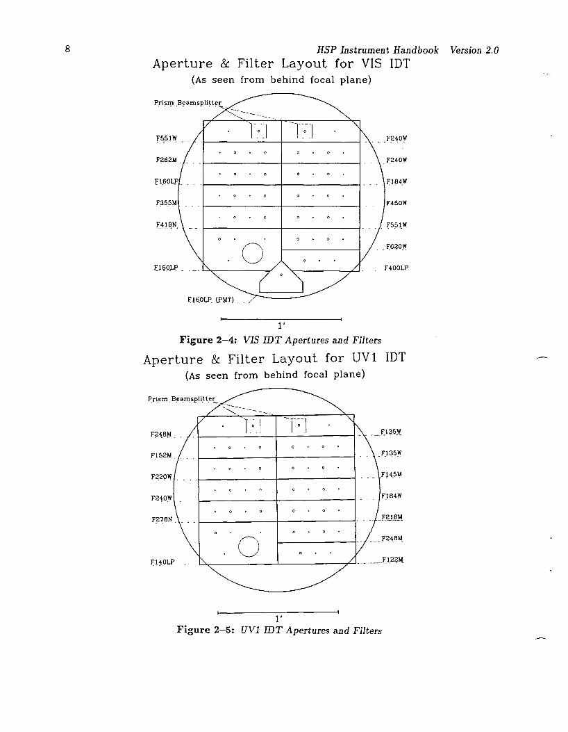
The only unusual feature of the HSP's optical system is its filter-aperture "mechanism" (seeFigures 2-3 through 2-7) mounted behind each forward bulkhead entrance hole. Each filter platecontains thirteen filters mounted in two columns positioned 36 mm ahead of the ST focal plane.At this location the converging bundle of light from the ST is 1.5 mm in diameter, well within the

6 HSP Instrument Handbook Version 2.0
/ RECEPTACLE
r"./Jv". /COVER
~~~
Figure 2-3: HSP Filter/Aperture Tube Configuration
3 mm width of each filter; however, since the light bundle is out of focus, small variations in filtertransmission with position should not be important. For each filter plate there is an aperture plate,located at the ST focal surface, which contains 48 apertures arranged in two columns that arepositioned directly behind the corresponding columns of filters. Nine of the filters are associatedwith four apertures each-two with diameters of 1 arcsec (280 pm) and two with diameters of 0.4arcsec (112 pm). Due to space limitations, one filter is associated with only three apertures, andtwo other filters are associated with two apertures each. The thirteenth filter, of double width, isa clear window and has five associated apertures, including one of 10 arcsec diameter for objectacquisition. The VIS detector has one additional aperture which also passes light to the PMT (see§2.2.3).
The ST is commanded to point so that the object's position in the ST focal plane coincideswith the particular filter-aperture combination desired. Light from the object is then focused onthe dissector cathode by the relay mirror. The resulting photoelectrons are magnetically focusedand deflected in the forward section of the image dissector so that the photocurrent is directedthrough a 180 pm aperture (corresponding to 1 arcsec on the sky). This aperture connects theforward section of the detector to a 12-stage photomultiplier section. Thus with no moving parts,48 different filter-aperture combinations are available for each photometry detector in the HSP.Not all of these are unique, however, because of duplicate filters and duplicate apertures associatedwith each filter.
All of the UV filters are multi-layer interference filters of Al and MgF2 evaporated on MgF2substrates for the far ultraviolet, or on suprasil for the near UV. The visual filters consist of Ag andcryolite layers deposited on glass. The substrates are 1/16 inch (±0.002 inch) thick. The generalfilter characteristics are listed below in Tables 4-1 and 4-2. Some filters are common to two or morephotometry image dissectors for the sake of redundancy and to enable all three channels to be tied

HSP Instrument Handbook Version 2.0 7
together photometrically. Other filters define bandpasses similar to those flown on previous spaceobservatories, while yet others are similar to some in the Wide Field and Faint Object Cameras.
There is one filter on the POL IDT (F160LP, see Fig. 2-7) with two 0.65 arcsecond apertureswhich can be used for photometry. The other filters on POL have polarizers and can be used onlyfor polarimetry (§2.2.4).
Figure 2-2 shows the X and Y reference axes that are used if it is necessary to specify aparticular orientation for an HSP observation (using the ORIENT special requirement) ora specialposition for a target in an aperture (using the pas TARG special requirement). For example, theacceptable range of orientations may be restricted to insure that an aperture to be used for measurement of the sky brightness will not be contaminated by field star. (See §2.5.2 for discussion ofsky subtraction using the HSP.)
Notice that filter changes generally require the ST to slew from one aperture to another;this requires about 30 seconds for two apertures on the same IDT and about 60 seconds for twoapertures on different IDTs. The slew time determines how rapidly multicolor photometry can bedone. There are two exceptions to this restriction: rapid two-color observations can be made eitherin PRISM mode with detectors VIS, UVl, and UV2, or in SPLIT mode using PMT and VIS.
2.2.2 Two-Color Photometry with Prisms
On each photometry IDT, there is a beamsplitter/prism combination which divides the lightof an appropriately placed target between two 1 arcsec apertures which have different filters (seeFigures 2-4 through 2-6). A partially reflecting MgF2 plate mounted at 45° to the incoming beamtransmits part of the incident light to a filter and 1 arcsec aperture. The reflected beam is totallyinternally reflected by a right angle prism made of suprasil; it then passes through another filter, asuprasil rod (which compensates for the longer path followed by the reflected beam), and another1 arcsec aperture. In all cases, the transmitted beam passes through the short wavelength filterand the reflected beam goes through the long wavelength filter of the pair.
Using this prism beamsplitter (mode PRISM on the proposal forms), it is possible to measurean object's brightness in 2 colors merely by moving the IDT beam from one aperture to the otherrather than by slewing the ST, permitting observations in the two bandpasses separated by onlyabout 10 milliseconds rather than by the thirty seconds required for an ST slew. Thus, the prismspermit nearly simultaneous observations in two colors.
Only one pair of filters on each of the 3 photometry IDTs can be used with a prism; Table 4-3lists the 3 pairs of prism filters. Duplicates of all prism filters are also available as normal (straightthrough) filters without the intervening prism.
2.2.3 Two-Color Photometry with the PMT
In the SPLIT mode, light from the target object passes through a filter (in this case clearsuprasil, Fig. 2-4) and on through a 1 arcsec aperture, after which it strikes a Ag-Cryolite beamsplitter at 45° to the incident beam. The mirror reflects red light to the photomultiplier (PMT)via a red glass filter and a FabrY'lens. The beamsplitter passes a spectral band in the blue on toa relay mirror and to the VIS image dissector. Truly simultaneous observations can therefore bemade at about 7500 A and 3200 A.
The PMT detector and the F320N filter on the VIS detector can also be used independentlyfor single-color photometry (§2.2.1). However, there is ordinarily no advantage in doing so becausetaking data through both filters requires no additional observing time or overhead.
Note that the 45° reflection in both the PMT beamsplitter and the prism beamsplitters introduces significant instrumental polarization in the transmitted beam, so that the count rates for a10% polarized source will vary by about 2% with the ST roll angle.
8 HSP Instrument Handbook Version 2.0
Aperture & Filter Layout for VIS IDT(As seen from behind focal plane)
F450W
.1':620\,/
. j0184_W
. . F240W
.. F400LP
1-------+--------.,.... f5f>I_W
F355M
f~5rt! __.
f1.60Lp _ ..
~I!?OJ.]J _ . _ ~:-- ,.,
FI6_0I,.P_ {P~TJ. ./~----
l'
Figure 2-4: VIS IDT Apertures and Filters
Aperture & Filter Layout for UVl IDT(As seen from behind focal plane)
F248M1.;J -r~-J
Fl52M F.1 35\'i
F~20W F145~
F240W F.1 84W
F~~8N _.. - J~~.M
0 .___ f~4.8M.
. ___fJ.2?M.jOl~OLP
l'Figure 2-5: UVl IDT Apertures and Filters

HSP Instrument Handbook Version 2.0
Aperture & Filter Layout for UV2 IDT(As seen from behind focal plane)
9
-....
F~62M1~ '!
F)45M
FI B1W F179M
F21BM Fl6QLP
F24BM F27BN
F?B4~
,~ - -F!45~
UF140LP F122!J
1'Figure 2-6: UV2 IDT Apertures and Filters
2.2.4 Polarimetry
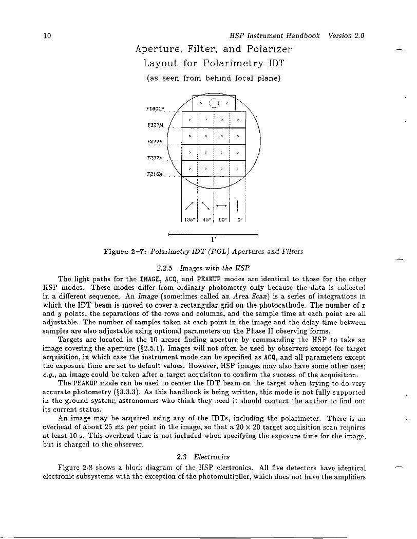
In the HSP/POL configuration, light from the target passes through a filter-aperture assembly(which is only about 4 arc min off-axis) directly to the image dissector; no relay mirror is used.The filter assembly (Figure 2-7) contains four near UV filters (see Table 4-2) across which are fourstrips of 3M Polacoat with polarizing axes oriented at 0°, 45°, 90°, and 135°. The aperture platecontains a single aperture for each filter-polarizer combination. There is also a clear window withtwo small apertures, which can be used for photometry, and a 6 arcsec diameter finding aperture.Linear polarization for a particular bandpass is measured by deriving the Stokes parameters Q andU from observations through each of the four polaroids in succession.
The internal IDT aperture for the polarimetric IDT is 180 /-Lm in diameter, the same as for thephotometric IDTs; however, because there is no relay mirror to change the plate scale, this corresponds to 0.65 arcsec on the sky. Thus, the internal aperture is slightly smaller than the 1 arcsecfocal plane apertures, and the effective aperture diameter for the polarimeter is 0.65 arcsec. Thisshould not affect the accuracy of polarimetry because the ST image is smaller at the polarimeterapertures due to the smaller astigmatism near the optical axis. However, it should be consideredwhen calculating the flux expected from extended sources.
For some observations, the polarimeter on the Faint Object Spectrograph might be betterthan that on the HSP. For example, the FOS would usually be preferable for a source which hasa polarized continuum contaminated by unpolarized line emission. On the other hand, the FOSpolarimeter may not be as well-calibrated as the HSP polarimeter during the initial phases of theST mission. See the FOS Instrument Handbook for details on the FOS polarimeter. Observersplanning to do polarimetry are encouraged to contact the STScI for advice on which instrument isbest for their proposal.
10 HSP Instrument Handbook Version 2.0
Aperture, Filter, and Polarizer
Layout for Polarimetry IDT
(as seen from behind focal plane)
0: o. 0
F16.0LP
f216M.
o () c
o : 0 • 0
1'
Figure 2-7: Polarimetry IDT (POL) Apertures and Filters
2.2.5 Images with the HSP
The light paths for the IMAGE, ACQ, and PEAKUP modes are identical to those for the otherHSP modes. These modes differ from ordinary photometry only because the data is collectedin a different sequence. An Image (sometimes called an Area Scan) is a series of integrations inwhich the IDT beam is moved to cover a rectangular grid on the photocathode. The number of xand y points, the separations of the rows and columns, and the sample time at each point are alladjustable. The number of samples taken at each point in the image and the delay time betweensamples are also adjustable using optional parameters on the Phase II observing forms.
Targets are located in the 10 arcsec finding aperture by commanding the HSP to take animage covering the aperture (§2.5.1). Images will not often be used by observers except for targetacquisition, in which case the instrument mode can be specified as ACQ, and all parameters exceptthe exposure time are set to default values. However, HSP images may also have some other uses;e.g., an image could be taken after a target acquisiton to confirm the success of the acquisition.
The PEAKUP mode can be used to center the IDT beam on the target when trying to do veryaccurate photometry (§3.3.3). As this handbook is being written, this mode is not fully supportedin the ground system; astronomers who think they need it should contact the author to find outits current status.
An image may be acquired using any of the IDTs, including the polarimeter. There is anoverhead of about 25 ms per point in the image, so that a 20 X 20 target acquisition scan requiresat least 10 s. This overhead time is not included when specifying the exposure time for the image,but is charged to the observer.
2.3 Electronics
Figure 2-8 shows a block diagram of the HSP electronics. All five detectors have identicalelectronic subsystems with the exception of the photomultiplier, which does not have the amplifiers
HSP Instrument Handbook Version 2.0 11
needed in the image dissectors to drive focus and deflection coils. The x and y deflections and focussettings are 12-bit programmable quantities. A change of 1 in the deflection corresponds to a beammotion of about 4 J.lm (0.02 arcsec). The high voltage power supplies are 8-bit programmable toprovide negative DC voltages between 1400 and 2600 volts for the detectors.
The settings of all internal HSP quantities will usually be handled automatically by STScI,although there may be rare observations that require changing the high voltage, discriminatorsettings, etc., to get the best performance from the HSP.
The output of the detectors can be measured by counting pulses, by measuring the photocurrent, or by doing both simultaneously. In the current (analog) data format*, a current-to-voltageconverter measures detector current outputs over a range of 1 nA to 10 J.lA full scale in 5 decadegain settings selectable by discrete command inputs. The amplifier output is converted to a 12-bitdigital value by an A/D converter. The analog data format will be used for stars that are too brightfor the pulse-counting data formats. One benefit of the programmability of the high voltage is thatit provides a means of extending the dynamic range of the detectors in their analog data format.The minimum sample time in the analog data format is set by the analog-to-digital conversiontime of 128 J.lS. The true time resolution in analog data format is somewhat larger than this; itis determined by the time constant of the current amplifier, which ranges from 4 ms in the 1 nArange to 0.4 ms in the 10 J.lA range.
It should be emphasized that the effective integration time when collecting data with theanalog format is always very short. For example even if the sample time is specified to be 1 sec, theeffective integration time is only "",1 ms. Thus, decreasing the sampling rate leads to widely spaced,short samples of the brightness of the star, but does not increase the accuracy of measurementfor each sample. The number of samples required to achieve a specified accuracy using the analogformat is essentially independent of the sample time (and may be very large for faint objects).
In the pulse-counting (digital) data format, the output of the preamplifiers, which provide avoltage gain of about 7, is received by pulse amplifier/discriminators (PADs). The PADs amplifyand detect pulses above a threshold set by an 8-bit binary control input, enabling the signal-to-noiseratio to be optimized for any high voltage setting. The PAD thresholds are usually set by STScIand will rarely be of concern to the observer. Digital format data can be taken with sample timesas short as 10.8 J.lS. Pulses separated by about 40 ns or more can be separately detected so thatcount rates of up to 2.5 X 10⁵ Hz can be accommodated with a dead-time correction of no morethan one percent.
The sample times for both digital and analog data formats are commandable in 1 J.lS intervalsup to 16.384 s. Between successive samples there can be a delay time of zero to "'" 16 s, again in1 J1.s steps. This delay time will usually be set to zero except in cases where a delay is necessary forsome reason (e.g., in I-detector STAR-SKY mode, see below). Use optional parameters SAMPLE-TIMEand DELAY-TIME to specify these values on the exposure logsheet. By default the sample time is1 second and the delay time is its minimum possible value.
The five identical detector controllers perform those functions that relate to a specific detector,i.e., they receive a sequence of parameters and instructions from the system controller necessary foran observation and science data collection. Each contains an I/O port, a storage latch, two 24-bitpulse counters, and a multiplexer. Detector parameters are received from the system controllerthrough the I/O port and are stored in eight one-byte latches. These latch outputs are used tocontrol focus and deflection amplifiers, high voltage power supplies, discriminator thresholds, analoggain settings, etc. A 1.024 MHz clock signal, received through the I/O port, supplies a signal to theA/D converter and synchronizes sampling start and stop control signals to the two pulse counters.It can also be used as a test input to the counters. The outputs of the two pulse counters, the A/D
* For a detailed description of data format selections, see §3.1.2.

TEST CONN
SIGNAl CONi A
SIGNAL CONN B
POWER CONN A
POWER CONN B
HSP IIF CONNECTORS
Ct.«lS/SER '"CLQCI(S
ANLOIBttVl TIM
CMOS/SER TMCLOCKS
ANLO/BILVL TIM
POWER CONVERTER&
DISTRIBUTIONSl8SYSTEM
r--------------,I II II II II SYSTEM CONTROlLER A I
I II II I
DETECTOR POWER {
'''EfFACE SYSTE" CONT POWER {HEATERS HVPS POWER (5)~-,I,,,,-B j
DETECTORCONTROLLER
lIUlf'+-'-----..f-'~3-+-- -----jOOS HEATERS
TEST LAMPS
<p<p
IIIIII DEtECTOAI CONTROllERI
_________________ J IIII
r - - - - - - - - - - - - - - -"'J.< - - - - - - - - - - - - -- - ---,~ ~~ ~E~E:~~~~:.N~S__2__* ~~~T~R_E~E:T~O~I:.S~~S:.M~L~ ! _Jo----..,
~ ;~;;~~[~~O~~~~~~~~_~;~~~~~-~~~~~~~~~~~~;3; ~:---~=:±=~fJ~~iJ~~E~$~~~~====~S"~,'I'~,:A.B~~~~nL~~D~T~C':~ ~~~~~S_ ~ _ -.t+t-O~T:~~ :L~C~R~C~ ~S~~B~Y _ 4_ ....o------J ::
I I H-"""""-----jI DETECTOR ELECTRONICS ASSEMBLY S II r------------------, II I I SYSTEM CONTROLLER BI II I
I
L J
________________ __ .J
OPTICAL DETECTOR SUBSYSTEM,-----------------------1lOT DETECTOR A$$EfeL Y 1 I DETECTOR ElECTRONICS ASSEMBLY ,
r-----------------, I r------------------,I I I I
I
OfA BEA" -+--;--,!~t!':11G

HSP Instrument Handbook Version 2.0 13
converter, and the eight one-byte latches are multiplexed and transmitted through the detectorcontroller bus I/O port to the system controller.
As its name implies, the system controller's functions have to do with the instrument as awhole rather than with a specific detector. These functions include serial command decodingand distribution, detector controller programming, science data acquisition and formatting, serialdigital engineering data acquisition and formatting, and interfacing with the ST command anddata handling system through redundant remote modules and redundant science data interfaces.The system controller consists of an Intel 8080 microprocessor, memory, and various I/O ports.Direct memory access is provided to allow rapid data transfer through the science and engineeringdata ports and to allow science data acquired from the detector controllers to be stored in memoryquickly. An 8K byte ROM block is provided for the microprocessor program storage. The remainingmemory is composed of six 4K blocks of RAM which may be configured in any order. 4K of theRAM are allocated for the microprocessor system, 16K as a buffer for science data storage, and4K as a spare block. The spare block may be used to replace any other 4K block that becomesdefective. In contrast to the detector controllers, the system controller is dual standby redundant.
The power converter and distribution system converts the input +28V DC bus power from theST to secondary DC outputs required by all other subsystems and provides power input switchingand load switching for independent operation of individual detector electronics and heaters. TheDC-DC converters essential to overall instrument operation are dual standby redundant. Convertersthat power electronics associated with only one detector are not redundant. With three detectorsand their electronics on simultaneously the power consumption is about 135 W.
2.4 Mechanical Structure and Thermal Characteristics
The HSP is aligned and supported in the ST at three registration points. Two of these (oneforward and one aft) have ball-in-socket fittings, and the third point (in the forward bulkhead)provides tangential (rotational) restraint. The mechanical loads (including a pre-load to keep theHSP in alignment) are transmitted from the instrument to the telescope structure through thethree registration points. The two ball-in-socket fittings, the electronics boxes, and the optical anddetector system are all mounted directly to a box beam and baseplate, the main structural elementsof the HSP. The box beam runs the length of the instrument thereby connecting the two forwardand aft fittings and carries the pre-load. The baseplate (actually a milled-out lattice structure) isattached to the box beam and provides stiffness to the structure. Four internal bulkheads on eachside of the box-beam and baseplate form ten bays for the electronic boxes, which are mounted onthe baseplate. In addition to giving mechanical support to the electronics and to the wire harness,the baseplate provides a high conductance path between electronic modules as well as a radiatingsurface. The optics and detectors are mounted to (but thermally isolated from) the box-beam onthe side opposite the baseplate, and at the forward end of the instrument.
Detectors are not actively cooled and are expected to range in temperature between -15°Cand O°C for "cold" and "hot" orbits, respectively. Over an orbit their temperatures will change byno more than O.l°C. One consequence of the changing temperatures is that the IISP flexes slightly,causing the images of apertures to move on the faceplates of those IDTs that have relay mirrors(i.e., for all the IDTs except the polarimeter). The image motion is about 1 arcsec over the entiretemperature range. It is anticipated that the STScI will be able to compensate for this motion sothat it will not ordinarily be of concern to the observer.
2.5 Observing with the HSP
2.5.1 Target Acquisition
An observation with the HSP begins with the acquisition of the target. As for most of theother ST instruments, the IISP has 4 target acquisition strategies: Blind, Onboard, Interactive,

14 HSP Instrument Handbook Version 2.0
and Early. These schemes are described in detail in the HSP Target Acquisition Handbook; thissection briefly summarizes that document.
In a Blind target acquisition, the target is put directly in the desired 1.0 or 0.4 arcsec aperture.This is equivalent to doing no acquisition at all. However, it usually will be necessary to determinethe target position before going to a small aperture. Neither the target position nor the guide starpositions will generally be known accurately enough for a Blind acquisition except when the targethas been observed previously.
For the other target acquisition methods, the ST will acquire guide stars in such a way thatthe program star falls within the large finding aperture of the specified image dissector. The findingaperture has a diameter of 10 arcsec for the photometry IDTs and 6 arcsec for the polarimetry IDT.Nominal guide star and target positions should be accurate enough that the target will never falloutside the finding aperture. A 20 X 20 raster scan covering the finding aperture is then performedby the dissector to form a pseudo-image (the Acquisition image). Acquisitions are requested onthe proposal forms with the ACQ mode and must be listed as separate exposures on the exposurelogsheet. The type of acquisition must be specified using the ONBOARD (or INTERACTIVE or EARLY)ACQ FOR (lines) special requirement. Typical times required to collect the target acquisition imageare given in Table 4-7.
If the star field is simple so that the program star is easily identifiable, the target may hesuitable for an Onboard target acquisition. Software in the ST computer examines the pseudoimage and makes a list of up to 20 objects within a specified brightness range. The program starcan be specified to be the only candidate on the list (in which case it is an error if there is morethan one candidate) or the n-th brightest star on the list, where n is 1, 2, etc. The centroidlocation of the selected star is then found automatically and the correct telescope offset to thedesired filter-aperture is calculated. This offset is passed to the ST pointing control system and thesmall maneuver is carried out. The program star is now in the correct aperture with the detectorparameters properly set, and the observation begins.
If the program star is in a crowded field or is highly variable, it may not be possible to acquire itby means of the automatic finding routine described above. Instead, an Interactive or Early targetacquisition is necessary. In an Interactive acquisition, the psuedo-image is displayed on the groundwhere the observer indicates the program object with a cursor; then its position is transmitted toST. Obviously the observer must be present at the STScI if an Interactive acquisition is necessary.At most 20% of all observations will be allowed to have Interactive target acquisitions because oflimitations in communication links with the satellite.
In many cases the target acquisition image can be taken in advance of the actual observation(an Early acquisition), making real-time interaction with ST unnecessary. This avoids both thenecessity that the observer be present for the observations and difficulties with real-time interactionswith ST. Early acquisitions may also make use of the imaging instruments onboard ST, the WF fPCand the FOC.* If the field is very complicated, the target faint, or the target's ultraviolet magnitudevery uncertain, then it may prove useful (or necessary) to get a Wide Field Camera image of thefield before the HSP observation. ,The pointing requirements for target acquisition by the WF fPCare obviously much less stringent than those of the HSP. Unfortunately, the long slews required tomove a target from the WF fPC to the HSP will often preclude the use of the same guide stars forthe two instruments; this will mean that it will still be necessary to perform some sort of targetacquisition with the HSP before observing the target, though it may be possible to use a nearbystar which is suitable for an Onboard acquisition. See the Target Acquisition Handbooks for theHSP and the other instruments for more information on various strategies for difficult cases.
* The FOC will not be used as often as the WF fPC because its field of view is only twice thediameter of the HSP finding apertures.
HSP Instrument Handbook Version 2.0 15
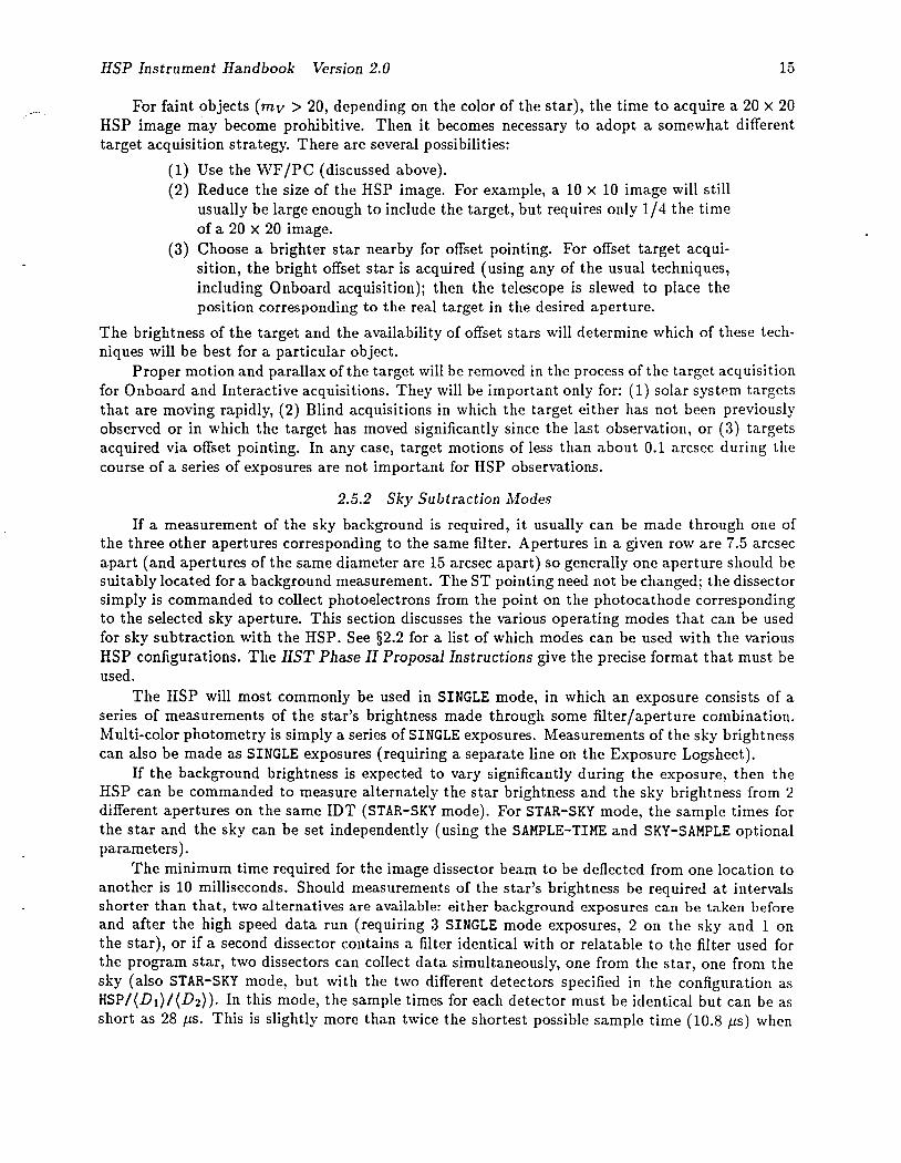
For faint objects (mv > 20, depending on the color of the star), the time to acquire a 20 x 20HSP image may become prohibitive. Then it becomes necessary to adopt a somewhat differenttarget acquisition strategy. There are several possibilities:
(1) Use the WF fPC (discussed above).(2) Reduce the size of the HSP image. For example, a 10 X 10 image will still
usually be large enough to include the target, but requires only 1/4 the timeof a 20 X 20 image.
(3) Choose a brighter star nearby for offset pointing. For offset target acquisition, the bright offset star is acquired (using any of the usual techniques,including Onboard acquisition); then the telescope is slewed to place theposition corresponding to the real target in the desired aperture.
The brightness of the target and the availability of offset stars will determine which of these techniques will be best for a particular object.
Proper motion and parallax of the target will be removed in the process of the target acquisitionfor Onboard and Interactive acquisitions. They will be important only for: (1) solar system targetsthat are moving rapidly, (2) Blind acquisitions in which the target either has not been previouslyobserved or in which the target has moved significantly since the last observation, or (3) targetsacquired via offset pointing. In any case, target motions of less than about 0.1 arcsec during thecourse of a series of exposures are not important for HSP observations.
2.5.2 Sky Subtraction Modes
If a measurement of the sky background is required, it usually can be made through one ofthe three other apertures corresponding to the same filter. Apertures in a given row are 7.5 arcsecapart (and apertures of the same diameter are 15 arcsec apart) so generally one aperture should besuitably located for a background measurement. The ST pointing need not be changed; the dissectorsimply is commanded to collect photoelectrons from the point on the photocathode correspondingto the selected sky aperture. This section discusses the various operating modes that can be usedfor sky subtraction with the HSP. See §2.2 for a list of which modes can be used with the variousHSP configurations. The HST Phase II Proposal Instructions give the precise format that must beused.
The HSP will most commonly be used in SINGLE mode, in which an exposure consists of aseries of measurements of the star's brightness made through some filter/aperture combination.Multi-color photometry is simply a series of SINGLE exposures. Measurements of the sky brightnesscan also be made as SINGLE exposures (requiring a separate line on the Exposure Logsheet).
If the background brightness is expected to vary significantly during the exposure, then theHSP can be commanded to measure alternately the star brightness and the sky brightness from 2different apertures on the same IDT (STAR-SKY mode). For STAR-SKY mode, the sample times forthe star and the sky can be set independently (using the SAMPLE-TIME and SKY-SAMPLE optionalparameters) .
The minimum time required for the image dissector beam to be deflected from one location toanother is 10 milliseconds. Should measurements of the star's brightness be required at intervalsshorter than that, two alternatives are available: either background exposures can be taken beforeand after the high speed data run (requiring 3 SINGLE mode exposures, 2 on the sky and 1 onthe star), or if a second dissector contains a filter identical with or relatable to the filter used forthe program star, two dissectors can collect data simultaneously, one from the star, one from thesky (also STAR-SKY mode, but with the two different detectors specified in the configuration asHSP/(D1)/(D2)). In this mode, the sample times for each detector must be identical but can be asshort as 28 J.LS. This is slightly more than twice the shortest possible sample time (10.8 J.Ls) when
16 HSP Instrument Handbook Version 2.0
only one detector is collecting data. In principle this sample time could be reduced by using aspecial "bus director" program (see §3.1.1).
The SPLIT configuration, in which a beamsplitter sends part of a star's light to two differentdetectors, uses the same technique as two-detector STAR-SKY mode to get simultaneous measurements of a star in two colors. On the other hand, two-color photometry using the PRISM mode isaccomplished using the equivalent of one-detector STAR-SKY mode, switching the beam of a singleIDT between the two apertures associated with a particular prism. Thus, prism mode measurements are not truly simultaneous but are separated by at least 10 milliseconds, just as are allone-detector STAR-SKY measurements.
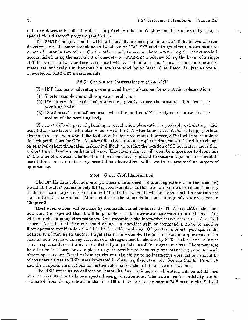
2.5.3 Occultation Observations with the HSP
The HSP has many advantages over ground-based telescopes for occultation observations:
(1) Shorter sample times allow greater resolution.(2) UV observations and smaller apertures greatly reduce the scattered light from the
occulting body.(3) "Stationary" occultations occur when the motion of ST nearly compensates for the
motion of the occulting body.
The most difficult part of planning an occultation observation is probably calculating whichoccultations are favorable for observations with the ST. After launch, the STScI will supply orbitalelements to those who would like ,to do occultation predictions; however, STScI will not be able todo such predictions for GOs. Another difficulty is that atmospheric drag causes the orbit to changeon relatively short timescales, making it difficult to predict the location of ST accurately more thana short time (about a month) in advance. This means that it will often be impossible to determineat the time of proposal whether the ST will be suitably placed to observe a particular candidateoccultation. As a result, many occultation observations will have to be proposed as targets ofopportunity.
2.5.4 Other Useful Information
The 105 Hz data collection rate (in which a data word is 8 bits long rather than the usual 16)would fill the HSP buffers in only 0.16 s. However, data at this rate can be transferred continuouslyto the on-board tape recorder for about 10 minutes, where it will be stored until its contents aretransmitted to the ground. More details on the transmission and storage of data are given inChapter 3.
Most observations will be made by commands stored on-board the ST. About 20% of the time,however, it is expected that it will be possible to make interactive observations in real time. Thiswill be useful in many circumstances. One example is the interactive target acquisition describedabove.' Also, in real time one could change an amplifier gain or command a move to anotherfilter-aperture combination should it be desirable to do so. Of greatest interest, perhaps, is thepossibility of moving to another target star if, for example, the first one was in a quiescent ratherthan an active phase. In any case, all such changes must be checked by STScI beforehand to insurethat no spacecraft constraints are violated by any of the possible program options. There may alsobe other restrictions; for example, it may be possible to have only one branching point for eachobserving sequence. Despite these restrictions, the ability to do interactive observations should beof considerable use to HSP users interested in observing flare stars, etc. See the Call for Proposalsand the Proposal Instructions for further information about interactive observations.
The HSP contains no calibration lamps; its final radiometric calibration will be establishedby observing stars with known spectral energy distributions. The instrument's sensitivity can beestimated from the specification that in 2000 s it be able to measure a 24m star in the B band

HSP Instrument Handbook Version 2.0 17
with a signal-to-noise ratio of 10. Typical image dissector dark counts and currents are less thanD.1/sec and 1 pA, respectively. Chapter 4 gives a detailed description of the IISP sensitivity.
18 HSP Instrument Handbook Version 2.0
Chapter 3: Details of the HSP-ST System
Chapter 2 describes the general characteristics of the HSP in enough detail for most observingprograms. However, sometimes more information will be needed in order to use the IISP as efficiently as possible. This chapter has sections on some internal details of the HSP's operation, onsome quirks and limitations of the HSP-ST system, and on sources of noise in measurements madewith the HSP.
3.1 Internal Details of the HSP
3.1.1 The Bus Director
Individual observing sequences in the HSP are carried out by a "nanoprocessor" called theBus Director (BD). The BD executes a very limited set of 16 instructions which do things like loadthe latches of a particular detector with deflection settings, cause the contents of a counter or anAID converter to be placed into the science data buffer, loop a specified number of times, or waita specified number of clock cycles. (One clock cycle is 1/(1.024 MHz); for convenience this usuallyis referred to as 1 tick.) Thus, a sequence of 100 1 sec samples on a star is executed by a BDprogram that loops 100 times through instructions which start a counter, wait 1 sec, then stop thecounter and put its contents in the science data buffer. All of the different data formats and modesthat are described below are the result of "standard" BD programs; however, it is also possible towrite non-standard programs to produce new modes or formats (e.g., a Star/Sky/Dark sequencewhich measures the dark counting rate separately from the sky background rate, or a data formatin which only the top 2 bytes of the 3 byte digital counter are read out.) It is far beyond the scopeof this manual to give enough information for the reader to write his or her own BD programs;contact STScI for more information if you have an observation that requires a new BD program.
3.1.2 Standard Data Formats
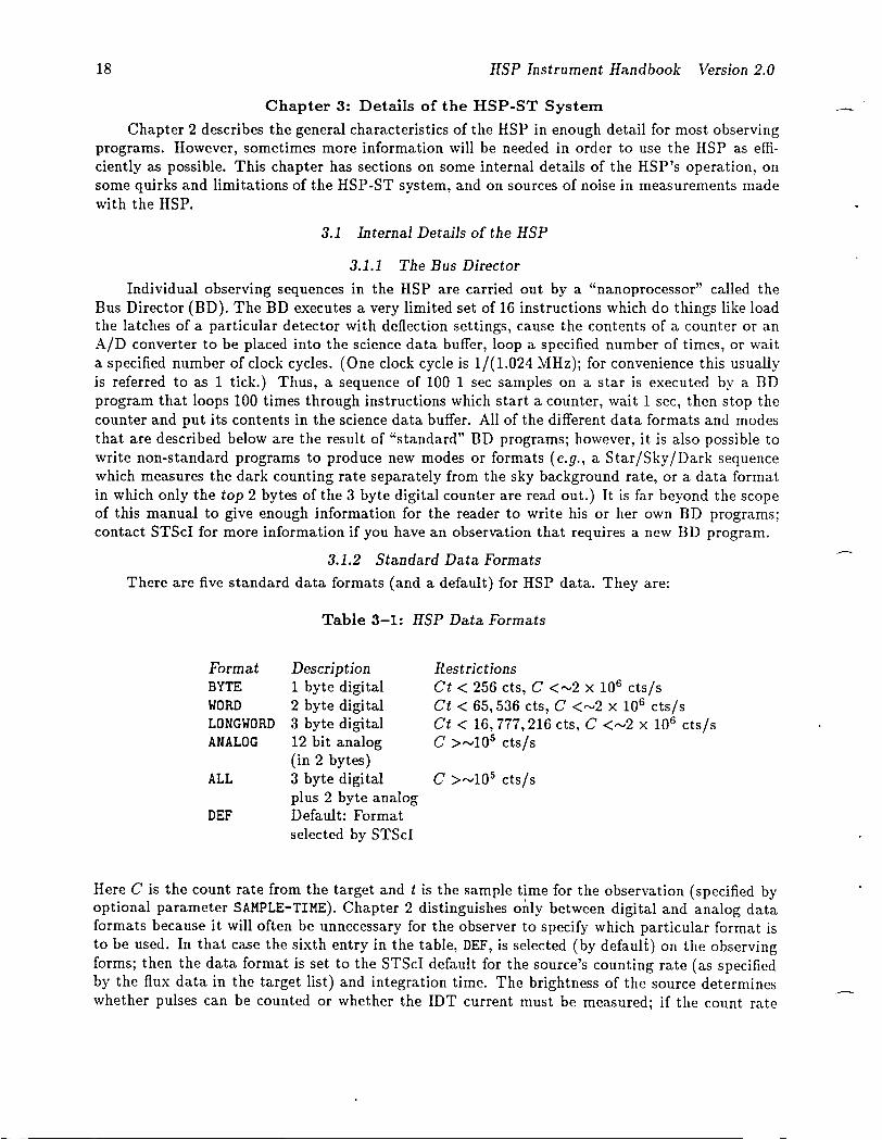
There are five standard data formats (and a default) for HSP data. They are:
Table 3-1: HSP Data Formats
FormatBYTEWORDLONGWORDANALOG
ALL
DEF
Description1 byte digi tal2 byte digi tal3 byte digital12 bit analog(in 2 bytes)3 byte digi talplus 2 byte analogDefault: Formatselected by STScI
RestrictionsCt < 256 cts, C <",2 X 106 cts/sCt < 65,536 cts, C <",2 X 106 cts/sCt < 16,777,216 cts, C <",2 X 106 cts/sC >",105 cts/s
C >"'105 cts/s
Here C is the count rate from the target and t is the sample time for the observation (specified byoptional parameter SAMPLE-TIME). Chapter 2 distinguishes only between digital and analog dataformats because it will often be unnecessary for the observer to specify which particular format isto be used. In that case the sixth entry in the table, DEF, is selected (by default) on the observingforms; then the data format is set to the STScI default for the source's counting rate (as specifiedby the flux data in the target list) and integration time. The brightness of the source determineswhether pulses can be counted or whether the IDT current must be measured; if the count rate
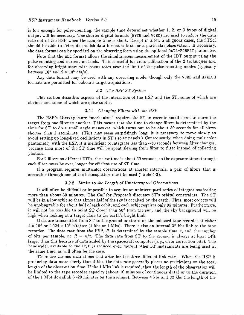
HSP Instrument Handbook Version 2.0 19
is low enough for pulse-counting, the sample time determines whether 1, 2, or 3 bytes of digitaloutput will be necessary. The shorter digital formats (BYTE and WORD) are used to reduce the datarate out of the HSP when the sample time is short. Except in a few ambiguous cases, the STScIshould be able to determine which data format is best for a particular observation. If necessary,the data format can by specified on the observing form using the optional DATA-FORMAT parameter.
Note that the ALL format allows the simultaneous measurement of the IDT output using thepulse-counting and current methods. This is useful for cross-calibration of the 2 techniques andfor observing bright stars with count rates near th~ limit of the pulse-counting modes (typicallybetween 105 and 2 X 10⁶ cts/s).
Any data format may be used with any observing mode, though only the WORD and ANALOGformats are permitted for onboard target acquisitions.
3.2 TIle HSP-ST System
This section describes aspects of the interaction of the HSP and the ST, some of which areobvious and some of which are quite subtle.
3.2.1 Changing Filters with the HSP
The HSP's filter/aperture "mechanism" requires the ST to execute small slews to move thetarget from one filter to another. This means that the time to change filters is determined by thetime for ST to do a small angle maneuver, which turns out to be about 30 seconds for all slewsshorter than 1 arcminute. (This may seem surprisingly long; it is necessary to move slowly toavoid setting up long-lived oscillations in ST's solar panels.) Consequently, when doing multicolorphotometry with the HSP, it is inefficient to integrate less than ",30 seconds between filter changes,because then most of the ST time will be spent slewing from filter to filter instead of collectingphotons.
For 2 filters on different IDTs, the slew time is about 60 seconds, so the exposure times througheach filter must be even longer for efficient use of ST time.
If a program requires multicolor observations at shorter intervals, a pair of filters that isaccessible through one of the beamsplitters must be used (Table 4-3).
3.2.2 Limits to the Length of Uninterrupted Observations
It will often be difficult or impossible to acquire an uninterrupted series of integrations lastingmore than about 30 minutes. The Call for Proposals discusses ST's orbital constraints. The STwill be in a low orbit so that almost half of the sky is occulted by the earth. Thus, most objects willbe unobservable for about half of each orbit, and each orbit requires only 95 minutes. Furthermore,it will not be possible to point ST closer than 50° from the sun, and the sky background will behigh when looking at a target close to the earth's bright limb.
Data are transmitted from ST to the ground or stored on the onboard tape recorder at either4 X 103 or 1.024 X 106 bits/sec (4 kbs or 1 Mbs). There is also an internal 32 kbs link to the taperecorder. The data rate from the HSP, R, is determined by the sample time, t, and the numberof bits per sample, n: R = nit. The data rate from ST to the ground is always at least 14%larger than this because of data added by the spacecraft computer (e.g., error correction bits). Thebandwidth available to the HSP is reduced even more if other ST instruments are being used atthe same time, as will often be the case.
There are various restrictions that arise for the three different link rates. When the HSP isproducing data more slowly than 4 kbs, the data rate generally places no restrictions on the totallength of the observation time. If the 1 Mbs link is required, then the length of the observation willbe limited to the tape recorder capacity (about 10 minutes of continuous data) or to the durationof the 1 Mbs downlink ("'20 minutes on the average). Between 4 kbs and 32 kbs the length of the

20 HSP Instrument Handbook Version 2.0
observation may also be limited: if the tape recorder is not available, the data will have to be sentto the ground at 1 Mbs.
To determine whether these restriction are important for a particular observation, you need toknow the following information:
(1) Is the target in the continuous viewing zone (CVZ)? Targets in the CVZ arecontinuously visible for several days during certain phases of ST's 56-dayorbital precession. Targets not in the CVZ are occulted by the earth onevery orbit.
(2) What is the required data rate? R 2: 1.14n/t, where t is the sample time(determined by your scientific objectives) and n is the number of bits persample (determined from t and from the target count rate C - see Table3-1.)(a) R ~ 4 kbs: no limit on observing time.(b) 4 ~ R ~ 32 kbs: observations may be up to 8 hours long if data are
stored on onboard tape recorder.(c) 32 kbs ~ R ~ 1 Mbs: observations may usually last only 10-20 minutes,
depending on the availability of the 1 Mbs TDRSS link to the ground.
All of these restrictions mean that most observations that require more than 20 or 30 minuteswill probably have gaps in their time coverage. These gaps will obviously lead to some difficultiesin the data analysis (e.g., aliases of the 95 minute orbital period will show up in periodic analyses).Observers should try to anticipate how these problems will affect their projects; if gaps in thedata will make it impossible to achieve the goal of the program, they should be sure to ask forcontinuous observations in the proposal. For some programs it may be necessary to choose targetsin the "continuous viewing zones", small regions near the orbital poles that are visible throughoutthe orbit because they are not occulted by the earth. Note that the continuous viewing zones arealways near the limb of the earth, so sky subtraction may be more critical for such observationsthan for targets far from the limb.
3.2.3 Unequally Spaced Data
Most high speed photometrists are accustomed to using mathematical tools such as fast Fouriertransforms and autocorrelation functions to analyze their data; these tools require that the databe equally spaced. However, another consequence of the ST's low orbit is that data from the HSPoften will not be equally spaced in time. The light travel time from one side of the ST orbit tothe other is about 40 msec. Consequently, observations that have sample times shorter than thisand that last a significant fraction of an orbit will not be equally spaced in the heliocentric restframe. The STSDAS system at STScI will provide software to calculate the time of each samplein the solar rest frame; however, the observer should be prepared to analyze the resulting unevenlyspaced data.
3.2.4 Absolute Timing of Observations
Although the HSP can make observations with sample times as short as 10.8 J-lsec, the absolutetime of an observation can only be established to within a few milliseconds. This happens becausethe phase of the ST onboard clock is only known to a few milliseconds compared to the timeon the ground. The exact accuracy of the clock will be measured after launch; the specificationsrequire the uncertainty to be less than 10 msec, but it is possible that HSP observations of standardsources (e.g., the Crab pulsar) can establish the ST onboard time with greater accuracy. Proposalsthat require absolute timing better than 10 msec should not be submitted until after post-launchcalibration of the clock has been shown to work.
HSP Instrument Handbook Version 2.0 21
3.3 Sources of Noise and Systematic Errors
There are many sources of noise and/or possible systematic errors for the HSP. This sectiondiscusses those that are currently judged to be of possible significance. Which of these are mostimportant will in many cases not be known until after launch.
3.3.1 Noise
"Noise" is here taken to mean random variations in the measured counting rates that wouldaverage to zero in a long series of observations. The noise in most HSP observations will bedetermined by the Poisson statistics for the star, sky, and detector dark counts. The star countingrate obviously depends on the color and magnitude of the star and on the filter used. The skycounting rate has the same dependencies; it also depends on the angle to the sun, the moon, andthe limb of the earth in a complicated and (until launch) unknown way.
Dark counts in the HSP may be produced either by emission of thermal electrons from thephotocathode (f'V 0.1 counts/sec for the IDTs, f'V 200 counts/sec for the PMT) or by impacts ofhigh energy particles on the photocathode and the first dynode. Large particle fluxes like thoseencountered in the South Atlantic Anomaly may also cause the MgFz in the HSP filters andfaceplates to fluoresce for a period of time. The particle background and its effect on the HSPwill vary with the position of the ST in its orbit and will have to be determined from post-launchobservations.
Very bright sources will have to be measured using analog (current) data format because theircounting rates will be too high for the pulse counting electronics. The statistics of noise for thecurrent data format will be determined by the counting rate, the time constant of the currentamplifier, and the sample time. The noise will consequently be somewhat more complicated thansimple Poisson statistics.
Only when the number of photons counted is very large (> 106 ) will other sources of noisebecome noticeable. One such noise source will be the imperfect guiding of the ST pointing system.Guiding errors move the source away from the center of the aperture, decreasing the fraction ofthe source's flux that reaches the HSP detector. Spatial variations in the quantum efficiency ofthe photocathodes may also lead to small variations in the count rate as the image of the starmoves. These fluctuations should be quite small « 0.1%), but will be noticeable if a source isbright enough to be measured to this accuracy in the FGS cycle time of a few seconds.
Fluctuations in the high voltage can change the gain of the photomultiplier sections of theIDTs. This will have little effect on the pulse counting rate, but may change the current out of thetube. The HSP high voltage power supplies have been designed so fluctuations will lead to IDTcurrent variations smaller than 0.1%.
Fluctuations in the low voltages could also affect the performance of the HSP by changing thedeflections and focus of the IDTs, the threshold of the pulse amplitude discriminator, the outputvoltage of the current-to-voltage converter, etc. However, all of these effects have been found to benegligibly small in laboratory testing.
3.3.2 Systematic Errors
The accuracy of the measured brightness will be determined for many sources by systematicerrors which do not average to zero after many measurements. The sizes of systematic errors are
inherently more difficult to determine from observations than are noise amplitudes; this problemis made even harder by the fact that the HSP is capable of making more accurate measurementsthan any ground-based photometer; consequently, the systematic errors of the HSP photometricsystem probably will not be measurable by comparison to observations using other instruments. Itis hoped that the sum of all systematic errors that cannot be removed will be less than 0.1% of thesignal.

22 HSP Instrument Handbook Version 2.0
Small-scale spatial variations in the filters and photocathodes will cause errors in the measuredfluxes since the calibration targets and program targets may not be placed in exactly the samelocations within any given aperture. These errors should not be large because the beam is not infocus at the filters and the photocathodes are quite uniform on small scales. The degree to whichtarget positioning is reproducible depends on the performance of the ST pointing control system,which will not be known until after launch.
Non-linearities in the AID conversion may limi t the accuracy of analog (current) mode measurements. Since the AID converter has 12 bits, even a perfect device cannot measure the currentto an accuracy better than ""0.03%.
Fluctuations from guiding errors, discussed above with reference to noise, can also producesystematic errors. It is likely that the guiding errors will be different for objects with differentguide stars. Consequently, two objects with identical fluxes may have different average countingrates: the one with larger guiding errors will appear to have a smaller flux. It may be possible toremove this effect by analyzing the engineering telemetry from the ST to determine how large theguiding errors were for a particular observation.
The IDTs inside the HSP must warm up for some time before they can be used for accuratephotometry. This warm-up time will be a function of the accuracy that is desired; for example, afew seconds will probably suffice for 10% photometry. The characteristics of the IISP when it iswarming up will not be fully known until after launch.
The changing temperature of the HSP can lead to systematic variations in the counting rate.The photocathode efficiency can vary as a function of temperature; this will be important for thePMT and possibly the bialkali IDTs (VIS and POL), but should not affect the CsTe IDTs (UV1and UV2) which have photocathodes with much larger work functions. All voltages produced byelectronic power supplies will also vary with temperature. Most of these effects will be removed bySTScI through calibration observations at different temperatures.
Chapter 2 mentioned that the flexing of the HSP as its temperature changes causes the imageof the aperture plate to move slightly on the photocathode. If not entirely compensated, thiswill result in the target being improperly centered in the aperture, and its flux relative to thecalibrator (which presumably was centered correctly) will be incorrectly determined. As soon asthe thermal behavior of the HSP-ST system is understood, corrections for the thermal motion ofapertures will be incorporated into the ground system; however, this thermal modeling is expectedto prove difficult. Mis-centering of targets may be the largest single source of systematic error inHSP measurements.
3.3.3 Reducing Systematic Errors
Many of the systematic errors can be reduced greatly by observing a calibration target beforeand after observing program targets. The STScI will eventually determine how often such calibration observations must be done to achieve a given level of accuracy. Note, however, that verycritical observations probably will always require extra calibrations (which will count as part of yourobserving time and which must be requested as separate exposures in your proposal.) Chapter 5describes the standard calibrations that STScI expects to supply for the HSP.
The aperture centering errors can be reduced by using the 1 arcsec diameter apertures ratherthan the 0.4 arcsec apertures. The smaller apertures should be used only when the background isbright compared to the star, when the field is so crowded that the small aperture is necessary toisolate the target, or when the greatest photometric accuracy is not necessary.
Some centering errors may a~so be reduced by "peaking up" before the observation. Peakingup may involve both internal IISP operations-such as a small image to center the IDT beam onthe aperture-and ST operations-such as a dwell scan to center the target in the HSP aperture.The former ought to be fast, while the latter will be slower. There is onboard software to peak-up

HSP Instrument Handbook Version 2.0 23
the IDT read beam on the aperture which can be accessed using the PEAKUP mode; however, theground system does not currently support the use of this software, so observers should confer withthe STScI before using it in their proposals. Using a dwell scan to center the telescope pointing onthe star will require an interactive observation in which the astronomer looks at the data taken atdifferent paintings and identifies which one is the best. This will require a considerable amount oftime, but may be useful for long observations in which it is crucial that the target be well-centered.

24 HSP Instrument Handbook Version 2.0
Chapter 4: Instrument Performance
4.1 Sensitivity of the IISP
This section consists mainly of figures and tables describing the sensitivity of the HSP. Someof the data that are included:
(1) Transmission and/or reflectivity as a function of wavelength for all opticalelements: filters, mirrors, polarizers, and beamsplitters.
(2) Tables giving nominal descriptions of all filters (name, central wavelength,F\VHM, transmission, etc.)
(3) Quantum efficiency as a function of wavelength and dark count rates fordetectors.
(4) Figures giving time to reach SIN 100 for a star of a given magnitude andeffective temperature.
(5) Nominal background counting rates through various filters.(6) The time required for target acquisition as a function of magnitude and color
of the target.
Several explanatory comments apply to all the tables and figures:
(1) Filter names are all of the form Fxxxw where xxx is the central wavelengthof the filter in nm and w is a measure of the width of the filter bandpasswith the following approximate ranges:
N = narrow (FWHM < 5% of central wavelength)M = medium (5% < FWHM < 15%)W = wide (FWHM > 15%)
LP = longpass (filter passes all wavelengths longward of xxx)
(2) "Throughput" means the peak efficiency for the entire HSP/ST system,including reflectivity of mirrors, filter, polarizer, and beamsplitter transmission, and detector efficiency.
(3) "Transmission" means the peak value for the given optical element (filter,polarizer, etc.) alone, not including any other elements in system.
At the end of the chapter is an example that demonstrates how to use the information in thetables and figures to estimate exposure times for HSP observations.

HSP Instrument Handbook Version 2.0 25
Table 4-1: HSP Photometry Filters
Name A FWHM Transmission Throughput Remarks(A) (A) (%) (%)
F122M 1220 130 7 0.05F135W 1350 230 12 0.05F145M 1450 200 13 0.10F152M 1520 180 13 0.13F179M 1790 220 30 0.9F184W 1840 370 31 1.0F218M 2180 170 35 1.3F220W 2200 350 35 1.3F240W 2400 550 48 1.6F248M 2480 370 35 1.2F262M 2620 290 33 1.0 UV2IDT
1.3 VIS IDTF278N 2780 140 33 0.4F284M 2840 380 31 0.8F320Nl 3200 160 26 0.7 PMT beamsplitter (VIS)F355M 3550 310 19 0.6 uF419N 4190 190 31 1.4 vF450W 4500 1400 65 2.9 BF551W 5510 850 38 1.1 VF620W2 6200 1300 1.5 RF750W2 7000-9000 5.4 PMT beamsplitter (PMT)F140LP 1400-3000 90 3.2F160Lp3 1600-3000 90 3.2 UV2 IDT
1600-7000 90 4.2 VIS IDT1600-7000 90 4.6 POL IDT
F400LP 4000-7000 90 3.7
NOTES:(1) Shape ofF320N is determined by band passed by PMT beamsplitter rather than by focal plane
filter. Transmission is for beamsplitter bandpass.(2) Shapes ofR filter (F620W) and PMT filter (F750W) are defined by the photocathode efficiency,
so transmissions for filters alone are not given.(3) F160LP occurs on both CsTe and Bialkali IDTs. The red cutoff is determined by the photo
cathode response in both cases.(4) Unless listed separately, filters that occur on two or three different IDTs have same throughput
on all IDTs.
26 HSP Instrument Handbook Version 2.0
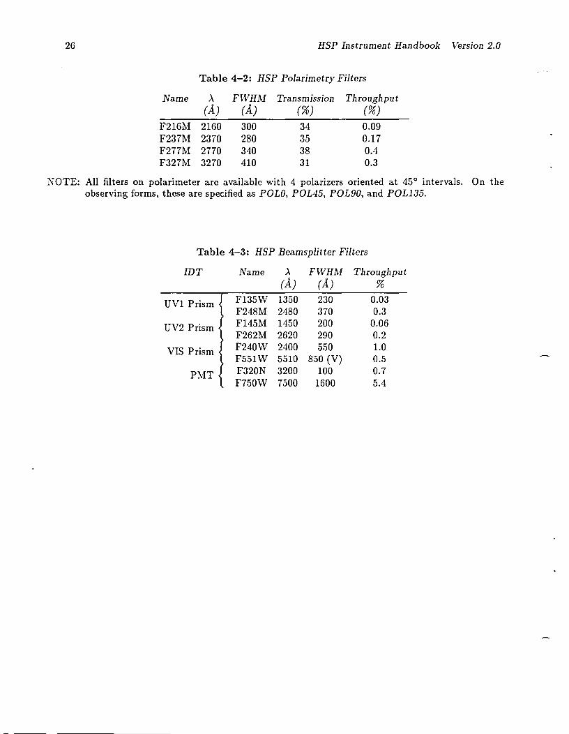
Table 4-2: HSP Polarimetry Filters
Name >. FWHM Transmission Throughput(A) (A) (%) (%)
F216M 2160 300 34 0.09F237M 2370 280 35 0.17F277M 2770 340 38 0.4F327M 3270 410 31 0.3
NOTE: All filters on polarimeter are available with 4 polarizers oriented at 45° intervals. On theobserving forms, these are specified as POLO, POL45, POL90, and POL135.
Table 4-3: HSP Beamsplitter Filters
IDT Name >. FWHM Throughput(A) (A) %
UV1 Prism F135W 1350 230 0.03F248M 2480 370 0.3
UV2 Prism F145M 1450 200 0.06F262M 2620 290 0.2
VIS Prism F240W 2400 550 1.0F551W 5510 850 (V) 0.5
PMT F320N 3200 100 0.7F750W 7500 1600 5.4
HSP Instrument Handbook Version 2.0 27
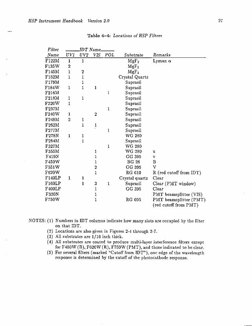
Table 4-4: Locations of HSP Filters
UVlFilterName
__..J.TDT Name, _UV2 VIS POL Substrate Remarks
1
2
1
11
Lyman a
uvBVR (red cutoff from IDT)ClearClear (PMT window)ClearPMT beamsplitter (VIS)PMT beamsplitter (PMT)(red cutoff from PMT)
RG 695
MgF2MgF2
MgF2
Crystal QuartzSuprasilSuprasilSuprasilSuprasilSuprasilSuprasilSuprasilSuprasilSuprasilSuprasilWG 280SuprasilWG 280WG 280GG 395BG 28
GG 395RG 610
Crystal quartzSuprasilGG 395
1
1
1
1
1
3111
11121
11
11 1
2111 1
1
1
12
11
1211
1
F122MF135WF145MF152MF179MF184WF216MF218MF220WF237MF240WF248MF262MF277MF278NF284MF327MF355MF419NF450WF551WF620WF140LPF160LPF400LPF320NF750W
NOTES: (1) Numbers in IDT columns indicate how many slots are occupied by the filteron that IDT.
(2) Locations are also given in Figures 2-4 through 2-7.(3) All substrates are 1/16 inch thick.(4) All substrates are coated to produce multi-layer interference filters except
for F450W (B), F620W (R), F750W (PMT), and those indicated to be clear.(5) For several filters (marked "Cutoff from IDT"), one edge of the wavelength
response is determined by the cutoff of the photocathode response.
28
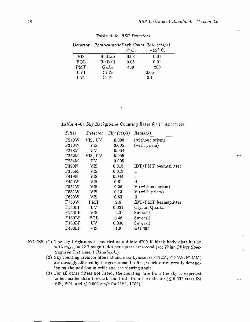
Detector
HSP Instrument Handbook Version 2.0
Table 4-5: HSP Detectors
PhotocatllOdeDark Count Rate (cts/s)00 C. -150 C.
VISPOLPMTUV1UV2
BialkaliBialkaliGaAsCsTeCsTe
0.03 0.010.05 0.01400 200
0.050.1
Table 4-6: Sky Background Counting Rates for I" Apertures
Filter Detector Sky (cts/s) Remarks
F240W VIS, UV 0.008 (without prism)F240W VIS 0.005 (with prism)F248M UV 0.004F262M VIS, UV 0.005F284M UV 0.005F320N VIS 0.015 IDT/PMT beamsplitterF355M VIS 0.019 uF419N VIS 0.044 vF450W VIS 0.61 BF551W VIS 0.26 V (without prism)F551W VIS 0.13 V (with prism)F620W VIS 0.63 RF750W PMT 2.6 IDT/PMT beamsplitterF140LP UV 0.031 Crystal QuartzF160LP VIS 2.3 SuprasilF160LP POL 0.46 SuprasilF160LP UV 0.030 SuprasilF400LP VIS 1.9 GG 395
NOTES: (1) The sky brightness is modeled as a dilute 4700 K black body distributionwith m5556 = 22.7 magnitudes per square arcsecond (see Faint Object Spectrograph Instrument Handbook.)
(2) Sky counting rates for filters at and near Lyman a (F122M, F135W, F145M)are strongly affected by the geocoronal La line, which varies greatly depending on the position in orbit and the viewing angle.
(3) For all other filters not listed, the counting rate from the sky is expectedto be smaller than the dark count rate from the detector (~ 0.002 cts/s forVIS, POL and ~ 0.006 cts/s for UV1, UV2).

HSP Instrument Handbook Version 2.0
Table 4-7: Target Acquisition Time (minutes)
UVl, UV2 IDTs
Effective Temperaturemv 5000 K 10000 K 20000 K 40000 K
15 4 0.4 0.2 0.216 10 0.6 0.3 0.217 25 1.4 0.4 0.318 70 3.5 0.8 0.419 - 8 1.6 0.820 - 20 4 1.821 - 50 10 522 - - 25 1123 - - 70 3024 - - - 75
VIS IDTEffective Temperature
mv 5000 K 10000 K 20000 K 40000 K
15 0.3 0.2 0.2 0.216 0.4 0.3 0.2 0.217 0.6 0.4 0.3 0.318 1.2 0.7 0.4 0.419 3 1.6 0.8 0.620 9 4 2 1.221 30 12 5 322 - 40 15 923 - - 50 2524 - - - -
POLIDT
Effective Temperaturemv 5000 K 10000 K 20000 K 40000 K
15 0.2 0.2 0.2 0.216 0.3 0.3 0.2 0.217 0.6 0.4 0.3 0.318 1.1 0.7 0.4 0.419 3 1.4 0.8 0.520 7 4 1.7 1.121 20 9 4 322 60 25 11 723 - 90 30 2024 - - - 60
NOTES: (1) Time was calculated for a 20 X 20 image with a signal-to-noise ratio of 6 forthe target, including noise from the sky background and dark counts.
(2) An overhead of 25 ms per point is included (10 s for the 20 X 20 image).(3) Times longer than 100 minutes are marked "-".
29

30 HSP Instrument Handbook Version 2.0
HSP Filters: 1000-2500 A
-0.5~o.-~ -1.0.-S~ -1.5
tU~
E- -2.0t:l.Oo~
-2.5
-3·1~00.0
Figure 4-1: HSP Filters: 1000-2500 A
HSP Filters: 2000-3500 A0.0
-0.5~o.-~ -1.0
.......S~ -1.5
tU~
E- -2.0t:l.Oo~
-2.5
2300. 2600. 2900. 3200.
Wavelength (A)Figure 4-2: HSP Filters: 2000-3500 A
3500.
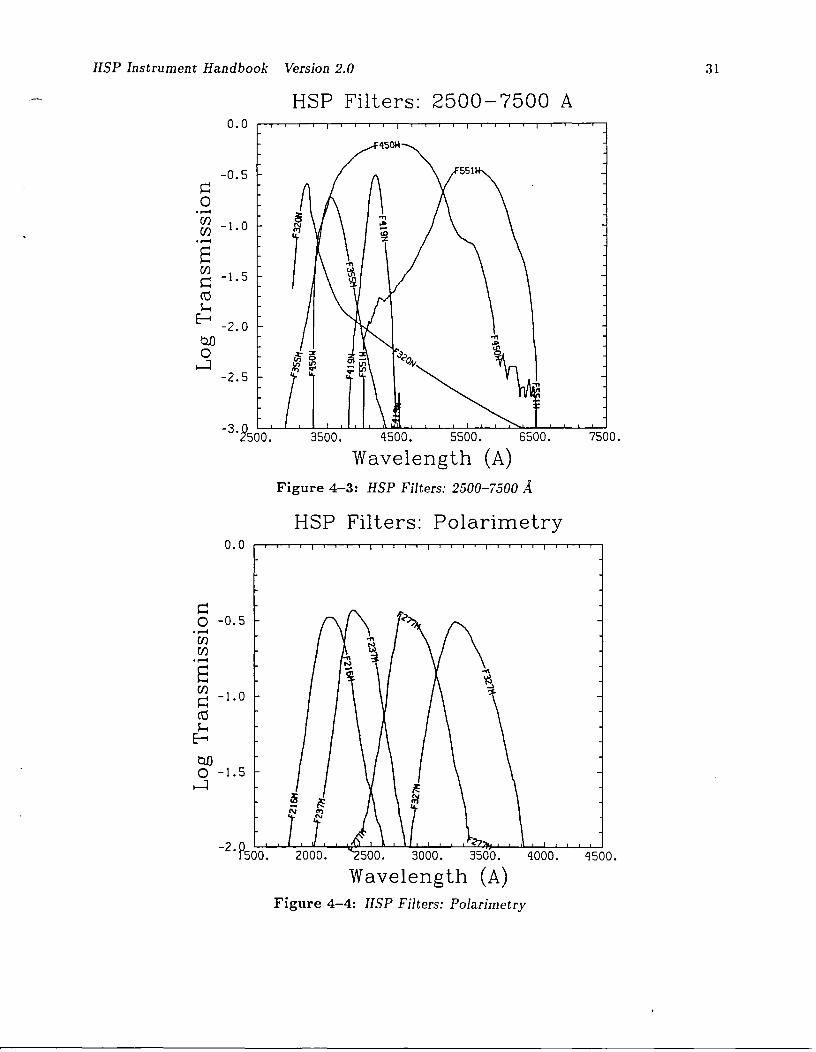
HSP Instrument Handbook Version 2.0
HSP Filters: 2500-7500 A0.0
31
-0.5~o.....~ -1.0.....S~ -1.5
Cds...
E--< -2.0QOo~
-2.5
3500. 4500. 5500. 6500.
Wavelength (A)Figure 4-3: HSP Filters: 2500-7500 A
HSP Filters: Polarimetry
7500.
~o -0.5.....mm.....S~ -1.0
Cds...
E--<QOo -1.5~
- 2•P50'-0........l-L--'-"-'-.............:l""::-~ ..............."'-'-"-'-....l-J~<Jt-I-....l-J .....4'-0"'"-:00:-'-•.....L-J'-4L....J500.
Figure 4-4: IISP Filters: Polarimetry

32 HSP Instrument Handbook Version 2.0
HSP Beamsplitters: Throughput
-4. Pooo.
-1.5
--+-J;j0..-...c: 2.0Q.O~
2 -2.5
...c:~
Q.O-3.0
o~
-3.5F
3000. 5000. 7000.
Wavelength (A)Figure 4-5: HSP Beamsplitter Filters: Throughput
9000.
HSP Long Pass Filters
8000.
.UV'( T
ll.
g...
a..c5..L
fI
~CD,
-0.5
0.0
-2.5
-3·POOO. 2000. 3000. 4000. 5000. 6000. 7000.
Wavelength (A)
co.~
~ -1.0.~
S~ -1.5ro~
~ -2.0Q.Oo~
Figure 4-6: HSP Longpass Filters

HSP Instrument Handbook Version 2.0
HSP Detector Efficiencies33
~C)~ -1.0Q)
.1""""4
C).1""""4t+-t -1. 5t+-t
t:£l
S -2.0::l
-+oJ~ro -2.5::l0'
QD -3.0o~
-3·15000.
...•c:<N
3000. 5000. 7000.
Wavelength (A)9000.
Figure 4-7: HSP Detector Quantum Efficiencies
HSP Prism Characteristics0.0
~o
.1""""4
~ -0.3.1""""4
SlfJ.~ro>-.
b -0.7QDo~
-I. Pooo. 2000. 3000. qOOO. 5000. 6000. 7000.
Wavelength (A)
Figure 4-8: IISP Prism Beamsplitter Characteristics

34 HSP Instrument Handbook Version 2.0
PMT Beamsplitter Characteristics0.0
-0.5~o.-~ -1.0.-S~ -1.5
ttl~
~ -2.0Q1)o~
-2.5
3000. QOOO. 5000. 6000.
Wavelength (A)7000.
Figure 4-9: HSP PMT Beamsplitter Characteristics
HSP Polarizer Characteristics
3000. 3500.
WavelengthQ500.QOOO.
(A)
~ ~\..t\..
o -0.5~.-mrn.-S~ -1.0
ttl~
~
Q1)o -1.5~
Figure 4-10: HSP Polarizer Characteristics
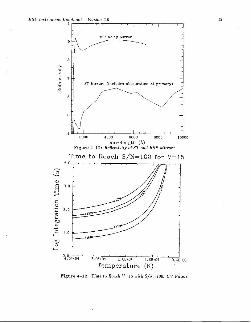
HSP Instrument Handbook Version 2.01.--.---.----,--,-----,-r--.---.----,--,------,-r--.----.-----,--,------,-----,
HSP Relay Mirror.9
35
.8
>.-'.~
-' .7C,)(l)-....(l)
0:::
.6
.5
ST Mirrors (includes obscuration of primary)
I.4 UL...!..---l.----.L--.L----I_.L.-...!..---l.----.L--.L----l_.L.-...l....---l.----.L--.L----l----J2000 4000 6000 8000 10000
Wa·velength (A.)Figure 4-11: Reflectivity of ST and HSP Mirrors
Time to Reach S/N=100 for V=15'1 •0 r-r--r--,....-,r--,-..-..-..--,.~__r__r-,---.-_..,...--,r::__r-r----,---,
..-...rn
"-'"'
Q)
a 3.0• r-i
E-t
~0
• r-i 2.0+Jro~OJ)Q)
+J~ 1.0
>---4
OJ)0~
04.OOE~+-;::O'-:"--'----'----=3~OE:--:0"':-.l.-..l..........::'-=---=-'--'--'--'-...!..--'--'--'-...l....-..J• • + '1 2.0E+0'1 1.OE+0'1 O.OE+OO
Temperature (K)
Figure 4-12: Time to Reach V=15 with S/N=100: UV Filters

O.OE+OO
36 HSP Instrument Handbook Version 2.0
Time to Reach SiN= 100 for V=154.0
...--..rn
"-""
(J)
S 3.0.~
~
~0.~ 2.0~
ro~ f3SSHQ()(J)~ f218H~ 1.0
t--4 f248H
Q()0
.....::1
3.0E+04 2.0E+04 1.0E+04
Temperature (K)Figure 4-13: Time to Reach V=15 with S/N=100: UV, VIS Filters 1
Time to Reach S/N= 100 for V= 153 •0 .........,..........----.---...----.----....-,---,.-----.----.--.---,---,---.-.....-----r--T""r-.........,.........,
...--..rn
"-""2.5
Q)
8.~
~ 2.0
~0.~ 1.5~
ro~ 62OU~Q()
262M-VIS(J) 1.0
~~
~ f7SOWt--4
Q() 0.5 f4SOW
0.....::1
3.0E+04 2.0E+04 1.0E+04
Temperature (K)O.OE+OO
Figure 4-14: Time to Reach V=15 with S/N=100: UV, VIS Filters 2
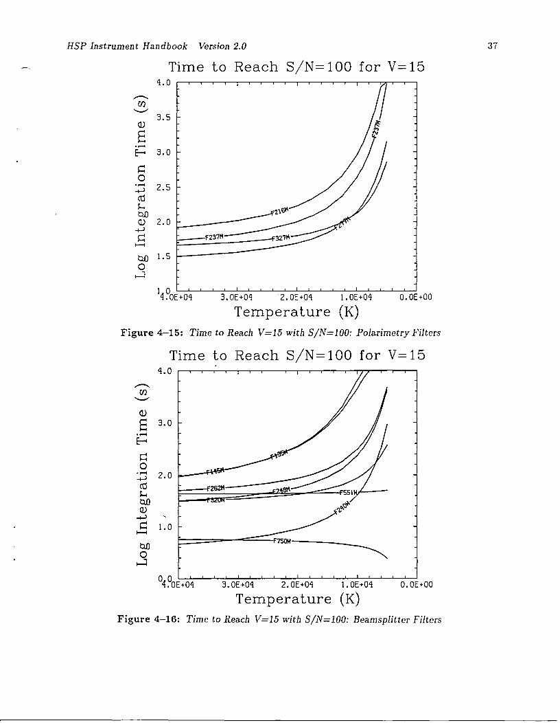
HSP Instrument Handbook Version 2.0
Time to Reach S/N= 100 for V= 154 •0 r--r--'--~~~-'-'---"---"---"T---"T---'----'----r---.----r:;,.,...--.---,
37
---rn'--'"
3.5(])
6......E--< 3.0
~0...... Z.5-+-Jro~
OD(]) Z.O
-+-J~ F237l\
I--i
OD 1.50~
3.0E+04 ·Z.OE+04 1.0E+04
Temperature (K)O.OE+OO
Figure 4-15: Time to Readl V=15 with S/N=lOO: Polarimetry Filters
Time to Reach S/N=100 for V=154•0 r--.--.--~r---;-'-'---"---"T---.---,----,----r---.---rT7t""--.--.--.---,
3.0
Z.O
1.0
3.0E+04 Z.OE+04 1.0E+04
Temperature (K)O.OE+OO
Figure 4-16: Time to Reach V=15 with S/N=100: Beamsplitter Filters

38 IISP Instrument lIandbook Version 2.0
Time to Reach S/N=100 for V=152.5
O.OE+OO1. OE+04
f:- --:;:r-F400LP--
1.5
1.0
2.0
0.5
b.D 0.0o 1-----......:l F\60LP-VlS.PtL
-04:0E+04 3.0E+04 2.0E+04
Temperature (K)Figure 4-17: Time to Reach V=15 with SjN=100: Longpass Filters
4.2 Planning a Typical Observation with the IISP
This section shows how to calculate exposure times, etc., using the information given aboveand in Chapter 3. The example has a relatively simple goal, but it demonstrates some of thecomplications that can arise in planning an observation and shows that the considerations discussedin Chapter 3 are often important.
4.2.1 lIow to Calculate Exposure Times
The exposure time (which must be specified on the exposure logsheet) is the total time STspends pointing at the target from the beginning to the end of the observation. The exact relationbetween the exposure time (texp) and the other times (sample time, delay time, etc.) specified forthe observations depends on the mode used:

HSP Instrument Handbook Version 2.0 39
Configuration
HSP/(D)
HSP/PMT/VISHSP/(D1)/(D2}HSP/(D}
Mode
SINGLE
SPLITSTAR-SKYPRISM,STAR-SKY
Exposure Time
texp = Nsamp(tsamp + tde/av) ,
where N samp is the number of samples desired,t samp is the time for each sample, and tde/av isthe delay time between samples. tde/av is usuallyzero for these modes.t exp = Nsamp(tsamp + tde/av)
t exp = Nsamp(tsamp + tde/av)
t exp = Nsamp(tsamp,tot + tde/av,tot) ,
where tsamp,tot is the sum of the sample timesfor the two apertures and tde/av,tot is the sum ofthe delay times for the two apertures. tde/ay isusually 10 milliseconds for each aperture in thesemodes, so tde/ay,tot is usually 20 milliseconds.
If a sequence containing a number of exposures is defined, then the total exposure time for thesequence is simply the sum of the individual exposure times.
The sample time and number of samples needed for a particular observation are determinedby the scientific objectives of the program: the brightness of the target, the filter used, the timeresolution needed, the signal-to-noise required, etc. The next section shows how to calculate thesample time and number of samples for a typical HSP observation.
4.2.2 Polarimetry of the Crab Pulsar
The Crab pulsar is a classic object for high speed photometry. The scientific goal of this sampleprogram is to measure the polarization of the ultraviolet pulse from the Crab pulsar. We want tohave about 30 bins across the pulse and to collect about 104 photons per bin at the peak of thepulse in order to measure the brightness of the pulse to about 1% and the polarization to ",1.5%.
The (time-averaged) de-reddened spectrum of the Crab pulsar in the UV is approximately
. -29 ( V ) -0.5Fv = 5 X 10 lOIS Hz Wm-2Hz-I
or
(A) -1.5
F)" = 1.5 X 10⁻¹⁴ -'-- erg cm-2 s-I A-I3000A
(e.g., see Pulsars by Manchester and Taylor). The extinction to the Crab pulsar is A v = 1.6m; fromthe standard interstellar reddening curve (tabulated in the Faint Object Spectrograph InstrumentHandbook)' we can calculate the reddened flux at the wavelengths of the filters we are going touse. Then the counting rate in each filter can be estimated from the data for the polarimetry filtersgiven in Table 4-2:
Filter A A)" F)" FWHM Tllroughput Count Rate(A) (mag) (photons cm-2s-1 A-I) (A) (%) (cts/s)
F237M 2370 4.12 6 X 10⁻⁵ 280 0.17 1.2F277M 2770 3.07 1.4 X 10⁻⁴ 340 0.39 8F327M 3270 2.57 2.0 X 10⁻⁴ 410 0.29 11
The counting rate is the product of the photon flux density, the collecting area of ST (rr[120 emF),the FWHM of the filter, and the throughput of the system.

40 HSP Instrument Handbook Version 2.0
To calculate the exposure time; several other factors must be taken into account. The amplitude of the pulses is such that the peak brightness of the pulsar is about 10 times the averagebrightness. Thus, the total exposure time required to get 104 counts at the peak brightness rangesfrom 1.5 minutes to 15 minutes. If the pulse period gets divided into 30 bins (each of about 1 msecduration), then the total observing time must be 30 times that required for the peak bin; it rangesfrom 45 minutes to 7 hours for the filters listed. Finally, it is necessary to make successive observations through each of the four polaroids associated with each filter, increasing the time requiredby another factor of 4. Thus we arrive at the following exposure times:
Filter Observation Time(hours)
F237MF277MF327M
2843
Apparently the pulsar is too faint (mainly because the interstellar extinction is so large) toallow an accurate measurement of the polarization at 2370 A in a reasonable length of time.Consequently, the 2770 A filter is the best choice for the observation.
The sky brightness is relatively small compared to the brightness of the Crab pulsar, so wewill not bother to measure or subtract the sky background. This means that we will use SINGLEmode. Only 1 arcsec apertures are available for polarimetry, but they would be preferred for highaccuracy even if the 0.4 arcsec apertures were available.
The sample time should be somewhat shorter than a millisecond to make the rebinning of thedata into 1 msec bins easier (see §3.2.3); 0.5 msec is a good choice because then the data rate willbe about 16 kilobits per sec, which is comfortably under the 32 kbs rate at which the tape recorderstores data (see §3.2.2). (There is no way to get the data rate under 4 kbs.) There will inevitablybe gaps in the time coverage due to occultations by the earth (§3.2.2), but the period of the Crabpulsar is so well known that the gaps should not pose any data analysis problems. If there areunexpected problems, the pulsar is bright enough to determine the phase of a short segment ofdata from the data itself.
To minimize the systematic errors resulting from mis-centering the pulsar within the apertures,we might want to peak up before beginning the observation (see §3.3.3). However, peaking up willprobably not be necessary in this case because the polarimetry IDT does not suffer from thermalmotion of the aperture images (as do the other IDTs), so its aperture positions will be known verywell.
To minimize other systematic errors, the data taken through differently oriented polaroidsshould be interleaved rather than being taken all at once. Moving from one aperture to the next(by slewing the telescope) requires about 30 sec (§3.2.1); thus, changing polaroids every 10 minuteswill increase the total observing time by only about 10 minutes (20 extra slews at 30 seconds perslew).
Finally, it is necessary to specify how the target will be acquired. It should be possible touse the Onboard target acquisition method, in which an HSP image is automatically analyzed toidentify and locate the target (§2.5.1). The Crab pulsar is bright enough that it is easily detectedin the minimum target acquisition time of 0.2 minute (Table 4-7). However, it is prudent to specifyexplicitly that the integration time at each point in the image is to be 90 msec; then we can besure that the rapid pulses will not cause problems. Remember that the points in an HSP image areaccumulated one at a time, so a target that varies during the target acquisition data collection maybe misidentified or missed entirely. The total target acquisition time for the Crab Pulsar (includingthe 25 ms per point overhead) is then 400 X (25 +90) ms = 46 s (Table 4-7). Since we are observingwith the polarimetry IDT, we will use the target acquisition aperture on the POL IDT.

HSP Instrument Handbook Version 2.0 41
Chapter 5: Standard Calibrations and Data Products
This chapter describes the way HSP data are usually calibrated and what data products result.
5.1 "Pipeline" Calibrations
The raw data received from the ST pass through an automatic calibration procedure calledthe "pipeline" before it is received by the observer. For the HSP the pipeline performs 6 steps:
(1) Reformatting. The data are put in a standard form which is independent of theparticular way it was collected. Interleaved data taken in STAR-SKY mode are dividedinto two files; data taken with the ALL data format is split into separate digital andanalog files. Each data sample (which may be from 8 bits to 24 bits long) is convertedto a 32-bit floating point number. The data is written to a FITS-like format called"GElS" format which can be read directly by the STSDAS analysis routines.
(2) Convert counts to count rates and apply deadtime correction. For pulse-counting(digital) data, the raw counts are divided by the sample time to yield count rates,which are then corrected for the non-linearities caused by the deadtime ofthe countingelectronics. This correction is 1% for counting rates of about 2.5 X 10⁵ counts/soThe deadtime is known from laboratory measurements to be a weak function oftemperature, so it should be possible to make accurate dead time corrections for countrates up to at least 106 counts/so
(3) Subtract dark counts or currents. The standard dark contribution from the phototubeis subtracted. Nominal dark counts and currents are known as a function of both theposition on the IDT cathode and the detector temperature. Notice that if a specialdark calibration is requested by the observer (via the DARK internal calibration targetrequest described in the Phase II Proposal Instructions), it will not be subtractedin the pipeline; instead, it will have to be subtracted using the general purpose dataanalysis system, STSDAS (see below).
(4) Convert currents to equivalent count rates. For current (analog) data, the photocurrents that were measured are converted to the effective count rates that would havebeen measured by a pulse-counting system with zero deadtime.
(5) Correct for the instrumental efficiency. The instrumental efficiency is measured byobserving a standard star through the same aperture-filter combination. Comparisonof observations of the same standard star taken at different times allows the removal ofchanges in the HSP sensitivity as a function of time. The pipeline calibration programcomputes the HSP count rate the target would have had if the HSP sensitivity hadnot changed.
(6) Divide observations of extended objects by aperture area. Note that this applies tosky observations as well as to observations of extended targets.
5.2 Data Products
The results of the pipeline calibration are files containing the HSP count rates as a functionof time for the star+sky and (if it was measured) the sky. In addition, the reformatted data(produced by step 1 above) are readily available to the observer. A single observation can generateup to 8 separate data files: a STAR-SKY observation using the ALL data format will generate anuncalibrated data file and a calibrated data file for each of the star/digital, star/analog, sky/digital,and sky/analog data.
Note that the sky background is not subtracted from the star+sky measurement. It wasdecided that sky subtraction is sufficiently complicated that it is not reasonable to include itin the automated pipeline. Instead, it will be the observer's responsibility to decide how the
42 HSP Instrument Handbook Version 2.0
sky measurements are to be averaged and interpolated before they are subtracted from the starmeasurements.
Note also that the HSP count rates are not translated either to absolute fluxes or to a standardmagnitude system. Both of these conversions depend on knowing the spectral energy distributionof the target star. Keywords in the header of the data will allow conversion to fluxes; the ScienceData Analysis System (STSDAS) at STScI will include the tools that are necessary to convert HSPcount rates to a standard magnitude system if the target star's color is known or if some shape forthe spectrum is assumed. STSDAS will also have access to the calibration data that are requiredfor these translations (e.g., color terms for standard filters and the absolute flux distribution forcalibration stars.)
An advantage of supplying the data in the form of HSP count rates rather than absolute fluxesis that the former are independent of the flux distribution assumed for the standard stars. Thus,if the flux scale of the standard spectra is revised, the HSP count rates will not change.
5.3 Special Calibrations
Calibration observations made as a service by the STScI will be sufficient to calibrate most IISPobservations. However, there will inevitably be some observations that require special calibrations.For example, a special calibration may be required to measure the strongly varying sky backgroundwhich is seen during a lunar occultation. As another exampie, it may be desirable to observe astandard star before and after the target is observed in order to remove small systematic effects(see chapter 3 for more discussion of this).
Any special calibration observations must be requested as part of the observing proposal. Theobserver is responsible for applying the calibration to the data. It is impossible to say at thistime what the accuracy of the standard calibrations will be during the first year after launch, butultimately the goal will be to remove all systematic effects larger than 0.1% of the signal. Smallereffects will probably always be the responsibility of the observer, and larger effects will almostcertainly be present during the year following launch.
HSP Instrument Handbook Version 2.0
Chapter 6: Bibliography
43
White, R. L. 1989, HSP Target Acquisition Handbook. [Description of the various target acquisitionstrategies using the HSP.}
Bless, R. C. 1982, "The High Speed Photometer for the Space Telescope", in The Space TelescopeObservatory, ed. D. Hall, NASA. [A general overview of the HSP, from which much of Chapter2 was taken.} .
White, R. L. 1983, Effect of Guiding Errors on Scientific Performance of ST Instruments, STScIInstrument Science Report GEN-OOl. [Describes how pointing jitter affects the science datafor all the ST instruments.}
Phillips, W. 1984, System Controller User's Manual, University of Wisconsin. [Describes tIle internal electronics of the HSP in gory detail, including a section on how to program the BusDirector.}
White, R. L. 1984, Timing Considerations for HSP Data Collection, STScI Instrument ScienceReport HSP-OOl. [Technical description of the contraints on collecting continuous data withthe HSP.]
1990, Call for HST Observing Proposals, Space Telescope Science Institute. [General informationabout the ST observatory.}
1990, Hubble Space Telescope Phase II Proposal Instructions, Space Telescope Science Institute.[Detailed information about how to fill out the exposure logsheets, target lists, etc., properly.}
Ford, H. C. 1985, Faint Object Spectrograph Instrument Handbook, Space Telescope Science Institute. [Includes some information that may be useful for estimating the signal-to-noise forHSP observations, e.g., references for spectral energy distributions and tables of interstellarreddening.}