1998 fellows thesis h3612
TRANSCRIPT

CHARA CTERIZA TION AND CPDM MODELING OF VOLATILE FATTY
ACID FERMENTATION PVTH COTTON GIN TRASH AND CHICKEN
MANR URE AS SU8STRA TES
A Senior Thesis
By
Joseph Han
1997-98 University Undergraduate Research Fellow
Texas ARM University
Group: Engineering I

Characterization and CPDM Modeling of Volatile Fatty Acid
Fermentation with Cotton Gin Trash and Chicken Manure as
Substrates
by
Joseph H. Han
Submitted to the
Office of Honors Programs and Academic Scholarships, Texas A&M University
in partial fulfillment of the requirements for
1997-98 UNIVERSITY UNDERGRADUATE RESEARCH FELLOWS PROGRAM
Approved as to style and content by:
Mark T. Department
isoi'
ical Engineering
Susanna Finnell, Executive Director Honors Programs and Academic Scholarships
April 16, 1998 Fellows Group: Engineering I

Acknowledgments
I would like to express my thanks to Dr. Mark Holtzapple for giving me to
opportunity to work on his research team. A "leap of faith" is often necessary to trust an
undergraduate to do quality research. I would also like to thank Kyle Ross, Susan
Burdick, and Vincent Chang who helped me with the immense learning curve in the
laboratory. I would like to express my gratitude to the student workers without whom
much of the work would never get done.
I would also like to express my appreciation to Dr. Edward Funkhouser and the
University Honors Program staff. Without the efforts of Dr. Funkhouser and the staff,
many undergraduates would miss the opportunity to experience research.
I would also like to thank Mr. Randy Marek for his help when something needed
to be built or fixed.

Table of Contents
Acknowledgments.
Table of Contents . .
List of Figures. . Vl
List of Tables . vn
Absn. act
Introduction . .
Factors Affecting Product Yields.
Reactors . .
Residence Time.
pH of the Solution.
Methanogenesis.
Oxygen Contamination
Substrate selection/ratio. 10
Temperature . . . . .
Modeling Using the CPDM Method.
Experiments . . . 13
Diffusion of Oxygen Through Reactor Walls . . . . . 13
Batch Municipal Solid Waste/Sewage Sludge. 13
Municipal Solid Waste / Sewage Sludge, Batch Reactor A . . . .
Municipal Solid Waste / Sewage Sludge, Batch Reactor B. . . . .
. . . 13
. . . . I 5
Batch Cotton Gin Trash / Chicken Manure 15
Cotton Gin Trash / Chicken Manure, Batch Reactor 90 g solids/L . . . . . . 16
Cotton Gin Trash / Chicken Manure, Batch Reactor 200 g solids/L . . .
Cotton Gin Trash / Chicken Manure, Batch Reactor 300 g solids/L . . .
. . . 1 7
. . . 1 8
Cotton Gin Trash / Chicken Manure, Batch Reactor 350 g solids/L . . . . . . 19
CPDM Modeling using GT / CM Batch Data. .
CPDM Modeling Using Initial Data Points.
20
20
CPDM Modeling Using All Data Points . 24
Countercurrent Cotton Gin Trash/Chicken Manure. 25
Results and Conclusions 27
Literature Cited . 29
Appendix.
A. Full Data Sets.
Municipal Solid Waste / Sewage Sludge, Batch Reactor A . . .
30
30
. . . . 30
Cotton Gin Trash / Chicken Manure, 90 g solids/L 30
Cotton Gin Trash / Chicken Manure, 200 g solids/L . . . . . 31
Cotton Gin Trash / Chicken Manure, 300 g solids/L. 31
Cotton Gin Trash / Chicken Manure, 350 g solids/L. . . . . 31
Cotton Gin Trash / Chicken Manure, Countercurrent.
B. CPDM Modeling with Initial Data Points .
32
33
Specific Rate Parameter Determination. 33
Batch Reactor Simulation. 34
C. CPDM Modeling with All Data Points . . . 37
Specific Rate Parameter Determination. 37
Batch Reactor Simulation. 38

D. Apparatus and Procedures. . . . . . . 41
Reactors. . . 41
Rolling Mechanism, . 41
Head Gas Measurement . . . 42
Countercurrent Procedures, . . 43
Liquid Product Characterization . . . 44
E. Equipment Parts.
R Supplier Information. .
. 46
. 47

List of Figures
Figure 1. Schematic of the MixAlco Process.
Figure 2. Pathway for Rumen Digestion.
Figure 3. Batch Reactor .
Figure 4. Fed-batch Configuration . .
Figure 5. Countercurrent Configuration. .
Figure 6. MSW / SS Acid Concentration, Batch Reactor A.
Figure 7. MSW / SS Acid Concentration, Batch Reactor B . . . . . . . . 1 5
Figure 8. GT / CM Acid Concentration, 90 g solids/L . . 16
Figure 9. GT / CM Acid Concentration, 200 g solids/L .
Figure 10. GT / CM Acid Concentration, 300 g solids/L
Figure 11. GT / CM Acid Concentration, 350 g solids/L
. . 17
. . 18
19
Figure 12. Polynomial Fit, Batch Reactor 90 g solids/L. . . . . . 20
Figure 13. Polynomial Fit, Batch Reactor 200 g solids/L.
Figure 14. Polynomial Fit, Batch Reactor 300 g solids/L.
Figure 15. Polynomial Fit, Batch Reactor 350 g solids/L.
21
21
. 22
Figure 16. Predicted Acid Concentration, 90 g solids/L. . 23
Figure 17. Predicted Acid Concentration, 200 g solids/L.
Figure 18. Predicted Acid Concentration, 300 g solids/L
. 23
. 24
Figure 19. Predicted Acid Concentration, 350 g solids/L
Figure 20. GT / CM Acid Concentration, Countercurrent.
. 24
. 26

vn
List of Tables
Table l. Annual U. S. Waste Biomass Collected .
Table 2. Substrate Combinations. . . 10
Table 3. MSW / SS Acid Concentration, Batch Reactor A
Table 4. MSW / SS Acid Concentration, Batch Reactor B.
. . 14
. . 15
Table 5. GT / CM Acid Concentration, 90 g solids/L. . . . . . . 16
Table 6. GT / CM Acid Concentration, 200 g solids/L. . . , . . . 17
Table 7. GT / CM Acid Concentration, 300 g solids/L . . 18
Table 8. GT / CM Acid Concentration, 350 g solids/L. . . . . . . 19
Table 9. Specific Rate Parameters, Initial Data Points.
Table 10. GT / CM Acid Concentration, Countercurrent.
22
. . . 25

Abstract
With literally tons of biomass produced annually, a process that uses this waste as
a feedstock would help reduce the problem of disposal. The MixAlco process is one that
does just that. It converts biomass through anaerobic fermentation into volatile fatty
acids, mixed alcohols, and ketones. These products can be used as raw chemicals or as
fuel for their heating value. The process must be implemented on an industrial scale in
order to obtain significant amounts of the products.
The substrates evaluated in this study are municipal solid waste (MSW), sewage
sludge (SS), cotton gin trash (GT), and chicken manure (CM). The product
concentrations obtained from using MSW and SS as the substrate were low compared to
those obtained with GT and CM. Maximum product concentrations when using GT and
CM at a temperature of 55'C were 22 g of total acid/L with acetic acid constituting 78 '10
of the total acids.
The Continuum Particle Distribution Modeling (CPDM) method is iso applied to
data collected for batch reactions. The model can accurately predict acid concentrations
when excessive decomposition of the acid is not occurring. However, when liquid
residence times are extended and the products decompose, the model does not accurately
predict the decreasing product concento'ations.

Introduction
Environmental concerns have increased dramatically in the past years. One
concern is the amount of waste generated per year and how to dispose of the waste.
Literally tons of waste biomass is produced annually. For example, data shown in
Table 1 are estimates for annual biomass waste collected in the United States.
Table 1. Annual U. S. Waste Biomass Collected
Biomass Source Dry Tons/Year (millions)
Manure 174
Municipal Solid Waste 170
Crop Residues 64
Raw Sewage 60
(Chermisino ff et al. , 1980)
The MixAlco process is a fermentation process that uses biomass waste as a raw material.
Anaerobic fermentation processes have been utilized for over a century (McCarty,
1982). Originally, the fermentation process treated municipal wastewater and the
suspended organic material. The purpose of the anaerobic treatment was to aid in the
disposal of the solid sludge. The process decomposed the material to carbon dioxide and
methane. Even in 1895, the value of the decomposition products was recognized
(McCarty, 1982). Donald Cameron of Exeter, England utilized the methane from the
process for heating and lighting at the treating facility.

The MixAlco process is different from earlier processes in that value is placed on
products other than methane. A schematic of the MixAlco process is shown in Figure l.
Biomass Water Mixed
Acid
Salts
Mixed
Organic
Acids
Lime
Kiln
Calcium Carbonate
Fermentation Recovery Treatment
Conversion
Pyrolysis
Hydro genator
Mixed
Ketones
Mixed
Alcohols
(Loescher, 1996)
Figure 1. Schematic of the MixAlco Process
The MixAlco process is modeled after the fermentation that occurs within ruminant
animals. Volatile fatty acids (VFA) are the products of microbial digestion in the rumen
(France and Siddons, 1993). The fermentation produces principally acetic, propionic, and
butyric acids. Higher acids are also produced in lesser amounts. These products can then
be converted to their respective alcohol or ketone. The acid can be used in other
processes, and the alcohol and ketone forms can be used for heating and fuel uses.
Today, these products have a higher market value than methane.
Early studies placed biomass in the rumen of a fistulated steer, Because of
evolution and natural selection, the microorganisms within the rumen are well suited to
digest dietary carbohydrates. These carbohydrates consist of cellulose, hemicellulose,
pectin, starch, and soluble sugars (France and Siddons, 1993). These substrates are first

degraded into their constituent sugars and then fermented to VFA. A representation of
the pathway for the carbohydrates is shown in Figure 2.
Cellulose Starch Soluble sugars
Pentoses
Hemicellulose
Hexoses
Embden-Meyerhoff pathway
Pentose cycle
Pyruvate
Formate
Acetyl CoA
CO2™g
Acrylate ~ pathway
Succin ate pathway
Methane Acetate Buty rate Propionate
(France and Siddons, 1993)
Figure 2. Pathway for Rumen Digestion
Methanogenic bacteria in stagnant ponds and compost piles employ similar pathways
(McCarthy, 1982).
The purpose of this study is to improve acid production &om the MixAlco
process. This process, once implemented on an industrial scale, could be used as a
supplement to current energy sources. In order for the process to be economical, a
minimum of 20 g of acid/L must be produced.
The production of acid depends on several variables. Reactor configuration,
residence time, pH of the solution, methanogenesis, oxygen contamination, substrate

choice, and temperanire all play roles in determining the acid concentration. It is difficult
to determine exactly what role each factor plays; therefore, an empirical method will be
used to model the system. The Continuum Particle Distribution Modeling (CPDM)
method developed by Loescher (1996) will be used. Originally, the method was
developed using mixed winter grass as the substrate. This study will extend the
application of the modeling method to cotton gin trash and chicken manure.
Factors Affecting Product Yields
Reactors
The reactors are an integral component of the MixAlco process. Not only are they
the place where the decomposition occurs, but the reactor configuration is a variable in
determining residence time for the liquids and solids. Three possible types of reactors are
batch, fed-bath, and countercurrent,
The batch configuration employs one reactor. The reactor is initially loaded with
the substrate and media and inoculated with the bacteria. At the conclusion of the
digestion, the product solids and product liquids are removed and characterized, This
configuration is shown in Figure 3.

Substrat
Medi Reactor Reactor
Product Solid~
Product Liquidly
Bacteri
Initial Time Final Time
Figure 3. Batch Reactor
Samples may be removed periodically from the system to determine the extent of the
reaction.
The fed-batch configuration also employs only one reactor. Similar to the batch
configuration, the reactor is initially loaded with the substrate, media, and bacteria.
However, at a future time, the product solids and product liquids are removed, and new
substrate is added. Also fresh media is added; however, the fermentation microorganisms
are allowed to reproduce naturally and sustain their population. This configuration is
shown in Figure 4.
Substrat
Media Reactor
Subsirat
Media Reactor
Product Solid~
Product Liquidly
Bacteri
Initial Time Final Time
Figure 4. Fed-batch Configuration
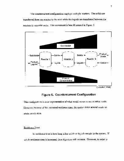
The countercurrent configuration employs multiple reactors. The solids are
transferred from one reactor to the next while the liquids are transferred between the
reactors in opposite order. This movement is best illustrated in Figure 5.
Conversion
— Substrat
Product Liquids
Reactor 1
Solid
Liquid
Reactor 2
Solid
Liquid
Reactor 3
Product Solids
Media—
Product Concentraton
(Loescher, 1996)
Figure 5. Countercurrent Configuration
This configuration is most representative of what would occur on an industrial scale.
However, because of the increased residence time, the system takes several weeks to
attain steady state.
Residence Time
The residence time is how long either solids or liquids remain in the system. If
solids residence time is increased, then digestion will increase. However, in order to

accommodate the increased solid residence time, larger reactor capacity must be
available. The increased digestion improves yields and efficiency of the process;
however, increased costs are associated with the larger reactor.
Liquid residence time determines the final concentration of acids in the product
liquid. By decreasing liquid residence time, the media is circulated through the system at
a faster rate, and product acids do not accumulate in the media. The increased rate
requires a greater amount of fresh media to be introduced into the system and makes it
more difficult to recover the volatile fatty acids from the product liquid because of the
low final concentration. Again, a trade-off exists between improved production and
costs.
gH fth Slti
The pH of the media affects production in two ways. Lower pH's indicate the
presence of acids produced &om the biomass degradation. With the presence of the
acids, the bacteria may be inhibited from further digesting the biomass.
However, a low pH aids production by limiting methanogenesis (Zehnder et al. ,
1982). In the degradation of biomass, methane is produced by the reduction of VFA's.
By preventing this final step, more of the products from the reaction are kept in the VFA
form rather than methane and carbon dioxide.
These issues are acknowledged in this study by the use of two additional
chemicals. Calcium carbonate, CaCOs, is added to the system to convert the product
acids to their respective salt forms. This conversion prevents inhibition. Urea, CH4NiO,

is added to control the pH of the solution and to provide a nitrogen source for protein
synthesis.
M~th
As stated earlier, methane is an undesired product from the biological digestion
pathway. To control the production of methane, iodo form, CHI&, is added to the system.
Because of the similar structure to methane, iodoform is thought to occupy the active sites
where methane is produced. By limiting this production, products of the decomposition
are kept in a more desirable form.
To make the addition of iodoform easier, a solution of 2'/0 by weight in ethanol is
used. The target concentrations of iodoform in solution when added to the reactor is
5 ppm. For batch reactors, the iodoform is added once when the reaction is started. For
fed-batch and countercurrent reactors, iodoform is added to each reactor whenever new
substrate is added or products are transferred.
Ox en Contamination
Because the MixAlco process is based on anaerobic fermentation, oxygen would
limit production of VFA's. The contamination of oxygen is limited during handling by
using nitrogen gas to purge the reactors during product transfer. Also, once the transfer is
complete, a nitrogen blanket is placed in the reactor.

10
Additionally, the liquid media contains an oxygen scavenger. Cysteine sulfide is
added to the media before use to trap any oxygen molecules that may diffuse into the
media.
Substrate selection/ratio
Feedstock to the MixAlco process is usually a combination of two substrates.
One substrate is chosen for its carbohydrate content, and a complement is added as
nutrients for the bacteria. Two such combinations are shown in the table below.
Table 2. Substrate Combinations
Combination Cellulose Source Nutrient Source
¹1 Municipal Solid Waste (MSW) Sewage Sludge (SS)
¹2 Cotton Gin Trash (GT) Chicken Manure (CM)
These substrates can contain an extensive lignin network that limits enzymatic access the
carbohydrates. By pretreating the substrate with lime, Ca(OH)t, many beneficial results
are obtained (Chang). Most notably, an increase of both available sites and surface area
for enzymatic degradation increases acid production.
The ratio of the two substrates in each combination can affect the acid production
rate. A ratio between 80:20 to 60:40 for cellulose source to nutrient source is used
(Rapier, 1995).

~Tt Temperature affects the rate at which bacteria digests the subsnate. Several
temperature ranges exist. Mesophilic is usually defined as ranging from 35'C to 45'C.
Thermophilic temperatures are usually 55'C to 65'C. A higher temperature increases the
production rate; however, the higher temperature also increases the rate at which the
product acids are reduced to carbon dioxide. The experiments in this study were
conducted at a temperature of 55'C.
Modeling Using the CPDM Method
The kinetics of a reaction describe the rate at which the reaction occurs. For the
MixAlco process, the kinetics would describe the rate at which acids are produced. The
surface area of particles has an effect on reaction kinetics; however, because of digestion,
the surface area changes. This method assumes a "continuum particle" which represents
real particles of different diameters.
To utilize this method, the acid concentrations are converted to acetic equivalent
units. This unit is based on the reducing power of the acids produced by the MixAlco
process. From these data, a best-fit curve is found. The data is fit to the equation:
[AceticEquivalent] = a tio +b t".
The exponents, 0. 1 and 0. 3, are chosen arbitrarily to give a good fit to the data.
The equation derived from the curve fit is then differentiated to give the rate of
acid production. The rate is then fit using a least squares method with respect to six
parameters, a, b, c, d, e, and f, given by the form:

12
a (I — x) d
SpecificRate- I+ b x' + c [AceticEquivlent]'
In the above equation, x represents the percent conversion of the solids. From this
specific rate, given certain initial conditions and reactor configuration, the acid
production can be predicted.
For a complete description of the CPDM method, see Loescher (1996).

13
Experiments
Diffusion of Oxygen Through Reactor Walls
A concern exists that as the reactors age, their structure degrades and allows
oxygen to diffuse into the system from the atmosphere. In order to determine the extent
of diffusion, if any, of oxygen through the reactors, 100 mL of media was placed in a new
reactor. The standard procedure of adding a nitrogen blanket to the reactor was
performed. This reactor was'placed in experimental conditions (55'C), and the head gas
composition was monitored. By analyzing the head gas, no appreciable change in the
composition occurred. Even after being exposed to the experimental conditions for three
months, the head gas composition remained constant. Thus, degradation of the reactors is
not a cause for oxygen contamination.
Batch Municipal Solid Waste/Sewage Sludge
Municipal solid waste and sewage sludge were used as the substrate for a series of
batch reactors. These reactors were to be used to later inoculate a countercurrent reaction
utilizing these substrates.
Munici al Solid Waste/ Sewa e Slud e Batch Reactor A
This study used municipal solid waste and sewage sludge as the substrate. Both
products were pretreated with lime as suggested by Chang. Solids loading was 75 g/L

14
and the volume of the reactor was 0. 30 L. The ratio of municipal solid waste to sewage
sludge was 80 to 20. Acid production is shown in the table below.
Table 3. MSW I SS Acid Concentration, Batch Reactor A
Time h Acetic Acid 0 2. 909
Total Acid 3. 966
24 51
3. 498 3. 825
4. 561 4. 954
73 3. 851 4. 789 139 3. 957 4. 464 163 4. 262 4. 743 192 4. 516 5. 014 218 4. 553 5. 039 266 283 314 332
4. 787 4. 713 5. 396 5. 396
5. 285 5. 203 5. 931 5. 961
5
c 5 0 l4 4
Q
C 0 O 2
1
[ ~ Acetic~Acid ~ Total~Acid
L' 50 100 150 200 250 300 350
Time (h)
Figure 6. MSW I SS Acid Concentration, Batch Reactor A
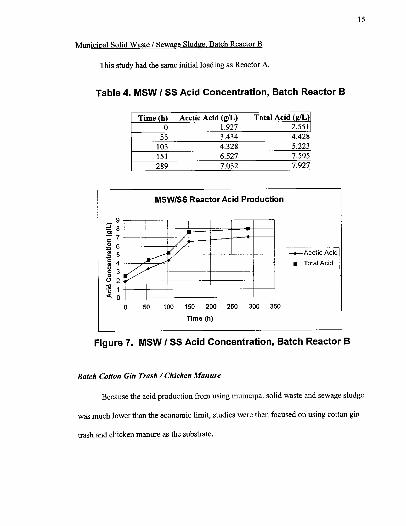
Munici al Solid Waste I Sewa e Slud e Batch Reactor B
This study had the same initial loading as Reactor A.
Table 4. MSW I SS Acid Concentration, Batch Reactor B
Time h Acetic Acid
55 103
1. 927 3. 434 4. 328
Total Acid 2. 551 4. 428 5. 223
151 6. 527 7. 595 289 7. 032 7. 927
MSW/SS Reactor Acid Production
Ol 7 C 0
L. 5 C e 4 — '- c 3 O O D
1
0
0 50 100 150 200 250 300 350
Time (h)
[~ Acetic Acigd
T & I A id
Figure 7. MSW I SS Acid Concentration, Batch Reactor B
Batch Cotton Gin Trash /Chicken Manure
Because the acid production from using municipal solid waste and sewage sludge
was much lower than the economic limit, studies were then focused on using cotton gin
trash and chicken manure as the substrate.
16
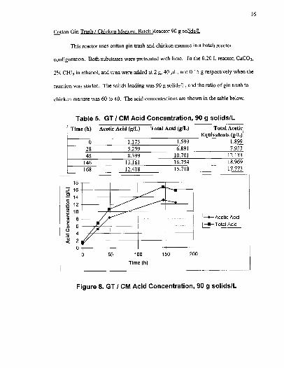
Cotton Gin Trash / Chicken Manure Batch Reactor 90 solids/L
This reactor uses cotton gin trash and chicken manure in a batch reactor
configuration. Both substrates were pretreated with lime. To the 0. 20 L reactor, CaCO&,
2% CHIi in ethanol, and urea were added at 2 g, 40 IiL, and 0. 15 g respectively when the
reaction was started. The solids loading was 90 g solids/L, and the ratio of gin trash to
chicken manure was 60 to 40. The acid concentrations are shown in the table below.
Table 5. GT / CM Acid Concentration, 90 g solids/L
Time (h) Acetic Acid (g/L) Total Acid (g/L) Total Acetic E uivalents
0 1. 175 1. 599 l. 899
28 5. 259 6. 891 7. 953 48 8. 399 10. 701 12. 133
146 168
13. 161 12. 418
16. 754 15. 718
18. 969 17. 773
18
14 ca
C '- 12
10 C
8
o 8 4
2
0 50 100 150 200
Time (h)
'~Acetic Acid
Q~ Total ~Acid
Figure 8. GT / CM Acid Concentration, 90 g solids/L

17
Cotton Gin Trash / Chicken Manure Batch Reactor 200 solids/L
This reactor was similar to the reactor with 90 g solids/L initial loading, the
difference being that the initial solids loading for this reactor was 200 g solids/L for a
reactor volume of 0. 20 L. Acid concentrations are shown in the table below.
Table 6. GT / CM Acid Concentration, 200 g solids/L
Time (h) Acetic Acid (g/L) Total Acid (g/L) Total Acetic E uivalents
0 1. 175 1. 599 1. 899 20 6. 497 9. 231 10. 875
92 8. 872 12. 274 14. 226
122 141
11. 081 12. 385
15. 604 17. 079
18. 223 19. 810
18
16
ta 14
0 12
10 C
8
V 8 6
4
~Acetic Amd ~ Total Acid
50
Time (h)
100 150
Figure 9. GT / CM Acid Concentration, 200 g solids/L

18
Cotton Gin Trash / Chicken Manure Batch Reactor 300 solids/L
This reactor is similar to the previous reactors except for the initial solids loading
of 300 g/L for a reactor volume of 0. 20 L. The acid concentrations are shown below.
Table 7. GT I CM Acid Concentration, 300 g solids/L
Time (h) Acetic Acid (g/L) Total Acid (g/L) Total Acetic E uivalents /L
0 1. 615 2. 845 3. 589 48 8. 214 10. 707 12. 333 84 10. 629 13. 452 15. 272
97 14. 822 18. 849 21. 444
168 193
15. 299 13. 615
19. 451 18. 401
22. 177 21. 455
264 4. 784 10. 514 14. 152
P 20 C 0 e 15
10 0 O
5
0 0 50 100 150 200 250 300
Time (h)
~ Acetic Acid ~ Total Acid
Figure 10. GT I CM Acid Concentration, 300 g solids/L

19
Cotton Gin Trash / Chicken Manure Batch Reactor 350 solids/L
This reactor had an initial solids loading of 350 g/L. The acid concentrations are
shown below.
Table 8. GT/ CM Acid Concentration, 350 g solids/L
Time (h) Acetic Acid (g/L) Total Acid (g/L) Total Acetic E uivalents
0 1. 615 2. 845 3. 589
84 97
168 193
9. 137 10. 674 14. 502 17. 120 16. 335
12. 370 13. 987 18. 917 21. 984 21. 441
14. 479 16. 128 21. 764 25. 057 24. 688
264 7. 770 14. 082 18. 076
25
ce 20 L ct
g 15 a
C o 10 0 o 'Q 5
0 0 50 100 150 200 250 300
Time (h)
~ Acetic Acid ~ Total Aatd
Figure 11. GT / CM Acid Concentration, 350 g solids/L
20
CPDMModeiing using GT/CMBatch Data
The above data shows a decreasing acid concentration atter a seven-day residence
time. The degradation of the acid at the higher temperature probably causes this
reduction. Even though CHIs was added to deter reduction of the product acids to
methane, the initial addition to the reactor is apparently only effective for seven days.
Because of this decreasing concentration, two models were created. One discards data
after the fifth data point. The second model uses all data collected.
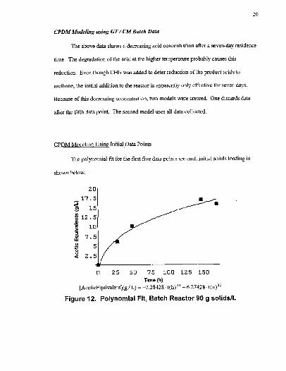
CPDM Modelin Usin Initial Data Points
The polynomial fit for the first five data points are each initial solids loading is
shown below.
20 17. 5
cn 15 c 12. 5
) ~10 7. 5
5 2. 5
0 25 50 75 100 125 150 Time (h)
[AceticEquivalent](g /L) = — 7. 28428 t(h)" + 6. 27428 t(h)"
Figure 12. Polynomial Fit, Batch Reactor 90 g solids/L

21
25
20 8 15
10 8
0 25 50 75 100 125 150 Time (h)
[AceticEquivalent](g /L) = — 226121 t(h)" + 4. 63803 t(h)"
Figure 13. Polynomial Fit, Batch Reactor 200 g solids/L
25
20 8 15
10
u 5
0 25 50 75 100 125 150 Time (h)
[AceticEquivalent](g / L) = — 12. 5402 t(h)" + 8. 71143 t(h)"
Figure 14. Polynomial Fit, Batch Reactor 300 g solids/L
22
25 Ol
g 20 C I
15 Q
10 O
Q 5
0 25 50 75 100 125 150 Time (h)
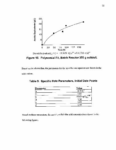
[AceticEquivalent](g /L) = — 13. 3039 t(h)" + 9. 41714. t(h)"
Figure 15. Polynomial Fit, Batch Reactor 350 g solids/L
Based on the above data, the parameters for the specific rate equation are shown in the
table below.
Table 9. Specific Rate Parameters, Initial Data Points
Parameter Value 0. 79 ll l. 00
10. 63 -3. 36 L05 1. 99
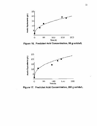
Based on these parameters, the model predicts the acid concentrations shown in the
following figures.
23
25
8 Cl
lO
O IU V
I V
20
15
10
5
0 50 100 150 200 Time (h)
Figure 16. Predicted Acid Concentration, 90 g solids/L
8 O Ilj
0 UJ
s 4l
25
20
15
10
5
50 100 150 200 Time (h)
Figure 17. Predicted Acid Concentration, 200 g solids/L
8 Cl
EO
0 Lu O
Cl V
25
20
15
10
5
0 50 100 150 200 Time (h)
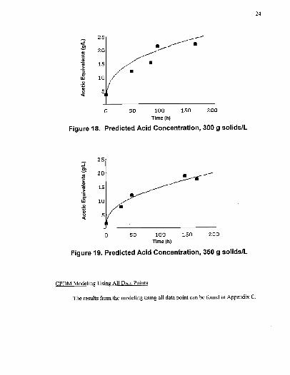
Figure 18. Predicted Acid Concentration, 300 g solids/L
8 O Ill
rr Lu
V
CO V
25
20
15
10
5
0 50 100 150 200 Time (h)
Figure 19. Predicted Acid Concentration, 350 g solids/L
CPDM Modelin Usin All Data Points
The results from the modeling using all data point can be found in Appendix C.
25
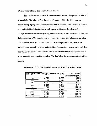
Couniercurrenr Corron Gin Trash/Chicken Manure
Three reactors were operated in a countercurrent process. The procedure is listed
Appendix D, The solids loading for the set of reactors is 288 g/L. This value was
determined by drying a sample to determine the water content. Then the fraction of solids
was multiplied by the kept weight in each reactor to determine the solids loading.
Though the reactors have been operating countercurrently, recently discovered differences
in interpretations of the procedure have prevented the system from attaining steady state.
The procedure states that the reactors should be centrifuged before the contents are
moved countercurrently. Another method of transfer prescribes two successive centrifuge
and transfer procedures. This alternate method will result is a different liquid residence
time, upon which the model is dependent. The data below show the transient state of the
system.
Table 10. GT I CM Acid Concentration, Countercurrent
Time (h) Acetic Acid (g/L) Total Acid (g/L) Total Acetic E uivalents /L
0 0. 326 2. 796 4. 066 48 96
144
2. 486 5. 611 7. 363 0. 963 3. 709 5. 288 2. 727 6. 498 8. 737
192 7. 828 12. 833 15. 898 288 336 384 432
1. 995 6. 112 8. 649 2. 997 5. 480 7. 016 6. 103 9. 076 10. 859 6. 162 10. 312 12. 843

26
14
12
10 0
Q
0 o 4
2
~Acetic Acid ~ Total Acid
0 50 100 150 200 250 300 350 400 450 500
Time (h)
Figure 20. GT I CM Acid Concentration, Countercurrent
Therefore, data are not available to compare against the modeling done with the batch
systems.

27
Results and Conclusions
The bacteria cultures produce acids from the gin trash and chicken manure
substrate in greater amounts than municipal solid waste and sewage sludge at
thermophilic conditions. However, these acids quicldy decompose because of the higher
temperatures. In order to maximize acid production, liquid residence times should be
limited to seven days. With limited liquid residence times, the acids will be removed
from the system before degradation begins to offset new acid production. An alternative
to shorter residence times would be periodic addition of iodo form to the system. Data
indicates that iodoform inhibits the reduction of product acids to methane initially;
however, by continuously adding iodoform, the effectiveness may be extended beyond
seven days.
Reactor failure was a factor in limited data collected. Due to safety concerns,
glass containers are not used. The polyproplyene reactor bottles quickly deform when
placed under pressure at elevated temperatures. Not only is there gas produced from the
reaction, but the because of the thermophilic temperatures, the gas law predicts a higher
pressure for a given volume. Though experiments show that diffusion is not a concern
with these reactors, pressure cannot be allowed to build up. The reactors must be vented
daily to minimize pressure. Further studies should be done to determine the effect of
creating a vacuum within the confiner before returning the reactor to the air bath. With
less initial gas in the reactor, the pressure should increase at a slower rate.
Also, as expected, a higher initial solids loading leads to higher acid
concentrations. The CPDM method when applied to cotton gin hash and chicken
manure accurately predicts acid production. More data should be taken in further studies

28
to better refine the model. Also, the countercurrent system should be allowed to reach
steady state in order to verify the model against experimental data.
The model was extended to data for multiple reactors with different numbers of
data points. The Mathematica input files are listed in the Appendix B and Appendix C.
The inputs files for the model utilizing All Data Points include revisions to handle data
sets with different numbers of data points.
In conclusion, the data collected by this study indicates that an industrial scale
process using cotton gin trash and chicken manure as the substrate for the MixAIco
process could be economical.

29
Literature Cited
Chang, V. S. , B. Burr, and M. T. Holtzapple, Lime Pretreatment of Switchgrass,
Manuscript, Chemical Engineering Department, Texas AbtM University.
Cheremisinoff, N. P. , P. N. Cheremisinoff, and F. Efferbusch, Biomass: Applications,
Technology, and Production, Marcel Dekker, New York (1980).
France, J. and R. C. Siddons, "Volatile Fatty Acid Production, " in Quantitative Aspects of Ruminant Digestion and Metabolism, J. M. Forbes and J. France, eds. , CAB International, Wallingford, UK (1993).
Loescher, M. E. , "Volatile Fatty Acid Fermentation of Biomass and Kinetic Modeling
Using the CPDM Method", PhD Dissertation, Texas AbbM University, College Station, TX (1996).
McCarty, P. L. , "One Hundred Years of Anaerobic Treatment, " in Anaerobic Digestion
1981, D. E. Hughes, D. A. Stafford, B. I. Wheatley, W. Baader, G. Lettinga, E. J. Nyns, W. Verstraete, and R. L. Wentworth, eds. , Elsevier Biomedical, Amsterdam
(1982).
Rapier, C. R. , "Volatile Fatty Acid Fermentation of Lime-treated Biomass by Rumen
Microorganisms", MS thesis, Texas AkM University, College Station, TX (1995).
Zehnder, A. J. B. , K. Ingvorsen, and T. Marti, "Microbiology of Methane Bacteria, " in
Anaerobic Digestion 1981, D. E. Hughes, D. A. Stafford, B. I. Wheatley, W. Baader, G. Lettinga, E. J. Nyns, W. Verstraete, and R. L, Wentworth, eds. , Elsevier Biomedical, Amsterdam (1982).

30
Appendix
A. Fall Data Sets
All acid concentrations given in (g/L).
Munici al Solid Waste / Sewa e Slud e Batch Reactor A
Time h Acetic Pro ionic Bu ric Valeric Other Total AcE 0 2909 0. 412 0. 240 0. 145 0. 260 3. 966 4. 722
24 51 73
139 163 192 218 266 283 314 332
3. 498 3. 825 3. 851 3. 957 4. 262 4. 516 4. 553 4. 787 4. 713 5. 396 5. 396
0. 460 0. 483 0. 384 0. 156 0. 149 0. 135 0. 116 0. 107 0. 098 0. 054 0. 063
0. 273 0. 304 0. 276 0. 211 0. 214 0. 225 0. 227 0. 230 0. 226 0. 251 0. 260
0. 183 0. 186 0. 154 0. 103 0. 102 0. 115 0. 117 0. 133 0. 126 0. 155 0. 167
0. 147 0. 155 0. 124 0. 037 0. 016 0. 023 0. 026 0. 027 0. 039 0. 075 0. 075
4. 561 5. 270 4. 954 5. 707 4. 789 5. 417 4. 464 4. 813 4. 743 5. 067 5. 014 5. 359 5. 039 5. 384 5. 285 5. 644 5. 203 5. 563 5. 931 6. 359 5. 961 6. 410
Munici al Solid Waste / Sewa e Slud e Batch Reactor B
Time h Acetic Pro ionic Bu ric Valeric Other Total AcK
0 1. 927 0. 242 0. 234 0. 122 0. 025 2. 551 2. 956
55 103 151 289
3. 434 4. 328 6. 527 7. 032
0. 360 0. 314 0. 381 0. 251
0. 362 0. 349 0. 398 0. 388
0. 228 0. 184 0. 193 0. 203
0. 043 0. 048 0. 096 0. 052
4. 428 5. 089 5. 223 5. 820 7, 595 8. 321 7. 927 8. 548
Cotton Gin Trash / Chicken Manure 90 solids/L
Time h Acetic Pro ionic Bu ric Valeric Other Total AcK
0 1. 175 0, 093 0. 204 0. 113 0. 014 1. 599 1. 899 28 48
146 168
5. 259 8. 399
13. 161 12. 418
0. 570 0. 924 1. 473 1. 303
0. 752 1. 061 1. 665 1. 551
0. 257 0. 272 0. 388 0. 379
0. 053 0. 046 0. 067 0. 067
6. 891 7. 953 10. 701 12. 133 16. 754 18. 969 15. 718 17. 773
31
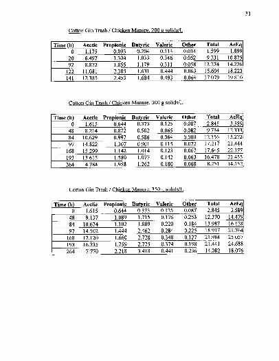
Cotton Gin Trash / Chicken Manure 200 solids/L
Time h Acetic Pro ionic Bu ric Valeric Other Total AcE 0 1. 175 0. 093 0. 204 0. 113 0. 014 1. 599 1. 899
20 92
122 141
6. 497 8. 872
11. 081 12. 385
1. 304 1. 855 2. 385 2. 453
1. 033 1. 179 1. 631 1. 684
0. 346 0. 311 0. 444 0. 493
0. 052 0. 058 0. 063 0. 064
9. 231 12, 274 15. 604 17. 079
10. 875 14. 226 18. 223 19. 810
Cotton Gin Trash / Chicken Manure 300 solids/L
Time h Acetic Pro ionic Bu ric Valeric Other Total AcE 0 1. 615 0. 644 0. 373 0. 125 0. 087 2. 845 3. 589
48 84 97
168 193 264
8. 214 10. 629 14. 822 15. 299 13. 615 4. 784
0. 872 0. 997 1. 307 1. 142 1. 580 1. 958
0. 502 0. 586 0. 901 l. 014 1. 077 1. 262
0. 065 0. 064 0. 115 0. 123 0. 142 0. 180
0. 082 0. 080 0. 072 0. 067 0. 063 0. 068
9. 734 12. 356 17. 217 17. 645 16. 478 8. 251
12. 333 15. 272 21. 444 22. 177 21. 455 14. 152
Cotton Gin Trash / Chicken Manure 350 solids/L
Time h Acetic Pro ionic Bu ric Valeric Other Total AcE 0 1. 615 0. 644 0. 373 0. 125 0. 087 2. 845 3. 589
48 84 97
168 193 264
9. 137 10. 674 14. 502 17. 120 16. 335 7. 770
1. 089 1. 102 1. 444 1. 660 1. 759 2, 218
1. 715 1. 809 2. 462 2. 728 2. 775 3. 418
0. 176 0. 220 0. 284 0. 348 0. 374 0. 441
0. 253 0. 184 0. 225 0. 127 0. 198 0. 236
12. 370 13. 987 18. 917 21. 984 21. 441 14. 082
14. 479 16. 128 21. 764 25. 057 24. 688 18. 076

32
Cotton Gin Trash / Chicken Manure Countercurrent
Time h Acetic Pro ionic Bu ric Valeric Other Total AcE 0 0. 326 2. 009 0. 079 0. 269 0. 113 2. 796 4. 066
48 2. 486 2. 095 0. 474 0. 394 0. 162 5. 611 7. 363 96 0. 963 1. 711 0. 563 0. 279 0. 194 3. 709 5. 288
144 2. 727 2. 202 0. 747 0. 571 0. 250 6. 498 8. 737 192 7. 828 2. 446 1. 651 0. 616 0. 292 12. 833 15. 898 288 1. 995 1. 856 1. 598 0. 487 0. 176 6. 112 8. 649 336 2. 997 1. 161 0. 905 0. 252 0. 164 5. 480 7. 016 384 6. 103 1. 515 1. 051 0. 220 0. 1 85 9. 076 10. 859 432 6. 162 1. 915 1. 701 0. 307 0. 226 10. 312 12. 843
33
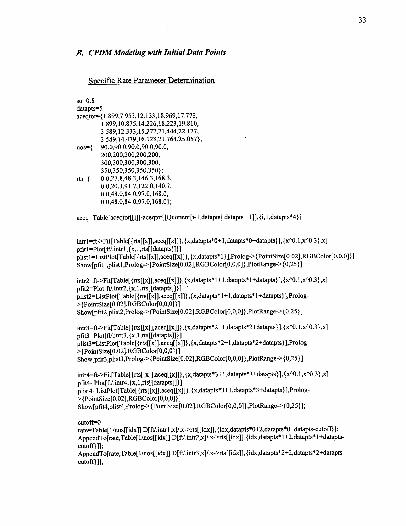
B. CPDM Modeling with Initial Data Points
S ecific Rate Parameter Determination
so=0. 8 datapts=5 aceqtot= {1. 899, 7. 953, 12. 133, 18. 969, 17. 773,
1. 899, 10. 875, 14. 226, 18. 223, 19. 810, 3. 589, 12. 333, 15. 272, 21. 444, 22. 177, 3. 589, 14. 479, 16. 128, 21. 764, 25. 057);
nos={ 90, 0, 90. 0, 90. 0, 90. 0, 90. 0, 200, 200, 200, 200, 200, 300, 300, 300, 300, 300, 350, 350, 350, 350, 350);
rts=( 0. 0, 27. 8, 48. 3, 146. 3, 168. 3, 0. 0, 20. 3, 91. 7, 122. 0, 140. 7, 0. 0, 48. 0, 84. 0, 97. 0, 168. 0, 0. 0, 48. 0, 84. 0, 97. 0, 168. 0);
aceq=Tabfe[aceqtot[[i]]-aceqtot[[Quotient[i-l, datapts] datapts+1]], {i, l, datapts'4)]
intrl=ft-&Fit[Tabfe[{rts[[x]], aceq[[x]]}, (x, datapts'0+t, datapts*0+datapts}], {x'%. 1, x 0. 3), x] pfit 1 =Plot[fU. intr 1, (x, l, rts[[datapts]])] plist1 =ListPlot[Table[{rts[[x]], aceq[[x]]), (x, datapts* 1 ) ], Prolog-& {PointSize[0. 02], RGBColor[0, 0, 0]) ] Show[pfitl, plist1, Prolog-& {PointSize[0. 02], RGBColor[0, 0, 0]}, PlotRange-&(0, 25}]
intr2=f1-&Fit[Table[(rts[[x]], aceq[[x]]}, {x, datapts'1+1, datapts*l+datapts)], {x O. l, x"0. 3), x] pfit2=Plot[f1/. intr2, (x, l, rts[[datapts]]) ] plist2=ListPlot[Table[(rts[[x]], aceq[[x]]), (x, datapts'1+1, datapts*l+datapts}], Prolog- & {PointSize[0. 02], RGBColor[0, 0, 0]}] Show[pfit2, plist2, Prolog-& {PointSize[0. 02], RGB Color[0, 0, 0]), PlotRange-& {0, 25) ]
intr3=f1-& Fit [Tab le [{rts [(x]], aceq[[x]] ), {x, datapts'2+ 1, datapts'2+datapts} ], (x "0. l, x 0. 3), x] pfit3=Plot[fU. intr3, (x, l, rts[[datapts]]) ] pl ist3=Lis tP lot[Table [(rts [[x]], aceq[[x]] ), (x, dataptss2+ 1, datapts'2+datapts}], Prolog- & {PointSize[0. 02], RGBColor[0, 0, 0]}] Show[pgtt3, plist3, Prolog-& (PointSize[0. 02], RGBColor[0, 0, 0]}, PlotRange-&(0, 25)]
intr4=f1-&Fit[Table[ {rts[[x]], aceq[[x]]}, (x, datapts*3+1, datapts'3+datapts)], (x"O. l, x'0. 3), x] pfit4=P lot[f1/. intr4, (x, l, rts [[datapts]]) ] plist4=Listplot[Table[(rts[[x]], aceq[[x]]), {x, dataptss3+1, datapts" 3+datapts)], prolog-
&{PointSize[0. 02], RGBColor[0, 0, 0])] Show[pfit4, plist4, Prolog-& {PointSize[0. 02], RGBColor[0, 0, 0]), PlotRange-& { 0, 25) ]',
cutoff=0 rate=Table[1/nos[[idx]] D[fU. intr 1, x]/. x-&rts[[idx]], (idx, datapts*0+2, dataptse0+datapts-cutoff) ]; AppendTo[rate, Table[1/nos[[idx]] D[fi/. intr2, x]/. x-&rts[[idx]], (idx, datapts" 1+2, datapts*l+datapts-
cutoff) ]]; AppendTo[rate, Table[1/nos[[idx]] D[fl/. intr3, x]/. x-&rts[[idx]], (idx, datapts*2+2, dstapts'2+datapts-
cutoff} ]];

34
AppendTo[rate, Table[1/nos[[idx]] D[ff/. intr4, x]/. x-&rts[[idx]], (idx, datapts'3+2, datapts'3+datapts-
cutoff) ]]; rate=Flatten[rate];
xes= Table[If[(aceqf[idx]]/so/nos[[idx]])&1, 0. 999, (aceq[[idx]])/so/(nos[[idx]])], (idx, datapts'0+2, dataptsa0
+data pts-cutoff) ]; AppendTo[xes, Table[if[(aceq[[idx]]/so/nos[[idx]])&1, 0. 999, (aceq[[idx]])/so/(nos[[idx]])], (idx, datapts*1+2,
datapts s I+datapts-cutoff} ]]; AppendTo[xes, Table[If[(aceq[[idx]]/so/nos[[idx]])&1, 0. 999, (aceq[[idx]])/so/(nos[[idx]])], (idx, datapts'2+2,
datapts "2+datapts-cutoff) ]]; AppendTo[xes, Table[If[(aceq[[idx]]/so/nos[[idx]])&1, 0. 999, (aceq[[idx]])/so/(nos[[idx]])], (idx, datapts'3+2,
datapts~3+datapts-cutoff}]]; xes=Flatten[xes];
aces= Tab le [ac eqtot[[idx]], (idx, datapts "0+2, datapts*o+datapts-cutoff} ]; AppendTo[aces, Table[aceqtot[[idx]], (idx, dataptsa 1+2, datapts*l+datapts-cutoff}]];
AppendTo[aces, Table[aceqtot[[idx]], (idx, datapts'2+2, datapts'2+datapts-cutoff}]];
AppendTo [aces, Tab le [aceqtot[[idx]], {idx, datapts '3+2, datapts *3+ datapts-cutoff} ]]; aces=Flatten[aces];
rmodel[x, ac J:=a(l-x) d/(I+b(x) e+c ac~f)
fit=FindMinimum[Sum[(rate[[idx]]-rmodel[xes[[idx]], aces[[idx]]]) 2, {idx, l, (datapts-l-
cutoff)*4}], {a3, 0, 30}, {b, 1, -100, 100), (c, 10, -1000, 1000}, (e, 1. 05, 0, 1000}, {f 1. 20, 1000}, {d, 1. 2, -
50, 1000 }, Maxlter ations-& 100000]
totalen=Sum[rate[[idx]] "2, (idx, 1, (datapts-l-cutoff)*4 }]
pctfit=100-(fit[[1]]/totalerr)" 100
rmodel[x, ac]/. fit[[2]]
Plot3 D[rmodel[x, ac]/. fit[[2]], {x, 0, . 95), (ac, 0, 20}, Viewpoint-& (2. 442, 5. 268, 1. 970), PlotRange-
&(0, . 25 }, PlotPoints-&40]
Batch Reactor Simulation
so=0. 8 rmodel[x acJ:=a(I-x) d/(I+b(x) e+c ac f) rmode 1 [x, ac]
fit=(1. 75877 IOE-7, (a -& 0. 793308, b -& 1. 00032, c -& 10. 6326, e -& 1, 04829, f'-& 1. 99275, d -& -3, 36335})
datapts=5
aceqtot= { l. 899, 7. 953, 12. 133, 18. 969, 17. 773, 1. 899, 10. 875, 14. 226, 18. 223, 19. 810, 3. 589, 12. 333, 15. 272, 21. 444, 22. 177, 3. 589, 14. 479, 16. 128, 21. 764, 25. 057 };
nos={ 90. 0, 90. 0, 90. 0, 90. 0, 90. 0, 200, 200, 200, 200, 200,

35
300, 300, 300, 300, 300, 350, 350, 350, 350, 350); 0. 0, 27. 8, 48. 3, 146. 3, 168. 3, 0. 0, 20. 3, 91. 7, 122. 0, 140. 7, 0. 0, 48. 0, 84. 0, 97. 0, 168. 0, 0. 0, 48. 0, 84. 0, 97. 0, 168. 0);
run= 1; nos[[(run-1)edatapts+1]] aceqtot[[(run-1) edatapts+1]]
nos[[(nm-1)adatapts+1]] rmodel[(aceqtot[[(run-1)'datapts+1]]-aceqtot[[(run-1) *datapts+1]])/
(so nos[[(run-1)*datapts+1]]), aceqtot[[(run-1)*datapts+1]]]/. fit[[2]]
ans=NDSolve[{ acid'[t]=~os[[(run-1)'datapts+1]] rmodel[(acid[t]-aceqtot[[(run-1)*datapts+1]])/
(so nos[[(run-1) "datapts+1]]), acid[t]]/. fit[[2]], acid[0]==aceqtot[[(run-1)*datapts+1]]),
acid [t], (t, 0, 200) ]
pl =Plot[acid[t]/. ans, (t, 0, 200), PlotRange-&(0, 25) ] p 1 dat=ListPlot[Table[ {rts[[(run-1)'datapts+i]], aceqtot[[(run-l )*datapts+i]] }, (i, l, datapts}]] Show [p l, p 1 dat, Prolog-& {PointSize[0. 02], RGB Color[0, 0, 0]), PlotRange-& {0, 25) ]
rtm=2; nos[[(run-1)*datapts+1]] aceqtot[[(run-1)" datapts+1]]
nos[[(rum-1) vdatapts+1]] rmodel[(aceqtot[[(run-1)*datapts+1]]-aceqtot[[(run-1)" datapts+1]])/
(so nos[[(rum-1)edatapts+1]]), aceqtot[[(run-1)'datapts+1]]]/. fit[[2]]
ans=NDSolve[{ acid'[t] — ~os[[(run-1)*datapts+1]] rmodel[(acid[t]-aceqtot[[(run-1)adatapts+1]])/
(so nos[[(run-1)'datapts+1]]), acid[t]]/. fit[[2]], acid[0]==aceqtot[[(run-1)"datapts+1]]), acid[t], {t, 0, 200)]
p2=Plot[acid[t]/, ans, (t, 0, 200), PlotRange-&{0, 25 } ] p2dat=ListPlot[Table[{rts[[(run-1)*datapts+i]], aceqtot[[(run- 1) adatapts+i]] }, {i, l, datapts)]] Show [p2, p2dat, Prolog-&(PointSize[0. 02], RGBColor[0, 0, 0]), PlotRange-&{0, 25}]
full=3; nos[[(run-1)*datapts+1]] aceqtot[[(run-1) "datapts+1]]
nos[[(run-1)" datapts+1]] rmodel[(aceqtot[[(run-1)'datapts+1]]-aceqtot[[(run-1)'datapts+1]])/ (so nos[[(run-1)*datapts+1]]), aceqtot[[(run-1)'datapts+1]]]/. fit[[2]]
ans=NDSolve[( acid'[t]==nos[[(run-1)*datapts+1]] rmodel[(acid[t]-aceqtot[[(run-l)*datapts+1]])/
(so nos[[(run-1)'datapts+1]]), acid[t]]/. fit[[2]], acid[0]==aceqtot[[(run-1)"datapts+1]]), acid[t], {t, 0, 200) ]
p3=P lot[acid [t]/. ans, (t, 0, 200), PlotRange-& { 0, 25 } ]
36
p3dat=Listplot[Table[{rts[[(run- I)'datapts+i]], aceqtot[[(run-l)sdatapts+i]] ), { i, l, datapts) ]] Show [p3, p3dat, Prolog-& {PointSize[0. 02], RGBColor[0, 0, 0]), PlotRange-& {0, 25) ]
run=4; nos[[(run-I)" datapts+ I]] aceqtot[[(run-I) sdatapts+ I]]
nos [[(run-1)*datapts+I]] rmodel[(aceqtot[[(run- I)'datapts+ I]]-aceqtot[[(run-1)*datapts+ I ]])/ (so nos[[(run-I)'datapts+I]]), aceqtot[[(run-I)*datapts+I]]]/. fit[[2]]
ans=NDSolve[{ acid'[t]=~os[[(run-I)'datapts+I]] rmodel[(acid[t]-aceqtot[[(run-I)'datapts+I]])/ (so nos[[(run-I)'datapts+I]]), acid[t]]/. fit[[2]], acid[0]==aceqtot[[(run-1)*datapts+I]]), acid[t], {t, 0, 200) ]
p4=Plot [ac id[t]/. ans, {t, 0, 200), PlotRange-& { 0, 25) ] p4dat=ListPlot[Table[{rts[[(run-I)"datapts+i]], aceqtot[[(run-l)*datapts+i]]), {i, l, datapts)]] Show [pi, p 1dat, Prolog-& {PointSize[0. 02], RGBColor[0, 0, 0]), PlotRange-&{0, 25)]

37
C. CPDM Modeling with All Dala Points
S ecific Rate Parameter Determination
so=0. 8 datapts=7 ace qtot= ( l. 899, 7. 95 3, 12. 133, 18. 969, 17. 773, 0, 0,
1. 899, 10. 875, 14. 226, 18. 223, 19. 810, 0, 0, 3. 589, 12. 333, 15. 272, 21. 444, 22. 177, 21. 455, 14. 152, 3. 589, 14. 479, 16. 128, 21. 764, 25. 057, 24. 688, 18. 076);
nos=( 90. 0, 90. 0, 90. 0, 90. 0, 90. 0, 90. 0, 90. 0, 200, 200, 200, 200, 200, 200, 200, 300, 300, 300, 300, 300, 300, 300, 350, 350, 350, 350, 350, 350, 350};
rts=( 0. 0, 27. 8, 48. 3, 146. 3, 168, 3, 0, 0, 0. 0, 20. 3, 91. 7, 122. 0, 140. 7, 0, 0, 0. 0, 48. 0, 84. 0, 97. 0, 168. 0, 193. 0, 264. 0, 0. 0, 48. 0, 84. 0, 97. 0, 168. 0, 193. 0, 264. 0};
ace q= Tab le [ac eqtot[[i]]-aceqtot [[Quotient [i- l, datapts] datapts +1]], { i, l, datapts'4 } ]
intr 1 =it-&Fit[Table[(rts[[x]], aceq[[x]]), (x, datapts*0+1, datapts "0+datapts-2}], (x"O. l, x 0. 3 }, x]
pfit1 =plot[RJ. intr 1, (x, l, rts[[datapts'0+datapts-2]]) ] plistl=ListPlot[Table[(rts[[x]], aceq[[x]]}, {x, datapts*1-2)], Prolog-& (PointSize[0. 02],
RGBColor[0, 0, 0])] Show[pfitl, plist 1, Prolog-& {PointSize[0. 02], RGBColor[0, 0, 0] }, PlotRange-&(-10, 20 }]
intr2=R-&F it[Table[ {rts[[x]], aceq[[x]]), (x, datapts* 1+ 1, datapts'1+datapts-2 }], { x"0. l, x"0. 3 }, x]
pfiQ=P tot [R/. ht tr2, (x, I, rts[[datapts" 1+datapts-2]]) ] plist2=ListPlot[Table[{rts[[x]], aceq[[x]]), {x, datapts*l+Ldataptssl+datapts-2)],
Prolog-& (P oint Size [0. 02], RGB Color[0, 0, 0] ) ] Show[pftQ, plisQ, Prolog-&(PointSize[0. 02], RGBColor[0, 0, 0]), PlotRange-& (-10, 20) ]
intr3=R-&Fit[Table[(rts[[x]], aceq[[x]]), {x, datapts "2+ 1, datapts" 2+datapts}],
{x O. l, x'0. 3}, x] pfit3=plot[fU. intr3, {x, l, rts[[dataptss2+datapts]]} ] pl ist3 =ListPlot[Table [ {rts[[x]], aceq[[x]]), {x, datapts *2+ l, dataptse2+datapts } ],
Prolog-& {PointSize[0. 02], RGBColor[0, 0, 0]}] Show[pfit3, plist3, Prolog-&(PointSize[0. 02], RGBColor[0, 0, 0]}, PlotRange-&(-10, 20}]
intr4=R-&Fit[Table[(rts[[x]], aceq[[x]] }, {x, datapts*3+ Ldatapts'3+datapts) ], (x O. l, x"0. 3), x]
pfit4=P lot [ft/. intr4, (x, l, rts [[datapts*3+datapts]] } ] plist4=ListPlot[Table[(rts[[x]], aceq[[x]]), (x, datapts" 3+ 1, datapts'3+datapts) ],
Prolog-&(PointSize[0. 02], RGB Color[0, 0, 0] }] Showgfit4, plist4, prolog-&{PointSize[0. 02], RGBColor[0, 0, 0]), PlotRange-& {-10, 20) ];

38
cutoff'=0
rate=Table[1/nos[[idx]] D[ff/. intrl, x]/. x-&rts[[idx]], {idx, datapts'0+2, datapts'0+ datapts-cutoff-2 }];
AppendTo[rate, Table[1/nos[[idx]] D[ff/. intr2, x]/. x-&rts[[idx]], (idx, datapts" 1+2, dataptss I+datapts-cutoff-2) ]];
Appear}To[rate, Table[1/nos[[tdx]] D[ft/. mtr3, x]/ x-&rts[[rdxl], ( tdx d»p&' + datapts'r2+datapts-cutoff}]];
AppendTo[rate, Table[1/nos[[idx]] D[ff/. intr4, x]/. x-&rts[[idx]], {idx, datapts*3+2, datapts'3+datapts-cutoff) ]];
rate=Flatten[rate];
xes= Table [If[(aceq[[idx]]/so/nos[[idx]])&1, 0. 999, (aceq[[idx]])/so/(nos[[idx]])],
{ idx, datapts s 0+2, datapts*o+datapts-cutoff-2) ]; AppendTo[xes, Table[If[(aceq[[idx]]/so/nos[[idx]])&1, 0. 999, (aceq[[idx]])/so/
(nos [[i dx]])], (idx, datapts" 1+2, d ate pts* 1+de tap ts-cutoff'-2}]], '
AppendTo[xes, Table[If[(aceq[[idx]]/so/nos[[idx]])&1, 0. 999, (aceq[[idx]])/so/ (nos[[idx]])], (idx, datapts"2+2, datapts*2+datapts-cutoff)]];
Append To [xes, Table[If[(aceq [[i dx]]/so/nos[[idx]])& 1, 0. 999, (ace q[[idx]])/so/ (nos[[idx]])], (idx, datapts*3+2, datapts'3+datapts-cutoff}]];
xes=Flatten[xes];
aces= Table [aceqtot[[idx]], {idx, datapts'0+2, datapts*o+datapts-cutoff-2 }]; AppendTo[aces, Table[aceqtot[[idx]], (idx, datapts*1+2, datapts*l+datapts-cutoff 2}]]; Append To [aces, Table [aceqtot[ [idx]], { idx, d atapts" 2+2, datapts *2+ datapts-cutoff} ]]; AppendTo[aces, Table[aceqtot[[idx]], (idx, datapts*3+2, dataptsr3+datapts-cutoff)]]; aces=Flatten[aces];
rmodel[x, ac J:=a(l-x) d/(1+b(x)ee+c ac"f)
fit=FindMinimum[ Sum[(rate[[idx]]-rmodel[xes[[idx]], aces[[idx]]])"2, { idx, 1, (datapts -I-cutoff)" 4-(2)'2)], (a, 3, 0, 50), {b, 5, -100, 100), (c, 10, -1000, 1000 }, (e, 1. 5, 0, 1000), {f, 1. 8, 0, 1000}, {d, 1, -10, 1000}, Maxlterations-&100000]
totalerr — Sum[rate[[idx]] "2, {idx, 1, (datapts-l -cutoff) "4-(2)*2) ]
pctfrt=100-(fit[[1]]/totalerr)" 100
rmodel[x, ac]/. ftt[[2]]
Plot3D[rmodel[x, ac]/. fit[[2]], {x, 0, . 95), (ac, 0, 20), ViewPoint-& {2. 442, 5. 268, 1. 970), PlotRange-& (0, 1 }, PlotPoints-&40]
Batch Reactor Simulation
so=0. 8
rmodel[x acJ:=a(1-x)"d/(I+b(x) e+cac f) nnodel[x, ac]
fit= {2. 05831 10~-7, {a -& 4. 95245, b -& 4. 99923, c -& 9. 44343, e -& 1. 50789, f-& 3. 10472, d -& -8. 64968})
39
fit= {2. 56243 10E-7, {a -& 4. 1404, b -& 4. 99923, c -& 9. 97744, e -& 1. 50701, f-& 3. 01889, d -& -8. 82503})
datapts=7
aceqtot={1. 899, 7. 953, 12. 133, 18. 969, 17. 773, 0, 0, 1. 899, 1 b. 875, 14. 226, 18. 223, 19. 810, 0, 0, 3. 589, 12. 333, 15. 272, 21. 444, 22. 177, 21. 455, 14. 152, 3. 589, 14. 479, 16. 128, 21, 764, 25. 057, 24. 688, 18. 076);
nos={ 90. 0, 90. 0, 90. 0, 90. 0, 90. 0, 90. 0, 90. 0, 200, 200, 200, 200, 200, 200, 200, 300, 300, 300, 300, 300, 300, 300, 350, 350, 350, 350, 350, 350, 350);
its={ 0. 0, 27. 8, 48. 3, 146. 3, 168. 3, 0, 0, 0. 0, 20. 3, 91. 7, 122. 0, 140. 7, 0, 0, 0. 0, 48. 0, 84. 0, 97. 0, 168. 0, 193. 0, 264. 0, 0. 0, 48. 0, 84. 0, 97. 0, 168. 0, 193. 0, 264. 0);
run= 1; nos[[(run-1)" datapts+1]] aceqtot[[(run-1) "datapts+1]]
nos[[(run-l)*datapts+1]] rmodel[(aceqtot[[(run-1)" datapts+1]]-aceqtot[[(run-1) 'datapts+1]])/(so nos[[(run-1)"datapts+1]]), aceqtot[[(run-1)a datapts+1]]]/. fit[[2]]
ans=NDSolve[{ acid'[t]~os[[(run-1)"datapts+1]] rmodel[(acid[t]-aceqtot[[(run-1)*
datapts+1]])/(so nos[[(run-1)adatapts+1]]), acid[t]]/. fit[[2]], acid[0]=aceqtot[[(run-1)'datapts+1]]}, acid[t], {t, 0, 200}]
p1=Plot[acid[t]/. ans, {t, 0, 200}, PlotRange-&(0, 25) ] pl dat=Listplot[Table[{Ns[[(run-1)sdatapts+i]], aceqtot[[(run-l)*datapts+i]]},
(i, l, datapts-2 } ]] Show [p l, p 1 dat, Prolog-& { P oint Size [0. 02], RGB Color[0, 0, 0] }, PlotRange-& { 0, 25 } ]
roll=2; nos[[(run-1)'datapts+1]] aceqtot[[(run-1)*datapts+1]]
nos[[(run-1)adatapts+1]] rmodel[(aceqtot[[(run-1)*datapts+1]]-aceqtot[[(run-1) adatapts+1]])/(so nos[[(run-1)'datapts+1]]), aceqtot[[(run-1)' datapts+1]]]/. fit[[2]]
ans=NDSolve[{ acid'[t]==nos[[(run-1)*datapts+1]] rmodel[(acid[t]-aceqtot[[(run-1)' datapts+1]])/(so nos[[(run-1) "datapts+1]]), acid[t]]/, fit[[2]], acid[0]==aceqtot[[(run-1)sdatapts+1]]}, acid[t], {t, 0, 200)]
p2=Plot[acid[t]/. ans, (t, 0, 200), PlotRange-& {0, 25)] p2dat=ListPlot[Table[{rts[[(run-1)"datapts+i]], aceqtot[[(run-l)*datapts+i]]),
40
(LLd tapm-»H Show [p2, p2dat, Prolog-& {PointSize[0. 02], RGBColor[0, 0, 0]), PlotRange-&(0, 25) ]
nrl1=3; nos[[(run-1)sdatapts+1]] aceqtot[[(run-1) sdatapts+1]]
nos[[(run-1)'datapts+1]] rmodel[(aceqtot[[(run-1)"datapts+1]]-aceqtot[[(run-1) 'datapts+1]])/(so nos[[(run-1)"datapts+1]]), aceqtot[[(run-1)' datapts+1]]]/. fit[[2]]
ans=NDSolve[{ acid'[t]==nos[[(run-1)*datapts+1]] rmodel[(acid[t]-aceqtot[[(run-1)*
datapts+1]])/(so nos[[(run-1)'datapts+1]]), acid[t]]/. fit[[2]], acid[0]==aceqtot[[(run-1)*datapts+1]]}, acid[t], {t, 0, 300}]
p3=Plot[acid[t]/. ans, (t, 0, 300), PlotRange-&(0, 25) ] p3dat=Listplot[Table[{rts[[(run-1)"datapts+i]], aceqtot[[(run-l)sdatapts+i]]),
{i, i, datapts}]] Show [p3, p3dat, Prolog-&(PointSize[0. 02], RGBColor[0, 0, 0]), PlotRange-& {0, 25}]
run=4; nos [[(run-1)sdatapts+1]] aceqtot[[(run-1)*datapts+1]]
nos[[(run-1)*datapts+1]] rmodel[(aceqtot[[(run-1)'datapts+1]]-aceqtot[[(run-1) 'datapts+1]])/(so nos[[(run-1)'datapts+1]]), aceqtot[[(run-1)s
datapts+1]]]/. fit[[2]]
ans=NDSolve[{ acid'[t]~os[[(run-1)'datapts+1]] rmodel[(acid[t]-aceqtot[[(run-1)*
datapts+1]])/(so nos[[(run-1)*datapts+1]]), acid[t]]/. frt[[2]], acid[0]=aceqtot[[(run-1)sdatapts+1]]}, acid[t], (t, 0, 300)]
p4=P lot [ac id [t]/. ans, { t, 0, 300), PlotRange-& (0, 25 } ] p4dat=ListPlot[Table [ {rts[[(run-1)" datapts+i]], aceqtot[[(run-l)" datapts+i]]),
(i, l, datapts)]] Show [p4, p4dat, Prolog-&(PointSize[0. 02], RGBColor[0, 0, 0]), PlotRange-& {0, 25}]

41
D. Apparatus and Procedures
Reactors
The reactors consist of a 1000 mL Nalgene polypropylene carbonate bottle with
the central portion of the cap removed. Quarter-inch stainless steel tubing is bent to act
as a mixer when the reactor is rotated horizontally. The tubing is placed through tt I I
stopper near the outer edge, The stopper fits the mouth of the Nalgene bottle, and the cap
secures the stopper in the bottle. Also, the stopper is cored in the middle to accept a
modified test tube. This test tube which can accept a septum is cut and fire-polished, then
flared on the cut side. A press-fit secures the test tube into the stopper. The septum in
the test tube allows for gas removal and sampling from the reactor.
Rollin Mechanism
The rolling mechanism is contained within a New Brunswick Controlled
Environment Incubator Shaker. An Omega CN76000 temperature controller allows for a
constant temperature for the contents of the shaker. A 2-in aluminum frame holds pairs
of bearings that are connected by '/2-in stainless steel tubing. The stainless steel tubing is
covered in flexible PVC tubing to provide better fiiction with the reactor. The stainless
steel tubing is driven using a switch-controlled AC generator, pulley, and timing belt.
The reactors are rotated by placing them horizontally on the tubing.
42
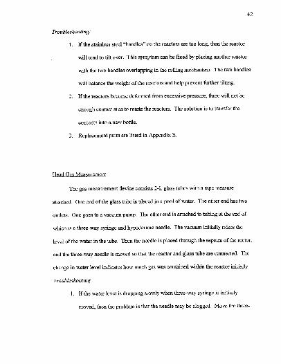
Troubleshooting:
l. If the stainless steel "handles" on the reactors are too long, then the reactor
will tend to tilt over. This symptom can be fixed by placing another reactor
with the two handles overlapping in the rolling mechanism. The two handles
will balance the weight of the reactors and help prevent further tilting.
2. If the reactors become deformed from excessive pressure, there will not be
enough contact area to rotate the reactors. The solution is to transfer the
contents into a new bottle.
3. Replacement parts are listed in Appendix E.
Head Gas Measurement
The gas measurement device consists 2-L glass tubes with a tape measure
attached. One end of the glass tube is placed in a pool of water. The other end has two
outlets. One goes to a vacuum pump. The other end is attached to tubing at the end of
which is a three-way syringe and hypodermic needle. The vacuum initially raises the
level of the water in the tube. Then the needle is placed through the septum of the rector,
and the three-way needle is moved so that the reactor and glass tube are connected. The
change in water level indicates how much gas was contained within the reactor initially.
Troubleshooti ng
l. If the water level is dropping slowly when three-way syringe is initially
moved, then the problem is that the needle may be clogged. Move the three-

43
way syringe to connect the syringe and needle. Try pulling air and/or water
through the needle into the syringe to remove any blockage.
2. If the water level will not remain constant when all openings are sealed, the
system is leaking. There are several places where leaks can occur. The glass
stopcock that controls the vacuum line may need additional vacuum grease.
Remove the stopcock and regrease. Also, the three-way syringe may leak if
particles are trapped between the rotating mechanism and housing. Try
washing the syringe with water, and if that fails, replace the syringe.
Countercurrent Procedures
The three reactors (labeled as shown in Figure 5) are removed &om the shaker and
allowed to reach ambient temperatures. Then, gas measurement values are taken for each
reactor. To prevent oxygen contamination, for all steps where the reactor is open, a
nitrogen purge is placed inside of the reactor.
The stopper and associated apparatus are removed, and a complete cap is placed
on each reactor. The reactors are then centrifuged for 10 minutes at 3500 rpm.
The liquid is then quantitatively removed from Reactor 1, and a liquid sample is
drawn for product characterization. The reactor with solids is then weighed. Solids are
quantitatively removed until the weight is 170 g, The following is then added: g g of
chicken manure, 12 g of gin trash, 2 g of CaCOn 0. 15 g of urea, and 40 ItL of CHIs. The
contents are mixed by hand, and the liquid from Reactor 2 is poured into Reactor 1. The
stopper is then replaced, and the reactor capped.

44
Reactor 2 is then weighed. Again solids are removed until the target weight is
reached. The target weight is 170 grams minus the mass of solids removed from reactor
1. Once the target mass has been reached, the solids removed Irom Reactor I are placed
in Reactor 2. Similar amounts of CaCOn urea, and CHI3 are added to Reactor 2. The
liquid from Reactor 3 is then poured into Reactor 2. The contents are mixed by hand, and
the reactor is sealed.
Reactor 3 undergoes a similar procedure as Reactor 2; however, the solids
removed from Reactor 3 are the product solids. These solids are collected and stored for
chamcterization. Also, because there is not another reactor from which to pour liquid into
reactor 3, 150 mL of fresh media is placed into Reactor 3.
Li uid Product Characterization
The product composition is determined with a Hewlett Packard 5890 Gas
Chromatograph. Also attached is a Hewlett Packard 7673A Controller/Automatic
Sampler to autoinject multiple samples. A Hewlett Packard 3396 Series Il Integrator
collects the output from the Gas Chromatograph for furthur analysis.
The complete procedure is listed in Appendix D of Loescher (1996).
Troubleshooting:
1. If the GC gives the error message for "Loop Down, " this message indicates
that the communications loop between the different components of the GC
setup is in error. One solution is to manually break the communication
connection by unplugging the small black wire from one of the components.

45
Then upon reconnection of the communications wire, the components will
automatically attempt to reconnect.

E. Equipment Parts
Apparatus
Description
Reactor
Bottle, 1000 mL
Supplier
Nalgene
Part Number
1000 mL PPCO
1/4" Stainless Steel Tubing RP Supply
Rolling Mechanism
Fan Motor
Bearings
AC Generators
Reducer Bushing
Set-screw coupling
Grainger 4M632
McMaster-Carr 7930K13
McMaster-Carr 6142K53
McMaster-Carr 6420K13
McMaster-Carr 6412K14
1/2" Stainless steel tubing RP Supply
Pully
Timing Belt
Motion Industries 16L050 X 1/2
Motion Industries 124L050

47
F. Supplier Information
Supplier
Bryan Livestock Commission
Company
Grainger
Address
6095 E State Highway 21
Bryan, TX 77808-8641
7777
Parnell
Houston, TX 77021
Phone Number
(409) 778-0904
(713) 748-8280
McMaster-Carr Supply Company P. O. Box 740100
Atlanta, GA 30374-0100
(404) 346-7000
Motion Industries, Inc. 1206 W. Wm. J. Bryan Parkway (409) 779-8485
Bryan TX 77803
R. P. Supply
Southwood Valley Turf
P. O. Box 19
Highway 21 East
Kurten, TX 77862
3312 Texas Ave S
College Station, TX 77845-0583
(409) 589-3113
(409) 696-6443