1.Introduction1.IntroductionThe standard cosmology is a successful framework for

interpreting observations. In spite of this fact there were certain questions which remained unsolved until 1980s.

For many years it was assumed that any solution of these problems would have to await a theory of quantum gravity.

The great success of cosmology in 1980s was the realization that an explanation of some of these puzzles might involve physics at lower energies: “only” 1015 Gev, vs 1019 Gev of quantum gravity.

THE CONCEPT OF INFLATION WAS BORN.

What follows is an outline of the main features of inflation in his “classical” form;

The reader will find more than one model of inflation in scientific literature; here we will refer to the standard inflation which involves a first order cosmological phase transition.

2.Classical problems of standard 2.Classical problems of standard isotropic cosmologyisotropic cosmology

2.1 The horizon problemFrom CBR observations we know that:

510T

TOn angular scales >> 1°.

Sandard cosmology contains a particle horizon of radius:

*

0

*2)(

*)(*

t

po tdtta

tatR In the radiation dominated era,when a(t) ~t 1/2. (We will use natural

units, c=1).

In the matter dominated era (a(t) ~t 2/3) :

*

0

*3)(

*)(*

t

po tdtta

tatR

R po(t0)=3t0 ~6000 Mpc h-1

At t= tls (last scattering) Rpo(tls)=3tls

Because of the expansion of the universe the universe at last scattering is now:

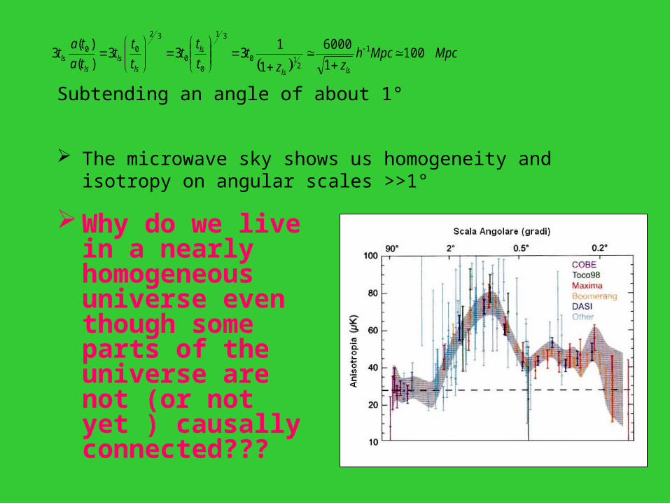
Subtending an angle of about 1°

The microwave sky shows us homogeneity and isotropy on angular scales >>1°

MpcMpch

zzt

t

tt

t

tt

ta

tat

lsls

ls

lsls

lsls 100

1

6000

1

1333

)(

)(3 1

210

31

00

32

00

Why do we live in a nearly homogeneous universe even though some parts of the universe are not (or not yet ) causally connected???

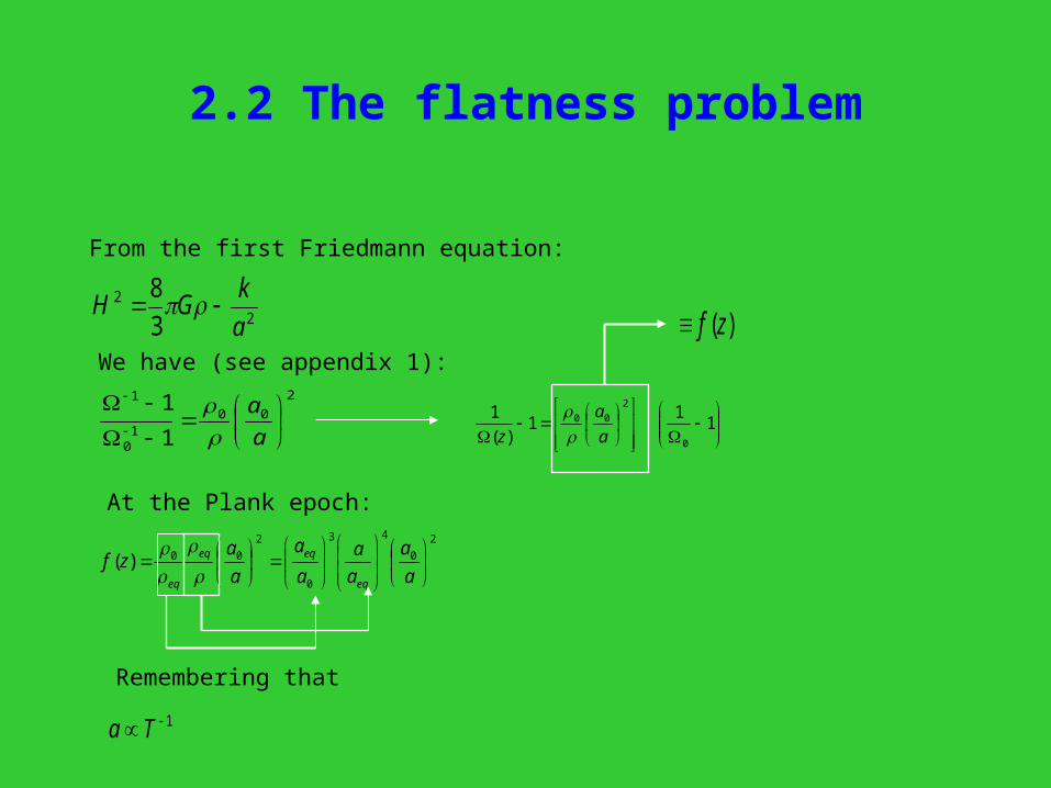
2.2 The flatness problem

From the first Friedmann equation:

22

3

8

a

kGH

We have (see appendix 1):2

001

0

1

1

1

a

a

1

11

)(

1

0

2

00

a

a

z

)(zf

At the Plank epoch:

2

0

43

0

2

00)(

a

a

a

a

a

a

a

azf

eq

eqeq

eq

Remembering that

1 Ta

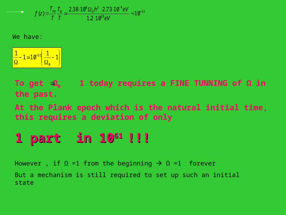
6128

4240 10

102.1

1073.21038.2)(

eV

eVh

T

T

T

Tzf beq

We have:

1

1101

1

0

61

To get Ω0 1 today requires a FINE TUNNING of Ω in the past.

At the Plank epoch which is the natural initial time, this requires a deviation of only

1 part in 101 part in 1061 61 !!!!!!

However , if Ω =1 from the beginning Ω =1 forever

But a mechanism is still required to set up such an initial state

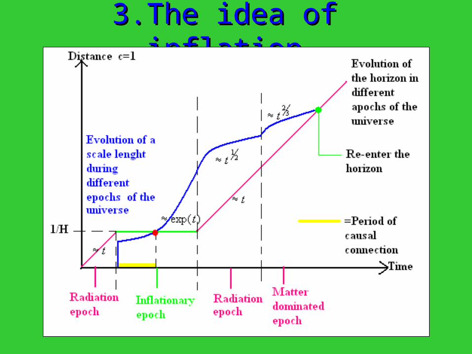
3.The idea of inflation3.The idea of inflation

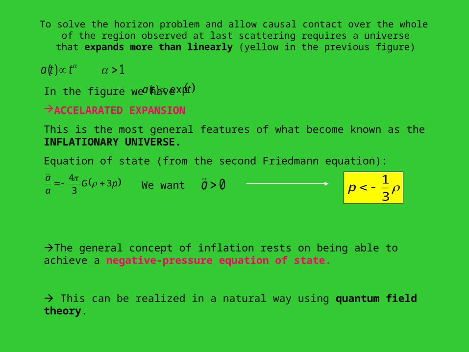
To solve the horizon problem and allow causal contact over the whole of the region observed at last scattering requires a universe that expands more than linearly (yellow in the previous figure)

1)( tta

In the figure we have

ACCELARATED EXPANSION

This is the most general features of what become known as the INFLATIONARY UNIVERSE.

Equation of state (from the second Friedmann equation):

tta exp)(

pGa

a3

3

4

We want 0a 3

1p

The general concept of inflation rests on being able to achieve a negative-pressure equation of state.

This can be realized in a natural way using quantum field theory.

4.Basic concepts of quantum 4.Basic concepts of quantum field theoryfield theory

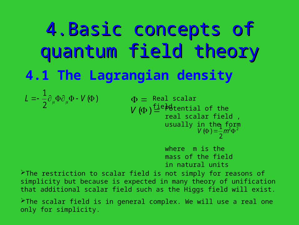
4.1 The Lagrangian density

)(2

1 VL Real scalar field

)(V Potential of the real scalar field , usually in the form

where m is the mass of the field in natural units

22

2

1)( mV

The restriction to scalar field is not simply for reasons of simplicity but because is expected in many theory of unification that additional scalar field such as the Higgs field will exist.

The scalar field is in general complex. We will use a real one only for simplicity.

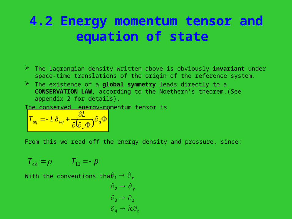
4.2 Energy momentum tensor and equation of state

The Lagrangian density written above is obviously invariant under space-time translations of the origin of the reference system.

The existence of a global symmetry leads directly to a CONSERVATION LAW, according to the Noethern’s theorem.(See appendix 2 for details).

The conserved energy-momentum tensor is

From this we read off the energy density and pressure, since:

With the conventions that

qqq

LLT

44T pT 11

t

z

y

x

ic

4

3

2

1

1

111

LLT

4

444

LLT

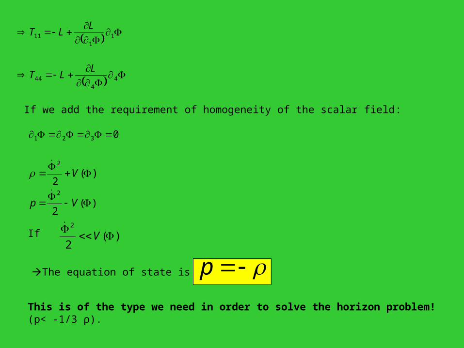
If we add the requirement of homogeneity of the scalar field:

0321

)(2

)(2

2

2

Vp

V

If )(2

2

V

The equation of state is : pThis is of the type we need in order to solve the horizon problem! (p< -1/3 ρ).

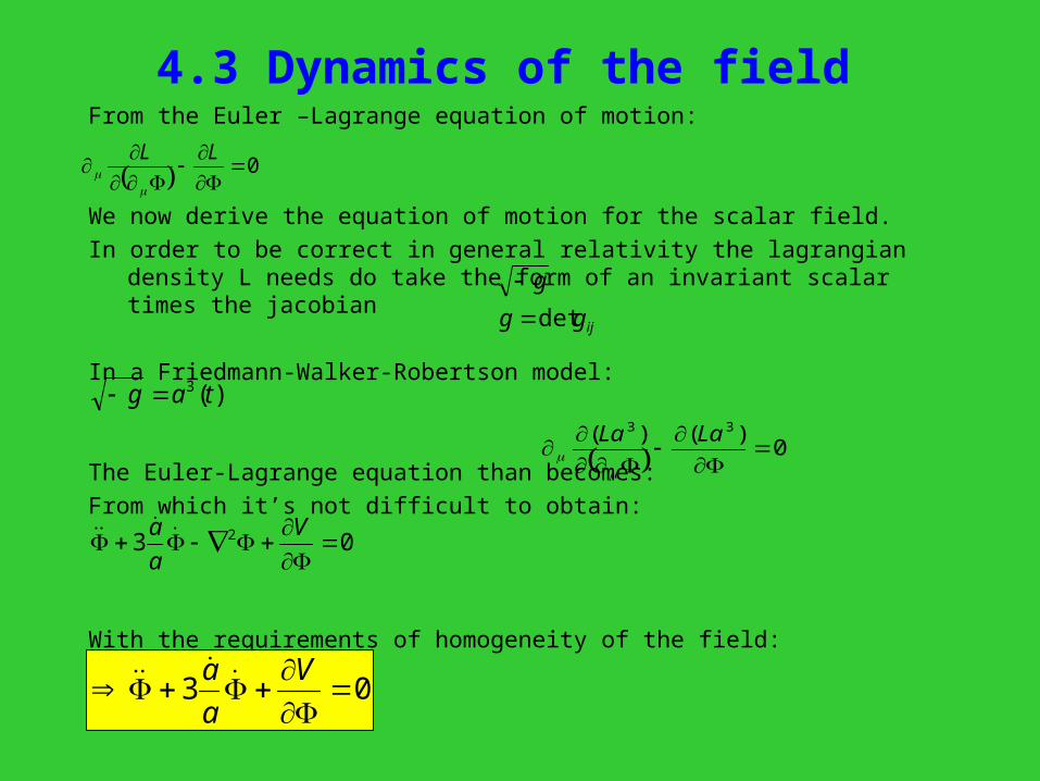
4.3 Dynamics of the fieldFrom the Euler –Lagrange equation of motion:

We now derive the equation of motion for the scalar field.

In order to be correct in general relativity the lagrangian density L needs do take the form of an invariant scalar times the jacobian

In a Friedmann-Walker-Robertson model:

The Euler-Lagrange equation than becomes:

From which it’s not difficult to obtain:

With the requirements of homogeneity of the field:

0

LL

ijgg

g

det

)(3 tag

0)()( 33

LaLa

03 2

V

a

a

03

V

a

a

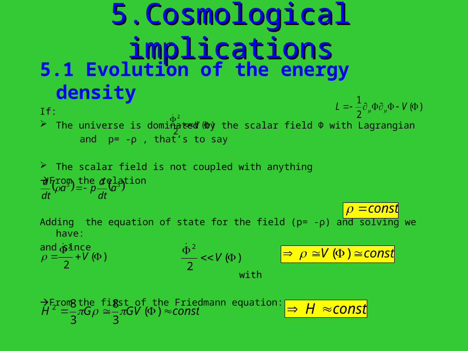
5.Cosmological implications5.Cosmological implications5.1 Evolution of the energy densityIf: The universe is dominated by the scalar field Φ with Lagrangian

and p= -ρ , that’s to say

The scalar field is not coupled with anything

From the relation

Adding the equation of state for the field (p= -ρ) and solving we have:

and since

with

From the first of the Friedmann equation:

)(2

1 VL

)(2

2

V

33 adt

dpa

dt

d

const

)(2

2

V

)(2

2

V constV )(

constGVGH )(3

8

3

82 constH

5.2 Exponential expansion

From the first Friedmann equation:

More then linear expansion: this is what we need in order to solve the horizon problem

constHa

a

2

2

aHa

Htea

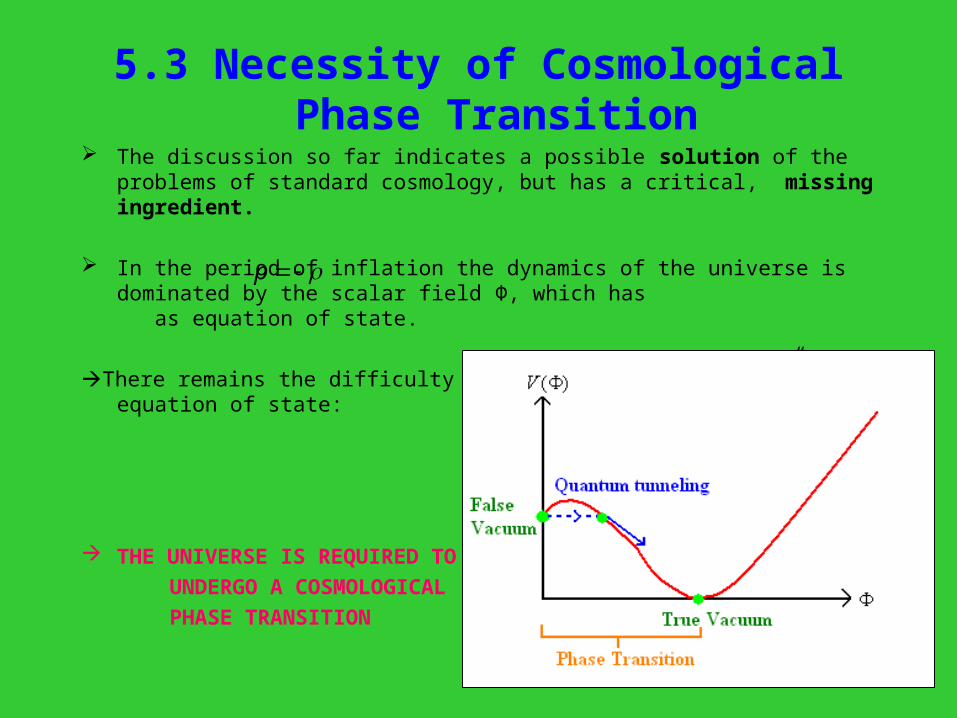
5.3 Necessity of Cosmological Phase Transition

The discussion so far indicates a possible solution of the problems of standard cosmology, but has a critical, missing ingredient.

In the period of inflation the dynamics of the universe is dominated by the scalar field Φ, which has as equation of state.

There remains the difficulty of returning to a “normal” equation of state:

THE UNIVERSE IS REQUIRED TO

UNDERGO A COSMOLOGICAL

PHASE TRANSITION

p

5.4 Necessity of Reheating

The exponential expansion produces a universe that is essentially devoid of normal matter and radiation;

Because of this the temperature of the universe becomes <<T, if T was the temperature at the beginning.

We know that at the end of the inflation the temperature has to be high enough in order to allow the violation of the barion number and nucleosynthesis.

A phase transition to a state of 0 vacuum energy, if istantaneous, would transfer the energy of the field to matter and radiation as latent heat.

THE UNIVERSE WOULD THEREFORE BE REHEATED

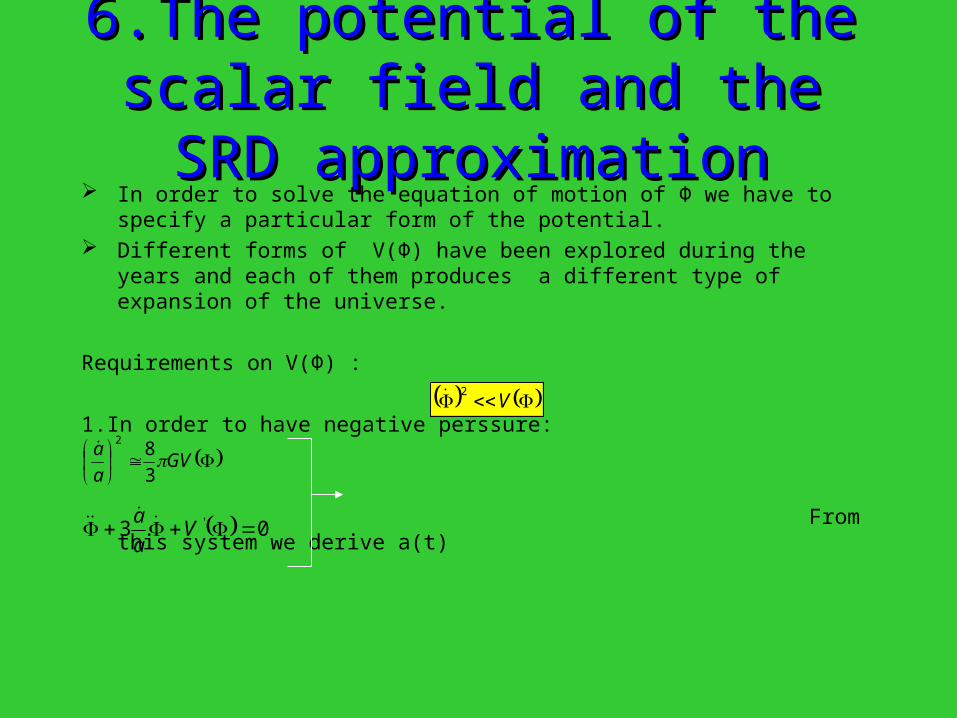
6.The potential of the scalar field 6.The potential of the scalar field and the SRD approximationand the SRD approximation

In order to solve the equation of motion of Φ we have to specify a particular form of the potential.

Different forms of V(Φ) have been explored during the years and each of them produces a different type of expansion of the universe.

Requirements on V(Φ) :

1.In order to have negative perssure:

From this system we derive a(t)

V2

GVa

a 3

82

03 ' Va

a

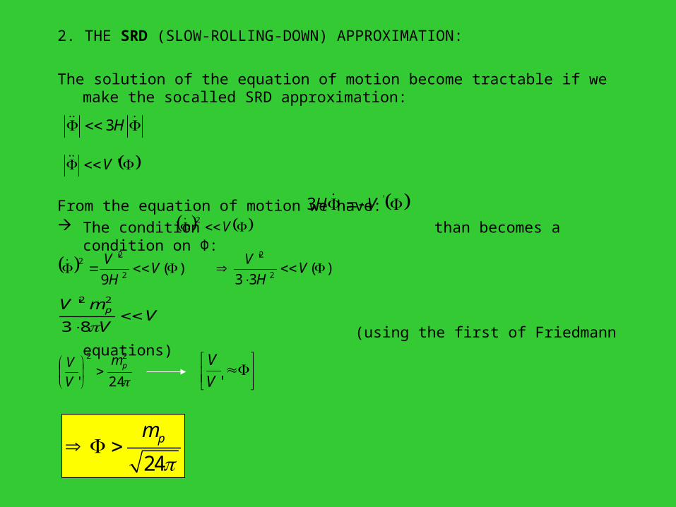
2. THE SRD (SLOW-ROLLING-DOWN) APPROXIMATION:

The solution of the equation of motion become tractable if we make the socalled SRD approximation:

From the equation of motion we have: The condition than becomes a condition on Φ:

(using the first of Friedmann equations)

H3

'V

'3 VH V

2

)(9

'2

22

VH

V )(33

'2

2

VH

V

VV

mV p 83

' 22

24'

22pm

V

V

'V

V

24pm

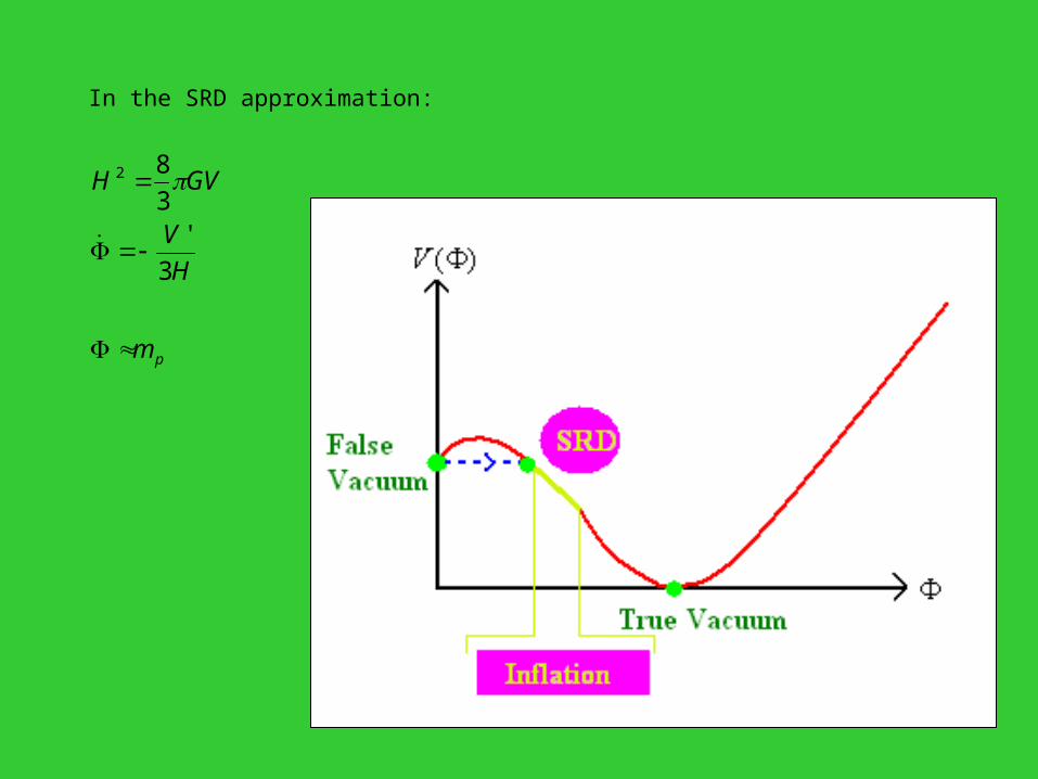
In the SRD approximation:

pm

H

V

GVH

3

'3

82

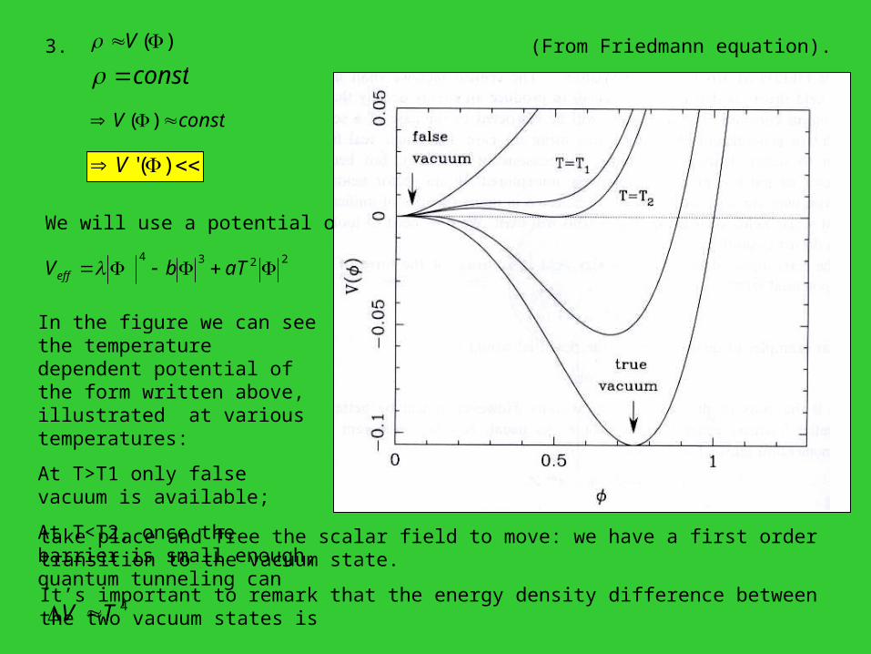
3. (From Friedmann equation).

We will use a potential of the form:

const)(V

constV )(

)('V

2234 aTbVeff

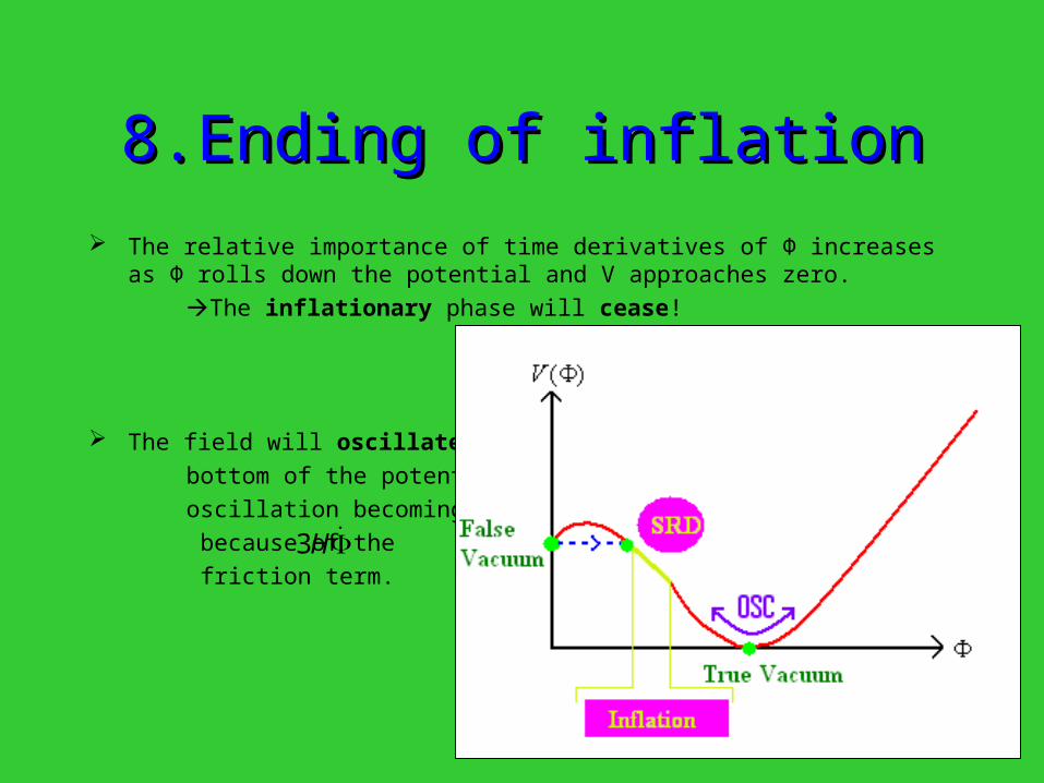
In the figure we can see the temperature dependent potential of the form written above, illustrated at various temperatures:

At T>T1 only false vacuum is available;

At T<T2, once the barrier is small enough, quantum tunneling can

take place and free the scalar field to move: we have a first order transition to the vacuum state.

It’s important to remark that the energy density difference between the two vacuum states is

4TV

7.The Inflation solution of 7.The Inflation solution of standard cosmology problemsstandard cosmology problems

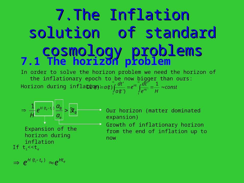
7.1 The horizon problemIn order to solve the horizon problem we need the horizon of the inflationary epoch to be

now bigger than ours:

Horizon during inflation: constHe

dte

ta

dttatOE

tHt

Ht

t

1'

)'(

')()(

'

Our horizon (matter dominated expansion)

Growth of inflationary horizon from the end of inflation up to nowExpansion of the horizon

during inflation

If ti<<te

00)( 3

1t

a

ae

H e

ttH ie

eei HtttH ee )(

Ha

ate eHte

003

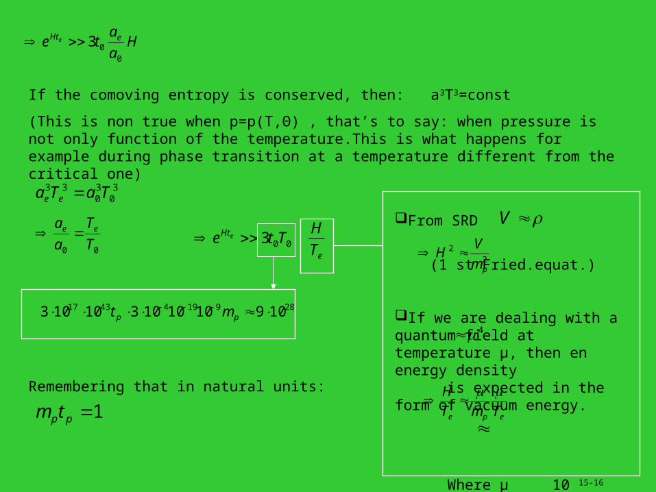
If the comoving entropy is conserved, then: a3T3=const

(This is non true when p=p(T,Θ) , that’s to say: when pressure is not only function of the temperature.This is what happens for example during phase transition at a temperature different from the critical one)

Remembering that in natural units:

30

30

33 TaTa ee

00 T

T

a

a ee e

Ht

T

HTte e

003

2891944317 109101010310103 pp mt

1pptm

From SRD

(1 st Fried.equat.)

If we are dealing with a quantum field at temperature μ, then en energy density is expected in the form of vacuum energy.

Where μ 10 15-16 Gev (From GUT theories

V

22

pm

VH

4

epe TmT

H

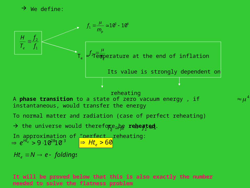
We define:

Te = Temperature at the end of inflation

Its value is strongly dependent on

reheating

1

2

f

f

T

H

e

431 1010

pmf

eTf

2

A phase transition to a state of zero vacuum energy , if instantaneous, would transfer the energy

To normal matter and radiation (case of perfect reheating)

the universe would therefore be reheated.

In approximation of “perfect” reheating:

It will be proved below that this is also exactly the number needed to solve the flatness problem

4

eT 12 f

32810109 eHte 60 eHt

foldingseNHte

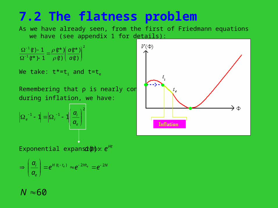
7.2 The flatness problemAs we have already seen, from the first of Friedmann equations we have (see appendix 1 for

details):

We take: t*=ti and t=te

Remembering that ρ is nearly constant

during inflation, we have:

2

1

1

)(

*)(

)(

*)(

1*)(

1)(

ta

ta

t

t

t

t

2

11 11

e

iie a

a

Exponential expansion: Hteta )(

NHtttH

e

i eeea

aeei 22)(

60N

Nie e 211 11

1e

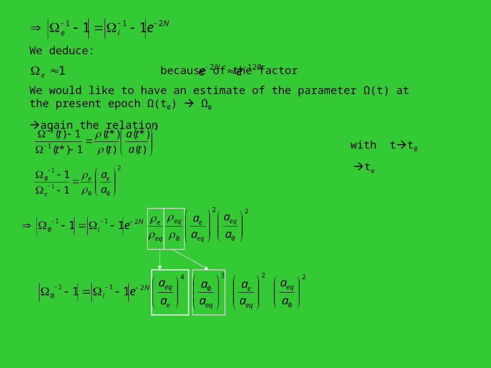
We deduce:

because of the factor

We would like to have an estimate of the parameter Ω(t) at the present epoch Ω(t0) Ω0

again the relation

with tt0

te

1202 ee N

2

1

1

)(

*)(

)(

*)(

1*)(

1)(

ta

ta

t

t

t

t

2

001

10

1

1

a

aee

e

2

0

2

0

2110 11

a

a

a

ae eq

eq

eeq

eq

eNi

2

0

23

0

4

2110 11

a

a

a

a

a

a

a

ae eq

eq

e

eqe

eqNi

eq

eNi

e

eqNi TT

Te

a

aae

0

221

2

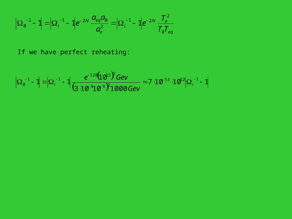
02110 111

110107

100010103

1011 15253

294

21512011

0

iiGev

Geve

If we have perfect reheating:

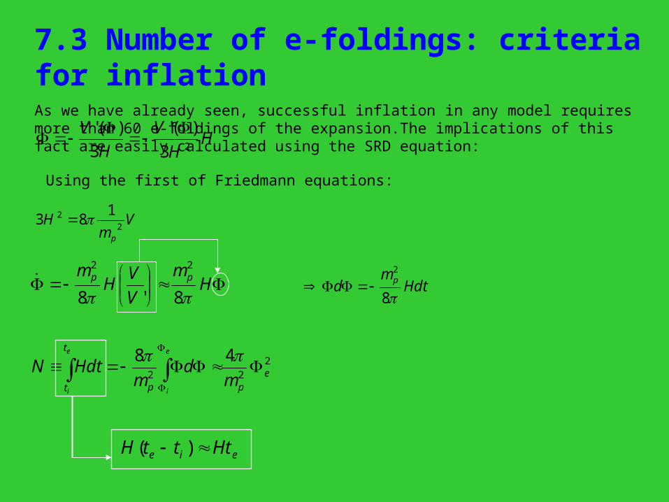
7.3 Number of e-foldings: criteria for inflationAs we have already seen, successful inflation in any model requires more than 60 e-foldings of the expansion.The implications of this fact are easily calculated using the SRD equation:

HH

V

H

V23

)('

3

)('

Vm

Hp

22 1

83

Using the first of Friedmann equations:

H

m

V

VH

m pp

8'8

22

Hdtm

d p

8

2

222

48e

p

t

t p md

mHdtN

e

i

e

i

eie HtttH )(

ppep

e mmHtm

24

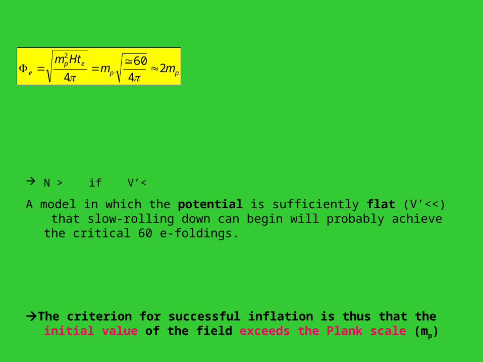
60

4

2

N > if V’<

A model in which the potential is sufficiently flat (V’<<) that slow-rolling down can begin will probably achieve the critical 60 e-foldings.

The criterion for successful inflation is thus that the initial value of the field exceeds the Plank scale (mp)

8.Ending of inflation8.Ending of inflation

The relative importance of time derivatives of Φ increases as Φ rolls down the potential and V approaches zero.

The inflationary phase will cease!

The field will oscillate about the

bottom of the potential, with

oscillation becoming damped

because of the

friction term.H3

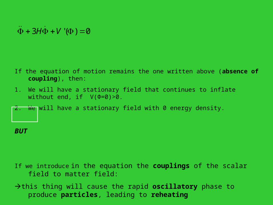
If the equation of motion remains the one written above (absence of coupling), then:

1. We will have a stationary field that continues to inflate without end, if V(Φ=0)>0.

2. We will have a stationary field with 0 energy density.

BUT

If we introduce in the equation the couplings of the scalar field to matter field:

this thing will cause the rapid oscillatory phase to produce particles, leading to reheating

0)('3 VH

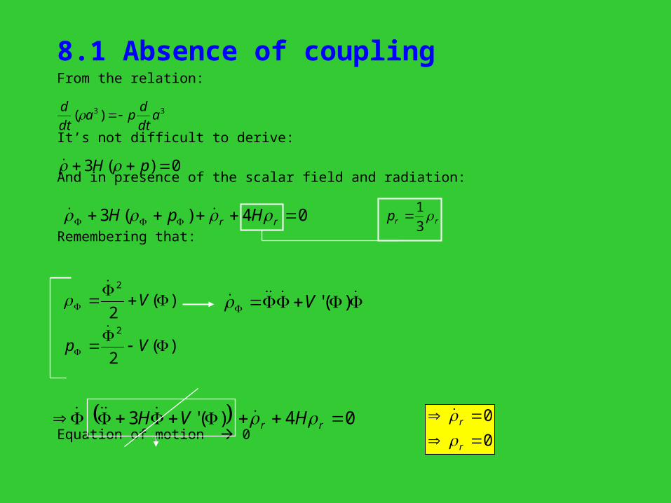
8.1 Absence of couplingFrom the relation:

It’s not difficult to derive:

And in presence of the scalar field and radiation:

Remembering that:

Equation of motion 0

33 )( adt

dpa

dt

d

0)(3 pH

04)(3 rr HpH rrp 3

1

)(2

)(2

2

2

Vp

V

)('V

0

0

r

r

04)('3 rr HVH

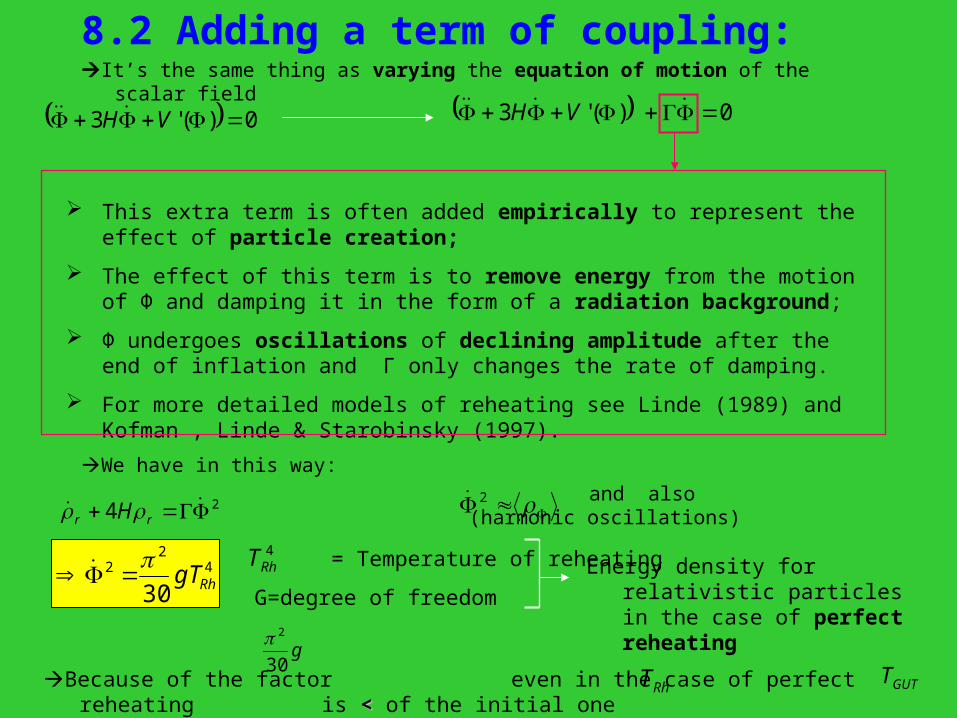
8.2 Adding a term of coupling:It’s the same thing as varying the equation of motion of the scalar field

We have in this way:

and also (harmonic oscillations)

0)('3 VH 0)('3 VH

This extra term is often added empirically to represent the effect of particle creation;

The effect of this term is to remove energy from the motion of Φ and damping it in the form of a radiation background;

Φ undergoes oscillations of declining amplitude after the end of inflation and Γ only changes the rate of damping.

For more detailed models of reheating see Linde (1989) and Kofman , Linde & Starobinsky (1997).

24 rr H 2

42

2

30 RhgT

= Temperature of reheating

G=degree of freedom

4RhT Energy density for relativistic

particles in the case of perfect reheating

Because of the factor even in the case of perfect reheating is << of the initial one

g30

2

RhT GUTT

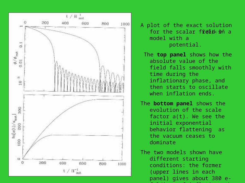
A plot of the exact solution for the scalar field in a model with a potential.

The top panel shows how the absolute value of the field falls smoothly with time during the inflationary phase, and then starts to oscillate when inflation ends.

The bottom panel shows the evolution of the scale factor a(t). We see the initial exponential behavior flattening as the vacuum ceases to dominate

The two models shown have different starting conditions: the former (upper lines in each panel) gives about 380 e-foldings of inflation; the latter only 150.

(From Peacock,1999).

2)( V

9. Relic fluctuations from Inflation9. Relic fluctuations from Inflation

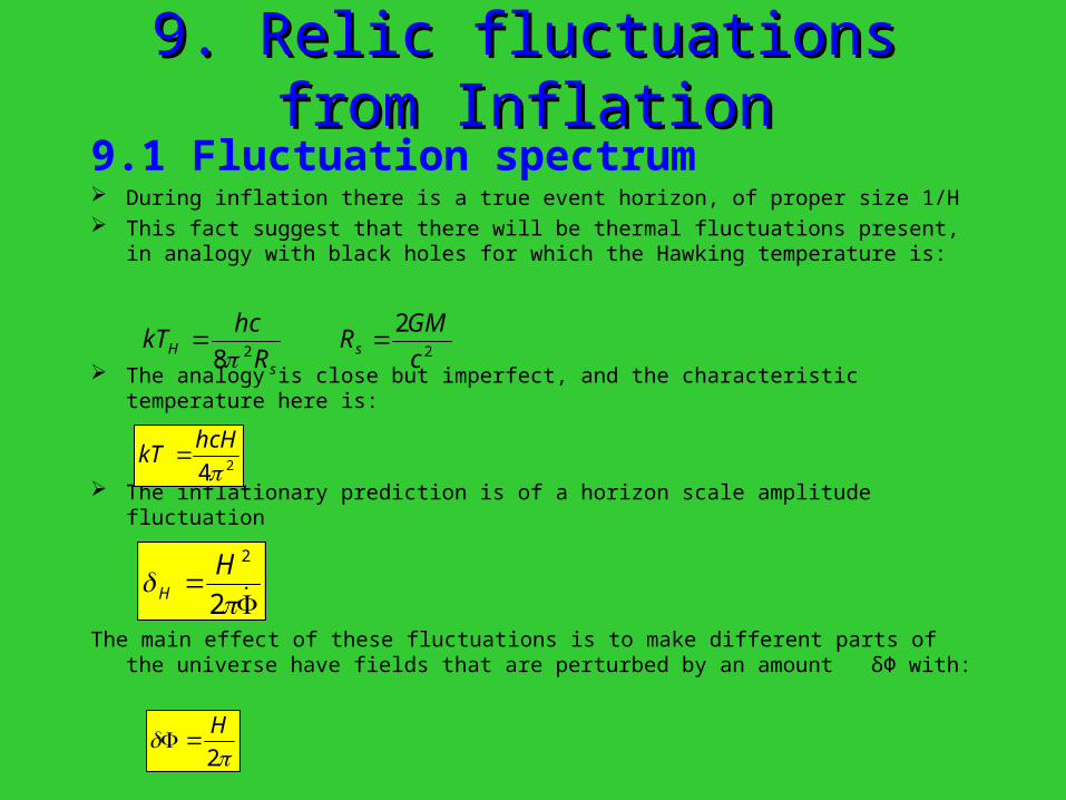
9.1 Fluctuation spectrum During inflation there is a true event horizon, of proper size 1/H This fact suggest that there will be thermal fluctuations present, in analogy with black

holes for which the Hawking temperature is:

The analogy is close but imperfect, and the characteristic temperature here is:

The inflationary prediction is of a horizon scale amplitude fluctuation

The main effect of these fluctuations is to make different parts of the universe have fields that are perturbed by an amount δΦ with:

22

2

8 c

GMR

R

hckT s

sH

24hcH

kT

2

2HH

2

H

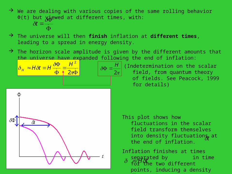
We are dealing with various copies of the same rolling behavior Φ(t) but viewed at different times, with:

The universe will then finish inflation at different times, leading to a spread in energy density.

The horizon scale amplitude is given by the different amounts that the universe have expanded following the end of inflation:

t

2

2HHtHH

2

H (Indetermination on the scalar field, from

quantum theory of fields. See Peacock, 1999 for details)

This plot shows how fluctuations in the scalar field transform themselves into density fluctuations at the end of inflation.

Inflation finishes at times separated by in time for the two different points, inducing a density fluctuation

t

tH

9.2 Inflation couplingFrom the SRD equation, we know that the number of e-foldings of inflation is:

If

Since N ≈ 60 and the observed value of fluctuations

(Really weak coupling!!!)

'3 2

V

dH

dHHdtN

4V

2

2

H

N

2321

3

332

'

3N

H

V

HHH

510 H

1510

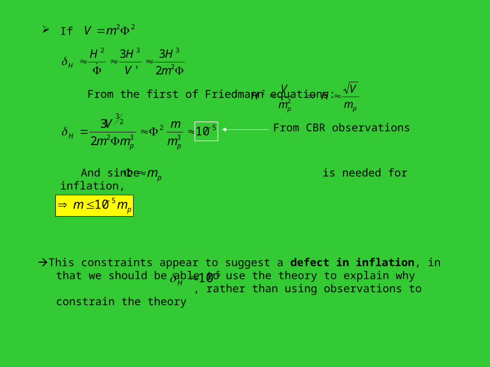
If

From the first of Friedmann equations:

And since is needed for inflation,

22mV

2

332

2

3

'

3

m

H

V

HHH

pp m

VH

m

VH

22

53

232

23

102

3

pp

H m

m

mm

V From CBR observations

pm

pmm 510

This constraints appear to suggest a defect in inflation, in that we should be able to use the theory to explain why , rather than using observations to constrain the theory510 H

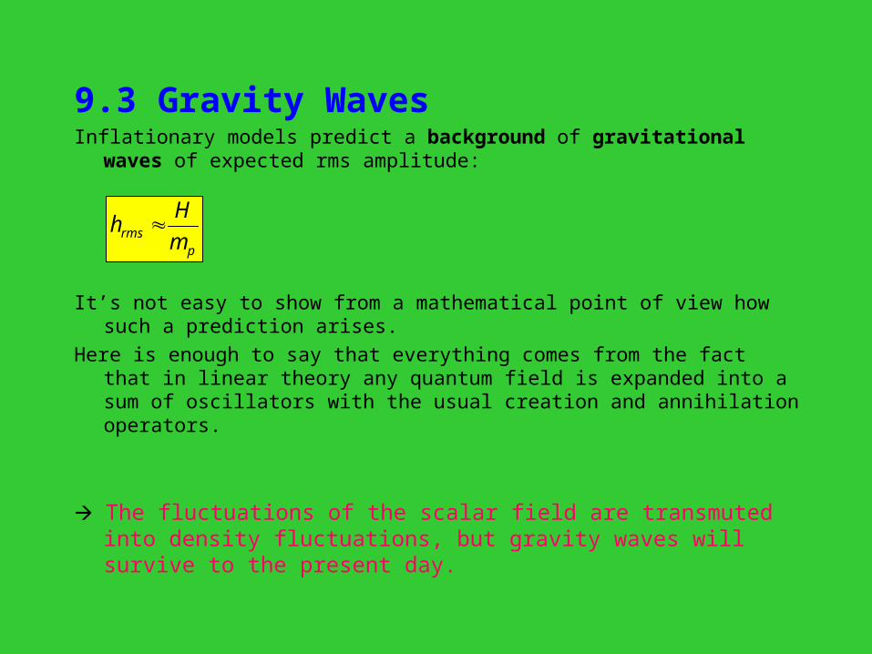
9.3 Gravity WavesInflationary models predict a background of gravitational waves of expected

rms amplitude:

It’s not easy to show from a mathematical point of view how such a prediction arises.

Here is enough to say that everything comes from the fact that in linear theory any quantum field is expanded into a sum of oscillators with the usual creation and annihilation operators.

The fluctuations of the scalar field are transmuted into density fluctuations, but gravity waves will survive to the present day.

prms m

Hh

10. Conclusion10. Conclusion

To summarize, inflation: Is able to give a satisfactory explanation to the

horizon and flatness problem; Is able to predict a scale invariant spectrum, but

problems arises with the amplitude of the fluctuations predicted (or alternatively with the coupling constant λ );

Is strongly linked with quantum field theory.

11.References11.References

• Kofman, Linde, Starobinsky,1997:hep-ph/9704452 • Linde,1989:Inflation and quantum cosmology,

Academic Press.• Lucchin,1990:Introduzione alla cosmologia, Zanichelli.• Peacock,1999:Cosmological physics, Cambridge

University Press.• Ramond:Quantum field theory.• Weinberg,1972:Gravitation and cosmology, John Wiley

and sons.

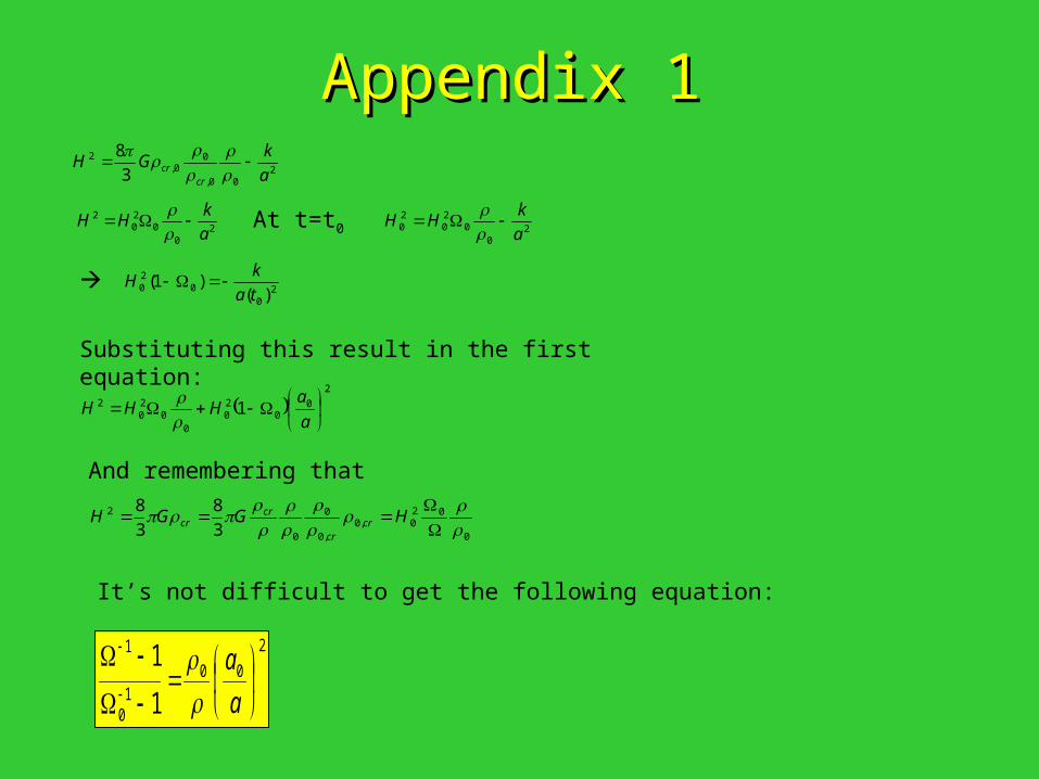
Appendix 1Appendix 12

00,

00,

2

3

8

a

kGH

crcr

20

020

2

a

kHH

20

020

20 a

kHH

At t=t0

20

020 )(

)1(ta

kH

Substituting this result in the first equation:

2

00

20

00

20

2 1

a

aHHH

And remembering that

0

020,0

,0

0

0

2

3

8

3

8

HGGH crcr

crcr

It’s not difficult to get the following equation:

2

001

0

1

1

1

a

a

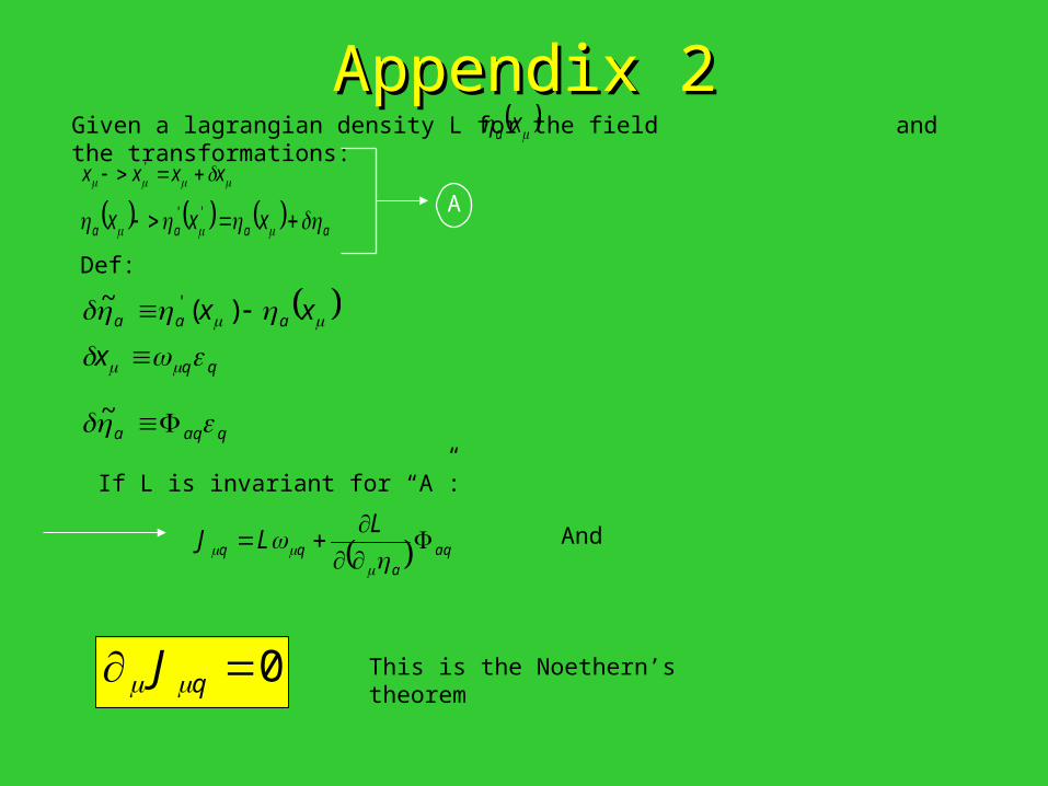
Appendix 2Appendix 2Given a lagrangian density L for the field and the transformations: xa

xxxx '

Def:

aaaa xxx ''

qaqa

qq

aaa

x

xx

~

)(~ '

A

If L is invariant for “A”:

aqa

qq

LLJ

And

0 qJ This is the Noethern’s theorem

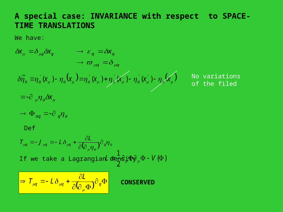
A special case: INVARIANCE with respect to SPACE-TIME TRANSLATIONS

We have:

qq xx

qq

qq x

xxxxxx aaaaaaa )()()()(~ '''''' No variations of the filed

xa

aqaq

Def

aqa

qqq

LLJT

If we take a Lagrangian density )(2

1 VL

qqq

LLT

CONSERVED