1introduction - wiley

1

CHAPTER OPENING PHOTO: The nature of air bubbles rising in a liquid is a function of fluid properties such as density, viscosity, and surface tension. (Left: air in oil; right: air in soap.)(Photographs copyright 2007 by Andrew Davidhazy, Rochester Institute of Technology.)

1Introduction

Learning Objectives

After completing this chapter, you should be able to:

■ determine the dimensions and units of physical quantities.

■ identify the key fluid properties used in the analysis of fluid behavior.

■ calculate common fluid properties given appropriate information.

■ explain effects of fluid compressibility.

■ use the concepts of viscosity, vapor pressure, and surface tension.

Fluid mechanics is the discipline within the broad field of applied mechanics that is concerned

with the behavior of liquids and gases at rest or in motion. It covers a vast array of phenomena

that occur in nature (with or without human intervention), in biology, and in numerous engineered,

invented, or manufactured situations. There are few aspects of our lives that do not involve flu-

ids, either directly or indirectly.

The immense range of different flow conditions is mind-boggling and strongly dependent

on the value of the numerous parameters that describe fluid flow. Among the long list of para-

meters involved are (1) the physical size of the flow, ; (2) the speed of the flow, V; and (3) the

pressure, p, as indicated in the figure in the margin for a light aircraft parachute recovery sys-

tem. These are just three of the important parameters that, along with many others, are dis-

cussed in detail in various sections of this book. To get an inkling of the range of some of the

parameter values involved and the flow situations generated, consider the following.

Size,

Every flow has a characteristic (or typical) length associated with it. For example, for

flow of fluid within pipes, the pipe diameter is a characteristic length. Pipe flows include

/

/

�

p

V

(Photograph courtesy of CIRRUS Design Corporation.)

c01Introduction.qxd 9/21/12 3:41 PM

COPYRIG

HTED M

ATERIAL

2 Chapter 1 ■ Introduction

the flow of water in the pipes in our homes, the blood flow in our arteries and veins,

and the airflow in our bronchial tree. They also involve pipe sizes that are not within

our everyday experiences. Such examples include the flow of oil across Alaska through

a 1.2 meter diameter, 1286 km long pipe and, at the other end of the size scale, the new

area of interest involving flow in nano scale pipes whose diameters are on the order of

10�8 m. Each of these pipe flows has important characteristics that are not found in the

others.

Characteristic lengths of some other flows are shown in Fig. 1.1a.

Speed, VAs we note from The Weather Channel, on a given day the wind speed may cover what

we think of as a wide range, from a gentle 8 km/h breeze to a 160 km/h hurricane or a

400 km/h tornado. However, this speed range is small compared to that of the almost

imperceptible flow of the fluid-like magma below the Earth’s surface that drives the con-

tinental drift motion of the tectonic plates at a speed of about 2 � 10�8 m/s or the hyper-

sonic airflow past a meteor as it streaks through the atmosphere at 3 � 104 m/s.

Characteristic speeds of some other flows are shown in Fig. 1.1b.

Pressure, pThe pressure within fluids covers an extremely wide range of values. We are accustomed

to the 241 kPa pressure within our car’s tires, the “120 over 70” typical blood pressure read-

ing, or the standard 101.3 kPa atmospheric pressure. However, the large 690 MPa pressure

in the hydraulic ram of an earth mover or the tiny 14 � 10�6 kPa pressure of a sound wave

generated at ordinary talking levels are not easy to comprehend.

Characteristic pressures of some other flows are shown in Fig. 1.1c.

104

106

108

Jupiter red spot diameter

Ocean current diameter

Diameter of hurricane

Mt. St. Helens plume

Average width of middleMississippi River

Boeing 787NACA Ames wind tunnel

Diameter of Space Shuttlemain engine exhaust jet

Outboard motor prop

Water pipe diameter

Raindrop

Water jet cutter widthAmoebaThickness of lubricating oillayer in journal bearingDiameter of smallest bloodvessel

Artificial kidney filterpore size

Nano scale devices

102

100

10-4

10-2

10-6

10-8

�, m

104

106

Meteor entering atmosphere

Space Shuttle reentry

Rocket nozzle exhaustSpeed of sound in airTornado

Water from fire hose nozzleFlow past bike rider

Mississippi River

Syrup on pancake

Microscopic swimminganimal

Glacier flow

Continental drift

102

100

10 4

10-2

10-6

10-8

V, m

/s

104

106

Sound pressure at normaltalking

102

100

10-4

10-2

10-6

p, k

Pa

(10

3 ×

N/m

2)

Vacuum pump

Car engine combustion

Scuba tankHydraulic ram

Mariana Trench in PacificOcean

Waterjet cutting

Pressure at 64 km altitude

Pressure change causingears to "pop" in elevator

Atmospheric pressure onMars

Standard atmosphere

Fire hydrantAuto tire

"Excess pressure" on handheld out of car traveling96 km/hr

(a) (b) (c)

■ Figure 1.1 Characteristic values of some fluid flow parameters for a variety of flows: (a) object size,(b) fluid speed, (c) fluid pressure.

V1.1 Mt. St. Helenseruption

V1.2 E. coli swim-ming


The list of fluid mechanics applications goes on and on. But you get the point. Fluid me-

chanics is a very important, practical subject that encompasses a wide variety of situations. It is

very likely that during your career as an engineer you will be involved in the analysis and de-

sign of systems that require a good understanding of fluid mechanics. Although it is not possi-

ble to adequately cover all of the important areas of fluid mechanics within one book, it is hoped

that this introductory text will provide a sound foundation of the fundamental aspects of fluid

mechanics.

1.1 Some Characteristics of Fluids

1.1 Some Characteristics of Fluids 3

One of the first questions we need to explore is––what is a fluid? Or we might ask–what is

the difference between a solid and a fluid? We have a general, vague idea of the difference.

A solid is “hard” and not easily deformed, whereas a fluid is “soft” and is easily deformed

1we can readily move through air2. Although quite descriptive, these casual observations of the

differences between solids and fluids are not very satisfactory from a scientific or engineer-

ing point of view. A closer look at the molecular structure of materials reveals that matter that

we commonly think of as a solid 1steel, concrete, etc.2 has densely spaced molecules with large

intermolecular cohesive forces that allow the solid to maintain its shape, and to not be easily

deformed. However, for matter that we normally think of as a liquid 1water, oil, etc.2, the mol-

ecules are spaced farther apart, the intermolecular forces are smaller than for solids, and the

molecules have more freedom of movement. Thus, liquids can be easily deformed 1but not eas-

ily compressed2 and can be poured into containers or forced through a tube. Gases 1air, oxygen,

etc.2 have even greater molecular spacing and freedom of motion with negligible cohesive in-

termolecular forces, and as a consequence are easily deformed 1and compressed2 and will com-

pletely fill the volume of any container in which they are placed. Both liquids and gases are

fluids.

Although the differences between solids and fluids can be explained qualitatively on the

basis of molecular structure, a more specific distinction is based on how they deform under the

action of an external load. Specifically, a fluid is defined as a substance that deforms continu-ously when acted on by a shearing stress of any magnitude. A shearing stress 1force per unit

area2 is created whenever a tangential force acts on a surface as shown by the figure in the mar-

gin. When common solids such as steel or other metals are acted on by a shearing stress, they

will initially deform 1usually a very small deformation2, but they will not continuously deform

1flow2. However, common fluids such as water, oil, and air satisfy the definition of a fluid—that

is, they will flow when acted on by a shearing stress. Some materials, such as slurries, tar, putty,

toothpaste, and so on, are not easily classified since they will behave as a solid if the applied

shearing stress is small, but if the stress exceeds some critical value, the substance will flow.

The study of such materials is called rheology and does not fall within the province of classical

fluid mechanics. Thus, all the fluids we will be concerned with in this text will conform to the

definition of a fluid given previously.

F l u i d s i n t h e N e w s

Will what works in air work in water? For the past few years a

San Francisco company has been working on small, maneuver-

able submarines designed to travel through water using wings,

controls, and thrusters that are similar to those on jet airplanes.

After all, water (for submarines) and air (for airplanes) are both flu-

ids, so it is expected that many of the principles governing the flight

of airplanes should carry over to the “flight” of winged submarines.

Of course, there are differences. For example, the submarine must

be designed to withstand external pressures of nearly 4826 kPa

greater than that inside the vehicle. On the other hand, at high

altitude where commercial jets fly, the exterior pressure is 24 kPa

rather than standard sea-level pressure of 101.3 kPa, so the vehi-

cle must be pressurized internally for passenger comfort. In both

cases, however, the design of the craft for minimal drag, maxi-

mum lift, and efficient thrust is governed by the same fluid dy-

namic concepts.

Both liquids andgases are fluids.

F

Surface


Although the molecular structure of fluids is important in distinguishing one fluid from an-

other, it is not yet practical to study the behavior of individual molecules when trying to describe

the behavior of fluids at rest or in motion. Rather, we characterize the behavior by considering

the average, or macroscopic, value of the quantity of interest, where the average is evaluated over

a small volume containing a large number of molecules. Thus, when we say that the velocity at

a certain point in a fluid is so much, we are really indicating the average velocity of the mole-

cules in a small volume surrounding the point. The volume is small compared with the physical

dimensions of the system of interest, but large compared with the average distance between mol-

ecules. Is this a reasonable way to describe the behavior of a fluid? The answer is generally yes,

since the spacing between molecules is typically very small. For gases at normal pressures and

temperatures, the spacing is on the order of and for liquids it is on the order of

The number of molecules per cubic millimeter is on the order of for gases and for liq-

uids. It is thus clear that the number of molecules in a very tiny volume is huge and the idea of

using average values taken over this volume is certainly reasonable. We thus assume that all the

fluid characteristics we are interested in 1pressure, velocity, etc.2 vary continuously throughout

the fluid—that is, we treat the fluid as a continuum. This concept will certainly be valid for all

the circumstances considered in this text. One area of fluid mechanics for which the continuum

concept breaks down is in the study of rarefied gases such as would be encountered at very high

altitudes. In this case the spacing between air molecules can become large and the continuum

concept is no longer acceptable.

10211018

10�7 mm.10�6 mm,


1.2 Dimensions, Dimensional Homogeneity, and Units

Since in our study of fluid mechanics we will be dealing with a variety of fluid characteristics,

it is necessary to develop a system for describing these characteristics both qualitatively and

quantitatively. The qualitative aspect serves to identify the nature, or type, of the characteristics 1such

as length, time, stress, and velocity2, whereas the quantitative aspect provides a numerical measure

of the characteristics. The quantitative description requires both a number and a standard by which

various quantities can be compared. The standard for length is a meter, for time an hour or second,

and for mass, a kilogram. Such standards are called units, and several systems of units are in com-

mon use as described in the following section. The qualitative description is conveniently given in

terms of certain primary quantities, such as length, L, time, T, mass, M, and temperature, These

primary quantities can then be used to provide a qualitative description of any other secondary quan-tity: for example, and so on, where the symbol is

used to indicate the dimensions of the secondary quantity in terms of the primary quantities. Thus,

to describe qualitatively a velocity, V, we would write

and say that “the dimensions of a velocity equal length divided by time.” The primary quantities

are also referred to as basic dimensions.For a wide variety of problems involving fluid mechanics, only the three basic dimensions, L,

T, and M are required. Alternatively, L, T, and F could be used, where F is the basic dimensions of

force. Since Newton’s law states that force is equal to mass times acceleration, it follows that

or Thus, secondary quantities expressed in terms of M can be expressed

in terms of F through the relationship above. For example, stress, is a force per unit area, so that

but an equivalent dimensional equation is Table 1.1 provides a list of di-

mensions for a number of common physical quantities.

All theoretically derived equations are dimensionally homogeneous—that is, the dimensions of

the left side of the equation must be the same as those on the right side, and all additive separate terms

must have the same dimensions. We accept as a fundamental premise that all equations describing phys-

ical phenomena must be dimensionally homogeneous. If this were not true, we would be attempting to

equate or add unlike physical quantities, which would not make sense. For example, the equation for

the velocity, V, of a uniformly accelerated body is

(1.1)V � V0 � at

s � ML�1T �2.s � FL�2,

s,

M � FL�1 T 2.F � MLT

�2

V � LT �1

�density � ML�3,velocity � LT �1,area � L2,

™.

Fluid characteris-tics can be de-scribed qualitativelyin terms of certainbasic quantitiessuch as length,time, and mass.


1.2 Dimensions, Dimensional Homogeneity, and Units 5

where is the initial velocity, a the acceleration, and t the time interval. In terms of dimensions

the equation is

and thus Eq. 1.1 is dimensionally homogeneous.

Some equations that are known to be valid contain constants having dimensions. The equa-

tion for the distance, d, traveled by a freely falling body can be written as

(1.2)

and a check of the dimensions reveals that the constant must have the dimensions of if the

equation is to be dimensionally homogeneous. Actually, Eq. 1.2 is a special form of the well-known

equation from physics for freely falling bodies,

(1.3)

in which g is the acceleration of gravity. Equation 1.3 is dimensionally homogeneous and valid in

any system of units. For the equation reduces to Eq. 1.2 and thus Eq. 1.2 is valid

only for the system of units using meter and seconds. Equations that are restricted to a particular

system of units can be denoted as restricted homogeneous equations, as opposed to equations valid

in any system of units, which are general homogeneous equations. The preceding discussion indi-

cates one rather elementary, but important, use of the concept of dimensions: the determination of

one aspect of the generality of a given equation simply based on a consideration of the dimensions

of the various terms in the equation. The concept of dimensions also forms the basis for the pow-

erful tool of dimensional analysis, which is considered in detail in Chapter 7.

Note to the users of this text. All of the examples in the text use a consistent problem-

solving methodology, which is similar to that in other engineering courses such as statics. Each

example highlights the key elements of analysis: Given, Find, Solution, and Comment.The Given and Find are steps that ensure the user understands what is being asked in the

problem and explicitly list the items provided to help solve the problem.

The Solution step is where the equations needed to solve the problem are formulated and

the problem is actually solved. In this step, there are typically several other tasks that help to set

g � 9.81 m�s2

d �gt

2

2

LT �2

d � 16.1t 2

LT �1 � LT �1 � LT �2T

V0

Table 1.1

Dimensions Associated with Common Physical Quantities

FLT MLTSystem System

Acceleration

Angle

Angular acceleration

Angular velocity

Area

Density

Energy FLForce FFrequency

Heat FL

Length L LMass MModulus of elasticity

Moment of a force FLMoment of inertia 1area2

Moment of inertia 1mass2

Momentum FT MLT �1

ML2FLT 2

L4L4

ML2T �2

ML�1T �2FL�2

FL�1T 2

ML2T �2

T �1T �1

MLT �2

ML2T �2

ML�3FL�4T 2

L2L2

T �1T �1

T �2T �2

M 0L0T 0F 0L0T 0LT �2LT �2

General homoge-neous equationsare valid in anysystem of units.

FLT MLTSystem System

Power

Pressure

Specific heat

Specific weight

Strain

Stress

Surface tension

Temperature

Time T T

Torque FL

Velocity

Viscosity 1dynamic2

Viscosity 1kinematic2

Volume

Work FL ML2T�2

L3L3

L2T �1L2T �1

ML�1T �1FL�2T

LT �1LT �1

ML2T �2

™™MT �2FL�1

ML�1T �2FL�2

M 0L0T 0F 0L0T 0ML�2T �2FL�3

L2T �2™�1L2T �2™�1

ML�1T �2FL�2

ML2T �3FLT �1



up the solution and are required to solve the problem. The first is a drawing of the problem; where

appropriate, it is always helpful to draw a sketch of the problem. Here the relevant geometry and

coordinate system to be used as well as features such as control volumes, forces and pressures,

velocities, and mass flow rates are included. This helps in gaining a visual understanding of the

problem. Making appropriate assumptions to solve the problem is the second task. In a realistic

engineering problem-solving environment, the necessary assumptions are developed as an integral

part of the solution process. Assumptions can provide appropriate simplifications or offer useful

constraints, both of which can help in solving the problem. Throughout the examples in this text,

the necessary assumptions are embedded within the Solution step, as they are in solving a real-

world problem. This provides a realistic problem-solving experience.

The final element in the methodology is the Comment. For the examples in the text, this

section is used to provide further insight into the problem or the solution. It can also be a point

in the analysis at which certain questions are posed. For example: Is the answer reasonable,

and does it make physical sense? Are the final units correct? If a certain parameter were

changed, how would the answer change? Adopting this type of methodology will aid

in the development of problem-solving skills for fluid mechanics, as well as other engineering

disciplines.

GIVEN A liquid flows through an orifice located in the side of

a tank as shown in Fig. E1.1. A commonly used equation for de-

termining the volume rate of flow, Q, through the orifice is

where A is the area of the orifice, g is the acceleration of gravity,

and h is the height of the liquid above the orifice.

FIND Investigate the dimensional homogeneity of this formula.

Q � 0.61 A12gh

SOLUTION

Restricted and General Homogeneous Equations

and, therefore, the equation expressed as Eq. 1 can only be

dimensionally correct if the number 2.70 has the dimensions of

Whenever a number appearing in an equation or

formula has dimensions, it means that the specific value of the

number will depend on the system of units used. Thus,

for the case being considered with meter and seconds used as

units, the number 2.70 has units of Equation 1 will only

give the correct value for when A is expressed in

square meter and h in meter. Thus, Eq. 1 is a restricted homo-

geneous equation, whereas the original equation is a generalhomogeneous equation that would be valid for any consistent

system of units.

COMMENT A quick check of the dimensions of the vari-

ous terms in an equation is a useful practice and will often be

helpful in eliminating errors—that is, as noted previously, all

physically meaningful equations must be dimensionally ho-

mogeneous. We have briefly alluded to units in this example,

and this important topic will be considered in more detail in

the next section.

Q 1in m3�s2m1� 2�s.

L1� 2T �1.

EXAMPLE 1.1

The dimensions of the various terms in the equation are Q � volume/time �

. L3T�1, A � area �. L2, g � acceleration of gravity �

.

LT�2, and .

These terms, when substituted into the equation, yield the dimen-

sional form:

or

It is clear from this result that the equation is dimensionally

homogeneous 1both sides of the formula have the same dimensions

of 2, and the number 0.61 is dimensionless.

If we were going to use this relationship repeatedly, we might

be tempted to simplify it by replacing g with its standard value of

and rewriting the formula as

(1)

A quick check of the dimensions reveals that

L3T �1 � 12.702 1L5� 22

Q � 2.70 A1h

9.81 m�s2

12L3T �1

1L3T �12 � 30.6112 4 1L3T �12

1L3T �12 � 10.612 1L22 112 2 1LT �221� 21L21� 2

h � height � L

(a)

Q

h

A

(b)

■ Figure E1.1


1.2.1 Systems of Units

In addition to the qualitative description of the various quantities of interest, it is generally neces-

sary to have a quantitative measure of any given quantity. For example, if we measure the width

of this page in the book and say that it is 10 units wide, the statement has no meaning until the

unit of length is defined. If we indicate that the unit of length is a meter, and define the meter as

some standard length, a unit system for length has been established 1and a numerical value can be

given to the page width2. In addition to length, a unit must be established for each of the remain-

ing basic quantities 1force, mass, time, and temperature2. There are several systems of units in use,

and we shall consider three systems that are commonly used in engineering.

International System (SI). In 1960 the Eleventh General Conference on Weights and

Measures, the international organization responsible for maintaining precise uniform standards of

measurements, formally adopted the International System of Units as the international standard.

This system, commonly termed SI, has been widely adopted worldwide and is widely used 1although

certainly not exclusively2 in the United States. It is expected that the long-term trend will be for all

countries to accept SI as the accepted standard and it is imperative that engineering students become

familiar with this system. In SI the unit of length is the meter 1m2, the time unit is the second 1s2,the mass unit is the kilogram 1kg2, and the temperature unit is the kelvin 1K2. Note that there is no

degree symbol used when expressing a temperature in kelvin units. The kelvin temperature scale

is an absolute scale and is related to the Celsius 1centigrade2 scale through the relationship

Although the Celsius scale is not in itself part of SI, it is common practice to specify temperatures

in degrees Celsius when using SI units.

The force unit, called the newton 1N2, is defined from Newton’s second law as

Thus, a 1 N force acting on a 1 kg mass will give the mass an acceleration of 1 Standard grav-

ity in SI is 1commonly approximated as 2 so that a 1 kg mass weighs 9.81 N un-

der standard gravity. Note that weight and mass are different, both qualitatively and quantitatively! The

unit of work in SI is the joule 1J2, which is the work done when the point of application of a 1 N force

is displaced through a 1 m distance in the direction of a force. Thus,

The unit of power is the watt 1W2 defined as a joule per second. Thus,

Prefixes for forming multiples and fractions of SI units are given in Table 1.2. For example,

the notation kN would be read as “kilonewtons” and stands for Similarly, mm would be

read as “millimeters” and stands for The centimeter is not an accepted unit of length in

the SI system, so for most problems in fluid mechanics in which SI units are used, lengths will be

expressed in millimeters or meters.

10�3 m.

103 N.

1 W � 1 J�s � 1 N # m�s

1 J � 1 N # m

9.81 m�s29.807 m�s2

m�s2.

1 N � 11 kg2 11 m �s22

K � °C � 273.15

1°C2

1.2 Dimensions, Dimensional Homogeneity, and Units 7

In mechanics it isvery important todistinguish betweenweight and mass.

Table 1.2

Prefixes for SI Units

Factor by Which UnitIs Multiplied Prefix Symbol

peta P

tera T

giga G

mega M

kilo k

hecto h

10 deka da

deci d10�1

102

103

106

109

1012

1015

Factor by Which UnitIs Multiplied Prefix Symbol

centi c

milli m

micro

nano n

pico p

femto f

atto a10�18

10�15

10�12

10�9

m10�6

10�3

10�2


SI UnitsEXAMPLE 1.2

GIVEN A tank of liquid having a total mass of 36 kg rests on

a support in the equipment bay of the Space Shuttle.

FIND Determine the force 1in newtons2 that the tank exerts on

the support shortly after lift off when the shuttle is accelerating

upward as shown in Fig. E1.2a at 4.5 m�s2.

SOLUTION

A free-body diagram of the tank is shown in Fig. E1.2b, where is the

weight of the tank and liquid, and is the reaction of the floor on the

tank. Application of Newton’s second law of motion to this body gives

or

(1)

where we have taken upward as the positive direction. Since

Eq. 1 can be written as

(2)

Before substituting any number into Eq. 2, we must decide on a

system of units, and then be sure all of the data are expressed in

these units. Since we want in newtons, we will use SI units so that

Since , it follows that

(Ans)Ff � 515 N 1downward on floor2

1 N � 1 kg # m�s2

� 515 kg # m�s2

Ff � 36 kg 39.81 m�s2 � 4.5 m�s2 4

Ff

Ff � m 1g � a2

w � mg,

Ff �w � ma

a F � m a

Ff

w

The direction is downward since the force shown on the free-body

diagram is the force of the support on the tank so that the force the

tank exerts on the support is equal in magnitude but opposite in

direction.

COMMENT Be careful not to interchange the physical prop-

erties of mass and weight.

■ Figure E1.2a (Photograph courtesy of NASA.)

�

Ff

a

■ Figure E1.2b



How long is a foot? Today, in the United States, the common

length unit is the foot, but throughout antiquity the unit used to

measure length has quite a history. The first length units were based

on the lengths of various body parts. One of the earliest units was

the Egyptian cubit, first used around 3000 B.C. and defined as the

length of the arm from elbow to extended fingertips. Other mea-

sures followed, with the foot simply taken as the length of a man’s

foot. Since this length obviously varies from person to person it was

often “standardized” by using the length of the current reigning

royalty’s foot. In 1791 a special French commission proposed that

a new universal length unit called a meter (metre) be defined as the

distance of one-quarter of the Earth’s meridian (north pole to the

equator) divided by 10 million. Although controversial, the meter

was accepted in 1799 as the standard. With the development of ad-

vanced technology, the length of a meter was redefined in 1983 as

the distance traveled by light in a vacuum during the time interval

of s. The foot is now defined as 0.3048 meter. Our

simple rulers and yardsticks indeed have an intriguing history.

1�299,792,458



Units and space travel A NASA spacecraft, the Mars Climate

Orbiter, was launched in December 1998 to study the Martian

geography and weather patterns. The spacecraft was slated to be-

gin orbiting Mars on September 23, 1999. However, NASA offi-

cials lost communication with the spacecraft early that day and it

is believed that the spacecraft broke apart or overheated because it

came too close to the surface of Mars. Errors in the maneuvering

commands sent from earth caused the Orbiter to sweep within

60 km of the surface rather than the intended 150 km. The subse-

quent investigation revealed that the errors were due to a simple

mix-up in units. One team controlling the Orbiter used SI units,

whereas another team used BG units (ft rather than m). This costly

experience illustrates the importance of using a consistent system

of units.

1.4 Measures of Fluid Mass and Weight 9

1.3 Analysis of Fluid Behavior

The density of afluid is defined asits mass per unitvolume.

The study of fluid mechanics involves the same fundamental laws you have encountered in physics

and other mechanics courses. These laws include Newton’s laws of motion, conservation of mass,

and the first and second laws of thermodynamics. Thus, there are strong similarities between the

general approach to fluid mechanics and to rigid-body and deformable-body solid mechanics. This

is indeed helpful since many of the concepts and techniques of analysis used in fluid mechanics will

be ones you have encountered before in other courses.

The broad subject of fluid mechanics can be generally subdivided into fluid statics, in which

the fluid is at rest, and fluid dynamics, in which the fluid is moving. In the following chapters we

will consider both of these areas in detail. Before we can proceed, however, it will be necessary

to define and discuss certain fluid properties that are intimately related to fluid behavior. It is ob-

vious that different fluids can have grossly different characteristics. For example, gases are light

and compressible, whereas liquids are heavy 1by comparison2 and relatively incompressible. A syrup

flows slowly from a container, but water flows rapidly when poured from the same container. To

quantify these differences, certain fluid properties are used. In the following several sections, the

properties that play an important role in the analysis of fluid behavior are considered.

1.4 Measures of Fluid Mass and Weight

1.4.1 Density

The density of a fluid, designated by the Greek symbol 1rho2, is defined as its mass per unit vol-

ume. Density is typically used to characterize the mass of a fluid system. In the SI system, has

units of

The value of density can vary widely between different fluids, but for liquids, variations

in pressure and temperature generally have only a small effect on the value of The small

change in the density of water with large variations in temperature is illustrated in Fig. 1.2.

Table 1.3 lists values of density for several common liquids. The density of water at (288 K)

is Unlike liquids, the density of a gas is strongly influenced by both pressure and tem-

perature, and this difference will be discussed in the next section.

The specific volume, , is the volume per unit mass and is therefore the reciprocal of the

density—that is,

(1.4)

This property is not commonly used in fluid mechanics but is used in thermodynamics.

1.4.2 Specific Weight

The specific weight of a fluid, designated by the Greek symbol 1gamma2, is defined as its weightper unit volume. Thus, specific weight is related to density through the equation

(1.5)g � rg

g

v �1

r

v

999 kg�m3.

15 °C

r.

kg�m3.

r

r

Specific weight isweight per unit vol-ume; specific grav-ity is the ratio offluid density to thedensity of water ata certain tempera-ture.



13.55

1

Water

Mercury

where g is the local acceleration of gravity. Just as density is used to characterize the mass of a

fluid system, the specific weight is used to characterize the weight of the system. In the SI system,

has units of Under conditions of standard gravity water at

has a specific weight of Table 1.3 lists values of specific weight for several common

liquids 1based on standard gravity2. More complete tables for water can be found in Appendix B

1Table B.12.

1.4.3 Specific Gravity

The specific gravity of a fluid, designated as SG, is defined as the ratio of the density of the fluid

to the density of water at some specified temperature. Usually the specified temperature is taken

as and at this temperature the density of water is In equation form, spe-

cific gravity is expressed as

(1.6)

and since it is the ratio of densities, the value of SG does not depend on the system of units used.

For example, the specific gravity of mercury at is 13.55. This is illustrated by the

figure in the margin. Thus, the density of mercury can be readily calculated in SI units through the

use of Eq. 1.6 as

It is clear that density, specific weight, and specific gravity are all interrelated, and from a

knowledge of any one of the three the others can be calculated.

rHg � 113.552 11000 kg�m32 � 13.6 � 103 kg�m3

20 °C1293 K2

SG �r

rH2O@4 °C

1000 kg�m3.4 °C 1277K2,

9.80 kN�m3.

15 °C1288K21g � 9.807 m�s22,N�m3.g

■ Figure 1.2 Density of water as a function of temperature.

@ 4°C = 1000 kg/m3

1000

990

980

970

960

9500

Den

sity

, kg

/m3

ρ

20 40 60 80 100Temperature, °C

ρ

Table 1.3

Approximate Physical Properties of Some Common Liquids (SI Units)

(See inside of front cover.)

1.5 Ideal Gas Law

Gases are highly compressible in comparison to liquids, with changes in gas density directly re-

lated to changes in pressure and temperature through the equation

(1.7)r �p

RT


where p is the absolute pressure, the density, T the absolute temperature,1 and R is a gas con-

stant. Equation 1.7 is commonly termed the ideal or perfect gas law, or the equation of state for

an ideal gas. It is known to closely approximate the behavior of real gases under normal condi-

tions when the gases are not approaching liquefaction.

Pressure in a fluid at rest is defined as the normal force per unit area exerted on a plane surface

1real or imaginary2 immersed in a fluid and is created by the bombardment of the surface with the fluid

molecules. From the definition, pressure has the dimension of and in SI units is expressed

as In SI, is defined as a pascal, abbreviated as Pa, and pressures are commonly speci-

fied in pascals. The pressure in the ideal gas law must be expressed as an absolute pressure, denoted

(abs), which means that it is measured relative to absolute zero pressure 1a pressure that would only

1 N�m2N�m2.

FL�2

r

1.5 Ideal Gas Law 11

1We will use T to represent temperature in thermodynamic relationships although T is also used to denote the basic dimension of time.

In the ideal gas law,absolute pressuresand temperaturesmust be used.

Ideal Gas LawEXAMPLE 1.3

GIVEN The compressed air tank shown in Fig. E1.3a has a

volume of The temperature is and the

atmospheric pressure is 101.3 kPa 1abs2.

FIND When the tank is filled with air at a gage pressure of 50 psi,

determine the density of the air and the weight of air in the tank.

20 °C1293 K20.024 m3.

SOLUTION

The air density can be obtained from the ideal gas law 1Eq. 1.82

so that

(Ans)

Note that both the pressure and temperature were changed to ab-

solute values.

� 5.30 kg�m3

r �345 kPa � 101.3 kPa

1286.9 J�kg.K2 3 120 � 2732K 4

r �p

RT

The weight, of the air is equal to

so that since

(Ans)

COMMENT By repeating the calculations for various values of

the pressure, p, the results shown in Fig. E1.3b are obtained. Note

that doubling the gage pressure does not double the amount of air

in the tank, but doubling the absolute pressure does. Thus, a scuba

diving tank at a gage pressure of 690 kPa does not contain twice

the amount of air as when the gage reads 345 kPa.

w � 1.25 N

1 N � 1 kg.m�s2

� 1.25 kg.m�s2

� 15.30 kg�m32 19.81 m�s22 10.024 m32

w � rg � 1volume2

w,

2.0

2.5

0.5

0–100 0 100 200

P, kPa300 400 500

W, N

1.5

1.0

(345 kPa, 1.25 N)

■ Figure E1.3b

■ Figure E1.3a (Photograph courtesy of JennyProducts, Inc.)


occur in a perfect vacuum2. Standard sea-level atmospheric pressure 1by international agreement2 is

101.33 kPa 1abs2. For most calculations these pressures can be rounded to 101 kPa. In engineering it is

common practice to measure pressure relative to the local atmospheric pressure, and when measured in

this fashion it is called gage pressure. Thus, the absolute pressure can be obtained from the gage pres-

sure by adding the value of the atmospheric pressure. For example, as shown by the figure in the mar-

gin on the next page, a pressure of 207 kPa 1gage2 in a tire is equal to 308 kPa 1abs2 at standard atmospheric

pressure. Pressure is a particularly important fluid characteristic and it will be discussed more fully in

the next chapter.

The gas constant, R, which appears in Eq. 1.7, depends on the particular gas and is related to

the molecular weight of the gas. Values of the gas constant for several common gases are listed in

Table 1.4. Also in these tables the gas density and specific weight are given for standard atmospheric

pressure and gravity and for the temperature listed. More complete tables for air at standard atmos-

pheric pressure can be found in Appendix B 1Table B.22.


308

101 0

–1010

207

(abs) (gage)p, kPa

Table 1.4

Approximate Physical Properties of Some Common Gases at Standard Atmospheric Pressure (SI Units)

(See inside of front cover.)

■ Figure 1.3 (a) Deformation of materialplaced between two parallel plates. (b) Forcesacting on upper plate.

P P

(a) (b)

Fixed plate

a

b

δ

δβ

B

A

B' Aτ

V1.4 No-slipcondition

V1.3 Viscous fluids

1.6 Viscosity

The properties of density and specific weight are measures of the “heaviness” of a fluid. It is clear,

however, that these properties are not sufficient to uniquely characterize how fluids behave since

two fluids 1such as water and oil2 can have approximately the same value of density but behave

quite differently when flowing. Apparently, some additional property is needed to describe the “flu-

idity” of the fluid.

To determine this additional property, consider a hypothetical experiment in which a mater-

ial is placed between two very wide parallel plates as shown in Fig. 1.3a. The bottom plate is

rigidly fixed, but the upper plate is free to move. If a solid, such as steel, were placed between the

two plates and loaded with the force P as shown, the top plate would be displaced through some

small distance, 1assuming the solid was mechanically attached to the plates2. The vertical line

AB would be rotated through the small angle, to the new position We note that to resist

the applied force, P, a shearing stress, would be developed at the plate–material interface, and

for equilibrium to occur, where A is the effective upper plate area 1Fig. 1.3b2. It is well

known that for elastic solids, such as steel, the small angular displacement, 1called the shear-

ing strain2, is proportional to the shearing stress, that is developed in the material.

What happens if the solid is replaced with a fluid such as water? We would immediately no-

tice a major difference. When the force P is applied to the upper plate, it will move continuously

with a velocity, U 1after the initial transient motion has died out2 as illustrated in Fig. 1.4. This be-

havior is consistent with the definition of a fluid—that is, if a shearing stress is applied to a fluid

it will deform continuously. A closer inspection of the fluid motion between the two plates would

reveal that the fluid in contact with the upper plate moves with the plate velocity, U, and the fluid

in contact with the bottom fixed plate has a zero velocity. The fluid between the two plates moves

t,

db

P � tAt,

AB¿.db,

da


1.6 Viscosity 13

with velocity that would be found to vary linearly, as illustrated in Fig. 1.4.

Thus, a velocity gradient, is developed in the fluid between the plates. In this particular case

the velocity gradient is a constant since but in more complex flow situations, such

as that shown by the photograph in the margin, this is not true. The experimental observation that

the fluid “sticks” to the solid boundaries is a very important one in fluid mechanics and is usually

referred to as the no-slip condition. All fluids, both liquids and gases, satisfy this condition.

In a small time increment, an imaginary vertical line AB in the fluid would rotate through

an angle, so that

Since , it follows that

We note that in this case, is a function not only of the force P 1which governs U 2 but also of

time. Thus, it is not reasonable to attempt to relate the shearing stress, to as is done for solids.

Rather, we consider the rate at which is changing and define the rate of shearing strain, as

which in this instance is equal to

A continuation of this experiment would reveal that as the shearing stress, is increased by in-

creasing P 1recall that 2, the rate of shearing strain is increased in direct proportion—that is,

or

This result indicates that for common fluids such as water, oil, gasoline, and air the shearing stress

and rate of shearing strain 1velocity gradient2 can be related with a relationship of the form

(1.8)

where the constant of proportionality is designated by the Greek symbol 1mu2 and is called the

absolute viscosity, dynamic viscosity, or simply the viscosity of the fluid. In accordance with Eq. 1.8,

plots of versus should be linear with the slope equal to the viscosity as illustrated in Fig. 1.5.

The actual value of the viscosity depends on the particular fluid, and for a particular fluid the vis-

cosity is also highly dependent on temperature as illustrated in Fig. 1.5 with the two curves for water.

Fluids for which the shearing stress is linearly related to the rate of shearing strain 1also referred to

as rate of angular deformation2 are designated as Newtonian fluids after I. Newton (1642–1727).

du�dyt

m

t � m du

dy

t r du

dy

t r g#t � P�A

t,

g#

�U

b�

du

dy

g#

� limdtS0

db

dt

g#,db

dbt,

db

db �U dt

b

da � U dt

tan db � db �da

b

db,

dt,

du�dy � U�b,

du�dy,

u � Uy�b,u � u 1y2Real fluids, eventhough they may bemoving, always“stick” to the solidboundaries thatcontain them.

■ Figure 1.4 Behavior of a fluid placed betweentwo parallel plates.

b

U

δβ

B'B

P

u

Fixed plate

y

δ

A

a

u = u(y)

u = 0 on surface

Solid body

y

V1.5 Capillary tubeviscometer

Dynamic viscosityis the fluid propertythat relates shear-ing stress and fluidmotion.



Fluids for which the shearing stress is not linearly related to the rate of shearing strain are

designated as non-Newtonian fluids. Although there is a variety of types of non-Newtonian flu-

ids, the simplest and most common are shown in Fig. 1.6. The slope of the shearing stress versus

rate of shearing strain graph is denoted as the apparent viscosity, For Newtonian fluids the ap-

parent viscosity is the same as the viscosity and is independent of shear rate.

For shear thinning fluids the apparent viscosity decreases with increasing shear rate—the harder

the fluid is sheared, the less viscous it becomes. Many colloidal suspensions and polymer solutions

are shear thinning. For example, latex paint does not drip from the brush because the shear rate is

map.

■ Figure 1.6 Variation of shearing stress with rate of shearing strain for several types of fluids, including common non-Newtonian fluids.

Bingham plastic

Rate of shearing strain, dudy

She

arin

g st

ress

,τ

μap

1

Shear thinning

tyield

Newtonian

Shear thickening


An extremely viscous fluid Pitch is a derivative of tar once used for

waterproofing boats. At elevated temperatures it flows quite readily.

At room temperature it feels like a solid—it can even be shattered

with a blow from a hammer. However, it is a liquid. In 1927 Profes-

sor Parnell heated some pitch and poured it into a funnel. Since that

time it has been allowed to flow freely (or rather, drip slowly) from

the funnel. The flowrate is quite small. In fact, to date only seven

drops have fallen from the end of the funnel, although the eighth

drop is poised ready to fall “soon.” While nobody has actually seen

a drop fall from the end of the funnel, a beaker below the funnel

holds the previous drops that fell over the years. It is estimated that

the pitch is about 100 billion times more viscous than water.

For non-Newtonianfluids, the apparentviscosity is a func-tion of the shearrate.

Fortunately, most common fluids, both liquids and gases, are Newtonian. A more general formula-

tion of Eq. 1.8 which applies to more complex flows of Newtonian fluids is given in Section 6.8.1.

■ Figure 1.5 Linear variation of shearing stress with rate of shearingstrain for common fluids.

She

arin

g st

ress

,

Crude oil [15 °C(288K)]

μ

1Water (15 °C)

Water [38 °C(311K)]

Air (15 °C)

Rate of shearing strain, du__dy

τ


1.6 Viscosity 15

small and the apparent viscosity is large. However, it flows smoothly onto the wall because the thin

layer of paint between the wall and the brush causes a large shear rate and a small apparent viscosity.

For shear thickening fluids the apparent viscosity increases with increasing shear rate—the

harder the fluid is sheared, the more viscous it becomes. Common examples of this type of fluid

include water–corn starch mixture and water–sand mixture 1“quicksand”2. Thus, the difficulty in

removing an object from quicksand increases dramatically as the speed of removal increases.

The other type of behavior indicated in Fig. 1.6 is that of a Bingham plastic, which is neither

a fluid nor a solid. Such material can withstand a finite, nonzero shear stress, �yield, the yield stress,

without motion 1therefore, it is not a fluid2, but once the yield stress is exceeded it flows like a fluid

1hence, it is not a solid2. Toothpaste and mayonnaise are common examples of Bingham plastic ma-

terials. As indicated in the figure in the margin, mayonnaise can sit in a pile on a slice of bread 1the

shear stress less than the yield stress2,but it flows smoothly into a thin layer when the knife increases

the stress above the yield stress.

From Eq. 1.8 it can be readily deduced that the dimensions of viscosity are Thus, in

SI units viscosity is given as Values of viscosity for several common liquids and gases are

listed in Tables 1.3 and 1.4. A quick glance at these tables reveals the wide variation in viscosity

among fluids. Viscosity is only mildly dependent on pressure and the effect of pressure is usually ne-

glected. However, as previously mentioned, and as illustrated in Fig. 1.8, viscosity is very sensitive

to temperature. For example, as the temperature of water changes from 20 to the

density decreases by less than 1%, but the viscosity decreases by about 40%. It is thus clear that

particular attention must be given to temperature when determining viscosity.

Figure 1.7 shows in more detail how the viscosity varies from fluid to fluid and how for

a given fluid it varies with temperature. It is to be noted from this figure that the viscosity of

liquids decreases with an increase in temperature, whereas for gases an increase in temperature

causes an increase in viscosity. This difference in the effect of temperature on the viscosity of

liquids and gases can again be traced back to the difference in molecular structure. The liquid

38 °C1288�311 K2

N # s�m2.

FTL�2.

The various typesof non-Newtonianfluids are distin-guished by howtheir apparent viscosity changeswith shear rate.

t < tyield

t > tyield

■ Figure 1.7 Dynamic (absolute)viscosity of some common fluids as afunction of temperature.

4.0

2.0

1.0864

2

1 × 10-1

864

2

1 × 10-2

864

2

1 × 10-3

864

2

1 × 10-4

864

2

1 × 10-5

86-20 0 20 40 60 80 100 120

Temperature, °C

Dyn

amic

vis

cosi

ty, m,

N •

s/m

2

SAE 10W oil

Glycerin

Water

Air

Hydrogen

V1.6 Non-Newtonian behavior



Viscosity is verysensitive to temperature.

Viscosity and Dimensionless QuantitiesEXAMPLE 1.4

GIVEN A dimensionless combination of variables that is impor-

tant in the study of viscous flow through pipes is called the Reynoldsnumber, Re, defined as where, as indicated in Fig. E1.4, is

the fluid density, V the mean fluid velocity, D the pipe diameter, and

the fluid viscosity. A Newtonian fluid having a viscosity of

and a specific gravity of 0.91 flows through a 25 mm

diameter pipe with a velocity of

FIND Determine the value of the Reynolds number using

SI units.

2.6 m�s.

0.38 N # s�m2

m

rrVD�m

SOLUTION

(a) The fluid density is calculated from the specific gravity as

and from the definition of the Reynolds number

However, since it follows that the Reynolds

number is unitless—that is,

(Ans)Re � 156

1 N � 1 kg # m�s2

� 156 1kg # m�s22�N

Re �rVD

m�1910 kg�m32 12.6 m�s2 125 mm2 110�3 m�mm2

0.38 N # s�m2

r � SG rH2O@4 °C � 0.91 11000 kg�m32 � 910 kg�m3

The value of any dimensionless quantity does not depend on the

system of units used if all variables that make up the quantity are

expressed in a consistent set of units.

COMMENTS Dimensionless quantities play an important

role in fluid mechanics, and the significance of the Reynolds

number as well as other important dimensionless combinations

will be discussed in detail in Chapter 7. It should be noted that in

the Reynolds number it is actually the ratio that is important,

and this is the property that is defined as the kinematic viscosity.

m�r

■ Figure E1.4

V

D

r, m

molecules are closely spaced, with strong cohesive forces between molecules, and the resistance

to relative motion between adjacent layers of fluid is related to these intermolecular forces. As

the temperature increases, these cohesive forces are reduced with a corresponding reduction in

resistance to motion. Since viscosity is an index of this resistance, it follows that the viscosity

is reduced by an increase in temperature. In gases, however, the molecules are widely spaced

and intermolecular forces negligible. In this case, resistance to relative motion arises due to the

exchange of momentum of gas molecules between adjacent layers. As molecules are transported

by random motion from a region of low bulk velocity to mix with molecules in a region of higher

bulk velocity 1and vice versa2, there is an effective momentum exchange that resists the relative

motion between the layers. As the temperature of the gas increases, the random molecular activity

increases with a corresponding increase in viscosity.

The effect of temperature on viscosity can be closely approximated using two empirical for-

mulas. For gases the Sutherland equation can be expressed as

(1.9)

where C and S are empirical constants, and T is absolute temperature. Thus, if the viscosity is known

at two temperatures, C and S can be determined. Or, if more than two viscosities are known, the

data can be correlated with Eq. 1.9 by using some type of curve-fitting scheme.

For liquids an empirical equation that has been used is

(1.10)

where D and B are constants and T is absolute temperature. This equation is often referred to as

Andrade’s equation. As was the case for gases, the viscosity must be known at least for two tem-

peratures so the two constants can be determined. A more detailed discussion of the effect of tem-

perature on fluids can be found in Ref. 1.

m � DeB�T

m �CT 3� 2

T � S


1.6 Viscosity 17

Quite often viscosity appears in fluid flow problems combined with the density in the

form

This ratio is called the kinematic viscosity and is denoted with the Greek symbol 1nu2. The dimensions

of kinematic viscosity are and the SI units are Values of kinematic viscosity for some

common liquids and gases are given in Tables 1.3 and 1.4. More extensive tables giving both the dy-

namic and kinematic viscosities for water and air can be found in Appendix B 1Tables B.1 and B.22,and graphs showing the variation in both dynamic and kinematic viscosity with temperature for a va-

riety of fluids are also provided in Appendix B 1Fig. B.12.Although in this text we are primarily using SI units, dynamic viscosity is often expressed

in the metric CGS 1centimeter-gram-second2 system with units of This combination

is called a poise, abbreviated P. In the CGS system, kinematic viscosity has units of and

this combination is called a stoke, abbreviated St.

cm2�s,

dyne # s�cm2.

m2�s.L2�T,

n

n �m

r

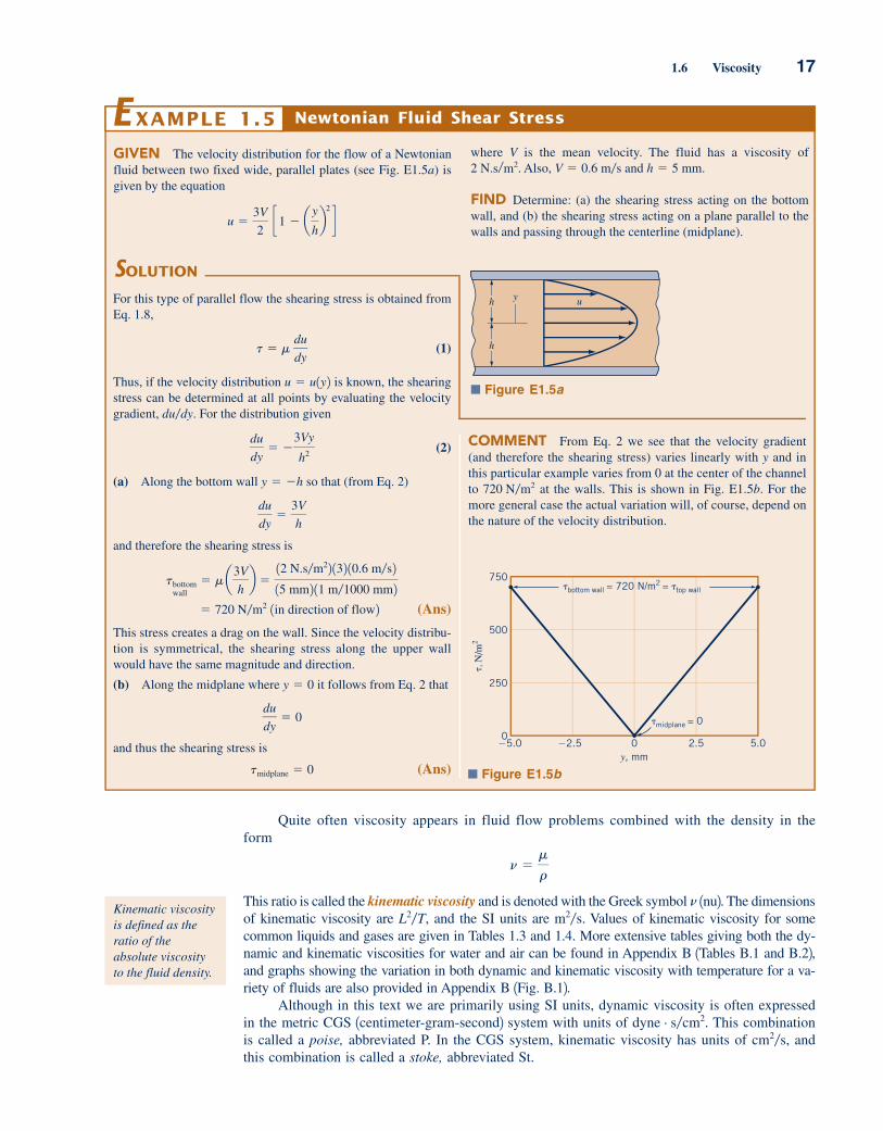
Newtonian Fluid Shear StressEXAMPLE 1.5

GIVEN The velocity distribution for the flow of a Newtonian

fluid between two fixed wide, parallel plates (see Fig. E1.5a) is

given by the equation

u �3V

2 c1 � a

y

hb

2

d

SOLUTION

For this type of parallel flow the shearing stress is obtained from

Eq. 1.8,

(1)

Thus, if the velocity distribution is known, the shearing

stress can be determined at all points by evaluating the velocity

gradient, For the distribution given

(2)

(a) Along the bottom wall so that (from Eq. 2)

and therefore the shearing stress is

(Ans)

This stress creates a drag on the wall. Since the velocity distribu-

tion is symmetrical, the shearing stress along the upper wall

would have the same magnitude and direction.

(b) Along the midplane where it follows from Eq. 2 that

and thus the shearing stress is

(Ans)tmidplane � 0

du

dy� 0

y � 0

� 720 N�m2 1in direction of flow2

tbottomwall

� m a3V

hb �

12 N.s�m22 132 10.6 m�s215 mm2 11 m�1000 mm2

du

dy�

3V

h

y � �h

du

dy� �

3Vy

h2

du�dy.

u � u1y2

t � m du

dy

COMMENT From Eq. 2 we see that the velocity gradient

(and therefore the shearing stress) varies linearly with y and in

this particular example varies from 0 at the center of the channel

to at the walls. This is shown in Fig. E1.5b. For the

more general case the actual variation will, of course, depend on

the nature of the velocity distribution.

720 N�m2

■ Figure E1.5a

h

h

y u

where V is the mean velocity. The fluid has a viscosity of

. Also, and

FIND Determine: (a) the shearing stress acting on the bottom

wall, and (b) the shearing stress acting on a plane parallel to the

walls and passing through the centerline (midplane).

h � 5 mm.V � 0.6 m�s2 N.s�m2

Kinematic viscosityis defined as the ratio of the absolute viscosityto the fluid density.

■ Figure E1.5b

�5.0 �2.5 0 2.5 5.0

750

500

250

0

�, N

/m2

y, mm

�midplane = 0

�bottom wall = 720 N/m2 = �top wall


1.7.1 Bulk Modulus

An important question to answer when considering the behavior of a particular fluid is how eas-

ily can the volume 1and thus the density2 of a given mass of the fluid be changed when there is a

change in pressure? That is, how compressible is the fluid? A property that is commonly used to

characterize compressibility is the bulk modulus, defined as

(1.11)

where dp is the differential change in pressure needed to create a differential change in volume,

of a volume This is illustrated by the figure in the margin. The negative sign is included

since an increase in pressure will cause a decrease in volume. Since a decrease in volume of a

given mass, will result in an increase in density, Eq. 1.11 can also be expressed as

(1.12)

The bulk modulus 1also referred to as the bulk modulus of elasticity2 has dimensions of pressure,

In SI units, values for are usually given as Large values for the bulk modulus indicate

that the fluid is relatively incompressible—that is, it takes a large pressure change to create a small

change in volume. As expected, values of for common liquids are large 1see Table 1.32. For example,

at atmospheric pressure and a temperature of it would require a pressure of 21.5 MPa

to compress a unit volume of water 1%. This result is representative of the compressibility of liquids.

Since such large pressures are required to effect a change in volume, we conclude that liquids can be

considered as incompressible for most practical engineering applications. As liquids are compressed

the bulk modulus increases, but the bulk modulus near atmospheric pressure is usually the one of

interest. The use of bulk modulus as a property describing compressibility is most prevalent when deal-

ing with liquids, although the bulk modulus can also be determined for gases.

1.7.2 Compression and Expansion of Gases

When gases are compressed 1or expanded2, the relationship between pressure and density depends

on the nature of the process. If the compression or expansion takes place under constant temper-

ature conditions 1isothermal process2, then from Eq. 1.7

(1.13)

If the compression or expansion is frictionless and no heat is exchanged with the surroundings

1isentropic process2, then

(1.14)

where k is the ratio of the specific heat at constant pressure, to the specific heat at constant vol-

ume, The two specific heats are related to the gas constant, R, through thecv 1i.e., k � cp�cv2.cp,

p

rk� constant

p

r� constant

15 °C1288 K2Ev

N�m2 1Pa2.Ev

FL�2.

Ev �dp

dr�r

m � rV�,

V�.dV�,

Ev � �dp

dV��V�

Ev,


p

V

p + dp

V – dV

V1.7 Water balloon


This water jet is a blast Usually liquids can be treated as in-

compressible fluids. However, in some applications the com-pressibility of a liquid can play a key role in the operation of a

device. For example, a water pulse generator using compressed

water has been developed for use in mining operations. It can

fracture rock by producing an effect comparable to a conventional

explosive such as gunpowder. The device uses the energy stored

in a water-filled accumulator to generate an ultrahigh-pressure

water pulse ejected through a 10 to 25 mm diameter discharge

valve. At the ultrahigh pressures used (300 to 400 MPa, or 3000

to 4000 atmospheres), the water is compressed (i.e., the volume

reduced) by about 10 to 15%. When a fast-opening valve within

the pressure vessel is opened, the water expands and produces a

jet of water that upon impact with the target material produces an

effect similar to the explosive force from conventional explosives.

Mining with the water jet can eliminate various hazards that arise

with the use of conventional chemical explosives, such as those

associated with the storage and use of explosives and the genera-

tion of toxic gas by-products that require extensive ventilation.

(See Problem 1.110.)

1.7 Compressibility of Fluids

p

Isothermal

Isentropic (k = 1.4)

ρ


1.7 Compressibility of Fluids 19

equation As was the case for the ideal gas law, the pressure in both Eqs. 1.13 and

1.14 must be expressed as an absolute pressure. Values of k for some common gases are given in

Table 1.4 and for air over a range of temperatures, in Appendix B 1B.22. The pressure–density vari-

ations for isothermal and isentropic conditions are illustrated in the margin figure.

With explicit equations relating pressure and density, the bulk modulus for gases can be de-

termined by obtaining the derivative from Eq. 1.13 or 1.14 and substituting the results into

Eq. 1.12. It follows that for an isothermal process

(1.15)and for an isentropic process,

(1.16)

Note that in both cases the bulk modulus varies directly with pressure. For air under standard at-

mospheric conditions with 1abs2 and the isentropic bulk modulus is 142 kPa.

A comparison of this figure with that for water under the same conditions shows

that air is approximately 15,000 times as compressible as water. It is thus clear that in dealing with

gases, greater attention will need to be given to the effect of compressibility on fluid behavior. How-

ever, as will be discussed further in later sections, gases can often be treated as incompressible flu-

ids if the changes in pressure are small.

1Ev � 2150 MPa2k � 1.40,p � 101.3 kPa

Ev � kp

Ev � p

dp�dr

R � cp � cv.

Isentropic Compression of a GasEXAMPLE 1.6

GIVEN 0.03 m3 of air at an absolute pressure of 101.3 kPa is

compressed isentropically to 0.015 m3 by the tire pump shown in

Fig. E1.6a.

FIND What is the final pressure?

SOLUTION

For an isentropic compression

where the subscripts i and f refer to initial and final states,

respectively. Since we are interested in the final pressure, pf,

it follows that

As the volume, is reduced by one-half, the density must

double, since the mass, of the gas remains con-

stant. Thus, with k � 1.40 for air

(Ans)

COMMENT By repeating the calculations for various

values of the ratio of the final volume to the initial volume,

, the results shown in Fig. E1.6b are obtained. Note

that even though air is often considered to be easily com-

pressed (at least compared to liquids), it takes considerable

pressure to significantly reduce a given volume of air as is

done in an automobile engine where the compression ratio is

on the order of � 1/8 � 0.125.V�f �V�i

Vf �Vi

pf � 1221.401101.3 kPa2 � 267 kPa 1abs2

m � r V�.V�.

pf � arf

rib

k

pi

pi

rki

�pf

rkf

■ Figure E1.6a

2700

2400

2100

1800

1500

1200

900

600

300

00 0.2 0.4 0.6 0.8 1.0

p f, kP

a

Vf /Vi

(0.5, 267 kPa)

■ Figure E1.6b

The value of thebulk modulus depends on the typeof process involved.



1800

water

air

1200

600

0 50 1000

c, m

/s

T, �C

The velocity atwhich small distur-bances propagatein a fluid is calledthe speed of sound.

1.7.3 Speed of Sound

Another important consequence of the compressibility of fluids is that disturbances introduced at

some point in the fluid propagate at a finite velocity. For example, if a fluid is flowing in a pipe

and a valve at the outlet is suddenly closed 1thereby creating a localized disturbance2, the effect of

the valve closure is not felt instantaneously upstream. It takes a finite time for the increased pres-

sure created by the valve closure to propagate to an upstream location. Similarly, a loudspeaker

diaphragm causes a localized disturbance as it vibrates, and the small change in pressure created

by the motion of the diaphragm is propagated through the air with a finite velocity. The velocity

at which these small disturbances propagate is called the acoustic velocity or the speed of sound,c. It will be shown in Chapter 11 that the speed of sound is related to changes in pressure and

density of the fluid medium through the equation

(1.17)

or in terms of the bulk modulus defined by Eq. 1.12

(1.18)

Since the disturbance is small, there is negligible heat transfer and the process is assumed to be

isentropic. Thus, the pressure–density relationship used in Eq. 1.17 is that for an isentropic process.

c �B

Ev

r

c �B

dp

dr

Speed of Sound and Mach NumberEXAMPLE 1.7

GIVEN A jet aircraft flies at a speed of 885 km/h at an altitude

of 10,500 m, where the temperature is �54 �C and the specific heat

ratio is k � 1.4.

FIND Determine the ratio of the speed of the aircraft, V, to that

of the speed of sound, c, at the specified altitude.

SOLUTION

From Eq. 1.19 the speed of sound can be calculated as

Since the air speed is

the ratio is

(Ans)

COMMENT This ratio is called the Mach number, Ma. If

Ma 1.0 the aircraft is flying at subsonic speeds, whereas for Ma 1.0 it is flying at supersonic speeds. The Mach number is an impor-

tant dimensionless parameter used in the study of the flow of gases

at high speeds and will be further discussed in Chapters 7 and 11.

By repeating the calculations for different temperatures, the

results shown in Fig. E1.7 are obtained. Because the speed of

V

c�

246 m�s297 m�s

� 0.828

V �1885 km�h2 11000 m�km2

13600 s�h2� 246 m�s

� 297 m/s

� 211.402 1286.9 J�kg.K2 1�54 � 273.152K

c � 2kRT

sound increases with increasing temperature, for a constant

airplane speed, the Mach number decreases as the temperature

increases.

■ Figure E1.7

0.9

1.0

0.8

0.7

0.6

0.5–75 –50 –25 0 25 50 75

Ma

= V

/c

(–54 8C, 0.828)

T, 8C


It is a common observation that liquids such as water and gasoline will evaporate if they are sim-

ply placed in a container open to the atmosphere. Evaporation takes place because some liquid

molecules at the surface have sufficient momentum to overcome the intermolecular cohesive forces

and escape into the atmosphere. If the container is closed with a small air space left above the sur-

face, and this space evacuated to form a vacuum, a pressure will develop in the space as a result

of the vapor that is formed by the escaping molecules. When an equilibrium condition is reached

so that the number of molecules leaving the surface is equal to the number entering, the vapor is

said to be saturated and the pressure that the vapor exerts on the liquid surface is termed the

vapor pressure, . Similarly, if the end of a completely liquid-filled container is moved as shown

in the figure in the margin without letting any air into the container, the space between the liquid

and the end becomes filled with vapor at a pressure equal to the vapor pressure.

Since the development of a vapor pressure is closely associated with molecular activity, the

value of vapor pressure for a particular liquid depends on temperature. Values of vapor pressure for

water at various temperatures can be found in Appendix B 1Table B.12, and the values of vapor pres-

sure for several common liquids at room temperatures are given in Table 1.3.

Boiling, which is the formation of vapor bubbles within a fluid mass, is initiated when the

absolute pressure in the fluid reaches the vapor pressure. As commonly observed in the kitchen,

water at standard atmospheric pressure will boil when the temperature reaches —

that is, the vapor pressure of water at is 101.3 kPa 1abs2. However, if we attempt

to boil water at a higher elevation, say 9000 m above sea level 1the approximate elevation of

Mt. Everest2, where the atmospheric pressure is 30 kPa 1abs2, we find that boiling will start when

the temperature is about At this temperature the vapor pressure of water is 30 kPa

1abs2. For the U.S. Standard Atmosphere 1see Section 2.42, the boiling temperature is a function of

altitude as shown in the figure in the margin. Thus, boiling can be induced at a given pressure act-

ing on the fluid by raising the temperature, or at a given fluid temperature by lowering the pressure.

An important reason for our interest in vapor pressure and boiling lies in the common

observation that in flowing fluids it is possible to develop very low pressure due to the fluid

motion, and if the pressure is lowered to the vapor pressure, boiling will occur. For example, this

phenomenon may occur in flow through the irregular, narrowed passages of a valve or pump.

When vapor bubbles are formed in a flowing fluid, they are swept along into regions of higher

pressure where they suddenly collapse with sufficient intensity to actually cause structural dam-

age. The formation and subsequent collapse of vapor bubbles in a flowing fluid, called cavita-tion, is an important fluid flow phenomenon to be given further attention in Chapters 3 and 7.

69 °C1294 K2.

100 °C1373 K2100 °C 1373 K2

pv

1.8 Vapor Pressure 21

For gases undergoing an isentropic process, 1Eq. 1.162 so that

and making use of the ideal gas law, it follows that

(1.19)

Thus, for ideal gases the speed of sound is proportional to the square root of the absolute temper-

ature. For example, for air at with and , it follows that

The speed of sound in air at various temperatures can be found in Appendix B

1Table B.22. Equation 1.18 is also valid for liquids, and values of can be used to determine the

speed of sound in liquids. For water at and so

that As shown by the figure in the margin, the speed of sound is much higher

in water than in air. If a fluid were truly incompressible the speed of sound would

be infinite. The speed of sound in water for various temperatures can be found in Appendix B

1Table B.12.

1Ev � q 2c � 1481 m�s.

r � 998.2 kg�m320 °C1293 K2, Ev � 2.19 GN�m2

Ev

c � 340.4 m�s.

R � 286.9 J�kg.Kk � 1.4015 °C1288 K2

c � 1kRT

c �B

kp

r

Ev � kp

V1.8 As fast as aspeeding bullet

1.8 Vapor Pressure

Liquid

Liquid

Vapor, pv

A liquid boils whenthe pressure is reduced to the vapor pressure.

2010 15500

30

60

90

120

Boi

ling

tem

pera

ture

, 8C

Altitude, thousandsof meter

In flowing liquids itis possible for thepressure in local-ized regions toreach vapor pres-sure, thereby caus-ing cavitation.



10020 40 60 800Sur

face

ten

sion

, 1

0−2

N/m

6.0

9.07.5

4.5

3.0

1.5

0

Water

Temperature, 8C

V1.9 Floating razorblade


Walking on water Water striders are insects commonly found on

ponds, rivers, and lakes that appear to “walk” on water. A typical

length of a water strider is about 1 cm, and they can cover 100

body lengths in one second. It has long been recognized that

it is surface tension that keeps the water strider from sinking be-

low the surface. What has been puzzling is how they propel them-

selves at such a high speed. They can’t pierce the water surface or

they would sink. A team of mathematicians and engineers from

the Massachusetts Institute of Technology (MIT) applied conven-

tional flow visualization techniques and high-speed video to

examine in detail the movement of the water striders. They found

that each stroke of the insect’s legs creates dimples on the surface

with underwater swirling vortices sufficient to propel it forward.

It is the rearward motion of the vortices that propels the water

strider forward. To further substantiate their explanation, the MIT

team built a working model of a water strider, called Robostrider,

which creates surface ripples and underwater vortices as it moves

across a water surface. Waterborne creatures, such as the water

strider, provide an interesting world dominated by surface tension.

(See Problem 1.97.)

At the interface between a liquid and a gas, or between two immiscible liquids, forces develop

in the liquid surface that cause the surface to behave as if it were a “skin” or “membrane”

stretched over the fluid mass. Although such a skin is not actually present, this conceptual anal-

ogy allows us to explain several commonly observed phenomena. For example, a steel needle

or a razor blade will float on water if placed gently on the surface because the tension devel-

oped in the hypothetical skin supports it. Small droplets of mercury will form into spheres when

placed on a smooth surface because the cohesive forces in the surface tend to hold all the mol-

ecules together in a compact shape. Similarly, discrete bubbles will form in a liquid. (See the

photograph at the beginning of Chapter 1.)

These various types of surface phenomena are due to the unbalanced cohesive forces act-

ing on the liquid molecules at the fluid surface. Molecules in the interior of the fluid mass are

surrounded by molecules that are attracted to each other equally. However, molecules along the

surface are subjected to a net force toward the interior. The apparent physical consequence of this

unbalanced force along the surface is to create the hypothetical skin or membrane. A tensile force

may be considered to be acting in the plane of the surface along any line in the surface. The intensity

of the molecular attraction per unit length along any line in the surface is called the surfacetension and is designated by the Greek symbol 1sigma2. For a given liquid the surface tension

depends on temperature as well as the other fluid it is in contact with at the interface.

The dimensions of surface tension are with SI units of Values of surface tension for

some common liquids 1in contact with air2 are given in Table 1.3 and in Appendix B 1Table B.12for water at various temperatures. As indicated by the figure in the margin, the value of the sur-

face tension decreases as the temperature increases.

N�m.FL�1

s

■ Figure 1.8 Forces acting on one-half of a liquid drop.

Rσ

σR2Δpπ

The pressure inside a drop of fluid can be calculated using the free-body diagram in Fig. 1.8.

If the spherical drop is cut in half 1as shown2, the force developed around the edge due to surface

tension is This force must be balanced by the pressure difference, between the internal

pressure, and the external pressure, acting over the circular area, Thus,

or

(1.20)¢p � pi � pe �2s

R

2pRs � ¢p pR2

pR2.pe,pi,

¢p,2pRs.V1.10 Capillaryrise

1.9 Surface Tension


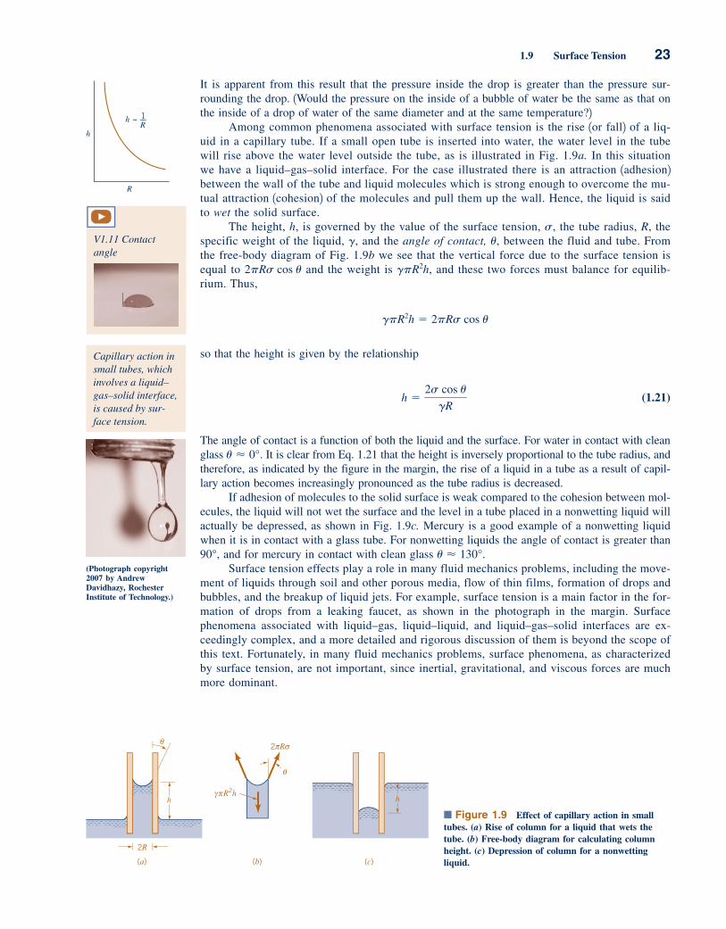
1.9 Surface Tension 23

It is apparent from this result that the pressure inside the drop is greater than the pressure sur-

rounding the drop. 1Would the pressure on the inside of a bubble of water be the same as that on

the inside of a drop of water of the same diameter and at the same temperature?2Among common phenomena associated with surface tension is the rise 1or fall2 of a liq-

uid in a capillary tube. If a small open tube is inserted into water, the water level in the tube

will rise above the water level outside the tube, as is illustrated in Fig. 1.9a. In this situation

we have a liquid–gas–solid interface. For the case illustrated there is an attraction 1adhesion2between the wall of the tube and liquid molecules which is strong enough to overcome the mu-

tual attraction 1cohesion2 of the molecules and pull them up the wall. Hence, the liquid is said

to wet the solid surface.

The height, h, is governed by the value of the surface tension, the tube radius, R, the

specific weight of the liquid, and the angle of contact, between the fluid and tube. From

the free-body diagram of Fig. 1.9b we see that the vertical force due to the surface tension is

equal to and the weight is and these two forces must balance for equilib-

rium. Thus,

so that the height is given by the relationship

(1.21)

The angle of contact is a function of both the liquid and the surface. For water in contact with clean

glass It is clear from Eq. 1.21 that the height is inversely proportional to the tube radius, and

therefore, as indicated by the figure in the margin, the rise of a liquid in a tube as a result of capil-

lary action becomes increasingly pronounced as the tube radius is decreased.

If adhesion of molecules to the solid surface is weak compared to the cohesion between mol-

ecules, the liquid will not wet the surface and the level in a tube placed in a nonwetting liquid will

actually be depressed, as shown in Fig. 1.9c. Mercury is a good example of a nonwetting liquid

when it is in contact with a glass tube. For nonwetting liquids the angle of contact is greater than

and for mercury in contact with clean glass

Surface tension effects play a role in many fluid mechanics problems, including the move-

ment of liquids through soil and other porous media, flow of thin films, formation of drops and

bubbles, and the breakup of liquid jets. For example, surface tension is a main factor in the for-

mation of drops from a leaking faucet, as shown in the photograph in the margin. Surface

phenomena associated with liquid–gas, liquid–liquid, and liquid–gas–solid interfaces are ex-

ceedingly complex, and a more detailed and rigorous discussion of them is beyond the scope of

this text. Fortunately, in many fluid mechanics problems, surface phenomena, as characterized

by surface tension, are not important, since inertial, gravitational, and viscous forces are much

more dominant.

u � 130°.90°,

u � 0°.

h �2s cos u

gR

gpR2h � 2pRs cos u

gpR2h,2pRs cos u

u,g,

s,

hR

R

~ h 1__

Capillary action insmall tubes, whichinvolves a liquid–gas–solid interface,is caused by sur-face tension.

V1.11 Contact angle

■ Figure 1.9 Effect of capillary action in smalltubes. (a) Rise of column for a liquid that wets thetube. (b) Free-body diagram for calculating columnheight. (c) Depression of column for a nonwettingliquid.

π

hR2h

2 R

θ

2R

θ

(a) (b) (c)

γπ

σ

h

(Photograph copyright2007 by AndrewDavidhazy, RochesterInstitute of Technology.)




Spreading of oil spills With the large traffic in oil tankers there

is great interest in the prevention of and response to oil spills. As

evidenced by the famous Exxon Valdez oil spill in Prince

William Sound in 1989, oil spills can create disastrous environ-

mental problems. A more recent example of this type of cata-

strophe is the oil spill that occurred in the Gulf of Mexico in

2010. It is not surprising that much attention is given to the rate

at which an oil spill spreads. When spilled, most oils tend to

spread horizontally into a smooth and slippery surface, called a

slick. There are many factors that influence the ability of an oil

slick to spread, including the size of the spill, wind speed and

direction, and the physical properties of the oil. These properties

include surface tension, specific gravity, and viscosity. The

higher the surface tension the more likely a spill will remain in

place. Since the specific gravity of oil is less than one, it floats

on top of the water, but the specific gravity of an oil can increase

if the lighter substances within the oil evaporate. The higher the

viscosity of the oil, the greater the tendency to stay in one place.

From Eq. 1.21

so that

For water at 1from Table B.12, and

Since it follows that for

and the minimum required tube diameter, D, is

(Ans)

COMMENT By repeating the calculations for various values

of the capillary rise, h, the results shown in Fig. E1.8 are obtained.

D � 2R � 0.0298 m � 29.8 mm

� 0.0149 m

R �210.0728 N�m2 112

19.789 � 103 N�m32 11.0 mm2 110�3 m�mm2

h � 1.0 mm,u � 0°g � 9.789 kN�m3.

s � 0.0728 N�m20 °C

R �2s cos u

gh

h �2s cos u

gR

Note that as the allowable capillary rise is decreased, the diame-

ter of the tube must be significantly increased. There is always

some capillarity effect, but it can be minimized by using a large

enough diameter tube.

SOLUTION

0.5 1h, mm

D, m

m

1.5 200

20

40

60

80

100

(1 mm, 29.8 mm)

■ Figure E1.8

1.10 A Brief Look Back in History

Some of the earliestwritings that per-tain to modern fluidmechanics can betraced back to theancient Greek civi-lization and subse-quent Roman Empire.

Before proceeding with our study of fluid mechanics, we should pause for a moment to consider

the history of this important engineering science. As is true of all basic scientific and engineering

disciplines, their actual beginnings are only faintly visible through the haze of early antiquity. But

we know that interest in fluid behavior dates back to the ancient civilizations. Through necessity

there was a practical concern about the manner in which spears and arrows could be propelled

through the air, in the development of water supply and irrigation systems, and in the design of

boats and ships. These developments were, of course, based on trial-and-error procedures without

any knowledge of mathematics or mechanics. However, it was the accumulation of such empirical

knowledge that formed the basis for further development during the emergence of the ancient Greek

civilization and the subsequent rise of the Roman Empire. Some of the earliest writings that per-

tain to modern fluid mechanics are those of Archimedes 1287–212 B.C.2, a Greek mathematician

and inventor who first expressed the principles of hydrostatics and flotation. Elaborate water sup-

ply systems were built by the Romans during the period from the fourth century B.C. through the

early Christian period, and Sextus Julius Frontinus 1A.D. 40–1032, a Roman engineer, described these

Capillary Rise in a TubeEXAMPLE 1.8

GIVEN Pressures are sometimes determined by measuring the

height of a column of liquid in a vertical tube.

FIND What diameter of clean glass tubing is required so that

the rise of water at in a tube due to capillary action 1as op-

posed to pressure in the tube2 is less than h � 1.0 mm?

20 °C


1.10 A Brief Look Back in History 25

systems in detail. However, for the next 1000 years during the Middle Ages 1also referred to as the

Dark Ages2, there appears to have been little added to further understanding of fluid behavior.

As shown in Fig. 1.10, beginning with the Renaissance period 1about the fifteenth century2a rather continuous series of contributions began that forms the basis of what we consider to be

the science of fluid mechanics. Leonardo da Vinci 11452–15192 described through sketches and

writings many different types of flow phenomena. The work of Galileo Galilei 11564–16422marked

the beginning of experimental mechanics. Following the early Renaissance period and during the

seventeenth and eighteenth centuries, numerous significant contributions were made. These include

theoretical and mathematical advances associated with the famous names of Newton, Bernoulli,

Euler, and d’Alembert. Experimental aspects of fluid mechanics were also advanced during this

period, but unfortunately the two different approaches, theoretical and experimental, developed

along separate paths. Hydrodynamics was the term associated with the theoretical or mathemati-

cal study of idealized, frictionless fluid behavior, with the term hydraulics being used to describe

the applied or experimental aspects of real fluid behavior, particularly the behavior of water. Fur-

ther contributions and refinements were made to both theoretical hydrodynamics and experimen-

tal hydraulics during the nineteenth century, with the general differential equations describing fluid

motions that are used in modern fluid mechanics being developed in this period. Experimental hy-

draulics became more of a science, and many of the results of experiments performed during the

nineteenth century are still used today.

At the beginning of the twentieth century, both the fields of theoretical hydrodynamics

and experimental hydraulics were highly developed, and attempts were being made to unify the

two. In 1904 a classic paper was presented by a German professor, Ludwig Prandtl 11875–

19532, who introduced the concept of a “fluid boundary layer,” which laid the foundation for

the unification of the theoretical and experimental aspects of fluid mechanics. Prandtl’s idea

was that for flow next to a solid boundary a thin fluid layer 1boundary layer2 develops in which

friction is very important, but outside this layer the fluid behaves very much like a frictionless

fluid. This relatively simple concept provided the necessary impetus for the resolution of the

conflict between the hydrodynamicists and the hydraulicists. Prandtl is generally accepted as

the founder of modern fluid mechanics.

Also, during the first decade of the twentieth century, powered flight was first successfully

demonstrated with the subsequent vastly increased interest in aerodynamics. Because the design

of aircraft required a degree of understanding of fluid flow and an ability to make accurate pre-

dictions of the effect of airflow on bodies, the field of aerodynamics provided a great stimulus for

the many rapid developments in fluid mechanics that took place during the twentieth century.

As we proceed with our study of the fundamentals of fluid mechanics, we will continue to note

the contributions of many of the pioneers in the field. Table 1.5 provides a chronological listing of

some of these contributors and reveals the long journey that makes up the history of fluid mechan-

ics. This list is certainly not comprehensive with regard to all past contributors but includes those

who are mentioned in this text. As mention is made in succeeding chapters of the various individu-

als listed in Table 1.5, a quick glance at this table will reveal where they fit into the historical chain.

Year

200019001800170016001500140013001200

Geoffrey Taylor

Theodor von Karman

Ludwig Prandtl

Osborne Reynolds

Ernst Mach

George Stokes

Leonardo da Vinci

Galileo Galilei

Isaac Newton

Daniel Bernoulli

Leonhard Euler

Louis Navier

Jean Poiseuille

■ Figure 1.10 Time line of some contributors to the science of fluid mechanics.

The rich history offluid mechanics isfascinating, andmany of the contri-butions of thepioneers in the fieldare noted in thesucceedingchapters.



ARCHIMEDES 1287– 212 B.C.2Established elementary principles of buoyancy andflotation.

SEXTUS JULIUS FRONTINUS 1A.D. 40–1032Wrote treatise on Roman methods of waterdistribution.

LEONARDO da VINCI 11452–15192Expressed elementary principle of continuity;observed and sketched many basic flowphenomena; suggested designs for hydraulicmachinery.

GALILEO GALILEI 11564–16422Indirectly stimulated experimental hydraulics;revised Aristotelian concept of vacuum.

EVANGELISTA TORRICELLI 11608–16472Related barometric height to weight ofatmosphere, and form of liquid jet to trajectoryof free fall.

BLAISE PASCAL 11623–16622Finally clarified principles of barometer, hydraulicpress, and pressure transmissibility.

ISAAC NEWTON 11642–17272Explored various aspects of fluid resistance—inertial, viscous, and wave; discovered jetcontraction.

HENRI de PITOT 11695–17712Constructed double-tube device to indicate watervelocity through differential head.

DANIEL BERNOULLI 11700–17822Experimented and wrote on many phases of fluidmotion, coining name “hydrodynamics”; devisedmanometry technique and adapted primitive energyprinciple to explain velocity-head indication;proposed jet propulsion.

LEONHARD EULER 11707–17832First explained role of pressure in fluid flow;formulated basic equations of motion and so-called Bernoulli theorem; introduced concept of cavitation and principle of centrifugalmachinery.

JEAN le ROND d’ALEMBERT 11717–17832Originated notion of velocity and acceleration com-ponents, differential expression of continuity, andparadox of zero resistance to steady nonuniformmotion.

ANTOINE CHEZY 11718–17982Formulated similarity parameter for predicting flowcharacteristics of one channel from measurements onanother.

GIOVANNI BATTISTA VENTURI 11746–18222Performed tests on various forms of mouthpieces—in particular, conical contractions and expansions.

LOUIS MARIE HENRI NAVIER 11785–18362Extended equations of motion to include“molecular” forces.

AUGUSTIN LOUIS de CAUCHY 11789–18572Contributed to the general field of theoreticalhydrodynamics and to the study of wave motion.

GOTTHILF HEINRICH LUDWIG HAGEN11797–18842Conducted original studies of resistance in andtransition between laminar and turbulent flow.

JEAN LOUIS POISEUILLE 11799–18692Performed meticulous tests on resistance of flowthrough capillary tubes.

HENRI PHILIBERT GASPARD DARCY 11803–18582Performed extensive tests on filtration and piperesistance; initiated open-channel studies carried outby Bazin.

JULIUS WEISBACH 11806–18712Incorporated hydraulics in treatise on engineeringmechanics, based on original experiments;noteworthy for flow patterns, nondimensionalcoefficients, weir, and resistance equations.

WILLIAM FROUDE 11810–18792Developed many towing-tank techniques, inparticular the conversion of wave and boundary layerresistance from model to prototype scale.

ROBERT MANNING 11816–18972Proposed several formulas for open-channel resistance.

GEORGE GABRIEL STOKES 11819–19032Derived analytically various flow relationshipsranging from wave mechanics to viscous resistance—particularly that for the settling of spheres.

ERNST MACH 11838–19162One of the pioneers in the field of supersonicaerodynamics.

OSBORNE REYNOLDS 11842–19122Described original experiments in many fields—cavitation, river model similarity, pipe resistance—and devised two parameters for viscous flow; adaptedequations of motion of a viscous fluid to meanconditions of turbulent flow.

JOHN WILLIAM STRUTT, LORD RAYLEIGH11842–19192Investigated hydrodynamics of bubble collapse,wave motion, jet instability, laminar flow analogies,and dynamic similarity.

VINCENZ STROUHAL 11850–19222Investigated the phenomenon of “singing wires.”

EDGAR BUCKINGHAM 11867–19402Stimulated interest in the United States in the use ofdimensional analysis.

MORITZ WEBER 11871–19512Emphasized the use of the principles of similitude influid flow studies and formulated a capillaritysimilarity parameter.

LUDWIG PRANDTL 11875–19532Introduced concept of the boundary layer and isgenerally considered to be the father of present-dayfluid mechanics.

Table 1.5

Chronological Listing of Some Contributors to the Science of Fluid Mechanics Noted in the Texta

Leonardo da Vinci

Isaac Newton

Daniel Bernoulli

Ernst Mach

Osborne Reynolds


It is, of course, impossible to summarize the rich history of fluid mechanics in a few para-

graphs. Only a brief glimpse is provided, and we hope it will stir your interest. References 2 to 5

are good starting points for further study, and in particular Ref. 2 provides an excellent, broad, eas-

ily read history. Try it—you might even enjoy it!

1.11 Chapter Summary and Study Guide 27

LEWIS FERRY MOODY 11880–19532Provided many innovations in the field of hydraulicmachinery. Proposed a method of correlating piperesistance data that is widely used.

THEODOR VON KÁRMÁN11881–19632One of the recognized leaders of twentieth centuryfluid mechanics. Provided major contributions to our

understanding of surface resistance, turbulence, andwake phenomena.

PAUL RICHARD HEINRICH BLASIUS11883–19702One of Prandtl’s students who provided an analyticalsolution to the boundary layer equations. Alsodemonstrated that pipe resistance was related to theReynolds number.

Table 1.5 (continued)

aUsed by permission of IIHR—Hydroscience & Engineering, The University of Iowa.

Ludwig Prandtl

1.11 Chapter Summary and Study Guide

This introductory chapter discussed several fundamental aspects of fluid mechanics. Methods

for describing fluid characteristics both quantitatively and qualitatively are considered. For a

quantitative description, units are required, and in this text, International (SI) System units are

used. For the qualitative description the concept of dimensions is introduced in which basic di-

mensions such as length, L, time, T, and mass, M, are used to provide a description of various

quantities of interest. The use of dimensions is helpful in checking the generality of equations,

as well as serving as the basis for the powerful tool of dimensional analysis discussed in de-

tail in Chapter 7.

Various important fluid properties are defined, including fluid density, specific weight,

specific gravity, viscosity, bulk modulus, speed of sound, vapor pressure, and surface tension.

The ideal gas law is introduced to relate pressure, temperature, and density in common gases,

along with a brief discussion of the compression and expansion of gases. The distinction be-

tween absolute and gage pressure is introduced and this important idea is explored more fully

in Chapter 2.

The following checklist provides a study guide for this chapter. When your study of the en-

tire chapter and end-of-chapter exercises has been completed you should be able to

write out meanings of the terms listed here in the margin and understand each of the related

concepts. These terms are particularly important and are set in italic, bold, and color type

in the text.

determine the dimensions of common physical quantities.

determine whether an equation is a general or restricted homogeneous equation.

use SI system of units.

calculate the density, specific weight, or specific gravity of a fluid from a knowledge of any

two of the three.

calculate the density, pressure, or temperature of an ideal gas (with a given gas constant)

from a knowledge of any two of the three.

relate the pressure and density of a gas as it is compressed or expanded using Eqs. 1.13

and 1.14.

use the concept of viscosity to calculate the shearing stress in simple fluid flows.

calculate the speed of sound in fluids using Eq. 1.18 for liquids and Eq. 1.19 for gases.

fluid units basic dimensions dimensionally

homogeneous density specific weight specific gravity ideal gas law absolute pressure gage pressureno-slip conditionrate of shearing strainabsolute viscosityNewtonian fluid non-Newtonian fluidkinematic viscositybulk modulus speed of sound vapor pressure surface tension



References

1. Reid, R. C., Prausnitz, J. M., and Sherwood, T. K., The Properties of Gases and Liquids, 3rd Ed.,McGraw-Hill, New York, 1977.

2. Rouse, H. and Ince, S., History of Hydraulics, Iowa Institute of Hydraulic Research, Iowa City, 1957,Dover, New York, 1963.

3. Tokaty, G. A., A History and Philosophy of Fluid Mechanics, G. T. Foulis and Co., Ltd., Oxfordshire,Great Britain, 1971.

4. Rouse, H., Hydraulics in the United States 1776–1976, Iowa Institute of Hydraulic Research, IowaCity, Iowa, 1976.

5. Garbrecht, G., ed., Hydraulics and Hydraulic Research—A Historical Review, A. A. Balkema,Rotterdam, Netherlands, 1987.

6. Brenner, M. P., Shi, X. D., Eggens, J., and Nagel, S. R., Physics of Fluids, Vol. 7, No. 9, 1995.

7. Shi, X. D., Brenner, M. P., and Nagel, S. R., Science, Vol. 265, 1994.

determine whether boiling or cavitation will occur in a liquid using the concept of vapor

pressure.

use the concept of surface tension to solve simple problems involving liquid–gas or liquid–

solid–gas interfaces.

Some of the important equations in this chapter are:

Specific weight (1.5)

Specific gravity (1.6)

Ideal gas law (1.7)

Newtonian fluid shear stress (1.8)

Bulk modulus (1.11)

Speed of sound in an ideal gas (1.19)

Capillary rise in a tube (1.21)h �2s cos u

gR

c � 1kRT

Ev � �dp

dV��V�

t � m du

dy

r �p

RT

SG �r

rH2O@4 °C

g � rg

Review Problems

Go to Appendix G (WileyPLUS or the book’s website, www.wiley.com/college/munson) for a set of review problems with answers. Detailed solutions can be found in the Student Solution

Manual and Study Guide for Fundamentals of Fluid Mechanics, byMunson et al. © 2013 John Wiley and Sons, Inc.).

Problem available in WileyPLUS at instructor’s discretion.

Tutoring problem available in WileyPLUS at instructor’s discretion.

Problem is related to a chapter video available in WileyPLUS.

Problem to be solved with aid of programmable calculator or computer.

Open-ended problem that requires critical thinking. These problems require various assumptions to provide the necessary

input data. There are not unique answers to these problems.

GO

*†


Problems 29

Which figure best describes the variation of shear stress with dis-tance from the plate?

Additional conceptual questions are available in WileyPLUS atthe instructor’s discretion.

y

ShearStress

τ

0 y

ShearStress

τ

0 y

ShearStress

τ

0 y

ShearStress

τ

0 y

ShearStress

τ

0

0

Heighty

Velocity u

1.1C The correct statement for the definition of density is

a) Density is the mass per unit volume.

b) Density is the volume per unit mass.

c) Density is the weight per unit volume.

d) Density is the weight divided by gravity.

e) Density is the mass divided by the weight.

1.2C Given the following equation where p is pressure in N/m2,� is the specific weight in kg/m3, V is the magnitude of velocityin m/s, g is in m/s2, and z is height in meters. If values aresubstituted into the equation, will the correct value of C bedetermined?

a) Yes if the constant C has units of m.

b) Yes if the constant C is dimensionless.

c) No, the equation cannot produce the correct value of C.

d) Yes if the constant C has units of m and the specific weight ismultiplied by the conversion factor from kg to N.

1.3C The no-slip condition is:

a) An experimental observation that the velocity of a fluid incontact with a solid surface is equal to the velocity of thesurface.

b) Valid only for liquids.

p

g�

V 2

2g� z � C

c) Useful only for very low density gases.

d) Indicates that two solids in contact will not slip if the joiningforce is large.

1.4C In fluids, the shearing strain rate for a Newtonian fluidhas dimensions of:

a) L/T2. c) L2/T.

b) 1/T. d) L2/T2.

1.5C The laminar velocity profile for a Newtonian fluid is shownbelow.

du

dy

Problems

Note: Unless specific values of required fluid properties are givenin the problem statement, use the values found in the tables on theinside of the front cover. Answers to the even-numbered problemsare listed at the end of the book. The Lab Problems as well as thevideos that accompany problems can be accessed in WileyPLUSor the book’s website, www.wiley.com/college/munson.

Section 1.2 Dimensions, Dimensional Homogeneity,and Units

1.1 The force, F, of the wind blowing against a building is givenby where V is the wind speed, the density ofthe air, A the cross-sectional area of the building, and CD is a con-stant termed the drag coefficient. Determine the dimensions ofthe drag coefficient.

1.2 Determine the dimensions, in both the FLT system and theMLT system, for (a) the product of mass times velocity, (b) the prod-uct of force times volume, and (c) kinetic energy divided by area.

1.3 Verify the dimensions, in both the FLT and MLT systems, ofthe following quantities which appear in Table 1.1: (a) volume, (b)acceleration, (c) mass, (d) moment of inertia (area), and (e) work.

1.4 Determine the dimensions, in both the FLT system and theMLT system, for (a) the product of force times acceleration, (b) theproduct of force times velocity divided by area, and (c) momentumdivided by volume.

rF � CDrV2 A�2,

Conceptual Questions

1.5 Verify the dimensions, in both the FLT and MLT systems, ofthe following quantities which appear in Table 1.1: (a) angularvelocity, (b) energy, (c) moment of inertia (area), (d) power, and(e) pressure.

1.6 Verify the dimensions, in both the FLT system and the MLTsystem, of the following quantities which appear in Table 1.1:(a) frequency, (b) stress, (c) strain, (d) torque, and (e) work.

1.7 If u is a velocity, x a length, and t a time, what are the dimensions 1in the MLT system2 of (a) (b)(c)

1.8 Verify the dimensions, in both the FLT system and the MLTsystem, of the following quantities which appear in Table 1.1:(a) acceleration, (b) stress, (c) moment of a force, (d) volume,and (e) work.

1.9 If p is a pressure, V a velocity, and r a fluid density, whatare the dimensions (in the MLT system) of (a) p/r, (b) pVr, and(c) ?

1.10 If P is a force and x a length, what are the dimensions (inthe FLT system) of (a) dP/dx, (b) d3P/dx3, and (c) dx?

1.11 If V is a velocity, a length, and a fluid property (the kinematic viscosity) having dimensions of which of thefollowing combinations are dimensionless: (a) (b)(c) (d) V�/n?V 2n,

V/�n,V/n,L2T �1,n/

�P

p�rV 2

� 10u�0t2 dx?02u�0x0t, and0u�0t,


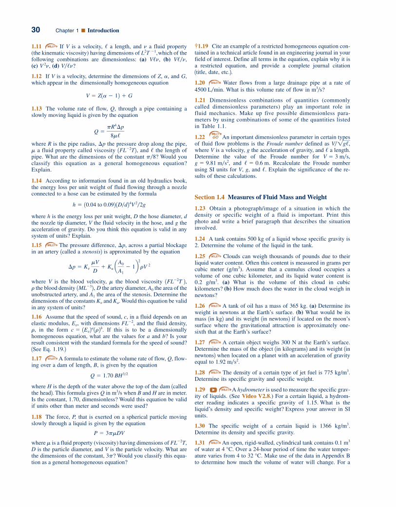
†1.19 Cite an example of a restricted homogeneous equation con-tained in a technical article found in an engineering journal in yourfield of interest. Define all terms in the equation, explain why it isa restricted equation, and provide a complete journal citation 1title, date, etc.2.

1.20 Water flows from a large drainage pipe at a rate of

What is this volume rate of flow in ?

1.21 Dimensionless combinations of quantities (commonlycalled dimensionless parameters) play an important role influid mechanics. Make up five possible dimensionless para-meters by using combinations of some of the quantities listedin Table 1.1.

1.22 An important dimensionless parameter in certain typesof fluid flow problems is the Froude number defined as where V is a velocity, g the acceleration of gravity, and � a length.Determine the value of the Froude number for

and Recalculate the Froude numberusing SI units for V, g, and Explain the significance of the re-sults of these calculations.

Section 1.4 Measures of Fluid Mass and Weight

1.23 Obtain a photograph/image of a situation in which thedensity or specific weight of a fluid is important. Print thisphoto and write a brief paragraph that describes the situationinvolved.

1.24 A tank contains 500 kg of a liquid whose specific gravity is2. Determine the volume of the liquid in the tank.

1.25 Clouds can weigh thousands of pounds due to theirliquid water content. Often this content is measured in grams percubic meter (g/m3). Assume that a cumulus cloud occupies a volume of one cubic kilometer, and its liquid water content is 0.2 g/m3. (a) What is the volume of this cloud in cubickilometers? (b) How much does the water in the cloud weigh innewtons?

1.26 A tank of oil has a mass of 365 kg. (a) Determine itsweight in newtons at the Earth’s surface. (b) What would be itsmass 1in kg2 and its weight 1in newtons2 if located on the moon’ssurface where the gravitational attraction is approximately one-sixth that at the Earth’s surface?

1.27 A certain object weighs 300 N at the Earth’s surface.Determine the mass of the object 1in kilograms2 and its weight 1innewtons2 when located on a planet with an acceleration of gravityequal to

1.28 The density of a certain type of jet fuel is 775 kg/m3.Determine its specific gravity and specific weight.

1.29 A hydrometer is used to measure the specific grav-ity of liquids. (See Video V2.8.) For a certain liquid, a hydrom-eter reading indicates a specific gravity of 1.15. What is theliquid’s density and specific weight? Express your answer in SIunits.

1.30 The specific weight of a certain liquid is 1366 kg/m3.Determine its density and specific gravity.

1.31 An open, rigid-walled, cylindrical tank contains of water at Over a 24-hour period of time the water temper-ature varies from 4 to Make use of the data in Appendix Bto determine how much the volume of water will change. For a

32 °C.4 °C.

0.1 m3

1.92 m�s2.

/./ � 0.6 m.g � 9.81 m�s2,

V � 3 m�s,

V�1g/,

GO

m3�s4500 L�min.

1.11 If V is a velocity, a length, and a fluid property (the kinematic viscosity) having dimensions of which of thefollowing combinations are dimensionless: (a) (b)(c) (d)

1.12 If V is a velocity, determine the dimensions of Z, a, and G,which appear in the dimensionally homogeneous equation

1.13 The volume rate of flow, Q, through a pipe containing aslowly moving liquid is given by the equation

where R is the pipe radius, the pressure drop along the pipe,a fluid property called viscosity , and the length of

pipe. What are the dimensions of the constant Would youclassify this equation as a general homogeneous equation?Explain.

1.14 According to information found in an old hydraulics book,the energy loss per unit weight of fluid flowing through a nozzleconnected to a hose can be estimated by the formula

where h is the energy loss per unit weight, D the hose diameter, dthe nozzle tip diameter, V the fluid velocity in the hose, and g theacceleration of gravity. Do you think this equation is valid in anysystem of units? Explain.

1.15 The pressure difference, across a partial blockagein an artery 1called a stenosis2 is approximated by the equation

where V is the blood velocity, the blood viscosity the blood density the artery diameter, the area of the

unobstructed artery, and the area of the stenosis. Determine the dimensions of the constants and Would this equation be validin any system of units?

1.16 Assume that the speed of sound, c, in a fluid depends on anelastic modulus, , with dimensions and the fluid density,

in the form If this is to be a dimensionally homogeneous equation, what are the values for a and b? Is your result consistent with the standard formula for the speed of sound?1See Eq. 1.19.2

1.17 A formula to estimate the volume rate of flow, Q, flow-ing over a dam of length, B, is given by the equation

where H is the depth of the water above the top of the dam 1calledthe head2. This formula gives Q in m3/s when B and H are in meter.Is the constant, 1.70, dimensionless? Would this equation be validif units other than meter and seconds were used?

1.18 The force, P, that is exerted on a spherical particle movingslowly through a liquid is given by the equation

where m is a fluid property (viscosity) having dimensions of FL�2T,D is the particle diameter, and V is the particle velocity. What arethe dimensions of the constant, 3p? Would you classify this equa-tion as a general homogeneous equation?

P � 3pmDV

Q � 1.70 BH3�2

c � 1Ev2a1r2b.r,

FL�2,Ev

Ku.Kv

A1

A01ML�32, Dr1FL�2T 2,m

¢p � Kv mV

D� Ku a

A0

A1

� 1b2

rV 2

¢p,

h � 10.04 to 0.092 1D�d24V 2�2g

p�8?/1FL�2T2m

¢p

Q �pR4¢p

8m/

V � Z1a � 12 � G

V�/n?V 2n,V/�n,V/n,

L2T �1,n/



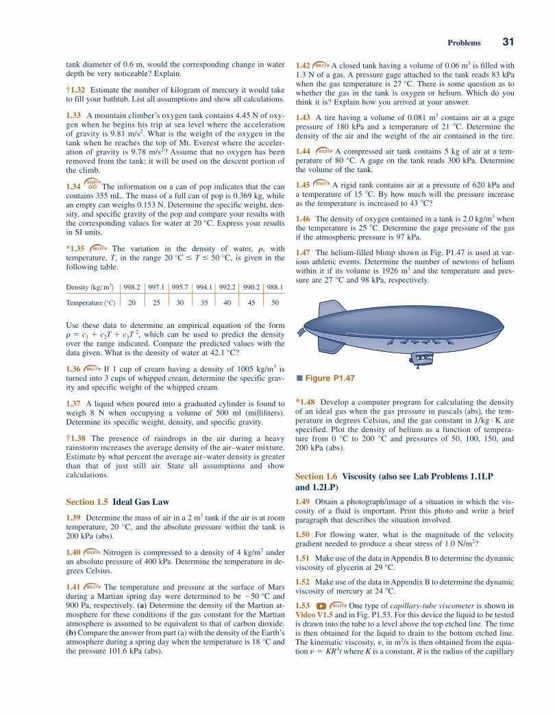
tank diameter of 0.6 m, would the corresponding change in waterdepth be very noticeable? Explain.

†1.32 Estimate the number of kilogram of mercury it would taketo fill your bathtub. List all assumptions and show all calculations.

1.33 A mountain climber’s oxygen tank contains 4.45 N of oxy-gen when he begins his trip at sea level where the accelerationof gravity is 9.81 m/s2. What is the weight of the oxygen in thetank when he reaches the top of Mt. Everest where the acceler-ation of gravity is 9.78 m/s2? Assume that no oxygen has beenremoved from the tank; it will be used on the descent portion ofthe climb.

1.34 The information on a can of pop indicates that the cancontains 355 mL. The mass of a full can of pop is 0.369 kg, whilean empty can weighs 0.153 N. Determine the specific weight, den-sity, and specific gravity of the pop and compare your results withthe corresponding values for water at Express your resultsin SI units.

*1.35 The variation in the density of water, withtemperature, T, in the range is given in thefollowing table.

Density 1kg m32 998.2 997.1 995.7 994.1 992.2 990.2 988.1

Temperature 20 25 30 35 40 45 50

Use these data to determine an empirical equation of the form, which can be used to predict the density

over the range indicated. Compare the predicted values with thedata given. What is the density of water at

1.36 If 1 cup of cream having a density of 1005 kg/m3 isturned into 3 cups of whipped cream, determine the specific grav-ity and specific weight of the whipped cream.

1.37 A liquid when poured into a graduated cylinder is found toweigh 8 N when occupying a volume of 500 ml (milliliters).Determine its specific weight, density, and specific gravity.

†1.38 The presence of raindrops in the air during a heavyrainstorm increases the average density of the air–water mixture.Estimate by what percent the average air–water density is greaterthan that of just still air. State all assumptions and showcalculations.

Section 1.5 Ideal Gas Law

1.39 Determine the mass of air in a 2 m3 tank if the air is at roomtemperature, 20 °C, and the absolute pressure within the tank is200 kPa (abs).

1.40 Nitrogen is compressed to a density of 4 kg/m3 underan absolute pressure of 400 kPa. Determine the temperature in de-grees Celsius.

1.41 The temperature and pressure at the surface of Marsduring a Martian spring day were determined to be and900 Pa, respectively. (a) Determine the density of the Martian at-mosphere for these conditions if the gas constant for the Martianatmosphere is assumed to be equivalent to that of carbon dioxide.(b) Compare the answer from part (a) with the density of the Earth’satmosphere during a spring day when the temperature is andthe pressure 101.6 kPa (abs).

18 °C

�50 °C

42.1 °C?

r � c1 � c2T � c3T 2

1°C2

�

20 °C � T � 50 °C,r,

20 °C.

GO

1.42 A closed tank having a volume of is filled with 1.3 N of a gas. A pressure gage attached to the tank reads 83 kPawhen the gas temperature is There is some question as towhether the gas in the tank is oxygen or helium. Which do youthink it is? Explain how you arrived at your answer.

1.43 A tire having a volume of 0.081 m3 contains air at a gagepressure of 180 kPa and a temperature of 21 �C. Determine thedensity of the air and the weight of the air contained in the tire.

1.44 A compressed air tank contains 5 kg of air at a tem-perature of 80 °C. A gage on the tank reads 300 kPa. Determinethe volume of the tank.

1.45 A rigid tank contains air at a pressure of 620 kPa anda temperature of 15 �C. By how much will the pressure increaseas the temperature is increased to 43 �C?

1.46 The density of oxygen contained in a tank is 2.0 kg/m3 whenthe temperature is 25 �C. Determine the gage pressure of the gasif the atmospheric pressure is 97 kPa.

1.47 The helium-filled blimp shown in Fig. P1.47 is used at var-ious athletic events. Determine the number of newtons of heliumwithin it if its volume is 1926 m3 and the temperature and pres-sure are 27 °C and 98 kPa, respectively.

27 °C.

0.06 m3

■ Figure P1.47

*1.48 Develop a computer program for calculating the densityof an ideal gas when the gas pressure in pascals 1abs2, the tem-perature in degrees Celsius, and the gas constant in arespecified. Plot the density of helium as a function of tempera-ture from 0 °C to 200 °C and pressures of 50, 100, 150, and 200 kPa (abs).

Section 1.6 Viscosity (also see Lab Problems 1.1LP and 1.2LP)

1.49 Obtain a photograph/image of a situation in which the vis-cosity of a fluid is important. Print this photo and write a briefparagraph that describes the situation involved.

1.50 For flowing water, what is the magnitude of the velocitygradient needed to produce a shear stress of 1.0 N/m2?

1.51 Make use of the data in Appendix B to determine the dynamicviscosity of glycerin at

1.52 Make use of the data in Appendix B to determine the dynamicviscosity of mercury at 24 �C.

1.53 One type of capillary-tube viscometer is shown inVideo V1.5 and in Fig. P1.53. For this device the liquid to be testedis drawn into the tube to a level above the top etched line. The timeis then obtained for the liquid to drain to the bottom etched line.The kinematic viscosity, �, in m2/s is then obtained from the equa-tion where K is a constant, R is the radius of the capillaryn � KR4t

29 °C.

J�kg # K

Problems 31



tube in mm, and t is the drain time in seconds. When glycerin at20 �C is used as a calibration fluid in a particular viscometer, thedrain time is 1430 s. When a liquid having a density of 970 kg/m3

is tested in the same viscometer the drain time is 900 s. What isthe dynamic viscosity of this liquid?

Plot these data and fit a second-order polynomial to the data usinga suitable graphing program. What is the apparent viscosity of thisfluid when the rate of shearing strain is 70 ? Is this apparentviscosity larger or smaller than that for water at the sametemperature?

1.60 Water flows near a flat surface and some mea-surements of the water velocity, u, parallel to the surface, at dif-ferent heights, y, above the surface are obtained. At the surface

. After an analysis of the data, the lab technician reports thatthe velocity distribution in the range is given bythe equation

with u in m/s when y is in m. (a) Do you think that this equa-tion would be valid in any system of units? Explain. (b) Do youthink this equation is correct? Explain. You may want to look atVideo 1.4 to help you arrive at your answer.

1.61 Calculate the Reynolds numbers for the flow of wa-ter and for air through a 4 mm diameter tube, if the mean velocityis 3 m s and the temperature is in both cases (see Exam-ple 1.4). Assume the air is at standard atmospheric pressure.

1.62 SAE 30 oil at 15 �C flows through a 5 cm diameter pipe witha mean velocity of 1.5 m/s. Determine the value of the Reynoldsnumber (see Example 1.4).

1.63 For air at standard atmospheric pressure the values of theconstants that appear in the Sutherland equation 1Eq. 1.102 are

and Use thesevalues to predict the viscosity of air at and and com-pare with values given in Table B.4 in Appendix B.

*1.64 Use the values of viscosity of air given in Table B.4 at tem-peratures of 0, 20, 40, 60, 80, and to determine the con-stants C and S which appear in the Sutherland equation 1Eq. 1.102.Compare your results with the values given in Problem 1.68. 1Hint:Rewrite the equation in the form

and plot versus T. From the slope and intercept of this curve,C and S can be obtained.2

1.65 The viscosity of a fluid plays a very important role indetermining how a fluid flows. (See Video V1.3.) The value of theviscosity depends not only on the specific fluid but also on the fluidtemperature. Some experiments show that when a liquid, under theaction of a constant driving pressure, is forced with a low veloc-ity, V, through a small horizontal tube, the velocity is given by theequation . In this equation K is a constant for a given tubeand pressure, and � is the dynamic viscosity. For a particular liq-uid of interest, the viscosity is given by Andrade’s equation (Eq.1.11) with and . By what per-centage will the velocity increase as the liquid temperature is in-creased from 4 �C to 37 �C? Assume all other factors remainconstant.

*1.66 Use the value of the viscosity of water given in Table B.2at temperatures of 0, 20, 40, 60, 80, and to determine theconstants D and B which appear in Andrade’s equation 1Eq. 1.112.Calculate the value of the viscosity at and compare with thevalue given in Table B.2. 1Hint: Rewrite the equation in the form

ln m � 1B2 1

T� ln D

50 °C

100 °C

B � 2222 KD � 0.000023 N.s�m2

V � K�m

T 3� 2�m

T 3� 2

m� a

1

Cb T �

S

C

100 °C

90 °C10 °CS � 110.4 K.C � 1.458 � 10�6 kg� 1m # s # K1�22

30 °C�

u � 0.81 � 9.2y � 4.1 � 103y3

0 6 y 6 0.1 my � 0

s�1

Etched lines

Glassstrengthening

bridge

Capillarytube

■ Figure P1.53

1.54 The viscosity of a soft drink was determined byusing a capillary tube viscometer similar to that shown in Fig. P1.53 and Video V1.5. For this device the kinematic viscosity,�, is directly proportional to the time, t, that it takes for a givenamount of liquid to flow through a small capillary tube. That is,

. The following data were obtained from regular pop anddiet pop. The corresponding measured specific gravities are alsogiven. Based on these data, by what percent is the absolute vis-cosity, �, of regular pop greater than that of diet pop?

Regular pop Diet pop

t(s) 377.8 300.3

SG 1.044 1.003

1.55 Determine the ratio of the dynamic viscosity of water to airat a temperature of 60 °C. Compare this value with the corre-sponding ratio of kinematic viscosities. Assume the air is at stan-dard atmospheric pressure.

1.56 The kinematic viscosity and specific gravity of a liquid are3.5 � 10�4 m2/s and 0.79, respectively. What is the dynamic vis-cosity of the liquid in SI units?

1.57 A liquid has a specific weight of 945 kg/m3 and a dynamic viscosity of 131.67 N.s/m2. Determine its kinematicviscosity.

1.58 The kinematic viscosity of oxygen at and a pressureof 150 kPa 1abs2 is 0.104 stokes. Determine the dynamic viscosityof oxygen at this temperature and pressure.

*1.59 Fluids for which the shearing stress, �, is not linearlyrelated to the rate of shearing strain, ��, are designated as non-Newtonian fluids. Such fluids are commonplace and can exhibitunusual behavior, as shown in Video V1.6. Some experimental dataobtained for a particular non-Newtonian fluid at 27 �C are shownbelow.

� (kPa) 0 0.1 0.37 0.89 1.5

�� (s�1) 0 50 100 150 200

20 °C

n � Kt


Problems 33

1.72 A 25 mm diameter shaft is pulled through a cylindri-cal bearing as shown in Fig. P1.72. The lubricant that fills the 0.3 mm gap between the shaft and bearing is an oil having a kine-matic viscosity of and a specific gravity of 0.91.Determine the force P required to pull the shaft at a velocity of 3 m/s. Assume the velocity distribution in the gap is linear.

8.0 � 10�4 m2�s

■ Figure P1.71

0.5 m

LubricantBearing

ShaftP

■ Figure P1.72

■ Figure P1.74

V0.1 mm gap

20°

u__U

y__h

y2__h22 –=

Uh

y u

■ Figure P1.75

and plot ln versus From the slope and intercept of this curve,B and D can be obtained. If a nonlinear curve-fitting program isavailable, the constants can be obtained directly from Eq. 1.11 with-out rewriting the equation.2

1.67 For a certain liquid m� 0.0034 N.s/m2 at 4 �C and m� 0.009N.s/m2 at 66 �C. Make use of these data to determine the constantsD and B which appear in Andrade’s equation (Eq. 1.11). Whatwould be the viscosity at 27 �C?

1.68 For a parallel plate arrangement of the type shown inFig. 1.5 it is found that when the distance between plates is 2 mm,a shearing stress of 150 Pa develops at the upper plate when it ispulled at a velocity of 1 m/s. Determine the viscosity of the fluidbetween the plates. Express your answer in SI units.

1.69 Two flat plates are oriented parallel above a fixed lower plateas shown in Fig. P1.69. The top plate, located a distance b abovethe fixed plate, is pulled along with speed V. The other thin plateis located a distance cb, where 0 c 1, above the fixed plate.This plate moves with speed V1, which is determined by the vis-cous shear forces imposed on it by the fluids on its top and bot-tom. The fluid on the top is twice as viscous as that on the bottom.Plot the ratio V1/V as a function of c for 0 c 1.

GO

1�T.m

1.75 A layer of water flows down an inclined fixed surfacewith the velocity profile shown in Fig. P1.75. Determine the mag-nitude and direction of the shearing stress that the water exerts onthe fixed surface for .U � 2 m�s and h � 0.1 m

b

cb

2μ

μ

V

V1

■ Figure P1.69

1.70 There are many fluids that exhibit non-Newtonian behavior (see, for example, Video V1.6). For a given fluid the dis-tinction between Newtonian and non-Newtonian behavior is usu-ally based on measurements of shear stress and rate of shearingstrain. Assume that the viscosity of blood is to be determined by measurements of shear stress, �, and rate of shearing strain,du/dy, obtained from a small blood sample tested in a suitable vis-cometer. Based on the data given below, determine if the blood isa Newtonian or non-Newtonian fluid. Explain how you arrived atyour answer.

�(N/m2) 0.04 0.06 0.12 0.18 0.30 0.52 1.12 2.10

du/dy ( ) 2.25 4.50 11.25 22.5 45.0 90.0 225 450

1.71 The sled shown in Fig. P1.71 slides along on a thinhorizontal layer of water between the ice and the runners. Thehorizontal force that the water puts on the runners is equal to 5.3 Nwhen the sled’s speed is 15 m/s. The total area of both runners in con-tact with the water is , and the viscosity of the water is

Determine the thickness of the water layer underthe runners. Assume a linear velocity distribution in the water layer.168 � 10�5 N.s�m2.

0.007 m2

s�1

1.73 A piston having a diameter of 13.92 cm and a length of 24.13 cm slides downward with a velocity V through a verticalpipe. The downward motion is resisted by an oil film between thepiston and the pipe wall. The film thickness is 0.005 cm, and thecylinder weighs 0.23 kg. Estimate V if the oil viscosity is 0.766N.s/m2. Assume the velocity distribution in the gap is linear.

1.74 A 10 kg block slides down a smooth inclined surfaceas shown in Fig. P1.74. Determine the terminal velocity of theblock if the 0.1 mm gap between the block and the surface con-tains SAE 30 oil at 15 °C. Assume the velocity distribution in thegap is linear, and the area of the block in contact with the oil is0.1 m2.

1.76 A thin layer of glycerin flows down an inclined, wide platewith the velocity distribution shown in Fig. P1.76. For h �0.75 cm and a � 20�, determine the surface velocity, U. Note thatfor equilibrium, the component of weight acting parallel to the platesurface must be balanced by the shearing force developed alongthe plate surface. In your analysis assume a unit plate width.



and the stationary base. Determine the frictional torque on the shaftwhen it rotates at 5000 rpm.

■ Figure P1.81

Liquid

Fixedouter

cylinder�

ω

�

Rotatinginner

cylinder

Ri

Ro

■ Figure P1.80

0.5 cm

0.0025 cm

5000 rpm

30°

= 0.479 N.s/m2µ

1.81 The viscosity of liquids can be measured through the use of arotating cylinder viscometer of the type illustrated in Fig. P1.81. Inthis device the outer cylinder is fixed and the inner cylinder is rotatedwith an angular velocity, The torque required to develop ismeasured and the viscosity is calculated from these two measure-ments. (a) Develop an equation relating and Neglectend effects and assume the velocity distribution in the gap is linear.(b) The following torque-angular velocity data were obtained with arotating cylinder viscometer of the type discussed in part (a).

Torque 17.8 35.3 53.6 71.5 87.9 106.5

Angular 1.0 2.0 3.0 4.0 5.0 6.0velocity

For this viscometer and Make use of these data and a standard curve-fitting program to de-termine the viscosity of the liquid contained in the viscometer.

/ � 12.7 cm.Ri � 6.22 cm,Ro � 6.35 cm,

1rad�s2

1N.m2

Ri.m, v, t, /, Ro,

�tv.

■ Figure P1.78

10,000 rpm0.012 mm

Rotating disc50 mm

5 mm dia.Stationary reader head

*1.77 Standard air flows past a flat surface, and velocitymeasurements near the surface indicate the followingdistribution:

y 1m2 1.5�10–3 3�10–3 6�10–3 12�10–3 18�10–3 24�10–3

u 0.23 0.46 0.92 1.94 3.11 4.39

The coordinate y is measured normal to the surface and u is thevelocity parallel to the surface. (a) Assume the velocity distribu-tion is of the form

and use a standard curve-fitting technique to determine the con-stants and (b) Make use of the results of part 1a2 to deter-mine the magnitude of the shearing stress at the wall andat

1.78 A new computer drive is proposed to have a disc, asshown in Fig. P1.78. The disc is to rotate at 10,000 rpm, and thereader head is to be positioned 0.012 mm above the surface of thedisc. Estimate the shearing force on the reader head as a result ofthe air between the disc and the head.

y � 0.05 ft.1y � 02

C2.C1

u � C1y � C2y3

1m�s2

1.82 One type of rotating cylinder viscometer, called a Stormerviscometer, uses a falling weight, �, to cause the cylinder to ro-tate with an angular velocity, v, as illustrated in Fig. P1.82. Forthis device the viscosity, m, of the liquid is related to � and vthrough the equation � � Kmv, where K is a constant that depends only on the geometry (including the liquid depth) of the

u__U

y__h

y2__h22 –=

U

yu

h

α

■ Figure P1.76

1.79 The space between two 15 cm long concentric cylin-ders is filled with glycerin Theinner cylinder has a radius of 7.6 cm and the gap width betweencylinders is 0.25 cm. Determine the torque and the power requiredto rotate the inner cylinder at The outer cylinder isfixed. Assume the velocity distribution in the gap to be linear.

1.80 A pivot bearing used on the shaft of an electrical in-strument is shown in Fig. P1.80. An oil with a viscosity of � �0.479 N.s/m2 fills the 0.0025 cm gap between the rotating shaft

180 rev�min.

1viscosity � 407 � 10�3 N.s�m22.


Problems 35

viscometer. The value of K is usually determined by using a cali-bration liquid (a liquid of known viscosity).(a) Some data for a particular Stormer viscometer, obtained usingglycerin at 20 �C as a calibration liquid, are given below. Plot val-ues of the weight as ordinates and values of the angular velocity asabscissae. Draw the best curve through the plotted points and de-termine K for the viscometer.

�(kg) 0.1 0.3 0.5 0.7 1

v (rev/s) 0.53 1.59 2.79 3.83 5.49

(b) A liquid of unknown viscosity is placed in the same viscometerused in part (a), and the data given below are obtained. Determinethe viscosity of this liquid.

�(kg) 0.02 0.05 0.1 0.15 0.2

v (rev/s) 0.72 1.89 3.73 5.44 7.42

1.88 A rigid-walled cubical container is completely filled with wa-ter at 4 �C and sealed. The water is then heated to 38 �C. Deter-mine the pressure that develops in the container when the waterreaches this higher temperature. Assume that the volume of thecontainer remains constant and the value of the bulk modulus ofthe water remains constant and equal to 2.1 GPa.

1.89 In a test to determine the bulk modulus of a liquid it wasfound that as the absolute pressure was changed from 103 to 21 MPa the volume decreased from 167.8 to 166.13 cm3. Deter-mine the bulk modulus for this liquid.

1.90 Estimate the increase in pressure (in kPa) required todecrease a unit volume of mercury by 0.1%.

1.91 A volume of water is contained in a rigid con-tainer. Estimate the change in the volume of the water when a pis-ton applies a pressure of 35 MPa.

1.92 Determine the speed of sound at 20 °C in (a) air, (b) helium,and (c) natural gas (methane). Express your answer in m/s.

1.93 Calculate the speed of sound in m/s for (a) gasoline, (b) mer-cury, and (c) seawater.

1.94 Air is enclosed by a rigid cylinder containing a piston.A pressure gage attached to the cylinder indicates an initial read-ing of 172 kPa. Determine the reading on the gage when the pis-ton has compressed the air to one-third its original volume. Assume the compression process to be isothermal and the local atmospheric pressure to be 101.3 kPa.

1.95 Repeat Problem 1.94 if the compression process takes placewithout friction and without heat transfer (isentropic process).

1.96 Carbon dioxide at and 300 kPa absolute pres-sure expands isothermally to an absolute pressure of 165 kPa. Determine the final density of the gas.

1.97 Oxygen at 30 �C and 300 kPa absolute pressure expandsisothermally to an absolute pressure of 120 kPa. Determine the final density of the gas.

1.98 Natural gas at and standard atmosphericpressure of 101.3 kPa (abs) is compressed isentropically to a newabsolute pressure of 483 kPa. Determine the final density andtemperature of the gas.

1.99 Compare the isentropic bulk modulus of air at 101 kPa 1abs2with that of water at the same pressure.

*1.100 Develop a computer program for calculating the final gagepressure of gas when the initial gage pressure, initial and final vol-umes, atmospheric pressure, and the type of process 1isothermal orisentropic2 are specified. Check your program against the resultsobtained for Problem 1.94.

1.101 Often the assumption is made that the flow of a certain fluidcan be considered as incompressible flow if the density of the fluidchanges by less than 2%. If air is flowing through a tube such thatthe air pressure at one section is 62 kPa and at a downstream sec-tion it is 59 kPa at the same temperature, do you think that thisflow could be considered an incompressible flow? Support youranswer with the necessary calculations. Assume standard atmos-pheric pressure.

1.102 An important dimensionless parameter concernedwith very high-speed flow is the Mach number, defined as V/c,where V is the speed of the object such as an airplane or projec-tile, and c is the speed of sound in the fluid surrounding the ob-ject. For a projectile traveling at 1290 km/h through air at 10 �C

21 °C

30 °C

1 m3

Rotating plate

0.25 cm gap

Torque

■ Figure P1.83

Liquid

Fixed outercylinder

Weight

ω

� Rotatinginner

cylinder

■ Figure P1.82

1.83 A 30 cm diameter circular plate is placed over a fixedbottom plate with a 0.25 cm gap between the two plates filled withglycerin as shown in Fig. P1.83. Determine the torque required torotate the circular plate slowly at 2 rpm. Assume that the velocitydistribution in the gap is linear and that the shear stress on the edgeof the rotating plate is negligible.

†1.84 Vehicle shock absorbers damp out oscillations caused byroad roughness. Describe how a temperature change may affect theoperation of a shock absorber.

1.85 Some measurements on a blood sample at indi-cate a shearing stress of 0.52 for a corresponding rate of shear-ing strain of . Determine the apparent viscosity of the bloodand compare it with the viscosity of water at the same temperature.

Section 1.7 Compressibility of Fluids

1.86 Obtain a photograph/image of a situation in which the com-pressibility of a fluid is important. Print this photo and write a briefparagraph that describes the situation involved.

1.87 A sound wave is observed to travel through a liquidwith a speed of 1500 m/s. The specific gravity of the liquid is 1.5.Determine the bulk modulus for this fluid.

200 s�1N�m2

37 °C


1.116 Estimate the excess pressure inside a raindrop having a di-ameter of 3 mm.

1.117 What is the difference between the pressure inside a soapbubble and atmospheric pressure for a 7.5 cm diameter bubble? Assume the surface tension of the soap film to be 70% of that ofwater at 21 �C.

1.118 As shown in Video V1.9, surface tension forcescan be strong enough to allow a double-edge steel razor blade to“float” on water, but a single-edge blade will sink. Assume that thesurface tension forces act at an angle � relative to the water sur-face as shown in Fig. P1.118. (a) The mass of the double-edgeblade is , and the total length of its sides is 206 mm.Determine the value of � required to maintain equilibrium betweenthe blade weight and the resultant surface tension force. (b) The mass of the single-edge blade is , and thetotal length of its sides is 154 mm. Explain why this blade sinks.Support your answer with the necessary calculations.

2.61 � 10�3 kg

0.64 � 10�3 kg


and standard atmospheric pressure, what is the value of the Machnumber?

1.103 Jet airliners typically fly at altitudes between approximately0 to 12200 m. Make use of the data in Appendix C to show on agraph how the speed of sound varies over this range.

1.104 (See Fluids in the News article titled “This waterjet is a blast,” Section 1.7.1.) By what percent is the volume ofwater decreased if its pressure is increased to an equivalent to304 MPa?

Section 1.8 Vapor Pressure1.105 During a mountain climbing trip it is observed thatthe water used to cook a meal boils at 90 °C rather than the stan-dard 100 °C at sea level. At what altitude are the climbers prepar-ing their meal? (See Tables B.2 and C.2 for data needed to solvethis problem.)

1.106 When a fluid flows through a sharp bend, low pres-sures may develop in localized regions of the bend. Estimate theminimum absolute pressure 1in kPa2 that can develop without caus-ing cavitation if the fluid is water at

1.107 A partially filled closed tank contains ethyl alcohol at 20 �C. If the air above the alcohol is evacuated, what is the mini-mum absolute pressure that develops in the evacuated space?

1.108 Estimate the minimum absolute pressure 1in pascals2that can be developed at the inlet of a pump to avoid cavitation ifthe fluid is carbon tetrachloride at

1.109 When water at flows through a converging section of pipe, the pressure decreases in the direction of flow. Estimate the minimum absolute pressure that can develop withoutcausing cavitation. Express your answer in SI units.

1.110 At what atmospheric pressure will water boil at Express your answer in SI units.

Section 1.9 Surface Tension

1.111 Obtain a photograph/image of a situation in which the sur-face tension of a fluid is important. Print this photo and write abrief paragraph that describes the situation involved.

1.112 When a 2 mm diameter tube is inserted into a liquid in an open tank, the liquid is observed to rise 10 mm above thefree surface of the liquid (see Video V1.10). The contact angle be-tween the liquid and the tube is zero, and the specific weight ofthe liquid is 1.2 � 104 N/m3. Determine the value of the surfacetension for this liquid.

1.113 An open 2 mm diameter tube is inserted into a pan of ethylalcohol, and a similar 4 mm diameter tube is inserted into a panof water. In which tube will the height of the rise of the fluid col-umn due to capillary action be the greatest? Assume the angle ofcontact is the same for both tubes.

1.114 Small droplets of carbon tetrachloride at areformed with a spray nozzle. If the average diameter of the dropletsis , what is the difference in pressure between the insideand outside of the droplets?

1.115 A 12 mm diameter jet of water discharges vertically intothe atmosphere. Due to surface tension the pressure inside the jetwill be slightly higher than the surrounding atmospheric pressure.Determine this difference in pressure.

200 mm

20 °C

35 °C?

70 °C

20 °C.

70 °C.

■ Figure P1.118

Surface tensionforce

Blade θ

1.119 To measure the water depth in a large open tank with opaquewalls, an open vertical glass tube is attached to the side of the tank.The height of the water column in the tube is then used as a mea-sure of the depth of water in the tank. (a) For a true water depthin the tank of 1 m, make use of Eq. 1.21 (with ) to deter-mine the percent error due to capillarity as the diameter of the glasstube is changed. Assume a water temperature of 27 �C. Show yourresults on a graph of percent error versus tube diameter, D, in therange . (b) If you want the error to be lessthan 1%, what is the smallest tube diameter allowed?

1.120 Under the right conditions, it is possible, dueto surface tension, to have metal objects float on water. (SeeVideo V1.9.) Consider placing a short length of a small diame-ter steel (g � 77 kN/m3) rod on a surface of water. What is themaximum diameter that the rod can have before it will sink? As-sume that the surface tension forces act vertically upward. Note:A standard paper clip has a diameter of 0.09 cm. Partially un-fold a paper clip and see if you can get it to float on water. Dothe results of this experiment support your analysis?

1.121 An open, clean glass tube, having a diameter of3 mm, is inserted vertically into a dish of mercury at (seeVideo V1.10). How far will the column of mercury in the tube be depressed?

1.122 An open, clean glass tube is insertedvertically into a pan of water (see Video V1.10). What tube diameter is needed if the water level in the tube is to rise one tubediameter (due to surface tension)?

1.123 Determine the height that water at 15 °C willrise due to capillary action in a clean, 0.6 cm diameter tube (seeVideo V1.10). What will be the height if the diameter is reducedto 0.03 cm?

1.124 Two vertical, parallel, clean glass plates are spaced a dis-tance of 2 mm apart. If the plates are placed in water, how highwill the water rise between the plates due to capillary action?

1u � 0°2

20 °C

GO

0.25 cm 6 D 6 2.5 cm

u � 0°


Problems 37

■ Figure P1.125

1.125 (See Fluids in the News article titled “Walking onwater,” Section 1.9.) (a) The water strider bug shown in Fig.P1.125 is supported on the surface of a pond by surface tensionacting along the interface between the water and the bug’s legs.Determine the minimum length of this interface needed to supportthe bug. Assume the bug weighs and the surface tensionforce acts vertically upwards. (b) Repeat part (a) if surface tensionwere to support a person weighing 750 N.

10�4 N

which is located in WileyPLUS or on the book’s website, www. wiley.com/college/munson.

■ Lifelong Learning Problems

1.1 LL Although there are numerous non-Newtonian fluids thatoccur naturally (quicksand and blood among them), with the ad-vent of modern chemistry and chemical processing, many newmanufactured non-Newtonian fluids are now available for a vari-ety of novel applications. Obtain information about the discoveryand use of newly developed non-Newtonian fluids. Summarizeyour findings in a brief report.

1.2 LL For years, lubricating oils and greases obtained by refin-ing crude oil have been used to lubricate moving parts in a widevariety of machines, motors, and engines. With the increasing costof crude oil and the potential for the reduced availability of it, theneed for non-petroleum-based lubricants has increased consider-ably. Obtain information about non-petroleum-based lubricants.Summarize your findings in a brief report.

1.3 LL It is predicted that nanotechnology and the use of nanosized objects will allow many processes, procedures, and productsthat, as of now, are difficult for us to comprehend. Among newnanotechnology areas is that of nano scale fluid mechanics. Fluidbehavior at the nano scale can be entirely different than that forthe usual everyday flows with which we are familiar. Obtain in-formation about various aspects of nano fluid mechanics. Sum-marize your findings in a brief report.

■ FE Exam Problems

Sample FE (Fundamentals of Engineering) exam question for fluidmechanics are provided in WileyPLUS or on the book’s website,www.wiley.com/college/munson.

■ Lab Problems

1.1LP This problem involves the use of a Stormer viscometer todetermine whether a fluid is a Newtonian or a non-Newtonian fluid.To proceed with this problem, go to Appendix H, which is locatedin WileyPLUS or on the book’s website, www.wiley.com/col-lege/munson.

1.2LP This problem involves the use of a capillary tube vis-cometer to determine the kinematic viscosity of water as a functionof temperature. To proceed with this problem, go to Appendix H,


1introduction - wiley

Documents