epicEPIC Documentation

Release 1.3

Rafael J. F. Marcondes

Jul 20, 2018

Contents

1 Welcome to the EPIC user’s guide! 21.1 Why EPIC? . . . . . . . . . . . . . . . . . . . . . . . . . . . . . . . . . . . . . . 2

2 How to install 32.1 Setting up a virtual environment . . . . . . . . . . . . . . . . . . . . . . . . . . . 32.2 Defining your custom EPIC home folder (optional) . . . . . . . . . . . . . . . . . 42.3 Installing EPIC . . . . . . . . . . . . . . . . . . . . . . . . . . . . . . . . . . . . 4

3 The Cosmology calculator 53.1 The interactive calculator . . . . . . . . . . . . . . . . . . . . . . . . . . . . . . . 53.2 The cosmological models . . . . . . . . . . . . . . . . . . . . . . . . . . . . . . . 83.3 The datasets . . . . . . . . . . . . . . . . . . . . . . . . . . . . . . . . . . . . . . 133.4 The calculator GUI . . . . . . . . . . . . . . . . . . . . . . . . . . . . . . . . . . 15

4 The MCMC module 194.1 Introduction to MCMC and the Bayesian method . . . . . . . . . . . . . . . . . . 194.2 Before starting . . . . . . . . . . . . . . . . . . . . . . . . . . . . . . . . . . . . 214.3 Running MCMC . . . . . . . . . . . . . . . . . . . . . . . . . . . . . . . . . . . 244.4 MCMC from the GUI . . . . . . . . . . . . . . . . . . . . . . . . . . . . . . . . . 34

5 Acknowledgments 37

arX

iv:1

712.

0026

3v4

[as

tro-

ph.I

M]

20

Jul 2

018

1 Welcome to the EPIC user’s guide!

Easy Parameter Inference in Cosmology (EPIC) is my implementation in Python of a MCMCcode for Bayesian inference of parameters of cosmological models and model comparison via thecomputation of Bayesian evidences.

1.1 Why EPIC?

I started to develop EPIC as a means of learning how parameter inference can be made with MarkovChain Monte Carlo, rather than trying to decipher other codes or using them as black boxes. Theprogram has fulfilled this purposed and went on to incorporate a few cosmological observables thatI have actually employed in some of my publications. Now I release this code in the hope it canbe useful to students seeking to learn some of the methods used in Observational Cosmology andeven to use it for their own work. It still lacks some important features. A Boltzmann solver is notavailable. It is possible that I will integrate it with CLASS1 to make it more useful for advancedresearch. Stay tuned for more.

On the other hand, development is active and with recent versions it is now possible not only touse EPIC’s Cosmology Calculator but also run MCMC simulations from a nice graphical interface.You can also, check out these other features:

• Cross-platform: the code runs on Python 3 in any operating system.

• EPIC features a Cosmology Calculator that also supports a few models other than the stan-dard ΛCDM model. The list of models include interacting dark energy and some dark energyequation-of-state parametrizations. The code can output some key distance calculations andcompare them between different models over a range of redshifts, generating extensivelycustomizable plots.

• It uses Python’s multiprocessing library for evolution of chains in parallel in MCMCsimulations. The separate processes can communicate with each other through somemultiprocessing utilities, which made possible the implementation of the Parallel Tem-pering algorithm.2 This method is capable of detecting and accurately sampling posteriordistributions that present two or more separated peaks.

• Convergence between independent chains is tested with the multivariate version of the Gel-man and Rubin test, a very robust method.

• Also, the plots are beautiful and can be customized to a great extent directly from the com-mand line or from the graphical interface, without having to change the code. You can viewtriangle plots with marginalized distributions of parameters, predefined derived parameters,

1 Lesgourgues, J. “The Cosmic Linear Anisotropy Solving System (CLASS) I: Overview”. arXiv:1104.2932[astro-ph.IM]; Blas, D., Lesgourgues, J., Tram, T. “The Cosmic Linear Anisotropy Solving System (CLASS). PartII: Approximation schemes”. Journal of Cosmology and Astroparticle Physics 07 (2011) 034.

2 Removed in current version. If you need to use Parallel Tempering, please use version 1.0.4 of EPIC.

two-dimensional joint-posterior distributions, autocorrelation plots, cross-correlation plots,sequence plots, convergence diagnosis and more.

Try it now!

2 How to install

You can obtain this program either from PyPi (installing with pip) or cloning the public repos-itory from BitBucket. But first, it is recommended that you make these changes inside a virtualenvironment.

2.1 Setting up a virtual environment

On Unix systems

The preferred way is using Python3’s venv module, available in Python 3.3 and superior versions.When choosing this option on Unix systems, the main script epic.py will be executable fromany location. In a directory of your preference, create a virtual Python environment (for example,named EPIC-env) and activate it with:

$ python3 -m venv EPIC-env$ source EPIC-env/bin/activate

When you finish using the environment and want to leave it you can just use $ deactivate. Toactivate it again, which you need in a new session, just run the activation command above (thesecond line only). More details about Python3’s venv here.

Alternatively, you can install pyenv and pyenv-virtualenv, which let you create a virtual environ-ment and even choose another version of Python to install. This is done with:

$ pyenv virtualenv 3.6.1 EPIC-env # or choose other version you like.$ pyenv activate EPIC-env # use 'pyenv deactivate' to deactivate it.

Note that this version of EPIC is not compatible with Python 2 anymore.

On Windows

EPIC is supported on Windows through the Conda system. Download and install Miniconda3.Then, from the Anaconda prompt, create and activate your environment with:

$ conda create -n EPIC-env python$ conda activate EPIC-env

2.2 Defining your custom EPIC home folder (optional)

By default, data from the MCMC simulations will be saved to a folder named simulations in thesame location of the input .ini file used in each simulation. You can have a common location forall results by defining an environment variable. This makes sense since the output files can be bigand you might want to store them in a separate driver.

To do this, before installing EPIC, set the variable EPIC_USER_PATH to the location of your pref-erence. On Unix systems, add the following line to your ~/.bashrc or ~/.bashprofile or~/.profile file:

export EPIC_USER_PATH="/path/to/folder/"

so the variable will be defined in every session. On Windows, open Control Panel, go to System andSecurity, System, Advanced system settings, Environment Variables. In the section User variablesfor (your user), click the New button, browse to the directory that you want to set as EPIC’s homeand create the variable with the name EPIC_USER_PATH.

2.3 Installing EPIC

From PyPi

The easiest way to install this program is to get it from PyPi. It is also the most recommendedsince it can be easily updated when new versions come out. Inside your virtual environment, run:

$ pip install epic-code

You are now good to go. During the installation, some .ini files will be extracted to the EPIC’shome folder in your home folder or in EPIC_USER_PATH if you defined it before. If you used venvand your system is Unix, you may be able to launch EPIC’s graphical interface just by running:

$ epic.py

from any location. In other configurations, when this cannot be achieved, the script epic.py willbe exported to the home folder so you can execute it from that location with:

$ python epic.py

To check and install updates if available, just run:

$ pip install --upgrade epic-code

from inside your environment.

Cloning the git repository

If you plan to contribute to this program you can clone the git repository at https://bitbucket.org/

rmarcondes/epic, running:

$ git clone https://bitbucket.org/rmarcondes/epic.git

After downloading the repository, cd into the epic folder and install the program with:

$ pip install -e .

This should be repeated as you edit the program unless you are always running it from the EPICfolder. To use modified code from the python interactive interpreter you need to install it again.

3 The Cosmology calculator

Starting with version 1.1, there is now a module available that makes it easy for the user to performcalculations on the background cosmology given a specific model. A few classes of models arepredefined. Each of these have also defined what are their components, but also allowing somevariations. For example, the ΛCDM model requires at least cold dark matter (cdm) and cosmo-logical constant (lambda), but one can also include baryonic fluid (baryons), or treat both mattercomponents together by specifying the composed species matter. It is also possible to includephotons or radiation. For models of interaction between dark matter and dark energy (cde),the former is labelled idm and the latter ide or ilambda in the case that its equation-of-stateparameter is still −1 (in which the model is then labelled cde_lambda) rather than a free parame-ter or presents evolution described by some function. The models available and their componentsspecification are defined in the file EPIC/cosmology/model_recipes.ini. The fluids containedin this file are in turn defined in EPIC/cosmology/available_species.ini, where propertieslike the type of equation of state, the parameters and other relevant informations are set.

In version 1.2, a graphical user interface (GUI) for this cosmology calculator has been added toEPIC. After describing how all calculations are done in EPIC, we present the GUI in the lastsection.

3.1 The interactive calculator

We start (preferably on jupyter notebook) importing the module and creating our cosmology object:

>>> from EPIC.cosmology import cosmic_objects as cosmo>>> LCDM = cosmo.CosmologicalSetup('lcdm')

Only the label of the model is really needed here, since the essentials are already predefined in theprogram, as mentioned above. With this, one can explore the properties assigned to the object. Forexample, LCDM.model will print lcdm. LCDM.species is a dictionary of Fluid objects identified

by the components labels, in this case cdm and lambda. There is also a dedicated class for anequation-of-state parameter or function, which becomes an attribute of its fluid. We can assess itsvalue, type, etc. LCDM.species['lambda'].EoS.value will print -1.

But let us proceed in a slightly different way, setting up our model with some options. Since wepredominantly work with flat cosmologies (in fact, curvature is not supported yet in the currentversion), the flatness condition is imposed in the density parameter of one of the fluids. We willchoose the dark energy density parameter to be the derived parameter, but we could have chosendark matter as well. Also, by default, the code prefers to work with physical densities (for exampleΩc0h2) rather than the common Ωc0. You can change this with the option physical=False. Wewill add the radiation and matter fluids. Note that this will override the optional inclusion ofbaryons and remove them, if given. The radiation fluid is parametrized by the temperature of thecosmic microwave background. The model will have three free parameters: the physical densityparameter of matter (Ωm0h2), the CMB temperature (Tγ, which we usually keep fixed) and theHubble parameter h; and one derived parameter, which is the density parameter of the cosmologicalconstant, ΩΛh2.

>>> LCDM = cosmo.CosmologicalSetup(... 'lcdm',... optional_species=['baryons', 'radiation'], # baryons will be ignored→because of 'matter' in the line bellow... combined_species=['matter'],... derived='lambda'... )

We can then obtain the solution to the background cosmology with EPIC.

Solving the background cosmology

It is as simple as this:

>>> LCDM.solve_background(accepts_default=True)

Normally, a set of parameters would be given to this function in the form of a dic-tionary with the parameters’ labels as keys, like in parameter_space='Oc0': 0.26,'Ob0': 0.048, 'Or0':8e-5, 'H0':67.8. However, we can also ommit it and turn onthe option accepts_default and then the default values defined in the EPIC/cosmology/default_parameter_values.ini file will be used for the parameters. Next, we plot the energydensities and density parameters. Here I do it in a jupyter notebook with the help of this simplefunction below:

>>> %matplotlib inline>>> import matplotlib.pyplot as plt>>> import numpy as np>>> plt.rcParams['text.usetex'] = True

(continues on next page)

(continued from previous page)

>>> plt.rcParams['font.size'] = 16>>> plt.rcParams['figure.dpi'] = 144

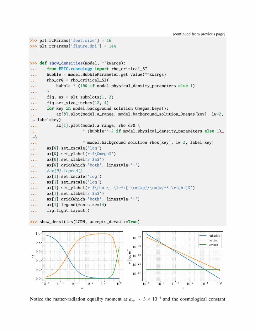
>>> def show_densities(model, **kwargs):... from EPIC.cosmology import rho_critical_SI... hubble = model.HubbleParameter.get_value(**kwargs)... rho_cr0 = rho_critical_SI(... hubble * (100 if model.physical_density_parameters else 1)... )... fig, ax = plt.subplots(1, 2)... fig.set_size_inches(12, 4)... for key in model.background_solution_Omegas.keys():... ax[0].plot(model.a_range, model.background_solution_Omegas[key], lw=2,→ label=key)... ax[1].plot(model.a_range, rho_cr0 \... * (hubble**-2 if model.physical_density_parameters else 1)→\... * model.background_solution_rhos[key], lw=2, label=key)... ax[0].set_xscale('log')... ax[0].set_ylabel(r'$\Omega$')... ax[0].set_xlabel(r'$a$')... ax[0].grid(which='both', linestyle=':')... #ax[0].legend()... ax[1].set_xscale('log')... ax[1].set_yscale('log')... ax[1].set_ylabel(r'$\rho \, \left[ \rmkg/\rmm^3 \right]$')... ax[1].set_xlabel(r'$a$')... ax[1].grid(which='both', linestyle=':')... ax[1].legend(fontsize=14)... fig.tight_layout()

>>> show_densities(LCDM, accepts_default=True)

Notice the matter-radiation equality moment at aeq ∼ 3 × 10−4 and the cosmological constant

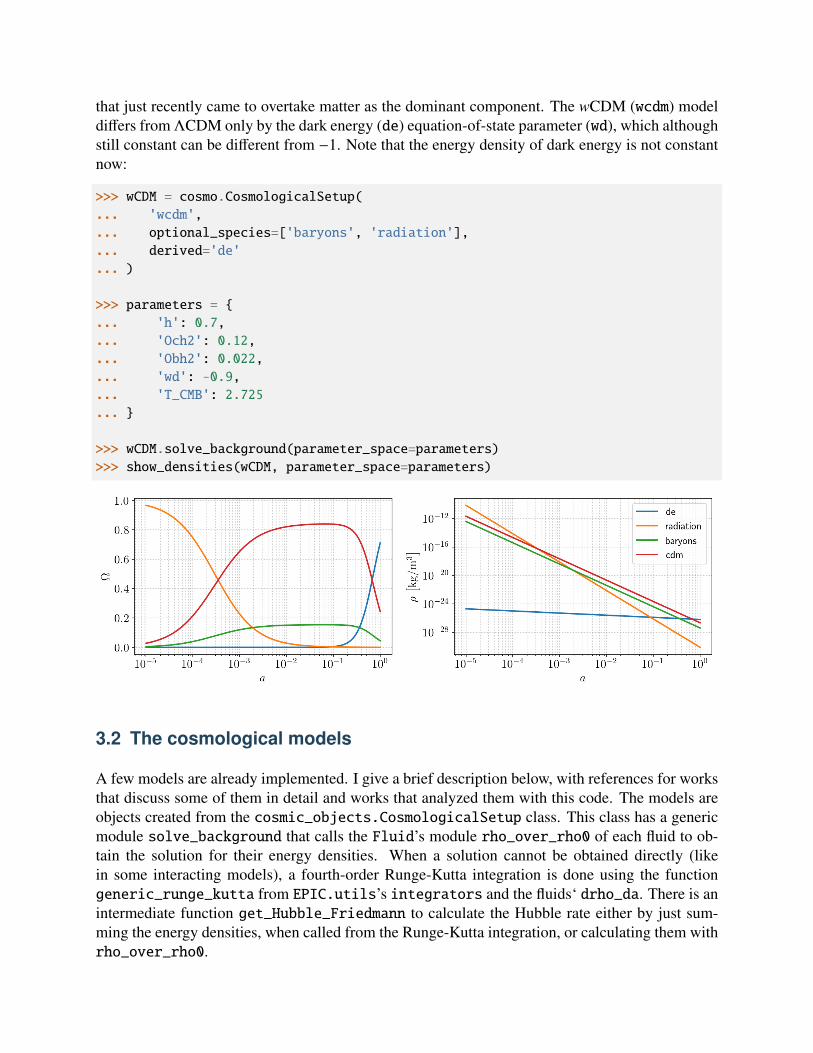
that just recently came to overtake matter as the dominant component. The wCDM (wcdm) modeldiffers from ΛCDM only by the dark energy (de) equation-of-state parameter (wd), which althoughstill constant can be different from −1. Note that the energy density of dark energy is not constantnow:

>>> wCDM = cosmo.CosmologicalSetup(... 'wcdm',... optional_species=['baryons', 'radiation'],... derived='de'... )

>>> parameters = ... 'h': 0.7,... 'Och2': 0.12,... 'Obh2': 0.022,... 'wd': -0.9,... 'T_CMB': 2.725...

>>> wCDM.solve_background(parameter_space=parameters)>>> show_densities(wCDM, parameter_space=parameters)

3.2 The cosmological models

A few models are already implemented. I give a brief description below, with references for worksthat discuss some of them in detail and works that analyzed them with this code. The models areobjects created from the cosmic_objects.CosmologicalSetup class. This class has a genericmodule solve_background that calls the Fluid’s module rho_over_rho0 of each fluid to ob-tain the solution for their energy densities. When a solution cannot be obtained directly (likein some interacting models), a fourth-order Runge-Kutta integration is done using the functiongeneric_runge_kutta from EPIC.utils’s integrators and the fluids‘ drho_da. There is anintermediate function get_Hubble_Friedmann to calculate the Hubble rate either by just sum-ming the energy densities, when called from the Runge-Kutta integration, or calculating them withrho_over_rho0.

Some new models can be introduced in the code just by editing the model_recipes.ini,available_species.ini and (optionally) default_parameter_values.ini configurationfiles, without needing to rebuild and install the EPIC’s package. The format of the configura-tion .ini files is pretty straightforward and the containing information can serve as a guide forwhat needs to be defined.

The ΛCDM model

When baryons and radiation are included, the solution to this cosmology will require values for theparameters Ωc0, Ωb0, TCMB, H0, or h, Ωc0h2, Ωb0h2, TCMB, and will find ΩΛ = 1− (Ωc0 + Ωb0 + Ωr0)or ΩΛh2 = h2−

(Ωc0h2 + Ωb0h2 + Ωr0h2

)if physical.1 The radiation density parameter Ωr0 is cal-

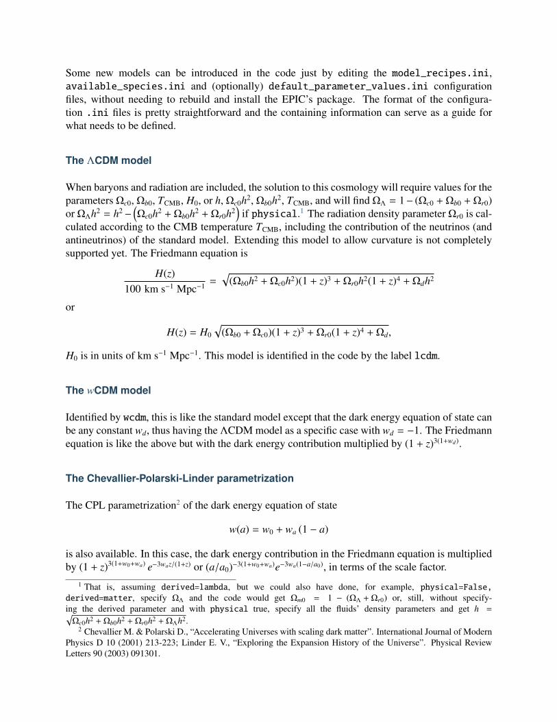
culated according to the CMB temperature TCMB, including the contribution of the neutrinos (andantineutrinos) of the standard model. Extending this model to allow curvature is not completelysupported yet. The Friedmann equation is

H(z)100 km s−1 Mpc−1 =

√(Ωb0h2 + Ωc0h2)(1 + z)3 + Ωr0h2(1 + z)4 + Ωdh2

or

H(z) = H0

√(Ωb0 + Ωc0)(1 + z)3 + Ωr0(1 + z)4 + Ωd,

H0 is in units of km s−1 Mpc−1. This model is identified in the code by the label lcdm.

The wCDM model

Identified by wcdm, this is like the standard model except that the dark energy equation of state canbe any constant wd, thus having the ΛCDM model as a specific case with wd = −1. The Friedmannequation is like the above but with the dark energy contribution multiplied by (1 + z)3(1+wd).

The Chevallier-Polarski-Linder parametrization

The CPL parametrization2 of the dark energy equation of state

w(a) = w0 + wa (1 − a)

is also available. In this case, the dark energy contribution in the Friedmann equation is multipliedby (1 + z)3(1+w0+wa) e−3waz/(1+z) or (a/a0)−3(1+w0+wa)e−3wa(1−a/a0), in terms of the scale factor.

1 That is, assuming derived=lambda, but we could also have done, for example, physical=False,derived=matter, specify ΩΛ and the code would get Ωm0 = 1 − (ΩΛ + Ωr0) or, still, without specify-ing the derived parameter and with physical true, specify all the fluids’ density parameters and get h =√

Ωc0h2 + Ωb0h2 + Ωr0h2 + ΩΛh2.2 Chevallier M. & Polarski D., “Accelerating Universes with scaling dark matter”. International Journal of Modern

Physics D 10 (2001) 213-223; Linder E. V., “Exploring the Expansion History of the Universe”. Physical ReviewLetters 90 (2003) 091301.

The Barboza-Alcaniz parametrization

The Barboza-Alcaniz dark energy equation of state parametrization3

w(z) = w0 + w1z (1 + z)1 + z2

is implemented. This models gives a dark energy contribution in the Friedmann equation that ismultiplied by the term x3(1+w0)

(x2 − 2x + 2

)−3w1/2, where x ≡ a0/a.

Interacting Dark Energy models

A comprehensive review of models that consider a possible interaction between dark energy anddark matter is given by Wang et al. (2016)4. In interacting models, the individual conservationequations of the two dark fluids are violated, although still preserving the total energy conservation:

ρc + 3Hρc = Qρd + 3H(1 + wd)ρd = −Q.

The shape of Q is what characterizes each model. Common forms are proportional to ρc, to ρd

(both supported) or to some combination of both (not supported in this version).

To create an instance of a coupled model (cde) with Q ∝ ρc, use:

>>> from EPIC.cosmology import cosmic_objects as cosmo

>>> CDE = cosmo.CosmologicalSetup(... 'cde',... interaction_setup=... 'species': ['idm', 'ide'],... 'parameter': 'idm': 'xi',... 'propto_other': 'ide': 'idm',... 'sign': 'idm':1, 'ide':-1,... ,... physical=False,... derived='ide'... )

The mandatory species are idm and ide. You can add baryons in the optional_species listkeyword argument, but note that matter is not available as a combined species for this model typesince dark matter is interacting with another fluid while baryons are not. What is new here is theinteraction_setup dictionary. This is where we tell the code which species are interacting(at the moment only an energy exchange within a pair is supported), to which of them (idm) we

3 Barboza E. M. & Alcaniz J. S., “A parametric model for dark energy”. Physics Letters B 666 (2008) 415-419.4 Wang B., Abdalla E., Atrio-Barandela F., Pavón D., “Dark matter and dark energy interactions: theoretial chal-

lenges, cosmological implications and observational signatures”. Reports on Progress in Physics 79 (2016) 096901.

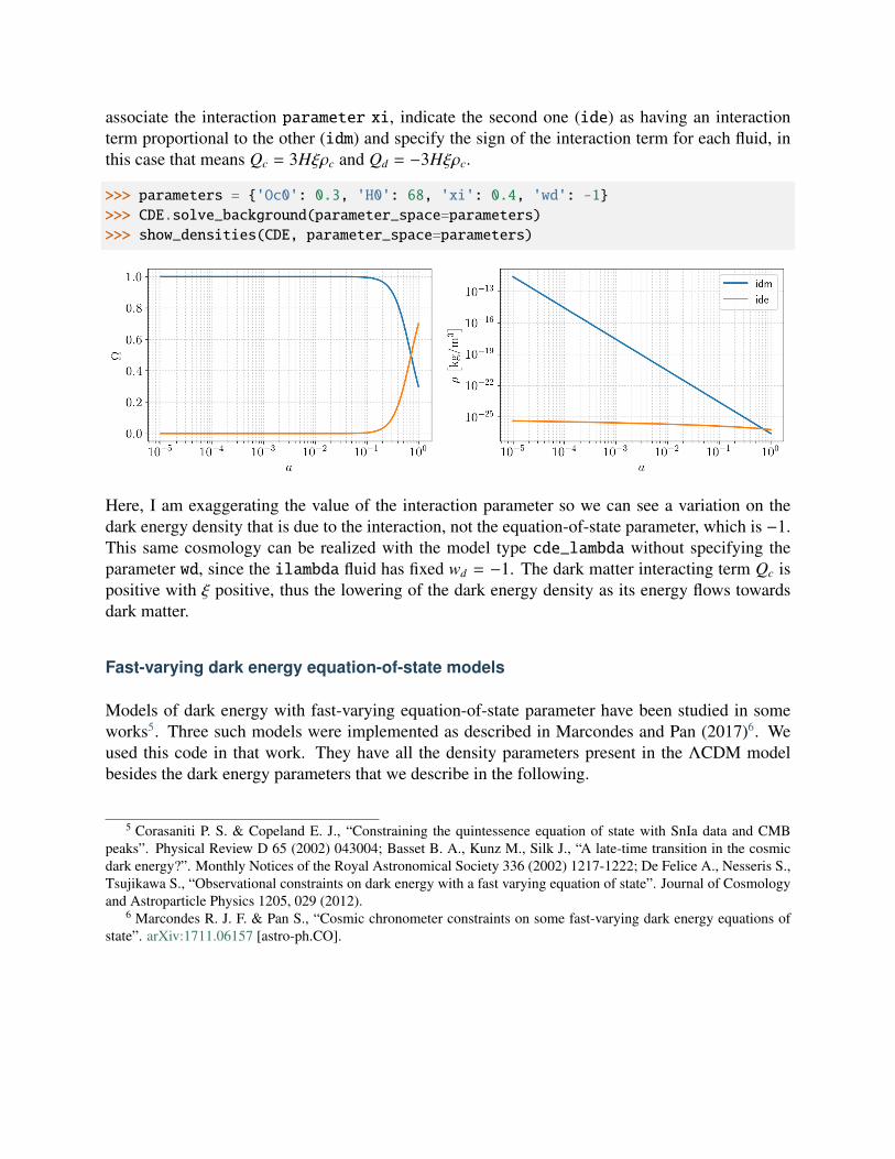
associate the interaction parameter xi, indicate the second one (ide) as having an interactionterm proportional to the other (idm) and specify the sign of the interaction term for each fluid, inthis case that means Qc = 3Hξρc and Qd = −3Hξρc.

>>> parameters = 'Oc0': 0.3, 'H0': 68, 'xi': 0.4, 'wd': -1>>> CDE.solve_background(parameter_space=parameters)>>> show_densities(CDE, parameter_space=parameters)

Here, I am exaggerating the value of the interaction parameter so we can see a variation on thedark energy density that is due to the interaction, not the equation-of-state parameter, which is −1.This same cosmology can be realized with the model type cde_lambda without specifying theparameter wd, since the ilambda fluid has fixed wd = −1. The dark matter interacting term Qc ispositive with ξ positive, thus the lowering of the dark energy density as its energy flows towardsdark matter.

Fast-varying dark energy equation-of-state models

Models of dark energy with fast-varying equation-of-state parameter have been studied in someworks5. Three such models were implemented as described in Marcondes and Pan (2017)6. Weused this code in that work. They have all the density parameters present in the ΛCDM modelbesides the dark energy parameters that we describe in the following.

5 Corasaniti P. S. & Copeland E. J., “Constraining the quintessence equation of state with SnIa data and CMBpeaks”. Physical Review D 65 (2002) 043004; Basset B. A., Kunz M., Silk J., “A late-time transition in the cosmicdark energy?”. Monthly Notices of the Royal Astronomical Society 336 (2002) 1217-1222; De Felice A., Nesseris S.,Tsujikawa S., “Observational constraints on dark energy with a fast varying equation of state”. Journal of Cosmologyand Astroparticle Physics 1205, 029 (2012).

6 Marcondes R. J. F. & Pan S., “Cosmic chronometer constraints on some fast-varying dark energy equations ofstate”. arXiv:1711.06157 [astro-ph.CO].

Model 1

This model fv1 has the free parameters wp, w f , at and τ characterizing the equation of state

wd(a) = w f +wp − w f

1 + (a/at)1/τ .

wp and w f are the asymptotic values of wd in the past (a → 0) and in the future (a → ∞), respec-tively; at is the scale factor at the transition epoch and τ is the transition width. The Friedmannequation is

H(a)2

H20

=Ωr0

a4 +Ωm0

a3 +Ωd0

a3(1+wp) f1(a),

where

f1(a) =

⎛⎜⎜⎜⎜⎝a1/τ + a1/τt

1 + a1/τt

⎞⎟⎟⎟⎟⎠3τ(wp−w f )

.

Model 2

This model fv2 alters the previous model to allow the dark energy to feature an extremum valueof the equation of state:

wd(a) = wp + (w0 − wp) a1 − (a/at)1/τ

1 − (1/at)1/τ ,

where w0 is the current value of the equation of state and the other parameters have the interpreta-tion as in the previous model. The Friedmann equation is

H(a)2

H20

=Ωr0

a4 +Ωm0

a3 +Ωd0

a3(1+wp) e f2(a),

with

f2(a) = 3(w0 − wp)1 + (1 − a−1/τ

t )τ + a[

(a/at)1/τ − 1τ − 1

](1 + τ)(1 − a−1/τ

t ).

Model 3

Finally, we have a third model fv3 with the same parameters as in Model 2 but with equation ofstate

wd(a) = wp + (w0 − wp) a1/τ 1 − (a/at)1/τ

1 − (1/at)1/τ .

It has a Friedmann equation identical to Model 2’s except that f2(a) is replaced by

f3(a) = 3(w0 − wp)τ2 − a−1/τ

t + a1/τt[(a/at)1/τ − 2

]2(1 − a−1/τ

t) .

3.3 The datasets

Observations available for comparison with model predictions are registered in the EPIC/cosmology/observational_data/available_observables.ini. They are separated in sec-tions (Hz, H0, SNeIa, BAO and CMB), which contain the name of the CosmologicalSetup’s mod-ule for the observable theoretical calculation (predicting_function_name). Each dataset goesbelow one of the sections, with the folder or text file containing the data indicated. The path isrelative to the EPIC/cosmology/observational_data/ folder. If the folder name is the sameas the observable label it can be ommited. Besides, the Dataset subclasses are defined at the be-ginning of the .ini file. Each of these classes has its own methods for initialization and likelihoodevaluation.

We choose the datasets by passing a dictionary with observables as keys and datasets as values tothe function choose_from_datasets from observations in EPIC.cosmology:

>>> from EPIC.cosmology import observations

>>> datasets = observations.choose_from_datasets(... 'Hz': 'cosmic_chronometers',... 'H0': 'HST_local_H0',... 'SNeIa': 'JLA_simplified',... 'BAO': [... '6dF+SDSS_MGS', # z = 0.122... 'SDSS_BOSS_CMASS', # z = 0.57... 'SDSS_BOSS_LOWZ', # z = 0.32, 0.57... 'SDSS_BOSS_QuasarLyman', # z = 2.36... 'SDSS_BOSS_consensus', # z = [0.38, 0.51, 0.61]... 'SDSS_BOSS_Lyalpha-Forests', # z = 2.33... #'WiggleZ', # z = [0.44, 0.6, 0.73]... ],... 'CMB': 'Planck2015_distances_LCDM',... )

The WiggleZ dataset is available but is commented out because it is correlated with the SDSSdatasets and thus not supposed to be used together with them. Refer to the papers published bythe authors of the observations for details. Other incompatible combinations are defined in theconflicting_dataset_pairs.txt file in EPIC/cosmology/observational_data/. Thecode will check for these conflicts prior to proceeding with an analysis. The returned flatteneddictionary of Dataset objects will later be passed to a MCMC analysis. Now I describe briefly thedatasets made available by the community.

Type Ia supernovae

Two types of analyses can be made with the JLA catalogue. One can either use the full likelihood(JLA_full) or a simplified version based on 30 redshift bins (JLA_simplified). Here we areusing the binned data consisting of distance modulus estimates at 31 points (defining 30 bins of

redshift). If you want to use the full dataset (which makes the analysis much slower since it involvesthree more nuisance parameters and requires the program to invert a 740 by 740 matrix at everyiteration for the calculation of the JLA likelihood), you need to download the covariance matrixdata (covmat_v6.tgz) from http://supernovae.in2p3.fr/sdss_snls_jla/ReadMe.html. The covmatfolder must be extracted to the jla_likelihood_v6 folder. This is not included in EPIC becausethe data files are too big.

Either way, the data location is the same data folder jla_likelihood_v6. Note that thebinned dataset introduces one nuisance parameter M, representing an overall shift in the abso-lute magnitudes, and the full dataset introduces four nuisance parameters related to the light-curveparametrization. See Betoule et al. (2014)1 for more details.

CMB distance priors

Constraining models with temperature or polarization anisotropy amplitudes is not currently im-plemented. However, you can include the CMB distance priors from Planck2015.2 The datasetsconsist of an acoustic scale lA, a shift parameter R and the physical density of baryons Ωb0h2. Youcan choose between the data for ΛCDM and wCDM with either Planck2015_distances_LCDMor Planck2015_distances_wCDM. Planck2015_distances_LCDM+Omega_k is also availablefor When curvature is supported.

BAO data

Measurements of the baryon acoustic scales from the Six Degree Field Galaxy Survey (6dF) com-bined with the most recent data releases of Sloan Digital Sky Survey (SDSS-MGS),3 the LOWZand CMASS galaxy samples of the Baryon Oscillation Spectroscopic Survey (BOSS-LOWZ andBOSS-CMASS),4 data from the Quasar-Lyman α cross-correlation,5 the distribution of the Lymanα forest in BOSS6 and from the WiggleZ Dark Energy Survey7 are available in the BAO folder, aswell as the latest consensus from the completed SDSS-III BOSS survey.8 The observable is based

1 Betoule M. et al. “Improved cosmological constraints from a joint analysis of the SDSS-II and SNLS supernovasamples”. Astronomy & Astrophysics 568, A22 (2014).

2 Huang Q.-G., Wang K. & Wang S. “Distance priors from Planck 2015 data”. Journal of Cosmology and As-troparticle Physics 12 (2015) 022.

3 Carter P. et al. “Low Redshift Baryon Acoustic Oscillation Measurement from the Reconstructed 6-degree FieldGalaxy Survey”. arXiv:1803.01746v1 [astro-ph.CO].

4 Anderson L. et al. “The clustering of galaxies in the SDSS-III Baryon Oscillation Spectroscopic Survey: measur-ing DA and H at z = 0.57 from the baryon acoustic peak in the Data Release 9 spectroscopic Galaxy sample”. MonthlyNotices of the Royal Astronomical Society 438 (2014) 83-101.

5 Font-Ribera A. et al. “Quasar-Lyman α forest cross-correlation from BOSS DR11: Baryon Acoustic Oscilla-tions”. Journal of Cosmology and Astroparticle Physics 05 (2014) 027.

6 Bautista J. E. et al. “Measurement of baryon acoustic oscillation correlations at z = 2.3 with SDSS DR12 Lyα-Forests”. Astronomy & Astrophysics 603 (2017) A12.

7 Kazin E. A. et al. “The WiggleZ Dark Energy Survey: improved distance measurements to z = 1 with reconstruc-tion of the baryonic acoustic feature”. Monthly Notices of the Royal Astronomical Society 441 (2014) 3524-3542.

8 Alam S. et al. “The clustering of galaxies in the completed SDSS-III Baryon Oscillation Spectroscopic Survey:cosmological analysis of the DR12 galaxy sample”. Monthly Notices of the Royal Astronomical Society 470 (2017)

on the value of the characteristic ratio rs(zd)/DV(z) between the sound horizon rs at decouplingtime (zd) and the effective BAO distance DV , or some variation of this. The respective referencesare given in the headers of the data files.

H(z) data

These are the cosmic chronometer data. 30 measurements of the Hubble expansion rate H(z) atredshifts between 0 and 2.9 The values of redshift, H and the uncertainties are given in the fileHz/Hz_Moresco_et_al_2016.txt.

H0 data

The 2.4% precision local measure10 of H0 is present in H0/local_H0_Riess_et_al_2016.txt.

3.4 The calculator GUI

Calculations like the ones presented in the previous section can also be executed from a GraphicalUser Interface (GUI). This makes it easy for the unexperienced user, although learning to useEPIC with the interactive Python interpreter is encouraged. The command to launch the GUI isgui. However, starting with version 1.3, you can omit this command. Opening the GUI is thedefault behavior of the script. From the terminal, activate your environment and run:

$ epic.py

This is equivalent to epic.py gui (but python epic.py might be needed depending on yoursystem). Optionally, you can also use $ python -W ignore epic.py gui to ignore somewarnings that will be issued by matplotlib (note that this will actually omit all warnings). Thefollowing screen will appear:

2617-2652.9 Moresco M. et al. “A 6% measurement of the Hubble parameter at z ∼ 0.45: direct evidence of the epoch of

cosmic re-acceleration”. Journal of Cosmology and Astroparticle Physics 05 (2016) 014.10 Riess A. G. et al. “A 2.4% determination of the local value of the Hubble constant”. The Astrophysical Journal

826 (2016) 56.

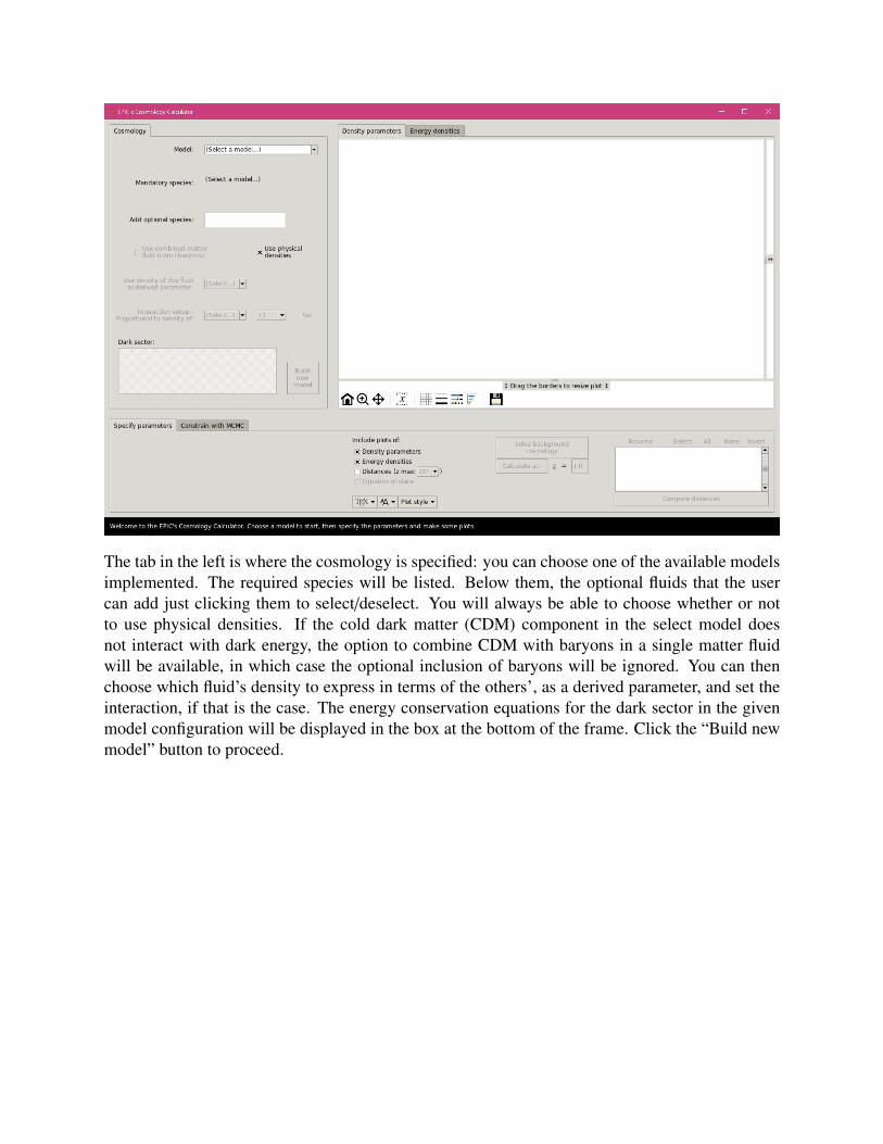
The tab in the left is where the cosmology is specified: you can choose one of the available modelsimplemented. The required species will be listed. Below them, the optional fluids that the usercan add just clicking them to select/deselect. You will always be able to choose whether or notto use physical densities. If the cold dark matter (CDM) component in the select model doesnot interact with dark energy, the option to combine CDM with baryons in a single matter fluidwill be available, in which case the optional inclusion of baryons will be ignored. You can thenchoose which fluid’s density to express in terms of the others’, as a derived parameter, and set theinteraction, if that is the case. The energy conservation equations for the dark sector in the givenmodel configuration will be displayed in the box at the bottom of the frame. Click the “Build newmodel” button to proceed.

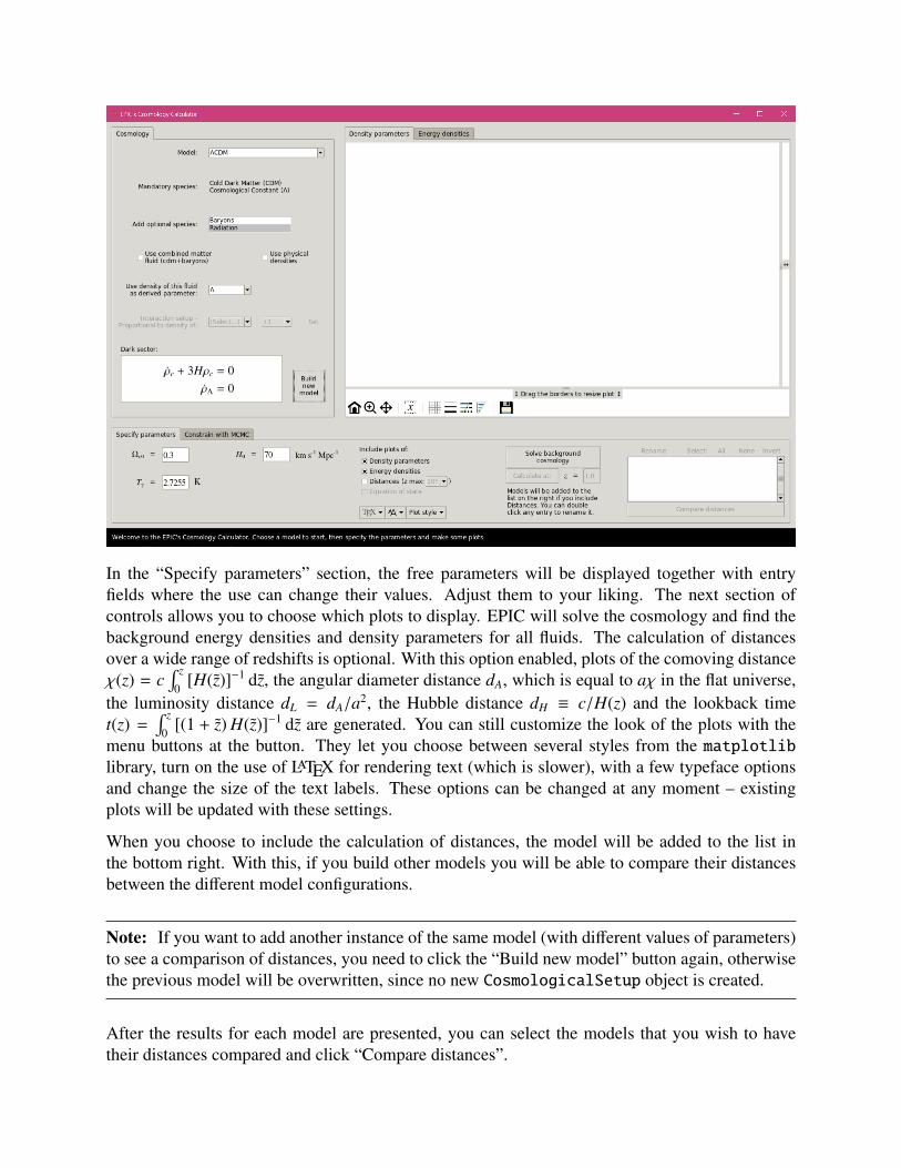
In the “Specify parameters” section, the free parameters will be displayed together with entryfields where the use can change their values. Adjust them to your liking. The next section ofcontrols allows you to choose which plots to display. EPIC will solve the cosmology and find thebackground energy densities and density parameters for all fluids. The calculation of distancesover a wide range of redshifts is optional. With this option enabled, plots of the comoving distanceχ(z) = c

∫ z

0[H(z)]−1 dz, the angular diameter distance dA, which is equal to aχ in the flat universe,

the luminosity distance dL = dA/a2, the Hubble distance dH ≡ c/H(z) and the lookback timet(z) =

∫ z

0[(1 + z) H(z)]−1 dz are generated. You can still customize the look of the plots with the

menu buttons at the button. They let you choose between several styles from the matplotliblibrary, turn on the use of LaTEX for rendering text (which is slower), with a few typeface optionsand change the size of the text labels. These options can be changed at any moment – existingplots will be updated with these settings.

When you choose to include the calculation of distances, the model will be added to the list inthe bottom right. With this, if you build other models you will be able to compare their distancesbetween the different model configurations.

Note: If you want to add another instance of the same model (with different values of parameters)to see a comparison of distances, you need to click the “Build new model” button again, otherwisethe previous model will be overwritten, since no new CosmologicalSetup object is created.

After the results for each model are presented, you can select the models that you wish to havetheir distances compared and click “Compare distances”.

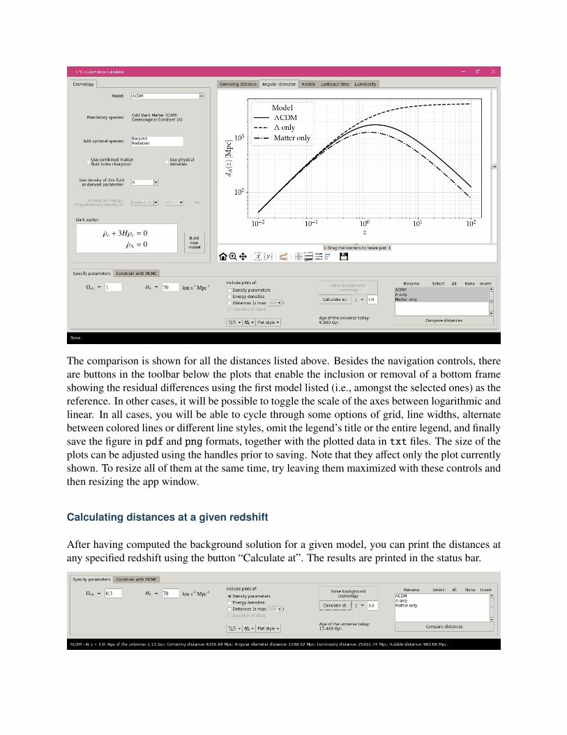
The comparison is shown for all the distances listed above. Besides the navigation controls, thereare buttons in the toolbar below the plots that enable the inclusion or removal of a bottom frameshowing the residual differences using the first model listed (i.e., amongst the selected ones) as thereference. In other cases, it will be possible to toggle the scale of the axes between logarithmic andlinear. In all cases, you will be able to cycle through some options of grid, line widths, alternatebetween colored lines or different line styles, omit the legend’s title or the entire legend, and finallysave the figure in pdf and png formats, together with the plotted data in txt files. The size of theplots can be adjusted using the handles prior to saving. Note that they affect only the plot currentlyshown. To resize all of them at the same time, try leaving them maximized with these controls andthen resizing the app window.

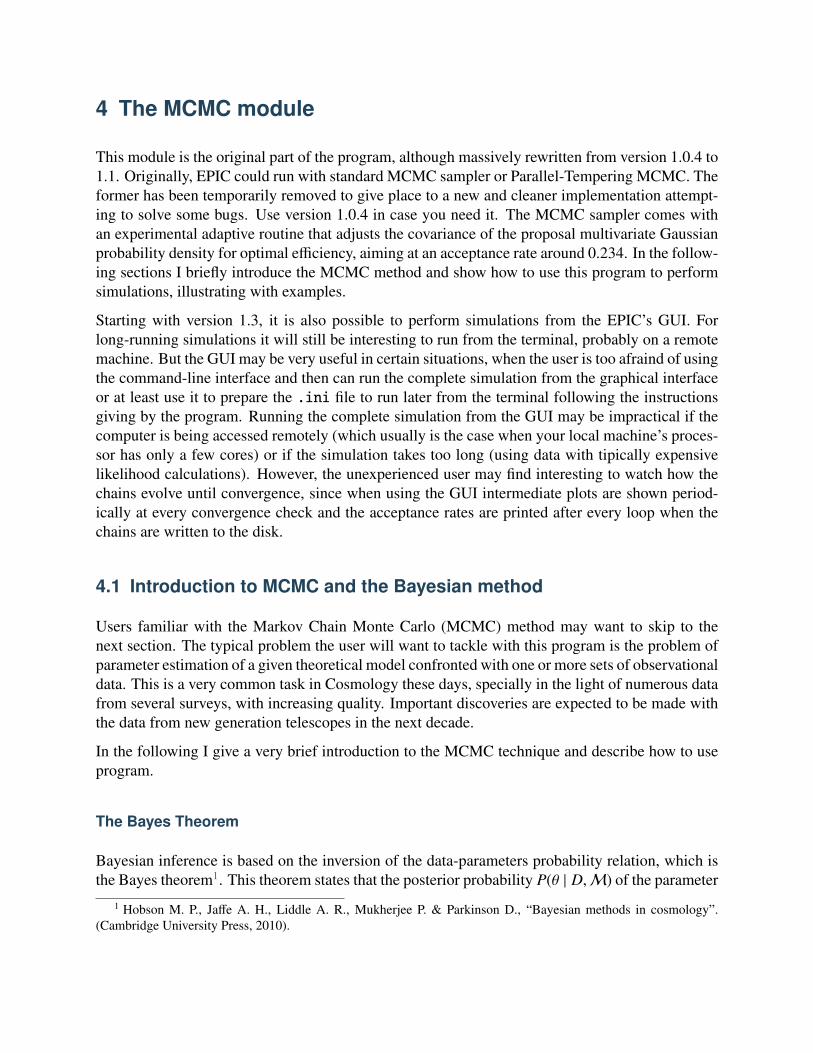
Calculating distances at a given redshift

After having computed the background solution for a given model, you can print the distances atany specified redshift using the button “Calculate at”. The results are printed in the status bar.

4 The MCMC module

This module is the original part of the program, although massively rewritten from version 1.0.4 to1.1. Originally, EPIC could run with standard MCMC sampler or Parallel-Tempering MCMC. Theformer has been temporarily removed to give place to a new and cleaner implementation attempt-ing to solve some bugs. Use version 1.0.4 in case you need it. The MCMC sampler comes withan experimental adaptive routine that adjusts the covariance of the proposal multivariate Gaussianprobability density for optimal efficiency, aiming at an acceptance rate around 0.234. In the follow-ing sections I briefly introduce the MCMC method and show how to use this program to performsimulations, illustrating with examples.

Starting with version 1.3, it is also possible to perform simulations from the EPIC’s GUI. Forlong-running simulations it will still be interesting to run from the terminal, probably on a remotemachine. But the GUI may be very useful in certain situations, when the user is too afraind of usingthe command-line interface and then can run the complete simulation from the graphical interfaceor at least use it to prepare the .ini file to run later from the terminal following the instructionsgiving by the program. Running the complete simulation from the GUI may be impractical if thecomputer is being accessed remotely (which usually is the case when your local machine’s proces-sor has only a few cores) or if the simulation takes too long (using data with tipically expensivelikelihood calculations). However, the unexperienced user may find interesting to watch how thechains evolve until convergence, since when using the GUI intermediate plots are shown period-ically at every convergence check and the acceptance rates are printed after every loop when thechains are written to the disk.

4.1 Introduction to MCMC and the Bayesian method

Users familiar with the Markov Chain Monte Carlo (MCMC) method may want to skip to thenext section. The typical problem the user will want to tackle with this program is the problem ofparameter estimation of a given theoretical model confronted with one or more sets of observationaldata. This is a very common task in Cosmology these days, specially in the light of numerous datafrom several surveys, with increasing quality. Important discoveries are expected to be made withthe data from new generation telescopes in the next decade.

In the following I give a very brief introduction to the MCMC technique and describe how to useprogram.

The Bayes Theorem

Bayesian inference is based on the inversion of the data-parameters probability relation, which isthe Bayes theorem1. This theorem states that the posterior probability P(θ | D,ℳ) of the parameter

1 Hobson M. P., Jaffe A. H., Liddle A. R., Mukherjee P. & Parkinson D., “Bayesian methods in cosmology”.(Cambridge University Press, 2010).

set θ given the data D and other information from the modelℳ can be given by

P(θ | D,ℳ) =ℒ(D | θ,ℳ) π(θ | ℳ)

P(D,ℳ),

where ℒ(D | θ,ℳ) is the likelihood of the data given the model parameters, π(θ | ℳ) is the priorprobability, containing any information known a priori about the distribution of the parameters, andP(D,ℳ) is the marginal likelihood, also popularly known as the evidence, giving the normalizationof the posterior probability. The evidence is not required for the parameter inference but is essentialin problems of selection model, when comparing two or more different models to see which of themis favored by the data.

Direct evaluation of P(θ | D,ℳ) is generally a difficult integration in a multiparameter space thatwe do not know how to perform. Usually we do know how to compute the likelihood ℒ(D | θ,ℳ)that is assigned to the experiment (most commonly a distribution that is Gaussian on the data orthe parameters), thus the use of the Bayes theorem to give the posterior probability. Flat priors arecommonly assumed, which makes the computation of the right-hand side of the equation abovetrivial. Remember that the evidence is a normalization constant not necessary for us to learn aboutthe most likely values of the parameters.

The Metropolis-Hastings sampler

The MCMC method shifts the problem of calculating the unknown posterior probability distribu-tion in the entire space, which can be extremly expensive for models with large number of param-eters, to the problem of sampling from the posterior distribution. This is possible, for example, bygrowing a Markov chain with new states generated by the Metropolis sampler2.

The Markov chain has the property that every new state depends on its current state, and only onthis current state. Dependence on more previous states or on some statistics involving all statesis not allowed. That can be done and can even also be useful for purposes like ours, but then thechain can not be called Markovian.

The standard MCMC consists of generating a random state y according to a proposal probabilityQ(· | xt) given the current state xt at time t. Then a random number u is drawn from a uniformdistribution between 0 and 1. The new state is accepted if r ≥ u, where

r = min[1,

P(y | D,ℳ)Q(xt | y)P(xt | D,ℳ)Q(y | xt)

].

The fraction is the Metropolis-Hastings ratio. When the proposal function is symmetrical, Q(xt |y)Q(y|xt)

reduces to 1 and the ratio is just the original Metropolis ratio of the posteriors. If the new state isaccepted, we set xt+1 := y, otherwise we repeat the state in the chain by setting xt+1 := xt.

2 Gayer C., “Introduction to Markov Chain Monte Carlo”. in “Handbook of Markov Chain Monte Carlo” http://www.mcmchandbook.net/

The acceptance rate α =number of accepted states

total number of states of a chain should be around 0.234 for optimal effi-ciency3. This can be obtained by tuning the parameters of the function Q. In this implementation,I use a multivariate Gaussian distribution with a diagonal covariance matrix S .

The Parallel Tempering algorithm (removed in this version)

Standard MCMC is powerful and works in most cases but there are some problems where theuser may be better off using some other method. Due to the characteristic behavior of a Markovchain, it is possible (and even likely) that a chain become stuck in a single mode of a multimodaldistribution. If two or more peaks are far away from each other, the proposal function tuned forgood performance in a peak may have difficulty escaping that peak to explore the other, because thejump may be too short. To overcome this inefficiency, a neat variation of MCMC, called ParallelTempering4, favors a better exploration of the entire parameter space in such cases thanks to anarrangement of multiple chains that are run in parallel, each one with a different ‘’temperature”T . The posterior is calculated as ℒβπ, with β = 1/T . The first chain is the one that correspondsto the real life posterior we are interested in; the other chains, at higher temperatures, will havewider distributions, which makes it easier to jump between peaks, thus exploring more properlythe parameter space. Periodically, a swap of states between neighboring chains is proposed andaccepted or rejected according to a Hastings-like ratio.

4.2 Before starting

In the section The Cosmology calculator we learned how to use EPIC to set up a cosmologicalmodel and load some datasets. The next logical step is to calculate the probability density at agiven point of the parameter space, given that model and according to the chosen data. This can bedone as follows:

>>> import EPIC.cosmology.cosmic_objects as cosmo>>> from EPIC.cosmology import observations>>> from EPIC.utils.statistics import Analysis

>>> lcdm = cosmo.CosmologicalSetup(... 'lcdm', physical=False, derived='lambda'... )

>>> datasets = observations.choose_from_datasets(... 'Hz': 'cosmic_chronometers',... 'H0': 'HST_local_H0',... 'SNeIa': 'JLA_simplified',

(continues on next page)

3 Roberts G. O. & Rosenthal J. S., “Optimal scaling for various Metropolis-Hastings algorithms”. Statistical Sci-ence 16 (2001) 351-367.

4 Gregory P. C., “Bayesian logical data analysis for the physical sciences: a comparative approach with Mathemat-ica support”. (Cambridge University Press, 2005).

(continued from previous page)

... )

>>> priors = ... 'Oc0' : [0, 0.5],... 'H0' : [50, 90],... 'M' : [-0.3, 0.3],... >>> analysis = Analysis(datasets, lcdm, priors)>>> analysis.log_posterior(parameter_space='Oc0': 0.3, 'H0': 68, 'M': 0,→chi2=True)(-38.37946644320705, -35.38373416965306)

In this example I am choosing the cosmic chronometers dataset, the Hubble constant local mea-surement and the simplified version of the JLA dataset. The Analysis object is created from thedictionary of datasets, the model and a dictionary of priors in the model parameters (including nui-sance parameters related to the data). The probability density at any point can then be calculatedwith the module log_posterior, which returns the logarithm of the posterior probability densityand the logarithm of the likelihood. Setting the option chi2 to True (It is False by default) makesthe calculation of the likelihood as logℒ = −χ2/2, dropping the usual multiplicative terms fromthe normalized Gaussian likelihood. When false, the results include the contribution of the factors1/√

2πσi or the factor 1/√

2π|C|. These are constant in most cases, making no difference to theanalysis, but in other cases, depending on the data set, the covariance matrix C can depend onnuisance parameters and thus vary at each point.

Now that we know how to calculate the posterior probability at a given point, we can perform aMonte Carlo Markov Chain simulation to assess the confidence regions of the model parameters.The main script epic.py accomplishes this making use of the objects and modules here presented.

The configuration of the analysis (choice of model, datasets, priors, etc) is defined in a .iniconfiguration file that the program reads. The program creates a folder in the working directorywith the same name of this .ini file, if it does not already exist. Another folder is created with thedate and time for the output of each run of the code, but you can always continue a previous runfrom where it stopped, just giving the folder name instead of the .ini file. The script is stored inthe EPIC source folder, where the .ini files should also be placed. The default working directoryis the EPIC’s parent directory, i.e., the epic repository folder.

Changing the default working directory

By default, the folders with the name of the .ini files are created at the repository root level. Butthe chains can get very long and you might want to have them stored in a different drive. In orderto set a new default location for all the new files, run:

$ python define_altdir.py

This will ask for the path of the folder where you want to save all the output of the program and

keep this information in a file altdir.txt. If you want to revert this change you can delete thealtdir.txt file or run again the command above and leave the answer empty when prompted.To change this directory temporarily you can use the argument --alt-dir when running the mainscript.

The structure of the .ini file

Let us work with an example, with a simple flat ΛCDM model. Suppose we want to constrain itsparameters with H(z), supernovae data, CMB shift parameters and BAO data. The model parame-ters are the reduced Hubble constant h, the present-day values of the physical density parametersof dark matter Ωc0h2, baryons Ωb0h2 and radiation Ωr0h2. We will not consider perturbations, weare only constraining the parameters at the background level. Since we are using supernovae datawe must include a nuisance parameter M, which represents a shift in the absolute magnitudes ofthe supernovae. Use of the full JLA catalogue requires the inclusion of the nuisance parametersα, β and ∆M from the light-curve fit. The first section of .ini is required to specify the type ofthe model, whether to use physical density parameters or not, and which species has the densityparameter derived from the others (e. g. from the flatness condition):

[model]type = lcdmphysical = yesoptional species = ['baryons', 'radiation']derived = lambda

The lcdm model will always have the two species cdm and lambda. We are including the op-tional baryonic fluid and radiation, which being a combined species replaces photons andneutrinos. The configurations and options available for each model are registered in the EPIC/cosmology/model_recipes.ini file. This section can still received the interaction setupdictionary to set the configuration of an interacting dark sector model. Details on this are given inthe previous section Interacting Dark Energy models.

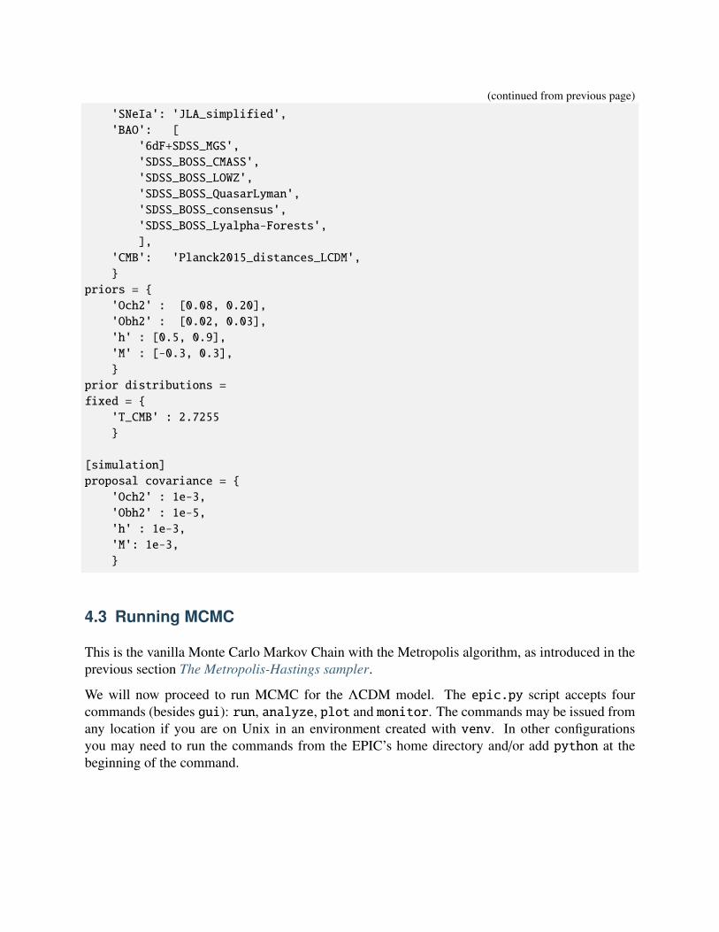
The second section defines the analysis: a label, datasets and specifications about the priors rangesand distributions. The optional property prior distributions can receive a dictionary witheither Flat or Gaussian for each parameter. When not specified, the code will assume flat priorsby default and interpret the list of two numbers as an interval prior range. When Gaussian, thesenumbers are interpreted as the parameters µ and σ of the Gaussian distribution. In the simulationsection, we specify the parameters of the diagonal covariance matrix to be used with the proposalprobability distribution in the sampler. Values comparable to the expected standard deviation ofthe parameter distributions are recommended.

[analysis]label = $H(z)$ + $H_0$ + SNeIa + BAO + CMBdatasets =

'Hz': 'cosmic_chronometers','H0': 'HST_local_H0',

(continues on next page)

(continued from previous page)

'SNeIa': 'JLA_simplified','BAO': [

'6dF+SDSS_MGS','SDSS_BOSS_CMASS','SDSS_BOSS_LOWZ','SDSS_BOSS_QuasarLyman','SDSS_BOSS_consensus','SDSS_BOSS_Lyalpha-Forests',],

'CMB': 'Planck2015_distances_LCDM',

priors = 'Och2' : [0.08, 0.20],'Obh2' : [0.02, 0.03],'h' : [0.5, 0.9],'M' : [-0.3, 0.3],

prior distributions =fixed =

'T_CMB' : 2.7255

[simulation]proposal covariance =

'Och2' : 1e-3,'Obh2' : 1e-5,'h' : 1e-3,'M': 1e-3,

4.3 Running MCMC

This is the vanilla Monte Carlo Markov Chain with the Metropolis algorithm, as introduced in theprevious section The Metropolis-Hastings sampler.

We will now proceed to run MCMC for the ΛCDM model. The epic.py script accepts fourcommands (besides gui): run, analyze, plot and monitor. The commands may be issued fromany location if you are on Unix in an environment created with venv. In other configurationsyou may need to run the commands from the EPIC’s home directory and/or add python at thebeginning of the command.

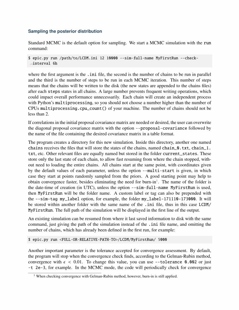
Sampling the posterior distribution

Standard MCMC is the default option for sampling. We start a MCMC simulation with the runcommand:

$ epic.py run /path/to/LCDM.ini 12 10000 --sim-full-name MyFirstRun --check-→interval 6h

where the first argument is the .ini file, the second is the number of chains to be run in paralleland the third is the number of steps to be run in each MCMC iteration. This number of stepsmeans that the chains will be written to the disk (the new states are appended to the chains files)after each steps states in all chains. A large number prevents frequent writing operations, whichcould impact overall performance unnecessarily. Each chain will create an independent processwith Python’s multiprocessing, so you should not choose a number higher than the number ofCPUs multiprocessing.cpu_count() of your machine. The number of chains should not beless than 2.

If correlations in the initial proposal covariance matrix are needed or desired, the user can overwritethe diagonal proposal covariance matrix with the option --proposal-covariance followed bythe name of the file containing the desired covariance matrix in a table format.

The program creates a directory for this new simulation. Inside this directory, another one namedchains receives the files that will store the states of the chains, named chain_0.txt, chain_1.txt, etc. Other relevant files are equally named but stored in the folder current_states. Thesestore only the last state of each chain, to allow fast resuming from where the chain stopped, with-out need to loading the entire chains. All chains start at the same point, with coordinates givenby the default values of each parameter, unless the option --multi-start is given, in whichcase they start at points randomly sampled from the priors. A good starting point may help toobtain convergence faster, besides eliminating the need for burn-in1. The name of the folder isthe date-time of creation (in UTC), unless the option --sim-full-name MyFirstRun is used,then MyFirstRun will be the folder name. A custom label or tag can also be prepended withthe --sim-tag my_label option, for example, the folder my_label-171110-173000. It willbe stored within another folder with the same name of the .ini file, thus in this case LCDM/MyFirstRun. The full path of the simulation will be displayed in the first line of the output.

An existing simulation can be resumed from where it last saved information to disk with the samecommand, just giving the path of the simulation instead of the .ini file name, and omitting thenumber of chains, which has already been defined in the first run, for example:

$ epic.py run <FULL-OR-RELATIVE-PATH-TO>/LCDM/MyFirstRun/ 5000

Another important parameter is the tolerance accepted for convergence assessment. By default,the program will stop when the convergence check finds, according to the Gelman-Rubin method,convergence with ε < 0.01. To change this value, you can use --tolerance 0.002 or just-t 2e-3, for example. In the MCMC mode, the code will periodically check for convergence

1 When checking convergence with Gelman-Rubin method, however, burn-in is still applied.

according to the Gelman-Rubin method (by default it is done every two hours but can be specifieddifferently as --check-interval 12h or -c 45min in the arguments, for example. This doesnot need to (and should not) be a small time interval, but the option to specify this time in minutesor even in seconds (30sec) is implemented and available for testing purposes.

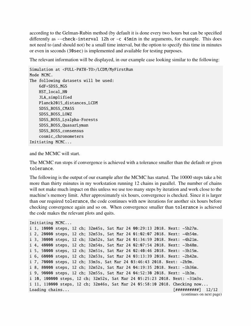
The relevant information will be displayed, in our example case looking similar to the following:

Simulation at <FULL-PATH-TO>/LCDM/MyFirstRunMode MCMC.The following datasets will be used:

6dF+SDSS_MGSHST_local_H0JLA_simplifiedPlanck2015_distances_LCDMSDSS_BOSS_CMASSSDSS_BOSS_LOWZSDSS_BOSS_Lyalpha-ForestsSDSS_BOSS_QuasarLymanSDSS_BOSS_consensuscosmic_chronometers

Initiating MCMC...

and the MCMC will start.

The MCMC run stops if convergence is achieved with a tolerance smaller than the default or giventolerance.

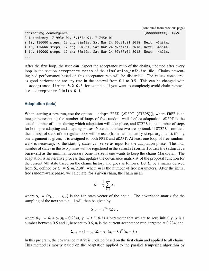
The following is the output of our example after the MCMC has started. The 10000 steps take a bitmore than thirty minutes in my workstation running 12 chains in parallel. The number of chainswill not make much impact on this unless we use too many steps by iteration and work close to themachine’s memory limit. After approximately six hours, convergence is checked. Since it is largerthan our required tolerance, the code continues with new iterations for another six hours beforechecking convergence again and so on. When convergence smaller than tolerance is achievedthe code makes the relevant plots and quits.

Initiating MCMC...i 1, 10000 steps, 12 ch; 32m45s, Sat Mar 24 00:29:13 2018. Next: ~5h27m.i 2, 20000 steps, 12 ch; 32m53s, Sat Mar 24 01:02:07 2018. Next: ~4h54m.i 3, 30000 steps, 12 ch; 32m52s, Sat Mar 24 01:34:59 2018. Next: ~4h21m.i 4, 40000 steps, 12 ch; 32m54s, Sat Mar 24 02:07:54 2018. Next: ~3h48m.i 5, 50000 steps, 12 ch; 32m51s, Sat Mar 24 02:40:46 2018. Next: ~3h15m.i 6, 60000 steps, 12 ch; 32m53s, Sat Mar 24 03:13:39 2018. Next: ~2h42m.i 7, 70000 steps, 12 ch; 33m3s, Sat Mar 24 03:46:43 2018. Next: ~2h9m.i 8, 80000 steps, 12 ch; 32m52s, Sat Mar 24 04:19:35 2018. Next: ~1h36m.i 9, 90000 steps, 12 ch; 32m55s, Sat Mar 24 04:52:30 2018. Next: ~1h3m.i 10, 100000 steps, 12 ch; 32m52s, Sat Mar 24 05:25:23 2018. Next: ~31m3s.i 11, 110000 steps, 12 ch; 32m46s, Sat Mar 24 05:58:10 2018. Checking now...Loading chains... [##########] 12/12

(continues on next page)

(continued from previous page)

Monitoring convergence... [##########] 100%R-1 tendency: 7.993e-01, 8.185e-01, 7.745e-01i 12, 120000 steps, 12 ch; 32m49s, Sat Mar 24 06:31:21 2018. Next: ~5h27m.i 13, 130000 steps, 12 ch; 32m53s, Sat Mar 24 07:04:15 2018. Next: ~4h54m.i 14, 140000 steps, 12 ch; 32m49s, Sat Mar 24 07:37:04 2018. Next: ~4h21m....

After the first loop, the user can inspect the acceptance ratio of the chains, updated after everyloop in the section acceptance rates of the simulation_info.ini file. Chains present-ing bad performance based on this acceptance rate will be discarded. The values consideredas good performance are any rate in the interval from 0.1 to 0.5. This can be changed with--acceptance-limits 0.2 0.5, for example. If you want to completely avoid chain removaluse --acceptance-limits 0 1.

Adaptation (beta)

When starting a new run, use the option --adapt FREE [ADAPT [STEPS]], where FREE is aninteger representing the number of loops of free random-walk before adaptation, ADAPT is theactual number of loops during which adaptation will take place, and STEPS is the number of stepsfor both, pre-adapting and adapting phases. Note that the last two are optional. If STEPS is omitted,the number of steps of the regular loops will be used (from the mandatory steps argument); if onlyone argument is given, it is assigned to both FREE and ADAPT. At least one loop of free random-walk is necessary, so the starting states can serve as input for the adaptation phase. The totalnumber of states in the two phases will be registered in the simulation_info.ini file (adaptiveburn-in) as the minimal necessary burn-in size if one wants to keep the chains Markovian. Theadaptation is an iterative process that updates the covariance matrix St of the proposal function forthe current t-th state based on the chains history and goes as follows. Let Σt be a matrix derivedfrom St, defined by Σt ≡ St m/2.382, where m is the number of free parameters. After the initialfree random-walk phase, we calculate, for a given chain, the chain mean

xt =1t

t∑i=1

xi,

where xi =(x1,i, . . . , xm,i

)is the i-th state vector of the chain. The covariance matrix for the

sampling of the next state t + 1 will then be given by

St+1 = e2θt+1Σt+1,

where θt+1 = θt + γt (ηt − 0.234), γt = t−α, θt is a parameter that we set to zero initially, α is anumber between 0.5 and 1, here set to 0.6, ηt is the current acceptance rate, targeted at 0.234, and

Σt+1 = (1 − γt)Σt + γt (xt − xt)T (xt − xt) .

In this program, the covariance matrix is updated based on the first chain and applied to all chains.This method is mostly based on the adaptation applied to the parallel tempering algorithm by

Łacki & Miasojedow (2016)2. The idea is to obtain a covariance matrix such that the asymptoticacceptance rate is 0.234, considered to be a good value. Note, however, that this feature is in betaand may require some trial and error with the choice of both free random-walk and adaptationphases lengths. It might take too long for the proposal covariance matrix to converge and thesimulation is not guaranteed to keep good acceptance rates with the final matrix obtained after theadaptation phase.

Analyzing the chains

Once convergence is achieved and MCMC is finished, the code reads the chains and extract theinformation for the parameter inference. But this can be done to assess the results while MCMC isstill going on. The distributions are compiled for a nice plot with the command analyze:

$ epic.py analyze <FULL-OR-RELATIVE-PATH-TO>/LCDM/MyFirstRun/

Histograms are generated for the marginalized distributions using 20 bins or any other numbergiven with --bins or -b. At any time one can run this command, optionally with --convergenceor -c to check the state of convergence. By default, this will calculate Rp − 1 for twenty differentsizes (which you can change with --GR-steps) considering the size of the chains to provide anidea of the evolution of the convergence.

Convergence is assessed based on the Gelman-Rubin criterium. I will not enter into details of themethod here, but I refer the reader to the original papers45 for more information. The variation ofthe original method for multivariate distribution is implemented. When using MCMC, all the chainsare checked for convergence and the final resulting distribution which is analyzed and plotted is theconcatenation of all the chains, since they are essentially all the same once they have converged.

Additional options

If for some reason you want to view the results for an intermediate point of the simulation, you cantell the script to --stop-at 18000, everything will be analyzed until that point.

If you want to check the random walk of the chains you can plot the sequences with--plot-sequences. This will make a grid plot containing all the chains and all parameters.Keep in mind that this can take some time and generate a big output file if the chains are verylong. You can contour this problem by thinning the distributions by some factor --thin 10, forexample. This also applies for the calculation of the correlation of the parameters in each chain,enabled with the --correlation-function option.

2 Łacki M. K. & Miasojedow B. “State-dependent swap strategies and automatic reduction of number of tempera-tures in adaptive parallel tempering algorithm”. Statistics and Computing 26, 951–964 (2016).

4 Gelman A & Rubin D. B. “Inference from Iterative Simulation Using Multiple Sequences”. Statistical Science 7(1992) 457-472.

5 Brooks S. P. & Gelman A. “General Methods for Monitoring Convergence of Iterative Simulations”. Journal ofComputational and Graphical Statistics 7 (1998) 434.

We generally represent distributions by their histograms but sometimes we may prefer to exhibitsmooth curves. Although it is possible to choose a higher number of histogram bins, this maynot be sufficient and may required much more data. Much better (although possibly slow whenthere are too many states) are the kernel density estimates (KDE) tuned for Gaussian-like distribu-tions6. To obtain smoothed shapes use --kde. This will compute KDE curves for the marginalizedparameter distributions and also the two-parameter joint posterior probability distributions.

Making the triangle plots

The previous command will also produce the plots automatically (unless supressed with--dont-plot), but you can always redraw everything when you want, maybe you would liketo tweak some colors? Loading the chains again is not necessary since the analysis already savesthe information for the plots anyway. This is done with:

$ epic.py plot <FULL-OR-RELATIVE-PATH-TO>/LCDM/MyFirstRun/

The code will find the longest chain analysis results and plot them. In this plot, you can, forexample, choose the main color with --color m for magenta, or with any other Python colorname, and omit the best-fit point mark with --no-best-fit-marks. You can always use any ofC0, C1, . . . , C9, which refer to the colors in the current style’s palette. The default option is C0.

Plot ranges and eventually necessary factors of power of 10 are automatically handled by thecode, unless you use --no-auto-range and --no-auto-factors or choose your own ranges orpowers of 10 by specifying a dictionary with parameter label as keys and a pair of floats in a listor an integer power of 10 for the entries custom range and custom factors under the sectionanalysis in the .ini file.

If you have used the option --kde previously in the analysis you need to specify it here too tomake the corresponding plots, otherwise the histograms will be drawn.

The 1σ and 2σ confidence levels are shown and are written to the file hist_table.tex (andkde_table.tex if it is the case) inside the folder with the size of the chain preceeded by the lettern. These LaTEX-ready files can be compiled to make a nice table in a PDF file or included in yourpaper as you want. To view and save information for more levels3, use --levels 1 2 3 4 5.

Additional options

You can further tweak your plots and tables. --use-tex will make the program render the plotusing LaTEX, fitting nicely to the rest of your paper. You can plot Gaussian fits together with thehistograms (the Gaussian curve and the two first sigma levels), using --show-gaussian-fits,but probably only for the sake of comparison since this is not usually done in publications. --fmt

6 Kristan M., Leonardis A. and Skocaj D. “Multivariate online kernel density estimation with Gaussian kernels”.Pattern Recognit 44 (2011) 2630-2642.

3 Choice limited up to the fifth level. Notice that high sigma levels might be difficult to find due to the finite samplesizes when the sample is not sufficiently large.

can be used to set the number of figures to report the results (default is 5). There is --font-sizeto choose the size of the fonts, --show-hist to plot the histograms together with the smoothcurves when --kde is used, --no-best-fit-marks to omit the indication of the coordinates ofthe best-fit point, --png to save images in png format besides the pdf files.

If you have nuisance parameters, you can opt to not show them with --exclude nuisance. Thisoption can actually take the label of any parameter you choose not to include in the plot.

Going beyond the standard model and trying to detect a new parameter? After making kerneldensity estimates, you can calculate how many sigmas of detection with the option --detect xi,for example, where xi is the label of the parameter in the analysis. Note that this will only work ifyou also include the option --kde at this point.

Below we see the triangle plot of the histograms, with the default settings, in comparison witha perfected version using the smoothed distributions, the Python color C9, the LaTEX renderer,including the 3σ confidence level and excluding the nuisance parameter M.

Combining two or more simulations in one plot

You just need to run epic.py plot with two or more paths in the arguments. I illustrate this withtwo simulation for the same simplified ΛCDM model, with cold dark matter and Λ only, one withH(z) and H0 data, the other with the same data plus the simplified supernovae dataset from JLA. Itis then interesting to plot both realizations together so we can see the effect that including a datasethas on the results:

$ epic.py plot \<FULL-OR-RELATIVE-PATH-TO>/HLCDM+SNeIa/H_and_SN/ \<FULL-OR-RELATIVE-PATH-TO>/HLCDM/H_only/ \--kde --use-tex --group-name comparison --no-best-fit-marks

You can combine as many results as you like. When this is done, the list of parameters willbe determined from the first simulation given in the command by its path. Automatic rangesfor the plots are determined from the constraints of the first simulation as well. Since differentsimulations might give considerably different results that could go outside of the ranges of one ofthem, consider using --no-auto-range or specifying custom intervals in the .ini file if needed.The --group-name option specifies the prefix for the name of the pdf file that will be generated.If you omit this option you will be prompted to type it. All other settings are optional.

A legend will be included in the top right corner using the labels defined in the .ini files, under theanalysis section. The legend title uses the model name of the first simulation in the arguments.This is intended for showing, at the same time, results from different datasets with the same model.

When generating plots of different analyses combined, you can customize the appearance in twoways. The first one, is changing the --color-scheme option, which defaults to tableau, to eitherxkcd, css4 or base. These are color palettes from matplotlib._color_data. XKCD_COLORSand CSS4_COLORS are dictionaries containing 949 and 148 colors each one, respectively. Becausethey are not ordered dictionaries, each time you plot using them you will get a different color

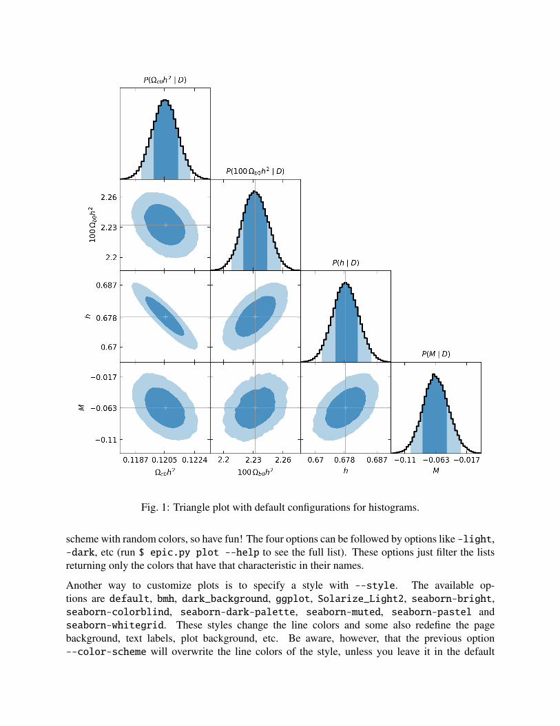
Fig. 1: Triangle plot with default configurations for histograms.

scheme with random colors, so have fun! The four options can be followed by options like -light,-dark, etc (run $ epic.py plot --help to see the full list). These options just filter the listsreturning only the colors that have that characteristic in their names.

Another way to customize plots is to specify a style with --style. The available op-tions are default, bmh, dark_background, ggplot, Solarize_Light2, seaborn-bright,seaborn-colorblind, seaborn-dark-palette, seaborn-muted, seaborn-pastel andseaborn-whitegrid. These styles change the line colors and some also redefine the pagebackground, text labels, plot background, etc. Be aware, however, that the previous option--color-scheme will overwrite the line colors of the style, unless you leave it in the default

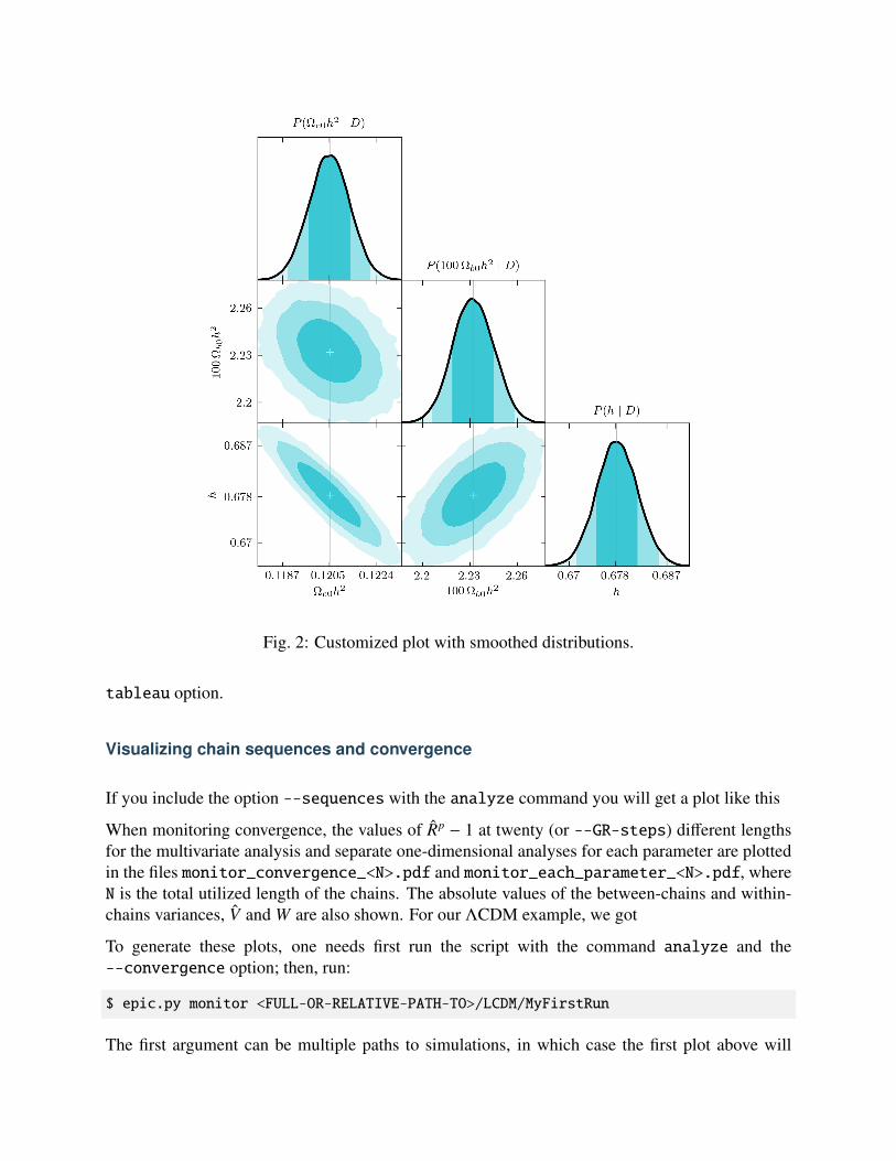
Fig. 2: Customized plot with smoothed distributions.

tableau option.

Visualizing chain sequences and convergence

If you include the option --sequences with the analyze command you will get a plot like this

When monitoring convergence, the values of Rp − 1 at twenty (or --GR-steps) different lengthsfor the multivariate analysis and separate one-dimensional analyses for each parameter are plottedin the files monitor_convergence_<N>.pdf and monitor_each_parameter_<N>.pdf, whereN is the total utilized length of the chains. The absolute values of the between-chains and within-chains variances, V and W are also shown. For our ΛCDM example, we got

To generate these plots, one needs first run the script with the command analyze and the--convergence option; then, run:

$ epic.py monitor <FULL-OR-RELATIVE-PATH-TO>/LCDM/MyFirstRun

The first argument can be multiple paths to simulations, in which case the first plot above will

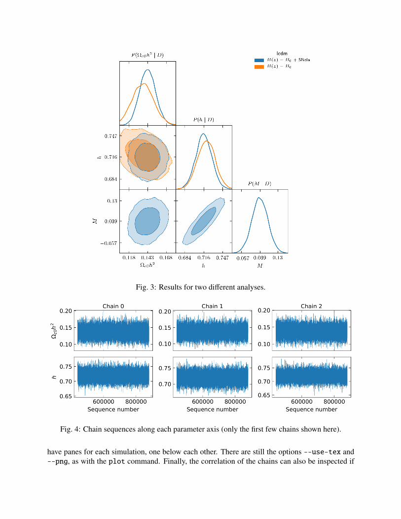
Fig. 3: Results for two different analyses.

Fig. 4: Chain sequences along each parameter axis (only the first few chains shown here).

have panes for each simulation, one below each other. There are still the options --use-tex and--png, as with the plot command. Finally, the correlation of the chains can also be inspected if

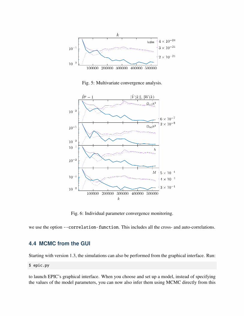
Fig. 5: Multivariate convergence analysis.

Fig. 6: Individual parameter convergence monitoring.

we use the option --correlation-function. This includes all the cross- and auto-correlations.

4.4 MCMC from the GUI

Starting with version 1.3, the simulations can also be performed from the graphical interface. Run:

$ epic.py

to launch EPIC’s graphical interface. When you choose and set up a model, instead of specifyingthe values of the model parameters, you can now also infer them using MCMC directly from this

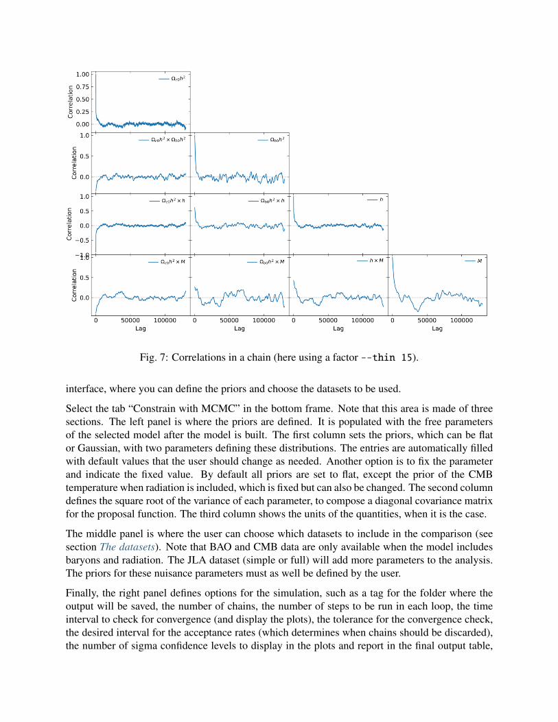
Fig. 7: Correlations in a chain (here using a factor --thin 15).

interface, where you can define the priors and choose the datasets to be used.

Select the tab “Constrain with MCMC” in the bottom frame. Note that this area is made of threesections. The left panel is where the priors are defined. It is populated with the free parametersof the selected model after the model is built. The first column sets the priors, which can be flator Gaussian, with two parameters defining these distributions. The entries are automatically filledwith default values that the user should change as needed. Another option is to fix the parameterand indicate the fixed value. By default all priors are set to flat, except the prior of the CMBtemperature when radiation is included, which is fixed but can also be changed. The second columndefines the square root of the variance of each parameter, to compose a diagonal covariance matrixfor the proposal function. The third column shows the units of the quantities, when it is the case.

The middle panel is where the user can choose which datasets to include in the comparison (seesection The datasets). Note that BAO and CMB data are only available when the model includesbaryons and radiation. The JLA dataset (simple or full) will add more parameters to the analysis.The priors for these nuisance parameters must as well be defined by the user.

Finally, the right panel defines options for the simulation, such as a tag for the folder where theoutput will be saved, the number of chains, the number of steps to be run in each loop, the timeinterval to check for convergence (and display the plots), the tolerance for the convergence check,the desired interval for the acceptance rates (which determines when chains should be discarded),the number of sigma confidence levels to display in the plots and report in the final output table,

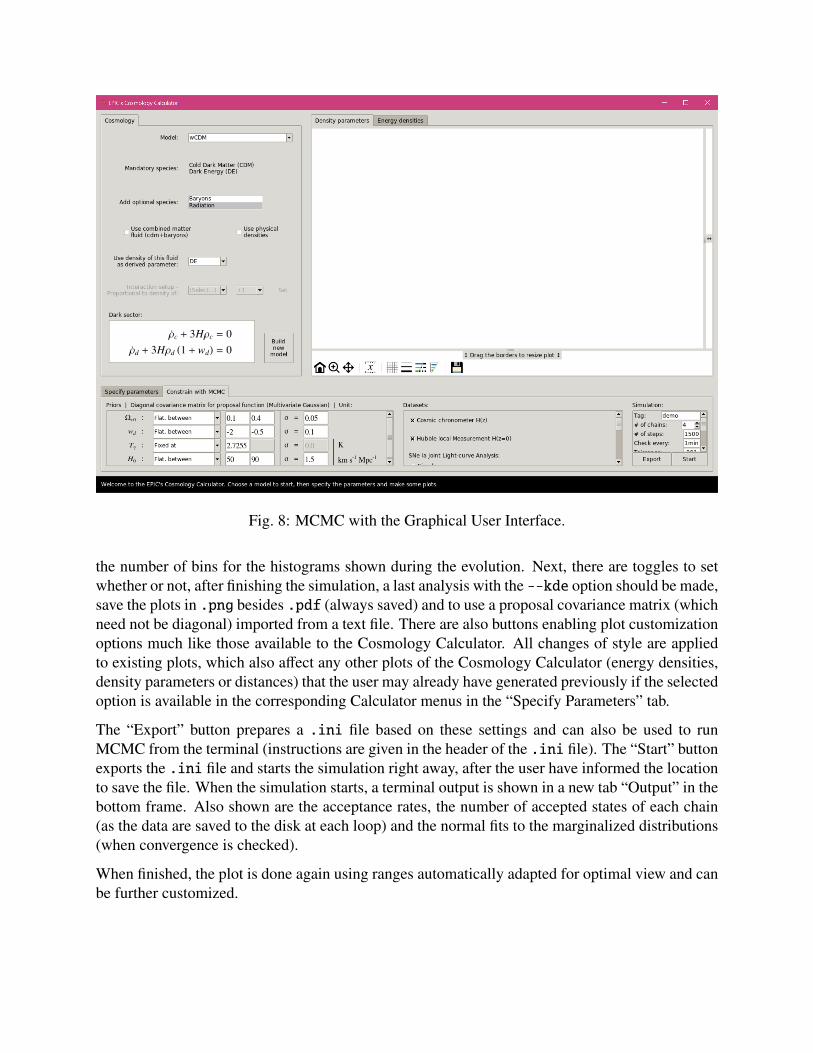
Fig. 8: MCMC with the Graphical User Interface.

the number of bins for the histograms shown during the evolution. Next, there are toggles to setwhether or not, after finishing the simulation, a last analysis with the --kde option should be made,save the plots in .png besides .pdf (always saved) and to use a proposal covariance matrix (whichneed not be diagonal) imported from a text file. There are also buttons enabling plot customizationoptions much like those available to the Cosmology Calculator. All changes of style are appliedto existing plots, which also affect any other plots of the Cosmology Calculator (energy densities,density parameters or distances) that the user may already have generated previously if the selectedoption is available in the corresponding Calculator menus in the “Specify Parameters” tab.

The “Export” button prepares a .ini file based on these settings and can also be used to runMCMC from the terminal (instructions are given in the header of the .ini file). The “Start” buttonexports the .ini file and starts the simulation right away, after the user have informed the locationto save the file. When the simulation starts, a terminal output is shown in a new tab “Output” in thebottom frame. Also shown are the acceptance rates, the number of accepted states of each chain(as the data are saved to the disk at each loop) and the normal fits to the marginalized distributions(when convergence is checked).

When finished, the plot is done again using ranges automatically adapted for optimal view and canbe further customized.

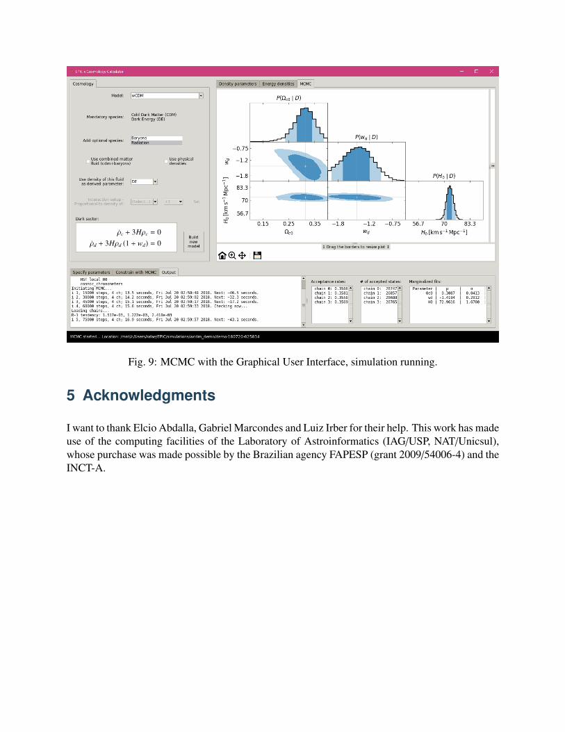
Fig. 9: MCMC with the Graphical User Interface, simulation running.

5 Acknowledgments

I want to thank Elcio Abdalla, Gabriel Marcondes and Luiz Irber for their help. This work has madeuse of the computing facilities of the Laboratory of Astroinformatics (IAG/USP, NAT/Unicsul),whose purchase was made possible by the Brazilian agency FAPESP (grant 2009/54006-4) and theINCT-A.

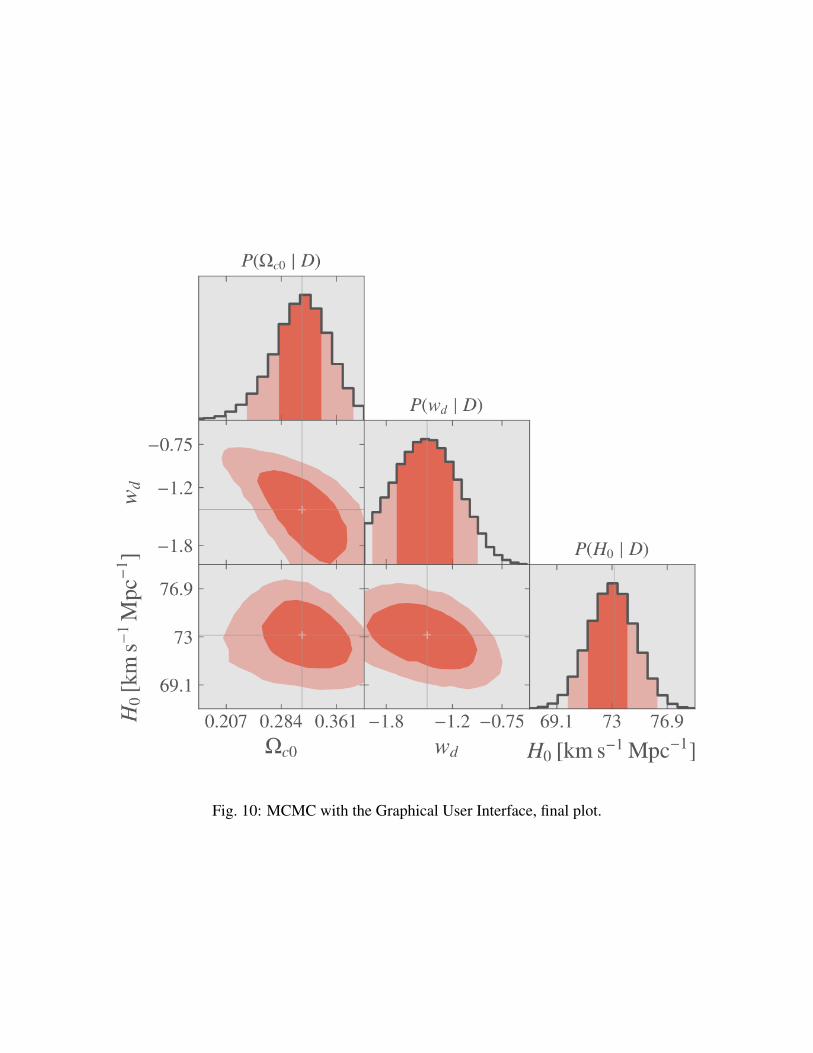
Fig. 10: MCMC with the Graphical User Interface, final plot.