A Multi-domain spectral method for supersonicreactive ows

Wai-Sun Don, David Gottlieb & Jae-Hun Jung 1

Brown University, Division of Applied Mathematics, 182 George Street,Providence, RI 02912

E-mail: wsdon, dig, jung@cfm.brown.edu

Version: April 10, 2002

This paper has a dual purpose: it presents a multidomain Chebyshev method forthe solution of the two-dimensional reactive compressible Navier-Stokes equations,and it reports the results of the application of this code to the numerical simulationsof high Mach number reactive ows in recessed cavity. The computational methodutilizes a newly derived interface boundary conditions as well as an adaptive �lteringtechnique to stabilize the computations. The results of the simulations are relevantto recessed cavity ameholders.

Key Words: Multi-domain spectral method, Penalty interface conditions,Supersonic combustor, Recessed cavity ame-holder, Compressible Navier-Stokesequations

1. INTRODUCTION

The eÆcacy of spectral methods for the numerical solution of highly supersonic,reactive ows had been previously reported in the literature. Don and Gottlieb[7, 8] simulated interactions of shock waves with hydrogen jets and obtained resultsshowing the rich dynamics of the mixing process as well as the very complex shockstructures. Don and Quillen [9] studied the interaction of a planar shock with acylindrical volume of a light gas and showed that the spectral methods used gavegood results for the ows with the shocks and complicated non-linear behaviors. Infact the results compared favorably to ENO schemes.

The methods reported above were based on Chebyshev techniques in one do-main. In order to extend the utility of spectral methods to complex domains,multidomain techniques have to be considered. The main issue here is the sta-ble imposition of the interface boundary conditions, and in this paper we considermainly the penalty method, introduced for hyperbolic equations by Funaro andGottlieb [10, 11].

There is an extensive literature on the subject: Hesthaven [13, 14, 15] appliedpenalty BC for Chebyshev multidomain methods using the characteristic variables.Carpenter et. al. [4, 18, 19] used it in conjunction with compact �nite di�erenceschemes, going from a scalar model equation to the full N-S equations in generalcoordinate systems. Carpenter, Gottlieb and Shu [5] demonstrated the conservationproperties of the Legendre multidomain techniques.

In the current work we follow the same methodology but in the context of su-personic combustion. We formulate the stable interface conditions based on the

1This work was performed under AFOSR grant no. F49620-02-1-0113 and DOE grant no.

DE-FG02-96ER25346.

1

penalty method in a conservative form for both Euler and Navier-Stokes equationsin two dimensional Cartesian coordinates. We derive stability conditions, inde-pendent on the local ow properties, for the penalty parameters for the Legendrespectral method. We also present here a new adaptive �ltering technique thatstabilize the spectral scheme when applied to supersonic reactive ows.

Implementing this method, we consider supersonic combustion problems in re-cessed cavities in order to establish the eÆcacy of recessed cavity ame-holders.

We consider two di�erent cases; (1)Non-reactive ows with two chemical speciesand (2)Reactive ows with four chemical species.

Recessed cavities provide a high temperature, low speed recirculating region thatcan support the production of radicals created during chemical reactions. This sta-ble and eÆcient ame-holding performance by the cavity is achieved by generatinga recirculation region inside the cavity where a hot pool of radicals forms resultingin reducing the induction time and thus obtaining the auto-ignition [2, 23]. Ex-periments have shown that such eÆciency depends on the geometry of the cavitysuch as the degree of the slantness of the aft wall and the length to depth ratioof cavity L=D. Thus one can optimize the ame-holding performance by properlyadjusting the geometrical parameters of the cavity ame-holder system for a givensupersonic ight regime. There are two major issues of such cavity ame-holdersystem that need to be investigated ; (1)What is the optimal angle of the aft wallfor a given L=D? and (2)How does the fuel injection interact with cavity ows? Ananswer to these questions require both a comprehensive laboratory and numericalexperiments.

There have been previous numerical studies on these questions, many of themrely on the turbulence models. Rizzetta [20] used a modi�cation of the BaldwinLomax algebraic turbulence model. Davis and Bowersox [6] also used Baldwin-Lomax model. Zhang et.al. [24] used Wilcox �� ! turbulence model. Baurle andGruber [3] used the Menter model. Although the use of the turbulence models canmake it possible to handle the compressible supersonic shear ows, the results arequite model-dependent as they require parametric assumptions. In this work, wesolve the full compressible Navier-Stokes equations with chemical reactions withoutany turbulence model, using a multi-domain spectral method.

Results of several numerical studies including the present study have shown thatthe stability of the recirculation inside cavity is enhanced for the lower angle ofcavity compared to the rectangular cavity. The present study, however, gives moreaccurate and �ner details of the �elds than those done by lower order numericalexperiments. We show that a stationary recirculation region is not formed inside thecavity contrary to what the lower order schemes predict. A quantitative analysismade in this study shows that the lower angled wall of the cavity reduces thepressure uctuations signi�cantly inside the cavity for the non-reactive ows. Weobtained a similar result for the reactive ows with the ignition of the fuel suppliedinitially in the cavity.

The rest of this paper is organized as follows. In section 2 the governing equa-tions are given. In section 3 we describe the numerical method used in this work.In this section we present the adaptive-�ltering used to remove the high frequencymode that causes the instability due to the non-smoothness of the ow, and wederive stable penalty interface conditions. In section 4 the system of the supersonicrecessed cavity combustor is described. In section 5 the main results of this workare given and discussed.

2

2. THE GOVERNING EQUATIONS

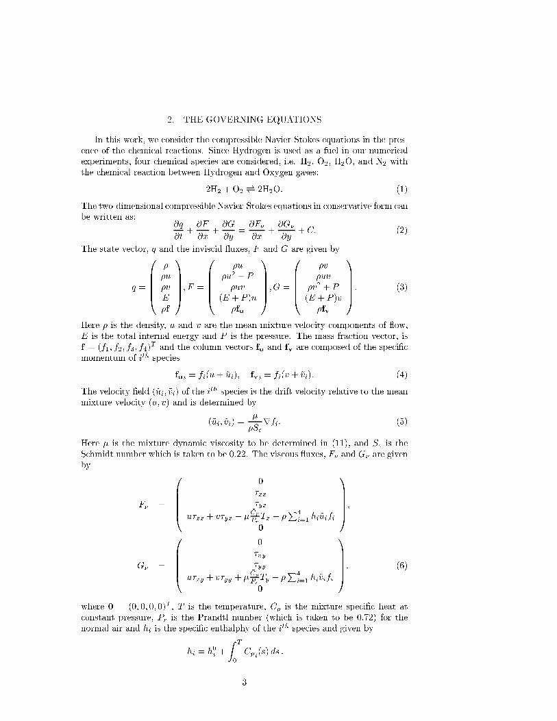
In this work, we consider the compressible Navier-Stokes equations in the pres-ence of the chemical reactions. Since Hydrogen is used as a fuel in our numericalexperiments, four chemical species are considered, i.e. H2, O2, H2O, and N2 withthe chemical reaction between Hydrogen and Oxygen gases:

2H2 +O2 *) 2H2O: (1)

The two-dimensional compressible Navier-Stokes equations in conservative form canbe written as:

@q

@t+@F

@x+@G

@y=@F�@x

+@G�

@y+ C: (2)

The state vector, q and the inviscid uxes, F and G are given by

q =

0BBBB@

��u�vE�f

1CCCCA; F =

0BBBB@

�u�u2 + P�uv

(E + P )u�fu

1CCCCA; G =

0BBBB@

�v�uv

�v2 + P(E + P )v

�fv

1CCCCA: (3)

Here � is the density, u and v are the mean mixture velocity components of ow,E is the total internal energy and P is the pressure. The mass fraction vector, isf = (f1; f2; f3; f4)

T and the column vectors fu and fv are composed of the speci�cmomentum of ith species

fui = fi(u+ ~ui); fvi = fi(v + ~vi): (4)

The velocity �eld (~ui; ~vi) of the ith species is the drift velocity relative to the mean

mixture velocity (u; v) and is determined by

(~ui; ~vi) =�

�Scrfi: (5)

Here � is the mixture dynamic viscosity to be determined in (11), and Sc is theSchmidt number which is taken to be 0:22. The viscous uxes, F� and G� are givenby

F� =

0BBBB@

0�xx�yx

u�xx + v�yx + ��Cp

PrTx � �

P4i=1 hi~uifi

0

1CCCCA;

G� =

0BBBB@

0�xy�yy

u�xy + v�yy + ��Cp

PrTy � �

P4i=1 hi~vifi

0

1CCCCA: (6)

where 0 = (0; 0; 0; 0)T , T is the temperature, �Cp is the mixture speci�c heat atconstant pressure, Pr is the Prandtl number (which is taken to be 0:72) for thenormal air and hi is the speci�c enthalphy of the ith species and given by

hi = h0i +

Z T

0

Cpi(s) ds :

3

where h0i is the reference enthalpy of the ith species and the speci�c heat of the ith

species at constant pressure, Cpi is represented as a fourth-order polynomial of T(see [17]). The elements of the viscous stress tensor are given by

�xixj = �

�@ui@xj

+@uj@xi

�+ Æij�

2Xk=1

@uk@xk

; (7)

where Æ is the kronecker delta symbol, and � is the bulk viscosity which is taken tobe � 2

3� under the Stokes hypothesis.The equation of state is given by the assumption of the perfect gas law

P = � �RT = RT

4Xi=1

�fi=Mi; (8)

where �R is a mixture gas constant with the universal gas constant R and Mi is themolecular weights of ith species. The energy E is given by

E = �

Z T

0

�Cp(s)ds� P +1

2�(u2 + v2) +

4Xi=1

�fih0i ; (9)

where the mixture speci�c heat at constant pressure is given by

�Cp =

4Xi=1

Cpifi=Mi: (10)

2.1. The chemical models

We use the same models as in [7]. Each chemical species has di�erent dynamicalviscosity �i based on Sutherland's law and we obtain the mixture viscosity � byWilke's law [22], i.e.

�i�0i

=

�T

T0i

�3=2�T0i + SiT + Si

�;

� =

4Xi=1

�ifi=MiP4j=1 fj=Mj�ij

; (11)

�ij =

�1 + [(�i=�j)(fj=fi)]

1

2 (Mi=Mj)1

4

�2[8(1 + (Mi=Mj))]

1

2

:

Here �0i, T0i and Si are constants. A modi�ed Arrhenius Law gives the equilibriumreaction rate ke, the forward reaction rate kf and the backward reaction rate kb as

ke = AeT exp(4:60517(Ee=T � 2:915))

kf = Af exp(�Ef=(RT ))

kb = kf=ke;

where the activation energy Ee = 12925; Ef = 7200 and the frequency factor Ae =83:006156; Af = 5:541� 1014.

A table of the constants is given in Appenix C.

4

The species are ordered as follows : (H2, O2, H2O, N2), and the law of massaction is used to �nd the net rate of change in concentration of ith species _Ci bythe single reaction (1), i.e.

_C1 = 2(kf [H2]2[O2]� kb[H2O]

2)

_C2 = �(kf [H2]2[O2]� kb[H2O]

2)

_C3 = 2(kf [H2]2[O2]� kb[H2O]

2)

where [�] denoted the net rate of change in concentration.Finally, the chemical source term C in (2) is given by

C =�0; 0; 0; 0; _C1M1; _C2M2; _C3M3; _C4M4

�T; (12)

where _Ci is the net rate of change in concentration of ith species by the reaction.In Appendix C, all the necessary coeÆcients and constants used for the reactive

Navier-Stokes equations with species (H2, O2, H2O, N2) are given.

3. THE MULTI-DOMAIN SPECTRAL METHOD

In this section we describe the two crucial components of the Chebyshev multidomain code used in our work, i.e. the adaptive �ltering and the penalty methodfor the stable interface conditions.

3.1. The Adaptive Filtering Technique

It is well known that spectral methods may exhibit instabilities when appliedto nonlinear equations. To stabilize the spectral scheme in an eÆcient way we usehere �lters to attenuate the high frequency modes of the function qN(x; t) smoothlyto zero. Thus the �ltered version of a polynomial qN is given by:

q�N(x; t) =

NXk=�N

�(k=N)ak(t)�k(x); (13)

where ak is the transform coeÆcient and �k is the basis polynomial of order k(generally the Fourier and Chebyshev polynomials for a periodic and non-periodicfunction respectively.)

Following Vandeven [21] we de�ne a �lter function �(!) of order p > 1 as aC1[�1; 1] function satisfying

�(0) = 1 ; �(�1) = 0 ;�(j)(0) = 0 ; �(j)(�1) = 0 ; j � p

(14)

where �(j) denotes the j-th derivative.It can be shown that the �ltered sum (13) approximates the original function

very well away from the discontinuities. A good example of �lter function is theexponential �lter. It is de�ned as

�(!) = exp (��j!j ) ; (15)

where �1 � ! = k=N � 1, � = � ln �, � is the machine zero and is the order ofthe �lter.

5

The exponential �lter o�ers the exibility of changing the order of the �ltersimply by specifying a di�erent . One does not have to write a di�erent �lter fordi�erent order. Thus varying with N yields exponential accuracy according to[21]. In the present study the sixth order global smoothing ( = 6) is used. If theorder of the �lter is taken to be too small, say � 4, the method becomes toodissipative

In the current application, the interaction of the aft cavity wall and the strongvortex generated by the shear layer ow over the cavity, creates large pressurevariations near the corner of the aft cavity wall. The local sharp gradient can causenumerical instability and a heavier �lter is needed to prevent the development ofoscillations in this region. This heavy �ltering can be used globally and maintainthe stability of the scheme, however this dissipates out all �ne scale structures,which is highly undesirable when the resolution of �ne scale structures is essentialfor the understanding of the recessed cavity ameholder systems.

Since this is a local phenomenon, it is enough to apply a heavy �lter only inpoints in this region. This Local Adaptive Filtering keeps the scheme stable, withoutdissipating �ne scale features away from this region. The local adaptive �ltering iscarried out where conditions such as ql � q � qu are violated. Here q can be themass fraction of each species fi and/or temperature T and ql and qu denote thelower and upper tolerance limits of q. In this work, a �ltering of the order = 2or = 3 is used to reduce the magnitude of the oscillations at those points.

The results of this work indicate that the local adaptive �ltering is applied onlyin a few number (in the range of 1 to 7) of grid points around the corner of the aftwall once in a while.

3.2. Stable Interface Conditions

In this paper we use mainly the penalty type interface conditions, i.e. theboundary conditions are imposed only in a weak form [10, 11]. Successful penaltyinterface conditions were constructed based on the characteristics for the Navier-Stokes equations in [13, 14, 15] and for spectral method and for high-order �nitedi�erence methods in [4, 18, 19], and a conservative form of penalty interface con-ditions was proposed [5] for the Legendre spectral method. Following the same ideaas those works, we consider two interface conditions, i.e.

1. The averaging method, in which the interface conditions are obtained by av-eraging the state vectors of the two adjacent domains, and

2. The Penalty method in conservative form in which the interface conditionsare satis�ed only in a weak form, leaving the approximations not necessarilycontinuous at the interfaces.

In the following sections we will give the penalty interface conditions for theEuler and Navier-Stokes equations and also show that the averaging method is asubset of the penalty method.

3.2.1. Conservative Penalty Interface Conditions

Consider Eq.(2) with the inviscid part only, in the x-direction in the interval�1 � x � 1, i.e.,

@q

@t+@F

@x= 0: (16)

6

For simplicity, assume that we have two domains in this interval with the interfaceat x = 0, qIN (x; t) denotes the numerical solution in the left domain x � 0 andqIIM (x; t) in the right domain x � 0. Note that the numerical solution is composedof two polynomials of di�erent orders. The Legendre spectral penalty method isgiven by

@qIN@t

+@IINF (q

IN )

@x= B(qIN (�1; t)) +

�1QN(x)[f+(qIN (0; t))� f+(qIIM (0; t))] +

�2QN(x)[f�(qIN (0; t))� f�(qIIM (0; t))];

@qIIM@t

+@IIIM F (qIIM )

@x= B(qIIM (1; t)) +

�3QM (x)[f+(qIIM (0; t))� f+(qIN (0; t))] +

�4QM (x)[f�(qIIM (0; t))� f�(qIN (0; t))] (17)

where B is a boundary operator at the end points, i.e., x = �1 and IIN and IIIM arethe Legendre interpolation operators for the left and right domains respectively. .The positive and negative uxes f+ and f� are de�ned by

f� =

ZS��S�1dq; (18)

with

A �@F

@q= S�S�1: (19)

The Jacobian matrix A is assumed to be symmetric. �+ and �� are the diagonalmatrices composed of positive and negative eigenvalues of A respectively. QN (x)and QM (x) are polynomials of orders N andM respectively such that they are zeroat all the collocation points except the interface points x = 0 (for example QN(x) =(1�x)T 0

N (x)N2 ; 0 � x � 1 where TN (x) is the Chebyshev polynomial of degree N). The

penalty parameters �1; �2; �3 and �4 are all constants. Since we are interested only inthe interface conditions, we ignore the boundary operator B at x = �1. De�ne thediscrete scalar product (p; q)N =

PNi=0 p

T (�i)q(�i)!i. !i is the weight in the Gauss-Lobatto-Legendre quadrature formula. With the discrete product, the energy E(t)is de�ned by E(t) = (qIN (x; t); q

IN (x; t))N + (qIIM (x; t); qIIM (x; t))M . The stability

conditions of penalty parameters are given by the following theorem [5]:

Theorem 1. The energy is bounded by the initial energy of the system if thefollowing conditions are satis�ed ;

2!IN�1 � 1; 2!IN�2 � 1; 2!IIM �3 � �1; 2!IIM �4 � �1;

!IN�1 � !IIM �3 = 1; !IN�2 � !IIM �4 = 1: (20)

3.2.2. The Penalty Method for the Euler Equations

The penalty method in the case of the 2-D Euler equation is given by

@qN@t

+@INF (qN )

@x+@ING(qN )

@y= �1;3Q(x; y)[f

+(qN )� f+(qM�)] +

�2;4Q(x; y)[f�(qN )� f�(qM�)]; (21)

7

where qM� is the state vector of the adjacent domain at the interface of degreeM, �1;3(�2;4) denotes �1(�2) and �3(�4) respectively. �1 and �2 (�3 and �4) are thepenalty parameters for the right(left) in x-direction and top(bottom) in y-directionrespectively. Q(x; y) is a polynomial which vanishes at all of interior points of thedomain and is equal to 1 at the four interfaces. Note that the boundary operatorB does not appear in the scheme. Let A be the linearized Jacobian matrix (arounda state vector q0) of two inviscid uxes

A =

�@F

@q;@G

@q

�� ~njq0 : (22)

where ~n = (nx; ny) is the unit outward normal vector. Since the matrix A issymmetric, there exists S such that

A = S�S�1; (23)

where � is a diagonal matrix composed of eigenvalues of A. Then A = A+ + A�

and A� = S��S�1. �� is de�ned as in previous section. Splitting A yields

f� = A�q0; : (24)

where f� is obtained from the linearized state.

Remark 1. Since ~n = (nx; ny) is taken to be outward normal vector, the stabilitycondition (20) is now given by

2!IN�1 � 1; 2!IN�2 � 1; 2!IIM �3 � 1; 2!IIM �4 � 1;

!IN�1 + !IIM �4 = 1; !IN�2 + !IIM �3 = 1: (25)

The Jacobian matrix A and its eigenvalue matrix � are given in Appendix A.

Example

-0.02 -0.01 0 0.01 0.02-0.02

-0.01

0

0.01

0.02

-0.02 -0.01 0 0.01 0.02-0.02

-0.01

0

0.01

0.02

FIG. 1 The propagation of a density peak with the penalty Euler equations: Theinitial condition (left) and the approximations (right) at t = 0:03604ms are given.The physical domain is partitioned with 16 rectangular sub-domains.

To demonstrate the above formulation for the Euler Equations, we considerthe propagation of a Gaussian density peak at the center of rectangular physical

8

domains. The physical domain is partitioned with 16 sub-domains. The inter-face conditions between the domains are imposed according to the penalty Eulerequations as discussed above. Characteristic boundary conditions are imposed atthe outer physical boundaries. The results presented in �gure 1 indicate that thepenalty formulation works well. From the numerical experiments of this problem,we observe that re ections can be created at the interface across the adjacent do-mains depending on the choice of the penalty parameters. Thus proper choice ofthe penalty parameters should take into account re ections from the interfaces. Wewill return to this issue in a future paper [16].

3.2.3. The Penalty Method for the Navier-Stokes Equations

When dealing with the Navier Stokes equation, we keep the penalty form forthe Euler uxes and add a penalty term for the viscous uxes. The stability ofthis procedure stems from the fact that the Jacobian matrices for the full reactiveNavier-Stokes equation can be symmetrized by the same similarity transformation(see Appendix B). Thus we get the system:

@qN@t

+@INF

@x+@ING

@y=

@INF�@x

+@ING�

@y+

�1;3Q(x; y)[f+(qN )� f+(qM�)] +

�2;4Q(x; y)[f�(qN )� f�(qM�)] +

�6;8Q(x; y)[A� � qN �A� � qM�] +

�5;7Q(x; y)[A� � @qN �A� � @qM�]: (26)

Here f� are same as de�ned in the previous section and the Jacobian matrix vectorA� is given by

A� =

�@F�@qx

nx;@G�

@qyny

�jq0 ; (27)

andq = (q; q); @q = (qx; qy); (28)

where again q� and @q� denote the adjacent domains state vectors and theirderivatives. Note that the penalty terms A� � @q does not appear in [4, 18, 19].The penalty parameters �5;7 and �6;8 are de�ned in the same way as in the previoussection. To seek stable penalty parameters we split the inviscid and viscous uxesand keep the stability conditions of �1;2;3;4 for the inviscid ux as in Theorem 1.The stability conditions of �5;7 and �6;8 are given in the following Theorem :

Theorem 2. The penalty method for the Navier-Stokes equations (26) is stableif the penalty parameters �j , j = 1:::4 are as in Theorem 1 and the rest satisfy:

!N�6 � 0;

!N�6 � !M�8 = 0;

1 + !N�5 � !M�7 = 0;�1

!M+

1

!N

�!2M�

27 � 2�7 + 4!N�6 +

1

!M� 0 (29)

in addition to the conditions speci�ed for �1; �2; �3 and �4 in Theorem 1.

Proof.

9

As in the proof of Theorem 1, we assume that we have two domains and bymultiplying the equations by the state vectors, we get

1

2

d

dtE(t) � [Inviscid] + [V iscous]; (30)

where [Inviscid] and [V iscous] denote the terms from inviscid and viscous parts ofthe equation respectively. The conditions for �1;2 and �3;4 given in the Theorem 1assure that the �rst term [Inviscid] is negative. The [V iscous] part at the interfaceis given by

[V iscous] = qTA�q0 �

NXi=0

q0iTA�q

0

i!i �

qT�A�q0

� �MXj=0

q0i�TA�q

0

i�!j +

�5!N [qTA�q

0 � qTA�q0

�] + �7!M [qT�A�q0

� � qT�A�q0] + (31)

�6!N [qTA�q � qTA�q�] + �8!M [qT�A�q� � qT�A�q];

where q0 denotes the derivative of q either in x or y direction, ! is the Legendreweight, and A� is

A� =

�@F�@qx

;@G�

@qy

�� ~njq0 : (32)

Since all the eigenvalues of A� are non-negative, every term inside the summationsin the above equation is not negative, and we would like to keep the boundaryterms. Thus we get the energy estimate such as

1

2

d

dtE(t) � [qTA�q

0 � !Nq0TA�q

0 � qT�A�q0

� � !Mq0T� A�q

0

�] +

�5!N [qTA�q

0 � qTA�q0

�] + �7!M [qT�A�q0

� � qT�A�q0] +

�6!N [qTA�q � qTA�q�] + �8!M [qT�A�q� � qT�A�q] : (33)

The RHS of (33) can be rewritten as

RHS = uTBu; (34)

where u = (q; q�; q0; q0�) and B is given by

B =

0BB@

2�6A� ��6A� � �8AT� (1 + �5)A� ��5A�

��6AT� � �8A� 2�8A� ��7A� (�1 + �7)A�

(1 + �5)AT� ��7A

T� �2!NA� 0

��5AT� (�1 + �7)A

T� 0 �2!MA�

1CCA (35)

with 0 = diag(0; 0; 0; 0); �5 = !N�5; �6 = !N�6; �7 = !M�7 and �8 = !M �8: It issuÆcient for the proof if B can be shown to be negative semi-de�nite. This �rstleads to:

!N�6 � 0; !N�6 = !M �8; 1 + !N�5 � !M�7 = 0: (36)

Note that we use here the fact that A� is symmetrizable (see Appendix B). Takinginto account (36), B becomes

B =

0@ 2�6 ��7 �1 + �7

��7 �2!N 0�1 + �7 0 �2!M

1A : (37)

10

To ensure negative semi-de�niteness, det(B) � 0 and therefore�1

!M+

1

!N

��27 � 2

1

!M�7 + 4�6 +

1

!M� 0: (38)

Thus��7 � �7 � �+7 (39)

where

��7 =1

!M + !N�

s�!M!N(1 + 4�6(!M + !N ))

(!N + !M )2:

Here we note that the condition that �6 ��1

4(!N+!N ) must be satis�ed in order for

�7 to have real roots. This yields the conditions in the Theorem.

Note that these conditions are given independently of the local ow proper-ties. And moreover, the penalty parameters of each domain are constrained by itsadjacent domain.

Remark 2. For ~n to be outward normal vector the condition (40) is now givenby

!N�6 � 0; !N�6 + !M�8 = 0; 1 + !N�5 + !M �7 = 0;�1

!M+

1

!N

�!2M�

27 + 2�7 + 4!N�6 +

1

!M� 0 (40)

with the conditions (25)

3.2.4. The Averaging Method

We show in this Section that the averaging method can also be written as apenalty method with a particular choice of the parameters.

Euler Equations : We start �rst with the Euler equations: consider the follow-ing penalty method:

@q

@t+@F

@x+@G

@y= �1;3Q(x; y)[f

0+(q)� f 0+(q�)] +

�2;4Q(x; y)[f0�(q)� f 0

�(q�)]; (41)

wheref 0� =

�A�qx; A

�qy�� ~njq0 ; (42)

Note that the penalty terms use the derivative of the uxes.

Theorem 3. If �1 = �3 =12 , �2 = �4 =

12 then the above penalty method (41)

is equivalent to the averaging method and is stable.

Proof. We prove the theorem at the interface x = 0 with the rectangular domainand assume thatN =M . If �1 = �3 =

12 , and �2 = �4 =

12 then the method becomes

@qI

@tjx=0 =

@qII

@tjx=0 = �

1

2

�@F I

@x+@F II

@x

��@G

@y(43)

11

and this is obviously equivalent to the Averaging Method. Here note that @GI

@y =@GII

@y = @G@y . Following the same procedure in Theorem 2, the energy equation

becomes

1

2!N

d

dtE(t) = �

1

2!N

�qIAqI � qIIAqII

�j0 + (�1q

I � �3qII)A+(qIx � qIIx )j0

+(�2qI � �4q

II)A�(qIx � qIIx )j0: (44)

Since �1 = �3 =12 , �2 = �4 =

12 , and q

I(0; y; t) = qII(0; y; t), the RHS of the aboveequation vanishes and the energy is bounded by the initial energy.

The Navier-Stokes Equations : The averaging method for the N-S equationscan be presented as

@q

@t+@F

@x+@G

@y=

@F�@x

+@G�

@y+

�1;3Q(x; y)[f0+(q)� f 0

+(q�)] +

�2;4Q(x; y)[f0�(q)� f 0

�(q�)] +

�5;7Q(x; y)[A� � @2q�A� � @

2q�] +

�6;8Q(x; y)[A� � @q�A� � @q�]; (45)

where @2q is the second derivative of q in either x or y direction.

Theorem 4. If �1 = �3 =12 , �2 = �4 =

12 , �5 = �7 =

12 , and �6 = ��8 = � 1

2!N,

then the approximation is continous at the interface and the scheme (45) is stable.

Proof. If �1 = �3 =12 , �2 = �4 =

12 , �5 = �7 =

12 , and �6 = ��8 = � 1

!N, then

(45) becomes,

@qI

@tjx=0 =

@qII

@tjx=0 = �

1

2

�@F I

@x+@F II

@x

��@G

@y

+1

2

�@F I

�

@x+@F II

�

@x

�+@G�

@y

+1

!NA� � (@q

II � @qI); (46)

and this ensures the continuity of the approximation at the interface. If the approx-imation is smooth enough such that the derivative of q is continous at the interfacethen this becomes the averaging method.

Thus we get for the energy:

1

2!N

d

dtE(t) = �

1

2!N

�qIAqI � qIIAqII � 2qIA�q

Ix + 2qIIA�q

IIx

�jx=0 �Z 0

�1

qIxA�qIxdx�

Z 0

�1

qIIx A�qIIx dx+�

(�1qI � �3q

II)A+ + (�2qI � �4q

II)A��(qIx � qIIx )jx=0 + (47)�

(�5qI � �7q

II)A�(qIxx � qIIxx) + (�6q

I � �8qII)A�(q

Ix � qIIx )

�jx=0:

12

Since qI(0; y; t) = qII(0; y; t), we have

1

2!N

d

dtE(t) � qI([(�1 � �3)A

+ + (�2 � �4)A�](qIx � qIIx ) +

(�5 � �7)A�(qIxx � qIIxx)

(�6 � �8 +1

!N)A�(q

Ix � qIIx ))jx=0: (48)

Thus if �1 = �3 =12 , �2 = �4 =

12 , �5 = �7 =

12 , and �6 = ��8 = � 1

2!N, the RHS

vanishes.

3.2.5. Adaptive averaging

To ensure the stability of the scheme at some particular collocation points wherethe solution become singular and unstable, we use the averaging method adaptivelyat selective grid points. In particular, we switched from the penalty method to theaveraging when the following criteria was satis�ed:

max

�j�� ��j

j�+ ��j;jT � T�j

jT + T�j

�� Cave; (49)

orjP � P�j

jP + P�j� Cave; (50)

where Cave is a non-negative constant. Note that Cave = 0 leads to the averagingmethod, whereas a large Cave results in the penalty method. For the value of Caveused in this paper, we found out that there were very few points in which one needsto switch from the penalty to the averaging procedure. Moreover this happenedonly at very few timesteps.

4. THE CAVITY SYSTEM AND NUMERICAL CONFIGURATIONS

In this section we describe the set up of the simulations of the recessed cavity ameholders by the spectral multi-domain technique presented above. The maingoal of this experiment is to investigate how the geometry of the aft wall a�ects the ame stability.

4.1. Physical setup

In the SCRAMJet community, a cavity with the length-to-depth ratio L=D <7 � 10 is usually categorized as an 'open' cavity since the upper shear layer re-attaches at the back face [2]. In this work, we choose the L=D of the baselinecavity to be 4 and thus the open cavity system is considered. The coordinatesof the cavity are (7cm;�1cm) for the upper left and (11cm;�2cm) for the rightbottom corners of cavity. With the length of the neck of the cavity �xed to be 4cm,we consider three di�erent angles of the right corner of the oor of the cavity ( 60; 45and 30), we then compare each one with the case of the rectangular aft wall. The uid conditions are given as followings; the free stream Mach number M = 1:91,total pressure P = 2:82(atm), total temperature T = 830:6(K) and normalizedReynolds number Re = 3:9 � 107(1=m). Note that the Reynolds number is herenormalized and has a unit of 1=[length], also the Reynolds number based on the

13

cavity dimensions is O(105). The boundary layer thickness scale is Æ = 5�10�4(m),and �nally, the wall temperature is Tw = 460:7835(K). The initial con�gurationfor the baseline cavity system is shown in Figure 2.

< ------------- L = 4 cm ------------------->

M = 1.91Re = 3.95 E+07 (1/m)Pt = 2.828522 (atm)Tt = 830.6 (K)L/D = 4δ = 0.0013

−−−−−−−−−−−−−−−−−−−−−−−>−−−−−−−−−−−−−−−−−−−−−−−>

90o

D = 1 cmInjector(d=2mm)

||||Boundary Layer

FIG. 2 The initial con�guration for the baseline cavity system.

4.2. Numerical setup

We have conducted two di�erent experiments for each of the following cases :(1) non-reacting cold ow, and (2) reacting ow . We use 9 and 17 subdomains forboth cases 1 and 2. For the out ow conditions at the exit of the system and atthe upper boundary, we mainly use a semi-in�nite mapping in order to reduce thepossible re ections at the boundaries. The characteristic boundary conditions arealso applied and will be discussed in the next section and compared to the mapping.For the case of the reactive ows, the cavity was initially �lled with Hydrogen fuelwith fuel-to-total gas ratio of 0:5. The order of the polynomial of approximationin y direction in the domain beside the wall is taken large enough to resolve theboundary layer well. Finally the adaptive �ltering is turned on if the mass fraction ofHydrogen and Oxygen exceed the range of �0:09 � fH2

� 1:09;�0:02� fO2� 0:25

and the temperature exceeds the range of 300(K) � T � 3500(K). As the shearlayer and the complex features of the ows develop, the adaptivity criteria forapplying the local smoothing is satis�ed at some points. In the calculations, weuse the 3rd and 2nd order local �ltering for the non-reactive and reactive owsrespectively. It turns out that the local smoothing was applied in very few pointsat the upper corner of the cavity wall.

For the adaptive averaging, we use the criteria constant Cave such that thedi�erence of the state vectors (or pressure) between the two adjacent domains isless than 10%. In �gure 3 the Penalty Navier-Stokes equations were consideredfor the non-reactive cold ows. As evident from the contours of the density, theapproximations were well matched at the interfaces. Here the outer boundary wasapproximated by using the characteristic conditions of the inviscid uxes. Theadaptive averaging, with the given adaptivity conditions above, took place at onlya few points. The characteristic boundary conditions using the inviscid uxes yieldgood results for both the problems of the density peak propagation and the non-reactive cold ows. As in �gure 1, we observe that there exist penalty parameterssatisfying the stability conditions that may induce re ecting modes at the interfaces.

14

x

y

0.05 0.1 0.15-0.02

-0.01

0

0.01

0.02

0.03

FIG. 3 The non-reactive cold ows with the penalty Navier-Stokes equations: thedensity contours are given in this �gure at t = 0:25ms. 17 domains are used andthe boundaries of each domain are shown.

5. RESULTS AND DISCUSSION

5.1. Pressure history

Figure 4 shows the pressure history of the non-reactive cold ows for the variousangles of the aft wall at two di�erent locations inside the cavity, i.e. at the center,(x; y) = (8:5cm;�1:5cm), and at the middle of the oor (x; y) = (8:5cm;�1:9cm).

0.6

0.8

1

1.2

1.4

1.6

1.8

0.6

0.8

1

1.2

1.4

1.6

1.8

P/P

o

0.6

0.8

1

1.2

1.4

1.6

1.8

tUo/D0 100 200 300

0.6

0.8

1

1.2

1.4

1.6

1.8

0.6

0.8

1

1.2

1.4

1.6

1.8

0.6

0.8

1

1.2

1.4

1.6

1.8

tUo/D0 100 200 300

0.6

0.8

1

1.2

1.4

1.6

1.8

P/P

o

0.6

0.8

1

1.2

1.4

1.6

1.8

FIG. 4 Pressure history for non-reactive ows: the left panel represents the pressurehistory at the center of the cavity and the right panel at the middle of the oor ofthe cavity. Each panel shows the case of 90, 60, 45 and 30 degree cavity walls fromtop to bottom.

These �gures show that the pressure uctuations in cavities with lower angleof the aft are weaker than in cavities with higher angles. It is also shown that theattenuation of the pressure uctuations are obtained both at the center and themiddle of the oor of the cavity. It is interesting to observe that the patterns of thepressure uctuations for a given angle at di�erent locations are di�erent dependingon the angle. In the case of the 30 degree aft wall, the pressure uctuations arealmost the same at the two locations considered whereas the case of 45 degree showsa di�erence in the patterns of the pressure uctuations between the two locations.The pressure uctuations at the bottom grows greater than that at the center aftersome time.

Figure 5 shows the pressure history when the heavy global �lter is applied(in this case, the 4th order �lter was used). Unlike the previous case illustratedin Figure 4, where the 6th order global �lter is used, the pressure uctuations

15

0.6

0.8

1

1.2

1.4

1.6

1.8

tUo/D

P/P

o

0 100 200 300

0.6

0.8

1

1.2

1.4

1.6

1.8

tUo/D

P/P

o

0 100 200 300

1.01

1.02

1.03

1.04

1.01

1.02

1.03

1.04

FIG. 5 Pressure history of the non-reactive ows with the use of the 4th order�lter: the left panel represents the pressure history at the center of cavity and theright panel shows the left panel in a smaller scale. Each panel shows the case of90, and 30 degree cavity walls from top to bottom. Note that the scale of the rightpanel is di�erent from the left.

x

y

0.07 0.08 0.09 0.1 0.11-0.022

-0.02

-0.018

-0.016

-0.014

-0.012

-0.01

-0.008

-0.006

-0.004

x

y

0.07 0.08 0.09 0.1 0.11-0.022

-0.02

-0.018

-0.016

-0.014

-0.012

-0.01

-0.008

-0.006

-0.004

FIG. 6 Streamlines: the left �gure shows the streamlines at t = 1:685ms for theglobal �ltering order = 4 and the right at t = 2:38ms for = 6.

eventually decay out and a large recirculation zone is formed inside the cavitywithout any severe pressure uctuations. Note that the scale in the left panelshown is the same as in Figure 4 while the right panel is shown in a smaller scalefor a closer look. This �gure shows that the large recirculation zone(s) formedinside the cavity obtained by the lower order numerical scheme is induced notphysically but rather arti�cially due to the heavy numerical dissipations. This isclearly shown in Figure 6. In this �gure a large recirculation zone is observed - thiszone is formed earlier than this streamlines are captured - when the 4th order �lteris used(left �gure) and an almost steady state is already reached as the pressurehistory indicates in Figure 5. We �nd from the numerical results that the largerecirculation is very stable once it forms. This large recirculation and the steadystate solutions are not observed in the case of = 6(right). For the case of = 6instead of the large single recirculation zone, smaller scale vortex circulations areformed and they are interacting with each other, never reaching the steady statewith time. This result shows that for these sensitive problems, high order accuracyshould be used in order to minimize the e�ect of the numerical dissipation.

Figure 7 shows the case of the reactive ows for the 90 and 30 degree aft walls.Similar features of the pressure uctuations are shown as in the non-reactive ows.However the pressure uctuations are much more attenuated for both the 90 and30 degree walls than in the non-reactive cold ows. In the reactive cases Hydrogenfuel, which was initially supplied inside the cavity was consumed. As time elapses,the fuel is consumed out with the production of the water for these cases.

These results demonstrate that simulations of cold ows do not necessarily shedlight on the behavior of reactive ows.

16

0.6

0.8

1

1.2

1.4

1.6

1.8

tUo/D

P/P

o

0 100 200 300

0.6

0.8

1

1.2

1.4

1.6

1.8

tUo/D

P/P

o

0 100 200 300

0.6

0.8

1

1.2

1.4

1.6

1.8

0.6

0.8

1

1.2

1.4

1.6

1.8

FIG. 7 Pressure history for reactive ows: the left panel represents the pressurehistory at the center of cavity and the right panel at the middle of the oor of cavity.Each panel shows the case of 90 and 30 degree cavity walls from top to bottom.

x

y

0.075 0.1 0.125

-0.02

-0.01

0

x

y

0.075 0.1 0.125

-0.02

-0.01

0

FIG. 8 The water contour of the reactive ows: the left the water density contouris given in the left �gure and its streamlines in the right �gure at t = 0:135ms.

5.2. Flow �elds

Non-reactive cold ow

Figure 9 shows the density contours and streamlines for the 90, 60, 45 and 30degree walls at the instant time t = 2:4ms. As shown in the �gure, the shearlayer is becoming weaker as the degree of angle of the aft wall and the ow �eldsare becoming more regularized for the case of the lower angle. And note that thedensity compression at the corner of the aft wall is also becoming weaker for themore slanted wall cases.

Figure 11 shows the streamlines corresponing to the each case of Figure 10.Note that compared to the non-reactive cases, the shear layers are less developedfor the reavtive cases. As the �gures of the pressure uctuation history and Figure11 indicate, the shear layers are weak for both the 90 and the 30 degree walls inthe reactive cases.

Reactive ow

Figure 10 shows the water contour inside the cavity for the di�erent angles atdi�erent time. Here we de�ne the region where the ames are generated to be sameas the region where the water is produced. As the Hydrogen fuel is consumed, thewater is produced and starts to be expelled from the cavity to the main channel. The ame-holding eÆceincy is enhanced if the chemical radicals (water in this case) arestably circulating and long lasting before they are expelled from the cavity. Figure10 shows that the lower anlged aft wall (30 degree in this case) maintains morewater than the 90 degree wall at a given time. The �gure also shows that the loweranlged aft wall holds the ame (water in this case) longer than the 90 degree wall- in the last �gure in Figure 10 at t = 2:26ms, the most water is expelled andthe only the small amonout is left in the left corner while the 30 degree wall cavityholds the water still throught the cavity. These results imply that the ame-holdingeÆciency can be increased by lowering the anlge of the aft wall of the cavity.

17

FIG. 9 The density contour and the streamline of the non-reactive ows: the leftcolumn shows the density contour for 90, 60, 45 and 30 degree walls from top tobottom and the right column shows the corresponding streamlines at t = 2:43ms.The maximum contour level is 1:8 and the minimum 0:5 with the level step size 50.

APPENDIX A: THE SIMILARITY TRANSFORM MATRICES AND THEEIGENVALUES OF THE INVISCID FLUX WITH CHEMICAL SPECIES

Air model without combustion

First consider the ideal gas composed of two chemically non-reactive species(for the ideal mono-atomic gas � the diagonal matrix and S, the diagonalizer, weregiven in [15]). � is given by

� = diag(~U � ~n+ c; ~U � ~n; ~U � ~n; ~U � ~n� c; ~U � ~n; ~U � ~n);

where ~U = (u; v), ~n = (nx; ny) is an unit outward normal vector at the interfaceand c is a local sound speed.

For simplicity we assume that

�

Z T

0

�Cp(s)ds� P � �CvT;

18

This form is used only in the analysis, as mentioned in Sec. 3.1, Cpi is expressedas a 4th order polynomial in the temperature T . The nonlinear expression of Cpimakes it diÆcult to derive the Jacobian matrices of the uxes. Our simpli�cationsis a results of assuming small coeÆcients of the high order terms of the polynomial.In the actual simulations Cv is computed appropriately using the empirical law andassumed temperature independent at each linearization step. With this assumptionS is given by

S =

0BBBBBB@

1 1 0 1 0 0u+ cnx u �ny u� cnx 0 �nyv + cny v nx v � cny 0 nx

H + c~U � ~n 12~U � ~U ~U � ~k H � c~U � ~n �c2 ~U � ~k + c

f1 a12 0 f1 a12 �cR2

Rh

f2 a21 0 f2 a21 cR1

Rh

1CCCCCCA

;

where H = (E + P )=�;Ri = R=(MiCv); Rh = R1h02 � R2h

01; Rv =

P2i=1 fiRi; � =

�1=(Rv +R2v); the tangential vector

~k = (�ny; nx) and

aij = Rv

h0j(Rih0j �Rjh0i )

; aji = Rvh0i

(Rjh0i �Rih0j ); :

Note that Rv = � 1 for the mono-atomic ideal gas with , the ratio between theheat capacities Cp and Cv .

Air model with combustion

Consider now the equations the Euler equations with four reactive species. Inthis case � and S are given by

� = diag(~U � ~n+ c; ~U � ~n; ~U � ~n; ~U � ~n� c; ~U � ~n; ~U � ~n; ~U � ~n; ~U � ~n);

and

S =

0BBBBBBBBBB@

1 1 0 1 0 0 1 1u+ cnx u �ny u� cnx 0 �ny u uv + cny v nx v � cny 0 nx v v

H + c~U � ~n 12~U � ~U ~U � ~k H � c~U � ~n �c2 ~U � ~k + c 1

2~U � ~U 1

2~U � ~U

f1 a12 0 f1 a1234 R1234 a13 a14f2 a21 0 f2 a2134 R2134 0 0f3 0 0 f3 a3124 R3124 a31 0f4 0 0 f4 a4123 R4123 0 a41

1CCCCCCCCCCA;

where all the variables are same as in the two species case except that

aijkl = �ijkl(h0j � h0k + h0l )Rv=Rh;

and

Rijkl = ��ijkl(Rj �Rk +Rl)c=Rh;

with

Rh =

4Xi=1

�ijklRi(h0j � h0k + h0l ); i; j; k; l = 1; 2; 3; 4; j < k < l;

19

�ijkl is the permutation symbol and Rv =P4

i=1 fiRi. � and S are based on thetime dependent local spatial quantities at a given time. f� is calculated at theinterface points at each time.

APPENDIX B: THE SYMMETRIZABILITY OF THE COEFFICIENTMATRICES OF THE NAVIER-STOKES EQUATIONS WITH CHEMICAL

SPECIES

In [1] it had been proven that the coeÆcient matrices of the Navier-Stokesequations (expreseed in the primitive form), of the ideal gas can be simultaneouslysymmetrized. In [12, 15] the same result was demonstrated for the conservativeform of the equations. Here we show that it is also true for the Navier-Stokesequations of the combustible gas with multiple chemical species in two dimension.

Rewrite the linearized Navier-Stokes equations (2) in conservative form withoutthe chemical source term as

@q

@t+A

@q

@x+B

@q

@y= C

@2q

@x2+D

@2q

@x@y+E

@2q

@y2;

where A = @F@q ;B = @G

@q ;C = @F�@qx

;D = @F�@qy

+ @G�

@qxand E = @G�

@qy. It is suÆcient to

consider the chemically interacting two chemical species. The coeÆcient matricesare given by

A =

0BBBBBB@

0 1 0 0 0 0�� u2 (2�Rv)u �Rvv Rv 1 2�uv v u 0 0 0

u(��H) H �Rvu2 �Rvuv (1 +Rv)u u 1 u 2

�uf1 f1 0 0 u 0�uf2 f2 0 0 0 u

1CCCCCCA;

B =

0BBBBBB@

0 0 1 0 0 0�uv v u 0 0 0�� v2 �Rvu (2�Rv)v Rv 1 2v(��H) �Rvuv H �Rvv

2 (1 +Rv)v v 1 v 2�vf1 0 f1 0 v 0�vf2 0 f2 0 0 v

1CCCCCCA;

C =

0BBBBBB@

0 0 0 0 0 0�u�1 �1 0 0 0 0�v�2 0 �2 0 0 0��12 u(�1 � �3) v(�2 � �3) �3 Æ1 Æ20 0 0 0 0 00 0 0 0 0 0

1CCCCCCA

;

D = (�1 � �2)

0BBBBBB@

0 0 0 0 0 0�v 0 1 0 0 0�u 1 0 0 0 0�2uv v u 0 0 00 0 0 0 0 00 0 0 0 0 0

1CCCCCCA

;

20

E =

0BBBBBB@

0 0 0 0 0 0�u�2 �2 0 0 0 0�v�1 0 �1 0 0 0��21 u(�2 � �3) v(�1 � �3) �3 Æ1 Æ20 0 0 0 0 00 0 0 0 0 0

1CCCCCCA

;

where U2 = 12~U � ~U;H = E+P

� ; �1 = 2�+�� ; �2 = �

� ; �3 = ��Cp

�PrCv; � = P

�Rv; � =

Rv(U2��); i = �Ri�Rvh0i ; Æi = �hifi

��Sc

; ~Æi = � Æi�3; � = E

� +P2

i=1(hi�~Æi)fi; � =

� � 2U2 and �jk = �ju2 + �kv

2 + �3� :To �nd the symmetrizer for A;B;C;D and E, we �rst consider the similarity

transform matrix SP of C such that

S�1P CSP = �C ;

where �C is a diagonal matrix composed of the eigenvalues of C. The subscript Pdenotes that this matrix is adopted from the parabolic portion of the equations [1].The diagonal matrix �C of C is given by

�C =

0BBBBBB@

0 0 0 0 0 00 �1 0 0 0 00 0 �2 0 0 00 0 0 �3 0 00 0 0 0 0 00 0 0 0 0 0

1CCCCCCA:

The diagonalizer SP is composed of the eigenvectors of C, SP and its inverse S�1Pare given by

SP =

0BBBBBB@

1 0 0 0 0 0u 1 0 0 0 0v 0 1 0 0 0

� u v 1 ~Æ1 ~Æ20 0 0 0 1 00 0 0 0 0 1

1CCCCCCA

;

S�1P =

0BBBBBB@

1 0 0 0 0 0�u 1 0 0 0 0�v 0 1 0 0 0

�� �u �v 1 �~Æ1 �~Æ20 0 0 0 1 00 0 0 0 0 1

1CCCCCCA

:

The similarity transform induced by SP , transforms the coeÆcient matricesA;B;C;D and E to

S�1P ASP =

0BBBBBB@

u 1 0 0 0 0� u 0 Rv �1 �20 0 u 0 0 00 Rv� 0 u 0 00 f1 0 0 u 00 f2 0 0 0 u

1CCCCCCA;

21

S�1P BSP =

0BBBBBB@

v 0 1 0 0 00 v 0 0 0 0� 0 v Rv �1 �20 0 Rv� v 0 00 0 f1 0 v 00 0 f2 0 0 v

1CCCCCCA;

S�1P DSP =

0BBBBBB@

0 0 0 0 0 00 0 1 0 0 00 1 0 0 0 00 0 0 0 0 00 0 0 0 0 00 0 0 0 0 0

1CCCCCCA;

S�1P ESP =

0BBBBBB@

0 0 0 0 0 00 �2 0 0 0 00 0 �1 0 0 00 0 0 �3 0 00 0 0 0 0 00 0 0 0 0 0

1CCCCCCA:

where � = Rv� � � and �i = Rv( ~Æi + h1f1) + i.Introducing a symmetrizing diagonal matrix, QTQ such as

QTQ =

0BBBBBB@

� 0 0 0 0 00 1 0 0 0 00 0 1 0 0 00 0 0 1

� 0 0

0 0 0 0 �1f1

0

0 0 0 0 0 �2f2

1CCCCCCA

we have symmetrized all the coeÆcient matrices, i.e.

QTQS�1P ASP = (QTQS�1P ASP )T ;

QTQS�1P BSP = (QTQS�1P BSP )T ;

QTQS�1P CSP = (QTQS�1P CSP )T ;

QTQS�1P DSP = (QTQS�1P DSP )T ;

QTQS�1P ESP = S�1P ESP :

APPENDIX C: CONSTANTS FOR CHEMICAL MODELS

Here we provide constants used in the chemical model for the current numericalexperiment. Table I gives the constants used to get the approximation of the speci�cheat Cpi of i

th species in the 4th order polynomial of T , i.e.

Cpi = (c1 + T (c2 + T (c3 + T (c4 + c5T ))))R=Mi;

where R is a gas constant, and Mi is a molecular weight of ith species([17]). Table

II gives the molecular weight and speci�c enthalpy for each chemical species and

22

TABLE ICoeÆcients for the approximation of the speci�c heat Cpi

O2 H2 H2O N2

c1(1=mole) 3.0809 3.4990 3.4990 3.1459c2(1=mole) 0.16962E-2 -0.18651E-3 0.14878E-2 0.99154E-3c3(1=mole) -0.76334E-6 0.46064E-6 0.87544E-7 -0.22912E-6c4(1=mole) 0.17140E-9 -0.13157E-9 -0.11499E-9 0.12181E-10c5(1=mole) -0.14116E-13 0.11679E-13 0.13495E-13 0.11024E-14

TABLE IIMolecular weights and speci�c enthalpy

O2 H2 H2O N2

M(1=mole) 32.000 2.016 18.016 28.016h0(Joule=kg) -272918.21 -4280070.46 -13973684.55 -302736.23

Table III gives the reference dynamic viscosity, temperature contants T and S inWilke's law([22]).

References

[1] S. Abarbanel and D. Gottlieb, J. Comput. Phys. 41, 1(1981).

[2] A. Ben-Yakar and R. K. Hanson, AIAA paper 98-3122 (1998).

[3] R. A. Baurle and M. R. Gruber, AIAA paper 98-0938 (1998).

[4] M. H. Carpenter, J. Nordstr�om and D. Gottlieb, ICASE NASA-CR-206921(1998).

[5] M. H. Carpenter, D. Gottlieb, C.-W. Shu, ICASE 2001-44 (2001).

[6] D. L. Davis and R. D. W. Bowersox, AIAA paper 97-3274 (1997).

[7] W. S. Don and D. Gottlieb, SIAM, J. Numer. Anal. 35, 2370(1998).

[8] W. S. Don and D. Gottlieb, AIAA 97-0538 (1997).

[9] W. S. Don and C. B. Quillen, J. Comput. Phys. 122, 244(1995).

[10] D. Funaro and D. Gottlieb, Math. Comp. 51, 599(1988).

[11] D. Funaro and D. Gottlieb, Math. Comp. 57, 585(1991).

[12] A. Harten, J. Comput. Phys. 49, 151(1983).

[13] J. S. Hesthaven and D. Gottlieb, SIAM J. Sci. Comput. 17, 579(1996).

[14] J. S. Hesthaven, SIAM J. Sci. Comput. 18, 658(1997).

[15] J. S. Hesthaven, SIAM J. Sci. Comput. 20, 62(1999).

23

TABLE IIIConstants for Wlke's law

O2 H2 H2O N2

�0(kg=m=sec) 0.1919E-4 0.08411E-4 0.1703E-4 0.1663E-4T0(K) 273.111 273.111 416.667 273.111S(K) 138.889 96.6667 861.111 106.667

[16] J. H. Jung, in preparation (2002).

[17] B. J. McBride, S. Heimel, J. G. Ehlers, and S. Gordon, NASA SP-3001 (1963).

[18] J. Nordstr�om and M. H. Carpenter, J. Comp. Physics 148, 621(1999).

[19] J. Nordstr�om and M. H. Carpenter, J. Comp. Physics 173, 149(2001).

[20] D. P. Rizetta, AIAA J 26(7), 799(1988).

[21] H. Vandeven, J. Comput. Phys. 24, 37(1992).

[22] C. R. Wilke, Chem. Phys. 18, 517(1950).

[23] X. Zhang and J. A. Edwards, Aeronaut J 94(940), 355(1990).

[24] X. Zhang, A. Rona and J. A. Edwards, Aeronaut J. (March) 129(1998).

24

t = 0:175ms

t = 0:275ms

t = 0:945ms

t = 2:26ms

FIG. 10 The water contour of the reactive ows: the water density contours aregiven in the left �gures for 90 degree wall and 30 degree wall in the right �gures.From top to bottom the instant times t are 0:175ms, 0:275ms, 0:945ms and 2:26ms.The maximum and mininum contour levels are 0.01 and 0.23 respectively with thenumber of levels 50.

25

t = 0:175ms

t = 0:275ms

t = 0:945ms

t = 2:26ms

FIG. 11 The streamlines for the reactive ows: the streamlines for 90 degree wallare shown in the left �gures and the 30 degree wall in the right. From top to bottomthe times t are 0:175ms, 0:275ms, 0:945ms and 2:51ms.

26