2 field qualification of inexpensive wireless system to...
TRANSCRIPT

1
Paper submitted to Journal of Performance of Constructed Facilities 1
Field Qualification of Inexpensive Wireless System to Monitor Micro-Meter Crack 2
Response for Structural Health Monitoring 3
C.H. Dowding PhD ASCE, PE, DPL1, M. Kotowsky MS M ASCE PE2, and T.Koegel, EI M 4
ASCE3 5
_____________________________________________ 6
Abstract: This paper describes the details of installation and operation of a commercially- 7
available wireless system to measure response of an interior cosmetic crack in a residential 8
structure over a period of a year. Wireless data loggers managed the response of low power draw 9
potentiometers that measured micrometer changes in crack width. Systems like that described 10
herein are useful to describe the performance of any component of a constructed facility that 11
involves existing cracks such as bridges, building facades, etc. Four wireless nodes were 12
deployed within and around a test home of frame construction to qualify the system for further 13
field use. Considerations for qualification included: fidelity of the measured crack response, ease 14
of installation, resolution of structural health measurement, length of operation under a variety of 15
conditions without intervention, and ease of display and interpretation of data. The article first 16
describes the components of the system and the measurement plan. It then closes with an 17
evaluation of the considerations for field qualification. 18
19
Keywords: structural health, wireless, crack, monitoring, micrometer, weather, blasting, 20
vibrations, construction 21
22
1 Professor, Dept. of Civil & Environmental Engr. Northwestern Univ. Evanston, IL 60208, [email protected] 2 Research Engineer, Infrastructure Technology Institute, Northwestern Univ. Evanston, IL 60208, [email protected] 3 Structural Engineer, Sargent and Lundy Engineers, Chicago, IL 60603, [email protected]

2
Introduction 23
This paper substantiates the ability of wireless systems to measure remotely and autonomously 24
the performance of any component of a constructed facility that involves existing cracks such as 25
bridges, building facades, etc over long periods of time. One of the first systems to move 26
wireless technology from the research lab to the field serves as the example of this class of 27
wireless systems. While there are and will be other wireless systems, this system was chosen as a 28
typical example of the wireless class for comparison with wired systems. For some time, wireless 29
systems have been on the verge of being usefully deployed in the field for structural health 30
monitoring (SHM). These systems, such as that described in this paper, have now matured to the 31
point that the data logging and communication nodes can be sustainably deployed in the field in 32
robust enclosures at an affordable price. In addition, the process of data logging, internet 33
transmission and graphical data display have also matured to the point that display of data can be 34
accomplished by the average engineer. 35
Structural health is monitored in this example by the measurement of micro-meter 36
opening and closing of cracks on the interior walls of structure. This response and the associated 37
climatological data are transmitted via a secure Internet connection in an adjacent structure back 38
to a central server where they are made available via the World Wide Web. While the nodes 39
themselves are weather proof, the displacement sensors are not. Since there are other, more 40
weather proof micro-meter displacement transducers, this interior case can also serve as an 41
example for exterior deployment. Development of inexpensive, climatologically robust 42
displacement transducers has lagged development of inexpensive data logging nodes because 43
these systems have been developed for the larger agricultural market where the emphasis is on 44
recording environmental and soil moisture conditions. The much smaller market for structural 45
health monitoring through crack displacement, the basis of this comparison, is dependent upon 46
other markets to drive accessory development. 47

3
This paper is organized about considerations for field qualification. They include fidelity 48
of the measured crack response, ease of installation, resolution of the measurements, length of 49
operation under a variety of conditions without intervention, and ease of display and 50
interpretation of data. The article first describes the components of the system and the 51
measurement plan. It then closes with an evaluation of the considerations for field qualification. 52
53
54
55
56
Instrumentation Deployment 57
Site 58
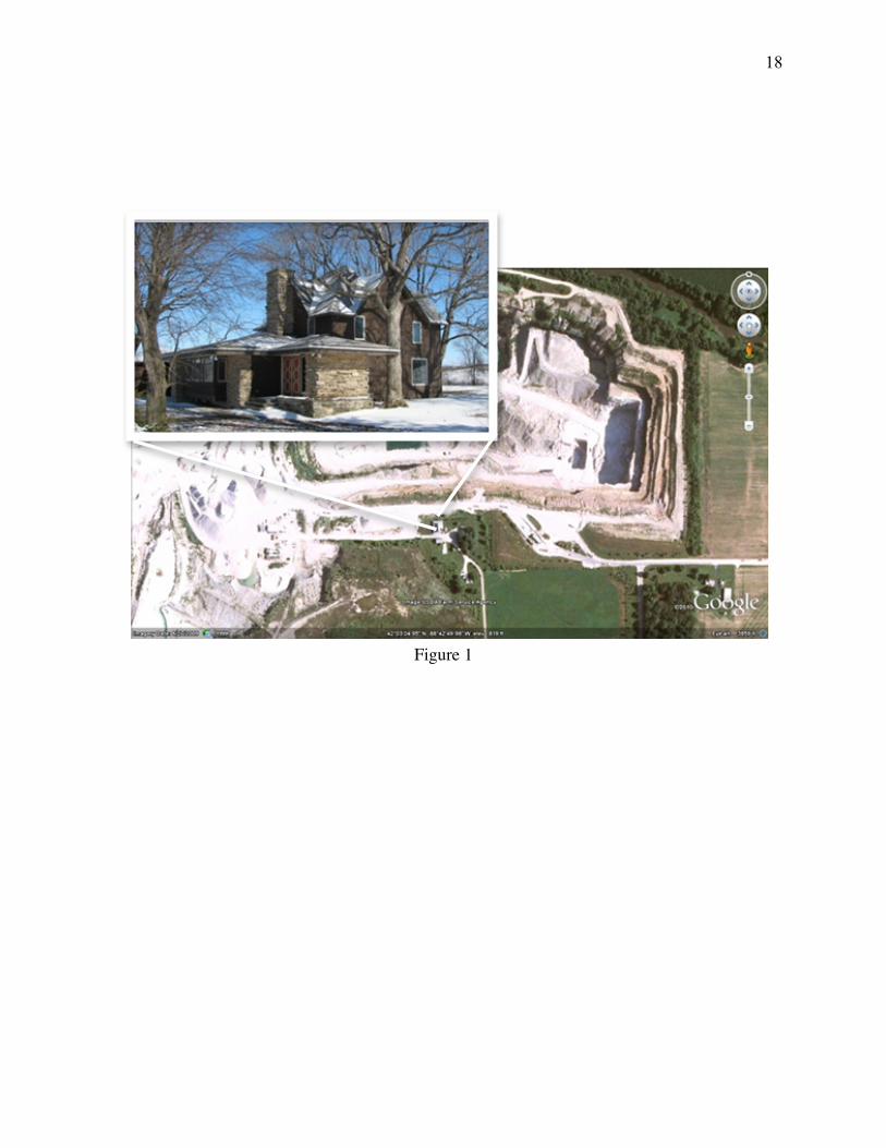
The wireless system was installed in a test house adjacent to a limestone aggregate quarry near 59
Sycamore, IL shown nestled in the trees immediately south of the quarry in Figure 1. The two-60
story house, an elevation view of which is shown in the inset to Figure 1, is typical of farm 61
homes that have seen many additions. A visit to the basement shows that there are at least two 62
additions to the house: one to the two-story frame structure and the most recent single story wrap 63
around on the west side. The house consists of a wood frame with composite wood exterior 64
siding and gypsum drywall for the interior wall covering. 65
66
Qualification plan and instrument locations 67
Four wireless nodes were deployed within and around the test structure to assess the wireless 68
system’s behavior by comparing its behavior under a variety of field conditions with that of 69
research grade wired systems (Meissner, 2010). Assessment involves fidelity of the measured 70
crack response, ease of installation, resolution of structural health measurement, length of 71
operation under a variety of conditions without intervention, and ease of operation. The 72

4
placement of nodes shown in Figure 2 was chosen to maximize the variety of operational 73
conditions. Two interior nodes (3 and 2) were chosen to compare performance of the solar cells 74
for an east and south facing window exposure as response of different cracks. Exterior nodes (4 75
and 5) were located at variable distances from the house, where the base station was deployed 76
and the base station (0) in structure that housed the Internet connection. The objective of the 77
variable distances of exterior nodes between the house and base station was to determine the 78
occurrence and necessity of multi-hopping to reach the base station. Multi-hopping describes a 79
process where nodes closer to the base station relay messages from other nodes that would not 80
otherwise be able to communicate with the base station directly. 81
82
Installation Details 83
Details and context of the nodal locations are shown in the close up photographs. External nodes 84
4 and 5, shown in Figure 3, were attached to poles and were faced to the south to maximize solar 85
exposure. Nodes 2 and 4 were employed to measure internal and external temperature and 86
humidity respectively. The manufacturer’s temperature and humidity probes can be seen attached 87
below node 4 and on the wall to the right of node 2. It was located between node 4 and the base 88
station, node 0, to provide a shorter path between node 4 and the base station. Node 4 employed 89
no external measurement devices, and was positioned to facilitate transmission from the house to 90
the base station. The need for 4 and 5 will be discussed later in the performance section. 91
Locations of the interior nodes 2 and 3 and the associated monitoring gages are shown in 92
the building plan view in Figure 4. Nodes 2 and 4 were configured to monitor interior 93
temperature and humidity as well as crack response of the large shear crack identified in the 94
photograph in Figure 5. The node itself was mounted on the window frame of the south facing 95
living room window such that its solar cells could achieve maximum solar exposure, while the 96
temperature and humidity gage module as well as the crack and null displacement gages were 97

5
mounted some 1.5meters away. Node 3 was responsible for monitoring response of the crack in 98
the second floor bedroom ceiling some 2-2.5 meters away as shown in Figure 6. It was installed 99
on the window frame of the east-facing window. 100
101
System Components 102
The example wireless system employed in this comparison with research grade wired system is 103
designed for environmental and agricultural monitoring. Each node is water and dust resistant, 104
capable of operating in wide temperature and humidity ranges, and is advertised to operate for 105
over five years with sufficient sunlight. Its weatherproof design makes it an attractive platform 106
for deployment in exterior as well as interior locations. 107
Nodes are the principal components of the Wireless Sensor Network (WSN). Its energy-108
efficient radio and sensors are designed for extended battery-life and performance, and integrates 109
IRIS family processor/radio board and antenna that are powered by rechargeable batteries and a 110
solar cell. Anode is capable of an outdoor radio range of 500ft to 1500ft depending on 111
deployment. Since the nodes form a wireless mesh network, the range of coverage can be 112
extended by simply adding additional nodes. The nodes come pre-programmed and configured 113
with a low-power networking protocol. 114
The base station, which must be connected to 110 V AC power and a network 115
connection, can transmit e-mail alerts when sensor readings cross-programmable thresholds. 116
Though the base station can be connected directly to the Internet, the test deployment described 117
herein employed a secure virtual private networking system to traverse corporate firewalls and 118
protect the system and the data. A point-to-point wireless Ethernet system was employed to 119
connect the base station to an Internet connection located in an adjacent building. 120
The base station provides multiple methods for viewing and manipulating recorded data: 121
One may use the base stations built-in web interface to perform simple plotting operations. One 122

6
may also connect to the base station using FTP or SFTP to retrieve raw data for further, more 123
sophisticated processing and Web display. The latter method was employed in the described test 124
deployment. 125
A unique feature of this system is that the node end-user need not manually program the 126
system to function properly, which is attractive to those with normal computer skills. The nodes 127
record data every thirty seconds for the first hour after activation. Thereafter they record once 128
every fifteen minutes. These data are automatically stored, retrieved once daily, processed, and 129
graphically displayed on a secure Web site. 130
During every sampling cycle, each node records its internal temperature, battery voltage, 131
and solar input voltage, along with data from up to four external sensors to which it is attached. 132
For instance, external temperature and humidity, soil moisture, and other agriculturally 133
interesting phenomenon can be recorded using sensors supplied by the manufacturer. Two nodes 134
in this demonstration were fitted with temperature and humidity probes supplied by the 135
manufacturer, as shown in the left photograph in Figure 3. 136
Nodes that were deployed to measure crack response were supplemented with a signal 137
conditioning board, available from the manufacturer, to amplify excitation voltage and sensor 138
output voltage, effectively increasing the resolution of the system. As configured by the 139
manufacturer, the signal conditioning board increases the resolution of the crack displacement 140
sensor by approximately ten times. Unfortunately, the module is sold without a weatherproof 141
enclosure and the black temporary housings shown dangling from the yellow node in the lower 142
left of the lower photograph in Figure 5 was constructed using non-weatherproof components to 143
facilitate indoor deployment. 144
Crack response was determined by measuring the opening and closing of cracks with a 145
miniature string potentiometer, shown in Figure 8. Potentiometer-based displacement sensors 146
with their very low power consumption, no warm up time, and excitation voltage flexibility are 147
7
prime candidates for wireless structural health monitoring. The batteries in typical nodes have 148
limited energy density, which eliminates the usage of more power-hungry linear-variable 149
differential transformer (LVDT) and eddy current sensors that have been used for many years in 150
crack monitoring. As compared to these sensors, power consumption of the potentiometer is 151
considerably smaller and thus prolongs the battery life of this system in periods of prolonged 152
absence of sunlight. 153
The potentiometer chosen for wireless sensing is a subminiature position transducer. The 154
sensor consists of a stainless steel extension cable wound on a threaded drum coupled to a rotary 155
sensor, all of which is housed in a plastic block. The cable is anchored on the opposite side of the 156
crack. Displacement of the crack extends the cable, which rotates the drum and changes the 157
sensor output linearly between ground and the excitation voltage. This potentiometer is capable 158
of measuring dynamic response (Ozer, 2005). However, as with all other wireless systems, there 159
is insufficient battery life to maintain the 1000 samples per second operation necessary to capture 160
dynamic events (Kotowsky, 2010). 161
As with the LVDTs, the more standard crack displacement sensor (Dowding, 2008) no 162
additional electronics are required, which simplifies installation. While specifications indicate 163
that this potentiometer’s operational temperature range is –65 to +125° C, it has been qualified in 164
aunmoderated garage with humidity’s between 60 to 90% and temperatures between 10° and 30° 165
C. As of the writing it has not been employed outside, where it can be exposed to rain. 166
As with other sensors, theoretical resolution can be calculated directly from sensor range 167
and the specifications of the analog-to-digital converter employed in the sensor node. Full-scale 168
range of the string potentiometer is 3.8 centimeters and the node utilizes a 10-bit analog-to-169
digital converter, rendering an effective resolution of .0038 centimeters. With the signal 170
conditioner installed, the effective resolution is increased by a factor of approximately 10, for 171

8
about 3.8mm, implying that the sensing system is approximately 38 times less sensitive than a 172
system employing an LVDT. 173
174
Results 175
Results will be described in terms of field qualification, which, as introduced above, are 1) 176
fidelity of the measured crack response, 2)ease of installation, 3) resolution of the SHM 177
measurement, micro-meter opening and closing of cracks, and 4)duration of operation under a 178
variety of conditions without intervention. 179
180
1) Fidelity of Crack Response 181
Fidelity of crack response will be determined by comparison of long-term response, e.g. response 182
that is monitored with timed measurements at specific intervals. At this time wireless systems are 183
capable of measuring responses as long as they only need to sense a few times every hour, which 184
allows them to operate in a low-power mode for most of their deployment life. Because 185
continuous sensing to record random dynamic response would cause the node to remain in a 186
high-power-usage state, wireless systems are only capable of monitoring in this mode for periods 187
no longer than a couple of hours. 188
In order to assess fidelity of the measurement of crack response by the wireless system, 189
its measurements must be compared to those made by another system. During qualification of 190
this system, two other systems were measuring response of the living room shear and bedroom 191
ceiling cracks. These systems will be referred to as Wireless 1 (W1) and Wireless 2 (W2). The 192
W2 is the standard system employed by the majority of past autonomous crack measurement 193
(ACM) research (Dowding 2008). The W1 system is a newly developed, lower cost version of 194
the ACM system based (Koegel, 2011). In this test house, one of each of these systems are 195
deployed using LVDTs to measure micrometer response of cracks to both long term and 196

9
dynamic phenomena. Space does not permit a detailed discussion of these systems, but they are 197
described in detail in internal ITI reports (Koegel 2011). 198
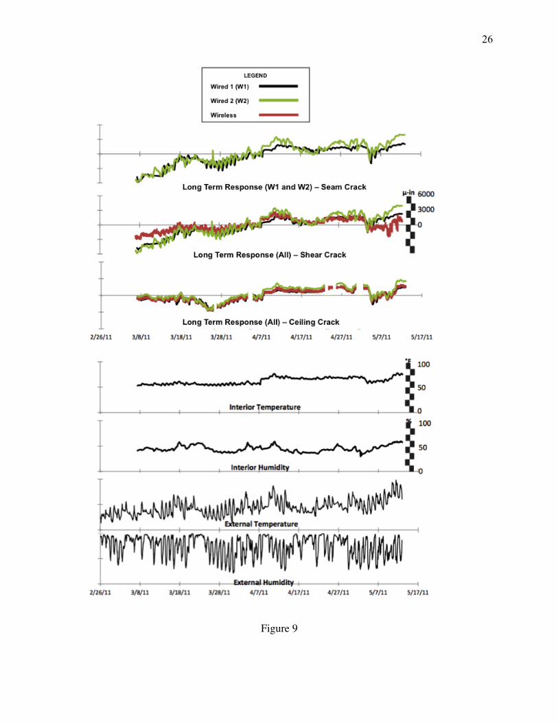
Crack response measurements over a two-month period returned by these three systems 199
are compared in Figure 9. Responses, in micrometers, measured by the three systems are plotted 200
on top of each other for each crack with time along the horizontal axis. These long-term 201
responses are the aggregation of measurements made autonomously every hour by the W1 and 202
W2 and every 15 minutes by the wireless nodes 203
The three systems return the same response over time for the crack in the interior, second 204
floor ceiling. If the crack response is the same at all gage locations, the systems are expected to 205
return the same measurement. This expectation is verified by previous work comparing response 206
of LVDT and potentiometer gages (Ozer, 2005) 207
There is a difference in the responses of the three systems for the shear crack on the south 208
facing exterior wall. The differences occur mainly at the beginning and end of the observation 209
period. Over the two-month observation period, the gage attached to the wireless node responds 210
less than the other two. The W1 LVDT is to the left of the red circle and the node potentiometer 211
and W2 LVDT are in the circle. 212
Detailed fidelity of the wireless system is good on a daily basis as shown by the 213
comparison of the potentiometer response with that of the LVDT response in Figure 10 This 214
figure displays the same information as in Figure 9 only separated and in more detail. In addition 215
to the overall similarity, two areas called out by the vertical lines describe areas that demonstrate 216
fidelity in both long term and daily responses. The daily responses are the oscillations with a 217
return period of one day in the left vertical line and the longer lasting drop on the right is the 218
result of a longer-term climatological influence. 219
While the object of this paper is not a study of crack response, a brief discussion places 220
this study in context. In Figure 9 crack responses (at the top) are compared to the changes in 221

10
exterior and interior temperature and humidity at the bottom. As can be seen, the rise in external 222
temperature beginning in April induces a consistent change in both cracks. This rise in external 223
temperature is accompanied by an increase in interior temperature and humidity. As discussed at 224
length in Dowding (2008), this change in humidity causes the wood in the house to swell and 225
shrink, which induces large changes in crack width. Over the course of these observations, the 226
two cracks changed width by some 75 micrometers several times. In contrast, a quarry blast with 227
peak particle velocities between 5 and 15millimeters per second (mmps) only produced dynamic 228
crack displacements of 1.5 to 3.1 micrometers at the shear crack and 3.1 to 6.4 micrometers at 229
the ceiling crack. This dynamic response is an order of magnitude less than that produced by 230
climatological changes. 231
While this and most wireless system measure long term, climatological crack response 232
well (1 to 4 samples per hour), they cannot measure short term, dynamic response (1000 samples 233
per second) during long time intervals. This generic deficiency is the result of the lack of power 234
provided by batteries small enough to be compatible with the small size of wireless systems. 235
Dynamic events require continuous operation and thus quickly deplete battery power, whereas 236
long term data can be captured by powering up only at selected times, say one can hour. In 237
particular, dynamic events are captured by continuously recording at a high data rate and saving 238
records that contain a data that exceed a threshold. Thus they must continuously record. 239
The long term data, which are measured once an hour, can provide dynamic response 240
information by comparison of before and after blast crack width measures. For instance, a 241
change in the long-term cyclical pattern of crack response after a dynamic event would indicate 242
some change induced by the event. Only changes in pattern are diagnostic. Given the large crack 243
change in crack response shown in Figures 9 & 10 produced by long-term environmental factors 244
during an hour without a dynamic event, these changes would have to be large to be significant. 245
246

11
2) Installation 247
A discussion of the installation differences will be divided into three components: complexity, 248
ease of installation, and cost. Comparison will be based on installation of two similar systems, 249
which differ mainly in their wiring and power, and distribution of sensing activities; the wireless 250
sensor system and the wired W2 .The systems will both monitor 3 crack and null sensors (for a 251
total of 6) and 2 sets of indoor and outdoor temperature and humidity gages (for a total of 4 more 252
and a grand total of 10 channels of data. While the W2 has a greater capability, the comparison 253
will be made on the basis of a need for only 10 channels. As described below the main 254
differences are the lower node costs and lower wiring costs of the wireless system. 255
Complexity can be assessed by considering the sensors, their physical nature and the 256
installation procedure, as well as the integration of the systems with the internet. The attachment 257
process for the displacement transducers is basically the same. While differing slightly in size 258
they both consist of a component glued to the wall on either side of the crack. The sensor output 259
wires for the wireless system only need to be connected to the nearest node, while the sensor 260
output wires for the W2 system need to be strung all the way back to the single, centrally-located 261
W2. Both require an internet connection: the wireless base station and the W2 have standard 262
Ethernet ports with statically or dynamically-assigned IP addresses. The main operational 263
difference in sensor installation between these two systems is the process of zeroing the sensor. 264
The W2’s high sample rate and real-time display capabilities allow sensor zeroing to be 265
completed in under two minutes per sensor.(the time necessary for the glue to cure), whereas the 266
process requires some 10 or more minutes for each sensor connected to a wireless node because 267
of the 15-second data acquisition interval during the first hour after each node is powered on. 268
Ease of installation can be assessed by considering wiring, power, sensor power 269
requirements, and location restrictions. Wired systems can require up to 10 person-hours to run 270
the wires to the sensors, often requiring drilling through walls, while the wireless system wiring 271
12
time is part of the transducer installation. Thus wired systems require some ten hours of 272
additional installation time. Both systems require standard household power. The wired W2and 273
its associated support electronics supply power to the transducers, while the wireless nodes 274
supply transducer power from their own batteries. The wireless nodes should be placed by 275
windows for solar power or if possible supplemented with a panel in a sunny location. This 276
location requirement complicates the placement of the nodes. 277
Finally, cost can be determined by considering the wiring, transducers, data loggers, and 278
internet connection. Research grade instrumentation wire and its associated modular connectors 279
cost approximately $5.00per meter. A typical house could require some 90 meters of 280
instrumentation cable costing some $300 to $500 for a wired W2 system, but less than $100 for 281
the wireless nodes. The transducer costs are similar ~ $200 for each of the displacement 282
transducers or a cost of $2000 for each type of system. The main equipment cost difference is 283
the cost of the systems: A 3 node wireless system with base station might cost ~ $3,500, whereas 284
the W2 system might cost as much as $ 10,000. 285
286
3) Resolution of SHM measurement 287
Resolution of the base mote-based system needed to be improved with the signal conditioner 288
module as introduced in the instrumentation section. This enhancement was needed to increase 289
the resolution of the measurement of crack responses. Since a wireless node has only a 10-bit 290
analog-to-digital converter, it can only divide the measurement range into 210 or 1024 291
subdivisions. Because the excitation voltage is the same as the maximum voltage measureable by 292
the analog-to-digital converter, the mote will always divide the entire 3.8 centimeter range of the 293
potentiometer by 1024, yielding an effective resolution of approximately 0.0025 centimeters 294
The signal conditioner module improves resolution in two ways: it increases the 295
excitation voltage supplied to the potentiometer and it amplifies the output signal from the string 296

13
potentiometer as it is fed back into the mote’s analog-to-digital converter. Because the range of 297
the analog-to-digital converter is not increased, this effectively decreases the range of the sensor 298
by a factor of 10, but also increases the resolution by a factor of 10. Resolution can be further 299
increased, at the expense of total sensor range, by performing hardware modifications to the 300
signal conditioner module. These modifications were not made for this experiment. 301
The effect of the improved resolution is shown in the comparison of the long term 302
response the shear crack (from node 2) before and after installation of the signal conditioner in 303
Figure 11. During similar transitions between heating and cooling seasons (September before 304
and May after) the variability produced by the daily swings is more prominent after the addition 305
of the signal conditioner. 306
307
4) Duration of operation 308
Duration of operation is controlled predominantly by the battery life and ease of recharging. 309
Recharging capability is function of exposure to sun light, and exposure is a complex mixture of 310
location and angle between sun and photovoltaic cells. Locations of nodes 2 and 3 present 311
different exposure environments. Node 3 faces east and generally receives less sunlight than 312
node 2. However, both are shadowed by trees, so the density of the leaves as a function of the 313
season also affects the ability of the nodes to recharge. Figure 11 compares solar voltage and 314
battery voltage for the two nodes. First ignore system failures induced by failure of the base 315
station. Node 3’s battery died (lack of signal after fall in voltage) twice and node 2 only once. All 316
node failures occurred during the summer when the leafy trees shadowed both windows. 317
While not shown here, nodes 4 and 5 (the nodes deployed outdoors and away from 318
trees)did not fail during the one and a quarter year of observation. 319
The base station failures are not related to solar recharging as it operates with 110 v AC 320
power. These failures are a result of long-term instability of the manufacturer-supplied software 321
14
that runs the base station. This instability has been largely improved by upgrades supplied by the 322
manufacturer. 323
324
5) Ease of Operation 325
The wireless node system includes its own graphical display interface, a screen shot of which is 326
shown in Figure 12. As long as the smallest sample interval needed is 15 minutes, this 327
preprogrammed graphical interface can be employed with minimal learning. The crack response 328
as well as the temperature, humidity and battery condition can all be tracked in real time (+/- 15 329
minutes). 330
331
Conclusions 332
This study was undertaken to qualify the use of a wireless “node” system to track crack 333
responses (changes in crack width) to climatological effects. Systems like this can be employed 334
to monitor performance of any component of a constructed facility that involves cracking or 335
relative displacements. Qualification was assessed by comparison of responses of the same crack 336
as measured by the wireless “node” system compared to two wired systems, W2 and W1. In 337
addition the ease and cost of installation of the wireless system was compared with that for the 338
wired W2. The following conclusions were reached within the scope of the comparisons made. 339
Since the wireless, “node” system is typical of such systems, these conclusions can be 340
extrapolated to the class. If better performing equipment were available, it would have been 341
employed. Of course as development continues with the typical speed of digital electronics, one 342
should expect some of the observations to become dated. The wireless “node” system: 343
1) measures the long term crack response as well as the wired system(s), 344
2) has less crack response resolution than does the wired system even if a signal-conditioning 345
unit is installed, 346

15
3) cannot capture dynamic responses directly, but can provide indirect detection if large changes 347
in the cyclic response patterns occur at a time of a dynamic event, 348
4) is easier to install and less complex than wired systems, 349
5) is less costly (half the cost of a wired system), 350
6) operates autonomously as does the wired system, 351
7) graphically displays long term crack responses autonomously over the internet as do wired 352
systems, 353
8) can operate for intervals of time approaching a year provided that the nodes are placed near 354
windows that are not shaded by deciduous trees. 355
356
Acknowledgements 357
The authors are indebted to the research-engineering group of the Infrastructure Technology 358
Institute [ITI] of Northwestern University: Dave Kosnik, Mat Kotowsky, and Dan Marron, as 359
well as Jeff Meissner. We are also grateful for the financial support of ITI for this project 360
through its block grant from the U.S. Department of Transportation to develop and deploy new 361
instrumentation to construct and maintain the transportation infrastructure. Finally we are 362
indebted to Vulcan Materials Corporation for allowing the test house to be instrumented and for 363
sharing portions of the blast data associated with the fragmentation at the adjacent quarry. 364
Without this unique resource this work could not have been undertaken or accomplished. 365
366
References 367
Dowding, C.H. (2008) Micrometer Crack Response to Vibration and Weather, International 368
Society of Explosive Engineers, Cleveland, OH, 409 pgs 369
Koegel, T. (2011) Comparative Report, Internal Report for the Infrastructure Technology 370
Institute, Northwestern University, Evanston, IL. 371
16
Kotowsky, M. (2010) “Wireless Sensor Networks for Monitoring Cracks in Structures”, MS 372
Thesis, Department of Civil Engineering, Northwestern University, Evanston, IL. Also 373
available at www.iti.northwestern.edu/acm under publications. 374
Ozer, H. (2005) “Wireless Crack Measurement for the control of construction vibrations”, MS 375
Thesis, Department of Civil Engineering, Northwestern University, Evanston, IL. . Also 376
available at www.iti.northwestern.edu/acm under publications. 377
Meissner (2010) “Installation report for Sycamore test house” Internal Report for the 378
Infrastructure Technology Institute, Northwestern University, Evanston, IL 379
List of Figures
Figure 1: Instrumented house located just south of the quarry with aerial photograph of the quarry showing the location of the house.
Figure 2: Location of the nodes showing the relation of the instrumented house (nodes, 2 & 3) outdoor nodes (nodes 4 and 5), and the location of the base station (node 0), and node 1 (not deployed).
Figure 3: Installation of exterior nodes. Left installation includes temperature and humidity sensor module below the node.
Figure 4: Plan view of the first and second floors of the test house showing the location of the interior nodes (yellow) Temperature and humidity sensors (red) and crack sensors (green: 1 &2 on south wall and 3 on second floor ceiling).
Figure 5: Context of south wall installation: wireless node on window frame, signal conditioners (black boxes immediately below the node on window frame) on lines leading to sensors (temperature & humidity and crack sensors. Red circle encircles the potentiometer crack sensors attached to wireless node by blue lines. The crack, which transects the upper two displacement sensors in the inset red circle, is underlined by a dashed line.
Figure 6: Context of node 3 and ceiling crack sensor. A close-up photograph of the ceiling crack and potentiometric proximity sensor is shown in Figure 8.
Figure 7 Wireless node weatherproof enclosure and access ports: (Justin Lueker, 2012)
Figure 8: Details of the potentiometric proximity sensor spanning the ceiling crack
Figure 9: Comparison of long-term response of the three systems with temperature and humidity.

17
Figure 10: Comparison of the long-term responses of the shear and ceiling cracks as provided by the W1 and wireless node systems.
Figure 11: Top: Comparison of wireless system’s battery life during one year of operation. Upper graph: Node 2 depletion occurred because of the leaf induced shading of the window in which the node was installed. Middle: Solar voltage shows fluctuations increasing after leaves blossomed. Bottom: Comparison of the crack displacements recorded by the same node before (left) and after (right) addition of the signal conditioning board to amplify the signal.
Figure 12: Preprogrammed graphical users interface supplied by the wireless system’s manufacturer. Data can be either plotted in their raw point form (triangles) or interpolated line form (solid). (Manufacturer’s Users Manual-Meissner, 2010)
18
Figure 1

19
Figure 2

20
Figure 3

21
Figure 4

22
Figure 5

23
Figure 6

24
Figure 7

25
Figure 8
26
Figure 9

27
Figure 10

28
Figure 11

29
Figure 12