2 inferring smart schedules for dumb thermostatslass.cs.umass.edu/papers/pdf/iprogram_tcps.pdf · 2...

2

Inferring Smart Schedules for Dumb Thermostats1

SRINIVASAN IYENGAR, University of Massachusetts AmherstSANDEEP KALRA, University of Massachusetts AmherstANUSHREE GHOSH, University of Massachusetts AmherstDAVID IRWIN, University of Massachusetts AmherstPRASHANT SHENOY, University of Massachusetts AmherstBENJAMIN MARLIN, University of Massachusetts Amherst

Heating, ventilation, and air conditioning (HVAC) accounts for over 50% of a typical home’s energy usage. A thermostatgenerally controls HVAC usage in a home to ensure user comfort. In this paper, we focus on making existing “dumb”programmable thermostats smart by applying energy analytics on smart meter data to infer home occupancy patterns andcompute an optimized thermostat schedule. Utilities with smart meter deployments are capable of immediately applyingour approach, called iProgram, to homes across their customer base. iProgram addresses new challenges in inferring homeoccupancy from smart meter data where i) training data is not available and ii) the thermostat schedule may be misalignedwith occupancy, frequently resulting in high power usage during unoccupied periods. iProgram translates occupancy patternsinferred from opaque smart meter data into a custom schedule for existing types of programmable thermostats, e.g., 1-day,7-day, etc. We implement iProgram as a web service and show that it reduces the mismatch time between the occupancypattern and the thermostat schedule by a median value of 44.28 minutes (out of 100 homes) when compared to a default8am-6pm weekday schedule, with a median deviation of 30.76 minutes off the optimal schedule. Further, iProgram yieldsa daily energy savings of 0.42kWh on average across the 100 homes. Moreover, the schedules generated from iProgramconverge to optimal schedules within a couple of weeks for most homes. We also show that homeowners having multipleHVAC zones can utilize iProgram and potentially increase unconditioned times of less occupied parts of their homes by 70%.Utilities may use iProgram to recommend thermostat schedules to customers and provide them estimates of potential energysavings in their energy bills.

CCS Concepts: •Computer systems organization ! Embedded systems; Redundancy; Robotics; •Networks ! Networkreliability;

ACM Reference Format:ACM Trans. Cyber-Phys. Syst. 9, 10, Article 2 (March 2016), 28 pages.DOI: 0000001.0000001

1. INTRODUCTIONBuildings account for over 40% of the energy and 75% of the electricity usage in the U.S. [Kelso2012] and other developed countries. Heating, cooling and ventilation (HVAC) alone accounts for54% of the energy usage in residential buildings. Thermostats typically regulate use of centralHVAC systems by enabling users to specify a desired setpoint temperature, and then cycling thesystem on and off to maintain the temperature within a fixed range of the setpoint.

The simplest type of thermostat requires users to manually switch the HVAC system on and placeit into heating or cooling mode, as well as specify the desired temperature. Manual thermostats,while simple and inexpensive, are i) prone to human error, since users may forget to turn themoff when leaving for an extended period, and ii) reduce user comfort, since users cannot activatethem in advance of their arrival, causing an initial period of discomfort on entry as a home (orroom) heats up or cools down to the setpoint. To address these drawbacks, most modern thermostats

1preliminary version of this work appeared at the ACM Buildsys 2015 conference.

Permission to make digital or hard copies of all or part of this work for personal or classroom use is granted without feeprovided that copies are not made or distributed for profit or commercial advantage and that copies bear this notice andthe full citation on the first page. Copyrights for components of this work owned by others than ACM must be honored.Abstracting with credit is permitted. To copy otherwise, or republish, to post on servers or to redistribute to lists, requiresprior specific permission and/or a fee. Request permissions from [email protected].© 2016 ACM. 2378-962X/2016/03-ART2 $15.00DOI: 0000001.0000001

ACM Transactions on Cyber-Physical Systems, Vol. 9, No. 10, Article 2, Publication date: March 2016.

2:2

are programmable. A programmable thermostat enables a user to manually program a thermostatschedule, which specifies the time each day the HVAC system should be on and its correspondingsetpoint temperature. Users derive a schedule based on when they expect to be home and away.If a user’s expectations are correct, then a programmable thermostat can reduce human error byautomatically turning off (or adjusting the setpoint) when a user leaves. To increase comfort, usersmay also enter schedules that pre-cool or pre-heat a home (or room) in advance of their expectedarrival.

Programmable thermostats are simple and cheap devices present in tens of millions of homes.While programmable thermostats are marketed for their potential energy savings, prior researchhas shown they do not save energy in practice, largely because users often program them incor-rectly or not at all [Nevius and Pigg 2000; Peffer et al. 2011]. Unfortunately, the interface to manyprogrammable thermostats is difficult to navigate and tedious to program, which often discouragesusers from ever programming them. Even when taking the time to program a schedule, users areleft with the complex task of determining a static schedule that optimizes their energy savings andcomfort given their occupancy pattern, which may be dynamic and difficult to predict. Further, sincedaily activities and, thus, occupancy patterns inevitably change over time, e.g., summer activitiesdiffer from winter activities, users must periodically re-program their thermostat as their optimalschedule changes, or risk losing any of its energy-saving benefits. As a result of these challenges,many users avoid programming thermostats, which defeats their purpose.

Smart thermostats, which sense occupancy and automatically program a schedule without userintervention, were introduced to address the drawbacks of programmable thermostats. There hasbeen a large amount of prior work on smart thermostats that monitor and predict occupancy patternsusing various techniques and sensors, e.g., motion or GPS [Agarwal et al. 2011; Erickson et al.2011; Erickson and Cerpa 2010; Lu et al. 2010; Scott et al. 2011], and numerous commercial smartthermostats are now available, including NEST [nest 2015], Lyric [lyric 2015], Ecobee [ecobee2015], etc. However, smart thermostats are still niche devices for energy-efficiency enthusiasts,largely due to their high cost and the overhead of installing them. For example, smart thermostatscurrently cost >10⇥ more than a programmable thermostat, e.g., $250 for the NEST versus $15 orless for an entry-level programmable thermostat. While the cost of smart thermostats may decreaseover time, tens of millions of “dumb” programmable thermostats will remain in homes for manyyears to come.

Thus, we focus on making existing “dumb” programmable thermostats smart without requiringnew investments to upgrade to an expensive smart thermostat or install additional sensors. Our goalis to address the problems that prevent existing programmable thermostats from fully realizing theirenergy savings potential. Our key insight is that electricity usage data from smart meters indirectlyreveals occupancy patterns that can be used to automatically derive custom thermostat schedules foreach home. We argue that schedules automatically derived from smart meter data are better alignedwith occupancy than schedules manually entered by users, enabling users to save energy and mak-ing it easier for them to program their thermostat. Importantly, our approach uses an existing sensorthat is already widely deployed in homes: as of 2014, 50 million smart meters had been installed inthe U.S., which covers more than 43% of all meters [John 2014]. Further, smart meter installationsare growing rapidly: in the past five years from 2009 to 2014 the number of deployments increasedby nearly a factor of four (from 13 million in 2009 to 50 million in 2014 [John 2014]) with 75%coverage expected by 2016 [Fehrenbacher 2012]. In addition, utilities that collect smart meter datahave an interest in energy-efficiency, e.g., as part of government-mandated energy-efficiency pro-grams, and direct access to a large set of customers and data. Thus, utilities are in the best positionto suggest thermostat schedules to users, to provide incentives for users to adopt them, and to verifytheir adoption.

Our system, called iProgram, analyzes data from a home’s smart electricity meter to infer occu-pancy patterns and derive a custom thermostat schedule. iProgram extends recent research [Chenet al. 2013; Kleiminger et al. 2013] in inferring occupancy from smart meter data in important ways,which are driven by its application context. For example, while prior work uses training data to build


2:3

a model that correlates occupancy with certain features of smart meter data [Kleiminger et al. 2013],our application does not permit gathering training data, since it would require installing temporaryoccupancy sensors in tens of millions of homes. In addition, the models in prior work typically usea home’s power usage as primary feature to infer occupancy. Unfortunately, homes with mispro-grammed thermostats often exhibit high power usage when unoccupied, since the HVAC system isoften a home’s largest load. Thus, prior techniques often perform poorly on exactly the homes withthe most to gain from iProgram. Finally, we evaluate iProgram, not only using occupancy-centricaccuracy metrics, but also by its ability to derive effective thermostat schedules in real homes.

Our hypothesis is that iProgram can improve HVAC efficiency en masse by analyzing smart meterdata to infer long-term occupancy patterns and compute a custom thermostat schedule. In evaluatingour hypothesis, this paper makes the following contributions.

• Targeted Occupancy Detection. We develop a targeted occupancy detection technique thatperforms well on energy-inefficient homes with misprogrammed thermostats, and is applica-ble to utility-scale datasets where training data is not available. Rather than apply a generalmachine learning approach, we craft a domain-specific technique that leverages time-seriescomponent analysis to isolate the “burstiness” of interactive loads that directly correlate withoccupancy. Occupancy for individual zones in house can also be inferred.Deriving Thermostat Schedules. We show how to translate the inferred long-term occupancypatterns into a probability distribution of occupancy to derive a custom static thermostat sched-ule. We present extensions to support scheduling different types of thermostats, e.g., 5-2-day,7-day, etc., identifying sleeping periods, and changing occupancy patterns. Further, we discussa Manhattan distance-based approach to reduce the frequency of re-deriving custom scheduleswith increased availability of smart meter data.Open Cloud Service. We implement iProgram as an open cloud service where users mayupload their smart meter data and receive suggested thermostat-specific schedules. The servicealso exposes a web services API to enable third-party devices, such as a basic WiFi-enabled(but non-learning) programmable thermostat, to access its schedules.Evaluation. We evaluate the accuracy of iProgram’s targeted occupancy detection techniqueand its derived thermostat schedules, as well as its ability to infer thermostat schedules in realhomes. For the former, we use data from over 100 homes from the ECO [Beckel et al. 2014;Kleiminger et al. 2013] and Pecan Street datasets [pecan 2015], which include one-minutepower data for up to six months. For the latter, we conduct an anonymous user study on 8homes where we analyze their smart meter data to suggest a thermostat schedule based ontheir inferred occupancy pattern. Further, we discuss the efficiency of iProgram to quicklyconverge to a static schedules. Also, we present a case study where we leverage informationfrom additional sensors to improve schedules.

2. BACKGROUND AND MOTIVATIONiProgram assumes a home is equipped with a networked power meter—a smart meter—that reportsaggregate electricity usage at fine-grained intervals, e.g., every one to fifteen minutes. Most residen-tial HVAC systems are partially or fully electric: nearly all space cooling, i.e., air conditioning, iselectric and 38.1% of U.S. homes use some form of electric space heating [eia 2009]. Even whenusing oil- or natural gas-based heating, the mechanical systems that circulate the hot air or water areelectric. In addition, the type of HVAC system in a home is typically a matter of public record, andavailable to iProgram (and utilities). Thus, given an address, iProgram can identify the homes andseasons where HVAC usage is included in smart meter data, and appropriately configure itself.

iProgram specifically targets homes that use programmable thermostats to regulate HVAC oper-ation. Only 7% of U.S. homes have central heating but no thermostat, and only 1% of homes havecentral cooling but no thermostat [eia 2014]. In contrast, 37% of U.S. homes with central heatinghave a programmable thermostat, and 29% of homes with central cooling have a programmablethermostat [eia 2014]. Importantly, iProgram does not dictate a specific type of programmablethermostat or its configuration. There are a wide range of thermostats available, including 1-day


2:4

programmable, 7-day programmable, and 5-2-day programmable. In addition, some programmablethermostats are now networked, enabling users (or third-party software) to remotely program andcontrol them. Note that network-enabled programmable thermostats differ from high-end smart ther-mostats in that they do not automatically program a schedule by learning home occupancy patternsvia sensors.2

For homes with only manual thermostats (or no thermostat at all), iProgram can still compute themisalignment between the HVAC system’s operation and the occupancy pattern, and then estimatethe potential energy savings from upgrading to a programmable (or smart) thermostat.

2.1. Problem StatementOur goal is to analyze a home’s smart meter data to derive a thermostat schedule that accuratelyreflect its pattern of occupancy. Formally, we represent a schedule as a function S(t) that returns adesired thermostat setpoint temperature at each time t. In essence, the thermostat schedule definedby S(t) consists of a series of variable-length intervals that specify different setpoint and setbacktemperatures, which denote the desired temperature when users are present and away, respectively.A thermostat schedule must specify either a setpoint or setback temperature for each interval. Inaddition, for programmable thermostats, the thermostat schedule repeats every interval T , whichlimits t’s range. For example, for a 1-day programmable thermostat T = 24 hours, while, for a7-day programmable thermostat, T = 168 hours.

iProgram derives the schedule S(t) by analyzing the time-series P (t) of power readings generatedby a smart meter to infer when a home is occupied. As in prior work, we represent occupancy as abinary function O(t), where zero is an unoccupied home and one is an occupied home. Occupancydetection then requires inferring O(t) from P (t). Prior work on inferring occupancy from smartmeter data leverages the insight that power usage that is high and variable often correlates withoccupancy, since occupants use interactive devices that consume energy when home. Prior workevaluates many approaches for inferring occupancy based on this intuition, ranging from employingsimple thresholds on power’s mean, variance, and range [Chen et al. 2013] to advanced machinelearning techniques using Hidden Markov Models (HMMs), Support Vector Machines (SVMs),and k-Nearest Neighbor (k-NN) classifiers [Kleiminger et al. 2013]. While accuracy depends on thecorrelation between a home’s occupancy and electricity usage, it generally ranges between 75% and95%.

2.2. Research ChallengesUnfortunately, applying prior work to iProgram’s application of deriving optimal thermostat sched-ules en masse from smart meter data is problematic for multiple reasons. As we describe below,iProgram i) does not have access to training data, ii) has a particular emphasis on reducing the en-ergy use of energy-inefficient homes with misprogrammed thermostats, and iii) focuses on derivingthermostat schedules and not just detecting occupancy.No Training Data. Prior techniques for inferring occupancy from smart meter data rely on an initialset of training data to build a model that correlates occupancy with power data. Gathering trainingdata requires instrumenting the home with occupancy sensors or directly tracking occupants’ loca-tion, e.g., via their smartphone. While gathering training data is feasible in a few homes, it doesnot scale to utility-sized datasets. Further, many users will not likely consent to such instrumenta-tion due to privacy concerns. While improving home thermostat schedules across a large number ofhomes has the potential to significantly reduce energy use, the cost to privacy may not be worth thebenefit in energy savings for many users. While privacy concerns also exist with smart meters [Chenet al. 2014], consumers must already trust utilities with their smart meter data.

Of course, one way to address the lack of training data using the techniques above is to sim-ply apply models built from training data from some sample test homes to a much larger set ofhomes. Other energy data analytics, such as Non-Intrusive Load Monitoring (NILM), often take

2See http://wifithermostat.com for examples.


2:5

12 AM 4 AM 8 AM 12 PM 4 PM 8PM 12 AMTime

0.0

0.5

1.0

1.5

2.0

2.5

3.0

3.5

Pow

er(k

Wh)

Misaligned AC

Ground truth Occupancy Inferred Occupancy

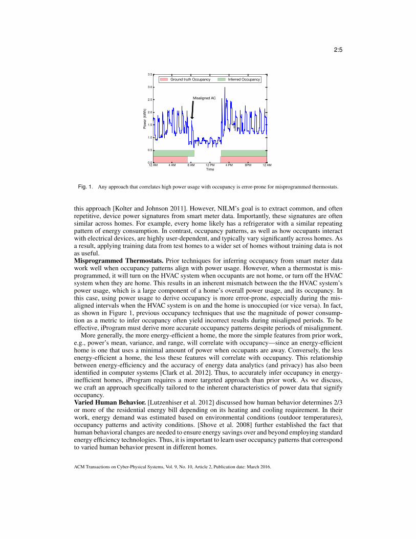
Fig. 1. Any approach that correlates high power usage with occupancy is error-prone for misprogrammed thermostats.

this approach [Kolter and Johnson 2011]. However, NILM’s goal is to extract common, and oftenrepetitive, device power signatures from smart meter data. Importantly, these signatures are oftensimilar across homes. For example, every home likely has a refrigerator with a similar repeatingpattern of energy consumption. In contrast, occupancy patterns, as well as how occupants interactwith electrical devices, are highly user-dependent, and typically vary significantly across homes. Asa result, applying training data from test homes to a wider set of homes without training data is notas useful.Misprogrammed Thermostats. Prior techniques for inferring occupancy from smart meter datawork well when occupancy patterns align with power usage. However, when a thermostat is mis-programmed, it will turn on the HVAC system when occupants are not home, or turn off the HVACsystem when they are home. This results in an inherent mismatch between the the HVAC system’spower usage, which is a large component of a home’s overall power usage, and its occupancy. Inthis case, using power usage to derive occupancy is more error-prone, especially during the mis-aligned intervals when the HVAC system is on and the home is unoccupied (or vice versa). In fact,as shown in Figure 1, previous occupancy techniques that use the magnitude of power consump-tion as a metric to infer occupancy often yield incorrect results during misaligned periods. To beeffective, iProgram must derive more accurate occupancy patterns despite periods of misalignment.

More generally, the more energy-efficient a home, the more the simple features from prior work,e.g., power’s mean, variance, and range, will correlate with occupancy—since an energy-efficienthome is one that uses a minimal amount of power when occupants are away. Conversely, the lessenergy-efficient a home, the less these features will correlate with occupancy. This relationshipbetween energy-efficiency and the accuracy of energy data analytics (and privacy) has also beenidentified in computer systems [Clark et al. 2012]. Thus, to accurately infer occupancy in energy-inefficient homes, iProgram requires a more targeted approach than prior work. As we discuss,we craft an approach specifically tailored to the inherent characteristics of power data that signifyoccupancy.Varied Human Behavior. [Lutzenhiser et al. 2012] discussed how human behavior determines 2/3or more of the residential energy bill depending on its heating and cooling requirement. In theirwork, energy demand was estimated based on environmental conditions (outdoor temperatures),occupancy patterns and activity conditions. [Shove et al. 2008] further established the fact thathuman behavioral changes are needed to ensure energy savings over and beyond employing standardenergy efficiency technologies. Thus, it is important to learn user occupancy patterns that correspondto varied human behavior present in different homes.


2:6

Thermostat Scheduling. There is substantial work on deriving thermostat schedules from occu-pancy patterns. For example, smart thermostats actively sense occupancy using motion or GPSsensors [Lu et al. 2010; Scott et al. 2011] and dynamically alter a thermostat’s schedule in realtime based on the current occupancy. The scheduling problem for iProgram differs from smartthermostats, since it computes a static schedule based on long-term occupancy patterns for a pro-grammable thermostat, rather than directly sensing and dynamically adjusting to real-time occu-pancy. Work by Gao and Whitehouse [Gao and Whitehouse 2009], which computes a thermostatschedule based on long-term occupancy statistics gathered from sensors, is most similar to iPro-gram’s scheduling problem. However, their approach is limited to computing the time and durationof a single unoccupied period each day, while our approach is general and computes the optimalthermostat schedule for a given long-term pattern of occupancy.Faster convergence to a static schedule. As discussed earlier, Gao and Whitehouse [Gao andWhitehouse 2009] presented a technique that derives thermostat schedules from occupancy patterns.However, the amount of occupancy data required to achieve a static schedule is not discussed. Forapplicability of iProgram or any other technique that derives custom schedules from occupancy datamust quickly converge to a static schedule so as to benefit the residents immediately. For example,a house with a fairly stable schedule must be able to leverage custom schedules generated fromiProgram that is reasonably accurate. In this paper, we present empirical convergence results of ourschedules derived from occupancy data.Schedule change adoption. Homes might have a changed occupancy pattern for a plethora ofreasons — summer vacation in schools, change of shift for the working residents etc. Thus, theschedules generated must be updated to reflect the changes in schedules. One can either do thisperiodically, say once every week/month, or dynamically by observing the changes in the occupancypattern. Constantly, changing the custom schedules generated might not be necessary. Deciding onwhen or how often to re-derive custom schedules should be governed by the significant changeobserved in occupancy patterns.

2.3. Evaluation MetricsSince iProgram ultimately focuses on translating occupancy patterns into a thermostat schedule,we use evaluation metrics relevant to thermostat scheduling, rather than simply quantifying theaccuracy of our new binary classifier for occupancy detection. In particular, we use miss time (MT)and waste time (WT) to quantify the performance of a thermostat schedule. Intuitively, the miss timeis the amount of time a home is occupied but the HVAC system is not on, i.e., where its temperaturedeviates by more than X� from the setpoint. Likewise, the waste time is the amount of time a homeis unoccupied and the HVAC system is on, i.e., where the temperature deviates by less than X� fromthe setpoint. Formally, we define the miss time and waste time in terms of the conditioning period(CP) below for T time periods with occupancy O(t) 2 0, 1.

CP (t) =

⇢1, if the home is conditioned at time t,0, otherwise.

(1)

Given CP(t), we define the average daily miss time and waste time over an N day period, asshown below.

MT =

Pt

(O(t)� CP (t))

N8 t where O(t) = 1 (2)

WT =

Pt

(CP (t)�O(t))

N8 t where CP (t) = 1 (3)


2:7

Our definition of miss time differs from prior work [Gao and Whitehouse 2009], which definedthe metric by assuming only a single contiguous unoccupied period during the day, e.g., from thetime occupants leave in the morning to when they return in the afternoon/evening. In general, ourmetric reflects that there may be multiple non-contiguous unoccupied periods during the day, e.g.,if someone leaves for work, comes home for lunch, and then leaves again. Our definition of misstime is applicable to such non-contiguous schedules.

Of course, a simple way to achieve a miss time of zero is to never alter the thermostat setpoint,even when a home is not occupied; likewise, a simple way to achieve a waste time of zero is tonever turn on the HVAC system, even when the home is occupied. There is a tradeoff betweenmiss time and waste time, which corresponds to a tradeoff between user comfort and HVAC energyusage: a low miss time signifies high user comfort but results in higher HVAC energy usage, whilea low waste time signifies low HVAC energy usage but results in lower user comfort. To resolvethis tradeoff, we also define the mismatch time for a particular schedule as the sum of its miss timeand waste time. The mismatch time essentially places an equal value on both energy-efficiency andcomfort.

Note that iProgram computes a thermostat schedule S(t) for homes that specifies when the ther-mostat should be at a setpoint or a setback temperature. However, it does not determine the setpointand setback temperature for the user. These values should be defined by a home’s occupants, sincethey depend on occupants’ subjective notion of comfort, i.e., some people may like their homewarmer or colder than others. iProgram could aid in setting setback temperatures based on the reg-ularity and length of a home’s occupancy pattern. For example, the more regular and predictable ahome’s schedule, the deeper the setback that is possible without causing discomfort on arrival (sincethe schedule will be able to reliably pre-heat the home before the expected arrival). In addition, set-ting the depth of the setback also depends on a home’s size and insulation, since these attributesaffect the time it takes to change the temperature back to the setpoint temperature. We leave settingthe setback temperature’s depth as future work: in our current prototype, iProgram computes theschedule, while the user sets their desired setpoint and setback temperature for different periods.

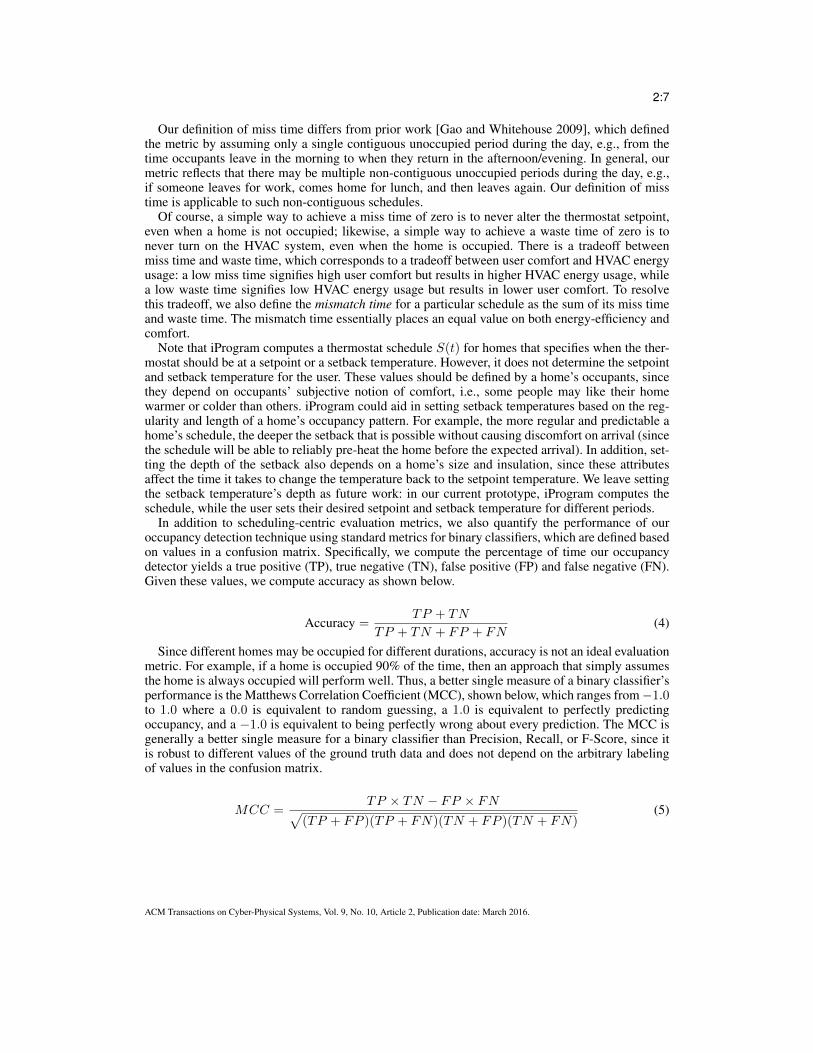
In addition to scheduling-centric evaluation metrics, we also quantify the performance of ouroccupancy detection technique using standard metrics for binary classifiers, which are defined basedon values in a confusion matrix. Specifically, we compute the percentage of time our occupancydetector yields a true positive (TP), true negative (TN), false positive (FP) and false negative (FN).Given these values, we compute accuracy as shown below.

Accuracy =TP + TN

TP + TN + FP + FN(4)

Since different homes may be occupied for different durations, accuracy is not an ideal evaluationmetric. For example, if a home is occupied 90% of the time, then an approach that simply assumesthe home is always occupied will perform well. Thus, a better single measure of a binary classifier’sperformance is the Matthews Correlation Coefficient (MCC), shown below, which ranges from�1.0to 1.0 where a 0.0 is equivalent to random guessing, a 1.0 is equivalent to perfectly predictingoccupancy, and a �1.0 is equivalent to being perfectly wrong about every prediction. The MCC isgenerally a better single measure for a binary classifier than Precision, Recall, or F-Score, since itis robust to different values of the ground truth data and does not depend on the arbitrary labelingof values in the confusion matrix.

MCC =TP ⇥ TN � FP ⇥ FNp

(TP + FP )(TP + FN)(TN + FP )(TN + FN)(5)


2:8

Occupancy(Detec,on( Probability(Quan,fica,on( Schedule(Genera,on(

Fig. 2. iProgram’s basic workflow

3. IPROGRAM DESIGNiProgram’s basic workflow, depicted in Figure 2, is to i) apply an occupancy detection techniqueto infer occupancy from smart meter data, ii) use the inferred long-term occupancy pattern tocompute a histogram of the probability of occupancy at any time each day, and iii) generate astatic schedule that minimizes the mismatch time (or optimizes a user-specified tradeoff betweenmiss time and waste time). Since prior general occupancy detection techniques [Chen et al. 2013;Kleiminger et al. 2013] do not work well for iProgram, as discussed in Section 2, we present a newtargeted technique designed specifically to work without training data on energy-inefficient homeswith misprogrammed thermostats. We then discuss translating the inferred occupancy patterns intonon-contiguous schedules for programmable thermostats. Our techniques combine several statisticalmethods, including time-series decomposition and probability-based occupancy modeling, to derivecustom thermostat schedules. In addition, we present multiple extensions to our basic technique.

3.1. Detecting OccupancyOur approach derives from the notion of “burstiness” in network protocols, such as TCP [Shakkottaiand Brownlee 2005]. A TCP flow consists of a sequence of packets from a source to a destinationserver. Intuitively, a burst is then a group of consecutive packets with shorter inter-arrival times thanpackets occurring before or after the group. In addition, a group of bursts with shorter inter-arrivaltimes than bursts occurring before or after the group is referred to as a family of bursts.

In our context, packets are analogous to significant power events, i.e., increases or decreases inpower. We apply burstiness to occupancy detection, in part, because we view it as the most innatecharacteristic of power usage that directly correlates with occupancy: when occupants are home theycause bursts of power events by turning devices on and off. Other characteristics of home powerusage that correlate with occupancy, including power’s mean, variance, and range, only indirectlyderive from burstiness. For example, power’s mean tends to increase as occupants turn devices on.Likewise, power’s variance (or standard deviation) is essentially a dampened form of burstiness,while power’s absolute range simply captures the largest burst within some period.

Since the characteristics above are not the most direct reflection of occupant presence in smartmeter data, their correlation with occupancy is generally less strong than burstiness. As discussed inSection 2, any technique that correlates occupancy with a high average power will incorrectly detectoccupancy if the HVAC system turns on in an unoccupied home.

Of course, burstiness, as with the other metrics, may not always perfectly correlate with oc-cupancy, as large background loads like the HVAC system also cause bursts of power events. Toisolate these bursts, we use basic time-series decomposition to deconstruct the power time series(P ) into the seasonal(P

s

), trend(Pt

), and noise (Pn

) components. The seasonal component of a timeseries captures patterns that tend to repeat semi-regularly over known, fixed periods of time (of anyduration). Thus, the seasonal component only includes the non-interactive background loads, whichare typically periodic and cause bursts of power usage in an unoccupied home. In contrast, the trendcomponent captures the general non-repetitive trend in the data, e.g., increasing or decreasing overtime, by filtering out medium and high frequency fluctuations. Thus, in our algorithm below, weonly correlate bursts in the power usage of the trend component with occupancy. Finally, the noisecomponent represents random fluctuations that are neither repetitive nor follow a trend. We extractthe noise component from the trend component to eliminate random bursts that are less likely to beassociated with human activity, which are generally part of a trend.


2:9

Below, we present our occupancy detection algorithm that combines time-series decompositionand burstiness to detect occupancy from smart meter data. For each day, from time dStart to timedEnd, we isolate the periodic background loads using time-series decomposition. Specifically, wecompute the seasonal component of the daily time-series for all window sizes [1 . . . ⌫

max

], and thenselect the value ⌫

opt

that maximizes the seasonal component’s average power consumption over theday. Here, the time-series decomposition will extract any repeating patterns of usage that are nearthe specified window size. Our goal is to isolate the HVAC system’s operation from the power usage;since the HVAC system is generally the largest load in the home, computing the seasonal componentat its window size, i.e., its periodic interval, will result in the largest energy consumption over theday. Since we do not know the HVAC system’s duty cycle and periodicity in advance, we performan exhaustive search over all possible window sizes.

Algorithm 1 Occupancy Detection1: procedure OCCUPANCYDETECTION(P )2: Initialize: O[i] 0 8 i 2 1 . . . length(P )3: P

day

P [dStart : dEnd]4: P

s

[⌫], Pt

[⌫], , Pn

[⌫] Decompose(Pday

, ⌫)8 ⌫ 2 1 . . . ⌫

max

5: ⌫opt argmax⌫

|�(Ps

[⌫])|

6: P opt

s

, P opt

t

, P opt

n

Decompose(Pday

, ⌫opt)7: O

day

(O1[Popt

t

]| > mean(|O1[Popt

t

]|))8: O

day

[i : i+ 1] 1 8 T (i+ 1)� T (i) <= �day

9: Onight

[i] Oday

[i] 8 i 2 T [nStart : nEnd]10: O

night

[i : i+ 1] 1 8 T (i+ 1)� T (i) <= �night

11: O[i] 1 8 i 2 Oday

[i] = 112: O[i] 1 8 i 2 O

night

[i] = 113: return O14: end procedure

After isolating the seasonal component with the window size that maximizes daily energy con-sumption, we consider the magnitude of the change in the trend component over time. In particular,if the change in the power usage of the trend component from any time t � 1 to time t is greaterthan the average reading-to-reading change in power, we flag time t as a power event. If the timeperiod between two events is within a threshold �

day

, we label the time period between the eventsas a burst. Similarly, if the time period between two bursts is within a threshold �

day

, we label thetime period between the bursts as a family of bursts. We set �

day

= 2 hours in our current prototype.We then interpolate between families of bursts and label periods between them as being occupied,while all other periods are labeled as non-occupied. Note that the algorithm above only considersdaytime detection from 6am to 11pm.

We detect nighttime occupancy separately from daytime occupancy, since nighttime occupancy isnot strongly correlated with burstiness in the power usage. Here, we focus on evening and morningbursts that occur between 7pm-11pm and 6am-9am, respectively. If we do not detect a burst in eitherperiod, we label the nighttime period as unoccupied, otherwise we compute occupancy as above.The choice of fixing the periods (6-9am, 7-11pm) is made to capture the most common energy usagepatterns i.e. load profiles observed in the residential setting. Typical residential homes have a spurt inenergy usage in the morning and one during the evening. [Iyengar et al. 2016] presented an analysisof a New England city's gas and electric data which provided insights into the energy consumption ofresidential homes. According to the analysis mentioned in this work, 10475 out of 11431 residentialhomes (⇡ 92%) have increased energy consumption during these periods compared to the rest ofthe day.


2:10

12 AM 4 AM 8 AM 12 PM 4 PM 8PM 12 AMTime (minutes)

0.0

0.2

0.4

0.6

0.8

1.0

1.2

Pro

babi

lity

True Occupancy Inferred Occupancy

Fig. 3. An example histogram of the probability of occupancy (inferred and ground truth) each minute of the day over athree week period for Home B in the Smart* dataset [Barker et al. 2012].

The strategy of observering these periods works well in practice, although it cannot differentiatebetween occupants going to sleep and then waking up in the middle of the night, and occupantsgoing out late at night and then coming home in the early morning hours. Pseudocode for ouralgorithm above is shown in Algorithm 1. Further, note that burst detection above is based on themagnitude of each change in power relative to the average reading-to-reading change in power fora home. Thus, the algorithm requires no training data of ground truth occupancy to learn a model apriori. We select the average change in power as the threshold because we have found that changesin home power are bimodal with many small changes in power (near zero) that stem from naturalvariations in a device’s power usage, and a few large changes in power that stem from humanactivity. In computing the mean change in power, we are able to detect the latter, while eliminatingthe former.

3.1.1. Deriving occupancy for different zones in a house. Many homes have multiple thermostatscorresponding to HVAC units dedicated to different parts of the home. These isolated parts of thehome are called zones. Zoning might be extremely beneficial as different parts of the house are notequally occupied. Thus, even when occupants are present at home, part of the home can remain un-conditioned to save energy. To handle this case, we employ the algorithm described above separatelyfor the different zones provided we have submetered energy data.

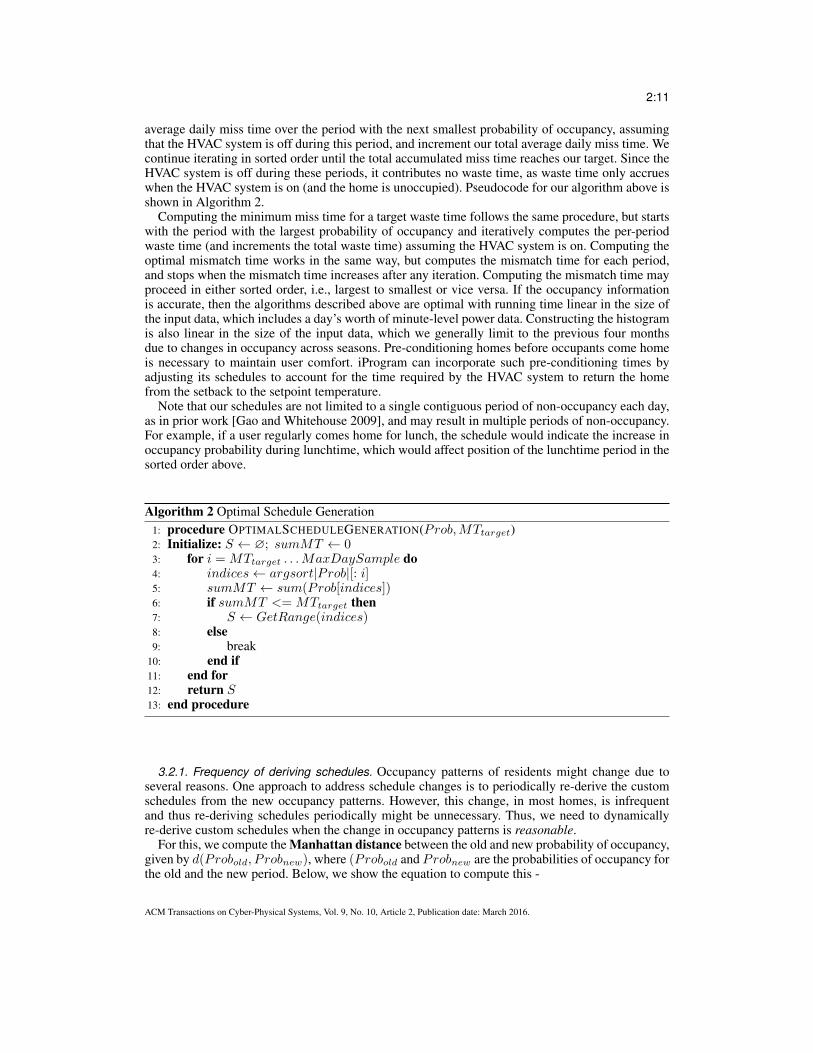
3.2. Generating SchedulesThe algorithm above infers periods of occupancy and non-occupancy each day. Over many days, wecan then compute a histogram that shows the probability of occupancy for each sampling interval,e.g., every minute in our dataset. The histogram captures the regularity of a home’s occupancypattern. Figure 3 shows an example of the histogram for Home B in the UMass Smart* datasetover a three week period. The figure shows the probability the home is occupied each minute of theday for both the ground truth occupancy and our inferred occupancy. For this home, our occupancydetection technique works well, and the home has a highly regular pattern of usage, making it agood candidate for a static thermostat schedule. Using this histogram, we can directly compute aschedule that optimizes for a specific miss time, waste time, or mismatch time. For example, we canspecify a miss or waste time, and compute the schedule that minimizes the waste and miss time,respectively. We can also compute the schedule that minimizes mismatch time, i.e., the sum of missand waste time.

The basic algorithm sorts the histogram by the probability of occupancy for each given time pe-riod. We may then specify a target average daily miss time and compute the schedule that minimizesthe waste time. We start with the period with the lowest probability of occupancy and compute aver-age miss time over this period assuming that we turn off the HVAC system (or shift it to the setbacktemperature). We can compute the average daily miss time directly from the histogram by simplymultiplying the length of the time period by the probability of occupancy. We then compute the


2:11

average daily miss time over the period with the next smallest probability of occupancy, assumingthat the HVAC system is off during this period, and increment our total average daily miss time. Wecontinue iterating in sorted order until the total accumulated miss time reaches our target. Since theHVAC system is off during these periods, it contributes no waste time, as waste time only accrueswhen the HVAC system is on (and the home is unoccupied). Pseudocode for our algorithm above isshown in Algorithm 2.

Computing the minimum miss time for a target waste time follows the same procedure, but startswith the period with the largest probability of occupancy and iteratively computes the per-periodwaste time (and increments the total waste time) assuming the HVAC system is on. Computing theoptimal mismatch time works in the same way, but computes the mismatch time for each period,and stops when the mismatch time increases after any iteration. Computing the mismatch time mayproceed in either sorted order, i.e., largest to smallest or vice versa. If the occupancy informationis accurate, then the algorithms described above are optimal with running time linear in the size ofthe input data, which includes a day’s worth of minute-level power data. Constructing the histogramis also linear in the size of the input data, which we generally limit to the previous four monthsdue to changes in occupancy across seasons. Pre-conditioning homes before occupants come homeis necessary to maintain user comfort. iProgram can incorporate such pre-conditioning times byadjusting its schedules to account for the time required by the HVAC system to return the homefrom the setback to the setpoint temperature.

Note that our schedules are not limited to a single contiguous period of non-occupancy each day,as in prior work [Gao and Whitehouse 2009], and may result in multiple periods of non-occupancy.For example, if a user regularly comes home for lunch, the schedule would indicate the increase inoccupancy probability during lunchtime, which would affect position of the lunchtime period in thesorted order above.

Algorithm 2 Optimal Schedule Generation1: procedure OPTIMALSCHEDULEGENERATION(Prob,MT

target

)2: Initialize: S ?; sumMT 03: for i = MT

target

. . .MaxDaySample do4: indices argsort|Prob|[: i]5: sumMT sum(Prob[indices])6: if sumMT <= MT

target

then7: S GetRange(indices)8: else9: break

10: end if11: end for12: return S13: end procedure

3.2.1. Frequency of deriving schedules. Occupancy patterns of residents might change due toseveral reasons. One approach to address schedule changes is to periodically re-derive the customschedules from the new occupancy patterns. However, this change, in most homes, is infrequentand thus re-deriving schedules periodically might be unnecessary. Thus, we need to dynamicallyre-derive custom schedules when the change in occupancy patterns is reasonable.

For this, we compute the Manhattan distance between the old and new probability of occupancy,given by d(Prob

old

, P robnew

), where (Probold

and Probnew

are the probabilities of occupancy forthe old and the new period. Below, we show the equation to compute this -


2:12

d(Probold

, P robnew

) =TX

t=1

|Probold

(t)� Probnew

(t)| (6)

Using this, we can trigger the schedule generation algorithm, when the Manhattan distance be-tween the old and new probability of occupancy is greater than a pre-defined threshold. The distancemeasure directly maps to the mismatch time between old and the new occupancy pattern.

3.3. Scheduling ExtensionsWe extend iProgram’s basic algorithm in multiple ways.Different Thermostat Types. We can use the same algorithm as above to compute schedules fordifferent types of programmable thermostats, such as 5-2-day or 7-day, by simply considering differ-ent datasets. For a 7-day thermostat, we run the algorithm separately for datasets with all Mondays,all Tuesdays, etc. to compute a separate Monday schedule, Tuesday schedule, etc. Likewise, for a 5-2-day thermostat, we partition the data into two sets—for weekdays and weekends—and separatelycompute schedules for each.Sleeping Schedules. iProgram may also separate sleeping from non-occupancy in its schedules.The sleeping period differs from non-occupancy in that homes may have a different thermostatsetting when the home is occupied and sleeping versus not occupied. For example, homes may setbedroom heating or cooling zones in multi-zoned systems based only on the sleeping versus notsleeping periods, irrespective of occupancy (since bedrooms may not be occupied during the day,even when the home is occupied). iProgram assumes the sleeping period is the longest period ofnighttime occupancy (between 7pm and 9am).Dynamic Learning. Our algorithm above computes static thermostat schedules for different typesof programmable thermostats. However, schedules may change over time. For example, homes’ pat-tern of occupancy generally changes with each season due to changes in the climate or based on theacademic calendar, i.e., children are out of school over the summer. We have extended our approachabove to be more dynamic by recomputing schedules based on new data. In our case, we use amoving average approach that gives more weight to more recent data. To do so, we recompute thehistogram above each day using a weighted measure of occupancy that discounts older occupancydata. One can apply this discount on a monthly basis, since we are primarily focused on adapting toseasonal changes. Thus, to compute the histogram, we give full weight to occupancy data within thepast month, and discount older data by a factor ↵ < 1. While a recomputed schedule would needto be manually (re)programmed by the user, which implies it should be infrequent and only capturelarge changes in the schedule, the process may be automated for newer programmable thermostatswith WiFi capabilities.Feedback Module. Further, we have added a human feedback module, which can correct any per-sonal occupancy quirks such as occupancy with low human activity. If iProgram incorrectly classi-fies an occupied period as unoccupied, the human feedback is recorded when the users manually setthe thermostat. Later, this is used in the occupancy detection algorithm as occupied period and theschedules are recomputed to reflect this change for future periods. The above described dynamiclearning component helps in quickly converging to the new schedule.

4. IPROGRAM IMPLEMENTATION4.1. Energy Consumption Data CollectionEnergy consumption data is available to the customers through various interfaces (ranging frompaper bills to custom online utility web portals) and at different granularity (⇡1 min to 1 month).This presents a significant challenge to a 3rd party application, such as iProgram, to collect andanalyze energy usage data. Thanks to DoE’s GreenButton3 initiative increasing number of utilities

3http://www.greenbuttondata.org


2:13

(a) (b)

Fig. 4. iProgram screenshots, including the inferred occupancy (a) and generated thermostat-specific schedule (b).

are making the energy data available in a standard XML format. This allows 3rd party applicationsto assimilate energy consumption patterns at higher granularity (5 min interval). Similarly, popularenergy monitoring devices such as eGauge4 provide a REST API to query either historical or real-time energy data. Moreover, the data from these sources are curated and are in a standard format,which eliminates the pre-processing overheads.

4.2. Handling Missing ValuesThe energy consumption data from smart meters can suffer from measurement error or missingvalues. As discussed earlier, we rely on the dataset sources such as GreenButton and eGauge tohandle the measurement errors. However, handling missing values is non-trivial as it depends onthe length of such a period. For short periods of missing values (say a ⇡ 5 - 10 mins betweenknown values), iProgram uses data imputation through linear interpolation. This is a curve fittingtechnique using linear polynomials to build new data points within the range known data points. Forlarge periods of missing values (i.e. around multiple hours), using interpolation might be counterproductive and impact the accuracy of iProgram. For such cases, it is beneficial to ignore the datafor the whole day from the analysis.

4.3. iProgram System DescriptionWe implement iProgram as an open web service that enables users to upload their power data andselect their type of thermostat and then visualize their occupancy patterns, as well as generate acustom thermostat schedule. The architecture consists of six modules: a profile manager, storageengine, occupancy analyzer, schedule generator, visualization engine, and API manager.

The profile manager handles account creation, user authentication, and user meta-data. The pro-file manager interacts with the storage engine to store and retrieve information on user profiles,as well as power consumption data. The users can upload power data using - i) a CSV file in aniProgram-specified template, ii) a GreenButton XML file (provided the utility is GreenButton com-pliant), or iii) a URL for a third-party meter that stores the data. We currently support eGauge powermeters, but intend to add additional third-party meters in the future, such as TED. The occupancyanalyzer implements occupancy detection and schedule generation algorithms from the previoussection. The module stores the discretized occupancy information in the storage engine. The occu-pancy information is then read by the scheduler generator, which is capable of generating schedulesfor 1-day, 5-2-day, and 7-day programmable thermostats. The schedule generator supports the dif-

4http://www.egauge.net


2:14

ferent scheduling algorithm variants, which either specify a target miss/waste time and minimizeswaste/miss time, respectively, or optimizes for the mismatch time.

The visualization engine displays the occupancy information and the generated schedules to theuser. Figure 4(a) shows a sample of the inferred occupancy information for a home, where greenindicates the home is occupied and awake, red indicates it is unoccupied, and yellow indicates itis occupied and sleeping, and Figure 4(b) shows a sample thermostat schedule for a home. Finally,iProgram exposes an external REST API via the API manager, which provides a programmatic inter-face for networked thermostats to auto-program themselves using iProgram’s schedules. The APIexposes information in JSON format, and could be extended to offer If-This-Then-That (IFTTT)recipes to trigger automated actions for certain events, e.g., if the schedule changes.

iProgram’s web service is built using Django, a popular Python-based web application frame-work. We use SciPy stack, which includes assortment of scientific computing libraries for Python, toprocess, store, and analyze power data. For time series decomposition, we use Statsmodels [Seaboldand Perktold 2010], a python library for time series analysis. We use dygraph, a Javascript graphinglibrary for displaying occupancy data, and a sqlite3 database to store each user’s profile, power data,occupancy information, and thermostat schedules.

5. EXPERIMENTAL EVALUATIONWe evaluate iProgram using both data from over 100 homes across three public datasets, as well asresults from a user study in 8 anonymous homes. Our datasets include the ECO dataset [Beckel et al.2014], the UMass Smart* dataset [Barker et al. 2012], and the Pecan Street dataset [pecan 2015].Each dataset includes different types of homes in different climates. The ECO dataset includes both1Hz average power data for 6 homes in Switzerland, where 5 homes include binary occupancydata ranging from 25 to 66 days. Similarly, the UMass Smart* dataset includes 1Hz average powerdata for 3 homes in Massachusetts, and binary occupancy data for 1 month in two of the homes(Home A and Home B), as described in recent work [Chen et al. 2013]. Note that even though thesedatasets include 1Hz data, we apply our techniques to minute-level power data, since that is thehighest resolution offered by utilities. Our method should also apply to even lower resolution data,as they will also capture the trend component, although the accuracy of the schedules may degradeat coarse resolutions. The Pecan Street dataset includes average power data every minute for 1,200homes across Texas, Colorado, and California.

We have ground truth occupancy for the ECO and UMass datasets. Note that the ground truth isonly used to determine the accuracy of our approach; ground truth data is never used by the iPro-gram algorithm, since iProgram does not require ground truth when computing schedules. WhilePecan Street does not provide occupancy data, it does include average power data for a large num-ber of circuits in each home. For our evaluation, we identify circuits in the dataset that only powerinteractive devices, e.g., lighting, televisions, microwaves, etc., and use our burstiness technique(without the initial time-series decomposition step to remove background loads) to infer occupancy,which we use as a proxy for ground truth occupancy. In prior work, we demonstrate that powerevents for circuits that only power interactive devices highly correlate with occupancy [Chen et al.2013]. Importantly, the Pecan Street dataset also instruments the circuits related to HVAC energyusage, enabling us to identify the HVAC usage pattern and quantify its energy usage.

Since Pecan Street uses a consistent nomenclature for labeling circuits in homes, we choosecircuit labels with a high probability of only powering interactive loads, and only select homes thathave i) more than five dedicated interactive circuits, ii) a central HVAC system, and iii) a normaloccupancy rate in the range of 60-90%. Based on this criteria, we select 100 homes from the PecanStreet dataset. While our proxy for ground truth occupancy may result in more false negatives, i.e.,where occupants are home but not using any interactive devices, than the actual ground truth data,evaluating iProgram across 100 homes gives an indication of its flexibility for different types ofhomes with a range of occupancy patterns.


2:15

EC

O1

(s)

EC

O1

(w)

EC

O2

(s)

EC

O2

(w)

EC

O3

(s)

EC

O3

(w)

EC

O4

(s)

EC

O4

(w)

EC

O5

(s)

EC

O5

(w)

UM

assA

(s)

UM

assB

(s)

Home ID (season)

0

20

40

60

80

100

120

140

Perc

enta

geof

time

(%)

0.47 0.71 0.58 0.76 0.41 0.38 0.28 0.36 0.02 -0.05 0.58 0.8

True PositiveTrue Negative

False PositiveFalse Negative

Fig. 5. Graphical depiction of the confusion matrix for homes in the ECO and Smart* datasets, along with the associatedMCC (atop each bar).

5.1. Occupancy Detection AccuracyFigure 5 shows the performance of our occupancy detection technique on each home in the ECOand UMass Smart* datasets across their respective time periods. The figure graphically depicts eachpossibility in the confusion matrix, where the bottom two (red and green) portions of each barrepresent the accuracy, and the number atop each bar is the MCC. The accuracy is in the range of75%-95%, while the MCC ranges from near 0 (or akin to random guessing) to 0.76. Home 5 fromthe ECO dataset demonstrates why accuracy is not a good measure of performance: since the home’soccupancy rate is high, our accuracy is also high (85-90%), but the MCC indicates our techniqueperforms similar to random guessing. In contrast, Home A in the Smart* dataset yields the lowestaccuracy, largely due to its low occupancy rate, but third highest MCC. Note the occupancy rate isTP + FN (the green and yellow bars).

Overall, our results on the ECO dataset compare favorably with prior work [Kleiminger et al.2013]. In some cases, our MCC results are better than the best approach in prior work, e.g., ECO2(winter), ECO3 (winter), ECO4 (winter), and in some cases they are slightly worse. The only notabledeviation is ECO5, where our accuracy results are in line with prior work, but our MCC results aremuch worse than the best technique, e.g., an SVM. However, our technique uses the coarser minute-level data offered by current smart meters, rather than the second-level data used in prior work. Inaddition, iProgram’s technique, which does not use training data, compares favorably to the bestoption out of multiple techniques, e.g., based on thresholding, kNN, SVM, and HMMs, that requiretraining data. However, since there is little consistency in prior work as to which training-basedtechnique is best across homes (or even seasons within the same home) in the ECO data, there isno way to choose the best training-based technique a priori without empirically comparing resultsfrom each one. Thus, we view iProgram’s targeted occupancy detection approach, which does notrequire training data and is directly applicable to smart meter data (at smart meter data resolutions),as an advance in the state-of-the-art.

Similarly, Figure 6 shows the performance of iProgram’s occupancy detection technique on eachhome in the Pecan Street dataset. Since there are over 100 homes, we use a scatterplot of the TP andTN values for each home, where the color indicates the MCC and the top right portion of the graph


2:16

0.2 0.3 0.4 0.5 0.6 0.7 0.8 0.9True Positive

�0.05

0.00

0.05

0.10

0.15

0.20

0.25

0.30

0.35

True

Neg

ativ

e

�0.1

0.0

0.1

0.2

0.3

0.4

0.5

0.6

0.7

Fig. 6. Scatterplot of TP and TN values for homes in the Pecan Street dataset. The color of each dot indicates the MCC.

-2.0 -1.5 -1.0 -0.5 0.0 0.5 1.0 1.5 2.0Misalignment shift (hour)

50

60

70

80

90

100

Acc

urac

y(%

)

75.5

460

75.8

676

76.0

005

76.0

532

76.3

167

76.4

603

76.5

724

76.5

148

76.5

366

0.0

0.1

0.2

0.3

0.4

0.5

0.6

0.7

Fig. 7. Accuracy of occupancy detection on HVAC systems that are misaligned with occupancy on the Pecan Streetdatasets. The color of each dot represents each home’s MCC with the average MCC labeled for each value on the x-axis.

indicates the highest accuracy. The graph shows that our technique works well for many homes,although 15 of the homes are blue, indicating a low MCC. The result illustrates that occupancydetection from smart meter data is not perfect. Of course, accuracy and MCC are occupancy-centricmetrics, while iProgram’s goal is to improve HVAC schedules and save energy. As with Home 5in the ECO dataset, in many cases, homes with low MCCs also exhibit high occupancy rates, e.g.,>80% where thermostat scheduling is not a challenging problem.


2:17

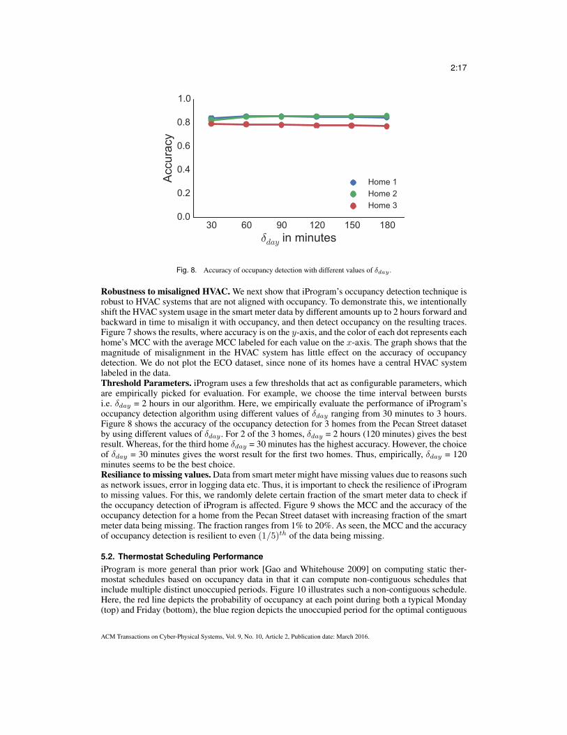
Fig. 8. Accuracy of occupancy detection with different values of �day .

Robustness to misaligned HVAC. We next show that iProgram’s occupancy detection technique isrobust to HVAC systems that are not aligned with occupancy. To demonstrate this, we intentionallyshift the HVAC system usage in the smart meter data by different amounts up to 2 hours forward andbackward in time to misalign it with occupancy, and then detect occupancy on the resulting traces.Figure 7 shows the results, where accuracy is on the y-axis, and the color of each dot represents eachhome’s MCC with the average MCC labeled for each value on the x-axis. The graph shows that themagnitude of misalignment in the HVAC system has little effect on the accuracy of occupancydetection. We do not plot the ECO dataset, since none of its homes have a central HVAC systemlabeled in the data.Threshold Parameters. iProgram uses a few thresholds that act as configurable parameters, whichare empirically picked for evaluation. For example, we choose the time interval between burstsi.e. �

day

= 2 hours in our algorithm. Here, we empirically evaluate the performance of iProgram’soccupancy detection algorithm using different values of �

day

ranging from 30 minutes to 3 hours.Figure 8 shows the accuracy of the occupancy detection for 3 homes from the Pecan Street datasetby using different values of �

day

. For 2 of the 3 homes, �day

= 2 hours (120 minutes) gives the bestresult. Whereas, for the third home �

day

= 30 minutes has the highest accuracy. However, the choiceof �

day

= 30 minutes gives the worst result for the first two homes. Thus, empirically, �day

= 120minutes seems to be the best choice.Resiliance to missing values. Data from smart meter might have missing values due to reasons suchas network issues, error in logging data etc. Thus, it is important to check the resilience of iProgramto missing values. For this, we randomly delete certain fraction of the smart meter data to check ifthe occupancy detection of iProgram is affected. Figure 9 shows the MCC and the accuracy of theoccupancy detection for a home from the Pecan Street dataset with increasing fraction of the smartmeter data being missing. The fraction ranges from 1% to 20%. As seen, the MCC and the accuracyof occupancy detection is resilient to even (1/5)th of the data being missing.

5.2. Thermostat Scheduling PerformanceiProgram is more general than prior work [Gao and Whitehouse 2009] on computing static ther-mostat schedules based on occupancy data in that it can compute non-contiguous schedules thatinclude multiple distinct unoccupied periods. Figure 10 illustrates such a non-contiguous schedule.Here, the red line depicts the probability of occupancy at each point during both a typical Monday(top) and Friday (bottom), the blue region depicts the unoccupied period for the optimal contiguous


2:18

Fig. 9. MCC and Accuracy of occupancy detection for a home with increasing amnoutn of missing values.


0.0

0.2

0.4

0.6

0.8

1.0

1.2

Occ

upan

cyP

roba

bilit

y

contiguous non-contiguous


0.0

0.2

0.4

0.6

0.8

1.0

1.2

Occ

upan

cyP

roba

bilit

y

Fig. 10. Illustration of the benefits of a non-contiguous thermostat schedule with multiple unoccupied periods.

schedule, which is restricted to a single unoccupied period, and the green region depicts the unoc-cupied periods of the optimal non-contiguous schedule. On both days, there is a slight increase inthe occupancy probability near the middle of the day at lunchtime, presumably resulting from theoccupants coming home for lunch. Our optimal non-contiguous schedule recognizes this and turnson the HVAC system (indicated by the lack of the green regions when the probability rises), whilethe contiguous schedule keeps the HVAC system off (indicated by the remaining blue region whenthe probability rises). The optimal non-contiguous schedule reduces the overall miss time of theresulting schedule by 20 minutes across both days compared to the optimal contiguous schedule.Robustness to misaligned HVAC. Figure 11 shows the optimal mismatch time for homes in thePecan Street dataset, where we shift the HVAC system usage from 0 to 2 hours to misalign it withoccupancy. Our results show that iProgram’s schedules are robust to such misalignments, as themismatch time across homes does not vary significantly with the shift in HVAC usage. The graphalso shows that the average optimal mismatch time for the Pecan Street data set is near 60 minutes,although the average is affected by a few homes with very large mismatch times; 75% of the homeshave a mismatch time below 60 minutes and 50% of them have a mismatch time <30 minutes.Convergence results. For iProgram to be adopted by residential home owners, it is essential toshow that near-optimal static schedules are generated with a minimal amount of data. Here, we


2:19

0 20 40 60 80 100Home ID

0

100

200

300

400

500

600

Mis

mat

ch(m

inut

es)

Misalignment shift (hour)-2.0-1.5-1.0

-0.50.00.5

1.01.52.0

Fig. 11. The mismatch time for homes in the Pecan Street dataset with different shifts in the HVAC system usage.

1 2 3 4 5 6 7 8 9Week number

0

10

20

30

40

50

60

MT

(min

utes

)

1 2 3 4 5 6 7 8 9Week number

0

50

100

150

200

250

300

WT

(min

utes

)

(a) Miss time (b) Waste time

Fig. 12. Convergence of custom schedules for homes from the Pecan street dataset.

show empirical results that demonstrate the effectiveness of iProgram to quickly converge to a fixedstatic schedule with limited smart meter energy consumption data. Figure 12 shows the miss timeand waste time for homes in the Pecan Street dataset in the form of boxplots over increasing numberof weeks of smart meter data available. The miss time target used for this experiment is 60 minutes.With just one week of available data, the average miss time for all homes is around 15 minutes.However, this reduces to just over 12 minutes when data for two weeks is available. Similarly, withone week’s data, the average waste time is around 100 minutes. However, this reduces to 60-75minutes with two or more weeks of data available.

5.3. Schedule Baseline ComparisonIn this section, we evaluate the schedules generated by iProgram. For this experiment, we restrictedour analysis to weekdays only. Further, we also extend our analysis to a couple of schedule gen-


2:20

Fig. 13. Comparison among the schedule generation techniques such as iProgram, Base-ct, and Base-mt. All these arecompared with the default baseline schedule.

eration algorithms from [Gao and Whitehouse 2009] i.e. Base-ct and Base-mt. Base-ct minimizesmiss time while maintaining a certain unconditioned time. Whereas, Base-mt maximizes the uncon-ditioned time while maintaining the same miss time as the baseline schedule. Thus, the parametersfor Base-ct and Base-mt are unconditioned time and miss time respectively.

In this evaluation, we selected parameters such that we have a fair comparison among the differentscheduling algorithms. iProgram, similar to Base-mt, has miss time as the input parameter. Wechose this parameter to be equal to 60 minutes for both these scheduling algorithms. Further, Base-ct has unconditioned time as the input parameter. We chose this to be 10 hours, i.e., same as that forthe baseline schedule (8:00 AM to 6:00 PM).

All the 3 algorithms are compared to the baseline schedule, i.e., the default setting on an Ener-gyStar compliant thermostat (8:00 AM to 6:00 PM). Figure 13 shows the Cumulative DistributionFunction (CDF) of the difference between the mismatch time of the baseline schedule with the 3algorithms for all the 100 homes from the Pecan Street dataset. Thus, a negative value indicates animprovement in performance compared to the baseline. Further, the black horizontal line highlightsthe performance of a median home.

As indicated by the narrow spread of the graph, Base-ct’s performance is very close to the base-line. The median value of the difference in mismatch time is 1.17 minute, i.e., slightly worse thanthe baseline. Base-mt algorithm has a greater spread in the difference in mismatch times than Base-ct. Further, this variation in performance among homes is much higher for iProgram. However,the median value difference in mismatch time is -36.5 minutes for Base-mt. Thus, Base-mt outper-forms the baseline and Base-ct. Both Base-mt and iProgram outperform the baseline for 61 homes.Further, the median value of the difference in mismatch time with the baseline is -43.0 minutes, i.e.,better than all other algorithms.

Looking closely at the schedules for these homes, we observe that the large positive value ofthe difference in mismatch time for multiple homes is due to occupancy with low human activity.This results in iProgram incorrectly classifying a period as unoccupied when it is occupied. Thesehomes can leverage iProgram’s feedback module described in subsection 3.3 discussing schedulingextensions to correct the misclassification.


2:21

Wee

k1 Mismatchimprovement = 0 minutes

Static schedule Adaptive schedule

Wee


Wee


12 AM 4 AM 8 AM 12 PM 4 PM 8 PM 12 AMUnconditioned Time

Wee


Fig. 14. iProgram’s schedule adapts as occupancy changes.

5.4. Dynamic Schedule GenerationFigure 14 illustrates iProgram’s ability to adapt to changes in a the pattern of occupancy. In this case,iProgram computes a schedule using one month of data from a representative home. We then swapevery Wednesday and Sunday for the next month to simulate a change in working hours. The graphthen shows two schedules: static, where the schedule is generated using the first month’s occupancy,and adaptive, where schedules are generated using a moving window of 1 month. In the first week,both static and adaptive approaches derive the same schedule as they are using data for the sametime period. As shown, iProgram adapts quickly to the changed schedule with new data availableevery week.Frequency of deriving schedules. In the design section, we discussed the use of Manhattan dis-tance to compares changes in occupancy patterns to flag if there is a need to re-run the schedulegeneration algorithm. To demonstrate how frequently we need to re-derive schedules, we use thePecan Street dataset containing 100 homes. We initially use 8 weeks of smart meter data to inferoccupancy patterns and to generate custom schedules. Then, we apply the schedule derived on thenext week. If the occupancy pattern change measured by Manhattan distance is more than a certainthreshold (mismatch time), the schedule generation algorithm is called to derive newer schedulesaccounting for newer data available.

Figure 15 shows the frequency distribution of the number of homes out of 100 that requiredre-derivation of custom schedules each week after the first 8 weeks. The mismatch time thresholdfor this experiment needed to leverage Manhattan distance measure is set to 2 hours. As observed,no more than 13 homes change their occupancy pattern significantly to merit re-derivation for anyweek. Further, for most weeks, less than 10 homes require fresh schedules. Thus, we find thatmajority of homes do not change their schedule significantly.

Figure 16 shows the difference between the miss times recorded for periodically re-derivingschedules and the Manhattan distance-based approach represented as boxplots. Again, the completePecan Street dataset containing 100 homes was used for this experiment. As seen, for most homesthe difference is negligible — suggesting our Manhattan distance-based approach has no significantdegradation when compared to the periodically re-deriving schedules. However, the worst averagedifference in miss times of around 4 minutes is observed for week 26. For week 26, 93 of the 100homes have the difference in miss time no worse than 30 minutes.


2:22

8 9 10 11 12 13 14 15 16 17 18 19 20 21 22 23 24 25 26Week Number

0

2

4

6

8

10

12

14

Freq

uenc

ydi

stribu

tion

ofho

mes

Fig. 15. Frequency distribution of number of homes in Pecan Street dataset with re-derivation of custom schedules trig-gered by Manhattan distance based measure.

9 10 11 12 13 14 15 16 17 18 19 20 21 22 23 24 25 26Week Number

�30

�20

�10

0

10

20

30

�M

T(P

erio

dic

-M

anha

ttan

)

Fig. 16. Difference in miss times for the different weeks for all homes in Pecan Street dataset.

5.5. Energy SavingsFigure 17 shows the estimated average daily energy savings each home in the Pecan Street datasetcould achieve over 6 months using iProgram with different target miss times. Each point on thex-axis represents the estimated energy savings for a home, where we order homes by their energysavings when using a 1-day schedule. Here, we estimate the energy savings assuming the HVACsystem uses iProgram’s schedule; we then count any energy consumed by the HVAC system duringan off period in the schedule towards our savings. Of course, the HVAC system may occasionallyturn on during unoccupied periods to maintain the setback. In this case, we assume the setback issufficiently deep that occupants are not away long enough for the temperature to reach it.


2:23

Fig. 17. Estimated energy savings for different target miss times for each home in the Pecan Street dataset.

The graph shows that, as expected, a 7-day schedule achieves slightly more energy savings than a5-2-day schedule, which in turn achieves slightly more savings than a 1-day schedule. However, thesavings relative to a 1-day schedule, while significant in some homes, are not significant on average.Also as expected, the greater the acceptable target miss time (and the lower the tolerable comfortlevel), the more energy savings the homes achieve. The maximum energy savings (with a miss timeof 60 minutes) is near 2.5kWh per day, which is over 10% of a typical U.S. home’s average dailyenergy usage. Overall, the average daily energy savings is in the range of 0.25 kWh (for a 15 minutemiss time) to 1.0kWh (for a 60 minute miss time), which represents a 1-5% energy reduction in anaverage U.S. home. However, the strength of our approach does not lie in achieving large energysavings in a small number of homes, as with smart thermostats, but rather in being immediatelyapplicable to saving energy across a large number of homes.

We also compare iProgram’s schedule to a default 8am-6pm thermostat schedule. We find that itreduces the mismatch time by a median value of 44.28 minutes (out of the 100 homes) for a weekdayschedule, with a median deviation of 30.76 minutes off the optimal schedule (assuming perfectoccupancy). In this case, iProgram would yield a daily energy savings of 0.42kWh on averageacross the 100 homes. Note that this estimated energy savings is conservative, since most PecanStreet homes are already highly efficient, and have little room for improvement. The Pecan Streetparticipants have volunteered to have their homes instrumented by Pecan Street and are highly awareof their energy usage. Thus, we expect the energy savings possible in a typical U.S. home is likelyto be much higher.


2:24

15 30 45 60Miss Time target (minutes)

0

50

100

150

200

250

300

350

Unc

ondi

tion

edT

ime

(min

utes

)

House

Zone1

Zone2

Fig. 18. Unconditioned times for the overall home along with the two zones for different miss time targets.

5.6. Zonal schedulesAs discussed earlier, quite a few homes have different zones with a dedicated HVAC unit control-ling them separately. This provides an increased potential for iProgram to learn occupancy patternsfor these zones independently, provided submetered electricity data for each zone is available. Asresidents occupy different parts of the house during the different times of the day, there is significantpotential to improve/reduce the energy consumption of homes. Figure 18 shows the increase in theunconditioned time of the HVAC system in a home from Smart* dataset with zone level subme-tered energy data available. Zone1 consists of Living room, dining room, and guest rooms, whereasZone2 consists of Kitchen and the different bedrooms. The figure shows the unconditioned time fordifferent miss time targets. As seen, the unconditioned time for home and the Zone2 is exactly thesame i.e. the Zone2 is always occupied when the resident is at home. However, Zone1 has a largerunconditioned time for different miss time targets. The magnitude of unconditioned time comparedto the Zone2 and home is significant — in the range of 40% to 70%.

5.7. Case StudyAs discussed in the early sections of the paper, installing occupancy sensors en-masse may not befeasible. However, with the proliferation of smartphones, indirect sensing of occupancy can be usedto improve the accuracy of the schedules generated using iProgram. We present a case-study whereresidents phone connecting and disconnecting to the home WiFi network is used to infer occupancy.One can use an IFTTT recipe to collect this information similar to [IFTTT Recipe 2015]. The dataused is from the Home2 of the Smart* dataset.

Figure 19 compares the miss times for inferred occupancy from smart meter data and sensedoccupancy from the smart phone. Miss times are recorded for the different miss time targets. Asshown, there is an improvement in the miss times in the range of 20 to 40 minutes for different misstime targets. Thus, additional information about user occupancy can be used to improve customschedules.

5.8. User StudyTo validate our algorithm in a real world setting, we conducted a user study, which asked participantsto rate the schedules generated by iProgram for their respective homes. The objective of the studywas to i) get user feedback on iProgram’s schedules, ii) better understand user interactions with


2:25

0 50 100 150 200Miss Time target (minutes)

0

50

100

150

200

250

Miss

Tim

e(m

inut

es)

Sensed Occupancy

Inferred Occupancy

Fig. 19. Recorded miss times for sensed and inferred occupancy for different miss time targets.

their thermostats, and iii) validate scheduling anomalies identified by iProgram. We worked witha local utility company in the northeast U.S. to solicit 8 anonymous users for the study. Each userconsented to analysis of their smart meter data, which was anonymized to preserve the privacy ofthe participants. In this case, the data for each home covered a 3 month period with average powerdata recorded every 5 minutes. We used iProgram to derive a 7-day schedule, and then presenteda customized questionnaire to each participant that asked them to rate their schedule on a scale of1 (does not match my occupancy pattern) to 5 (perfectly matches). In addition, the questionnaireincluded questions about the type and usage of the home’s thermostat, and the weekly work patternsof the home’s occupants. We also included customized questions to corroborate any anomalies inthe schedule derived by iProgram. Such anomalies included long periods of low electricity usageover multiple days, a repeating unoccupied period on one specific day of the week, etc.

Based on the results, we discovered each participant had a programmable thermostat in theirhome, but all the homes manually adjusted the thermostat without programming it. Most the par-ticipants work patterns followed a 5-2-day schedule, although one home included a retired couplewith a much higher rate of occupancy. iProgram was also able to correctly identify a majority ofthe scheduling anomalies discovered during the analysis. Figure 20 shows the participants’ ratingsof iProgram’s schedule for different days of the week. The figure shows that 73% of the schedulesand derived occupancy patterns got ratings of 3 or higher. In addition, participant P4, which was theretired couple, gave a poor rating for weekdays. In this case, the occupants were frequently home onweekdays but did not consume much electricity, so iProgram identified these periods as unoccupiedwhen generating its schedule.5 Finally, 5 of the participants had an average rating above 3, and 3 ofthe participants had an average rating above 4 across all days.

6. DISCUSSION6.1. Temperature SettingAs discussed earlier, iProgram makes use of existing programmable thermostats and utility smartmeters to infer schedules. The schedules can be programmed into the thermostat to toggle betweensetpoint and setback temperatures. Typical setpoint temperature suggested by American Society ofHeating, Refrigerating and Air-Conditioning Engineers is 68�F. However, personal preferences of

5We have refined our approach to to better capture burstiness and to interpolate across detected bursty periods.


2:26

Monday Tuesday Wednesday Thursday Friday Saturday SundayDay

P8

P7

P6

P5

P4

P3

P2

P1

Parti

cipa

nt

2

1

3

1

3

4

2

4

3

2

2

1

1

4

5

4

3

3

2

1

3

4

5

4

3

3

5

1

1

3

4

4

3

4

5

1

2

5

5

4

3

5

4

4

4

5

4

4

3

5

4

4

4

5

4

4

1.6

2.4

3.2

4.0

4.8

Fig. 20. User ratings of iProgram’s thermostat schedules for different days of the week. Over 73% of the daily scheduleshave good ratings of 3 or higher.

the users and the building materials of the home may dictate a different setpoint for ensuring humancomfort. Several people refrain from using the setback feature of the thermostat due to discomfortexperienced when in contact with objects in the house. Thus, human discomfort is dependent on notjust the ambient air temperature but also on the radiant temperature of the surrounding environment.Building Energy Standards [passivhaus 2017] have proposed a maximum difference of 6�F betweenthe coldest surface in the house and the ambient air temperature. To ensure occupant comfort, HVACsystems may be configured to have a higher setback temperature than the default settings (typicallyset at 60�F). Moreover, to ensure user comfort, we can set the home to be sufficiently pre-heated inwinter and pre-cooled in summer before the users arrival. Although the time to reach the setpointdepends on the outside temperatures and the duration of unconditioned time, we can fix this toaround be 15-20 minutes.

6.2. Designing Energy Efficiency Nudges[Lutzenhiser et al. 2004] presented an interesting case-study where the homeowners in Californiavoluntarily reduced their AC usage and showed flexibility in energy demands, for reasons other thanpersonal energy bill. Through conservation campaigns, the homeowners learned how their actionscan reduce a possible energy crisis. Due to these actions, state-wide energy usage reduction wasexperienced during a heat wave. Similar conservation campaigns might be designed around the useof iProgram when adopted en masse. For example, homeowners might be motivated to set aggressiveschedules (i.e. with higher miss time) or lower setpoint and setback temperatures during winters.These homeowners can be presented with their contribution in the form of energy units reducedtowards the overall energy efficiency goal at city/county level.

7. CONCLUSIONIn this paper, we present iProgram, a system for inferring smart schedules for programmable ther-mostats from smart meter data. iProgram cannot directly apply prior work on occupancy detectionfrom smart meter data due to its application context, which does not provide access to training dataand has a particular emphasis on inefficient homes with misaligned thermostats. Thus, we designa more targeted occupancy detection approach, which leverages time-series component analysis toisolate the burstiness of interactive loads. In addition, we show how to translate inferred patternsof occupancy into an optimal static thermostat schedule. We implement iProgram as a web service,


2:27

and evaluate it across data from over 100 homes, as well as conduct a user study to verify its efficacyin real homes.

Our evaluation showed that iProgram reduces the mismatch time between the occupancy patternand the thermostat schedule by 44.28 minutes when compared to a default 8am-6pm schedule, and isonly 30.76 minutes on average off a schedule that precisely tracks occupancy. We also showed thatthe schedules generated from iProgram converge to optimal schedules within a couple of weeks formost homes. We also discussed that homeowners having multiple HVAC zones can utilize iProgramand can significantly increase unconditioned times of less occupied parts of their homes. As partof future work, we plan to work with a local utility to include iProgram’s suggested thermostatschedules in real energy bills and as part of energy audits.

8. ACKNOWLEDGEMENTSThis research was supported by NSF grants IIP-1534080, CNS-1405826, CNS-1253063, and theMassachusetts Department of Energy Resources.

APPENDIXELECTRONIC APPENDIXThe electronic appendix for this article can be accessed in the ACM Digital Library.

ACKNOWLEDGMENTS

REFERENCES

Y. Agarwal, B. Balaji, S. Dutta, R.K. Gupta, and T. Weng. 2011. Duty-cycling Buildings Aggres-sively: The Next Frontier in HVAC Control. In IPSN.

S. Barker, A. Mishra, D. Irwin, E. Cecchet, P. Shenoy, and J. Albrecht. 2012. Smart*: An OpenData Set and Tools for Enabling Research in Sustainable Homes. In SustKDD.

C. Beckel, W. Kleiminger, R. Cicchetti, T. Staake, and S. Santini. 2014. The ECO Data Set and thePerformance of Non-Intrusive Load Monitoring Algorithms. In BuildSys.

D. Chen, Sean Barker, A. Subbaswamy, D. Irwin, and P. Shenoy. 2013. Non-Intrusive OccupancyMonitoring using Smart Meters. In BuildSys.

D. Chen, D. Irwin, P. Shenoy, and J. Albrecht. 2014. Combined Heat and Privacy: PreventingOccupancy Detection from Smart Meters. In PerCom.

S. Clark, B. Ransford, and K. Fu. 2012. Potentia est Scientia: Security and Privacy Implications ofEnergy-Proportional Computing. In HotSec.

ecobee 2015. Ecobee. http://ecobee.com. (January 2015).eia 2009. U.S. Energy Information Administration, Frequently Asked Questions, Residential Energy

Consumption Survey (RECS). http://www.eia.gov/consumption/residential/data/2009/. (2009).eia 2014. U.S. Energy Information Administration, Most Homes have Central Thermostats on Heat-

ing and Cooling Equipment. http://www.eia.gov/todayinenergy/detail.cfm?id=14771. (January28th 2014).

V. Erickson, M. Carreira-Perpinan, and A. Cerpa. 2011. OBSERVE: Occupancy-based System forEfficient Reduction of HVAC Energy. In IPSN.

V. Erickson and A. Cerpa. 2010. Occupancy Based Demand Response HVAC Control Strategy. InBuildSys.

K. Fehrenbacher. 2012. 75% of U.S. Electric Meters will be Smart by 2016. In Gigaom Research.G. Gao and K. Whitehouse. 2009. The Self-programming Thermostat: Optimizing Setback Sched-

ules based on Home Occupancy Patterns. In BuildSys.IFTTT Recipe 2015. Home Occupancy Detector. https://ifttt.com/recipes/

276032-home-occupancy-detector. (January 2015).Srinivasan Iyengar, Stephen Lee, David Irwin, and Prashant Shenoy. 2016. Analyzing Energy Us-

age on a City-scale using Utility Smart Meters. In Proceedings of the 3rd ACM International


2:28

Conference on Systems for Energy-Efficient Built Environments. ACM, 51–60.J. St. John. 2014. 50 Million U.S. Smart Meters and Counting. In GreenTech Grid.J. Kelso (Ed.). 2012. 2011 Buildings Energy Data Book. Department of Energy.W. Kleiminger, C. Beckel, T. Staake, and S. Santini. 2013. Occupancy Detection from Electricity

Consumption Data. In BuildSys.J. Kolter and M. Johnson. 2011. REDD: A Public Data Set for Energy Disaggregation Research. In

SustKDD.J. Lu, T. Sookoor, V. Srinivasan, G. Gao, B. Holben, J. Stankovic, E. Field, and K. Whitehouse.

2010. The Smart Thermostat: Using Occupancy Sensors to Save Energy in Homes. In SenSys.Loren Lutzenhiser, Huafen Hu, Mithra Moezzi, Anthony Levenda, and James Woods. 2012.

Lifestyles, Buildings and Technologies: What Matters Most. In ACEEE Summer Study on En-ergy Efficiency in Buildings, Vol. 2. 256–270.

Loren Lutzenhiser, Rick Kunkle, James Woods, Susan Lutzenhiser, and Sylvia Bender. 2004. Last-ing impressions: conservation and the 2001 California energy crisis. In Proceedings, AmericanCouncil for an Energy Efficient Economy.

lyric 2015. Honeywell Lyric. http://lyric.honeywell.com. (January 2015).nest 2015. Nest. http://nest.com. (January 2015).M. Nevius and S. Pigg. 2000. Programmable Thermostats that Go Berserk? Taking a Social Per-

spective on Space Heating in Wisconsin. ACEEE Summer Study on Energy Efficiency in Buildings8 (December 2000).

passivhaus 2017. Passivhaus. http://www.passiv.de/. (June 2017).pecan 2015. Pecan Street. http://www.pecanstreet.org/. (January 2015).T. Peffer, M. Pritoni, A. Meier, C. Aragon, and D. Perry. 2011. How People use Thermostats in

Homes: A Review. Building and Environment 46, 12 (December 2011).J. Scott, A.J. Brush, J. Krumm, B. Meyers, M. Hazas, S. Hodges, and N. Villar. 2011. PreHeat:

Controlling Home Heating Using Occupancy Prediction. In Ubicomp.J. Seabold and J. Perktold. 2010. Statsmodels: Econometric and Statistical Modeling with Python.

In Scipy.S. Shakkottai and N. Brownlee. 2005. A Study of Burstiness in TCP Flows. In PAM.Elizabeth Shove, Heather Chappells, Loren Lutzenhiser, and Bruce Hackett. 2008. Comfort in a

lower carbon society. (2008).

Received February 2007; revised March 2009; accepted June 2009


2 inferring smart schedules for dumb thermostatslass.cs.umass.edu/papers/pdf/iprogram_tcps.pdf · 2...

Documents