FRE

EC

OP

Y2

Introduction

When you want to become a sculptor1 you have to learn some basic techniques:where to get the right stones, how to move them, how to handle the chisel, how toerect scaffolding, . . . . Knowing these techniques will not make you a famous artist,but even if you have a really exceptional talent, it will be very difficult to developinto a successful artist without knowing them. It is not necessary to master all of thebasic techniques before sculpting the first piece. But you always have to be willingto go back to improve your basic techniques.

This introductory chapter plays a similar role in this book.We introduce basicconcepts that make it simpler to discuss and analyze algorithms in the subsequentchapters. There is no need for you to read this chapter from beginning to end beforeyou proceed to later chapters. On first reading, we recommendthat you should readcarefully to the end of Sect. 2.3 and skim through the remaining sections. We begin inSect. 2.1 by introducing some notation and terminology thatallow us to argue aboutthe complexity of algorithms in a concise way. We then introduce a simple machinemodel in Sect. 2.2 that allows us to abstract from the highly variable complicationsintroduced by real hardware. The model is concrete enough tohave predictive valueand abstract enough to allow elegant arguments. Section 2.3then introduces a high-level pseudocode notation for algorithms that is much more convenient for express-ing algorithms than the machine code of our abstract machine. Pseudocode is alsomore convenient than actual programming languages, since we can use high-levelconcepts borrowed from mathematics without having to worryabout exactly howthey can be compiled to run on actual hardware. We frequentlyannotate programsto make algorithms more readable and easier to prove correct. This is the subjectof Sect. 2.4. Section 2.5 gives the first comprehensive example: binary search in asorted array. In Sect. 2.6, we introduce mathematical techniques for analyzing thecomplexity of programs, in particular, for analyzing nested loops and recursive pro-

1 The above illustration of Stonehenge is from [156].

FRE

EC

OP

Y20 2 Introduction

cedure calls. Additional analysis techniques are needed for average-case analysis;these are covered in Sect. 2.7. Randomized algorithms, discussed in Sect. 2.8, usecoin tosses in their execution. Section 2.9 is devoted to graphs, a concept that willplay an important role throughout the book. In Sect. 2.10, wediscuss the question ofwhen an algorithm should be called efficient, and introduce the complexity classesP andNP. Finally, as in every chapter of this book, there are sections containing im-plementation notes (Sect. 2.11) and historical notes and further findings (Sect. 2.12).

2.1 Asymptotic Notation

The main purpose of algorithm analysis is to give performance guarantees, for ex-ample bounds on running time, that are at the same time accurate, concise, general,and easy to understand. It is difficult to meet all these criteria simultaneously. Forexample, the most accurate way to characterize the running timeT of an algorithm isto viewT as a mapping from the setI of all inputs to the set of nonnegative numbersR+. For any problem instancei, T(i) is the running time oni. This level of detail isso overwhelming that we could not possibly derive a theory about it. A useful theoryneeds a more global view of the performance of an algorithm.

We group the set of all inputs into classes of “similar” inputs and summarize theperformance on all instances in the same class into a single number. The most usefulgrouping is bysize. Usually, there is a natural way to assign a size to each probleminstance. The size of an integer is the number of digits in itsrepresentation, and thesize of a set is the number of elements in the set. The size of aninstance is alwaysa natural number. Sometimes we use more than one parameter tomeasure the sizeof an instance; for example, it is customary to measure the size of a graph by itsnumber of nodes and its number of edges. We ignore this complication for now. Weuse size(i) to denote the size of instancei, andIn to denote the instances of sizenfor n∈N. For the inputs of sizen, we are interested in the maximum, minimum, andaverage execution times:2

worst case: T(n) = maxT(i) : i ∈ Inbest case: T(n) = minT(i) : i ∈ Inaverage case: T(n) =

1|In| ∑

i∈In

T(i) .

We are interested most in the worst-case execution time, since it gives us thestrongest performance guarantee. A comparison of the best case and the worst casetells us how much the execution time varies for different inputs in the same class. Ifthe discrepancy is big, the average case may give more insight into the true perfor-mance of the algorithm. Section 2.7 gives an example.

We shall perform one more step of data reduction: we shall concentrate ongrowthrate or asymptotic analysis. Functionsf (n) andg(n) have thesame growth rateif

2 We shall make sure thatT(i) : i ∈ In always has a proper minimum and maximum, andthat In is finite when we consider averages.

FRE

EC

OP

Y2.1 Asymptotic Notation 21

there are positive constantsc andd such thatc≤ f (n)/g(n) ≤ d for all sufficientlylarge n, and f (n) grows fasterthan g(n) if, for all positive constantsc, we havef (n) ≥ c · g(n) for all sufficiently largen. For example, the functionsn2, n2 + 7n,5n2− 7n, andn2/10+ 106n all have the same growth rate. Also, they grow fasterthann3/2, which in turn grows faster thannlogn. The growth rate talks about thebehavior for largen. The word “asymptotic” in “asymptotic analysis” also stressesthe fact that we are interested in the behavior for largen.

Why are we interested only in growth rates and the behavior for largen? We areinterested in the behavior for largen because the whole purpose of designing efficientalgorithms is to be able to solve large instances. For largen, an algorithm whoserunning time has a smaller growth rate than the running time of another algorithmwill be superior. Also, our machine model is an abstraction of real machines andhence can predict actual running times only up to a constant factor, and this suggeststhat we should not distinguish between algorithms whose running times have thesame growth rate. A pleasing side effect of concentrating ongrowth rate is that wecan characterize the running times of algorithms by simple functions. However, inthe sections on implementation, we shall frequently take a closer look and go beyondasymptotic analysis. Also, when using one of the algorithmsdescribed in this book,you should always ask yourself whether the asymptotic view is justified.

The following definitions allow us to argue precisely aboutasymptotic behavior.Let f (n) andg(n) denote functions that map nonnegative integers to nonnegative realnumbers:

O( f (n)) = g(n) : ∃c > 0 :∃n0 ∈ N+ : ∀n≥ n0 : g(n) ≤ c · f (n) ,

Ω( f (n)) = g(n) : ∃c > 0 :∃n0 ∈ N+ : ∀n≥ n0 : g(n) ≥ c · f (n) ,

Θ( f (n)) = O( f (n))∩Ω( f (n)) ,

o( f (n)) = g(n) : ∀c > 0 :∃n0 ∈ N+ : ∀n≥ n0 : g(n) ≤ c · f (n) ,

ω( f (n)) = g(n) : ∀c > 0 :∃n0 ∈ N+ : ∀n≥ n0 : g(n) ≥ c · f (n) .

The left-hand sides should be read as “big O off ”, “big omega of f ”, “theta of f ”,“little o of f ”, and “little omega off ”, respectively.

Let us see some examples. O(

n2)

is the set of all functions that grow at mostquadratically, o

(

n2)

is the set of functions that grow less than quadratically, ando(1) is the set of functions that go to zero asn goes to infinity. Here “1” standsfor the functionn 7→ 1, which is one everywhere, and hencef ∈ o(1) if f (n) ≤c · 1 for any positivec and sufficiently largen, i.e., f (n) goes to zero asn goes toinfinity. Generally, O( f (n)) is the set of all functions that “grow no faster than”f (n).Similarly, Ω( f (n)) is the set of all functions that “grow at least as fast as”f (n). Forexample, the Karatsuba algorithm for integer multiplication has a worst-case runningtime in O

(

n1.58)

, whereas the school algorithm has a worst-case running timeinΩ(

n2)

, so that we can say that the Karatsuba algorithm is asymptotically faster thanthe school algorithm. The “little o” notation o( f (n)) denotes the set of all functionsthat “grow strictly more slowly than”f (n). Its twin ω( f (n)) is rarely used, and isonly shown for completeness.

FRE

EC

OP

Y22 2 Introduction

The growth rate of most algorithms discussed in this book is either a polynomialor a logarithmic function, or the product of a polynomial anda logarithmic func-tion. We use polynomials to introduce our readers to some basic manipulations ofasymptotic notation.

Lemma 2.1.Let p(n) = ∑ki=0aini denote any polynomial and assume ak > 0. Then

p(n) ∈ Θ(

nk)

.

Proof. It suffices to show thatp(n)∈ O(

nk)

andp(n)∈ Ω(

nk)

. First observe that forn > 0,

p(n) ≤k

∑i=0

|ai |ni ≤ nkk

∑i=0

|ai | ,

and hencep(n) ≤ (∑ki=0 |ai |)nk for all positiven. Thusp(n) ∈ O

(

nk)

.Let A = ∑k−1

i=0 |ai |. For positiven we have

p(n) ≥ aknk−Ank−1 =

ak

2nk +nk−1

(ak

2n−A

)

and hencep(n) ≥ (ak/2)nk for n > 2A/ak. We choosec = ak/2 andn0 = 2A/ak inthe definition ofΩ

(

nk)

, and obtainp(n) ∈ Ω(

nk)

. ⊓⊔

Exercise 2.1.Right or wrong? (a)n2+106n∈O(

n2)

, (b)nlogn∈O(n), (c)nlogn∈Ω(n), (d) logn∈ o(n).

Asymptotic notation is used a lot in algorithm analysis, andit is convenient tostretch mathematical notation a little in order to allow sets of functions (such asO(

n2)

) to be treated similarly to ordinary functions. In particular, we shall alwayswrite h = O( f ) instead ofh∈ O( f ), and O(h) = O( f ) instead of O(h) ⊆ O( f ). Forexample,

3n2 +7n= O(

n2)= O(

n3) .

Be warned that sequences of equalities involving O-notation should only be readfrom left to right.

If h is a function,F andG are sets of functions, and is an operator such as+, ·, or /, thenF G is a shorthand for f g : f ∈ F,g∈ G, andhF stands forh F. So f (n)+ o( f (n)) denotes the set of all functionsf (n)+ g(n) whereg(n)grows strictly more slowly thanf (n), i.e., the ratio( f (n)+ g(n))/ f (n) goes to oneasn goes to infinity. Equivalently, we can write(1+o(1)) f (n). We use this notationwhenever we care about the constant in the leading term but want to ignorelower-order terms.

Lemma 2.2.The following rules hold forO-notation:

c f(n) = Θ( f (n)) for any positive constant,

f (n)+g(n) = Ω( f (n)) ,

f (n)+g(n) = O( f (n)) if g(n) = O( f (n)) ,

O( f (n)) ·O(g(n)) = O( f (n) ·g(n)) .

FRE

EC

OP

Y2.2 The Machine Model 23

Exercise 2.2.Prove Lemma 2.2.

Exercise 2.3.Sharpen Lemma 2.1 and show thatp(n) = aknk +o(

nk)

.

Exercise 2.4.Prove thatnk = o(cn) for any integerk and anyc> 1. How doesnlog logn

compare withnk andcn?

2.2 The Machine Model

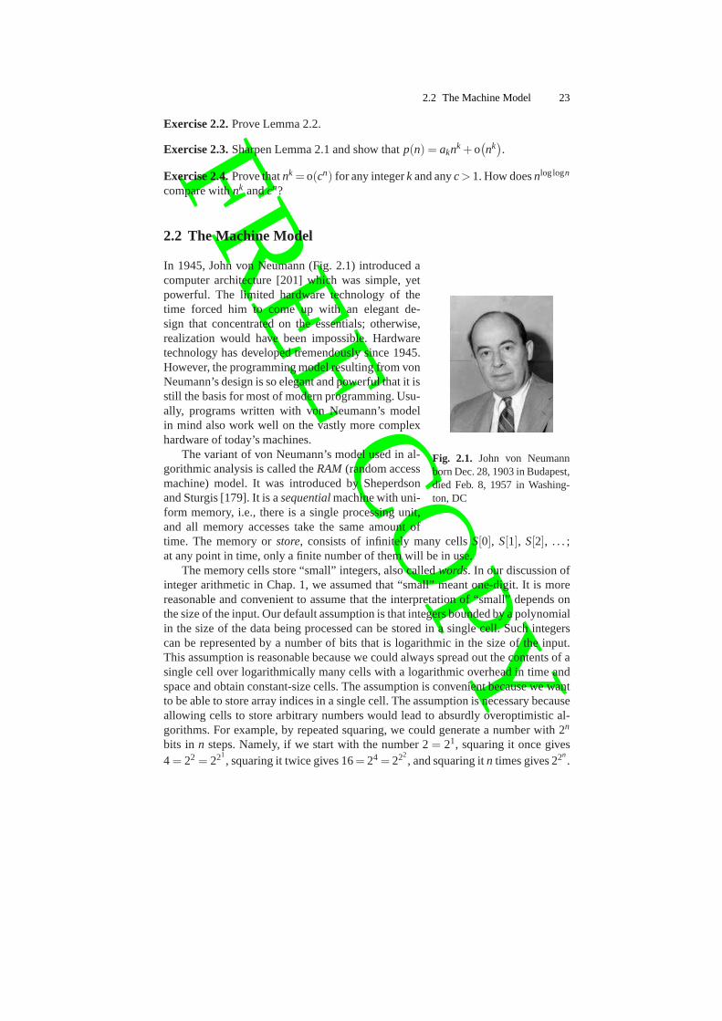
Fig. 2.1. John von Neumannborn Dec. 28, 1903 in Budapest,died Feb. 8, 1957 in Washing-ton, DC

In 1945, John von Neumann (Fig. 2.1) introduced acomputer architecture [201] which was simple, yetpowerful. The limited hardware technology of thetime forced him to come up with an elegant de-sign that concentrated on the essentials; otherwise,realization would have been impossible. Hardwaretechnology has developed tremendously since 1945.However, the programming model resulting from vonNeumann’s design is so elegant and powerful that it isstill the basis for most of modern programming. Usu-ally, programs written with von Neumann’s modelin mind also work well on the vastly more complexhardware of today’s machines.

The variant of von Neumann’s model used in al-gorithmic analysis is called theRAM (random accessmachine) model. It was introduced by Sheperdsonand Sturgis [179]. It is asequentialmachine with uni-form memory, i.e., there is a single processing unit,and all memory accesses take the same amount oftime. The memory orstore, consists of infinitely many cellsS[0], S[1], S[2], . . . ;at any point in time, only a finite number of them will be in use.

The memory cells store “small” integers, also calledwords. In our discussion ofinteger arithmetic in Chap. 1, we assumed that “small” meantone-digit. It is morereasonable and convenient to assume that the interpretation of “small” depends onthe size of the input. Our default assumption is that integers bounded by a polynomialin the size of the data being processed can be stored in a single cell. Such integerscan be represented by a number of bits that is logarithmic in the size of the input.This assumption is reasonable because we could always spread out the contents of asingle cell over logarithmically many cells with a logarithmic overhead in time andspace and obtain constant-size cells. The assumption is convenient because we wantto be able to store array indices in a single cell. The assumption is necessary becauseallowing cells to store arbitrary numbers would lead to absurdly overoptimistic al-gorithms. For example, by repeated squaring, we could generate a number with 2n

bits in n steps. Namely, if we start with the number 2= 21, squaring it once gives4 = 22 = 221

, squaring it twice gives 16= 24 = 222, and squaring itn times gives 22

n.

FRE

EC

OP

Y24 2 Introduction

Our model supports a limited form of parallelism. We can perform simple operationson a logarithmic number of bits in constant time.

In addition to the main memory, there are a small number ofregisters R1, . . . ,Rk.Our RAM can execute the followingmachine instructions:

• Ri :=S[Rj ] loadsthe contents of the memory cell indexed by the contents ofRj

into registerRi .• S[Rj ] :=Ri storesregisterRi into the memory cell indexed by the contents ofRj .• Ri :=Rj ⊙Rℓ is a binary register operation where “⊙” is a placeholder for a va-

riety of operations. Thearithmeticoperations are the usual+, −, and∗ but alsothe bitwise operations| (OR),& (AND), >> (shift right),<< (shift left), and⊕(exclusive OR, XOR). The operationsdiv andmod stand for integer division andthe remainder, respectively. Thecomparisonoperations≤, <, >, and≥ yieldtrue ( = 1) or false( = 0). Thelogical operations∧ and∨ manipulate thetruthvalues0 and 1. We may also assume that there are operations which interpret thebits stored in a register as a floating-point number, i.e., a finite-precision approx-imation of a real number.

• Ri :=⊙Rj is a unary operation using the operators−, ¬ (logical NOT), or~(bitwise NOT).

• Ri :=C assigns aconstantvalue toRi .• JZ j,Ri continues execution at memory addressj if registerRi is zero.• J j continues execution at memory addressj.

Each instruction takes one time step to execute. The total execution time of a programis the number of instructions executed. A program is a list ofinstructions numberedstarting at one. The addresses in jump-instructions refer to this numbering. The inputfor a computation is stored in memory cellsS[1] to S[R1].

It is important to remember that the RAM model is an abstraction. One shouldnot confuse it with physically existing machines. In particular, real machines havea finite memory and a fixed number of bits per register (e.g., 32or 64). In contrast,the word size and memory of a RAM scale with input size. This can be viewed asan abstraction of the historical development. Microprocessors have had words of 4,8, 16, and 32 bits in succession, and now often have 64-bit words. Words of 64 bitscan index a memory of size 264. Thus, at current prices, memory size is limited bycost and not by physical limitations. Observe that this statement was also true when32-bit words were introduced.

Our complexity model is also a gross oversimplification: modern processors at-tempt to execute many instructions in parallel. How well they succeed depends onfactors such as data dependencies between successive operations. As a consequence,an operation does not have a fixed cost. This effect is particularly pronounced formemory accesses. The worst-case time for a memory access to the main memorycan be hundreds of times higher than the best-case time. The reason is that modernprocessors attempt to keep frequently used data incaches– small, fast memoriesclose to the processors. How well caches work depends a lot ontheir architecture,the program, and the particular input.

FRE

EC

OP

Y2.2 The Machine Model 25

We could attempt to introduce a very accurate cost model, butthis would miss thepoint. We would end up with a complex model that would be difficult to handle. Evena successful complexity analysis would lead to a monstrous formula depending onmany parameters that change with every new processor generation. Although sucha formula would contain detailed information, the very complexity of the formulawould make it useless. We therefore go to the other extreme and eliminate all modelparameters by assuming that each instruction takes exactlyone unit of time. Theresult is that constant factors in our model are quite meaningless – one more reasonto stick to asymptotic analysis most of the time. We compensate for this drawbackby providing implementation notes, in which we discuss implementation choices andtrade-offs.

2.2.1 External Memory

The biggest difference between a RAM and a real machine is in the memory: auniform memory in a RAM and a complex memory hierarchy in a real machine.In Sects. 5.7, 6.3, and 7.6, we shall discuss algorithms thathave been specificallydesigned for huge data sets which have to be stored on slow memory, such as disks.We shall use theexternal-memory modelto study these algorithms.

The external-memory model is like the RAM model except that the fast memoryS is limited in size toM words. Additionally, there is an external memory with un-limited size. There are specialI/O operations, which transferB consecutive wordsbetween slow and fast memory. For example, the external memory could be a harddisk, M would then be the size of the main memory, andB would be a block sizethat is a good compromise between low latency and high bandwidth. With currenttechnology,M = 2 Gbyte andB = 2 Mbyte are realistic values. One I/O step wouldthen take around 10 ms which is 2·107 clock cycles of a 2 GHz machine. With an-other setting of the parametersM andB, we could model the smaller access timedifference between a hardware cache and main memory.

2.2.2 Parallel Processing

On modern machines, we are confronted with many forms of parallel processing.Many processors have 128–512-bit-wideSIMD registers that allow the parallel exe-cution of asingle instruction onmultiple data objects.Simultaneous multithreadingallows processors to better utilize their resources by running multiple threads of ac-tivity on a single processor core. Even mobile devices oftenhave multiple processorcores that can independently execute programs, and most servers have several suchmulticoreprocessors accessing the sameshared memory. Coprocessors, in particu-lar those used for graphics processing, have even more parallelism on a single chip.High-performance computers consist of multiple server-type systems interconnectedby a fast, dedicated network. Finally, more loosely connected computers of all typesinteract through various kinds of network (the Internet, radio networks, . . . ) indis-tributed systemsthat may consist of millions of nodes. As you can imagine, no singlesimple model can be used to describe parallel programs running on these many levels

FRE

EC

OP

Y26 2 Introduction

of parallelism. We shall therefore restrict ourselves to occasional informal argumentsas to why a certain sequential algorithm may be more or less easy to adapt to paral-lel processing. For example, the algorithms for high-precision arithmetic in Chap. 1could make use of SIMD instructions.

2.3 Pseudocode

Our RAM model is an abstraction and simplification of the machine programs exe-cuted on microprocessors. The purpose of the model is to provide a precise definitionof running time. However, the model is much too low-level forformulating complexalgorithms. Our programs would become too long and too hard to read. Instead, weformulate our algorithms inpseudocode, which is an abstraction and simplification ofimperative programming languages such as C, C++, Java, C#, and Pascal, combinedwith liberal use of mathematical notation. We now describe the conventions used inthis book, and derive a timing model for pseudocode programs. The timing model isquite simple:basic pseudocode instructions take constant time, and procedure andfunction calls take constant time plus the time to execute their body. We justify thetiming model by outlining how pseudocode can be translated into equivalent RAMcode. We do this only to the extent necessary to understand the timing model. Thereis no need to worry about compiler optimization techniques,since constant factorsare outside our theory. The reader may decide to skip the paragraphs describing thetranslation and adopt the timing model as an axiom. The syntax of our pseudocodeis akin to that of Pascal [99], because we find this notation typographically nicer fora book than the more widely known syntax of C and its descendants C++ and Java.

2.3.1 Variables and Elementary Data Types

A variable declaration“v = x : T” introduces a variablev of typeT, and initializesit with the valuex. For example, “answer= 42 :N” introduces a variableanswerassuming integer values and initializes it to the value 42. When the type of a variableis clear from the context, we shall sometimes omit it from thedeclaration. A typeis either a basic type (e.g., integer, Boolean value, or pointer) or a composite type.We have predefined composite types such as arrays, and application-specific classes(see below). When the type of a variable is irrelevant to the discussion, we use theunspecified typeElementas a placeholder for an arbitrary type. We take the libertyof extending numeric types by the values−∞ and∞ whenever this is convenient.Similarly, we sometimes extend types by an undefined value (denoted by the symbol⊥), which we assume to be distinguishable from any “proper” element of the typeT.In particular, for pointer types it is useful to have an undefined value. The values ofthe pointer type “Pointer to T” are handles of objects of typeT. In the RAM model,this is the index of the first cell in a region of storage holding an object of typeT.

A declaration “a : Array [i.. j] of T” introduces anarray a consisting ofj − i +1elementsof typeT, stored ina[i], a[i +1], . . . ,a[ j]. Arrays are implemented as con-tiguous pieces of memory. To find an elementa[k], it suffices to know the starting

FRE

EC

OP

Y2.3 Pseudocode 27

address ofa and the size of an object of typeT. For example, if registerRa stores thestarting address of arraya[0..k] and the elements have unit size, the instruction se-quence “R1 :=Ra+42;R2 :=S[R1]” loadsa[42] into registerR2. The size of an arrayis fixed at the time of declaration; such arrays are calledstatic. In Sect. 3.2, we showhow to implementunbounded arraysthat can grow and shrink during execution.

A declaration “c : Classage: N, income: N end” introduces a variablec whosevalues are pairs of integers. The components ofc are denoted byc.ageandc.income.For a variablec, addressofc returns the address ofc. We also say that it returns ahandle toc. If p is an appropriate pointer type,p:=addressofcstores a handle toc inp and∗p gives us backc. The fields ofc can then also be accessed throughp→ ageandp→ income. Alternatively, one may write (but nobody ever does)(∗p).ageand(∗p).income.

Arrays and objects referenced by pointers can be allocated and deallocated bythe commandsallocate and dispose. For example,p := allocateArray [1..n] of Tallocates an array ofn objects of typeT. That is, the statement allocates a contiguouschunk of memory of sizen times the size of an object of typeT, and assigns a handleof this chunk (= the starting address of the chunk) top. The statementdisposep freesthis memory and makes it available for reuse. Withallocateanddispose, we can cutour memory arrayS into disjoint pieces that can be referred to separately. Thesefunctions can be implemented to run in constant time. The simplest implementationis as follows. We keep track of the used portion ofS by storing the index of thefirst free cell ofS in a special variable, sayfree. A call of allocatereserves a chunkof memory starting atfree and increasesfree by the size of the allocated chunk. Acall of disposedoes nothing. This implementation is time-efficient, but not space-efficient. Any call ofallocate or disposetakes constant time. However, the totalspace consumption is the total space that has ever been allocated and not the maximalspace simultaneously used, i.e., allocated but not yet freed, at any one time. It isnot known whether an arbitrary sequence ofallocate and disposeoperations canbe realized space-efficiently and with constant time per operation. However, for allalgorithms presented in this book,allocate anddisposecan be realized in a time-and space-efficient way.

We borrow some composite data structures from mathematics.In particular, weuse tuples, sequences, and sets.Pairs, triples, and othertuplesare written in roundbrackets, for example(3,1), (3,1,4), and(3,1,4,1,5). Since tuples only contain aconstant number of elements, operations on them can be broken into operations ontheir constituents in an obvious way.Sequencesstore elements in a specified order;for example “s = 〈3,1,4,1〉 : Sequenceof Z” declares a sequences of integers andinitializes it to contain the numbers 3, 1, 4, and 1 in that order. Sequences are a naturalabstraction of many data structures, such as files, strings,lists, stacks, and queues. InChap. 3, we shall study many ways to represent sequences. In later chapters, we shallmake extensive use of sequences as a mathematical abstraction with little furtherreference to implementation details. The empty sequence iswritten as〈〉.

Sets play an important role in mathematical arguments and weshall also use themin our pseudocode. In particular, you shall see declarations such as “M = 3,1,4

FRE

EC

OP

Y28 2 Introduction

: Setof N” that are analogous to declarations of arrays or sequences.Sets are usuallyimplemented as sequences.

2.3.2 Statements

The simplest statement is an assignmentx := E, wherex is a variable andE is anexpression. An assignment is easily transformed into a constant number of RAMinstructions. For example, the statementa :=a+bc is translated into “R1 :=Rb∗Rc;Ra := Ra + R1”, where Ra, Rb, andRc stand for the registers storinga, b, andc,respectively. From C, we borrow the shorthands++ and-- for incrementing anddecrementing variables. We also use parallel assignment toseveral variables. Forexample, ifaandbare variables of the same type, “(a,b):=(b,a)” swaps the contentsof a andb.

The conditional statement “if C then I elseJ”, whereC is a Boolean expressionandI andJ are statements, translates into the instruction sequence

eval(C); JZ sElse, Rc; trans(I); J sEnd; trans(J) ,

whereeval(C) is a sequence of instructions that evaluate the expressionC and leaveits value in registerRc, trans(I) is a sequence of instructions that implement state-mentI , trans(J) implementsJ, sElseis the address of the first instruction intrans(J),andsEndis the address of the first instruction aftertrans(J). The sequence above firstevaluatesC. If C evaluates to false (= 0), the program jumps to the first instructionof the translation ofJ. If C evaluates to true (= 1), the program continues with thetranslation ofI and then jumps to the instruction after the translation ofJ. The state-ment “if C then I ” is a shorthand for “if C then I else;”, i.e., an if–then–else with anempty “else” part.

Our written representation of programs is intended for humans and uses lessstrict syntax than do programming languages. In particular, we usually group state-ments by indentation and in this way avoid the proliferationof brackets observed inprogramming languages such as C that are designed as a compromise between read-ability for humans and for computers. We use brackets only ifthe program would beambiguous otherwise. For the same reason, a line break can replace a semicolon forthe purpose of separating statements.

The loop “repeat I until C” translates intotrans(I); eval(C); JZ sI, Rc, wheresIis the address of the first instruction intrans(I). We shall also use many other typesof loop that can be viewed as shorthands for repeat loops. In the following list, theshorthand on the left expands into the statements on the right:

while C do I if C then repeatI until ¬Cfor i :=a to b do I i :=a; while i ≤ b do I; i++for i :=a to ∞ while C do I i :=a; while C do I; i++foreache∈ sdo I for i :=1 to |s| do e:=s[i]; I

Many low-level optimizations are possible when loops are translated into RAM code.These optimizations are of no concern for us. For us, it is only important that theexecution time of a loop can be bounded by summing the execution times of each ofits iterations, including the time needed for evaluating conditions.

FRE

EC

OP

Y2.3 Pseudocode 29

2.3.3 Procedures and Functions

A subroutine with the namefoo is declared in the form “Procedure foo(D) I ”, whereI is the body of the procedure andD is a sequence of variable declarations specify-ing the parameters offoo. A call of foo has the formfoo(P), whereP is a parameterlist. The parameter list has the same length as the variable declaration list. Parameterpassing is either “by value” or “by reference”. Our default assumption is that basicobjects such as integers and Booleans are passed by value andthat complex objectssuch as arrays are passed by reference. These conventions are similar to the con-ventions used by C and guarantee that parameter passing takes constant time. Thesemantics of parameter passing is defined as follows. For a value parameterx of typeT, the actual parameter must be an expressionE of the same type. Parameter passingis equivalent to the declaration of a local variablex of typeT initialized toE. For areference parameterx of typeT, the actual parameter must be a variable of the sametype and the formal parameter is simply an alternative name for the actual parameter.

As with variable declarations, we sometimes omit type declarations for parame-ters if they are unimportant or clear from the context. Sometimes we also declare pa-rameters implicitly using mathematical notation. For example, the declarationPro-cedurebar(〈a1, . . . ,an〉) introduces a procedure whose argument is a sequence ofnelements of unspecified type.

Most procedure calls can be compiled into machine code by simply substitut-ing the procedure body for the procedure call and making provisions for parameterpassing; this is calledinlining. Value passing is implemented by making appropriateassignments to copy the parameter values into the local variables of the procedure.Reference passing to a formal parameterx : T is implemented by changing the typeof x to Pointer to T, replacing all occurrences ofx in the body of the procedureby (∗x) and initializingx by the assignmentx := addressofy, wherey is the actualparameter. Inlining gives the compiler many opportunitiesfor optimization, so thatinlining is the most efficient approach for small proceduresand for procedures thatare called from only a single place.

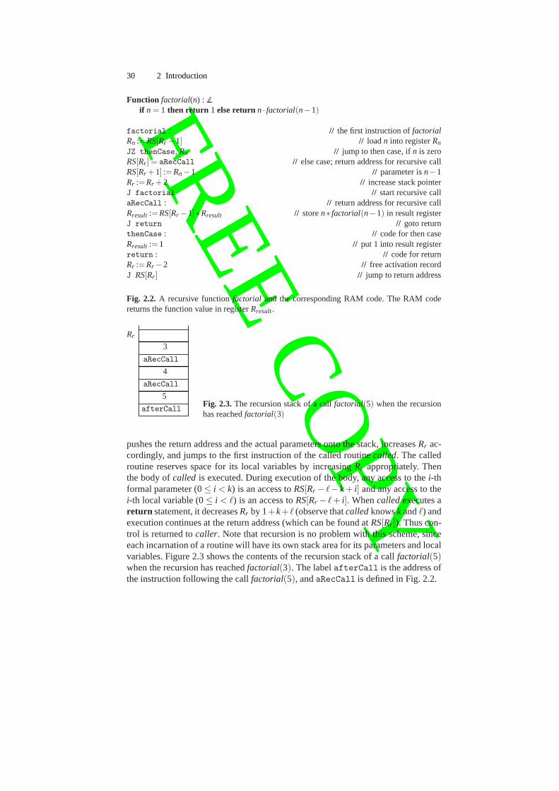
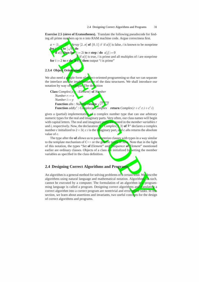
Functionsare similar to procedures, except that they allow the returnstatement toreturn a value. Figure 2.2 shows the declaration of a recursive function that returnsn!and its translation into RAM code. The substitution approach fails for recursivepro-cedures and functions that directly or indirectly call themselves – substitution wouldnever terminate. Realizing recursive procedures in RAM code requires the conceptof a recursion stack. Explicit subroutine calls over a stack are also used for largeprocedures that are called multiple times where inlining would unduly increase thecode size. The recursion stack is a reserved part of the memory; we useRSto denoteit. RScontains a sequence ofactivation records, one for each active procedure call.A special registerRr always points to the first free entry in this stack. The activationrecord for a procedure withk parameters andℓ local variables has size 1+k+ ℓ. Thefirst location contains the return address, i.e., the address of the instruction whereexecution is to be continued after the call has terminated, the nextk locations arereserved for the parameters, and the finalℓ locations are for the local variables. Aprocedure call is now implemented as follows. First, the calling procedurecaller

FRE

EC

OP

Y30 2 Introduction

Function factorial(n) : Zif n = 1 then return 1 else returnn· factorial(n−1)

factorial : // the first instruction offactorialRn :=RS[Rr −1] // loadn into registerRn

JZ thenCase, Rn // jump to then case, ifn is zeroRS[Rr ] = aRecCall // else case; return address for recursive callRS[Rr +1] := Rn−1 // parameter isn−1Rr :=Rr +2 // increase stack pointerJ factorial // start recursive callaRecCall : // return address for recursive callRresult :=RS[Rr −1]∗Rresult // storen∗ factorial(n−1) in result registerJ return // goto returnthenCase : // code for then caseRresult :=1 // put 1 into result registerreturn : // code for returnRr :=Rr −2 // free activation recordJ RS[Rr ] // jump to return address

Fig. 2.2. A recursive functionfactorial and the corresponding RAM code. The RAM codereturns the function value in registerRresult.

aRecCall

aRecCall

afterCall

5

4

3

Rr

Fig. 2.3.The recursion stack of a callfactorial(5) when the recursionhas reachedfactorial(3)

pushes the return address and the actual parameters onto thestack, increasesRr ac-cordingly, and jumps to the first instruction of the called routinecalled. The calledroutine reserves space for its local variables by increasing Rr appropriately. Thenthe body ofcalled is executed. During execution of the body, any access to thei-thformal parameter (0≤ i < k) is an access toRS[Rr − ℓ−k+ i] and any access to thei-th local variable (0≤ i < ℓ) is an access toRS[Rr − ℓ+ i]. Whencalledexecutes areturn statement, it decreasesRr by 1+k+ℓ (observe thatcalledknowsk andℓ) andexecution continues at the return address (which can be found atRS[Rr ]). Thus con-trol is returned tocaller. Note that recursion is no problem with this scheme, sinceeach incarnation of a routine will have its own stack area forits parameters and localvariables. Figure 2.3 shows the contents of the recursion stack of a callfactorial(5)when the recursion has reachedfactorial(3). The labelafterCall is the address ofthe instruction following the callfactorial(5), andaRecCall is defined in Fig. 2.2.

FRE

EC

OP

Y2.4 Designing Correct Algorithms and Programs 31

Exercise 2.5 (sieve of Eratosthenes).Translate the following pseudocode for find-ing all prime numbers up ton into RAM machine code. Argue correctness first.

a = 〈1, . . . ,1〉 : Array [2..n] of 0,1 // if a[i] is false,i is known to be nonprimefor i :=2 to ⌊√n⌋ do

if a[i] then for j :=2i to n step i do a[ j] :=0// if a[i] is true,i is prime and all multiples ofi are nonprime

for i :=2 to n do if a[i] then output “i is prime”

2.3.4 Object Orientation

We also need a simple form of object-oriented programming sothat we can separatethe interface and the implementation of the data structures. We shall introduce ournotation by way of example. The definition

ClassComplex(x,y : Element) of NumberNumber r:=xNumber i:=yFunction abs: Numberreturn

√r2 + i2

Function add(c′ : Complex) : Complex return Complex(r +c′.r, i +c′.i)

gives a (partial) implementation of a complex number type that can use arbitrarynumeric types for the real and imaginary parts. Very often, our class names will beginwith capital letters. The real and imaginary parts are stored in themember variables randi, respectively. Now, the declaration “c : Complex(2,3) of R” declares a complexnumberc initialized to 2+3i; c.i is the imaginary part, andc.absreturns the absolutevalue ofc.

The type after theof allows us to parameterize classes with types in a way similarto the template mechanism of C++ or the generic types of Java. Note that in the lightof this notation, the types “Setof Element” and “Sequenceof Element” mentionedearlier are ordinary classes. Objects of a class are initialized by setting the membervariables as specified in the class definition.

2.4 Designing Correct Algorithms and Programs

An algorithm is a general method for solving problems of a certain kind. We describealgorithms using natural language and mathematical notation. Algorithms, as such,cannot be executed by a computer. The formulation of an algorithm in a program-ming language is called a program. Designing correct algorithms and translating acorrect algorithm into a correct program are nontrivial anderror-prone tasks. In thissection, we learn about assertions and invariants, two useful concepts for the designof correct algorithms and programs.

FRE

EC

OP

Y32 2 Introduction

2.4.1 Assertions and Invariants

Assertionsand invariantsdescribe properties of the program state, i.e., propertiesof single variables and relations between the values of several variables. Typicalproperties are that a pointer has a defined value, an integer is nonnegative, a listis nonempty, or the value of an integer variablelength is equal to the length of acertain listL. Figure 2.4 shows an example of the use of assertions and invariantsin a functionpower(a,n0) that computesan0 for a real numbera and a nonnegativeintegern0.

We start with the assertionassertn0 ≥ 0 and¬(a = 0∧n0 = 0). This states thatthe program expects a nonnegative integern0 and that not bothaandn0 are allowed tobe zero. We make no claim about the behavior of our program forinputs that violatethis assertion. This assertion is therefore called thepreconditionof the program.It is good programming practice to check the precondition ofa program, i.e., towrite code which checks the precondition and signals an error if it is violated. Whenthe precondition holds (and the program is correct), apostconditionholds at thetermination of the program. In our example, we assert thatr = an0. It is also goodprogramming practice to verify the postcondition before returning from a program.We shall come back to this point at the end of this section.

One can view preconditions and postconditions as acontractbetween the callerand the called routine: if the caller passes parameters satisfying the precondition, theroutine produces a result satisfying the postcondition.

For conciseness, we shall use assertions sparingly, assuming that certain “ob-vious” conditions are implicit from the textual description of the algorithm. Muchmore elaborate assertions may be required for safety-critical programs or for formalverification.

Preconditions and postconditions are assertions that describe the initial and thefinal state of a program or function. We also need to describe properties of interme-diate states. Some particularly important consistency properties should hold at manyplaces in a program. These properties are calledinvariants. Loop invariants and datastructure invariants are of particular importance.

Function power(a : R; n0 : N) : Rassertn0 ≥ 0 and¬(a = 0∧n0 = 0) // It is not so clear what 00 should bep = a : R; r = 1 :R; n = n0 : N // we have:pnr = an0

while n > 0 doinvariant pnr = an0

if n is oddthen n--; r := r · p // invariant violated between assignmentselse(n, p) :=(n/2, p· p) // parallel assignment maintains invariant

assertr = an0 // This is a consequence of the invariant andn = 0return r

Fig. 2.4.An algorithm that computes integer powers of real numbers.

FRE

EC

OP

Y2.4 Designing Correct Algorithms and Programs 33

2.4.2 Loop Invariants

A loop invariantholds before and after each loop iteration. In our example, we claimthat pnr = an0 before each iteration. This is true before the first iteration. The ini-tialization of the program variables takes care of this. In fact, an invariant frequentlytells us how to initialize the variables. Assume that the invariant holds before exe-cution of the loop body, andn > 0. If n is odd, we decrementn and multiplyr byp. This reestablishes the invariant (note that the invariantis violated between the as-signments). Ifn is even, we halven and squarep, and again reestablish the invariant.When the loop terminates, we havepnr = an0 by the invariant, andn = 0 by thecondition of the loop. Thusr = an0 and we have established the postcondition.

The algorithm in Fig. 2.4 and many more algorithms describedin this book havea quite simple structure. A few variables are declared and initialized to establishthe loop invariant. Then, a main loop manipulates the state of the program. When theloop terminates, the loop invariant together with the termination condition of the loopimplies that the correct result has been computed. The loop invariant therefore playsa pivotal role in understanding why a program works correctly. Once we understandthe loop invariant, it suffices to check that the loop invariant is true initially and aftereach loop iteration. This is particularly easy if the loop body consists of only a smallnumber of statements, as in the example above.

2.4.3 Data Structure Invariants

More complex programs encapsulate their state in objects whose consistent repre-sentation is also governed by invariants. Suchdata structure invariantsare declaredtogether with the data type. They are true after an object is constructed, and theyare preconditions and postconditions of all methods of a class. For example, weshall discuss the representation of sets by sorted arrays. The data structure invari-ant will state that the data structure uses an arraya and an integern, thatn is the sizeof a, that the setS stored in the data structure is equal toa[1], . . . ,a[n], and thata[1] < a[2] < .. . < a[n]. The methods of the class have to maintain this invariant andthey are allowed to leverage the invariant; for example, thesearch method may makeuse of the fact that the array is sorted.

2.4.4 Certifying Algorithms

We mentioned above that it is good programming practice to check assertions. Itis not always clear how to do this efficiently; in our example program, it is easy tocheck the precondition, but there seems to be no easy way to check the postcondition.In many situations, however,the task of checking assertions can be simplified bycomputing additional information. This additional information is called acertificateorwitness, and its purpose is to simplify the check of an assertion. When an algorithmcomputes a certificate for the postcondition, we call it acertifying algorithm. Weshall illustrate the idea by an example. Consider a functionwhose input is a graphG = (V,E). Graphs are defined in Sect. 2.9. The task is to test whether the graph is

FRE

EC

OP

Y34 2 Introduction

bipartite, i.e., whether there is a labeling of the nodes ofG with the colors blue andred such that any edge ofG connects nodes of different colors. As specified so far,the function returns true or false – true ifG is bipartite, and false otherwise. With thisrudimentary output, the postcondition cannot be checked. However, we may augmentthe program as follows. When the program declaresG bipartite, it also returns a two-coloring of the graph. When the program declaresG nonbipartite, it also returns acycle of odd length in the graph. For the augmented program, the postcondition iseasy to check. In the first case, we simply check whether all edges connect nodes ofdifferent colors, and in the second case, we do nothing. An odd-length cycle provesthat the graph is nonbipartite. Most algorithms in this bookcan be made certifyingwithout increasing the asymptotic running time.

2.5 An Example – Binary Search

Binary search is a very useful technique for searching in an ordered set of items. Weshall use it over and over again in later chapters.

The simplest scenario is as follows. We are given a sorted array a[1..n] of pair-wise distinct elements, i.e.,a[1] < a[2] < .. . < a[n], and an elementx. Now we arerequired to find the indexi with a[i −1] < x≤ a[i]; here,a[0] anda[n+1] should beinterpreted as fictitious elements with values−∞ and+∞, respectively. We can usethese fictitious elements in the invariants and the proofs, but cannot access them inthe program.

Binary search is based on the principle of divide-and-conquer. We choose anindexm∈ [1..n] and comparex with a[m]. If x = a[m], we are done and returni = m.If x< a[m], we restrict the search to the part of the array beforea[m], and ifx> a[m],we restrict the search to the part of the array aftera[m]. We need to say more clearlywhat it means to restrict the search to a subinterval. We havetwo indicesℓ andr, andmaintain the invariant

(I) 0≤ ℓ < r ≤ n+1 and a[ℓ] < x < a[r] .

This is true initially withℓ = 0 andr = n+1. If ℓ andr are consecutive indices,x isnot contained in the array. Figure 2.5 shows the complete program.

The comments in the program show that the second part of the invariant is main-tained. With respect to the first part, we observe that the loop is entered withℓ < r.If ℓ+1= r, we stop and return. Otherwise,ℓ+2≤ r and henceℓ < m< r. Thusm isa legal array index, and we can accessa[m]. If x = a[m], we stop. Otherwise, we seteitherr = m or ℓ = mand hence haveℓ < r at the end of the loop. Thus the invariantis maintained.

Let us argue for termination next. We observe first that if an iteration is not thelast one, then we either increaseℓ or decreaser, and hencer − ℓ decreases. Thus thesearch terminates. We want to show more. We want to show that the search terminatesin a logarithmic number of steps. To do this, we study the quantity r − ℓ−1. Notethat this is the number of indicesi with ℓ < i < r, and hence a natural measure of the

FRE

EC

OP

Y2.5 An Example – Binary Search 35

size of the current subproblem. We shall show that each iteration except the last atleast halves the size of the problem. If an iteration is not the last,r − ℓ−1 decreasesto something less than or equal to

maxr −⌊(r + ℓ)/2⌋−1,⌊(r + ℓ)/2⌋− ℓ−1≤ maxr − ((r + ℓ)/2−1/2)−1,(r + ℓ)/2− ℓ−1= max(r − ℓ−1)/2,(r − ℓ)/2−1= (r − ℓ−1)/2 ,

and hence it at least halved. We start withr − ℓ−1 = n+ 1−0−1= n, and hencehaver − ℓ−1≤

⌊

n/2k⌋

afterk iterations. The(k+1)-th iteration is certainly the lastif we enter it withr = ℓ+1. This is guaranteed ifn/2k < 1 ork > logn. We concludethat, at most, 2+ logn iterations are performed. Since the number of comparisons isa natural number, we can sharpen the bound to 2+ ⌊logn⌋.Theorem 2.3.Binary search finds an element in a sorted array of size n in2+⌊logn⌋comparisons between elements.

Exercise 2.6.Show that the above bound is sharp, i.e., for everyn there are instanceswhere exactly 2+ ⌊logn⌋ comparisons are needed.

Exercise 2.7.Formulate binary search with two-way comparisons, i.e., distinguishbetween the casesx < a[m], andx≥ a[m].

We next discuss two important extensions of binary search. First, there is no needfor the valuesa[i] to be stored in an array. We only need the capability to computea[i], giveni. For example, if we have a strictly monotonic functionf and argumentsiand j with f (i) < x< f ( j), we can use binary search to findmsuch thatf (m) ≤ x<f (m+1). In this context, binary search is often referred to as thebisection method.

Second, we can extend binary search to the case where the array is infinite. As-sume we have an infinite arraya[1..∞] with a[1] ≤ x and want to findm such thata[m] ≤ x < a[m+ 1]. If x is larger than all elements in the array, the procedure isallowed to diverge. We proceed as follows. We comparex with a[21], a[22], a[23],. . . , until the firsti with x< a[2i] is found. This is called anexponential search. Thenwe complete the search by binary search on the arraya[2i−1..2i ].

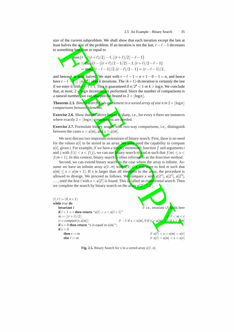
(ℓ, r) :=(0,n+1)while true do

invariant I // i.e., invariant(I) holds hereif ℓ+1 = r then return “a [ℓ] < x < a[ℓ+1]”m:= ⌊(r + ℓ)/2⌋ // ℓ < m< rs:=compare(x,a[m]) // −1 if x < a[m], 0 if x = a[m], +1 if x > a[m]if s= 0 then return “x is equal to a[m]”;if s< 0

then r :=m // a[ℓ] < x < a[m] = a[r]elseℓ :=m // a[ℓ] = a[m] < x < a[r]

Fig. 2.5.Binary Search forx in a sorted arraya[1..n].

FRE

EC

OP

Y36 2 Introduction

Theorem 2.4.The combination of exponential and binary search finds x in anun-bounded sorted array in at most2logm+3 comparisons, where a[m]≤ x< a[m+1].

Proof. We needi comparisons to find the firsti such thatx < a[2i], followed bylog(2i −2i−1)+2 comparisons for the binary search. This gives a total of 2i + 1comparisons. Sincem≥ 2i−1, we havei ≤ 1+ logmand the claim follows. ⊓⊔

Binary search is certifying. It returns an indexm with a[m] ≤ x < a[m+ 1]. Ifx = a[m], the index proves thatx is stored in the array. Ifa[m] < x < a[m+ 1] andthe array is sorted, the index proves thatx is not stored in the array. Of course, if thearray violates the precondition and is not sorted, we know nothing. There is no wayto check the precondition in logarithmic time.

2.6 Basic Algorithm Analysis

Let us summarize the principles of algorithm analysis. We abstract from the compli-cations of a real machine to the simplified RAM model. In the RAM model, runningtime is measured by the number of instructions executed. We simplify the analy-sis further by grouping inputs by size and focusing on the worst case. The use ofasymptotic notation allows us to ignore constant factors and lower-order terms. Thiscoarsening of our view also allows us to look at upper bounds on the execution timerather than the exact worst case, as long as the asymptotic result remains unchanged.The total effect of these simplifications is that the runningtime of pseudocode can beanalyzed directly. There is no need to translate the programinto machine code first.

We shall next introduce a set of simple rules for analyzing pseudocode. LetT(I)denote the worst-case execution time of a piece of programI . The following rulesthen tell us how to estimate the running time for larger programs, given that we knowthe running times of their constituents:

• T(I ; I ′) = T(I)+T(I ′).• T(if C then I elseI ′) = O(T(C)+max(T(I),T(I ′))).• T(repeat I until C) = O

(

∑ki=1T(i)

)

, wherek is the number of loop iterations,andT(i) is the time needed in thei-th iteration of the loop, including the testC.

We postpone the treatment of subroutine calls to Sect. 2.6.2. Of the rules above, onlythe rule for loops is nontrivial to apply; it requires evaluating sums.

2.6.1 “Doing Sums”

We now introduce some basic techniques for evaluating sums.Sums arise in theanalysis of loops, in average-case analysis, and also in theanalysis of randomizedalgorithms.

For example, the insertion sort algorithm introduced in Sect. 5.1 has two nestedloops. The outer loop countsi, from 2 ton. The inner loop performs at mosti − 1iterations. Hence, the total number of iterations of the inner loop is at most

FRE

EC

OP

Y2.6 Basic Algorithm Analysis 37

n

∑i=2

(i −1) =n−1

∑i=1

i =n(n−1)

2= O

(

n2) ,

where the second equality comes from (A.11). Since the time for one execution ofthe inner loop is O(1), we get a worst-case execution time ofΘ

(

n2)

. All nestedloops with an easily predictable number of iterations can beanalyzed in an analogousfashion: work your way outwards by repeatedly finding a closed-form expression forthe innermost loop. Using simple manipulations such as∑i cai = c∑i ai, ∑i(ai +bi)=

∑i ai + ∑i bi, or ∑ni=2ai = −a1 + ∑n

i=1ai , one can often reduce the sums to simpleforms that can be looked up in a catalog of sums. A small sampleof such formulaecan be found in Appendix A. Since we are usually interested only in the asymptoticbehavior, we can frequently avoid doing sums exactly and resort to estimates. Forexample, instead of evaluating the sum above exactly, we mayargue more simply asfollows:

n

∑i=2

(i −1)≤n

∑i=1

n = n2 = O(

n2) ,

n

∑i=2

(i −1)≥n

∑i=⌈n/2⌉

n/2 = ⌊n/2⌋ ·n/2= Ω(

n2) .

2.6.2 Recurrences

In our rules for analyzing programs, we have so far neglectedsubroutine calls. Non-recursive subroutines are easy to handle, since we can analyze the subroutine sepa-rately and then substitute the bound obtained into the expression for the running timeof the calling routine. For recursive programs, however, this approach does not leadto a closed formula, but to a recurrence relation.

For example, for the recursive variant of the school method of multiplica-tion, we obtainedT(1) = 1 andT(n) = 6n+ 4T(⌈n/2⌉) for the number of prim-itive operations. For the Karatsuba algorithm, the corresponding expression wasT(n) = 3n2 + 2n for n≤ 3 andT(n) = 12n+ 3T(⌈n/2⌉+ 1) otherwise. In general,a recurrence relationdefines a function in terms of the same function using smallerarguments. Explicit definitions for small parameter valuesmake the function welldefined. Solving recurrences, i.e., finding nonrecursive, closed-form expressions forthem, is an interesting subject in mathematics. Here we focus on the recurrence re-lations that typically emerge from divide-and-conquer algorithms. We begin with asimple case that will suffice for the purpose of understanding the main ideas. Wehave a problem of sizen = bk for some integerk. If k > 1, we invest linear workcnin dividing the problem intod subproblems of sizen/b and combining the results. Ifk = 0, there are no recursive calls, we invest worka, and are done.

Theorem 2.5 (master theorem (simple form)).For positive constants a, b, c, andd, and n= bk for some integer k, consider the recurrence

r(n) =

a if n = 1 ,

cn+d · r(n/b) if n > 1 .

FRE

EC

OP

Y38 2 Introduction

Then

r(n) =

Θ(n) if d < b ,

Θ(nlogn) if d = b ,

Θ(

nlogb d)

if d > b .

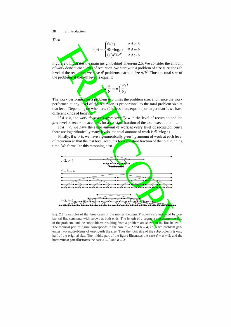
Figure 2.6 illustrates the main insight behind Theorem 2.5.We consider the amountof work done at each level of recursion. We start with a problem of sizen. At the i-thlevel of the recursion, we havedi problems, each of sizen/bi. Thus the total size ofthe problems at thei-th level is equal to

di nbi = n

(

db

)i

.

The work performed for a problem isc times the problem size, and hence the workperformed at any level of the recursion is proportional to the total problem size atthat level. Depending on whetherd/b is less than, equal to, or larger than 1, we havedifferent kinds of behavior.

If d < b, the workdecreases geometricallywith the level of recursion and thefirst level of recursion accounts for a constant fraction of the total execution time.

If d = b, we have the same amount of work ateverylevel of recursion. Sincethere are logarithmically many levels, the total amount of work is Θ(nlogn).

Finally, if d > b, we have a geometricallygrowingamount of work at each levelof recursion so that thelast level accounts for a constant fraction of the total runningtime. We formalize this reasoning next.

d=2, b=4

d=3, b=2

d = b = 4

Fig. 2.6.Examples of the three cases of the master theorem. Problems are indicated by hor-izontal line segments with arrows at both ends. The length ofa segment represents the sizeof the problem, and the subproblems resulting from a problemare shown in the line below it.The topmost part of figure corresponds to the cased = 2 andb = 4, i.e., each problem gen-erates two subproblems of one-fourth the size. Thus the total size of the subproblems is onlyhalf of the original size. The middle part of the figure illustrates the cased = b = 2, and thebottommost part illustrates the cased = 3 andb = 2

FRE

EC

OP

Y2.6 Basic Algorithm Analysis 39

Proof. We start with a single problem of sizen = bk. W call this level zero of therecursion.3 At level 1, we haved problems, each of sizen/b = bk−1. At level 2, wehaved2 problems, each of sizen/b2 = bk−2. At level i, we havedi problems, eachof sizen/bi = bk−i . At level k, we havedk problems, each of sizen/bk = bk−k = 1.Each such problem has a costa, and hence the total cost at levelk is adk.

Let us next compute the total cost of the divide-and-conquersteps at levels 1 tok−1. At level i, we havedi recursive calls each for subproblems of sizebk−i . Eachcall contributes a cost ofc ·bk−i , and hence the cost at leveli is di ·c ·bk−i . Thus thecombined cost over all levels is

k−1

∑i=0

di ·c ·bk−i = c ·bk ·k−1

∑i=0

(

db

)i

= cn·k−1

∑i=0

(

db

)i

.

We now distinguish cases according to the relative sizes ofd andb.

Cased = b. We have a costadk = abk = an= Θ(n) for the bottom of the recursionandcnk= cnlogb n = Θ(nlogn) for the divide-and-conquer steps.

Cased < b. We have a costadk < abk = an= O(n) for the bottom of the recursion.For the cost of the divide-and-conquer steps, we use (A.13) for a geometric series,namely∑0≤i<k xi = (1−xk)/(1−x) for x > 0 andx 6= 1, and obtain

cn·k−1

∑i=0

(

db

)i

= cn· 1− (d/b)k

1−d/b< cn· 1

1−d/b= O(n)

and

cn·k−1

∑i=0

(

db

)i

= cn· 1− (d/b)k

1−d/b> cn= Ω(n) .

Cased > b. First, note that

dk = 2k logd = 2k logblogb logd

= bk logdlogb = bk logb d = nlogbd .

Hence the bottom of the recursion has a cost ofanlogb d = Θ(

nlogb d)

. For the divide-and-conquer steps we use the geometric series again and obtain

cbk (d/b)k−1d/b−1

= cdk−bk

d/b−1= cdk 1− (b/d)k

d/b−1= Θ

(

dk)

= Θ(

nlogbd)

.⊓⊔

We shall use the master theorem many times in this book. Unfortunately, the re-currenceT(n) = 3n2 + 2n for n ≤ 3 andT(n) ≤ 12n+ 3T(⌈n/2⌉+ 1), governing

3 In this proof, we use the terminology of recursive programs in order to give an intuitiveidea of what we are doing. However, our mathematical arguments apply to any recurrencerelation of the right form, even if it does not stem from a recursive program.

FRE

EC

OP

Y40 2 Introduction

Karatsuba’s algorithm, is not covered by our master theorem, which neglects round-ing issues. We shall now show how to extend the master theoremto the followingrecurrence:

r(n) ≤

a if n≤ n0,

cn+d · r(⌈n/b⌉+e) if n > n0,

wherea, b, c, d, andeare constants, andn0 is such that⌈n/b⌉+e< n for n> n0. Weproceed in two steps. We first concentrate onn of the formbk+z, wherez is such that⌈z/b⌉+e= z. For example, forb= 2 ande= 3, we would choosez= 6. Note that forn of this form, we have⌈n/b⌉+e=

⌈

(bk +z)/b⌉

+e= bk−1 + ⌈z/b⌉+e= bk−1+z,i.e., the reduced problem size has the same form. For then’s in this special form, wethen argue exactly as in Theorem 2.5.

How do we generalize to arbitraryn? The simplest way is semantic reasoning. Itis clear4 that the cost grows with the problem size, and hence the cost for an input ofsizen will be no larger than the cost for an input whose size is equalto the next inputsize of special form. Since this input is at mostb times larger andb is a constant, thebound derived for specialn is affected only by a constant factor.

The formal reasoning is as follows (you may want to skip this paragraph andcome back to it when the need arises). We define a functionR(n) by the same recur-rence, with≤ replaced by equality:R(n) = a for n≤ n0 andR(n) = cn+dR(⌈n/b⌉+e) for n > n0. Obviously,r(n) ≤ R(n). We derive a bound forR(n) andn of specialform as described above. Finally, we argue by induction thatR(n) ≤ R(s(n)), wheres(n) is the smallest number of the formbk +zwith bk +z≥ n. The induction step isas follows:

R(n) = cn+dR(⌈n/b⌉+e) ≤ cs(n)+dR(s(⌈n/b⌉+e)) = R(s(n)) ,

where the inequality uses the induction hypothesis andn ≤ s(n). The last equalityuses the fact that fors(n) = bk + z (and hencebk−1 + z < n), we havebk−2 + z <⌈n/b⌉+e≤ bk−1 +zand hences(⌈n/b⌉+e) = bk−1 +z= ⌈s(n)/b⌉+e.

There are many generalizations of the master theorem: we might break the re-cursion earlier, the cost for dividing and conquering may benonlinear, the size ofthe subproblems might vary within certain bounds, the number of subproblems maydepend on the input size, etc. We refer the reader to the books[81, 175] for furtherinformation.

Exercise 2.8.Consider the recurrence

C(n) =

1 if n = 1,

C(⌊n/2⌋)+C(⌈n/2⌉)+cn if n > 1.

Show thatC(n) = O(nlogn).

4 Be aware that most errors in mathematical arguments are nearoccurrences of the word“clearly”.

FRE

EC

OP

Y2.7 Average-Case Analysis 41

*Exercise 2.9.Suppose you have a divide-and-conquer algorithm whose runningtime is governed by the recurrenceT(1) = a, T(n) = cn+ ⌈√n ⌉T(⌈n/⌈√n ⌉⌉).Show that the running time of the program is O(nloglogn).

Exercise 2.10.Access to data structures is often governed by the followingrecur-rence:T(1) = a, T(n) = c+T(n/2). Show thatT(n) = O(logn).

2.6.3 Global Arguments

The algorithm analysis techniques introduced so far are syntax-oriented in the fol-lowing sense: in order to analyze a large program, we first analyze its parts and thencombine the analyses of the parts into an analysis of the large program. The combi-nation step involves sums and recurrences.

We shall also use a completely different approach which one might call semantics-oriented. In this approach we associate parts of the execution with parts of a combi-natorial structure and then argue about the combinatorial structure. For example, wemight argue that a certain piece of program is executed at most once for each edgeof a graph or that the execution of a certain piece of program at least doubles the sizeof a certain structure, that the size is one initially, and atmostn at termination, andhence the number of executions is bounded logarithmically.

2.7 Average-Case Analysis

In this section we shall introduce you to average-case analysis. We shall do so byway of three examples of increasing complexity. We assume that you are familiarwith basic concepts of probability theory such as discrete probability distributions,expected values, indicator variables, and the linearity ofexpectations. Section A.3reviews the basics.

2.7.1 Incrementing a Counter

We begin with a very simple example. Our input is an arraya[0..n− 1] filled withdigits zero and one. We want to increment the number represented by the array byone.

i :=0while (i < n and a[i] = 1) do a[i] = 0; i++;if i < n then a[i] = 1

How often is the body of the while loop executed? Clearly,n times in the worstcase and 0 times in the best case. What is the average case? Thefirst step in anaverage-case analysis is always to define the model of randomness, i.e., to define theunderlying probability space. We postulate the following model of randomness: eachdigit is zero or one with probability 1/2, and different digits are independent. Theloop body is executedk times, 0≤ k ≤ n, iff the lastk+ 1 digits ofa are 01k or k

FRE

EC

OP

Y42 2 Introduction

is equal ton and all digits ofa are equal to one. The former event has probability2−(k+1), and the latter event has probability 2−n. Therefore, the average number ofexecutions is equal to

∑0≤k<n

k2−(k+1) +n2−n ≤ ∑k≥0

k2−k = 2 ,

where the last equality is the same as (A.14).

2.7.2 Left-to-Right Maxima

Our second example is slightly more demanding. Consider thefollowing simple pro-gram that determines the maximum element in an arraya[1..n]:

m:=a[1]; for i :=2 to n do if a[i] > m then m:=a[i]

How often is the assignmentm:=a[i] executed? In the worst case, it is executed inevery iteration of the loop and hencen−1 times. In the best case, it is not executedat all. What is the average case? Again, we start by defining the probability space.We assume that the array containsn distinct elements and that any order of theseelements is equally likely. In other words, our probabilityspace consists of then!permutations of the array elements. Each permutation is equally likely and thereforehas probability 1/n!. Since the exact nature of the array elements is unimportant,we may assume that the array contains the numbers 1 ton in some order. We areinterested in the average number ofleft-to-right maxima. A left-to-right maximum ina sequence is an element which is larger than all preceding elements. So,(1,2,4,3)has three left-to-right-maxima and(3,1,2,4) has two left-to-right-maxima. For apermutationπ of the integers 1 ton, letMn(π) be the number of left-to-right-maxima.What is E[Mn]? We shall describe two ways to determine the expectation. For smalln, is easy to determine E[Mn] by direct calculation. Forn = 1, there is only onepermutation, namely(1), and it has one maximum. So E[M1] = 1. Forn = 2, thereare two permutations, namely(1,2) and(2,1). The former has two maxima and thelatter has one maximum. So E[M2] = 1.5. For largern, we argue as follows.

We write Mn as a sum of indicator variablesI1 to In, i.e., Mn = I1 + . . . + In,whereIk is equal to one for a permutationπ if the k-th element ofπ is a left-to-rightmaximum. For example,I3((3,1,2,4)) = 0 andI4((3,1,2,4)) = 1. We have

E[Mn] = E[I1 + I2+ . . .+ In]

= E[I1]+E[I2]+ . . .+E[In]

= prob(I1 = 1)+prob(I2 = 1)+ . . .+prob(In = 1) ,

where the second equality is the linearity of expectations (A.2) and the third equalityfollows from theIk’s being indicator variables. It remains to determine the probabil-ity that Ik = 1. Thek-th element of a random permutation is a left-to-right maximumif and only if thek-th element is the largest of the firstk elements. In a random per-mutation, any position is equally likely to hold the maximum, so that the probabilitywe are looking for is prob(Ik = 1) = 1/k and hence

FRE

EC

OP

Y2.7 Average-Case Analysis 43

E[Mn] = ∑1≤k≤n

prob(Ik = 1) = ∑1≤k≤n

1k

.

So, E[M4] = 1+1/2+1/3+1/4=(12+6+4+3)/12= 25/12.The sum∑1≤k≤n1/kwill appear several times in this book. It is known under the name “n-th harmonicnumber” and is denoted byHn. It is known that lnn≤ Hn ≤ 1+ lnn, i.e.,Hn ≈ lnn;see (A.12). We conclude that the average number of left-to-right maxima is muchsmaller than in the worst case.

Exercise 2.11.Show thatn

∑k=1

1k≤ lnn+1. Hint: show first that

n

∑k=2

1k≤∫ n

1

1x

dx.

We now describe an alternative analysis. We introduceAn as a shorthand forE[Mn] and setA0 = 0. The first element is always a left-to-right maximum, and eachnumber is equally likely as the first element. If the first element is equal toi, then onlythe numbersi + 1 to n can be further left-to-right maxima. They appear in randomorder in the remaining sequence, and hence we shall see an expected number ofAn−i

further maxima. Thus

An = 1+

(

∑1≤i≤n

An−i

)

/n or nAn = n+ ∑0≤i≤n−1

Ai .

A simple trick simplifies this recurrence. The corresponding equation forn− 1 in-stead ofn is (n−1)An−1 = n−1+ ∑1≤i≤n−2Ai . Subtracting the equation forn−1from the equation forn yields

nAn− (n−1)An−1 = 1+An−1 or An = 1/n+An−1 ,

and henceAn = Hn.

2.7.3 Linear Search

We come now to our third example; this example is even more demanding. Considerthe following search problem. We have items 1 ton, which we are required to arrangelinearly in some order; say, we put itemi in positionℓi . Once we have arranged theitems, we perform searches. In order to search for an itemx, we go through thesequence from left to right until we encounterx. In this way, it will takeℓi steps toaccess itemi.

Suppose now that we also know that we shall access the items with differentprobabilities; say, we search for itemi with probability pi , wherepi ≥ 0 for all i,1 ≤ i ≤ n, and∑i pi = 1. In this situation, theexpectedor averagecost of a searchis equal to∑i piℓi , since we search for itemi with probability pi and the cost of thesearch isℓi .

What is the best way of arranging the items? Intuition tells us that we shouldarrange the items in order of decreasing probability. Let usprove this.

FRE

EC

OP

Y44 2 Introduction

Lemma 2.6.An arrangement is optimal with respect to the expected search cost if ithas the property that pi > p j impliesℓi < ℓ j . If p1 ≥ p2 ≥ . . . ≥ pn, the placementℓi = i results in the optimal expected search cost Opt= ∑i pi i.

Proof. Consider an arrangement in which, for somei and j, we havepi > p j andℓi > ℓ j , i.e., itemi is more probable than itemj and yet placed after it. Interchangingitemsi and j changes the search cost by

−(piℓi + p jℓ j)+ (piℓ j + p jℓi) = (pi − p j)(ℓi − ℓ j) < 0 ,

i.e., the new arrangement is better and hence the old arrangement is not optimal.Let us now consider the casep1 > p2 > .. . > pn. Since there are onlyn! possible

arrangements, there is an optimal arrangement. Also, ifi < j and i is placed afterj, the arrangement is not optimal by the argument in the preceding paragraph. Thusthe optimal arrangement puts itemi in positionℓi = i and its expected search cost is∑i pi i.

If p1 ≥ p2 ≥ . . . ≥ pn, the arrangementℓi = i for all i is still optimal. However,if some probabilities are equal, we have more than one optimal arrangement. Withinblocks of equal probabilities, the order is irrelevant. ⊓⊔

Can we still do something intelligent if the probabilitiespi are not known to us?The answer is yes, and a very simple heuristic does the job. Itis called themove-to-front heuristic. Suppose we access itemi and find it in positionℓi . If ℓi = 1, we arehappy and do nothing. Otherwise, we place it in position 1 andmove the items inpositions 1 toℓi −1 one position to the rear. The hope is that, in this way, frequentlyaccessed items tend to stay near the front of the arrangementand infrequently ac-cessed items move to the rear. We shall now analyze the expected behavior of themove-to-front heuristic.

Consider two itemsi and j and suppose that both of them were accessed in thepast. Itemi will be accessed before itemj if the last access to itemi occurred after thelast access to itemj. Thus the probability that itemi is before itemj is pi/(pi + p j).With probabilityp j/(pi + p j), item j stands before itemi.

Now, ℓi is simply one plus the number of elements beforei in the list. Thusthe expected value ofℓi is equal to 1+ ∑ j ; j 6=i p j/(pi + p j), and hence the expectedsearch cost in the move-to-front heuristic is

CMTF = ∑i

pi

(

1+ ∑j ; j 6=i

p j

pi + p j

)

= ∑i

pi + ∑i, j ; i 6= j

pi p j

pi + p j.

Observe that for eachi and j with i 6= j, the termpi p j/(pi + p j) appears twice inthe sum above. In order to proceed with the analysis, we assume p1 ≥ p2 ≥ . . . ≥ pn.This is an assumption used in the analysis, the algorithm hasno knowledge of this.Then

FRE

EC

OP

Y2.8 Randomized Algorithms 45

CMTF = ∑i

pi +2 ∑j ; j<i

pi p j

pi + p j= ∑

i

pi

(

1+2 ∑j ; j<i

p j

pi + p j

)

≤ ∑i

pi

(

1+2 ∑j ; j<i

1

)

< ∑i

pi2i = 2∑i

pi i = 2Opt .

Theorem 2.7.The move-to-front heuristic achieves an expected search time which isat most twice the optimum.

2.8 Randomized Algorithms

Suppose you are offered the chance to participate in a TV gameshow. There are 100boxes that you can open in an order of your choice. Boxi contains an amountmi ofmoney. This amount is unknown to you but becomes known once the box is opened.No two boxes contain the same amount of money. The rules of thegame are verysimple:

• At the beginning of the game, the presenter gives you 10 tokens.• When you open a box and the contents of the box are larger than the contents of

all previously opened boxes, you have to hand back a token.5

• When you have to hand back a token but have no tokens, the game ends and youlose.

• When you manage to open all of the boxes, you win and can keep all the money.

There are strange pictures on the boxes, and the presenter gives hints by suggestingthe box to be opened next. Your aunt, who is addicted to this show, tells you thatonly a few candidates win. Now, you ask yourself whether it isworth participatingin this game. Is there a strategy that gives you a good chance of winning? Are thepresenter’s hints useful?

Let us first analyze the obvious algorithm – you always followthe presenter.The worst case is that he makes you open the boxes in order of increasing value.Whenever you open a box, you have to hand back a token, and whenyou open the11th box you are dead. The candidates and viewers would hate the presenter andhe would soon be fired. Worst-case analysis does not give us the right informationin this situation. The best case is that the presenter immediately tells you the bestbox. You would be happy, but there would be no time to place advertisements, sothat the presenter would again be fired. Best-case analysis also does not give us theright information in this situation. We next observe that the game is really the left-to-right maxima question of the preceding section in disguise.You have to hand backa token whenever a new maximum shows up. We saw in the preceding section thatthe expected number of left-to-right maxima in a random permutation isHn, then-thharmonic number. Forn= 100,Hn < 6. So if the presenter were to point to the boxes

5 The contents of the first box opened are larger than the contents of all previously openedboxes, and hence the first token goes back to the presenter in the first round.

FRE

EC

OP

Y46 2 Introduction

in random order, you would have to hand back only 6 tokens on average. But whyshould the presenter offer you the boxes in random order? He has no incentive tohave too many winners.

The solution is to take your fate into your own hands:open the boxes in randomorder. You select one of the boxes at random, open it, then choose a random box fromthe remaining ones, and so on. How do you choose a random box? When there arekboxes left, you choose a random box by tossing a die withk sides or by choosing arandom number in the range 1 tok. In this way, you generate a random permutation ofthe boxes and hence the analysis in the previous section still applies. On average youwill have to return fewer than 6 tokens and hence your 10 tokens suffice. You havejust seen arandomized algorithm. We want to stress that, although the mathematicalanalysis is the same, the conclusions are very different. Inthe average-case scenario,you are at the mercy of the presenter. If he opens the boxes in random order, theanalysis applies; if he does not, it does not. You have no way to tell, except aftermany shows and with hindsight. In other words, the presentercontrols the dice andit is up to him whether he uses fair dice. The situation is completely different in therandomized-algorithms scenario. You control the dice, andyou generate the randompermutation. The analysis is valid no matter what the presenter does.

2.8.1 The Formal Model

Formally, we equip our RAM with an additional instruction:Ri := randInt(C) assignsarandominteger between 0 andC−1 toRi. In pseudocode, we writev:=randInt(C),wherev is an integer variable. The cost of making a random choice is one time unit.Algorithmsnot using randomization are calleddeterministic.

The running time of a randomized algorithm will generally depend on the randomchoices made by the algorithm. So the running time on an instancei is no longer anumber, but a random variable depending on the random choices. We may eliminatethe dependency of the running time on random choices by equipping our machinewith a timer. At the beginning of the execution, we set the timer to a valueT(n),which may depend on the sizen of the problem instance, and stop the machine oncethe timer goes off. In this way, we can guarantee that the running time is bounded byT(n). However, if the algorithm runs out of time, it does not deliver an answer.

The output of a randomized algorithm may also depend on the random choicesmade. How can an algorithm be useful if the answer on an instance i may dependon the random choices made by the algorithm – if the answer maybe “Yes” todayand “No” tomorrow? If the two cases are equally probable, theanswer given by thealgorithm has no value. However, if the correct answer is much more likely than theincorrect answer, the answer does have value. Let us see an example.

Alice and Bob are connected over a slow telephone line. Alicehas an integerxA and Bob has an integerxB, each withnbits. They want to determine whetherthey have the same number. As communication is slow, their goal is to minimize theamount of information exchanged. Local computation is not an issue.

In the obvious solution, Alice sends her number to Bob, and Bob checks whetherthe numbers are equal and announces the result. This requires them to transmitn

FRE

EC

OP

Y2.8 Randomized Algorithms 47

digits. Alternatively, Alice could send the number digit bydigit, and Bob wouldcheck for equality as the digits arrived and announce the result as soon as he knew it,i.e., as soon as corresponding digits differed or all digitshad been transmitted. In theworst case, alln digits have to be transmitted. We shall now show that randomizationleads to a dramatic improvement. After transmission of onlyO(logn) bits, equalityand inequality can be decided with high probability.

Alice and Bob follow the following protocol. Each of them prepares an orderedlist of prime numbers. The list consists of the smallestL primes withk or more bitsand leading bit 1. Each such prime has a value of at least 2k. We shall say moreabout the choice ofL andk below. In this way, it is guaranteed that both Alice andBob generate the same list. Then Alice chooses an indexi, 1≤ i ≤ L, at random andsendsi andxA mod pi to Bob. Bob computesxB mod pi . If xA mod pi 6= xB mod pi ,he declares that the numbers are different. Otherwise, he declares the numbers thesame. Clearly, if the numbers are the same, Bob will say so. Ifthe numbers aredifferent andxA mod pi 6= xB mod pi , he will declare them different. However, ifxA 6= xB and yetxA mod pi = xB mod pi , he will erroneously declare the numbersequal. What is the probability of an error?

An error occurs ifxA 6= xB but xA ≡ xB(modpi). The latter condition is equiv-alent to pi dividing the differenceD = xA − xB. This difference is at most 2n inabsolute value. Since each primepi has a value of at least 2k, our list contains atmostn/k primes that divide6 the difference, and hence the probability of error is atmost(n/k)/L. We can make this probability arbitrarily small by choosingL largeenough. If, say, we want to make the probability less than 0.0000001= 10−6, wechooseL = 106(n/k).

What is the appropriate choice ofk? Out of the numbers withk bits, approxi-mately 2k/k are primes.7 Hence, if 2k/k ≥ 106n/k, the list will contain onlyk-bitintegers. The condition 2k ≥ 106n is tantamount tok ≥ logn+ 6log10. With thischoice ofk, the protocol transmits logL+k = logn+12log10 bits.This is exponen-tially better than the naive protocol.

What can we do if we want an error probability less than 10−12? We could redothe calculations above withL = 1012n. Alternatively, we could run the protocol twiceand declare the numbers different if at least one run declares them different. Thistwo-stage protocol errs only if both runs err, and hence the probability of error is atmost 10−6 ·10−6 = 10−12.

Exercise 2.12.Compare the efficiency of the two approaches for obtaining anerrorprobability of 10−12.

Exercise 2.13.In the protocol described above, Alice and Bob have to prepareridiculously long lists of prime numbers. Discuss the following modified protocol.

6 Let d be the number of primes on our list that divideD. Then 2n ≥ |D| ≥ (2k)d = 2kd andhenced ≤ n/k.

7 For any integerx, let π(x) be the number of primes less than or equal tox. For example,π(10) = 4 because there are four prime numbers (2, 3, 5 and 7) less thanor equal to 10.Then x/(lnx+ 2) < π(x) < x/(lnx− 4) for x ≥ 55. See the Wikipedia entry on “primenumbers” for more information.

FRE

EC

OP

Y48 2 Introduction

Alice chooses a randomk-bit integerp (with leading bit 1) and tests it for primality.If p is not prime, she repeats the process. Ifp is prime, she sendsp andxA mod p toBob.

Exercise 2.14.Assume you have an algorithm which errs with a probability ofatmost 1/4 and that you run the algorithmk times and output the majority output.Derive a bound on the error probability as a function ofk. Do a precise calculationfor k = 2 andk = 3, and give a bound for largek. Finally, determinek such that theerror probability is less than a givenε.

2.8.2 Las Vegas and Monte Carlo Algorithms

Randomized algorithms come in two main varieties, the Las Vegas and the MonteCarlo variety. ALas Vegas algorithmalways computes the correct answer but itsrunning time is a random variable. Our solution for the game show is a Las Vegasalgorithm; it always finds the box containing the maximum; however, the number ofleft-to-right maxima is a random variable. AMonte Carloalgorithm always has thesame run time, but there is a nonzero probability that it gives an incorrect answer. Theprobability that the answer is incorrect is at most 1/4. Our algorithm for comparingtwo numbers over a telephone line is a Monte Carlo algorithm.In Exercise 2.14, it isshown that the error probability can be made arbitrarily small.

Exercise 2.15.Suppose you have a Las Vegas algorithm with an expected executiontimet(n), and that you run it for 4t(n) steps. If it returns an answer within the allotedtime, this answer is returned, otherwise, an arbitrary answer is returned. Show thatthe resulting algorithm is a Monte Carlo algorithm.

Exercise 2.16.Suppose you have a Monte Carlo algorithm with an execution timem(n) that gives a correct answer with probabilityp and a deterministic algorithmthat verifies in timev(n) whether the Monte Carlo algorithm has given the correctanswer. Explain how to use these two algorithms to obtain a Las Vegas algorithmwith expected execution time(m(n)+v(n))/(1− p).

We come back to our game show example. You have 10 tokens available to you.The expected number of tokens required is less than 6. How sure should you be thatyou will go home a winner? We need to bound the probability that Mn is larger than11, because you lose exactly if the sequence in which you order the boxes has 11or more left-to-right maxima.Markov’s inequalityallows you to bound this prob-ability. It states that, for a nonnegative random variableX and any constantc ≥ 1,prob(X ≥ c ·E[X])≤ 1/c; see (A.4) for additional information. We apply the inequal-ity with X = Mn andc = 11/6. We obtain

prob(Mn ≥ 11) ≤ prob

(

Mn ≥116

E[Mn]

)

≤ 611

,

and hence the probability of winning is more than 5/11.

FRE

EC

OP

Y2.9 Graphs 49

2.9 Graphs

Graphs are an extremely useful concept in algorithmics. We use them whenever wewant to model objects and relations between them; in graph terminology, the objectsare callednodes, and the relations between nodes are callededges. Some obviousapplications are to road maps and communication networks, but there are also moreabstract applications. For example, nodes could be tasks tobe completed when build-ing a house, such as “build the walls” or “put in the windows”,and edges could modelprecedence relations such as “the walls have to be built before the windows can beput in”. We shall also see many examples of data structures where it is natural toview objects as nodes and pointers as edges between the object storing the pointerand the object pointed to.

When humans think about graphs, they usually find it convenient to work withpictures showing nodes as bullets and edges as lines and arrows. To treat graphs algo-rithmically, a more mathematical notation is needed: adirected graph G= (V,E) is apair consisting of anode set(or vertex set) V and anedge set(or arc set) E ⊆V ×V.We sometimes abbreviate “directed graph” todigraph. For example, Fig. 2.7 showsthe graphG= (s,t,u,v,w,x,y,z , (s,t), (t,u), (u,v),(v,w),(w,x),(x,y),(y,z),(z,s),(s,v),(z,w),(y,t),(x,u)). Throughout this book, we use the conventionn = |V| andm= |E| if no other definitions forn or mare given. An edgee= (u,v)∈ E representsa connection fromu to v. We callu andv thesourceandtarget, respectively, ofe.We say thate is incidenton u andv and thatv andu areadjacent. The special caseof a self-loop(v,v) is disallowed unless specifically mentioned.

The outdegreeof a nodev is the number of edges leaving it, and itsindegreeis the number of edges ending at it, formally,outdegree(v) = |(v,u) ∈ E| andindegree(v) = |(u,v) ∈ E|. For example, nodew in graphG in Fig. 2.7 has in-degree two and outdegree one.

A bidirected graphis a digraph where, for any edge(u,v), the reverse edge(v,u)is also present. Anundirected graphcan be viewed as a streamlined representation ofa bidirected graph, where we write a pair of edges(u,v), (v,u) as the two-element setu,v. Figure 2.7 shows a three-node undirected graph and its bidirected counterpart.Most graph-theoretic terms for undirected graphs have the same definition as for

self−loop

undirected bidirected

K5

K3,3

v

w

1v

w

1

u

w v

u

w v

u

w v

s

t

x

U

t

u

yz

s

x

1

1

1

1

1

2 −2

2

2

1

1

G

H

Fig. 2.7.Some graphs

FRE

EC

OP

Y50 2 Introduction

their bidirected counterparts, and so this section will concentrate on directed graphsand only mention undirected graphs when there is something special about them.For example, the number of edges of an undirected graph is only half the numberof edges of its bidirected counterpart. Nodes of an undirected graph have identicalindegree and outdegree, and so we simply talk about theirdegree. Undirected graphsare important because directions often do not matter and because many problems areeasier to solve (or even to define) for undirected graphs thanfor general digraphs.

A graphG′ = (V ′,E′) is asubgraphof G if V ′ ⊆V andE′ ⊆ E. GivenG= (V,E)and a subsetV ′ ⊆ V, the subgraphinducedby V ′ is defined asG′ = (V ′,E∩ (V ′×V ′)). In Fig. 2.7, the node setv,w in G induces the subgraphH = (v,w ,(v,w)).A subsetE′ ⊆ E of edges induces the subgraph(V,E′).

Often, additional information is associated with nodes or edges. In particular,we shall often neededge weightsor costs c: E → R that map edges to some numericvalue. For example, the edge(z,w) in graphG in Fig. 2.7 has a weightc((z,w)) =−2.Note that an edgeu,v of an undirected graph has a unique edge weight, whereas,in a bidirected graph, we can havec((u,v)) 6= c((v,u)).

We have now seen quite a lot of definitions on one page of text. If you want tosee them at work, you may jump to Chap. 8 to see algorithms operating on graphs.But things are also becoming more interesting here.

An important higher-level graph-theoretic concept is the notion of a path. Apathp = 〈v0, . . . ,vk〉 is a sequence of nodes in which consecutive nodes are connectedby edges inE, i.e.,(v0,v1) ∈ E, (v1,v2) ∈ E, . . . , (vk−1,vk) ∈ E; p has lengthk andruns fromv0 to vk. Sometimes a path is also represented by its sequence of edges.For example,〈u,v,w〉 = 〈(u,v),(v,w)〉 is a path of length 2 in Fig. 2.7. A path issimple if its nodes, except maybe forv0 andvk, are pairwise distinct. In Fig. 2.7,〈z,w,x,u,v,w,x,y〉 is a nonsimple path.

Cycles are paths with a common first and last node. A simple cycle visit-ing all nodes of a graph is called aHamiltonian cycle. For example, the cycle〈s,t,u,v,w,x,y,z,s〉 in graphG in Fig. 2.7 is Hamiltonian. A simple undirected cyclecontains at least three nodes, since we also do not allow edges to be used twice insimple undirected cycles.

The concepts of paths and cycles help us to define even higher-level concepts.A digraph isstrongly connectedif for any two nodesu andv there is a path fromu to v. GraphG in Fig. 2.7 is strongly connected. A strongly connected componentof a digraph is a maximal node-induced strongly connected subgraph. If we removeedge(w,x) from G in Fig. 2.7, we obtain a digraph without any directed cycles.A di-graph without any cycles is called adirected acyclic graph(DAG). In a DAG, everystrongly connected component consists of a single node. An undirected graph iscon-nectedif the corresponding bidirected graph is strongly connected. The connectedcomponents are the strongly connected components of the corresponding bidirectedgraph. For example, graphU in Fig. 2.7 has connected componentsu,v,w, s,t,andx. The node setu,w induces a connected subgraph, but it is not maximaland hence not a component.

FRE

EC

OP

Y2.9 Graphs 51

Exercise 2.17.Describe 10 substantially different applications that canbe modeledusing graphs; car and bicycle networks are not considered substantially different. Atleast five should be applications not mentioned in this book.

Exercise 2.18.A planar graphis a graph that can be drawn on a sheet of paper suchthat no two edges cross each other. Argue that street networks arenot necessarilyplanar. Show that the graphsK5 andK33 in Fig. 2.7 are not planar.

2.9.1 A First Graph Algorithm

It is time for an example algorithm. We shall describe an algorithm for testingwhether a directed graph is acyclic. We use the simple observation that a nodevwith outdegree zero cannot appear in any cycle. Hence, by deletingv (and its incom-ing edges) from the graph, we obtain a new graphG′ that is acyclic if and only ifG isacyclic. By iterating this transformation, we either arrive at the empty graph, whichis certainly acyclic, or obtain a graphG∗ where every node has an outdegree of atleast one. In the latter case, it is easy to find a cycle: start at any nodev and constructa path by repeatedly choosing an arbitrary outgoing edge until you reach a nodev′

that you have seen before. The constructed path will have theform (v, . . . ,v′, . . . ,v′),i.e., the part(v′, . . . ,v′) forms a cycle. For example, in Fig. 2.7, graphG has no nodewith outdegree zero. To find a cycle, we might start at nodez and follow the path〈z,w,x,u,v,w〉 until we encounterw a second time. Hence, we have identified thecycle 〈w,x,u,v,w〉. In contrast, if the edge(w,x) is removed, there is no cycle. In-deed, our algorithm will remove all nodes in the orderw, v, u, t, s, z, y, x. In Chap. 8,we shall see how to represent graphs such that this algorithmcan be implementedto run in linear time. See also Exercise 8.3. We can easily make our algorithm cer-tifying. If the algorithm finds a cycle, the graph is certainly cyclic. If the algorithmreduces the graph to the empty graph, we number the nodes in the order in whichthey are removed fromG. Since we always remove a nodev of outdegree zero fromthe current graph, any edge out ofv in the original graph must go to a node thatwas removed previously and hence has received a smaller number. Thus the orderingproves acyclicity: along any edge, the node numbers decrease.

Exercise 2.19.Show ann-node DAG that hasn(n−1)/2 edges.

2.9.2 Trees

An undirected graph is atree if there isexactlyone path between any pair of nodes;see Fig. 2.8 for an example. An undirected graph is aforest if there isat mostonepath between any pair of nodes. Note that each component of a forest is a tree.

Lemma 2.8.The following properties of an undirected graph G are equivalent:

1. G is a tree.2. G is connected and has exactly n−1 edges.3. G is connected and contains no cycles.

FRE

EC

OP

Y52 2 Introduction

rooted

directed expressionundirected rootedundirectedr

s ut

v

r

s ut

v

a

r

s ut

v

r

s t

vu

+

/

2 b

Fig. 2.8.Different kinds of trees. Fromleft to right, we see an undirected tree, an undirectedrooted tree, a directed out-tree, a directed in-tree, and anarithmetic expression

Proof. In a tree, there is a unique path between any two nodes. Hence the graphis connected and contains no cycles. Conversely, if there are two nodes that areconnected by more than one path, the graph contains a cycle. Thus (1) and (3) areequivalent. We next show the equivalence of (2) and (3). Assume thatG = (V,E) isconnected, and letm= |E|. We perform the following experiment: we start with theempty graph and add the edges inE one by one. Addition of an edge can reducethe number of connected components by at most one. We start with n componentsand must end up with one component. Thusm≥ n− 1. Assume now that there isan edgee= u,v whose addition does not reduce the number of connected compo-nents. Thenu andv are already connected by a path, and hence addition ofe createsa cycle. If G is cycle-free, this case cannot occur, and hencem = n− 1. Thus (3)implies (2). Assume next thatG is connected and has exactlyn− 1 edges. Again,add the edges one by one and assume that addinge= u,v creates a cycle. Thenuandv are already connected, and hencee does not reduce the number of connectedcomponents. Thus (2) implies (3). ⊓⊔

Lemma 2.8 does not carry over to digraphs. For example, a DAG may have manymore thann−1 edges. A directed graph is anout-treewith a root noder, if there isexactly one path fromr to any other node. It is anin-treewith a root noder if thereis exactly one path from any other node tor. Figure 2.8 shows examples. Thedepthof a node in a rooted tree is the length of the path to the root. Theheightof a rootedtree is the maximum over the depths of its nodes.

We can also make an undirected tree rooted by declaring one ofits nodes to be theroot. Computer scientists have the peculiar habit of drawing rooted trees with the rootat the top and all edges going downwards. For rooted trees, itis customary to denoterelations between nodes by terms borrowed from family relations. Edges go betweena uniqueparentand itschildren. Nodes with the same parent aresiblings. Nodeswithout children areleaves. Nonroot, nonleaf nodes areinterior nodes. Consider apath such thatu is between the root and another nodev. Thenu is anancestorof v,andv is adescendantof u. A nodeu and its descendants form asubtreerooted atu.For example, in Fig. 2.8,r is the root;s, t, andv are leaves;s, t, andu are siblingsbecause they are children of the same parentr; u is an interior node;r andu areancestors ofv; s, t, u, andv are descendants ofr; andv andu form a subtree rootedat u.

FRE

EC

OP

Y2.10 P andNP 53

Function eval(r) : Rif r is a leaf then return the number stored in relse // r is an operator node

v1 :=eval(first child of r)v2 :=eval(second child of r)return v1operator(r)v2 // apply the operator stored inr

Fig. 2.9.Recursive evaluation of an expression tree rooted atr.

2.9.3 Ordered Trees.

Trees are ideally suited to representing hierarchies. For example, consider the ex-pressiona+ 2/b. We have learned that this expression means thata and 2/b areadded. But deriving this from the sequence of characters〈a,+,2,/,b〉 is difficult. Forexample, it requires knowledge of the rule that division binds more tightly than addi-tion. Therefore compilers isolate this syntactical knowledge inparsersthat producea more structured representation based on trees. Our example would be transformedinto the expression tree given in Fig. 2.8. Such trees are directed and, in contrast tograph-theoretic trees, they areordered. In our example,a is the first, or left, child ofthe root, and/ is the right, or second, child of the root.

Expression trees are easy to evaluate by a simple recursive algorithm. Figure 2.9shows an algorithm for evaluating expression trees whose leaves are numbers andwhose interior nodes are binary operators (say+, −, ·, /).

We shall see many more examples of ordered trees in this book.Chapters 6 and7 use them to represent fundamental data structures, and Chapter 12 uses them tosystematically explore solution spaces.

2.10 P and NP

When should we call an algorithm efficient? Are there problems for which there is noefficient algorithm? Of course, drawing the line between “efficient” and “inefficient”is a somewhat arbitrary business. The following distinction has proved useful: analgorithmA runs inpolynomial time, or is apolynomial-time algorithm, if there isa polynomialp(n) such that its execution time on inputs of sizen is O(p(n)). If nototherwise mentioned, the size of the input will be measured in bits. A problem can besolved inpolynomial timeif there is a polynomial-time algorithm that solves it. Weequate “efficiently solvable” with “polynomial-time solvable”. A big advantage ofthis definition is that implementation details are usually not important. For example,it does not matter whether a clever data structure can accelerate an O

(

n3)

algorithmby a factor ofn. All chapters of this book, except for Chap. 12, are about efficientalgorithms.

There are many problems for which no efficient algorithm is known. Here, wemention only six examples:

FRE

EC

OP

Y54 2 Introduction

• The Hamiltonian cycle problem: given an undirected graph, decide whether itcontains a Hamiltonian cycle.

• The Boolean satisfiability problem: given a Boolean expression in conjunctiveform, decide whether it has a satisfying assignment. A Boolean expression inconjunctive form is a conjunctionC1 ∧C2 ∧ . . .∧Ck of clauses. A clause is adisjunctionℓ1 ∨ ℓ2 ∨ . . .∨ ℓh of literals, and a literal is a variable or a negatedvariable. For example,v1∨¬v3∨¬v9 is a clause.

• The clique problem: given an undirected graph and an integerk, decide whetherthe graph contains a complete subgraph (= a clique) onk nodes.

• The knapsack problem: givenn pairs of integers(wi , pi) and integersM andP,decide whether there is a subsetI ⊆ [1..n] such that∑i∈I wi ≤ M and∑i∈I pi ≥ P.«««< .mine

• The traveling salesman problem: given an edge-weighted undirected graph andan integerC, decide whether the graph contains a Hamiltonian cycle of length atmostC. See Sect. 11.6.2 for more details.

• The graph coloring problem: given an undirected graph and anintegerk, decidewhether there is a coloring of the nodes withk colors such that any two adjacentnodes are colored differently.

The fact that we know no efficient algorithms for these problems does not implythat none exists. It is simply not known whether an efficient algorithm exists or not.In particular, we have no proof that such algorithms do not exist. In general, it isvery hard to prove that a problem cannot be solved in a given time bound. We shallsee some simple lower bounds in Sect. 5.3. Most algorithmicists believe that the sixproblems above have no efficient solution.

Complexity theoryhas found an interesting surrogate for the absence of lower-bound proofs. It clusters algorithmic problems into large groups that are equiva-lent with respect to some complexity measure. In particular, there is a large class ofequivalent problems known asNP-completeproblems. Here,NP is an abbreviationfor “nondeterministic polynomial time”. If the term “nondeterministic polynomialtime” does not mean anything to you, ignore it and carry on. The six problems men-tioned above areNP-complete, and so are many other natural problems. It is widelybelieved thatP is a proper subset ofNP. This would imply, in particular, thatNP-complete problems have no efficient algorithm. In the remainder of this section, weshall give a formal definition of the classNP. We refer the reader to books abouttheory of computation and complexity theory [14, 72, 181, 205] for a thorough treat-ment.

We assume, as is customary in complexity theory, that inputsare encoded insome fixed finite alphabetΣ . A decision problemis a subsetL ⊆ Σ∗. We useχL

to denote the characteristic function ofL, i.e., χL(x) = 1 if x ∈ L andχL(x) = 0 ifx 6∈ L. A decision problem is polynomial-time solvable iff its characteristic functionis polynomial-time computable. We useP to denote the class of polynomial-time-solvable decision problems.

A decision problemL is in NP iff there is a predicateQ(x,y) and a polynomialpsuch that

FRE

EC

OP

Y2.10 P andNP 55

(1) for anyx∈ Σ∗, x∈ L iff there is ay∈ Σ∗ with |y| ≤ p(|x|) andQ(x,y), and(2) Q is computable in polynomial time.

We cally awitnessor proof of membership. For our example problems, it is easy toshow that they belong toNP. In case of the Hamiltonian cycle problem, the witnessis a Hamiltonian cycle in the input graph. A witness for a Boolean formula is anassignments of truth values to variables that make the formula true. The solvabilityof an instance of the knapsack problem is witnessed by a subset of elements that fitinto the knapsack and achieve the profit boundP.

Exercise 2.9.Prove that the clique problem, the traveling salesman problem, and thegraph coloring problem are inNP.

A decision problemL is polynomial-time reducible(or simplyreducible) to a de-cision problemL′ if there is a polynomial-time-computable functiong such that forall x ∈ Σ∗, we havex ∈ L iff g(x) ∈ L′. Clearly, if L is reducible toL′ andL′ ∈ P,thenL ∈ P. Also, reducibility is transitive. A decision problemL is NP-hard if everyproblem inNP is polynomial-time reducible to it. A problem isNP-completeif itis NP-hard and inNP. At first glance, it might seem prohibitively difficult to proveany problemNP-complete – one would have to show thateveryproblem inNP waspolynomial-time reducible to it. However, in 1971, Cook andLevin independentlymanaged to do this for the Boolean satisfiability problem [44, 120]. From that timeon, it was “easy”. Assume you want to show that a problemL is NP-complete. Youneed to show two things: (1)L ∈ NP, and (2) there issomeknown NP-completeproblemL′ that can be reduced to it. Transitivity of the reducibility relation thenimplies that all problems inNP are reducible toL. With every new complete prob-lem, it becomes easier to show that other problems areNP-complete. The websitehttp://www.nada.kth.se/~viggo/wwwcompendium/wwwcompendium.html

maintains a compendium ofNP-complete problems. We give one example of a re-duction.

Lemma 2.10.The Boolean satisfiability problem is polynomial-time reducible to theclique problem.

Proof. Let F =C1∧ . . .∧Ck, whereCi = ℓi1∨ . . .∨ℓihi andℓi j = xβi ji j , be a formula in

conjunctive form. Here,xi j is a variable andβi j ∈ 0,1. A superscript 0 indicates anegated variable. Consider the following graphG. Its nodesV represent the literalsin our formula, i.e.,V =

r i j : 1≤ i ≤ k and 1≤ j ≤ hi

. Two nodesr i j andr i′ j ′ areconnected by an edge iffi 6= i′ and eitherxi j 6= xi′ j ′ or βi j = βi′ j ′ . In words, the repre-sentatives of two literals are connected by an edge if they belong to different clausesand an assignment can satisfy them simultaneously. We claimthatF is satisfiable iffG has a clique of sizek.

Assume first that there is a satisfying assignmentα. The assignment must satisfyat least one literal in every clause, say literalℓi j i in clauseCi . Consider the subgraphof G spanned by ther i j i , 1≤ i ≤ k. This is a clique of sizek. Assume otherwise; say,r i j i andr i′ j i′ are not connected by an edge. Then,xi j i = xi′ j i′ andβi j i 6= βi′ j i′ . But then

FRE

EC

OP

Y56 2 Introduction

the literalsℓi j i andℓi′ j i′ are complements of each other, andα cannot satisfy themboth.

Conversely, assume that there is a cliqueK of sizek in G. We can construct asatisfying assignmentα. For eachi, 1≤ i ≤ k, K contains exactly one noder i j i . Weconstruct a satisfying assignmentα by settingα(xi j i ) = βi j i . Note thatα is welldefined becausexi j i = xi′ j i′ impliesβi j i = βi′ j i′ ; otherwise,r i j i andr i′ j i′ would not beconnected by an edge.α clearly satisfiesF . ⊓⊔

Exercise 2.20.Show that the Hamiltonian cycle problem is polynomial-timere-ducible to the traveling salesman problem.

Exercise 2.21.Show that the clique problem is polynomial-time reducible to thegraph-coloring problem.

All NP-complete problems have a common destiny. If anybody shouldfind apolynomial time algorithm foroneof them, thenNP = P. Since so many peoplehave tried to find such solutions, it is becoming less and lesslikely that this will everhappen: TheNP-complete problems are mutual witnesses of their hardness.

Does the theory ofNP-completeness also apply to optimization problems? Opti-mization problems are easily turned into decision problems. Instead of asking for anoptimal solution, we ask whether there is a solution with an objective value greaterthan or equal tok, wherek is an additional input. Conversely, if we have an algorithmto decide whether there is a solution with a value greater than or equal tok, we canuse a combination of exponential and binary search (see Sect. 2.5) to find the optimalobjective value.

An algorithm for a decision problem returns yes or no, depending on whetherthe instance belongs to the problem or not. It does not returna witness. Frequently,witnesses can be constructed by applying the decision algorithm repeatedly. Assumewe want to find a clique of sizek, but have only an algorithm that decides whethera clique of sizek exists. We select an arbitrary nodev and ask whetherG′ = G\ vhas a clique of sizek. If so, we recursively search for a clique inG′. If not, we knowthatv must be part of the clique. LetV ′ be the set of neighbors ofv. We recursivelysearch for a cliqueCk−1 of sizek−1 in the subgraph spanned byV ′. Thenv∪Ck−1

is a clique of sizek in G.

2.11 Implementation Notes

Our pseudocode is easily converted into actual programs in any imperative program-ming language. We shall give more detailed comments for C++ and Java below. TheEiffel programming language [138] has extensive support for assertions, invariants,preconditions, and postconditions.

Our special values⊥, −∞, and∞ are available for floating-point numbers. Forother data types, we have to emulate these values. For example, one could use thesmallest and largest representable integers for−∞ and∞, respectively. Undefinedpointers are often represented by a null pointernull . Sometimes we use special values

FRE

EC

OP

Y2.12 Historical Notes and Further Findings 57

for convenience only, and a robust implementation should avoid using them. You willfind examples in later chapters.

Randomized algorithms need access to a random source. You have a choice be-tween a hardware generator that generates true random numbers and an algorith-mic generator that generates pseudo-random numbers. We refer the reader to theWikipedia page on “random numbers” for more information.

2.11.1 C++

Our pseudocode can be viewed as a concise notation for a subset of C++. The mem-ory management operationsallocateanddisposeare similar to the C++ operationsnewanddelete. C++ calls the default constructor for each element of an array, i.e.,allocating an array ofn objects takes timeΩ(n) whereas allocating an arrayn of intstakes constant time. In contrast, we assume thatall arrays which are not explicitlyinitialized contain garbage. In C++, you can obtain this effect using the C functionsmallocandfree. However, this is a deprecated practice and should only be used whenarray initialization would be a severe performance bottleneck. If memory manage-ment of many small objects is performance-critical, you cancustomize it using theallocatorclass of the C++ standard library.

Our parameterizations of classes usingof is a special case of the C++-templatemechanism. The parameters added in brackets after a class name correspond to theparameters of a C++ constructor.

Assertions are implemented as C macros in the include fileassert.h. By de-fault, violated assertions trigger a runtime error and print their position in the pro-gram text. If the macroNDEBUGis defined, assertion checking is disabled.

For many of the data structures and algorithms discussed in this book, excellentimplementations are available in software libraries. Goodsources are the standardtemplate library STL [157], the Boost [27] C++ libraries, and the LEDA [131, 118]library of efficient algorithms and data structures.

2.11.2 Java

Java has no explicit memory management. Rather, agarbage collectorperiodicallyrecycles pieces of memory that are no longer referenced. While this simplifies pro-gramming enormously, it can be a performance problem. Remedies are beyond thescope of this book. Generic types provide parameterizationof classes. Assertions areimplemented with theassertstatement.

Excellent implementations for many data structures and algorithms are availablein the packagejava.util and in the JDSL [78] data structure library.

2.12 Historical Notes and Further Findings

Sheperdson and Sturgis [179] defined the RAM model for use in algorithmic analy-sis. The RAM model restricts cells to holding a logarithmic number of bits. Dropping

FRE

EC

OP

Y58 2 Introduction

this assumption has undesirable consequences; for example, the complexity classesP andPSPACE collapse [87]. Knuth [113] has described a more detailed abstractmachine model.

Floyd [62] introduced the method of invariants to assign meaning to programsand Hoare [91, 92] systemized their use. The book [81] is a compendium on sumsand recurrences and, more generally, discrete mathematics.

Books on compiler construction (e.g., [144, 207]) tell you more about the com-pilation of high-level programming languages into machinecode.