2. organization principles of parallel programs · organization principles of parallel programs...

____________

© A. Tchernykh. Parallel Programming. TU Clausthal, IFI, Germany, 2003 1

2. Organization Principles of Parallel Programs

____________


Methodical Design Most programming problems have several parallel solutions. The best solution may differ from that suggested by existing sequential algorithms. The design methodology includes machine-independent issues such as concurrency machine-specific aspects of design. This methodology structures the design process as four distinct stages: partitioning, communication, agglomeration, and mapping.

____________


Methodology structures

____________


Methodology structures In the first two stages, focus on concurrency and scalability and seek to discover algorithms with these

qualities. In the third and fourth stages, attention shifts to locality and other performance-related issues.

1. Partitioning. The computation that is to be performed and the data operated on by this

computation are decomposed into small tasks. Practical issues such as the number of processors in the target computer are ignored, and attention is focused on recognizing opportunities for parallel execution.

2. Communication. The communication required to coordinate task execution is determined, and appropriate communication structures and algorithms are defined.

3. Agglomeration. The task and communication structures are evaluated with respect to performance requirements and implementation costs. If necessary, tasks are combined into larger tasks to improve performance or to reduce development costs.

4. Mapping. Each task is assigned to a processor in a manner that attempts to satisfy the competing goals of maximizing processor utilization and minimizing communication costs. Mapping can be specified statically or determined at runtime by load-balancing algorithms.

____________


Partitioning

____________


Partitioning One of the first steps in designing a parallel program is to break the problem

into discreet "chunks" of work that can be distributed to multiple tasks. This is known as decomposition or partitioning.

1. Partition problem into concurrent sub-problems ! 2. Solve each sub-problem independently ! 3. Combine partial solutions into solution of initial problem !

There are two basic ways to partition computational work among parallel tasks:

domain decomposition

functional decomposition.

____________


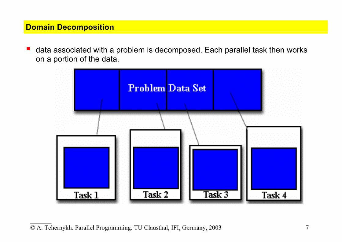
Domain Decomposition data associated with a problem is decomposed. Each parallel task then works

on a portion of the data.

____________


Data partition

____________


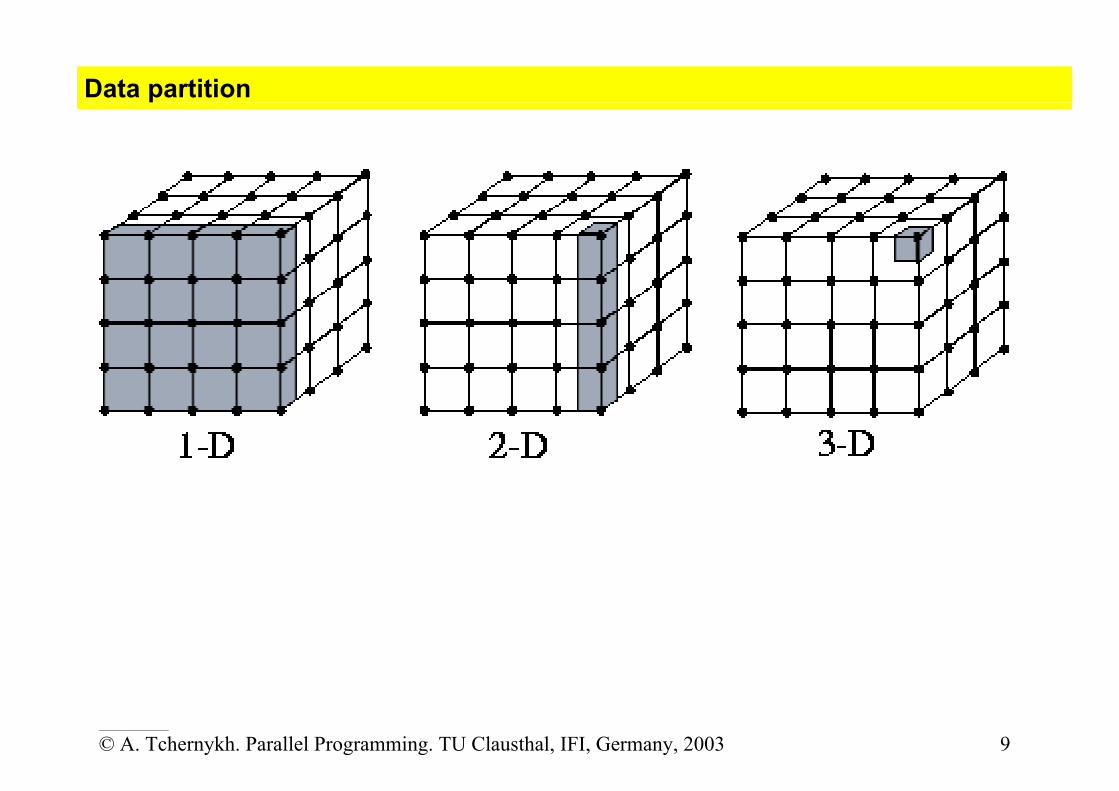
Data partition

Some standard domain decompositions of a regular 2D grid (array) include: BLOCK: contiguous chunks of rows or columns of data on each processor. BLOCK-BLOCK: block decomposition in both dimensions. CYCLIC: data is assigned to processors like cards dealt to poker players, so

neighbouring points are on different processors. This can be good for load balancing applications with varying workloads that have certain types of communication, e.g. very little, or a lot (global sums or all-to-all), or strided. BLOCK-CYCLIC: a block decomposition in one dimension, cyclic in the other. SCATTERED: points are scattered randomly across processors. This can be good for

load balancing applications with little (or lots of) communication. The human brain seems to work this way { neighboring sections may control widely separated parts of the body.

Basic idea: Each array element can be re-computed independently of all others. Huge degree of concurrency, usually exceeds available processing elements. Combine individual elements to groups. Associate each group with one processing element.

____________


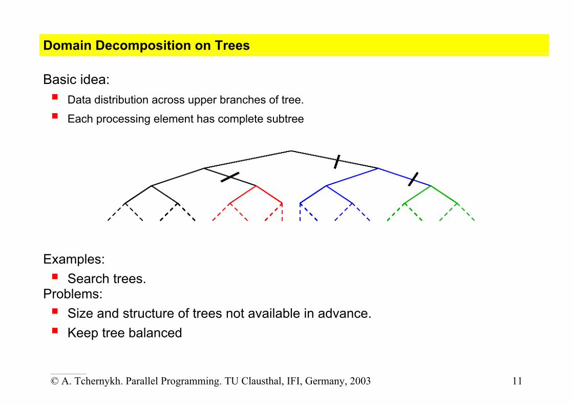
Domain Decomposition on Trees Basic idea: Data distribution across upper branches of tree. Each processing element has complete subtree

Examples: Search trees.

Problems: Size and structure of trees not available in advance. Keep tree balanced

____________


Domain Decomposition on Irregular Meshes Basic idea: Irregular distribution of points.

Each point has some maximum number of neighbours.

New points may be introduced. ____ _

Problems: Very irregular data structure.

Difficult to keep balanced among processing elements.

Difficult to find good distributions,

____________


Functional Decomposition The focus is on the computation that is to be performed rather than on the data

manipulated by the computation. The problem is decomposed according to the work that must be done. Each task performs a portion of the overall work.

____________


Functional Decomposition

• Good for problems that can be split into different tasks. • For example: Climate Modeling

o Each model component can be thought of as a separate task. o They can exchange data between components during computation:

atmosphere model generates wind velocity data that are used by the ocean model

ocean model generates sea surface temperature data that are used by the atmosphere model

and so on.

• Combining these two types of problem decomposition is common and natural.

____________


Decomposition method: Dynamic Unfolding

Characteristics: Task is either solved sequentially or is recursively split into subtasks. Subtasks are computed in parallel. Task waits for subtasks to ¯nish. Task combines partial results of

subtasks. Examples: Quick Sort. All divide-and-conquer algorithms. Combinatorial optimization. Integer optimization.

____________


Partitioning Design Checklist The partitioning phase should produce one or more possible decompositions of a problem. Before proceeding to evaluate communication requirements, ensure that the design has no obvious flaws.

Generally, all these questions should be answered in the affirmative. Does your partition define at least an order of magnitude more tasks than there

are processors in your target computer? If not, you have little flexibility in subsequent design stages. Does your partition avoid redundant computation and storage requirements? If

not, the resulting algorithm may not be scalable to deal with large problems. Are tasks of comparable size? If not, it may be hard to allocate each processor

equal amounts of work. Does the number of tasks scale with problem size? Ideally, an increase in

problem size should increase the number of tasks rather than the size of individual tasks. If this is not the case, your parallel algorithm may not be able to solve larger problems when more processors are available.

____________


Partitioning Design Checklist Have you identified several alternative partitions? You can maximize flexibility

in subsequent design stages by considering alternatives now. Remember to investigate both domain and functional decompositions.

Negative answers to these questions may suggest that, we have a ``bad'' design. In this situation risky simply to push ahead with implementation. use the performance evaluation techniques to determine whether the design

meets our performance goals despite its apparent deficiencies. revisit the problem specification. Particularly in science and engineering

applications, where the problem to be solved may involve a simulation of a complex physical process, the approximations and numerical techniques used to develop the simulation can strongly influence the ease of parallel implementation. In some cases, optimal sequential and parallel solutions to the same problem

may use quite different solution techniques.

____________


Communication

____________


Communication The tasks generated by a partition are intended to execute concurrently but cannot, in general, execute independently. Communication patterns are categorize along four loosely orthogonal axes: local/global, structured/unstructured, static/dynamic, synchronous/asynchronous.

In local communication, each task communicates with a small set of other tasks (its ``neighbors'');

____________


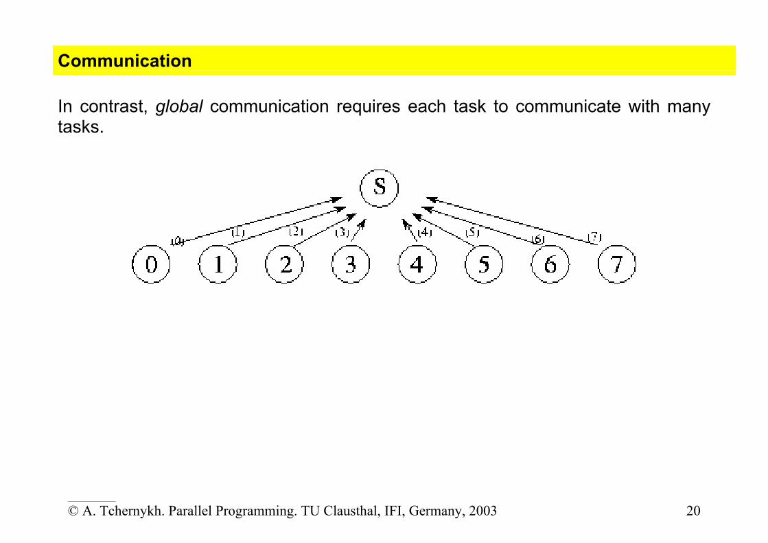
Communication In contrast, global communication requires each task to communicate with many tasks.

____________


Communication In structured communication, a task and its neighbors form a regular structure,

such as a tree or grid; in contrast, unstructured communication networks may be arbitrary graphs.

____________


Communication In static communication, the identity of communication partners does not

change over time; in contrast, the identity of communication partners in dynamic communication

structures may be determined by data computed at runtime and may be highly variable.

In synchronous communication, producers and consumers execute in a

coordinated fashion, with producer/consumer pairs cooperating in data transfer operations;

in contrast, asynchronous communication may require that a consumer obtain

data without the cooperation of the producer.

____________


Communication Design Checklist

1. Do all tasks perform about the same number of communication operations? Unbalanced communication requirements suggest a nonscalable construct. Revisit your design to see whether communication operations can be distributed more equitably. For example, if a frequently accessed data structure is encapsulated in a single task, consider distributing or replicating this data structure.

2. Does each task communicate only with a small number of neighbors? If each task must communicate with many other tasks, evaluate the possibility of formulating this global communication in terms of a local communication structure.

3. Are communication operations able to proceed concurrently? If not, your algorithm is likely to be inefficient and nonscalable. Try to use divide-and-conquer techniques to uncover concurrency.

4. Is the computation associated with different tasks able to proceed concurrently?

If not, your algorithm is likely to be inefficient and nonscalable. Consider whether you can reorder communication and computation operations. You may also wish to revisit your problem specification.

____________


Agglomeration

____________


Agglomeration In the third stage of the agglomeration we revise decisions made in the partitioning and communication phases

with a view to obtaining an algorithm that will execute efficiently on some class of parallel computer.

• consider whether it is useful to combine, or agglomerate, tasks identified by the partitioning phase, so as to provide a smaller number of tasks, each of greater size.

• determine whether it is worthwhile to replicate data and/or computation.

____________


Agglomeration

____________


Agglomeration The number of tasks may be greater than the number of processors. In this case, our design remains somewhat abstract, since issues relating to the mapping of tasks to processors remain unresolved. during the agglomeration phase we have to reduce the number of tasks to

exactly one per processor. address the mapping problem. increase task granularity.

3 (conflicting) goals guide decisions concerning agglomeration and replication: reducing communication costs by increasing computation and communication

granularity, retaining flexibility with respect to scalability and mapping decisions, reducing software engineering costs.

____________


Agglomeration. Increasing Granularity

____________


Agglomeration If the number of communication partners per task is small, we can often reduce both the number of communication operations and the total communication volume by increasing the granularity of our partition, that is, by agglomerating several tasks into one. communication requirements of a task are proportional to the

o surface of the subdomain on which it operates, o subdomain's volume.

In a two-dimensional problem,

o ̀`surface'' scales with the problem size while o ̀`volume'' scales as the problem size squared.

Hence, the amount of communication performed for a unit of computation (the communication/computation ratio ) decreases as task size increases. This effect is often visible when a partition is obtained by using domain

decomposition techniques.

____________


Agglomeration Design Checklist

1. Has agglomeration reduced communication costs by increasing locality?

If not, examine your algorithm to determine whether this could be achieved using an alternative agglomeration strategy.

2. If agglomeration has replicated computation, have you verified that the benefits of this replication outweigh its costs, for a range of problem sizes and processor counts?

3. If agglomeration replicates data, have you verified that this does not compromise the scalability of your algorithm by restricting the range of problem sizes or processor counts?

4. Has agglomeration yielded tasks with similar computation and communication costs?

The larger the tasks created by agglomeration, the more important it is that they have similar costs. If we have created just one task per processor, then these tasks should have nearly identical costs.

5. Does the number of tasks still scale with problem size? If not, then your algorithm is no longer able to solve larger problems on larger parallel computers.

____________


Agglomeration Design Checklist

6. If agglomeration eliminated opportunities for concurrent execution, have you verified that there is sufficient concurrency for current and future target computers?

An algorithm with insufficient concurrency may still be the most efficient, if other algorithms have excessive communication costs; performance models can be used to quantify these tradeoffs.

7. Can the number of tasks be reduced still further, without introducing load imbalances, increasing software engineering costs, or reducing scalability?

algorithms that create fewer larger-grained tasks are often simpler and more efficient than those that create many fine-grained tasks.

8. If you are parallelizing an existing sequential program, have you considered the cost of the modifications required to the sequential code?

If these costs are high, consider alternative agglomeration strategies that increase opportunities for code reuse. If the resulting algorithms are less efficient, use performance modeling techniques to estimate cost tradeoffs.

____________


Mapping

____________


Mapping The mapping problem does not arise on uniprocessors or on shared-memory computers that provide automatic task scheduling.

In these computers, a set of tasks and associated communication requirements is a sufficient for a parallel algorithm; operating system or hardware mechanisms can be relied upon to schedule

executable tasks to available processors. General-purpose mapping mechanisms have yet to be developed for scalable parallel computers. Mapping remains a difficult problem that must be explicitly addressed when designing parallel algorithms. The goal in developing mapping algorithms is to minimize total execution time. Two strategies are to achieve this goal:

1. tasks that are able to execute concurrently are placed on different processors, so as to enhance concurrency.

2. tasks that communicate frequently are placed on the same processor, so as to increase locality.

____________


Mapping

These two strategies will sometimes conflict, in which case the design will involve tradeoffs.

Resource limitations may restrict the number of tasks that can be placed on a single processor. The mapping problem is known to be NP -complete, meaning that no computationally tractable (polynomial-time) algorithm can exist for evaluating these tradeoffs in the general case. specialized strategies and heuristics

are applied

____________


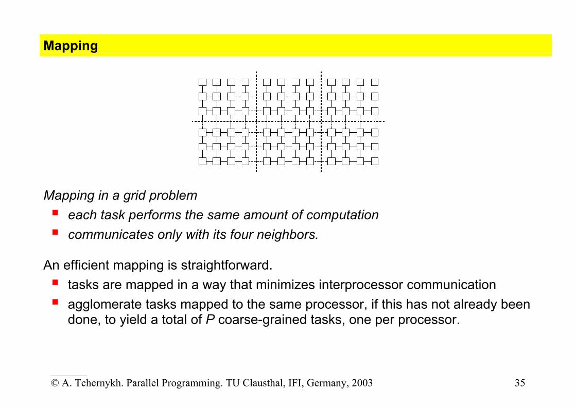
Mapping

Mapping in a grid problem each task performs the same amount of computation communicates only with its four neighbors.

An efficient mapping is straightforward. tasks are mapped in a way that minimizes interprocessor communication agglomerate tasks mapped to the same processor, if this has not already been

done, to yield a total of P coarse-grained tasks, one per processor.

____________


Mapping In more complex domain decomposition-based algorithms with variable

amounts of work per task and/or unstructured communication patterns, efficient agglomeration and mapping strategies may not be obvious to the programmer.

Hence, load balancing algorithms that seek to identify efficient agglomeration

and mapping strategies, typically by using heuristic techniques are employed. The most complex problems are those in which either the number of tasks or

the amount of computation or communication per task changes dynamically during program execution. In the case of problems developed using domain decomposition techniques,

we may use a dynamic load-balancing strategy in which a load-balancing algorithm is executed periodically to determine a new agglomeration and mapping.

____________


Load Balancing

____________


Load Balancing distributing work among tasks so that

o all tasks are kept busy all of the time. o minimization of idle time.

important for performance reasons. if tasks are synchronized, the slowest task will determine the overall

performance.

____________


Static Load Balancing

For maximum efficiency, domain decomposition should give equal work to each processor. In building the wall, can just give each bricklayer an equal length segment.

But things can become much more complicated: • What if some bricklayers are faster than others? (this is like an

inhomogeneous cluster of different workstations) • What if there are guard towers every few hundred meters, which require more

work to construct? (in some applications, more work is required in certain parts of the domain)

If we know in advance 1. the relative speed of the processors, and 2. the relative amount of processing required for each part of the problem

then we can do a domain decomposition that takes this into account, so that different processors may have different sized domains, but the time to process them will be about the same. This is static load balancing, and can be done at compile-time.

For some applications, maintaining load balance while simultaneously minimizing communication can be a very difficult optimization problem.

____________


Dynamic Load Balancing

In some cases we do not know in advance one (or both) of: effective performance of the processors { may be sharing the processors with

other applications, so the load and available CPU may vary) amount of work required for each part of the domain { many applications are

adaptive or dynamic, and the workload is only known at runtime} In this case we need to dynamically change the domain decomposition by

periodically repartitioning the data between processors. This is dynamic load balancing, and it can involve substantial overheads in: Figuring out how to best repartition the data { may need to use a fast method

that gives a good (but not optimal) domain decomposition, to reduce computation. Moving the data between processors { could restrict this to local (neighbouring

processor) moves to reduce communication. Usually repartition as infrequently as possible (e.g. every few iterations instead of

every iteration). There is a tradeoff between performance improvement and repartitioning overhead.

____________


How to Achieve Load Balance Equally partition the work each task receives For array/matrix operations where each task performs similar work, evenly

distribute the data set among the tasks. For loop iterations where the work done in each iteration is similar, evenly

distribute the iterations across the tasks. If a heterogeneous mix of machines with varying performance characteristics

are being used, be sure to use some type of performance analysis tool to detect any load imbalances. Adjust work accordingly.

____________


How to Achieve Load Balance

Dynamic work assignment Certain classes of problems result in load imbalances even if data is evenly

distributed among tasks: o Sparse arrays - some tasks will have actual data to work on while others

have mostly "zeros". o Adaptive grid methods - some tasks may need to refine their mesh while

others don't. When the amount of work each task will perform is intentionally variable, or

is unable to be predicted, it may be helpful to use a scheduler - task pool approach. As each task finishes its work, it queues to get a new piece of work. It become necessary to design an algorithm which detects and handles load

imbalances as they occur dynamically within the code.

____________


Common Task Pool approach

____________


Loop Scheduling Types

____________


Loop Scheduling Types

simple partition the iterations evenly among all the available threads.

dynamic gives each thread chunksize iterations. Chunksize should be smaller than the number of total iterations divided by

the number of threads. The advantage of dynamic over simple is that dynamic helps distribute the work more evenly than simple.

interleave gives each thread chunksize iterations of the loop, which are then assigned to

the threads in an interleaved way. gss (guided self-scheduling)

gives each processor a varied number of iterations of the loop. This is like dynamic, but instead of a fixed chunksize, the chunksize iterations begin with big pieces and end with small pieces.

Programs with triangular matrices should use gss. runtime

Tells the compiler that the real schedule type will be specified at run time.

____________


Load balancing. MPMD – Multiple Program, Multiple Data

Characteristics: Constant number of tasks. Each task may execute different program. Tasks operate on pairwise disjoint data sets.

____________


Load balancing. SPMD – Single Program, Multiple Data

Characteristics: Constant number of tasks. Each task executes identical program. Tasks operate on pairwise disjoint data sets. Tasks may identify themselves !

____________


Dynamic Task Creation Changing number of tasks.

A

B C

D E

Parent process

Child processes

Can extend any of the previous organization principles: MPMD SPMD Master - Worker

____________


Load balancing. Master – Worker balancing structure

A central manager task is given responsibility for problem allocation. Each worker repeatedly requests and executes a problem from the manager. Workers can also send new tasks to the manager for allocation to other

workers. The efficiency of this strategy depends on the number of workers and the

relative costs of obtaining and executing problems. Efficiency can be improved by prefetching problems so as to overlap computation and communication, caching problems in workers, so that workers communicate with the manager

only when no problems are available locally.

____________


Load balancing. Master – Worker balancing structure Hierarchical Manager/Worker. A variant of the manager/worker scheme divides workers into disjoint sets, each with a submanager. Workers request tasks from submanagers, which themselves communicate periodically with the manager and with other submanagers to balance load between the sets of processors for which they are responsible. Decentralized Schemes. there is no central manager. a separate task pool is maintained on each processor, and idle workers request problems from other processors. task pool becomes a distributed data structure that is accessed by the different tasks in an asynchronous fashion. A variety of access policies can be defined. a worker may request work from a small number of predefined “neighbors” may select other processors at random.

____________


Load balancing. Master – Worker balancing structure In a hybrid centralized/distributed scheme, requests are sent to a central manager, which allocates them to workers in a round-robin fashion. Notice that while this manager will certainly be a bottleneck on large numbers of processors, it will typically be accessed less frequently than will the manager in a manager/worker scheduler and hence is a more scalable construct. access to a distributed data structure, such as the task pool maintained by a

decentralized load-balancing scheme, can be provided in several different ways. o Workers can be made responsible for both computing and managing the

queue of problems. each worker must periodically poll to detect pending requests.

o Alternatively, computation and task pool management responsibilities can be encapsulated in separate tasks.

____________


Mapping Design Checklist mapping decisions seek to balance conflicting requirements for equitable load

distribution and low communication costs. static mapping scheme allocates each task to a single processor when the number or size of tasks is variable or not known until runtime, we

may use a dynamic load balancing scheme or reformulate the problem so that a task scheduling structure can be used to schedule computation.

The following checklist can serve as a basis for an informal evaluation of the mapping design.

1. If considering an SPMD design for a complex problem, have you also considered an algorithm based on dynamic task creation and deletion?

The latter approach can yield a simpler algorithm; however, performance can be problematic.

____________


Mapping Design Checklist

2. If considering a design based on dynamic task creation and deletion, have you also considered an SPMD algorithm?

An SPMD algorithm provides greater control over the scheduling of communication and computation, but can be more complex.

3. If using a centralized load-balancing scheme, have you verified that the manager will not become a bottleneck?

You may be able to reduce communication costs in these schemes by passing pointers to tasks, rather than the tasks themselves, to the manager.

4. If using a dynamic load-balancing scheme, have you evaluated the relative costs of different strategies?

Be sure to include the implementation costs in your analysis.

____________


Parallel Program Examples

____________


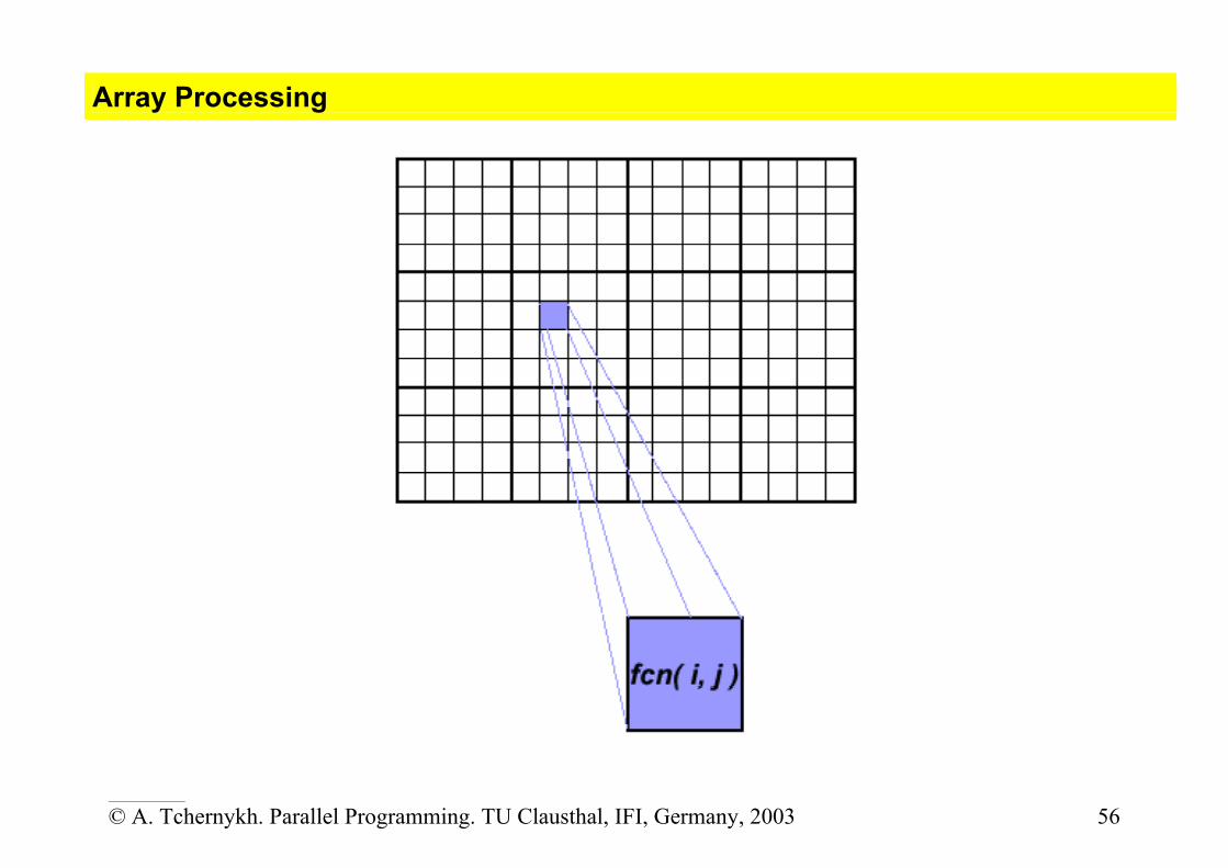
Array Processing

• This example demonstrates calculations on 2-dimensional array elements, with the computation on each array element being independent from other array elements.

• The serial program calculates one element at a time in sequential order. • Serial code could be of the form:

do j = 1,n do i = 1,n a(i,j) = fcn(i,j) end do end do

• The calculation of elements is independent of one another - leads to an

embarrassingly parallel situation. • The problem should be computationally intensive.

____________


Array Processing

____________


Array Processing. Parallel Solution 1 Arrays elements are distributed so that each processor owns a portion of an

array (subarray). Independent calculation of array elements insures there is no need for

communication between tasks. Distribution scheme is chosen by other criteria, e.g. unit stride (stride of 1)

through the subarrays. Unit stride maximizes cache/memory usage. Since it is desirable to have unit stride through the subarrays, the choice of a

distribution scheme depends on the programming language. After the array is distributed, each task executes the portion of the loop

corresponding to the data it owns. For example, with Fortran block distribution: do j = mystart, myenddo i = 1,n a(i,j) = fcn(i,j) end do end do

• Notice that only the outer loop variables are different from the serial solution.

____________


Array Processing. Parallel Solution Implementation

• Implement as SPMD model. • Master process initializes array, sends info to worker processes and receives

results. • Worker process receives info, performs its share of computation and sends

results to master. • perform block distribution of the array.

____________


Array Processing. Parallel Solution Implementation Pseudo code solution: red highlights changes for parallelism.

find out if I am MASTER or WORKER if I am MASTER initialize the array send each WORKER info on part of array it owns send each WORKER its portion of initial array receive from each WORKER results else if I am WORKER receive from MASTER info on part of array I own receive from MASTER my portion of initial array # calculate my portion of array do j = my first column, my last column do i = 1,n a(i,j) = fcn(i,j) end do end do send MASTER results endif

____________


Array Processing. Parallel Solution 2. Pool of Tasks

The previous array solution demonstrated static load balancing: Each task has a fixed amount of work to do May be significant idle time for faster or more lightly loaded processors -

slowest tasks determines overall performance. Static load balancing is not usually a major concern if all tasks are performing the same amount of work on identical machines. If you have a load balance problem (some tasks work faster than others), you may benefit by using a "pool of tasks" scheme.

____________


Array Processing. Parallel Solution 2. Pool of Tasks Pool of Tasks Scheme:

• Two processes are employed Master Process:

o Holds pool of tasks for worker processes to do o Sends worker a task when requested o Collects results from workers

Worker Process: repeatedly does the following o Gets task from master process o Performs computation o Sends results to master

• Worker processes do not know before runtime which portion of array they will handle or how many tasks they will perform.

• Dynamic load balancing occurs at run time: the faster tasks will get more work to do.

____________


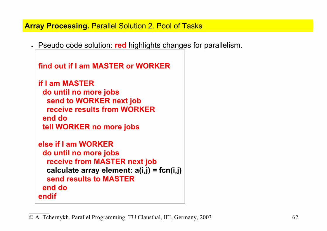
Array Processing. Parallel Solution 2. Pool of Tasks

• Pseudo code solution: red highlights changes for parallelism. find out if I am MASTER or WORKER if I am MASTER do until no more jobs send to WORKER next job receive results from WORKER end do tell WORKER no more jobs else if I am WORKER do until no more jobs receive from MASTER next job calculate array element: a(i,j) = fcn(i,j) send results to MASTER end do endif

____________


Array Processing. Parallel Solution 2. Pool of Tasks Discussion: In the above pool of tasks example, each task calculated an individual array

element as a job. The computation to communication ratio is finely granular. Finely granular solutions incur more communication overhead in order to

reduce task idle time. A more optimal solution might be to distribute more work with each job. The

"right" amount of work is problem dependent.

____________


Matrix Vector Multiplication.

We will develop a parallel application for multiplying a matrix A of m rows

and n columns times a vector b of n elements to produce a vector c of m elements. Note that the multiplication c=A*b can be performed two ways

o The first way [ called the DOTPRODUCT or (i,j) method ] is to compute each element of the result output vector as a inner product of a row vector of the input matrix A to the vector b.

o The second method [ called the SAXPY or (j,i) method ] proceeds as follows. The algorithm proceeds by computing the scalar product of each element of the b vector with a column vector of the A matrix and summing up the intermediate result vectors to form the output vector.

We will use the second method for our parallel implementation.

____________


Matrix Vector Multiplication.

____________


Matrix Vector Multiplication. /* serial matrix vector multiplication program */ matvec() { int i,j; for (j=0; j < n; j++) { for (i=0; i < m; i++) { c[ i ] = c[ i ] + a[ i ][ j ] * b[ j ]; } } }

____________


Matrix Vector Multiplication. Shared Memory Parallel Implementation Shared Memory Parallel Algorithm

We will partition the problem by allowing each processor to perform the

multiplication of a set of columns of the input matrix times the corresponding sets of elements of the input vector to produce an intermediate result vector. The computations of each intermediate vector will be performed in parallel

among all the processors. These intermediate vectors are going to be accumulated among the

processors in a sequential step. We will use a static interleaved scheduling algorithm for distributing the j

index iterations of the matrix vector multiplication loop. A processor i picks the iterations i, i+p, i+2p, and so on, where p is the

number of processors, determined at runtime.

____________


Matrix Vector Multiplication. Shared Memory Parallel Implementation m_set_procs(nproc); /* create nprocs parallel threads */ m_fork(matvec); /* perform parallel multiplication */ m_sync(); /* wait for all threads to complete */ void matvec() { int i,j,nprocs,myid; float tmp[max]; nprocs = m_get_numprocs(); myid = m_get_myid(); for (j = myid; j < n; j = j + nprocs) { for (i=0; i < m; i++) tmp[i] = tmp[i] + a[i][j] * b[j]; m_lock(); for (i=0; i < m; i++) c[i] = c[i] + tmp[i]; m_unlock(); } }

____________


Matrix Multiplication There are many ways of performing matrix multiplication, which multiplies

matrices a and b of sizes n*n and produces a result matrix c. We show one way in the following program Each result matrix element is obtained as an inner product of a row of the a

matrix (containing n elements) times a column of the b matrix (containing n elements). The program first reads the value of the size of the matrices, then reads the

data for the two matrices, an then performs the matrix computation and prints out the results.

____________


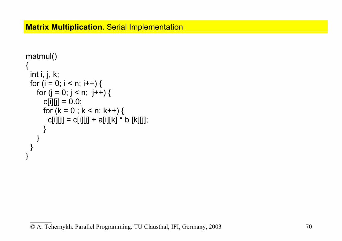
Matrix Multiplication. Serial Implementation matmul() { int i, j, k; for (i = 0; i < n; i++) { for (j = 0; j < n; j++) { c[i][j] = 0.0; for (k = 0 ; k < n; k++) { c[i][j] = c[i][j] + a[i][k] * b [k][j]; } } } }

____________


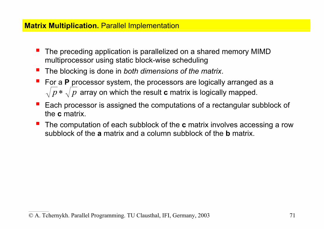
Matrix Multiplication. Parallel Implementation

The preceding application is parallelized on a shared memory MIMD multiprocessor using static block-wise scheduling The blocking is done in both dimensions of the matrix. For a P processor system, the processors are logically arranged as a

pp ∗ array on which the result c matrix is logically mapped.

Each processor is assigned the computations of a rectangular subblock of the c matrix. The computation of each subblock of the c matrix involves accessing a row

subblock of the a matrix and a column subblock of the b matrix.

____________


Matrix Multiplication. Parallel Implementation m_set_procs(nprocs); /* set number of processes */ m_fork(matmul); /* execute parallel loop */ m_kill_procs(); /* kill child processes */

void matmul() { int i, j, k; int nprocs, iprocs, jprocs; int my_id, i_id,j_id,ilb,iub,jlb,jub; nprocs = m_get_numprocs(); /* number of processors */ iprocs = (int) sqrt((double) nprocs); /* number of processors in i direction */ jprocs = nprocs / iprocs; /* number of processors in j direction */

____________


Matrix Multiplication. Parallel Implementation my_id = m_get_myid(); i_id = my_id % iprocs; /* get processor ID in i and j dimensions */ j_id = my_id % jprocs; ilb = i_id * n / iprocs; /* find lower and upper bounds of i loop */ iub = (i_id + 1) * (n / iprocs); jlb = j_id * n / jprocs; /* find lower and upper bounds of j loop */ jub = (j_id + 1) * (n / jprocs);

for (i = ilb; i < iub; i++) for (j = jlb; j < jub; j++) { c[i][j] = 0.0; for (k = 0 ; k < n; k++) c[i][j] = c[i][j] + a[i][k] * b [k][j]; } }

____________


Quick Sort

• Quicksort is one of the most common sorting algorithms whose average complexity is O(n log (n).

• It is a divide and conquer algorithm that sorts sequences by recursively dividing into smaller sequences

• Let the sequence be A[1...n] • two steps:

o During the divide step, a sequence A[q..r] is partitioned into two nonempty subsequences A[q..s] and A[s+1..r] such that each element of A[q..s] <= each element of A[s+1..r]

o During conquer step, the subsequent subsequences are sorted by recursively applying quicksort.

• Partitioning - select a pivot x randomly between q and r

____________


Quick Sort. Serial Algorithm QUICKSORT(A,q,r)

begin if q<r then x=A[q]; s=q; for i=q+1 to r if A[i]<=x then s=s+1; swap(A[s],A[i]); end if end i-loop swap(A[q],A[s]); QUICKSORT(A,q,s); QUICKSORT(A,s+1,r); end if end QUICKSORT

QSORT(start,end) { if (start==end) return; x=a[start]; i=start-1; j=end+1; while (i<j) { j--; while ((a[ j ]>x)&&(j>start)) j--; i++; while ((x>a[ i ])&&(i<end)) i++; if (i<j) { temp=a[ i ]; a[ i ]=a[ j ]; a[ j ]=temp; } } qsort(start,j); qsort(j+1,end); } main() { qsort(0,N-1); }

____________


Quick Sort. Parallel Implementation

• during each call to QUICKSORT array is partitioned into two parts. • Each of two parts can be solved independently

#include <stdio.h> #include <stdlib.h> #define N 100 int a[N]; int start[N],end[N]; int head,tail,numdone; int pivot(start,end) int start,end; { int x,i,j,temp;

____________



if (start==end) return(start); x=a[start]; i=start-1; j=end+1; while (i<j) { j--; while ((a[j]>x)&&(j>start)) j--; i++; while ((x>a[i])&&(i<end)) i++; if (i<j) { temp=a[i]; a[i]=a[j]; a[j]=temp; } } return(j); }

____________



parallel_qsort() { int l_start, l_end, l_pivot, l_flag, l_numdone, id; id=m_get_myid(); l_numdone=0; while (l_numdone<N) { l_flag=0; m_lock(); if (head<tail) { l_flag=1; l_start=start[head]; l_end=end[head]; head++; printf("[%d] : (%d,%d)\n",id,l_start,l_end); } l_numdone=numdone; m_unlock();

____________



if (l_flag==1) { l_pivot=pivot(l_start,l_end); m_lock(); if (l_start<l_pivot) { start[tail]=l_start; end[tail]=l_pivot; tail++; } else { numdone++; } if (l_pivot+1<l_end) { start[tail]=l_pivot+1; end[tail]=l_end; tail++; } else { numdone++; } l_numdone=numdone; m_unlock();

____________



} } } main() { int i; for (i=0;i<N;i++) a[i]=rand()%N; head=0; tail=1; start[0]=0; end[0]=N-1; m_set_procs(4); m_fork(parallel_qsort); m_kill_procs(); for (i=0;i<N;i++) printf("%d ",a[i]); printf("\n"); }

____________


Parallel Program Examples. PI Calculation Problem

• Consider parallel algorithm for computing the value of through the following numerical integration

dxx

Pi ∫ +=

1

021

4

This integration can be evaluated by computing the area under the curve for

214)(x

xf+

= from 0 to 1.

• With numerical integration using the rectangle rule for decomposition, one divides the region x from 0 to 1 into n points.

• The value of the function is evaluated at the midpoint of each interval • The values are summed up and multiplied by the width of one interval.

____________


Parallel Program Examples. PI Calculation

____________


Pi: Sequential Algorithm pi() { h = 1.0 / n; sum = 0.0; for (i=0; i < n; i++) { x = h * (i - 0.5); sum = sum + 4.0 / (1 + x * x); } pi = h * sum; }

____________


Pi: Sequential Algorithm #include <stdio.h> #include <stdlib.h> double piece_of_pi(int); main(int argc, char *argv[]){ double y; double total_pi; int n; n = atoi(argv[1]); y = piece_of_pi(nrects); printf("Pi=: %15.13f\n\n",y); return(0); } double piece_of_pi(int nrects){ double x, width, total_pi; int i; width = 1.0/n; for(i=0;i<n; i++){ x = (i+0.5)*width; total_pi += 4.0/(1+x*x); } total_pi*= width; return(total_pi); }

____________


Pi: Parallel Algorithm

• Each processor computes on a set of about points which are allocated to each processor in a cyclic manner

• Finally, we assume that the local values of are accumulated among the p processors under synchronization

____________


Pi: Parallel Program 1. Shared Memory Parallel Implementation #include <stdio.h> int main() { long n=30000000,i; long double h=0, pi=0, x, sum; h=1.0/(long double)n; #pragma parallel shared(pi) byvalue(h) local(x,i,sum) { sum=0; x=0; #pragma pfor for(i=0;i<n; i++) { x = ( i + 0.5 )*h; sum += ( 4.0 / ( 1.0 + x * x )) * h; } #pragma critical pi+=suma; } printf("Pi =: %16.14Lf \n", pi); return 0; }

____________


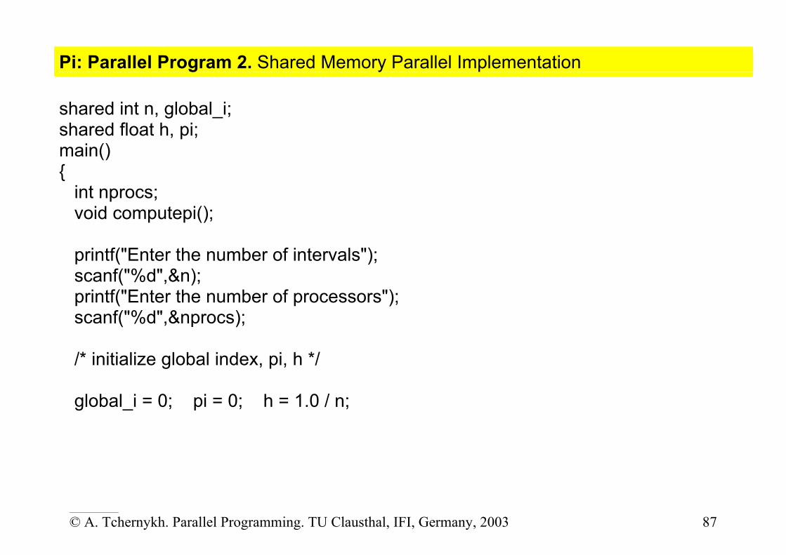
Pi: Parallel Program 2. Shared Memory Parallel Implementation shared int n, global_i; shared float h, pi; main() { int nprocs; void computepi(); printf("Enter the number of intervals"); scanf("%d",&n); printf("Enter the number of processors"); scanf("%d",&nprocs); /* initialize global index, pi, h */ global_i = 0; pi = 0; h = 1.0 / n;

____________


Pi: Parallel Program 2. Shared Memory Parallel Implementation /* create nprocs parallel threads */ m_set_procs(nprocs); /* compute pi in parallel */ m_fork(computepi); /* wait for all threads to complete */ m_sync(); printf("Value of pi is %f",pi); }

____________


Pi: Parallel Program 2. Shared Memory Parallel Implementation void computepi() { int i; float sum, localpi, x; sum = 0.0; while (i < n) { m_lock(); i = global_i; global_i = global_i + 1; m_unlock(); x = h * (i - 0.5); sum = sum + 4.0 / (1 + x * x); } localpi = h * sum; m_lock(); pi = pi + localpi; m_unlock(); }

____________


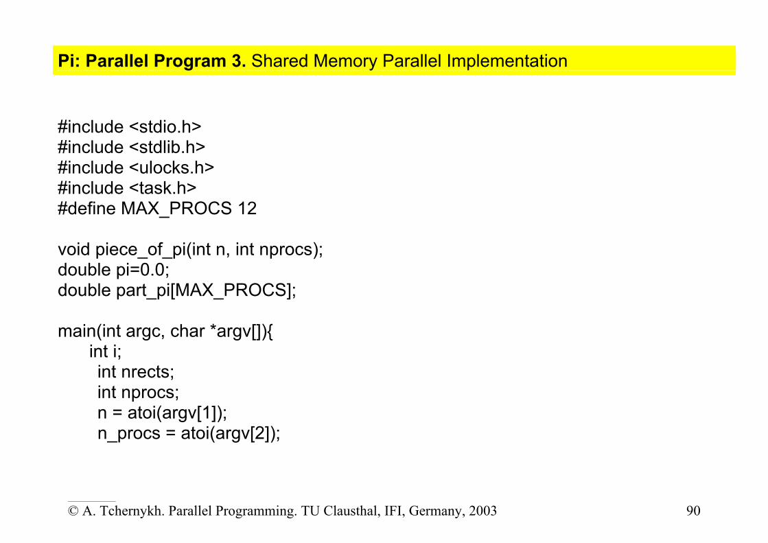
Pi: Parallel Program 3. Shared Memory Parallel Implementation #include <stdio.h> #include <stdlib.h> #include <ulocks.h> #include <task.h> #define MAX_PROCS 12 void piece_of_pi(int n, int nprocs); double pi=0.0; double part_pi[MAX_PROCS]; main(int argc, char *argv[]){ int i; int nrects; int nprocs; n = atoi(argv[1]); n_procs = atoi(argv[2]);

____________


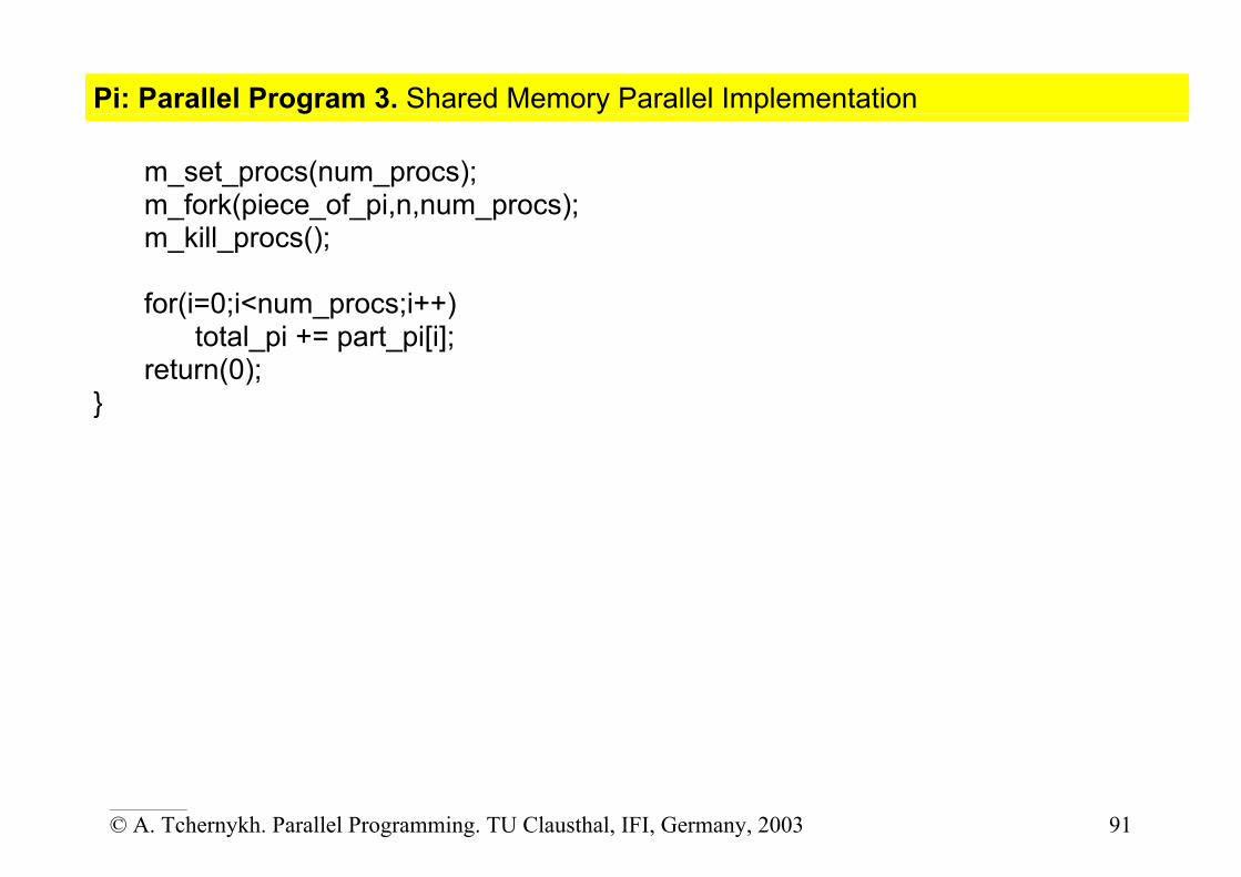
Pi: Parallel Program 3. Shared Memory Parallel Implementation m_set_procs(num_procs); m_fork(piece_of_pi,n,num_procs); m_kill_procs(); for(i=0;i<num_procs;i++) total_pi += part_pi[i]; return(0); }

____________


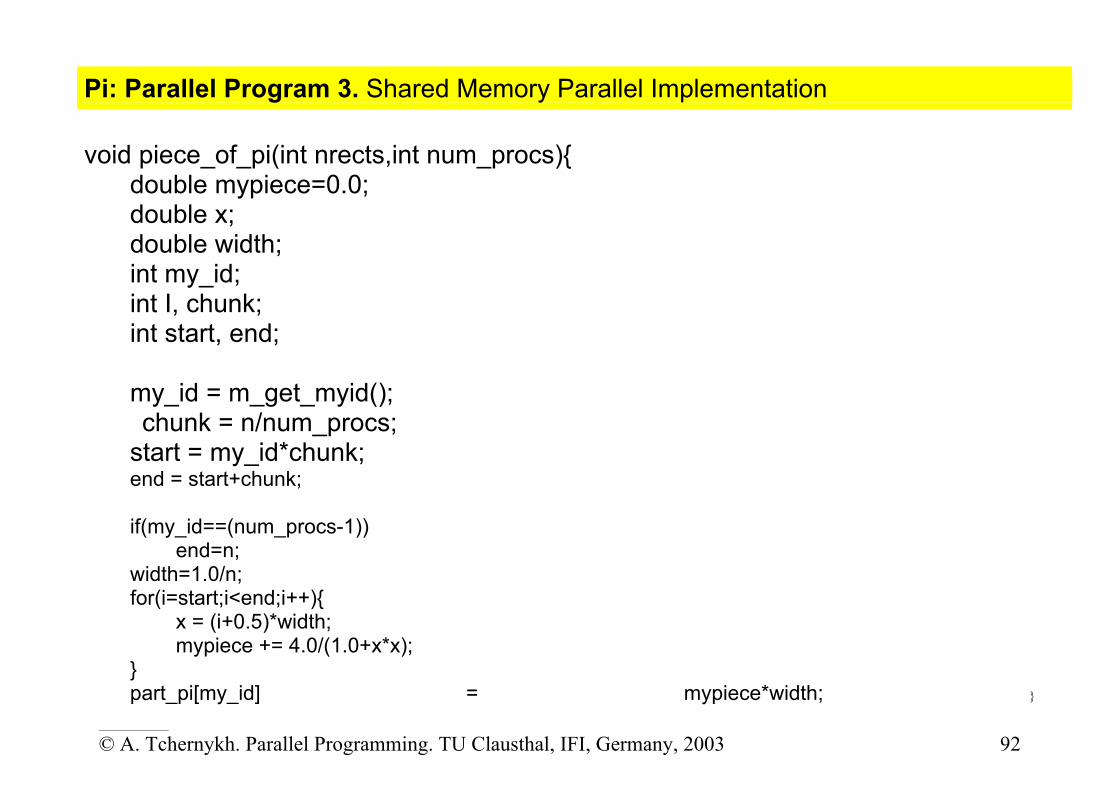
Pi: Parallel Program 3. Shared Memory Parallel Implementation void piece_of_pi(int nrects,int num_procs){ double mypiece=0.0; double x; double width; int my_id; int I, chunk; int start, end; my_id = m_get_myid(); chunk = n/num_procs; start = my_id*chunk; end = start+chunk; if(my_id==(num_procs-1)) end=n; width=1.0/n; for(i=start;i<end;i++){ x = (i+0.5)*width; mypiece += 4.0/(1.0+x*x); } part_pi[my_id] = mypiece*width; }

____________


Pi: Solution 3.

____________


Pi: Solution 3.

• The value of PI can be calculated in a number of ways. Consider the following method of approximating PI

1. Inscribe a circle in a square 2. Randomly generate points in the square 3. Determine the number of points in the square that are also in the circle 4. Let r be the number of points in the circle divided by the number of points

in the square 5. PI ~ 4 r 6. Note that the more points generated, the better the approximation

____________


Pi: Solution 3.

• Serial pseudo code for this procedure: npoints := 10000 ; circle_count := 0 ; for i := 1 to npoints xcoordinate := random( 0,1) ; ycoordinate := random( 0,1) ; if (xcoordinate, ycoordinate) inside circle then circle_count := circle_count + 1 ; endif endfor PI = 4.0 * circle_count/npoints ;

• Note that most of the time in running this program would be spent executing the loop

• Leads to an embarrassingly parallel solution o Computationally intensive o Minimal communication, Minimal I/O

____________


Pi: Parallel Solution 3.

• Parallel strategy: break the loop into portions that can be executed by the tasks.

• For the task of approximating PI: o Each task executes its portion of the loop a number of times. o Each task can do its work without requiring any information from the other

tasks (there are no data dependencies). o Uses the SPMD model. One task acts as master and collects the results.

____________



• pseudo code solution: red highlights changes for parallelism. npoints = 10000 circle_count = 0 p = number of tasks num = npoints/p for i := 1 to num generate 2 random numbers between 0 and 1 xcoordinate = random1 ; ycoordinate = random2 if (xcoordinate, ycoordinate) inside circle then circle_count = circle_count + 1 endif endfor find out if I am MASTER or WORKER if I am MASTER % task_id() = 0 receive from WORKERS their circle_counts compute PI (use MASTER and WORKER calculations)

____________



for i := 1 to num_tasks() - 1 tmp := receive( i) ; circle_count := circle_count + tmp ; endfor PI = 4.0 * circle_count/npoints ; else if I am WORKER % task_id() > 0send to MASTER circle_count endif

____________


Notes

These materials were developed in part from the following sources Livermore Computing Training Materials available on WEB

http://www.llnl.gov/computing/training/ Parallel Programming course at University of Lübeck

http://www.uni-luebeck.de/ Ian Foster “Designing and Building Parallel Programs” (Addison-Wesley 1995),

http://www-unix.mcs.anl.gov/dbpp/

2. organization principles of parallel programs · organization principles of parallel programs...

Documents