(2) searching techniquescsenote.weebly.com/uploads/8/4/6/7/8467570/ai-notes-unit-ii.bak.pdf · 2.1...

Powered By www.technoscriptz.com

-------------------------------------------------------------------------------------------------------

CS2351 –ARTIFICIAL INTELLIGENCE VI SEMESTER CSE

UNIT-II

(2) SEARCHING TECHNIQUES -----------------------------------------------------------------------------------------

2.1 INFORMED SEARCH AND EXPLORATION

2.1.1 Informed(Heuristic) Search Strategies

2.1.2 Heuristic Functions

2.1.3 Local Search Algorithms and Optimization Problems

2.1.4 Local Search in Continuous Spaces

2.1.5 Online Search Agents and Unknown Environments

-----------------------------------------------------------------------------------------------------------------------

2.2 CONSTRAINT SATISFACTION PROBLEMS(CSP) 2.2.1 Constraint Satisfaction Problems

2.2.2 Backtracking Search for CSPs

2.2.3 The Structure of Problems

---------------------------------------------------------------------------------------------------------------------------------

2.3 ADVERSARIAL SEARCH 2.3.1 Games

2.3.2 Optimal Decisions in Games

2.3.3 Alpha-Beta Pruning

2.3.4 Imperfect ,Real-time Decisions

2.3.5 Games that include Element of Chance

-----------------------------------------------------------------------------------------------------------------------------

2.1 INFORMED SEARCH AND EXPLORATION

2.1.1 Informed(Heuristic) Search Strategies

Informed search strategy is one that uses problem-specific knowledge beyond the definition

of the problem itself. It can find solutions more efficiently than uninformed strategy.

Best-first search


Best-first search is an instance of general TREE-SEARCH or GRAPH-SEARCH algorithm in

which a node is selected for expansion based on an evaluation function f(n). The node with lowest

evaluation is selected for expansion,because the evaluation measures the distance to the goal.

This can be implemented using a priority-queue,a data structure that will maintain the fringe in

ascending order of f-values.

2.1.2. Heuristic functions

A heuristic function or simply a heuristic is a function that ranks alternatives in various

search algorithms at each branching step basing on an available information in order to make a

decision which branch is to be followed during a search.

The key component of Best-first search algorithm is a heuristic function,denoted by h(n):

h(n) = extimated cost of the cheapest path from node n to a goal node.

For example,in Romania,one might estimate the cost of the cheapest path from Arad to Bucharest

via a straight-line distance from Arad to Bucharest(Figure 2.1).

Heuristic function are the most common form in which additional knowledge is imparted to the

search algorithm.

Greedy Best-first search

Greedy best-first search tries to expand the node that is closest to the goal,on the grounds that

this is likely to a solution quickly.

It evaluates the nodes by using the heuristic function f(n) = h(n).

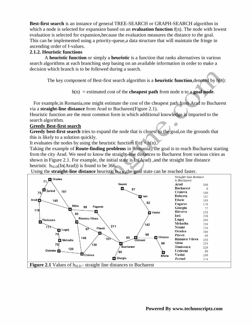
Taking the example of Route-finding problems in Romania , the goal is to reach Bucharest starting

from the city Arad. We need to know the straight-line distances to Bucharest from various cities as

shown in Figure 2.1. For example, the initial state is In(Arad) ,and the straight line distance

heuristic hSLD(In(Arad)) is found to be 366.

Using the straight-line distance heuristic hSLD ,the goal state can be reached faster.

Figure 2.1 Values of hSLD - straight line distances to Bucharest


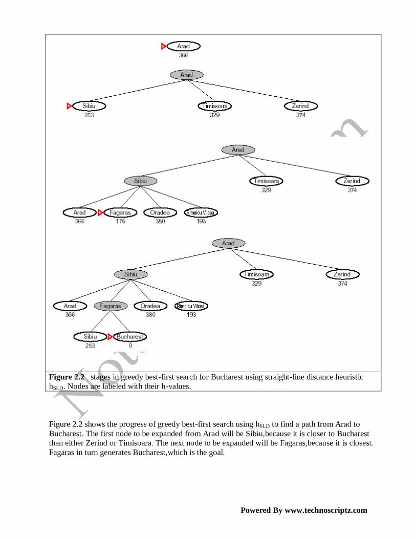
Figure 2.2 stages in greedy best-first search for Bucharest using straight-line distance heuristic

hSLD. Nodes are labeled with their h-values.

Figure 2.2 shows the progress of greedy best-first search using hSLD to find a path from Arad to

Bucharest. The first node to be expanded from Arad will be Sibiu,because it is closer to Bucharest

than either Zerind or Timisoara. The next node to be expanded will be Fagaras,because it is closest.

Fagaras in turn generates Bucharest,which is the goal.


Properties of greedy search

o Complete?? No–can get stuck in loops, e.g.,

Iasi ! Neamt ! Iasi ! Neamt !

Complete in finite space with repeated-state checking

o Time?? O(bm), but a good heuristic can give dramatic improvement

o Space?? O(bm)—keeps all nodes in memory

o Optimal?? No

Greedy best-first search is not optimal,and it is incomplete.

The worst-case time and space complexity is O(bm),where m is the maximum depth of the search

space.

A* Search

A* Search is the most widely used form of best-first search. The evaluation function f(n) is

obtained by combining

(1) g(n) = the cost to reach the node,and

(2) h(n) = the cost to get from the node to the goal :

f(n) = g(n) + h(n). A

* Search is both optimal and complete. A

* is optimal if h(n) is an admissible heuristic. The obvious

example of admissible heuristic is the straight-line distance hSLD. It cannot be an overestimate.

A* Search is optimal if h(n) is an admissible heuristic – that is,provided that h(n) never

overestimates the cost to reach the goal.

An obvious example of an admissible heuristic is the straight-line distance hSLD that we used in

getting to Bucharest. The progress of an A* tree search for Bucharest is shown in Figure 2.2.

The values of ‗g ‗ are computed from the step costs shown in the Romania map( figure 2.1). Also

the values of hSLD are given in Figure 2.1.

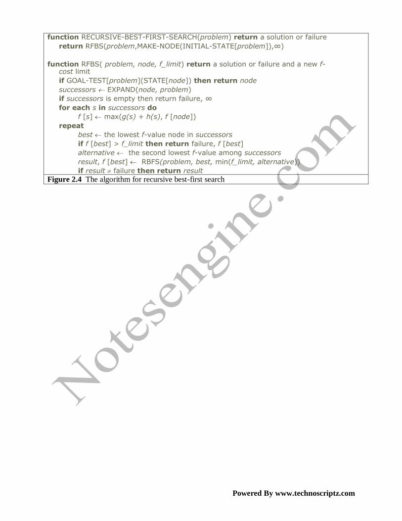
Recursive Best-first Search(RBFS) Recursive best-first search is a simple recursive algorithm that attempts to mimic the operation of

standard best-first search,but using only linear space. The algorithm is shown in figure 2.4.

Its structure is similar to that of recursive depth-first search,but rather than continuing indefinitely

down the current path,it keeps track of the f-value of the best alternative path available from any

ancestor of the current node. If the current node exceeds this limit,the recursion unwinds back to the

alternative path. As the recursion unwinds,RBFS replaces the f-value of each node along the path

with the best f-value of its children.

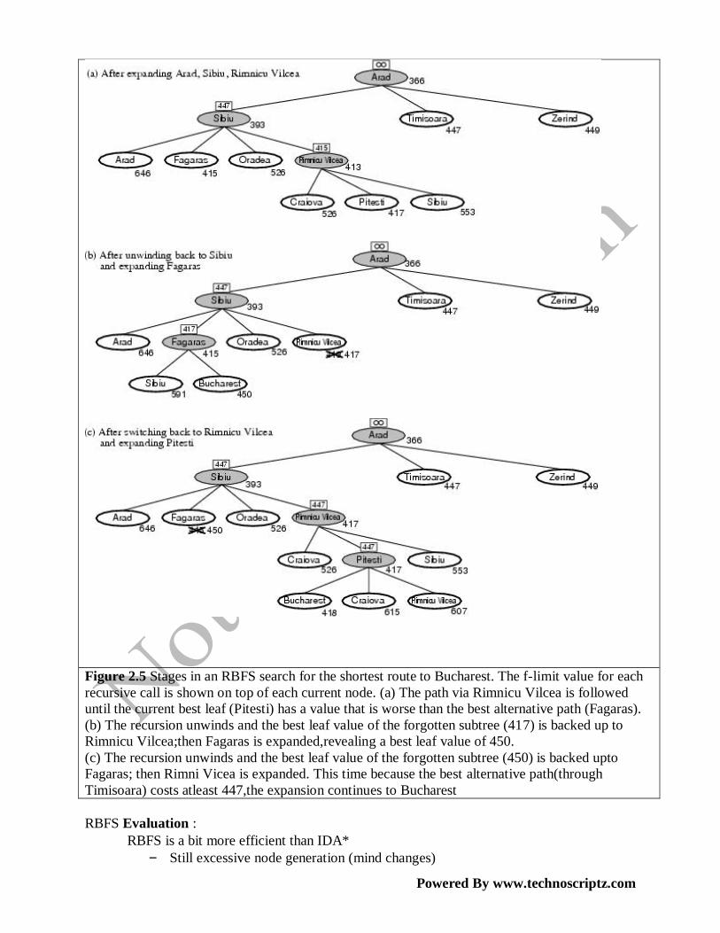
Figure 2.5 shows how RBFS reaches Bucharest.


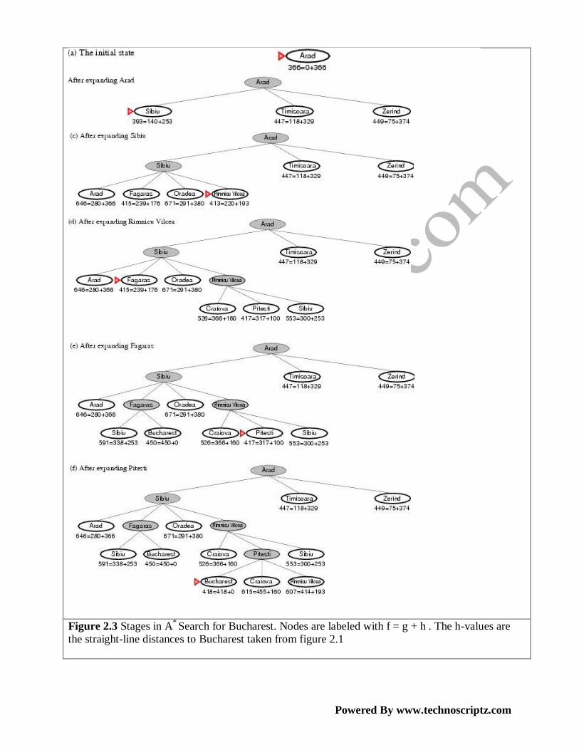
Figure 2.3 Stages in A* Search for Bucharest. Nodes are labeled with f = g + h . The h-values are

the straight-line distances to Bucharest taken from figure 2.1


function RECURSIVE-BEST-FIRST-SEARCH(problem) return a solution or failure

return RFBS(problem,MAKE-NODE(INITIAL-STATE[problem]),∞)

function RFBS( problem, node, f_limit) return a solution or failure and a new f-cost limit

if GOAL-TEST[problem](STATE[node]) then return node

successors EXPAND(node, problem)

if successors is empty then return failure, ∞

for each s in successors do

f [s] max(g(s) + h(s), f [node])

repeat

best the lowest f-value node in successors

if f [best] > f_limit then return failure, f [best]

alternative the second lowest f-value among successors

result, f [best] RBFS(problem, best, min(f_limit, alternative))

if result failure then return result Figure 2.4 The algorithm for recursive best-first search


Figure 2.5 Stages in an RBFS search for the shortest route to Bucharest. The f-limit value for each

recursive call is shown on top of each current node. (a) The path via Rimnicu Vilcea is followed

until the current best leaf (Pitesti) has a value that is worse than the best alternative path (Fagaras).

(b) The recursion unwinds and the best leaf value of the forgotten subtree (417) is backed up to

Rimnicu Vilcea;then Fagaras is expanded,revealing a best leaf value of 450.

(c) The recursion unwinds and the best leaf value of the forgotten subtree (450) is backed upto

Fagaras; then Rimni Vicea is expanded. This time because the best alternative path(through

Timisoara) costs atleast 447,the expansion continues to Bucharest

RBFS Evaluation :

RBFS is a bit more efficient than IDA*

– Still excessive node generation (mind changes)


Like A*, optimal if h(n) is admissible

Space complexity is O(bd).

– IDA* retains only one single number (the current f-cost limit)

Time complexity difficult to characterize

– Depends on accuracy if h(n) and how often best path changes.

IDA* en RBFS suffer from too little memory.

2.1.2 Heuristic Functions A heuristic function or simply a heuristic is a function that ranks alternatives in various search

algorithms at each branching step basing on an available information in order to make a decision

which branch is to be followed during a search

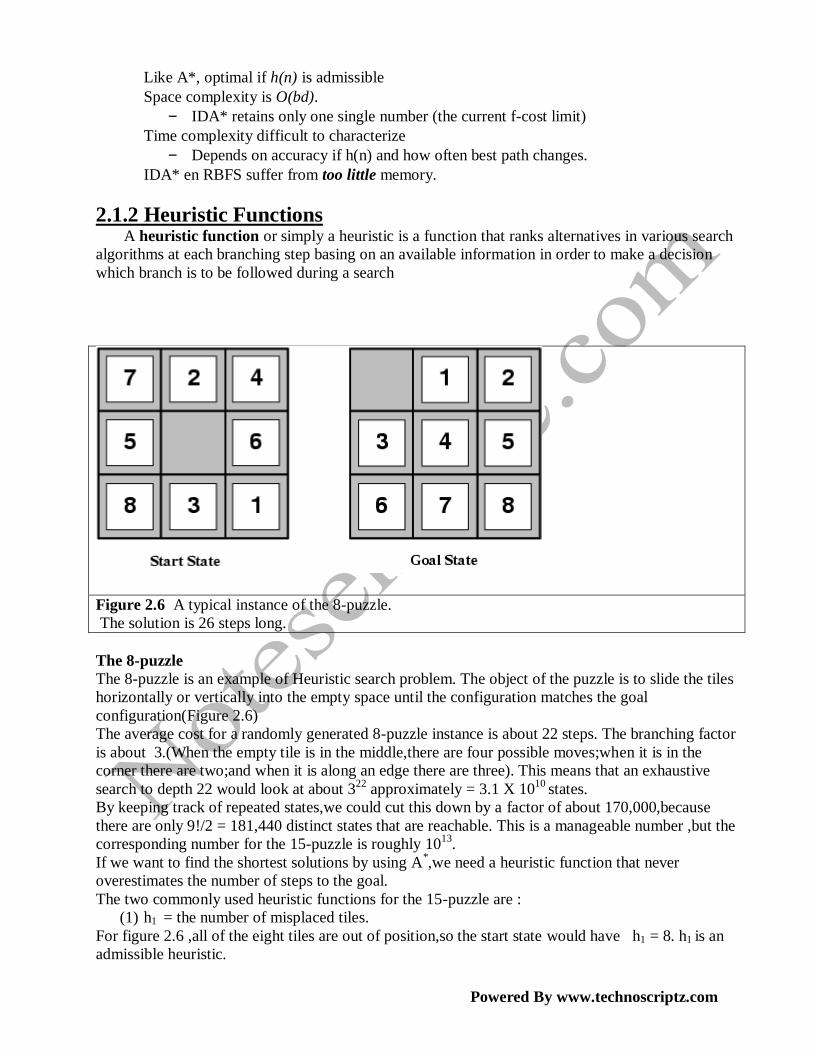
Figure 2.6 A typical instance of the 8-puzzle.

The solution is 26 steps long.

The 8-puzzle

The 8-puzzle is an example of Heuristic search problem. The object of the puzzle is to slide the tiles

horizontally or vertically into the empty space until the configuration matches the goal

configuration(Figure 2.6)

The average cost for a randomly generated 8-puzzle instance is about 22 steps. The branching factor

is about 3.(When the empty tile is in the middle,there are four possible moves;when it is in the

corner there are two;and when it is along an edge there are three). This means that an exhaustive

search to depth 22 would look at about 322

approximately = 3.1 X 1010

states.

By keeping track of repeated states,we could cut this down by a factor of about 170,000,because

there are only 9!/2 = 181,440 distinct states that are reachable. This is a manageable number ,but the

corresponding number for the 15-puzzle is roughly 1013

.

If we want to find the shortest solutions by using A*,we need a heuristic function that never

overestimates the number of steps to the goal.

The two commonly used heuristic functions for the 15-puzzle are :

(1) h1 = the number of misplaced tiles.

For figure 2.6 ,all of the eight tiles are out of position,so the start state would have h1 = 8. h1 is an

admissible heuristic.


(2) h2 = the sum of the distances of the tiles from their goal positions. This is called the city

block distance or Manhattan distance.

h2 is admissible ,because all any move can do is move one tile one step closer to the goal.

Tiles 1 to 8 in start state give a Manhattan distance of

h2 = 3 + 1 + 2 + 2 + 2 + 3 + 3 + 2 = 18.

Neither of these overestimates the true solution cost ,which is 26.

The Effective Branching factor

One way to characterize the quality of a heuristic is the effective branching factor b*. If the total

number of nodes generated by A* for a particular problem is N,and the solution depth is d,then b*

is the branching factor that a uniform tree of depth d would have to have in order to contain N+1

nodes. Thus,

N + 1 = 1 + b* + (b

*)

2+…+(b

*)

d

For example,if A* finds a solution at depth 5 using 52 nodes,then effective branching factor is 1.92.

A well designed heuristic would have a value of b* close to 1,allowing failru large problems to be

solved.

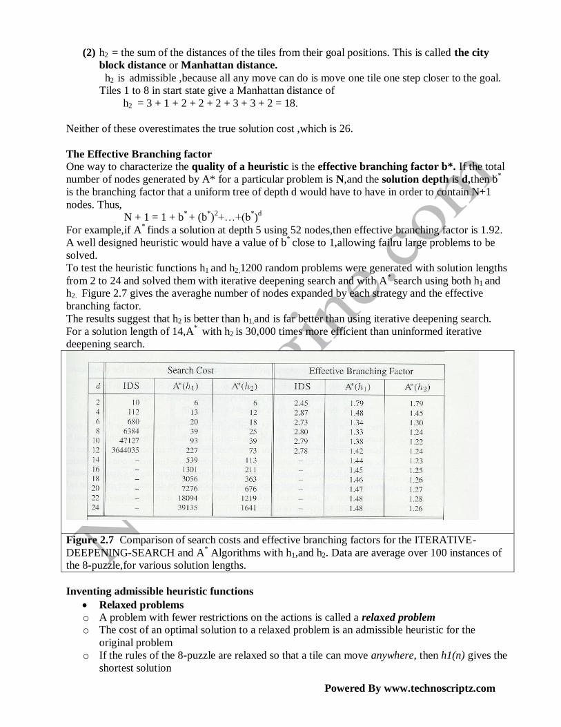
To test the heuristic functions h1 and h2,1200 random problems were generated with solution lengths

from 2 to 24 and solved them with iterative deepening search and with A* search using both h1 and

h2. Figure 2.7 gives the averaghe number of nodes expanded by each strategy and the effective

branching factor.

The results suggest that h2 is better than h1,and is far better than using iterative deepening search.

For a solution length of 14,A* with h2 is 30,000 times more efficient than uninformed iterative

deepening search.

Figure 2.7 Comparison of search costs and effective branching factors for the ITERATIVE-

DEEPENING-SEARCH and A* Algorithms with h1,and h2. Data are average over 100 instances of

the 8-puzzle,for various solution lengths.

Inventing admissible heuristic functions

Relaxed problems

o A problem with fewer restrictions on the actions is called a relaxed problem

o The cost of an optimal solution to a relaxed problem is an admissible heuristic for the

original problem

o If the rules of the 8-puzzle are relaxed so that a tile can move anywhere, then h1(n) gives the

shortest solution


o If the rules are relaxed so that a tile can move to any adjacent square, then h2(n) gives the

shortest solution

2.1.3 LOCAL SEARCH ALGORITHMS AND OPTIMIZATION

PROBLEMS o In many optimization problems, the path to the goal is irrelevant; the goal state itself is the

solution

o For example,in the 8-queens problem,what matters is the final configuration of queens,not

the order in which they are added.

o In such cases, we can use local search algorithms. They operate using a single current

state(rather than multiple paths) and generally move only to neighbors of that state.

o The important applications of these class of problems are (a) integrated-circuit

design,(b)Factory-floor layout,(c) job-shop scheduling,(d)automatic

programming,(e)telecommunications network optimization,(f)Vehicle routing,and (g)

portfolio management.

Key advantages of Local Search Algorithms

(1) They use very little memory – usually a constant amount; and

(2) they can often find reasonable solutions in large or infinite(continuous) state spaces for which

systematic algorithms are unsuitable.

OPTIMIZATION PROBLEMS

Inaddition to finding goals,local search algorithms are useful for solving pure optimization

problems,in which the aim is to find the best state according to an objective function.

State Space Landscape

To understand local search,it is better explained using state space landscape as shown in figure

2.8.

A landscape has both ―location‖ (defined by the state) and ―elevation‖(defined by the value of the

heuristic cost function or objective function).

If elevation corresponds to cost,then the aim is to find the lowest valley – a global minimum; if

elevation corresponds to an objective function,then the aim is to find the highest peak – a global

maximum.

Local search algorithms explore this landscape. A complete local search algorithm always finds a

goal if one exists; an optimal algorithm always finds a global minimum/maximum.


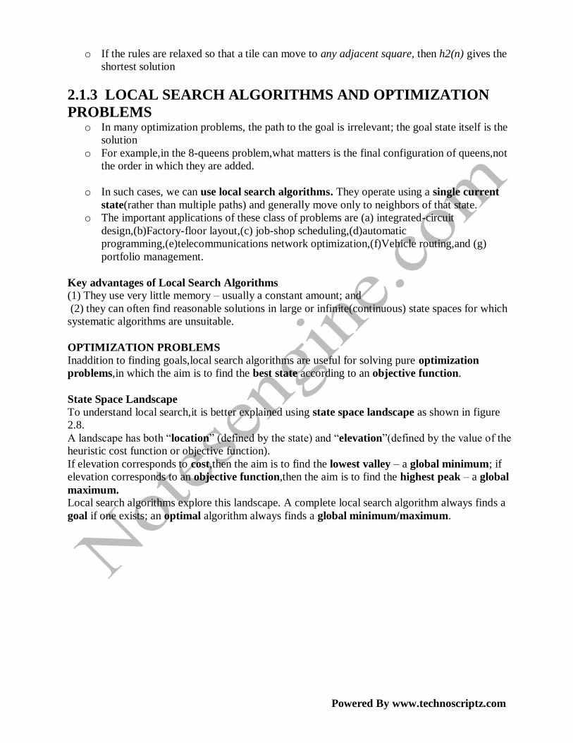
Figure 2.8 A one dimensional state space landscape in which elevation corresponds to the

objective function. The aim is to find the global maximum. Hill climbing search modifies the

current state to try to improve it ,as shown by the arrow. The various topographic features are

defined in the text

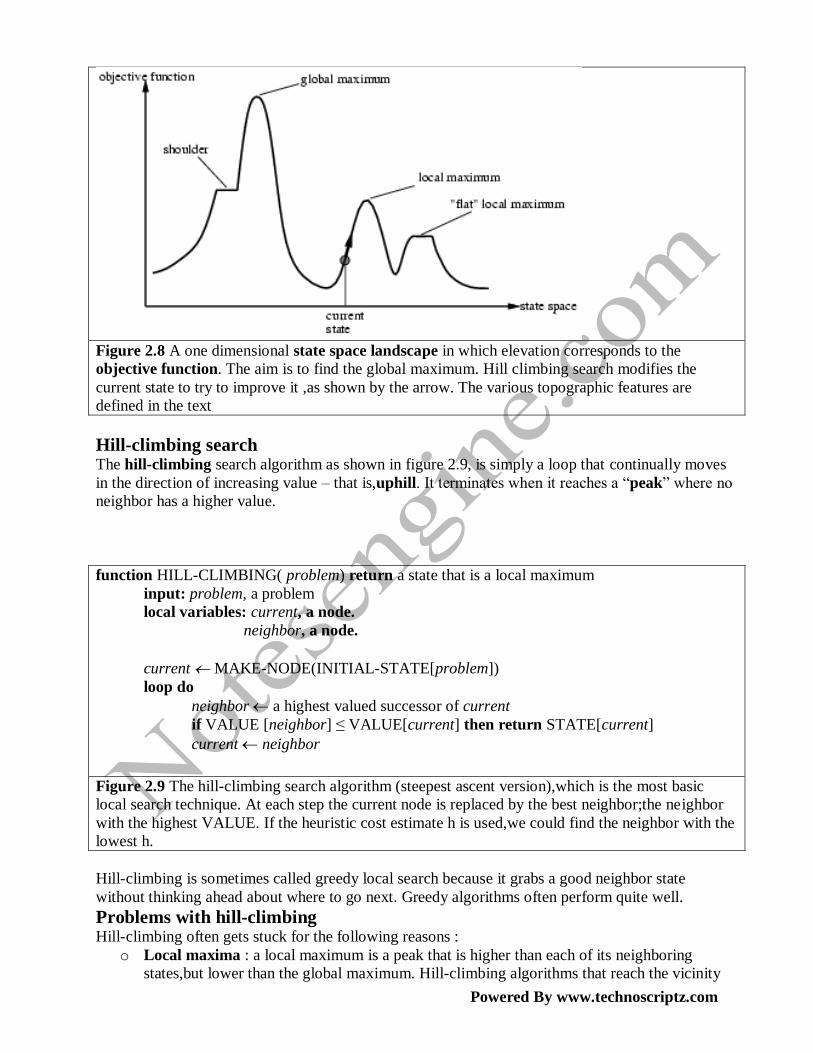
Hill-climbing search The hill-climbing search algorithm as shown in figure 2.9, is simply a loop that continually moves

in the direction of increasing value – that is,uphill. It terminates when it reaches a ―peak‖ where no

neighbor has a higher value.

function HILL-CLIMBING( problem) return a state that is a local maximum

input: problem, a problem

local variables: current, a node.

neighbor, a node.

current MAKE-NODE(INITIAL-STATE[problem])

loop do

neighbor a highest valued successor of current

if VALUE [neighbor] ≤ VALUE[current] then return STATE[current]

current neighbor

Figure 2.9 The hill-climbing search algorithm (steepest ascent version),which is the most basic

local search technique. At each step the current node is replaced by the best neighbor;the neighbor

with the highest VALUE. If the heuristic cost estimate h is used,we could find the neighbor with the

lowest h.

Hill-climbing is sometimes called greedy local search because it grabs a good neighbor state

without thinking ahead about where to go next. Greedy algorithms often perform quite well.

Problems with hill-climbing Hill-climbing often gets stuck for the following reasons :

o Local maxima : a local maximum is a peak that is higher than each of its neighboring

states,but lower than the global maximum. Hill-climbing algorithms that reach the vicinity


of a local maximum will be drawn upwards towards the peak,but will then be stuck with

nowhere else to go

o Ridges : A ridge is shown in Figure 2.10. Ridges results in a sequence of local maxima that

is very difficult for greedy algorithms to navigate.

o Plateaux : A plateau is an area of the state space landscape where the evaluation function is

flat. It can be a flat local maximum,from which no uphill exit exists,or a shoulder,from

which it is possible to make progress.

Figure 2.10 Illustration of why ridges cause difficulties for hill-climbing. The grid of states(dark

circles) is superimposed on a ridge rising from left to right,creating a sequence of local maxima that

are not directly connected to each other. From each local maximum,all th available options point

downhill.

Hill-climbing variations Stochastic hill-climbing

o Random selection among the uphill moves.

o The selection probability can vary with the steepness of the uphill move.

First-choice hill-climbing

o cfr. stochastic hill climbing by generating successors randomly until a better one is

found.

Random-restart hill-climbing

o Tries to avoid getting stuck in local maxima.

Simulated annealing search A hill-climbing algorithm that never makes ―downhill‖ moves towards states with lower value(or

higher cost) is guaranteed to be incomplete,because it can stuck on a local maximum.In contrast,a

purely random walk –that is,moving to a successor choosen uniformly at random from the set of

successors – is complete,but extremely inefficient.

Simulated annealing is an algorithm that combines hill-climbing with a random walk in someway

that yields both efficiency and completeness.

Figure 2.11 shows simulated annealing algorithm. It is quite similar to hill climbing. Instead of

picking the best move,however,it picks the random move. If the move improves the situation,it is

always accepted. Otherwise,the algorithm accepts the move with some probability less than 1. The

probability decreases exponentially with the ―badness‖ of the move – the amount E by which the

evaluation is worsened.


Simulated annealing was first used extensively to solve VLSI layout problems in the early 1980s. It

has been applied widely to factory scheduling and other large-scale optimization tasks.

Figure 2.11 The simulated annealing search algorithm,a version of stochastic hill climbing where

some downhill moves are allowed.

Genetic algorithms A Genetic algorithm(or GA) is a variant of stochastic beam search in which successor states are

generated by combining two parent states,rather than by modifying a single state.

Like beam search,Gas begin with a set of k randomly generated states,called the population. Each

state,or individual,is represented as a string over a finite alphabet – most commonly,a string of 0s

and 1s. For example,an 8 8-quuens state must specify the positions of 8 queens,each in acolumn of

8 squares,and so requires 8 x log2 8 = 24 bits.

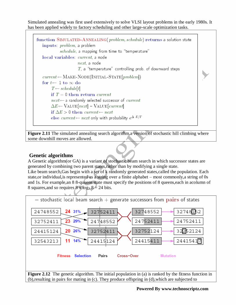
Figure 2.12 The genetic algorithm. The initial population in (a) is ranked by the fitness function in

(b),resulting in pairs for mating in (c). They produce offspring in (d),which are subjected to


mutation in (e).

Figure 2.12 shows a population of four 8-digit strings representing 8-queen states. The production

of the next generation of states is shown in Figure 2.12(b) to (e).

In (b) each state is rated by the evaluation function or the fitness function.

In (c),a random choice of two pairs is selected for reproduction,in accordance with the probabilities

in (b).

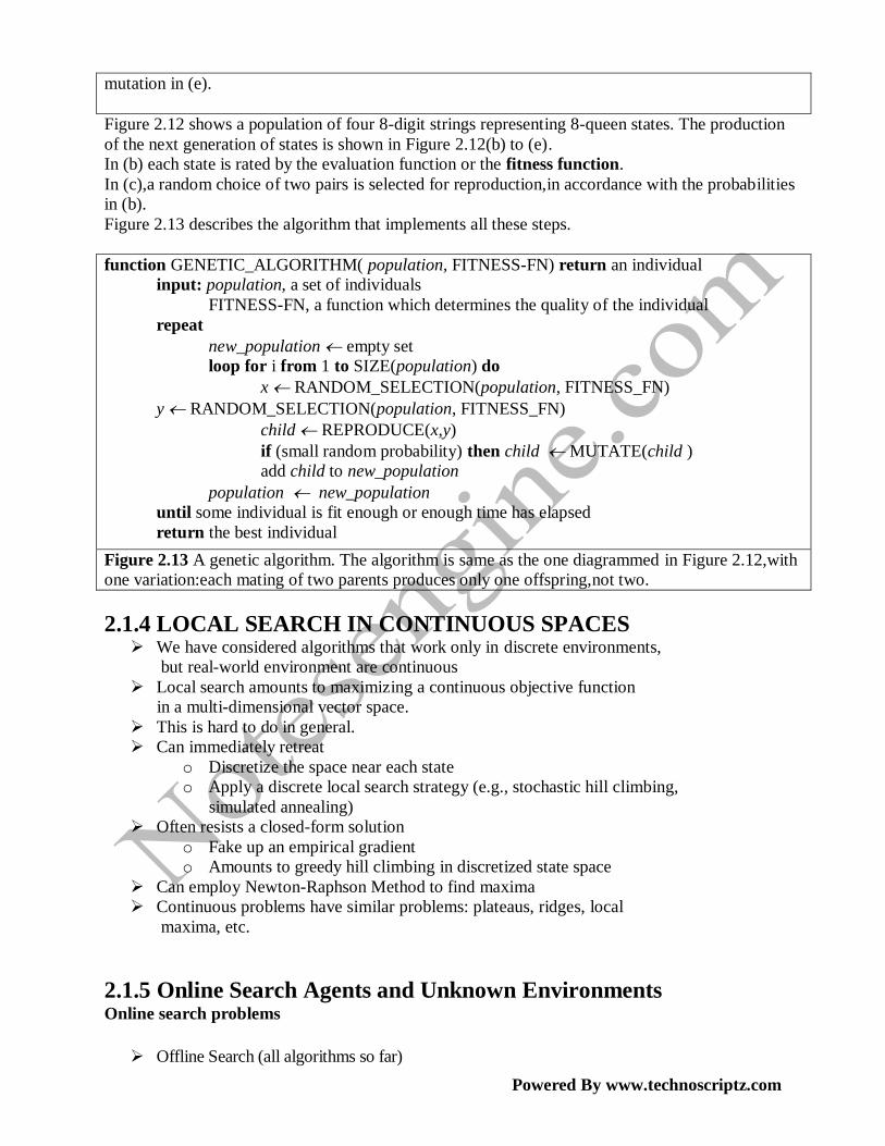
Figure 2.13 describes the algorithm that implements all these steps.

function GENETIC_ALGORITHM( population, FITNESS-FN) return an individual

input: population, a set of individuals

FITNESS-FN, a function which determines the quality of the individual

repeat

new_population empty set

loop for i from 1 to SIZE(population) do

x RANDOM_SELECTION(population, FITNESS_FN)

y RANDOM_SELECTION(population, FITNESS_FN)

child REPRODUCE(x,y)

if (small random probability) then child MUTATE(child )

add child to new_population

population new_population

until some individual is fit enough or enough time has elapsed

return the best individual

Figure 2.13 A genetic algorithm. The algorithm is same as the one diagrammed in Figure 2.12,with

one variation:each mating of two parents produces only one offspring,not two.

2.1.4 LOCAL SEARCH IN CONTINUOUS SPACES We have considered algorithms that work only in discrete environments,

but real-world environment are continuous

Local search amounts to maximizing a continuous objective function

in a multi-dimensional vector space.

This is hard to do in general.

Can immediately retreat

o Discretize the space near each state

o Apply a discrete local search strategy (e.g., stochastic hill climbing,

simulated annealing)

Often resists a closed-form solution

o Fake up an empirical gradient

o Amounts to greedy hill climbing in discretized state space

Can employ Newton-Raphson Method to find maxima

Continuous problems have similar problems: plateaus, ridges, local

maxima, etc.

2.1.5 Online Search Agents and Unknown Environments Online search problems

Offline Search (all algorithms so far)


Compute complete solution, ignoring environment Carry out action sequence

Online Search

Interleave computation and action Compute—Act—Observe—Compute—·

Online search good

For dynamic, semi-dynamic, stochastic domains Whenever offline search would yield exponentially many contingencies

Online search necessary for exploration problem

States and actions unknown to agent Agent uses actions as experiments to determine what to do

Examples Robot exploring unknown building

Classical hero escaping a labyrinth

Assume agent knows Actions available in state s

Step-cost function c(s,a,s′)

State s is a goal state When it has visited a state s previously Admissible heuristic function

h(s )

Note that agent doesn‘t know outcome state (s ′ ) for a given action (a) until it tries the action

(and all actions from a state s )

Competitive ratio compares actual cost with cost agent would follow if it knew the search space

No agent can avoid dead ends in all state spaces

Robotics examples: Staircase, ramp, cliff, terrain

Assume state space is safely explorable—some goal state is always reachable

Online Search Agents

Interleaving planning and acting hamstrings offline search

A* expands arbitrary nodes without waiting for outcome of action Online

algorithm can expand only the node it physically occupies Best to explore

nodes in physically local order Suggests using depth-first search Next node always a child of the current

When all actions have been tried, can‘t just drop state

Agent must physically backtrack

Online Depth-First Search

May have arbitrarily bad competitive ratio (wandering past goal) Okay for exploration; bad for minimizing path cost

Online Iterative-Deepening Search

Competitive ratio stays small for state space a uniform tree

Online Local Search

Hill Climbing Search Also has physical locality in node expansions

Is, in fact, already an online search algorithm Local maxima problematic: can‘t randomly transport agent to new state in


effort to escape local maximum

Random Walk as alternative Select action at random from current state Will eventually find a goal node in a finite space Can be very slow, esp. if ―backward‖ steps as common as ―forward‖

Hill Climbing with Memory instead of randomness Store ―current best estimate‖ of cost to goal at each visited state Starting

estimate is just h(s ) Augment estimate based on experience in the state space Tends to

―flatten out‖ local minima, allowing progress Employ optimism under uncertainty

Untried actions assumed to have least-possible cost Encourage exploration of untried paths

Learning in Online Search

o Rampant ignorance a ripe opportunity for learning Agent learns a ―map‖

of the environment

o Outcome of each action in each state

o Local search agents improve evaluation function accuracy

o Update estimate of value at each visited state

o Would like to infer higher-level domain model

o Example: ―Up‖ in maze search increases y -coordinate Requires o Formal way to represent and manipulate such general rules (so far, have hidden rules

within the successor function) o Algorithms that can construct general rules based on observations of the effect of

actions

2.2 CONSTRAINT SATISFACTION PROBLEMS(CSP)

A Constraint Satisfaction Problem(or CSP) is defined by a set of variables ,X1,X2,….Xn,and

a set of constraints C1,C2,…,Cm. Each variable Xi has a nonempty domain D,of possible values.

Each constraint Ci involves some subset of variables and specifies the allowable combinations of

values for that subset.

A State of the problem is defined by an assignment of values to some or all of the variables,{Xi =

vi,Xj = vj,…}. An assignment that does not violate any constraints is called a consistent or legal

assignment. A complete assignment is one in which every variable is mentioned,and a solution to a

CSP is a complete assignment that satisfies all the constraints.

Some CSPs also require a solution that maximizes an objective function.

Example for Constraint Satisfaction Problem :

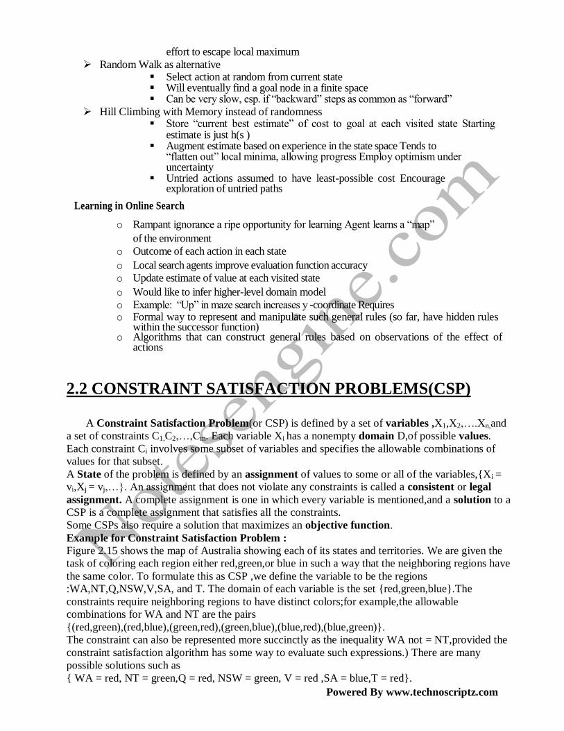
Figure 2.15 shows the map of Australia showing each of its states and territories. We are given the

task of coloring each region either red,green,or blue in such a way that the neighboring regions have

the same color. To formulate this as CSP ,we define the variable to be the regions

:WA,NT,Q,NSW,V,SA, and T. The domain of each variable is the set {red,green,blue}.The

constraints require neighboring regions to have distinct colors;for example,the allowable

combinations for WA and NT are the pairs

{(red,green),(red,blue),(green,red),(green,blue),(blue,red),(blue,green)}.

The constraint can also be represented more succinctly as the inequality WA not = NT,provided the

constraint satisfaction algorithm has some way to evaluate such expressions.) There are many

possible solutions such as

{ WA = red, NT = green,Q = red, NSW = green, V = red ,SA = blue,T = red}.


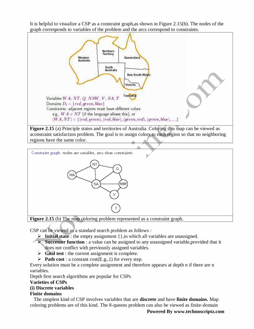
It is helpful to visualize a CSP as a constraint graph,as shown in Figure 2.15(b). The nodes of the

graph corresponds to variables of the problem and the arcs correspond to constraints.

Figure 2.15 (a) Principle states and territories of Australia. Coloring this map can be viewed as

aconstraint satisfaction problem. The goal is to assign colors to each region so that no neighboring

regions have the same color.

Figure 2.15 (b) The map coloring problem represented as a constraint graph.

CSP can be viewed as a standard search problem as follows :

Initial state : the empty assignment {},in which all variables are unassigned.

Successor function : a value can be assigned to any unassigned variable,provided that it

does not conflict with previously assigned variables.

Goal test : the current assignment is complete.

Path cost : a constant cost(E.g.,1) for every step.

Every solution must be a complete assignment and therefore appears at depth n if there are n

variables.

Depth first search algorithms are popular for CSPs

Varieties of CSPs

(i) Discrete variables

Finite domains

The simplest kind of CSP involves variables that are discrete and have finite domains. Map

coloring problems are of this kind. The 8-queens problem can also be viewed as finite-domain


CSP,where the variables Q1,Q2,…..Q8 are the positions each queen in columns 1,….8 and each

variable has the domain {1,2,3,4,5,6,7,8}. If the maximum domain size of any variable in a CSP is

d,then the number of possible complete assignments is O(dn) – that is,exponential in the number of

variables. Finite domain CSPs include Boolean CSPs,whose variables can be either true or false.

Infinite domains

Discrete variables can also have infinite domains – for example,the set of integers or the set of

strings. With infinite domains,it is no longer possible to describe constraints by enumerating all

allowed combination of values. Instead a constraint language of algebric inequalities such as

Startjob1 + 5 <= Startjob3.

(ii) CSPs with continuous domains

CSPs with continuous domains are very common in real world. For example ,in operation research

field,the scheduling of experiments on the Hubble Telescope requires very precise timing of

observations; the start and finish of each observation and maneuver are continuous-valued variables

that must obey a variety of astronomical,precedence and power constraints. The best known

category of continuous-domain CSPs is that of linear programming problems,where the

constraints must be linear inequalities forming a convex region. Linear programming problems can

be solved in time polynomial in the number of variables.

Varieties of constraints :

(i) unary constraints involve a single variable.

Example : SA # green

(ii) Binary constraints involve paris of variables.

Example : SA # WA

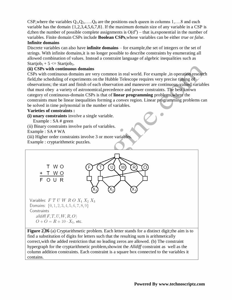
(iii) Higher order constraints involve 3 or more variables.

Example : cryptarithmetic puzzles.

Figure 2.16 (a) Cryptarithmetic problem. Each letter stands for a distinct digit;the aim is to

find a substitution of digits for letters such that the resulting sum is arithmetically

correct,with the added restriction that no leading zeros are allowed. (b) The constraint

hypergraph for the cryptarithmetic problem,showint the Alldiff constraint as well as the

column addition constraints. Each constraint is a square box connected to the variables it

contains.


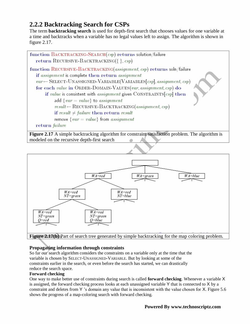
2.2.2 Backtracking Search for CSPs The term backtracking search is used for depth-first search that chooses values for one variable at

a time and backtracks when a variable has no legal values left to assign. The algorithm is shown in

figure 2.17.

Figure 2.17 A simple backtracking algorithm for constraint satisfaction problem. The algorithm is

modeled on the recursive depth-first search

Figure 2.17(b) Part of search tree generated by simple backtracking for the map coloring problem.

Propagating information through constraints So far our search algorithm considers the constraints on a variable only at the time that the

variable is chosen by SELECT-UNASSIGNED-VARIABLE. But by looking at some of the

constraints earlier in the search, or even before the search has started, we can drastically reduce the search space.

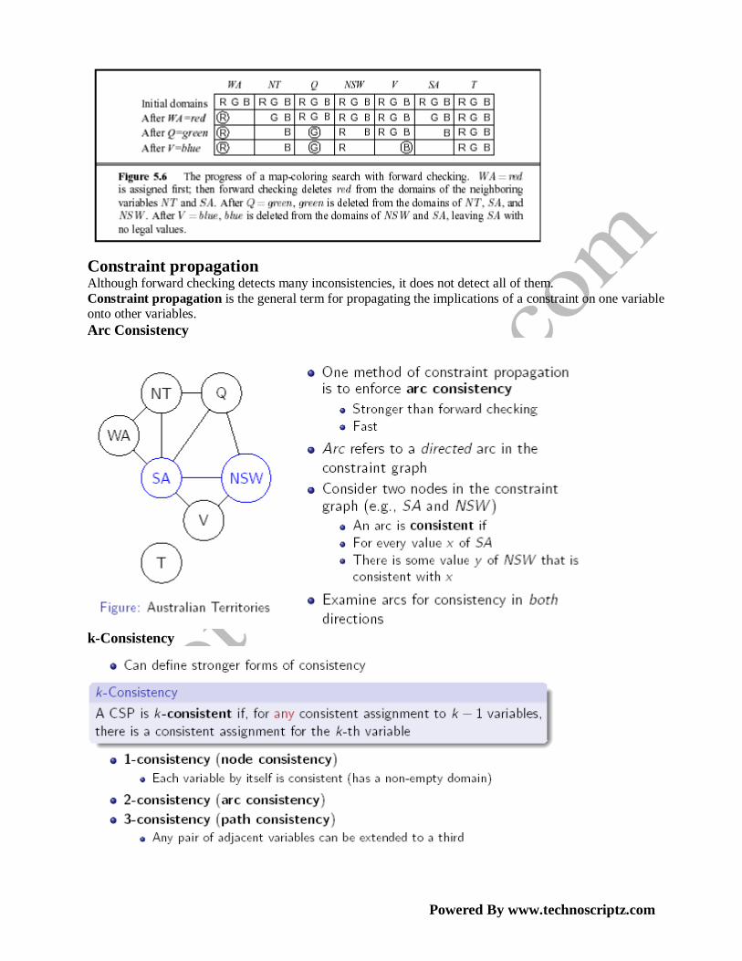
Forward checking

One way to make better use of constraints during search is called forward checking. Whenever a variable X is assigned, the forward checking process looks at each unassigned variable Y that is connected to X by a

constraint and deletes from Y ‘s domain any value that is inconsistent with the value chosen for X. Figure 5.6

shows the progress of a map-coloring search with forward checking.


Constraint propagation Although forward checking detects many inconsistencies, it does not detect all of them.

Constraint propagation is the general term for propagating the implications of a constraint on one variable onto other variables.

Arc Consistency

k-Consistency


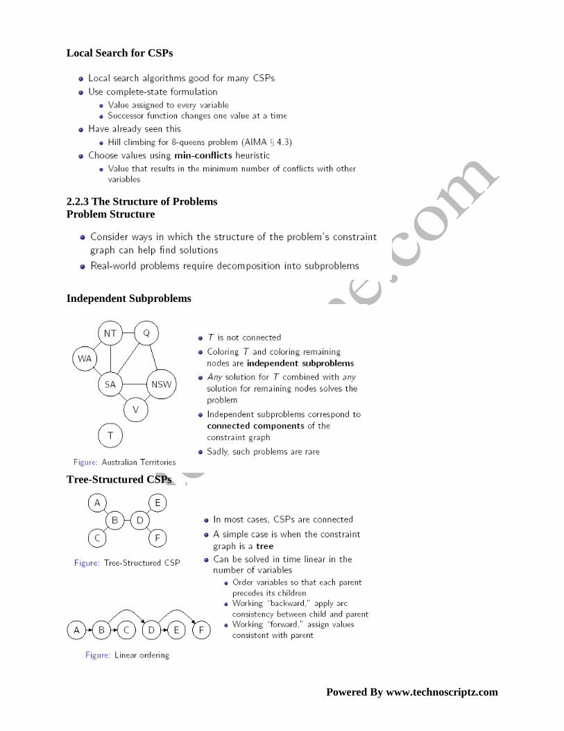
Local Search for CSPs

2.2.3 The Structure of Problems

Problem Structure

Independent Subproblems

Tree-Structured CSPs


2.4 ADVERSARIAL SEARCH Competetive environments,in which the agent‘s goals are in conflict,give rise to adversarial search

problems – often known as games.

2.4.1 Games Mathematical Game Theory,a branch of economics,views any multiagent environment as a game

provided that the impact of each agent on the other is ―significant‖,regardless of whether the agents

are cooperative or competitive. In,AI,‖games‖ are deterministic,turn-taking,two-player,zero-sum

games of perfect information. This means deterministic,fully observable environments in which

there are two agents whose actions must alternate and in which the utility values at the end of the

game are always equal and opposite. For example,if one player wins the game of chess(+1),the

other player necessarily loses(-1). It is this opposition between the agents‘ utility functions that

makes the situation adversarial.

Formal Definition of Game

We will consider games with two players,whom we will call MAX and MIN. MAX moves first,and

then they take turns moving until the game is over. At the end of the game, points are awarded to

the winning player and penalties are given to the loser. A game can be formally defined as a search

problem with the following components :

o The initial state,which includes the board position and identifies the player to move.

o A successor function,which returns a list of (move,state) pairs,each indicating a legal move

and the resulting state.

o A terminal test,which describes when the game is over. States where the game has ended

are called terminal states.

o A utility function (also called an objective function or payoff function),which give a

numeric value for the terminal states. In chess,the outcome is a win,loss,or draw,with values

+1,-1,or 0. he payoffs in backgammon range from +192 to -192.

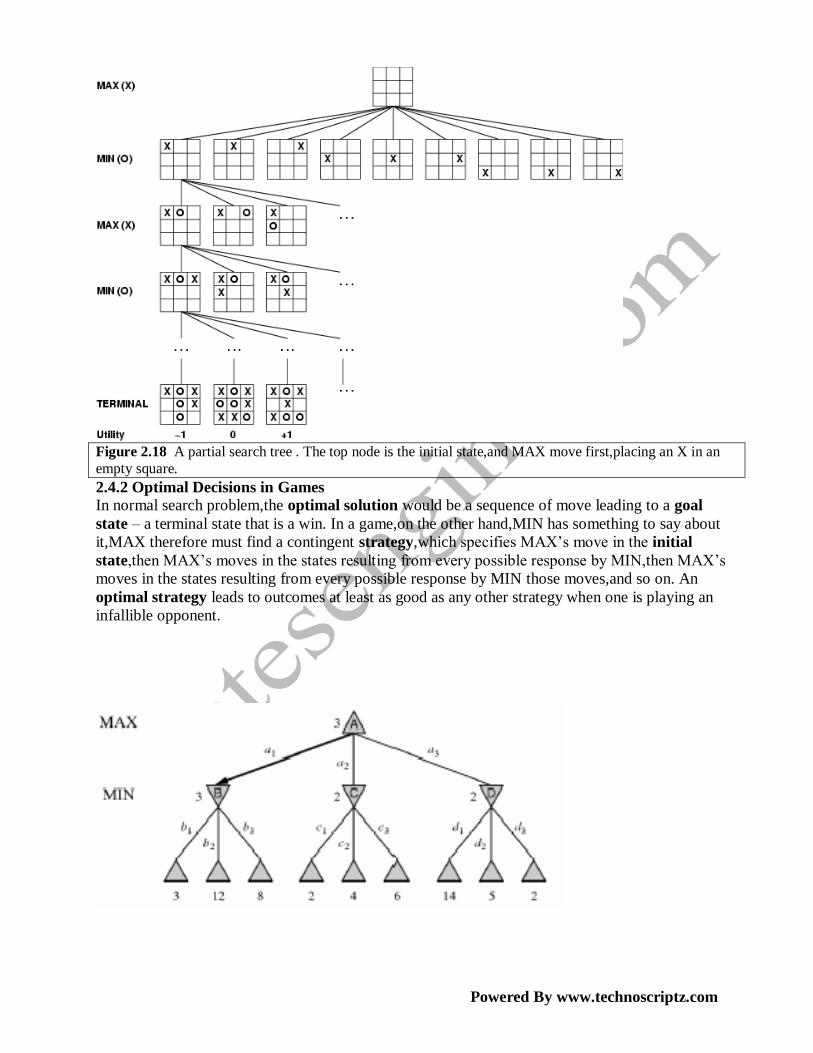
Game Tree The initial state and legal moves for each side define the game tree for the game. Figure 2.18

shows the part of the game tree for tic-tac-toe (noughts and crosses). From the initial state,MAX has

nine possible moves. Play alternates between MAX‘s placing an X and MIN‘s placing a 0 until we

reach leaf nodes corresponding to the terminal states such that one player has three in a row or all

the squares are filled. He number on each leaf node indicates the utility value of the terminal state

from the point of view of MAX;high values are assumed to be good for MAX and bad for MIN. It is

the MAX‘s job to use the search tree(particularly the utility of terminal states) to determine the best

move.


Figure 2.18 A partial search tree . The top node is the initial state,and MAX move first,placing an X in an

empty square.

2.4.2 Optimal Decisions in Games

In normal search problem,the optimal solution would be a sequence of move leading to a goal

state – a terminal state that is a win. In a game,on the other hand,MIN has something to say about

it,MAX therefore must find a contingent strategy,which specifies MAX‘s move in the initial

state,then MAX‘s moves in the states resulting from every possible response by MIN,then MAX‘s

moves in the states resulting from every possible response by MIN those moves,and so on. An

optimal strategy leads to outcomes at least as good as any other strategy when one is playing an

infallible opponent.


Figure 2.19 A two-ply game tree. The nodes are ―MAX nodes‖,in which it is AMX‘s turn to

move,and the nodes are ―MIN nodes‖. The terminal nodes show the utility values for MAX;

the other nodes are labeled with their minimax values. MAX‘s best move at the root is a1,because it

leads to the successor with the highest minimax value,and MIN‘s best reply is b1,because it leads to

the successor with the lowest minimax value.

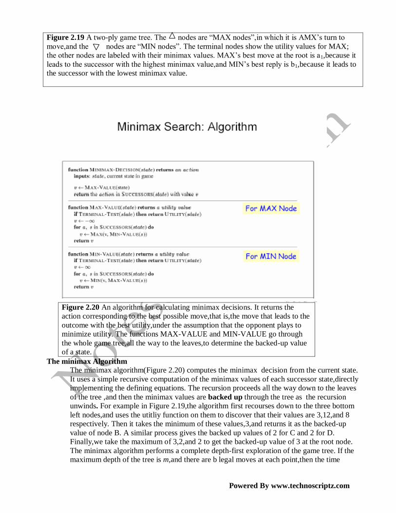
Figure 2.20 An algorithm for calculating minimax decisions. It returns the

action corresponding to the best possible move,that is,the move that leads to the

outcome with the best utility,under the assumption that the opponent plays to

minimize utility. The functions MAX-VALUE and MIN-VALUE go through

the whole game tree,all the way to the leaves,to determine the backed-up value

of a state.

The minimax Algorithm

The minimax algorithm(Figure 2.20) computes the minimax decision from the current state.

It uses a simple recursive computation of the minimax values of each successor state,directly

implementing the defining equations. The recursion proceeds all the way down to the leaves

of the tree ,and then the minimax values are backed up through the tree as the recursion

unwinds. For example in Figure 2.19,the algorithm first recourses down to the three bottom

left nodes,and uses the utitliy function on them to discover that their values are 3,12,and 8

respectively. Then it takes the minimum of these values,3,and returns it as the backed-up

value of node B. A similar process gives the backed up values of 2 for C and 2 for D.

Finally,we take the maximum of 3,2,and 2 to get the backed-up value of 3 at the root node.

The minimax algorithm performs a complete depth-first exploration of the game tree. If the

maximum depth of the tree is m,and there are b legal moves at each point,then the time


complexity of the minimax algorithm is O(bm). The space complexity is O(bm) for an

algorithm that generates successors at once.

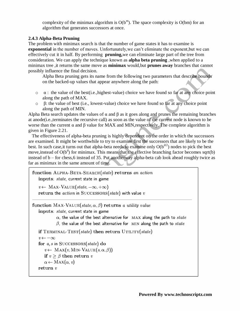
2.4.3 Alpha-Beta Pruning

The problem with minimax search is that the number of game states it has to examine is

exponential in the number of moves. Unfortunately,we can‘t eliminate the exponent,but we can

effectively cut it in half. By performing pruning,we can eliminate large part of the tree from

consideration. We can apply the technique known as alpha beta pruning ,when applied to a

minimax tree ,it returns the same move as minimax would,but prunes away branches that cannot

possibly influence the final decision.

Alpha Beta pruning gets its name from the following two parameters that describe bounds

on the backed-up values that appear anywhere along the path:

o α : the value of the best(i.e.,highest-value) choice we have found so far at any choice point

along the path of MAX.

o β: the value of best (i.e., lowest-value) choice we have found so far at any choice point

along the path of MIN.

Alpha Beta search updates the values of α and β as it goes along and prunes the remaining branches

at anode(i.e.,terminates the recursive call) as soon as the value of the current node is known to be

worse than the current α and β value for MAX and MIN,respectively. The complete algorithm is

given in Figure 2.21.

The effectiveness of alpha-beta pruning is highly dependent on the order in which the successors

are examined. It might be worthwhile to try to examine first the successors that are likely to be the

best. In such case,it turns out that alpha-beta needs to examine only O(bd/2

) nodes to pick the best

move,instead of O(bd) for minimax. This means that the effective branching factor becomes sqrt(b)

instead of b – for chess,6 instead of 35. Put anotherway alpha-beta cab look ahead roughly twice as

far as minimax in the same amount of time.


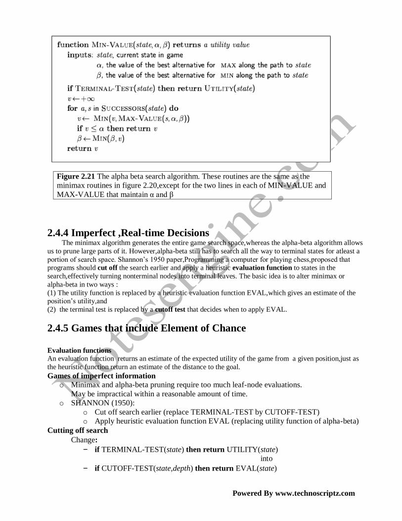
Figure 2.21 The alpha beta search algorithm. These routines are the same as the

minimax routines in figure 2.20,except for the two lines in each of MIN-VALUE and

MAX-VALUE that maintain α and β

2.4.4 Imperfect ,Real-time Decisions The minimax algorithm generates the entire game search space,whereas the alpha-beta algorithm allows

us to prune large parts of it. However,alpha-beta still has to search all the way to terminal states for atleast a

portion of search space. Shannon‘s 1950 paper,Programming a computer for playing chess,proposed that programs should cut off the search earlier and apply a heuristic evaluation function to states in the

search,effectively turning nonterminal nodes into terminal leaves. The basic idea is to alter minimax or

alpha-beta in two ways :

(1) The utility function is replaced by a heuristic evaluation function EVAL,which gives an estimate of the position‘s utility,and

(2) the terminal test is replaced by a cutoff test that decides when to apply EVAL.

2.4.5 Games that include Element of Chance

Evaluation functions An evaluation function returns an estimate of the expected utility of the game from a given position,just as

the heuristic function return an estimate of the distance to the goal.

Games of imperfect information

o Minimax and alpha-beta pruning require too much leaf-node evaluations.

May be impractical within a reasonable amount of time.

o SHANNON (1950):

o Cut off search earlier (replace TERMINAL-TEST by CUTOFF-TEST)

o Apply heuristic evaluation function EVAL (replacing utility function of alpha-beta)

Cutting off search

Change:

– if TERMINAL-TEST(state) then return UTILITY(state)

into

– if CUTOFF-TEST(state,depth) then return EVAL(state)


Introduces a fixed-depth limit depth

– Is selected so that the amount of time will not exceed what the rules of the game

allow.

When cuttoff occurs, the evaluation is performed.

Heuristic EVAL

Idea: produce an estimate of the expected utility of the game from a given position.

Performance depends on quality of EVAL.

Requirements:

– EVAL should order terminal-nodes in the same way as UTILITY.

– Computation may not take too long.

– For non-terminal states the EVAL should be strongly correlated with the actual

chance of winning.

Only useful for quiescent (no wild swings in value in near future) states

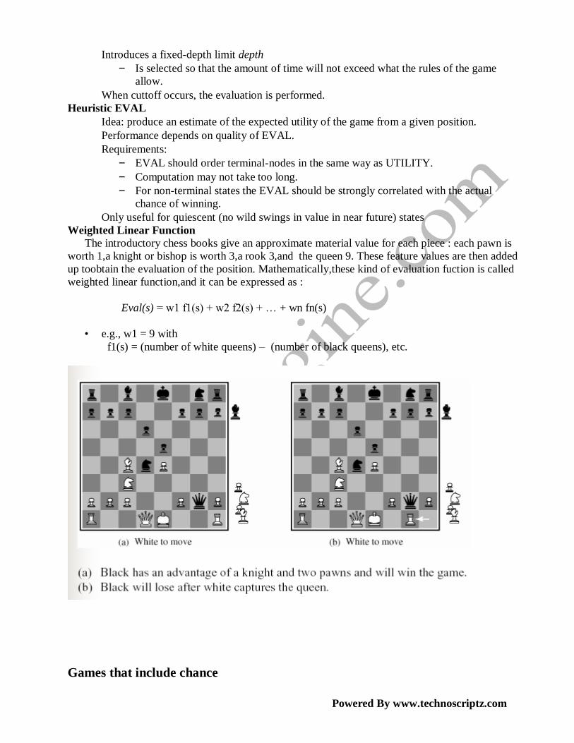
Weighted Linear Function

The introductory chess books give an approximate material value for each piece : each pawn is

worth 1,a knight or bishop is worth 3,a rook 3,and the queen 9. These feature values are then added

up toobtain the evaluation of the position. Mathematically,these kind of evaluation fuction is called

weighted linear function,and it can be expressed as :

Eval(s) = w1 f1(s) + w2 f2(s) + … + wn fn(s)

• e.g., w1 = 9 with

f1(s) = (number of white queens) – (number of black queens), etc.

Games that include chance


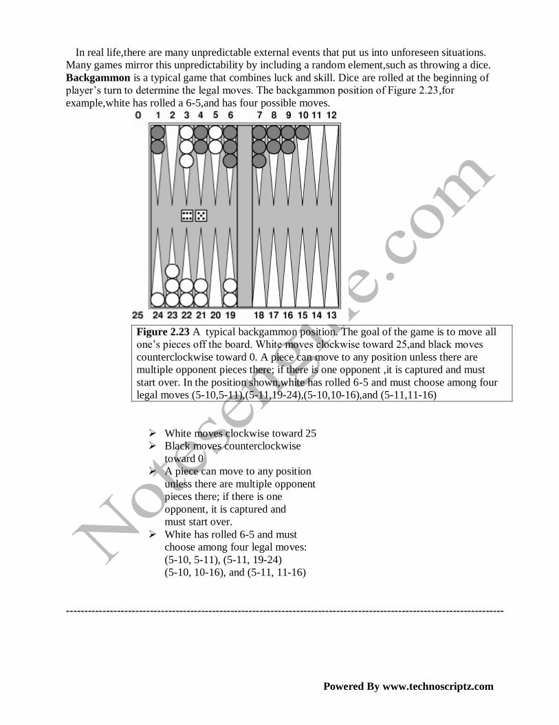
In real life,there are many unpredictable external events that put us into unforeseen situations.

Many games mirror this unpredictability by including a random element,such as throwing a dice.

Backgammon is a typical game that combines luck and skill. Dice are rolled at the beginning of

player‘s turn to determine the legal moves. The backgammon position of Figure 2.23,for

example,white has rolled a 6-5,and has four possible moves.

Figure 2.23 A typical backgammon position. The goal of the game is to move all

one‘s pieces off the board. White moves clockwise toward 25,and black moves

counterclockwise toward 0. A piece can move to any position unless there are

multiple opponent pieces there; if there is one opponent ,it is captured and must

start over. In the position shown,white has rolled 6-5 and must choose among four

legal moves (5-10,5-11),(5-11,19-24),(5-10,10-16),and (5-11,11-16)

White moves clockwise toward 25

Black moves counterclockwise

toward 0

A piece can move to any position

unless there are multiple opponent

pieces there; if there is one

opponent, it is captured and

must start over.

White has rolled 6-5 and must

choose among four legal moves:

(5-10, 5-11), (5-11, 19-24)

(5-10, 10-16), and (5-11, 11-16)

------------------------------------------------------------------------------------------------------------------------


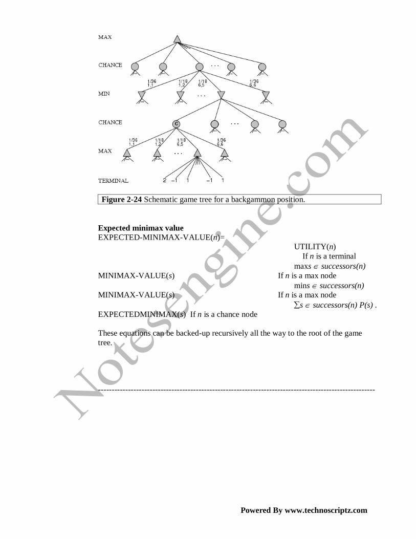
Figure 2-24 Schematic game tree for a backgammon position.

Expected minimax value

EXPECTED-MINIMAX-VALUE(n)=

UTILITY(n)

If n is a terminal

maxs successors(n)

MINIMAX-VALUE(s) If n is a max node

mins successors(n)

MINIMAX-VALUE(s) If n is a max node

s successors(n) P(s) .

EXPECTEDMINIMAX(s) If n is a chance node

These equations can be backed-up recursively all the way to the root of the game

tree.

------------------------------------------------------------------------------------------------------

(2) searching techniquescsenote.weebly.com/uploads/8/4/6/7/8467570/ai-notes-unit-ii.bak.pdf · 2.1...

Documents