2. the milky way as a galaxyrichard/astro620/schenider_mw_ch.pdf · 2. the milky way as a galaxy...
TRANSCRIPT

Peter Schneider, The Milky Way as a Galaxy.In: Peter Schneider, Extragalactic Astronomy and Cosmology. pp. 35–85 (2006)DOI: 10.1007/11614371_2 © Springer-Verlag Berlin Heidelberg 2006
35
2. The Milky Way as a GalaxyThe Earth is orbiting around the Sun, which itself isorbiting around the center of the Milky Way. Our MilkyWay, the Galaxy, is the only galaxy in which we are ableto study astrophysical processes in detail. Therefore, ourjourney through extragalactic astronomy will begin inour home Galaxy, with which we first need to becomefamiliar before we are ready to take off into the depthsof the Universe. Knowing the properties of the MilkyWay is indispensable for understanding other galaxies.
2.1 Galactic Coordinates
On a clear night, and sufficiently far away from cities,one can see the magnificent band of the Milky Wayon the sky (Fig. 2.1). This observation suggests that thedistribution of light, i.e., that of the stars in the Galaxy,is predominantly that of a thin disk. A detailed analy-sis of the geometry of the distribution of stars and gasconfirms this impression. This geometry of the Galaxysuggests the introduction of two specially adapted co-ordinate systems which are particularly convenient forquantitative descriptions.
Spherical Galactic Coordinates (�, b). We considera spherical coordinate system, with its center being“here”, at the location of the Sun (see Fig. 2.2). TheGalactic plane is the plane of the Galactic disk, i.e., itis parallel to the band of the Milky Way. The two Gal-actic coordinates � and b are angular coordinates onthe sphere. Here, b denotes the Galactic latitude, the
Fig. 2.1. An unusual op-tical image of the MilkyWay. This total view ofthe Galaxy is composedof a large number ofindividual images
angular distance of a source from the Galactic plane,with b ∈ [−90◦,+90◦]. The great circle b = 0◦ is thenlocated in the plane of the Galactic disk. The direc-tion b = 90◦ is perpendicular to the disk and denotesthe North Galactic Pole (NGP), while b = −90◦ marksthe direction to the South Galactic Pole (SGP). Thesecond angular coordinate is the Galactic longitude �,with � ∈ [0◦, 360◦]. It measures the angular separationbetween the position of a source, projected perpendic-ularly onto the Galactic disk (see Fig. 2.2), and theGalactic center, which itself has angular coordinatesb = 0◦ and � = 0◦. Given � and b for a source, its loca-tion on the sky is fully specified. In order to specify itsthree-dimensional location, the distance of that sourcefrom us is also needed.
The conversion of the positions of sources given inGalactic coordinates (b, �) to that in equatorial coordi-nates (α, δ) and vice versa is obtained from the rotationbetween these two coordinate systems, and is describedby spherical trigonometry.1 The necessary formulae canbe found in numerous standard texts. We will not re-produce them here, since nowadays this transformationis done nearly exclusively using computer programs.Instead, we will give some examples. The followingfigures refer to the Epoch 2000: due to the precession
1The equatorial coordinates are defined by the direction of the Earth’srotation axis and by the rotation of the Earth. The intersections of theEarth’s axis and the sphere define the northern and southern poles. Thegreat circles on the sphere through these two poles, the meridians, arecurves of constant right ascension α. Curves perpendicular to themand parallel to the projection of the Earth’s equator onto the sky arecurves of constant declination δ, with the poles located at δ = ±90◦.

36
2. The Milky Way as a Galaxy
Fig. 2.2. The Sun is at the origin of the Galactic coordinatesystem. The directions to the Galactic center and to the NorthGalactic Pole (NGP) are indicated and are located at � = 0◦and b = 0◦, and at b = 90◦, respectively
of the rotation axis of the Earth, the equatorial coor-dinate system changes with time, and is updated fromtime to time. The position of the Galactic center (at� = 0◦ = b) is α = 17h45.6m, δ = −28◦56.′2 in equato-rial coordinates. This immediately implies that at the LaSilla Observatory, located at geographic latitude −29◦,the Galactic center is found near the zenith at localmidnight in May/June. Because of the high stellar den-sity in the Galactic disk and the large extinction dueto dust this is therefore not a good season for extra-galactic observations from La Silla. The North GalacticPole has coordinates αNGP = 192.859 48◦ ≈ 12h51m,δNGP = 27.128 25◦ ≈ 27◦7.′7.
Zone of Avoidance. As already mentioned, the absorp-tion by dust and the presence of numerous bright starsrender optical observations of extragalactic sources inthe direction of the disk difficult. The best observingconditions are found at large |b|, while it is very hardto do extragalactic astronomy in the optical regime at|b|� 10◦; this region is therefore often called the “Zoneof Avoidance”. An illustrative example is the galaxyDwingeloo 1, which was already mentioned in Sect. 1.1(see Fig. 1.6). This galaxy was only discovered in the1990s despite being in our immediate vicinity: it islocated at low |b|, right in the Zone of Avoidance.
Cylindrical Galactic Coordinates (R,θ, z). The an-gular coordinates introduced above are well suited todescribing the angular position of a source relative to the
Galactic disk. However, we will now introduce anotherthree-dimensional coordinate system for the descrip-tion of the Milky Way geometry that will prove veryconvenient in the study of the kinematic and dynamicproperties of the Milky Way. It is a cylindrical coor-dinate system, with the Galactic center at the origin(see also Fig. 2.13). The radial coordinate R measuresthe distance of an object from the Galactic center inthe disk, and z specifies the height above the disk (ob-jects with negative z are thus located below the Galacticdisk, i.e., south of it). For instance, the Sun has a dis-tance from the Galactic center of R ≈ 8 kpc. The angleθ specifies the angular separation of an object in the diskrelative to the position of the Sun, seen from the Gal-actic center. The distance of an object with coordinatesR, θ, z from the Galactic center is then
√R2 + z2, inde-
pendent of θ. If the matter distribution in the Milky Waywere axially symmetric, the density would then dependonly on R and z, but not on θ. Since this assumptionis a good approximation, this coordinate system is verywell suited for the physical description of the Galaxy.
2.2 Determination of DistancesWithin Our Galaxy
A central problem in astronomy is the estimation of dis-tances. The position of sources on the sphere gives usa two-dimensional picture. To obtain three-dimensionalinformation, measurements of distances are required.Furthermore, we need to know the distance to a sourceif we want to draw conclusions about its physical param-eters. For example, we can directly observe the angulardiameter of an object, but to derive the physical size weneed to know its distance. Another example is the de-termination of the luminosity L of a source, which canbe derived from the observed flux S only by means ofits distance D, using
L = 4πS D2 . (2.1)
It is useful to consider the dimensions of the physicalparameters in this equation. The unit of the luminosityis [L] = erg s−1, and that of the flux [S] = erg s−1 cm−2.The flux is the energy passing through a unit area perunit time (see Appendix A). Of course, the physicalproperties of a source are characterized by the lumi-
2.2 Determination of Distances Within Our Galaxy
37
nosity L and not by the flux S, which depends on itsdistance from the Sun.
In the following section we will review various meth-ods for the estimation of distances in our Milky Way,postponing the discussion of methods for estimatingextragalactic distances to Sect. 3.6.
2.2.1 Trigonometric Parallax
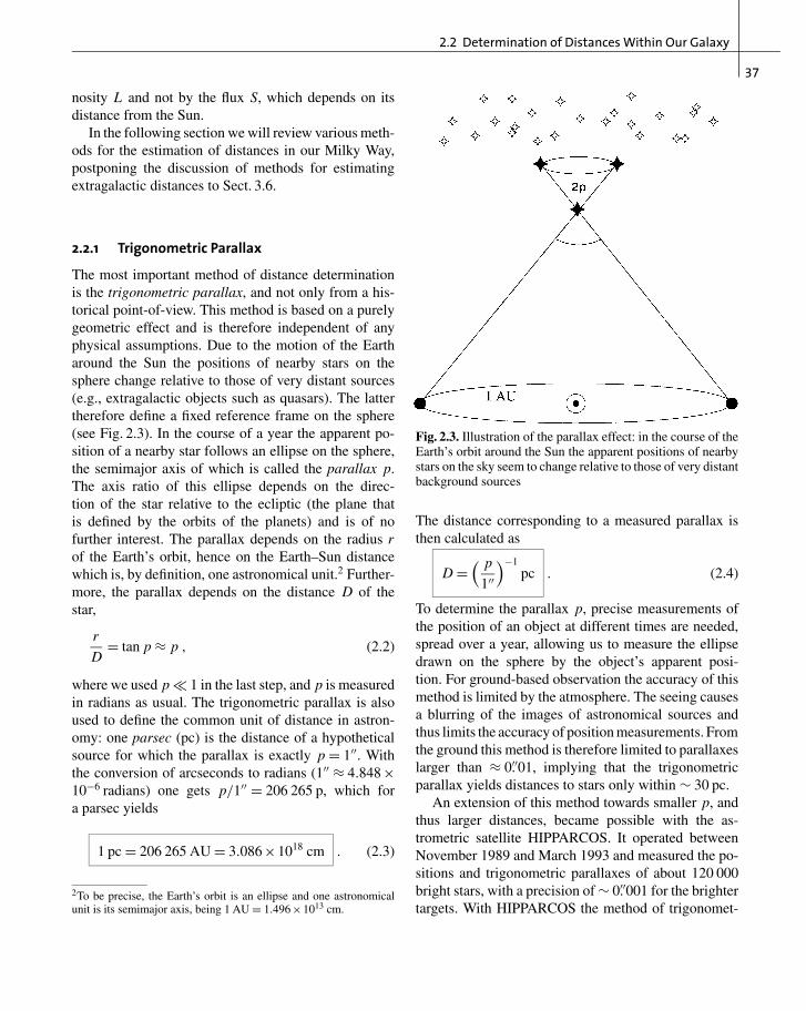
The most important method of distance determinationis the trigonometric parallax, and not only from a his-torical point-of-view. This method is based on a purelygeometric effect and is therefore independent of anyphysical assumptions. Due to the motion of the Eartharound the Sun the positions of nearby stars on thesphere change relative to those of very distant sources(e.g., extragalactic objects such as quasars). The lattertherefore define a fixed reference frame on the sphere(see Fig. 2.3). In the course of a year the apparent po-sition of a nearby star follows an ellipse on the sphere,the semimajor axis of which is called the parallax p.The axis ratio of this ellipse depends on the direc-tion of the star relative to the ecliptic (the plane thatis defined by the orbits of the planets) and is of nofurther interest. The parallax depends on the radius rof the Earth’s orbit, hence on the Earth–Sun distancewhich is, by definition, one astronomical unit.2 Further-more, the parallax depends on the distance D of thestar,
r
D= tan p ≈ p , (2.2)
where we used p 1 in the last step, and p is measuredin radians as usual. The trigonometric parallax is alsoused to define the common unit of distance in astron-omy: one parsec (pc) is the distance of a hypotheticalsource for which the parallax is exactly p = 1′′. Withthe conversion of arcseconds to radians (1′′ ≈ 4.848×10⁻⁶ radians) one gets p/1′′ = 206 265 p, which fora parsec yields
1 pc = 206 265 AU = 3.086×1018 cm . (2.3)
2To be precise, the Earth’s orbit is an ellipse and one astronomicalunit is its semimajor axis, being 1 AU = 1.496×1013 cm.
Fig. 2.3. Illustration of the parallax effect: in the course of theEarth’s orbit around the Sun the apparent positions of nearbystars on the sky seem to change relative to those of very distantbackground sources
The distance corresponding to a measured parallax isthen calculated as
D =( p
1′′)−1
pc . (2.4)
To determine the parallax p, precise measurements ofthe position of an object at different times are needed,spread over a year, allowing us to measure the ellipsedrawn on the sphere by the object’s apparent posi-tion. For ground-based observation the accuracy of thismethod is limited by the atmosphere. The seeing causesa blurring of the images of astronomical sources andthus limits the accuracy of position measurements. Fromthe ground this method is therefore limited to parallaxeslarger than ≈ 0′′. 01, implying that the trigonometricparallax yields distances to stars only within ∼ 30 pc.
An extension of this method towards smaller p, andthus larger distances, became possible with the as-trometric satellite HIPPARCOS. It operated betweenNovember 1989 and March 1993 and measured the po-sitions and trigonometric parallaxes of about 120 000bright stars, with a precision of ∼ 0′′. 001 for the brightertargets. With HIPPARCOS the method of trigonomet-

38
2. The Milky Way as a Galaxy
ric parallax could be extended to stars up to distancesof ∼ 300 pc. The satellite GAIA, the successor mis-sion to HIPPARCOS, is scheduled to be launched in2012. GAIA will compile a catalog of ∼ 109 stars upto V ≈ 20 in four broad-band and eleven narrow-bandfilters. It will measure parallaxes for these stars withan accuracy of ∼ 2×10⁻⁴ arcsec, with the accuracyfor brighter stars even being considerably better. GAIAwill thus determine the distances for ∼ 2×10⁸ starswith a precision of 10%, and tangential velocities (seenext section) with a precision of better than 3 km/s.
The trigonometric parallax method forms the basisof nearly all distance determinations owing to its purelygeometrical nature. For example, using this method thedistances to nearby stars have been determined, allow-ing the production of the Hertzsprung–Russell diagram(see Appendix B.2). Hence, all distance measures thatare based on the properties of stars, such as will bedescribed below, are calibrated by the trigonometricparallax.
2.2.2 Proper Motions
Stars are moving relative to us or, more precisely, rel-ative to the Sun. To study the kinematics of the MilkyWay we need to be able to measure the velocities ofstars. The radial component vr of the velocity is easilyobtained from the Doppler shift of spectral lines,
vr = Δλ
λ0c , (2.5)
where λ0 is the rest-frame wavelength of an atomictransition and Δλ = λobs −λ0 the Doppler shift of thewavelength due to the radial velocity of the source. Thesign of the radial velocity is defined such that vr > 0corresponds to a motion away from us, i.e., to a redshiftof spectral lines.
In contrast, the determination of the other two veloc-ity components is much more difficult. The tangentialcomponent, vt, of the velocity can be obtained from theproper motion of an object. In addition to the motioncaused by the parallax, stars also change their posi-tions on the sphere as a function of time because ofthe transverse component of their velocity relative tothe Sun. The proper motion μ is thus an angular veloc-ity, e.g., measured in milliarcseconds per year (mas/yr).
This angular velocity is linked to the tangential velocitycomponent via
vt = Dμ orvt
km/s= 4.74
(D
1 pc
)(μ
1′′/yr
).
(2.6)
Therefore, one can calculate the tangential velocity fromthe proper motion and the distance. If the latter is derivedfrom the trigonometric parallax, (2.6) and (2.4) can becombined to yield
vt
km/s= 4.74
(μ
1′′/yr
)( p
1′′)−1
. (2.7)
HIPPARCOS measured proper motions for ∼ 105 starswith an accuracy of up to a few mas/yr; however, theycan be translated into physical velocities only if theirdistance is known.
Of course, the proper motion has two components,corresponding to the absolute value of the angular ve-locity and its direction on the sphere. Together with vr
this determines the three-dimensional velocity vector.Correcting for the known velocity of the Earth aroundthe Sun, one can then compute the velocity vector v
of the star relative to the Sun, called the heliocentricvelocity.
2.2.3 Moving Cluster Parallax
The stars in an (open) star cluster all have a very similarspatial velocity. This implies that their proper motionvectors should be similar. To what extent the propermotions are aligned depends on the angular extent of thestar cluster on the sphere. Like two railway tracks thatrun parallel but do not appear parallel to us, the vectorsof proper motions in a star cluster also do not appearparallel. They are directed towards a convergence point,as depicted in Fig. 2.4. We shall demonstrate next howto use this effect to determine the distance to a starcluster.
We consider a star cluster and assume that all starshave the same spatial velocity v. The position of the i-thstar as a function of time is then described by
ri(t) = ri +vt , (2.8)
where ri is the current position if we identify the originof time, t = 0, with “today”. The direction of a star

2.2 Determination of Distances Within Our Galaxy
39
Fig. 2.4. The moving cluster parallax is a projection effect,similar to that known from viewing railway tracks. The di-rections of velocity vectors pointing away from us seem toconverge and intersect at the convergence point. The connect-ing line from the observer to the convergence point is parallelto the velocity vector of the star cluster
relative to us is described by the unit vector
ni(t) := ri(t)
|ri(t)| . (2.9)
From this, one infers that for large times, t → ∞, thedirection vectors are identical for all stars in the cluster,
ni(t) → v
|v| =: nconv . (2.10)
Hence for large times all stars will appear at the samepoint nconv: the convergence point. This only dependson the direction of the velocity vector of the star cluster.In other words, the direction vector of the stars is suchthat they are all moving towards the convergence point.Thus, nconv (and hence v/|v|) can be measured fromthe direction of the proper motions of the stars in thecluster, and so can v/|v|. On the other hand, one compo-nent of v can be determined from the (easily measured)radial velocity vr. With these two observables the three-dimensional velocity vector v is completely determined,as is easily demonstrated: let ψ be the angle between theline-of-sight n towards a star in the cluster and v. Theangle ψ is directly read off from the direction vector nand the convergence point, cos ψ = n ·v/|v| = nconv ·n.With v ≡ |v| one then obtains
vr = v cos ψ , vt = v sin ψ ,
and so
vt = vr tan ψ . (2.11)
This means that the tangential velocity vt can be mea-sured without determining the distance to the stars inthe cluster. On the other hand, (2.6) defines a relationbetween the proper motion, the distance, and vt. Hence,a distance determination for the star is now possible with
μ = vt
D= vr tan ψ
D→ D = vr tan ψ
μ. (2.12)
This method yields accurate distance estimates of starclusters within ∼ 200 pc. The accuracy depends on themeasurability of the proper motions. Furthermore, thecluster should cover a sufficiently large area on the skyfor the convergence point to be well defined. For thedistance estimate, one can then take the average overa large number of stars in the cluster if one assumes thatthe spatial extent of the cluster is much smaller than itsdistance to us. Targets for applying this method are theHyades, a cluster of about 200 stars at a mean distanceof D ≈ 45 pc, the Ursa-Major group of about 60 starsat D ≈ 24 pc, and the Pleiades with about 600 stars atD ≈ 130 pc.
Historically the distance determination to theHyades, using the moving cluster parallax, was ex-tremely important because it defined the scale to allother, larger distances. Its constituent stars of knowndistance are used to construct a calibrated Hertzsprung–Russell diagram which forms the basis for determiningthe distance to other star clusters, as will be discussed inSect. 2.2.4. In other words, it is the lowest rung of the so-called distance ladder that we will discuss in Sect. 3.6.With HIPPARCOS, however, the distance to the Hyadesstars could also be measured using the trigonometricparallax, yielding more accurate values. HIPPARCOSwas even able to differentiate the “near” from the “far”side of the cluster – this star cluster is too close for theassumption of an approximately equal distance of allits stars to be still valid. A recent value for the meandistance of the Hyades is
DHyades = 46.3±0.3 pc . (2.13)
2.2.4 Photometric Distance;Extinction and Reddening
Most stars in the color–magnitude diagram are locatedalong the main sequence. This enables us to com-pile a calibrated main sequence of those stars whose
40
2. The Milky Way as a Galaxy
trigonometric parallaxes are measured, thus with knowndistances. Utilizing photometric methods, it is then pos-sible to derive the distance to a star cluster, as we willdemonstrate in the following.
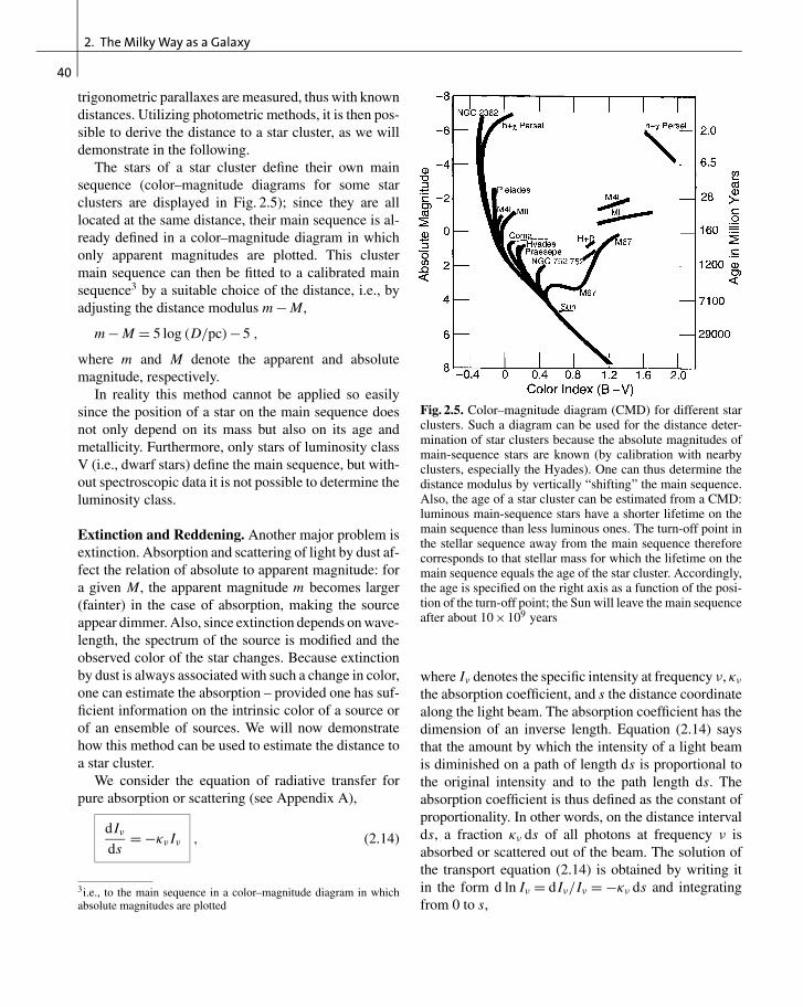
The stars of a star cluster define their own mainsequence (color–magnitude diagrams for some starclusters are displayed in Fig. 2.5); since they are alllocated at the same distance, their main sequence is al-ready defined in a color–magnitude diagram in whichonly apparent magnitudes are plotted. This clustermain sequence can then be fitted to a calibrated mainsequence3 by a suitable choice of the distance, i.e., byadjusting the distance modulus m − M,
m − M = 5 log (D/pc)−5 ,
where m and M denote the apparent and absolutemagnitude, respectively.
In reality this method cannot be applied so easilysince the position of a star on the main sequence doesnot only depend on its mass but also on its age andmetallicity. Furthermore, only stars of luminosity classV (i.e., dwarf stars) define the main sequence, but with-out spectroscopic data it is not possible to determine theluminosity class.
Extinction and Reddening. Another major problem isextinction. Absorption and scattering of light by dust af-fect the relation of absolute to apparent magnitude: fora given M, the apparent magnitude m becomes larger(fainter) in the case of absorption, making the sourceappear dimmer. Also, since extinction depends on wave-length, the spectrum of the source is modified and theobserved color of the star changes. Because extinctionby dust is always associated with such a change in color,one can estimate the absorption – provided one has suf-ficient information on the intrinsic color of a source orof an ensemble of sources. We will now demonstratehow this method can be used to estimate the distance toa star cluster.
We consider the equation of radiative transfer forpure absorption or scattering (see Appendix A),
d Iνds
= −κν Iν , (2.14)
3i.e., to the main sequence in a color–magnitude diagram in whichabsolute magnitudes are plotted
Fig. 2.5. Color–magnitude diagram (CMD) for different starclusters. Such a diagram can be used for the distance deter-mination of star clusters because the absolute magnitudes ofmain-sequence stars are known (by calibration with nearbyclusters, especially the Hyades). One can thus determine thedistance modulus by vertically “shifting” the main sequence.Also, the age of a star cluster can be estimated from a CMD:luminous main-sequence stars have a shorter lifetime on themain sequence than less luminous ones. The turn-off point inthe stellar sequence away from the main sequence thereforecorresponds to that stellar mass for which the lifetime on themain sequence equals the age of the star cluster. Accordingly,the age is specified on the right axis as a function of the posi-tion of the turn-off point; the Sun will leave the main sequenceafter about 10×109 years
where Iν denotes the specific intensity at frequency ν, κν
the absorption coefficient, and s the distance coordinatealong the light beam. The absorption coefficient has thedimension of an inverse length. Equation (2.14) saysthat the amount by which the intensity of a light beamis diminished on a path of length ds is proportional tothe original intensity and to the path length ds. Theabsorption coefficient is thus defined as the constant ofproportionality. In other words, on the distance intervalds, a fraction κν ds of all photons at frequency ν isabsorbed or scattered out of the beam. The solution ofthe transport equation (2.14) is obtained by writing itin the form d ln Iν = d Iν/Iν = −κν ds and integratingfrom 0 to s,

2.2 Determination of Distances Within Our Galaxy
41
ln Iν(s)− ln Iν(0) = −s∫
0
ds′ κν(s′) ≡ −τν(s) ,
where in the last step we defined the optical depth, τν,which depends on frequency. This yields
Iν(s) = Iν(0) e−τν(s) . (2.15)
The specific intensity is thus reduced by a factor e−τ
compared to the case of no absorption taking place.Accordingly, for the flux we obtain
Sν = Sν(0) e−τν(s) , (2.16)
where Sν is the flux measured by the observer at a dis-tance s from the source, and Sν(0) is the flux of thesource without absorption. Because of the relation be-tween flux and magnitude m = −2.5 log S + const, orS ∝ 10−0.4m , one has
Sν
Sν,0= 10−0.4(m−m0) = e−τν = 10− log(e)τν ,
or
Aν := m −m0 = −2.5 log(Sν/Sν,0)
= 2.5 log(e) τν = 1.086τν . (2.17)
Here, Aν is the extinction coefficient describing thechange of apparent magnitude m compared to that with-out absorption, m0. Since the absorption coefficient κν
depends on frequency, absorption is always linked toa change in color. This is described by the color excesswhich is defined as follows:
E(X −Y ) := AX − AY = (X − X0)− (Y −Y0)
= (X −Y )− (X −Y )0 . (2.18)
The color excess describes the change of the color index(X −Y), measured in two filters X and Y that define thecorresponding spectral windows by their transmissioncurves. The ratio AX/AY = τν(X)/τν(Y) depends only onthe optical properties of the dust or, more specifically,on the ratio of the absorption coefficients in the twofrequency bands X and Y considered here. Thus, thecolor excess is proportional to the extinction coefficient,
E(X −Y ) = AX − AY = AX
(1− AY
AX
)≡ AX R−1
X ,
(2.19)
where in the last step we introduced the factor of pro-portionality RX between the extinction coefficient andthe color excess, which depends only on the propertiesof the dust and the choice of the filters. Usually, oneuses a blue and a visual filter (see Appendix A.4.2 fora description of the filters commonly used) and writes
AV = RV E(B − V ) . (2.20)
For example, for dust in our Milky Way we have thecharacteristic relation
AV = (3.1±0.1)E(B − V ) . (2.21)
This relation is not a universal law, but the factor of pro-portionality depends on the properties of the dust. Theyare determined, e.g., by the chemical composition andthe size distribution of the dust grains. Fig. 2.6 shows thewavelength dependence of the extinction coefficient fordifferent kinds of dust, corresponding to different val-ues of RV . In the optical part of the spectrum we have
Fig. 2.6. Wavelength dependence of the extinction coefficientAν , normalized to the extinction coefficient AI at λ = 9000 Å.Different kinds of clouds, characterized by the value of RV ,i.e., by the reddening law, are shown. On the x-axis wehave plotted the inverse wavelength, so that the frequencyincreases to the right. The solid line specifies the mean Galac-tic extinction curve. The extinction coefficient, as determinedfrom the observation of an individual star, is also shown;clearly the observed law deviates from the model in somedetails. The figure insert shows a detailed plot at relativelylarge wavelengths in the NIR range of the spectrum; at thesewavelengths the extinction depends only weakly on the valueof RV
42
2. The Milky Way as a Galaxy
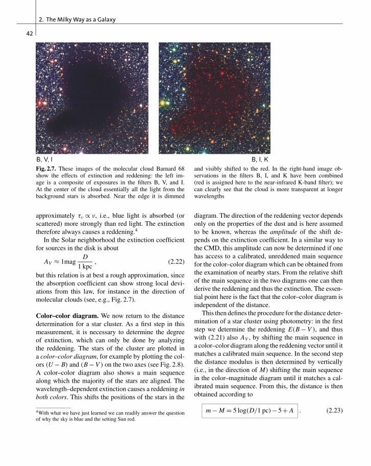
Fig. 2.7. These images of the molecular cloud Barnard 68show the effects of extinction and reddening: the left im-age is a composite of exposures in the filters B, V, and I.At the center of the cloud essentially all the light from thebackground stars is absorbed. Near the edge it is dimmed
and visibly shifted to the red. In the right-hand image ob-servations in the filters B, I, and K have been combined(red is assigned here to the near-infrared K-band filter); wecan clearly see that the cloud is more transparent at longerwavelengths
approximately τν ∝ ν, i.e., blue light is absorbed (orscattered) more strongly than red light. The extinctiontherefore always causes a reddening.4
In the Solar neighborhood the extinction coefficientfor sources in the disk is about
AV ≈ 1magD
1 kpc, (2.22)
but this relation is at best a rough approximation, sincethe absorption coefficient can show strong local devi-ations from this law, for instance in the direction ofmolecular clouds (see, e.g., Fig. 2.7).
Color–color diagram. We now return to the distancedetermination for a star cluster. As a first step in thismeasurement, it is necessary to determine the degreeof extinction, which can only be done by analyzingthe reddening. The stars of the cluster are plotted ina color–color diagram, for example by plotting the col-ors (U − B) and (B − V ) on the two axes (see Fig. 2.8).A color–color diagram also shows a main sequencealong which the majority of the stars are aligned. Thewavelength–dependent extinction causes a reddening inboth colors. This shifts the positions of the stars in the
4With what we have just learned we can readily answer the questionof why the sky is blue and the setting Sun red.
diagram. The direction of the reddening vector dependsonly on the properties of the dust and is here assumedto be known, whereas the amplitude of the shift de-pends on the extinction coefficient. In a similar way tothe CMD, this amplitude can now be determined if onehas access to a calibrated, unreddened main sequencefor the color–color diagram which can be obtained fromthe examination of nearby stars. From the relative shiftof the main sequence in the two diagrams one can thenderive the reddening and thus the extinction. The essen-tial point here is the fact that the color–color diagram isindependent of the distance.
This then defines the procedure for the distance deter-mination of a star cluster using photometry: in the firststep we determine the reddening E(B − V ), and thuswith (2.21) also AV , by shifting the main sequence ina color–color diagram along the reddening vector until itmatches a calibrated main sequence. In the second stepthe distance modulus is then determined by vertically(i.e., in the direction of M) shifting the main sequencein the color–magnitude diagram until it matches a cal-ibrated main sequence. From this, the distance is thenobtained according to
m − M = 5 log(D/1 pc)−5+ A . (2.23)

2.2 Determination of Distances Within Our Galaxy
43
Fig. 2.8. Color–color diagram for main-sequence stars. Spec-tral types and absolute magnitudes are specified. Black bodies(T/103 K) would be located along the upper line. Interstellarreddening shifts the measured stellar locations parallel to thereddening vector indicated by the arrow
2.2.5 Spectroscopic Distance
From the spectrum of a star, the spectral type as wellas the luminosity class can be determined. The formeris determined from the strength of various absorptionlines in the spectrum, while the latter is obtained fromthe width of the lines. From the line width the surfacegravity of the star can be derived, and from that its ra-dius (more precisely, M/R2). From the spectral type andthe luminosity class the position of the star in the HRDfollows unambiguously. By means of stellar evolutionmodels, the absolute magnitude MV can then be de-termined. Furthermore, the comparison of the observedcolor with that expected from theory yields the color ex-cess E(B − V ), and from that we obtain AV . With thisinformation we are then able to determine the distanceusing
V − AV − MV = 5 log (D/pc)−5 . (2.24)
2.2.6 Distances of Visual Binary Stars
Kepler’s third law for a two-body problem,
P2 = 4π2
G(m1 +m2)a3 , (2.25)
specifies the relation between the orbital period P ofa binary star, the masses mi of the two components,and the semimajor axis a of the ellipse. The latter isdefined by the distance vector between the two starsin the course of one period. This law can be used todetermine the distance to a visual binary star. For sucha system, the period P and the angular diameter 2θ
of the orbit are direct observables. If one additionallyknows the mass of the two stars, for instance from theirspectral classification, a can be determined according to(2.25), and from this the distance follows with D = a/θ.
2.2.7 Distances of Pulsating Stars
Several types of pulsating stars show periodic changes intheir brightnesses, where the period of a star is relatedto its mass, and thus to its luminosity. This period–luminosity (PL) relation is ideally suited for distancemeasurements: since the determination of the period isindependent of distance, one can obtain the luminositydirectly from the period. The distance is thus directly de-rived from the measured magnitude using (2.24), if theextinction can be determined from color measurements.
The existence of a relation between the luminosityand the pulsation period can be expected from simplephysical considerations. Pulsations are essentially ra-dial density waves inside a star that propagate with thespeed of sound, cs. Thus, one can expect that the pe-riod is comparable to the sound crossing time throughthe star, P ∼ R/cs. The speed of sound cs in a gas is ofthe same order of magnitude as the thermal velocity ofthe gas particles, so that kBT ∼ mpc2
s , where mp is theproton mass (and thus a characteristic mass of particlesin the stellar plasma) and kB is Boltzmann’s constant.According to the virial theorem, one expects that the

44
2. The Milky Way as a Galaxy
gravitational binding energy of the star is about twicethe kinetic (i.e., thermal) energy, so that for a proton
G Mmp
R∼ kBT .
Combining these relations, for the pulsation period weobtain
P ∼ R
cs∼ R
√mp√
kBT∼ R3/2
√G M
∝ ρ−1/2 , (2.26)
where ρ is the mean density of the star. This is a remark-able result – the pulsation period depends only on themean density. Furthermore, the stellar luminosity is re-lated to its mass by approximately L ∝ M3. If we nowconsider stars of equal effective temperature Teff (whereL ∝ R2T 4
eff), we find that
P ∝ R3/2
√M
∝ L7/12 , (2.27)
which is the relation between period and luminosity thatwe were aiming for.
One finds that a well-defined period–luminosityrelation exists for three types of pulsating stars:
• δ Cepheid stars (classical Cepheids). These are youngstars found in the disk population (close to the Gal-actic plane) and in young star clusters. Owing totheir position in or near the disk, extinction alwaysplays a role in the determination of their lumi-nosity. To minimize the effect of extinction it isparticularly useful to look at the period–luminosityrelation in the near-IR (e.g., in the K-band atλ ∼ 2.4 μm). Furthermore, the scatter around theperiod–luminosity relation is smaller for longerwavelengths of the applied filter, as is also shownin Fig. 2.9. The period–luminosity relation is alsosteeper for longer wavelengths, resulting in a moreaccurate determination of the absolute magnitude.
• W Virginis stars, also called Population II Cepheids(we will explain the term of stellar populations inSect. 2.3.2). These are low-mass, metal-poor starslocated in the halo of the Galaxy, in globular clusters,and near the Galactic center.
• RR Lyrae stars. These are likewise Population II starsand thus metal-poor. They are found in the halo, inglobular clusters, and in the Galactic bulge. Their ab-solute magnitudes are confined to a narrow interval,MV ∈ [0.5, 1.0], with a mean value of about 0.6. This
obviously makes them very good distance indicators.More precise predictions of their magnitudes are pos-sible with the following dependence on metallicityand period:
〈MK 〉 = − (2.0±0.3) log(P/1d)
+ (0.06±0.04)[Fe/H]−0.7±0.1 .
(2.28)
Metallicity. In the last equation, the metallicity of a starwas introduced, which needs to be defined. In astro-physics, all chemical elements heavier than helium arecalled metals. These elements, with the exception ofsome traces of lithium, were not produced in the earlyUniverse but rather later in the interior of stars. Themetallicity is thus also a measure of the chemical evolu-tion and enrichment of matter in a star or gas cloud. Foran element X, the metallicity index of a star is defined as
[X/H] ≡ log
(n(X)
n(H)
)∗− log
(n(X)
n(H)
)�
, (2.29)
thus it is the logarithm of the ratio of the fraction of Xrelative to hydrogen in the star and in the Sun, wheren is the number density of the species considered. Forexample, [Fe/H] = −1 means that iron has only a tenthof its Solar abundance. The metallicity Z is the totalmass fraction of all elements heavier than helium; theSun has Z ≈ 0.02, meaning that about 98% of the Solarmass are contributed by hydrogen and helium.
The period–luminosity relations are not only of sig-nificant importance for distance determination withinour Galaxy. They also play an important role in ex-tragalactic astronomy, since by far the most luminousof the three types of pulsating stars listed above, theCepheids, are also found and observed in other gal-axies; they therefore enable us to directly determinethe distances of other galaxies, which is essential formeasuring the Hubble constant. These aspects will bediscussed in detail in Sect. 3.6.
2.3 The Structure of the Galaxy
Roughly speaking, the Galaxy consists of the disk, thecentral bulge, and the Galactic halo – a roughly spherical

2.3 The Structure of the Galaxy
45
Fig. 2.9. Period–luminosity relation for Gal-actic Cepheids, measured in three differentfilters bands (B, V, and I, from top tobottom). The absolute magnitudes werecorrected for extinction by using colors.The period is given in days. Open andsolid circles denote data for those Cepheidsfor which distances were estimated us-ing different methods; the three objectsmarked by triangles have a variable pe-riod and are discarded in the derivationof the period–luminosity relation. The lat-ter is indicated by the solid line, with itsparametrisation specified in the plots. Thebroken lines indicate the uncertainty rangeof the period–luminosity relation. The slopeof the period–luminosity relation increasesif one moves to redder filters
distribution of stars and globular clusters that surroundsthe disk. The disk, whose stars form the visible bandof the Milky Way, contains spiral arms similar to thoseobserved in other galaxies. The Sun, together with itsplanets, orbits around the Galactic center on an approx-imately circular orbit. The distance R0 to the Galacticcenter is not very well known, as we will discuss later.To have a reference value, the International Astronom-
ical Union (IAU) officially defined the value of R0 in1985,
R0 = 8.5 kpc official value, IAU 1985 . (2.30)
More recent examinations have, however, found thatthe real value is slightly smaller, R0 ≈ 8.0 kpc. The di-ameter of the disk of stars, gas, and dust is ∼ 40 kpc.
46
2. The Milky Way as a Galaxy
A schematic depiction of our Galaxy is shown inFig. 1.3. Its most important structural parameters arelisted in Table 2.1.
2.3.1 The Galactic Disk: Distribution of Stars
By measuring the distances of stars in the Solar neigh-borhood one can determine the three-dimensional stellardistribution. From these investigations, one finds thatthere are different stellar components, as we will discussbelow. For each of them, the number density in the direc-tion perpendicular to the Galactic disk is approximatelydescribed by an exponential law,
n(z) ∝ exp
(−|z|
h
), (2.31)
where the scale-height h specifies the thickness of therespective component. One finds that h varies betweendifferent populations of stars, motivating the definitionof different components of the Galactic disk. In princi-ple, three components need to be distinguished: (1) Theyoung thin disk contains the largest fraction of gas anddust in the Galaxy, and in this region star formation isstill taking place today. The youngest stars are found inthe young thin disk, which has a scale-height of abouthytd ∼ 100 pc. (2) The old thin disk is thicker and hasa scale-height of about hotd ∼ 325 pc. (3) The thick diskhas a scale-height of hthick ∼ 1.5 kpc. The thick diskcontributes only about 2% to the total mass density in theGalactic plane at z = 0. This separation into three diskcomponents is rather coarse and can be further refinedif one uses a finer classification of stellar populations.
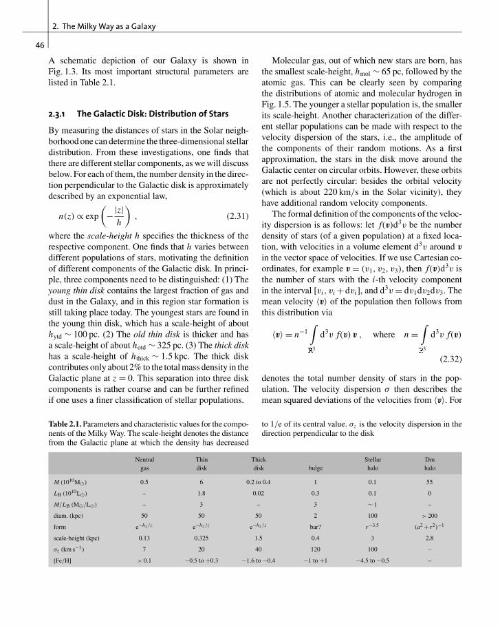
Table 2.1. Parameters and characteristic values for the compo-nents of the Milky Way. The scale-height denotes the distancefrom the Galactic plane at which the density has decreased
to 1/e of its central value. σz is the velocity dispersion in thedirection perpendicular to the disk
Neutral Thin Thick Stellar Dmgas disk disk bulge halo halo
M (1010M�) 0.5 6 0.2 to 0.4 1 0.1 55
LB (1010L�) – 1.8 0.02 0.3 0.1 0
M/LB (M�/L�) – 3 – 3 ∼ 1 –
diam. (kpc) 50 50 50 2 100 > 200
form e−hz/z e−hz/z e−hz/z bar? r−3.5 (a2 +r2)−1
scale-height (kpc) 0.13 0.325 1.5 0.4 3 2.8
σz (km s−1) 7 20 40 120 100 –
[Fe/H] > 0.1 −0.5 to +0.3 −1.6 to −0.4 −1 to +1 −4.5 to −0.5 –
Molecular gas, out of which new stars are born, hasthe smallest scale-height, hmol ∼ 65 pc, followed by theatomic gas. This can be clearly seen by comparingthe distributions of atomic and molecular hydrogen inFig. 1.5. The younger a stellar population is, the smallerits scale-height. Another characterization of the differ-ent stellar populations can be made with respect to thevelocity dispersion of the stars, i.e., the amplitude ofthe components of their random motions. As a firstapproximation, the stars in the disk move around theGalactic center on circular orbits. However, these orbitsare not perfectly circular: besides the orbital velocity(which is about 220 km/s in the Solar vicinity), theyhave additional random velocity components.
The formal definition of the components of the veloc-ity dispersion is as follows: let f(v)d3v be the numberdensity of stars (of a given population) at a fixed loca-tion, with velocities in a volume element d3v around v
in the vector space of velocities. If we use Cartesian co-ordinates, for example v = (v1, v2, v3), then f(v)d3v isthe number of stars with the i-th velocity componentin the interval [vi, vi +dvi], and d3v = dv1dv2dv3. Themean velocity 〈v〉 of the population then follows fromthis distribution via
〈v〉 = n−1∫R 3
d3v f(v) v , where n =∫R 3
d3v f(v)
(2.32)
denotes the total number density of stars in the pop-ulation. The velocity dispersion σ then describes themean squared deviations of the velocities from 〈v〉. For

2.3 The Structure of the Galaxy
47
a component i of the velocity vector, the dispersion σi
is defined as
σ2i = ⟨
(vi −〈vi〉)2⟩ = ⟨v2
i −〈vi〉2⟩= n−1
∫R 3
d3v f(v)(v2
i −〈vi〉2) . (2.33)
The larger σi is, the broader the distribution of thestochastic motions. We note that the same concept ap-plies to the velocity distribution of molecules in a gas.The mean velocity 〈v〉 at each point defines the bulkvelocity of the gas, e.g., the wind speed in the atmo-sphere, whereas the velocity dispersion is caused bythermal motion of the molecules and is determined bythe temperature of the gas.
The random motion of the stars in the directionperpendicular to the disk is the reason for the finitethickness of the population; it is similar to a thermaldistribution. Accordingly, it has the effect of a pressure,the so-called dynamical pressure of the distribution.This pressure determines the scale-height of the dis-tribution, which corresponds to the law of atmospheres.The larger the dynamical pressure, i.e., the larger thevelocity dispersion σz perpendicular to the disk, thelarger the scale-height h will be. The analysis of starsin the Solar neighborhood yields σz ∼ 16 km/s for starsyounger than ∼ 3 Gyr, corresponding to a scale-heightof h ∼ 250 pc, whereas stars older than ∼ 6 Gyr havea scale-height of ∼ 350 pc and a velocity dispersion ofσz ∼ 25 km/s.
The density distribution of the total star population,obtained from counts and distance determinations ofstars, is to a good approximation described by
n(R, z) = n0(e−|z|/hthin +0.02e−|z|/hthick
)e−R/h R ;
(2.34)
here, R and z are the cylinder coordinates introducedabove (see Sect. 2.1), with the origin at the Galacticcenter, and hthin ≈ hotd ≈ 325 pc is the scale-height ofthe thin disk. The distribution in the radial direction canalso be well described by an exponential law, wherehR ≈ 3.5 kpc denotes the scale-length of the Galacticdisk. The normalization of the distribution is determinedby the density n ≈ 0.2 stars/pc3 in the Solar neighbor-hood, for stars in the range of absolute magnitudes of4.5 ≤ MV ≤ 9.5. The distribution described by (2.34) is
not smooth at z = 0; it has a kink at this point and it istherefore unphysical. To get a smooth distribution whichfollows the exponential law for large z and is smooth inthe plane of the disk, the distribution is slightly modi-fied. As an example, for the luminosity density of theold thin disk (that is proportional to the number densityof the stars), we can write:
L(R, z) = L0e−R/h R
cosh2(z/hz), (2.35)
with hz = 2hthin and L0 ≈ 0.05L�/pc3. The Sun isa member of the young thin disk and is located abovethe plane of the disk, at z = 30 pc.
2.3.2 The Galactic Disk:Chemical Composition and Age
Stellar Populations. The chemical composition of starsin the thin and the thick disks differs: we observe theclear tendency that stars in the thin disk have a highermetallicity than those in the thick disk. In contrast, themetallicity of stars in the Galactic halo and in the bulgeis smaller. To paraphrase these trends, one distinguishesbetween stars of Population I (Pop I) which have a Solar-like metallicity (Z ∼ 0.02) and are mainly located inthe thin disk, and stars of Population II (Pop II) thatare metal-poor (Z ∼ 0.001) and predominantly foundin the thick disk, in the halo, and in the bulge. In reality,stars cover a wide range in Z, and the figures aboveare only characteristic values. For stellar populationsa somewhat finer separation was also introduced, suchas “extreme Population I”, “intermediate Population II”,and so on. The populations also differ in age (stars ofPop I are younger than those of Pop II), in scale-height(as mentioned above), and in the velocity dispersionperpendicular to the disk (σz is larger for Pop II starsthan for Pop I stars).
We shall now attempt to understand the origin ofthese different metallicities and their relation to thescale-height and to age. We start with a brief discus-sion of the phenomenon that is the main reason for themetal enrichment of the interstellar medium.
Metallicity and Supernovae. Supernovae (SNe) areexplosive events. Within a few days, a SN can reach
48
2. The Milky Way as a Galaxy
a luminosity of 109 L�, which is a considerable fractionof the total luminosity of a galaxy; after that the lumi-nosity decreases again with a time-scale of weeks. In theexplosion, a star is disrupted and (most of) the matter ofthe star is driven into the interstellar medium, enrichingit with metals that were produced in the course of stellarevolution or in the process of the supernova explosion.
Classification of Supernovae. Depending on theirspectral properties, SNe are divided into several classes.SNe of Type I do not show any Balmer lines of hydro-gen in their spectrum, in contrast to those of Type II.A further subdivision of Type I SNe is based on spec-tral properties: SNe Ia show strong emission of SiII λ
6150 Å whereas no SiII at all is visible in spectra ofType Ib,c. Our current understanding of the supernovaphenomenon differs from this spectral classification.5
Following various observational results and also the-oretical analyses, we are confident today that SNe Iaare a phenomenon which is intrinsically different fromthe other supernova types. For this interpretation, it isof particular importance that SNe Ia are found in alltypes of galaxies, whereas we observe SNe II and SNeIb,c only in spiral and irregular galaxies, and here onlyin those regions in which blue stars predominate. Aswe will see in Chap. 3, the stellar population in ellip-tical galaxies consists almost exclusively of old stars,while spirals also contain young stars. From this ob-servational fact it is concluded that the phenomenon ofSNe II and SNe Ib,c is linked to a young stellar popula-tion, whereas SNe Ia occur in older stellar populations.We shall discuss the two classes of supernovae next.
Core-Collapse Supernovae. SNe II and SNe Ib,c arethe final stages in the evolution of massive (� 8M�)stars. Inside these stars, ever heavier elements are gener-ated by fusion: once all the hydrogen is used up, heliumwill be burned, then carbon, oxygen, etc. This chaincomes to an end when the iron nucleus is reached, theatomic nucleus with the highest binding energy per nu-
5This notation scheme (Type Ia, Type II, and so on) is characteristic forphenomena that one wishes to classify upon discovery, but for whichno physical interpretation is available at that time. Other examples arethe spectral classes of stars, which are not named in alphabetical orderaccording to their mass on the main sequence, or the division of Seyfertgalaxies into Type 1 and Type 2. Once such a notation is established,it often becomes permanent even if a later physical understanding ofthe phenomenon suggests a more meaningful classification.
cleon. After this no more energy can be gained fromfusion to heavier elements so that the pressure, whichis normally balancing the gravitational force in the star,can no longer be maintained. The star will thus collapseunder its own gravity. This gravitational collapse willproceed until the innermost region reaches a densityabout three times the density of an atomic nucleus. Atthis point the so-called rebounce occurs: a shock waveruns towards the surface, thereby heating the infallingmaterial, and the star explodes. In the center, a compactobject probably remains – a neutron star or, possibly,depending on the mass of the iron core, a black hole.Such neutron stars are visible as pulsars6 at the locationof some historically observed SNe, the most famous ofwhich is the Crab pulsar which has been identified witha supernovae explosion seen by Chinese astronomers in1054. Presumably all neutron stars have been formed insuch core-collapse supernovae.
The major fraction of the binding energy releasedin the formation of the compact object is emitted inthe form of neutrinos: about 3×1053 erg. Undergroundneutrino detectors were able to trace about 10 neutrinosoriginating from SN 1987A in the Large MagellanicCloud. Due to the high density inside the star afterthe collapse, even neutrinos, despite their very smallcross-section, are absorbed and scattered, so that partof their outward-directed momentum contributes to theexplosion of the stellar envelope. This shell expands atv ∼ 10 000 km/s, corresponding to a kinetic energy ofEkin ∼ 1051 erg. Of this, only about 1049 erg is convertedinto photons in the hot envelope and then emitted – theenergy of a SN that is visible in photons is thus onlya small fraction of the total energy produced.
Owing to the various stages of nuclear fusion in theprogenitor star, the chemical elements are arranged inshells: the light elements (H, He) in the outer shells, andthe heavier elements (C, O, Ne, Mg, Si, Ar, Ca, Fe, Ni) inthe inner ones – see Fig. 2.10. The explosion ejects theminto the interstellar medium which is thus chemicallyenriched. It is important to note that mainly nuclei withan even number of protons and neutrons are formed.This is a consequence of the nuclear reaction chains6Pulsars are sources which show a very regular periodic radiation,most often seen at radio frequencies. Their periods lie in the rangefrom ∼ 10−3 s (millisecond pulsars) to ∼ 5 s. Their pulse period isidentified as the rotational period of the neutron star – an object withabout one Solar mass and a radius of ∼ 10 km. The matter density inneutron stars is about the same as that in atomic nuclei.

2.3 The Structure of the Galaxy
49
Fig. 2.10. Chemical shell structure of a mas-sive star at the end of its life. The elementsthat have been formed in the various stagesof the nuclear burning are ordered in a struc-ture resembling that of an onion. This is theinitial condition for a supernova explosion
involved, where successive nuclei in this chain are ob-tained by adding an α-particle (or 4He-nucleus), i.e.,two protons and two neutrons. Such elements are there-fore called α-elements. The dominance of α-elementsin the chemical abundance of the interstellar mediumis thus a clear indication of nuclear fusion occurring inthe He-rich zones of stars where the hydrogen has beenburnt.
Supernovae Type Ia. SNe Ia are most likely the ex-plosions of white dwarfs (WDs). These compact starswhich form the final evolutionary stages of less mas-sive stars no longer maintain their internal pressure bynuclear fusion. Rather, they are stabilized by the degen-eracy pressure of the electrons – a quantum mechanicalphenomenon. Such a white dwarf can only be stableif its mass does not exceed a limiting mass, the Chan-drasekhar mass; it has a value of MCh ≈ 1.44M�. ForM > MCh, the degeneracy pressure can no longer bal-ance the gravitational force. If matter falls onto a WDwith mass below MCh, as may happen by accretionin close binary systems, its mass will slowly increaseand approach the limiting mass. At about M ≈ 1.3M�,carbon burning will ignite in its interior, transformingabout half of the star into iron-group elements, i.e.,iron, cobalt, and nickel. The resulting explosion of thestar will enrich the ISM with ∼ 0.6M� of Fe, whilethe WD itself will be torn apart completely, leaving noremnant star.
Since the initial conditions are probably very homo-geneous for the class of SNe Ia (defined by the limitingmass prior to the trigger of the explosion), they are goodcandidates for standard candles: all SNe Ia have approx-imately the same luminosity. As we will discuss later(see Sect. 8.3.1), this is not really the case, but neverthe-less SNe Ia play an important role in the cosmological
distance determination, and thus in the determination ofcosmological parameters.
This interpretation of the different types of SNe ex-plains why one finds core-collapse SNe only in galaxiesin which star formation occurs. They are the final stagesof massive, i.e., young, stars which have a lifetime ofnot more than 2×10⁷ yr. By contrast, SNe Ia can occurin all types of galaxies.
In addition to SNe, metal enrichment of the interstel-lar medium (ISM) also takes place in other stages ofstellar evolution, by stellar winds or during phases inwhich stars eject part of their envelope which is thenvisible, e.g., as a planetary nebula. If the matter in thestar has been mixed by convection prior to such a phase,so that the metals newly formed by nuclear fusion in theinterior have been transported towards the surface of thestar, these metals will then be released into the ISM.
Age–Metallicity Relation. Assuming that at the begin-ning of its evolution the Milky Way had a chemicalcomposition with only low metal content, the metal-licity should be strongly related to the age of a stellarpopulation. With each new generation of stars, moremetals are produced and ejected into the ISM, partiallyby stellar winds, but mainly by SN explosions. Stars thatare formed later should therefore have a higher metalcontent than those that were formed in the early phaseof the Galaxy. One would therefore expect that a re-lation should exists between the age of a star and itsmetallicity.
For instance, under this assumption [Fe/H] can beused as an age indicator for a stellar population, with theiron predominantly being produced and ejected in SNeof type Ia. Therefore, newly formed stars have a higherfraction of iron when they are born than their prede-cessors, and the youngest stars should have the highest

50
2. The Milky Way as a Galaxy
iron abundance. Indeed one finds [Fe/H] = −4.5 forextremely old stars (i.e., 3×10⁻⁵ of the Solar iron abun-dance), whereas very young stars have [Fe/H] = 1, sotheir metallicity can significantly exceed that of the Sun.
However, this age–metallicity relation is not verytight. On the one hand, SNe Ia occur only � 109 yearsafter the formation of a stellar population. The exacttime-span is not known because even if one accepts thescenario for SN Ia described above, it is unclear in whatform and in what systems the accretion of material ontothe white dwarf takes place and how long it typicallytakes until the limiting mass is reached. On the otherhand, the mixing of the SN ejecta in the ISM occurs onlylocally, so that large inhomogeneities of the [Fe/H] ra-tio may be present in the ISM, and thus even for starsof the same age. An alternative measure for metallic-ity is [O/H], because oxygen, which is an α-element,is produced and ejected mainly in supernova explo-sions of massive stars. These begin only ∼ 107 yr afterthe formation of a stellar population, which is virtuallyinstantaneous.
Characteristic values for the metallicity are −0.5� [Fe/H]� 0.3 in the thin disk, while for the thick disk−1.0� [Fe/H]�−0.4 is typical. From this, one candeduce that stars in the thin disk must be significantlyyounger on average than those in the thick disk. Thisresult can now be interpreted using the age–metallicityrelation. Either star formation has started earlier, orceased earlier, in the thick disk than in the thin disk,or stars that originally belonged to the thin disk havemigrated into the thick disk. The second alternative isfavored for various reasons. It would be hard to under-stand why molecular gas, out of which stars are formed,was much more broadly distributed in earlier times thanit is today, where we find it well concentrated near theGalactic plane. In addition, the widening of an initiallynarrow stellar distribution in time is also expected. Thematter distribution in the disk is not homogeneous and,along their orbits around the Galactic center, stars expe-rience this inhomogeneous gravitational field caused byother stars, spiral arms, and massive molecular clouds.Stellar orbits are perturbed by such fluctuations, i.e.,they gain a random velocity component perpendicularto the disk from local inhomogeneities of the gravita-tional field. In other words, the velocity dispersion σz ofa stellar population grows in time, and the scale-heightof a population increases. In contrast to stars, the gas
keeps its narrow distribution around the Galactic planedue to internal friction.
This interpretation is, however, not unambiguous.Another scenario for the formation of the thick diskis also possible, where the stars of the thick disk wereformed outside the Milky Way and only became con-stituents of the disk later, through accretion of satellitegalaxies. This model is supported, among other reasons,by the fact that the rotational velocity of the thick diskaround the Galactic center is smaller by ∼ 50 km/s thanthat of the thin disk. In other spirals, in which a thickdisk component was found and kinematically analyzed,the discrepancy between the rotation curves of the thickand thin disks is sometimes even stronger. In one case,the thick disk has been observed to rotate around thecenter of the galaxy in the opposite direction to the gasdisk. In such a case, the aforementioned model of theevolution of the thick disk by kinematic heating of starswould definitely not apply.
Mass-to-Light Ratio. The total stellar mass of the thindisk is ∼ 6×10¹⁰ M�, to which ∼ 0.5×10¹⁰ M� in theform of dust and gas has to be added. The luminosity ofthe stars in the thin disk is L B ≈ 1.8×10¹⁰ L�. Together,this yields a mass-to-light ratio of
M
L B≈ 3
M�L�
in thin disk . (2.36)
The M/L ratio in the thick disk is higher. For this com-ponent, one has M ∼ 3×10⁹ M� and L B ≈ 2×10⁸ L�,so that M/L B ∼ 15 in Solar units. The thick disk thusdoes not play any significant role for the total massbudget of the Galactic disk, and even less for its totalluminosity. On the other hand, the thick disk is invalu-able for the diagnosis of the dynamical evolution of thedisk. If the Milky Way were to be observed from theoutside, one would find a M/L value for the disk ofabout 4 in Solar units; this is a characteristic value forspiral galaxies.
2.3.3 The Galactic Disk: Dust and Gas
The spiral structure of the Milky Way and other spiralgalaxies is delineated by very young objects like O- and
2.3 The Structure of the Galaxy
51
B-stars and HII regions.7 This is the reason why spi-ral arms appear blue. Obviously, star formation in ourMilky Way takes place mainly in the spiral arms. Here,the molecular clouds – gas clouds which are sufficientlydense and cool for molecules to form in large abun-dance – contract under their own gravity and form newstars. The spiral arms are much less prominent in redlight. Emission in the red is dominated by an older stel-lar population, and these old stars have had time to moveaway from the spiral arms. The Sun is located close to,but not in, a spiral arm – the so-called Orion arm.
Observing the gas in the Galaxy is made possiblemainly by the 21-cm line emission of HI (neutral atomichydrogen) and by the emission of CO, the second-mostabundant molecule after H2 (molecular hydrogen). H2
is a symmetric molecule and thus has no electric dipolemoment, which is the reason why it does not radiatestrongly. In most cases it is assumed that the ratio ofCO to H2 is a universal constant (called the “X-factor”).Under this assumption, the distribution of CO can beconverted into that of the molecular gas. The Milky Wayis optically thin at 21 cm, i.e., 21-cm radiation is notabsorbed along its path from the source to the observer.With radio-astronomical methods it is thus possible toobserve atomic gas throughout the entire Galaxy.
To examine the distribution of dust, two options areavailable. First, dust is detected by the extinction itcauses. This effect can be analyzed quantitatively, for in-stance by star counts or by investigating the reddening ofstars (an example of this can be seen in Fig. 2.7). Second,dust emits thermal radiation observable in the FIR partof the spectrum, which was mapped by several satellitessuch as IRAS and COBE. By combining the sky maps ofthese two satellites at different frequencies the Galacticdistribution of dust was determined. The dust tempera-ture varies in a relatively narrow range between ∼ 17 Kand ∼ 21 K, but even across this small range, the dustemission varies, for fixed column density, by a factor∼ 5 at a wavelength of 100 μm. Therefore, one needsto combine maps at different frequencies in order to de-termine column densities and temperatures. In addition,the zodiacal light caused by the reflection of solar radia-tion by dust inside our Solar system has to be subtracted
7HII regions are nearly spherical regions of fully ionized hydrogen(thus the name HII region) surrounding a young hot star which pho-toionizes the gas. They emit strong emission lines of which the Balmerlines of hydrogen are strongest.
before the Galactic FIR emission can be analyzed. Thisis possible with multifrequency data because of the dif-ferent spectral shapes. The resulting distribution of dustis displayed in Fig. 2.11. It shows the concentration ofdust around the Galactic plane, as well as large-scaleanisotropies at high Galactic latitudes. The dust mapshown here is routinely used for extinction correctionwhen observing extragalactic sources.
Besides a strong concentration towards the Galac-tic plane, gas and dust are preferentially found in spiralarms where they serve as raw material for star formation.Molecular hydrogen (H2) and dust are generally foundat 3 kpc� R� 8 kpc, within |z|� 90 pc of both sides ofthe Galactic plane. In contrast, the distribution of atomichydrogen (HI) is observed out to much larger distancesfrom the Galactic center (R � 25 kpc), with a scale-height of ∼ 160 pc inside the Solar orbit, R � R0. Atlarger distances from the Galactic center, R � 12 kpc,the scale-height increases substantially to ∼ 1 kpc. Thegaseous disk is warped at these large radii though theorigin of this warp is unclear. For example, it maybe caused by the gravitational field of the MagellanicClouds. The total mass in the two components of hydro-gen is about M(HI) ≈ 4×10⁹ M� and M(H2) ≈ 109 M�,respectively, i.e., the gas mass in our Galaxy is less than∼ 10% of the stellar mass. The density of the gas in theSolar neighborhood is about ρ(gas) ∼ 0.04M�/pc3.
2.3.4 Cosmic Rays
The Magnetic Field of the Galaxy. Like many othercosmic objects, the Milky Way has a magnetic field. Theproperties of this field can be analyzed using a varietyof methods and we list some of them in the following.
• Polarization of stellar light. The light of distant starsis partially polarized, with the degree of polarizationbeing strongly related to the extinction, or reddening,of the star. This hints at the polarization being linkedto the dust causing the extinction. The light scat-tered by dust particles is partially linearly polarized,with the direction of polarization depending on thealignment of the dust grains. If their orientation wererandom, the superposition of the scattered radiationfrom different dust particles would add up to a van-ishing net polarization. However, a net polarization

52
2. The Milky Way as a Galaxy
Fig. 2.11. Distribution of dust in the Galaxy, derived froma combination of IRAS and COBE sky maps. The northernGalactic sky in Galactic coordinates is displayed on the left,the southern on the right. We can clearly see the concentra-
tion of dust towards the Galactic plane, as well as regionswith a very low column density of dust; these regions in thesky are particularly well suited for very deep extragalacticobservations
is measured, so the orientation of dust particles can-not be random, rather it must be coherent on largescales. Such a coherent alignment is provided bya large-scale magnetic field, whereby the orientationof dust particles, measurable from the polarizationdirection, indicates the (projected) direction of themagnetic field.
• The Zeeman effect. The energy levels in an atomchange if the atom is placed in a magnetic field. Ofparticular importance in the present context is the factthat the 21-cm transition line of neutral hydrogen issplit in a magnetic field. Because the amplitude ofthe line split is proportional to the strength of themagnetic field, the field strength can be determinedfrom observations of this Zeeman effect.
• Synchrotron radiation. When relativistic electronsmove in a magnetic field they are subject to theLorentz force. The corresponding acceleration is per-pendicular both to the velocity vector of the particlesand to the magnetic field vector. As a result, the elec-trons follow a helical (i.e., corkscrew) track, which isa superposition of circular orbits perpendicular to thefield lines and a linear motion along the field. Sinceaccelerated charges emit electromagnetic radiation,this helical movement is the source of the so-calledsynchrotron radiation (which will be discussed in
more detail in Sect. 5.1.2). This radiation, which isobservable at radio frequencies, is linearly polarized,with the direction of the polarization depending onthe direction of the magnetic field.
• Faraday rotation. If polarized radiation passesthrough a magnetized plasma, the direction of thepolarization rotates. The rotation angle dependsquadratically on the wavelength of the radiation,
Δθ = RM λ2 . (2.37)
The rotation measure RM is the integral along theline-of-sight towards the source over the electrondensity and the component B‖ of the magnetic fieldin direction of the line-of-sight,
RM = 81rad
cm2
D∫0
d�
pc
ne
cm−3
B‖G
. (2.38)
The dependence of the rotation angle (2.37) on λ al-lows us to determine the rotation measure RM, andthus to estimate the product of electron density andmagnetic field. If the former is known, one imme-diately gets information about B. By measuring theRM for sources in different directions and at differ-ent distances the magnetic field of the Galaxy can bemapped.

2.3 The Structure of the Galaxy
53
From applying the methods discussed above, we knowthat a magnetic field exists in the disk of our Milky Way.This field has a strength of about 4×10⁻⁶ G and mainlyfollows the spiral arms.
Cosmic Rays. We obtain most of the information aboutour Universe from the electromagnetic radiation thatwe observe. However, we receive an additional radia-tion component, the energetic cosmic rays. They consistprimarily of electrically charged particles, mainly elec-trons and nuclei. In addition to the particle radiation thatis produced in energetic processes at the Solar surface,a much more energetic cosmic ray component exists thatcan only originate in sources outside the Solar system.
The energy spectrum of the cosmic rays is, toa good approximation, a power law: the flux of par-ticles with energy larger than E can be written asS(> E) ∝ E−q , with q ≈ 1.7. However, the slope ofthe spectrum changes slightly, but significantly, at someenergy scales: at E ∼ 1015 eV the spectrum becomessteeper, and at E � 1018 eV it flattens again.8 Measure-ments of the spectrum at these high energies are ratheruncertain, however, because of the strongly decreasingflux with increasing energy. This implies that only veryfew particles are detected.
Cosmic Ray Acceleration and Confinement. To ac-celerate particles to such high energies, highly energeticprocesses are necessary. For energies below 1015 eV,very convincing arguments suggest SN remnants asthe sites of the acceleration. The SN explosion drivesa shock front9 into the ISM with an initial velocity of∼ 10 000 km/s. Plasma processes in a shock front canaccelerate some particles to very high energies. Thetheory of this diffuse shock acceleration predicts that
8These energies should be compared with those reached in par-ticle accelerators: LEP at CERN reached ∼ 100 GeV = 1011 eV.Hence, cosmic accelerators are much more efficient than man-mademachines.9Shock fronts are surfaces in a gas flow where the parameters ofstate for the gas, such as pressure, density, and temperature, changediscontinuously. The standard example for a shock front is the bang inan explosion, where a spherical shock wave propagates outwards fromthe point of explosion. Another example is the sonic boom caused, forexample, by airplanes that move at a speed exceeding the velocity ofsound. Such shock fronts are solutions of the hydrodynamic equations.They occur frequently in astrophysics, e.g., in explosion phenomenasuch as supernovae or in rapid (i.e., supersonic) flows such as thosewe will discuss in the context of AGNs.
the resulting energy spectrum of the particles followsa power law, the slope of which depends only on thestrength of the shock (i.e., the ratio of the densities onboth sides of the shock front). This power law agreesvery well with the slope of the observed cosmic ray spec-trum, if additional propagation processes in the MilkyWay are taken into account. The presence of very en-ergetic electrons in SN remnants is observed directlyby their synchrotron emission, so that the slope of theproduced spectrum is also directly observable.
Accelerated particles then propagate through theGalaxy where, due to the magnetic field, they movealong complicated helical tracks. Therefore, the direc-tion from which a particle arrives at Earth cannot beidentified with the direction to its source of origin.The magnetic field is also the reason why particles donot leave the Milky Way along a straight path, but in-stead are stored for a long time (∼ 107 yr) before theyeventually diffuse out, an effect also called confinement.
The sources of the particles with energy between∼ 1015 eV and ∼ 1018 eV are likewise presumed to belocated inside our Milky Way, because the magneticfield is sufficiently strong to confine them in the Gal-axy. However, SN remnants are not likely sources forparticles at these energies; in fact, the origin of theserays is largely unknown. Particles with energies largerthan ∼ 1018 eV are probably of extragalactic origin. Theradius of the helical tracks in the magnetic field of theGalaxy, i.e., their Larmor radius, is larger than the ra-dius of the Milky Way itself, so they cannot be confined.Their origin is also unknown, but AGNs are the mostprobable source of these particles. Finally, one of thelargest puzzles of high-energy astrophysics is the ori-gin of cosmic rays with E � 1019 eV. The energy ofthese particles is so large that they are able to inter-act with the cosmic microwave background to producepions and other particles, losing much of their energyin this process. These particles cannot propagate muchfurther than ∼ 10 Mpc through the Universe before theylose most of their energy. This implies that their accel-eration sites should be located in the close vicinity ofthe Milky Way. Since the curvature of the orbits of suchhighly energetic particles is very small, it should, inprinciple, be possible to identify their origin: there arenot many AGNs within 10 Mpc that are promising can-didates for the origin of these ultra-high-energy cosmicrays. However, the observed number of these particles

54
2. The Milky Way as a Galaxy
is so small that no reliable information on these sourceshas thus far been obtained.
Energy Density. It is interesting to realize that the en-ergy densities of cosmic rays, the magnetic field, theturbulent energy of the ISM, and the electromagneticradiation of the stars are about the same – as if an equi-librium between these different components has beenestablished. Since these components interact with eachother – e.g., the turbulent motions of the ISM can am-plify the magnetic field, and vice versa, the magneticfield affects the velocity of the ISM and of cosmic rays –it is not improbable that these interaction processes canestablish an equipartition of the energy densities.
Gamma Radiation from the Milky Way. The MilkyWay emits γ -radiation, as can be seen in Fig. 1.5. Thereis diffuse γ -ray emission which can be traced back tothe cosmic rays in the Galaxy. When these energeticparticles collide with nuclei in the interstellar medium,radiation is released. This gives rise to a continuum ra-diation which closely follows a power-law spectrum,such that the observed flux Sν is ∝ ν−α, with α ∼ 2. Thequantitative analysis of the distribution of this emis-sion provides the most important information about thespatial distribution of cosmic rays in the Milky Way.
Gamma-Ray Lines. In addition to the continuum ra-diation, one also observes line radiation in γ -rays, atenergies below ∼ 10 MeV. The first detected and mostprominent line has an energy of 1.809 MeV and corre-sponds to a radioactive decay of the Al26 nucleus. Thespatial distribution of this emission is strongly concen-trated towards the Galactic disk and thus follows theyoung stellar population in the Milky Way. Since thelifetime of the Al26 nucleus is short (∼ 106 yr), it mustbe produced near the emission site, which then impliesthat it is produced by the young stellar population. Itis formed in hot stars and released to the interstellarmedium either through stellar winds or core-collapsesupernovae. Gamma lines from other radioactive nucleihave been detected as well.
Annihilation Radiation from the Galaxy. Further-more, line radiation with an energy of 511 keV has beendetected in the Galaxy. This line is produced when anelectron and a positron annihilate into two photons, each
with an energy corresponding to the rest-mass energy ofan electron, i.e., 511 keV.10 This annihilation radiationwas identified first in the 1970s. With the Integral satel-lite, its emission morphology has been mapped with anangular resolution of ∼ 3◦. The 511 keV line emissionis detected both from the Galactic disk and the bulge.The angular resolution is not sufficient to tell whetherthe annihilation line traces the young stellar popula-tion (i.e., the thin disk) or the older population in thethick disk. However, one can compare the distributionof the annihilation radiation with that of Al26 and otherradioactive species. In about 85% of all decays Al26
emits a positron. If this positron annihilates close to itsproduction site one can predict the expected annihila-tion radiation from the distribution of the 1.809 MeVline. In fact, the intensity and angular distribution ofthe 511 keV line from the disk is compatible with thisscenario for the generation of positrons.
The origin of the annihilation radiation from thebulge, which has a luminosity larger than that fromthe disk by a factor ∼ 5, is unknown. One needs to finda plausible source for the production of positrons inthe bulge. There is no unique answer to this problem atpresent, but Type Ia supernovae and energetic processesnear low-mass X-ray binaries are prime candidates forthis source.
2.3.5 The Galactic Bulge
The Galactic bulge is the central thickening of our Gal-axy. Figure 1.2 shows another spiral galaxy from itsside, with its bulge clearly visible. The characteristicscale-length of the bulge is ∼ 1 kpc. Owing to the strongextinction in the disk, the bulge is best observed in theIR, for instance with the IRAS and COBE satellites.The extinction to the Galactic Center in the visual isAV ∼ 28 mag. However, some lines-of-sight close to theGalactic center exist where AV is significantly smaller,so that observations in optical and near IR light are pos-sible, e.g., in Baade’s window, located about 4◦ belowthe Galactic center at � ∼ 1◦, for which AV ∼ 2 mag(also see Sect. 2.6).
From the observations by COBE, and also from Gal-actic microlensing experiments (see Sect. 2.5), we know10 In addition to the two-photon annihilation, there is also an annihila-tion channel in which three photons are produced; the correspondingradiation forms a continuum spectrum, i.e., no spectral lines.

2.3 The Structure of the Galaxy
55
that our bulge has the shape of a bar, with the major axispointing away from us by about 30◦. The scale-heightof the bulge is ∼ 400 pc, with an axis ratio of ∼ 0.6.
As is the case for the exponential profiles that de-scribe the light distribution in the disk, the functionalform of the brightness distribution in the bulge is alsosuggested from observations of other spiral galaxies.The profiles of their bulges, observed from the outside,are much better determined than in our Galaxy wherewe are located amid its stars.
The de Vaucouleurs Profile. The brightness profileof our bulge can be approximated by the de Vau-couleurs law which describes the surface brightness Ias a function of the distance R from the center,
log
(I(R)
Ie
)= −3.3307
[(R
Re
)1/4
−1
],
(2.39)
with I(R) being the measured surface brightness, e.g.,in [I] = L�/pc2. Re is the effective radius, defined suchthat half of the luminosity is emitted from within Re,
Re∫0
dR R I(R) = 1
2
∞∫0
dR R I(R) . (2.40)
This definition of Re also leads to the numerical fac-tor on the right-hand side of (2.39). As one can easilysee from (2.39), Ie = I(Re) is the surface brightnessat the effective radius. An alternative form of the deVaucouleurs law is
I(R) = Ie exp(−7.669
[(R/Re)
1/4 −1])
. (2.41)
Because of its mathematical form, it is also called an r1/4
law. The r1/4 law falls off significantly more slowly thanan exponential law for large R. For the Galactic bulge,one finds an effective radius of Re ≈ 0.7 kpc. With thede Vaucouleurs profile, a relation between luminosity,effective radius, and surface brightness is obtained byintegrating over the surface brightness,
L =∞∫
0
dR 2πR I(R) = 7.215πIe R2e . (2.42)
Stellar Age Distribution in the Bulge. The stars inthe bulge cover a large range in metallicity, −1 �[Fe/H]�+1, with a mean of about 0.3, i.e., the meanmetallicity is about twice that of the Sun. This highmetallicity hints at a contribution by a rather youngpopulation, whereas the color of the bulge stars pointstowards a predominantly old stellar population. Thebulge also contains about 108 M� in molecular gas. Onthe other hand, one finds very metal-poor RR Lyraestars, i.e., old stars. However, the distinction in mem-bership between bulge and disk stars is not easy, so itis possible that the young component may actually bepart of the inner disk.
The mass of the bulge is about Mbulge ∼ 1010 M� andits luminosity is L B,bulge ∼ 3×10⁹ L�, which results ina mass-to-light ratio of
M
L≈ 3
M�L�
in the bulge , (2.43)
very similar to that of the thin disk.
2.3.6 The Visible Halo
The visible halo of our Galaxy consists of about 150globular clusters and field stars with a high velocitycomponent perpendicular to the Galactic plane. A glob-ular cluster is a collection of typically several hundredthousand stars, contained within a spherical region of ra-dius ∼ 20 pc. The stars in the cluster are gravitationallybound and orbit in the common gravitational field. Theold globular clusters with [Fe/H] < −0.8 have an ap-proximately spherical distribution around the Galacticcenter. A second population of globular clusters existsthat contains younger stars with a higher metallicity,[Fe/H] > −0.8. They have a more oblate geometri-cal distribution and are possibly part of the thick diskbecause they show roughly the same scale-height.
Most globular clusters are at a distance of r � 35 kpc(with r = √
R2 + z2) from the Galactic center, but someare also found at r > 60 kpc. At these distances it is hardto judge whether these objects are part of the Galaxyor whether they have been captured from a neighboringgalaxy, such as the Magellanic Clouds. Also, field starshave been found at distances out to r ∼ 50 kpc, whichis the reason why one assumes a characteristic value ofrhalo ∼ 50 kpc for the extent of the visible halo.

56
2. The Milky Way as a Galaxy
The density distribution of metal-poor globularclusters and field stars in the halo is described by
n(r) ∝ r−3.5 . (2.44)
Alternatively, one can fit a de Vaucouleurs profile to thedensity distribution, which results in an effective radiusof re ∼ 2.7 kpc.
At large distances from the disk, neutral hydrogenis also found, in the form of clouds. Most of theseclouds, visible in 21-cm line emission, have a nega-tive radial velocity, i.e., they are moving towards us,with velocities of up to vr ∼ −400 km/s. These high-velocity clouds (HVCs) cannot be following the generalGalactic rotation. We have virtually no means of de-termining the distances of these clouds, and thus theirorigin and nature are still subject to discussion. There isone exception, however: the Magellanic Stream is a nar-row band of HI emission which follows the MagellanicClouds along their orbit around the Galaxy (also seeFig. 6.6). This gas stream may be the result of a closeencounter of the Magellanic Clouds with the Milky Wayin the past. The (tidal) gravitational force that the MilkyWay had imposed on our neighboring galaxies in suchan encounter could strip away part of the interstellar gasfrom them.
2.3.7 The Distance to the Galactic Center
As already mentioned, our distance from the Galacticcenter is rather difficult to measure and thus not veryprecisely known. The general problem with such a mea-surement is the high extinction in the disk, prohibitingmeasurements of the distance of individual stars closeto the Galactic center. Thus, one has to rely on moreindirect methods, and the most important ones will beoutlined here.
The visible halo of our Milky Way is populated byglobular clusters and also by field stars. They havea spherical, or, more generally, a spheroidal distribution.The center of this distribution is obviously the center ofgravity of the Milky Way, around which the halo objectsare moving. If one measures the three-dimensional dis-tribution of the halo population, the geometrical centerof this distribution should correspond to the Galacticcenter.
This method can indeed be applied because, due totheir extended distribution, halo objects can be observed
at relatively large Galactic latitudes where they are nottoo strongly affected by extinction. As was discussedin Sect. 2.2, the distance determination of globular clus-ters is possible using photometric methods. On the otherhand, one also finds RR Lyrae stars in globular clustersto which the period–luminosity relation can be applied.Therefore, the spatial distribution of the globular clus-ters can be determined. However, at about 150, thenumber of known globular clusters is relatively small,resulting in a fairly large statistical error for the deter-mination of the common center. Much more numerousare the RR Lyrae field stars in the halo, for which dis-tances can be measured using the period–luminosityrelation. The statistical error in determining the cen-ter of their distribution is therefore much smaller. Onthe other hand, this distance to the Galactic center isbased only on the calibration of the period–luminosityrelation, and any uncertainty in this will propagate intoa systematic error on R0. Effects of the extinction addto this. However, such effects can be minimized by ob-serving the RR Lyrae stars in the NIR, which in additionbenefits from the narrower luminosity distribution of RRLyrae stars in this wavelength regime. These analysesyield a value of R0 ≈ 8.0 kpc (see Fig. 2.12).
Fig. 2.12. The number of RR Lyrae stars as a function of dis-tance, measured in a direction that closely passes the Galacticcenter, at � = 0◦ and b = −8◦. If we assume a sphericallysymmetric distribution of the RR Lyrae stars, concentrated to-wards the center, the distance to the Galactic center can beidentified with the maximum of this distribution
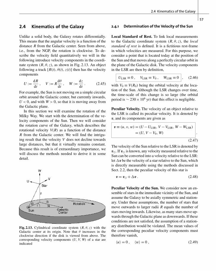
2.4 Kinematics of the Galaxy
57
2.4 Kinematics of the Galaxy
Unlike a solid body, the Galaxy rotates differentially.This means that the angular velocity is a function of thedistance R from the Galactic center. Seen from above,i.e., from the NGP, the rotation is clockwise. To de-scribe the velocity field quantitatively we will in thefollowing introduce velocity components in the coordi-nate system (R, θ, z), as shown in Fig. 2.13. An objectfollowing a track [R(t), θ(t), z(t)] then has the velocitycomponents
U := dR
dt, V := R
dθ
dt, W := dz
dt. (2.45)
For example, the Sun is not moving on a simple circularorbit around the Galactic center, but currently inwards,U < 0, and with W > 0, so that it is moving away fromthe Galactic plane.
In this section we will examine the rotation of theMilky Way. We start with the determination of the ve-locity components of the Sun. Then we will considerthe rotation curve of the Galaxy, which describes therotational velocity V(R) as a function of the distanceR from the Galactic center. We will find the intrigu-ing result that the velocity V does not decline towardslarge distances, but that it virtually remains constant.Because this result is of extraordinary importance, wewill discuss the methods needed to derive it in somedetail.
Fig. 2.13. Cylindrical coordinate system (R, θ, z) with theGalactic center at its origin. Note that θ increases in theclockwise direction if the disk is viewed from above. Thecorresponding velocity components (U, V, W) of a star areindicated
2.4.1 Determination of the Velocity of the Sun
Local Standard of Rest. To link local measurementsto the Galactic coordinate system (R, θ, z), the localstandard of rest is defined. It is a fictitious rest-framein which velocities are measured. For this purpose, weconsider a point that is located today at the position ofthe Sun and that moves along a perfectly circular orbit inthe plane of the Galactic disk. The velocity componentsin the LSR are then by definition,
ULSR ≡ 0 , VLSR ≡ V0 , WLSR ≡ 0 , (2.46)
with V0 ≡ V(R0) being the orbital velocity at the loca-tion of the Sun. Although the LSR changes over time,the time-scale of this change is so large (the orbitalperiod is ∼ 230×106 yr) that this effect is negligible.
Peculiar Velocity. The velocity of an object relative tothe LSR is called its peculiar velocity. It is denoted byv, and its components are given as
v ≡ (u, v,w) = (U −ULSR, V − VLSR, W − WLSR)
= (U, V − V0, W) .
(2.47)
The velocity of the Sun relative to the LSR is denoted byv�. If v� is known, any velocity measured relative to theSun can be converted into a velocity relative to the LSR:let Δv be the velocity of a star relative to the Sun, whichis directly measurable using the methods discussed inSect. 2.2, then the peculiar velocity of this star is
v = v� +Δv . (2.48)
Peculiar Velocity of the Sun. We consider now an en-semble of stars in the immediate vicinity of the Sun, andassume the Galaxy to be axially symmetric and station-ary. Under these assumptions, the number of stars thatmove outwards to larger radii R equals the number ofstars moving inwards. Likewise, as many stars move up-wards through the Galactic plane as downwards. If theseconditions are not satisfied, the assumption of a station-ary distribution would be violated. The mean values ofthe corresponding peculiar velocity components musttherefore vanish,
〈u〉 = 0 , 〈w〉 = 0 , (2.49)

58
2. The Milky Way as a Galaxy
where the brackets denote an average over the ensembleconsidered. The analog argument is not valid for the v
component because the mean value of v depends on thedistribution of the orbits: if only circular orbits in thedisk existed, we would also have 〈v〉 = 0 (this is trivial,since then all stars would have v = 0), but this is notthe case. From a statistical consideration of the orbits inthe framework of stellar dynamics, one deduces that 〈v〉is closely linked to the radial velocity dispersion of thestars: the larger it is, the more 〈v〉 deviates from zero.One finds that
〈v〉 = −C⟨u2⟩ , (2.50)
where C is a positive constant that depends on the den-sity distribution and on the local velocity distributionof the stars. The sign in (2.50) follows from noting thata circular orbit has a higher tangential velocity than el-liptical orbits, which in addition have a non-zero radialcomponent. Equation (2.50) expresses the fact that themean rotational velocity of a stellar population aroundthe Galactic center deviates from the corresponding cir-cular orbit velocity, and that the deviation is stronger fora larger radial velocity dispersion. This phenomenon isalso known as asymmetric drift. From the mean of (2.48)over the ensemble considered and by using (2.49) and(2.50), one obtains
v� = (−〈Δu〉 ,−C⟨u2⟩−〈Δv〉 ,−〈Δw〉) .
(2.51)
One still needs to determine the constant C in orderto make use of this relation. This is done by consider-ing different stellar populations and measuring
⟨u2
⟩and
〈Δv〉 separately for each of them. If these two quanti-ties are then plotted in a diagram (see Fig. 2.14), a linearrelation is obtained, as expected from (2.50). The slopeC can be determined directly from this diagram. Fur-thermore, from the intersection with the 〈Δv〉-axis, v�is readily read off. The other velocity components in(2.51) follow by simply averaging, yielding the result:
v� = (−10, 5, 7) km/s . (2.52)
Hence, the Sun is currently moving inwards, upwards,and faster than it would on a circular orbit at its location.We have therefore determined v�, so we are now ableto analyze any measured stellar velocities relative to the
LSR. However, we have not yet discussed how V0, therotational velocity of the LSR itself, is determined.
Velocity Dispersion of Stars. The dispersion of the stel-lar velocities relative to the LSR can now be determined,i.e., the mean square deviation of their velocities fromthe velocity of the LSR. For young stars (A stars, forexample), this dispersion happens to be small. For olderK giants it is larger, and is larger still for old, metal-poor red dwarf stars. We observe a very well-definedvelocity-metallicity relation. When this is combinedwith the age–metallicity relation it appears that theoldest stars have the highest peculiar velocities. Thiseffect is observed in all three coordinates. This re-sult is in agreement with the relation between the ageof a stellar population and its scale-height (discussedin Sect. 2.3.1), the latter being linked to the velocitydispersion via σz .
Asymmetric Drift. If one considers high-velocity stars,only a few are found that have v > 65 km/s and whichare thus moving much faster around the Galactic centerthan the LSR. However, quite a few stars are found thathave v < −250 km/s, so their orbital velocity is oppo-site to the direction of rotation of the LSR. Plotted ina (u −v)-diagram, a distribution is found which is nar-rowly concentrated around u = 0 km/s = v for youngstars, as already mentioned above, and which gets in-creasingly wider for older stars. For the oldest stars,
Fig. 2.14. The velocity components 〈Δv〉 = 〈v〉−v� are plot-ted against
⟨u2
⟩for stars in the Solar neighborhood. Because
of the linear relation, v� can be read off from the intersectionwith the x-axis, and C from the slope

2.4 Kinematics of the Galaxy
59
which belong to the halo population, one obtains a cir-cular envelope with its center located at u = 0 km/s andv ≈ −220 km/s (see Fig. 2.15). If we assume that theGalactic halo, to which these high-velocity stars belong,does not rotate (or only very slowly), this asymmetry inthe v-distribution can only be caused by the rotation ofthe LSR. The center of the envelope then has to be at−V0. This yields the orbital velocity of the LSR
V0 ≡ V(R0) = 220 km/s . (2.53)
Knowing this velocity, we can then compute the massof the Galaxy inside the Solar orbit. A circular orbitis characterized by an equilibrium between centrifugaland gravitational acceleration, V 2/R = G M(< R)/R2,so that
M(< R0) = V 20 R0
G= 8.8×10¹⁰ M� . (2.54)
Furthermore, for the orbital period of the LSR, which issimilar to that of the Sun, one obtains
P = 2πR0
V0= 230×106 yr . (2.55)
Hence, during the lifetime of the Solar System, esti-mated to be ∼ 4.6×10⁹ yr, it has completed about 20orbits around the Galactic center.
Fig. 2.15. The motion of the Sun around theGalactic center is reflected in the asymmetricdrift: while young stars in the Solar vicinityhave velocities very similar to the Solar ve-locity, i.e., small relative velocities, membersof other populations (and of other Milky Waycomponents) have different velocities – e.g.,for halo objects v = −220 km/s on average.Thus, different velocity ellipses show up in a(u −v)-diagram
2.4.2 The Rotation Curve of the Galaxy
From observations of the velocity of stars or gas aroundthe Galactic center, the rotational velocity V can bedetermined as a function of the distance R from theGalactic center. In this section, we will describe methodsto determine this rotation curve and discuss the result.
We consider an object at distance R from the Galacticcenter which moves along a circular orbit in the Galacticplane, has a distance D from the Sun, and is located ata Galactic longitude � (see Fig. 2.16). In a Cartesiancoordinate system with the Galactic center at the origin,the positional and velocity vectors (we only considerthe two components in the Galactic plane because weassume a motion in the plane) are given by
r = R
(sin θ
cos θ
), V = r = V(R)
(cos θ
− sin θ
),
where θ denotes the angle between the Sun and the ob-ject as seen from the Galactic center. From the geometryshown in Fig. 2.16 it follows that
r =(
D sin �
R0 − D cos �
).
If we now identify the two expressions for the com-ponents of r, we obtain
sin θ = (D/R) sin � ,
cos θ = (R0/R)− (D/R) cos � .
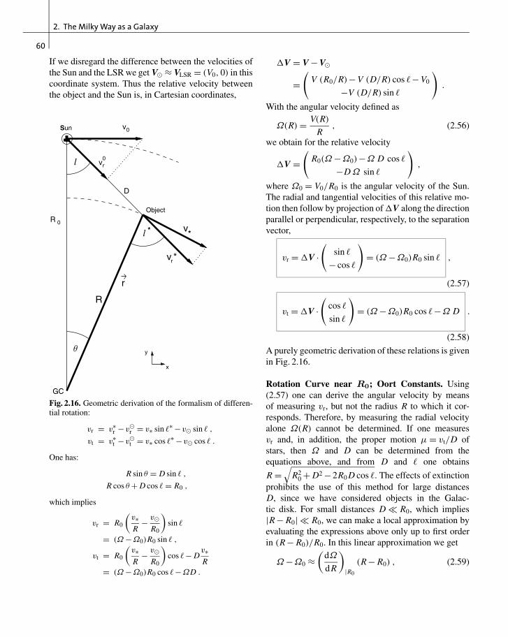
60
2. The Milky Way as a Galaxy
If we disregard the difference between the velocities ofthe Sun and the LSR we get V� ≈ VLSR = (V0, 0) in thiscoordinate system. Thus the relative velocity betweenthe object and the Sun is, in Cartesian coordinates,
Fig. 2.16. Geometric derivation of the formalism of differen-tial rotation:
vr = v∗r −v�
r = v∗ sin �∗ −v� sin � ,
vt = v∗t −v�
t = v∗ cos �∗ −v� cos � .
One has:
R sin θ = D sin � ,
R cos θ + D cos � = R0 ,
which implies
vr = R0
(v∗R
− v�R0
)sin �
= (Ω −Ω0)R0 sin � ,
vt = R0
(v∗R
− v�R0
)cos �− D
v∗R
= (Ω −Ω0)R0 cos �−ΩD .
ΔV = V − V�
=(
V (R0/R)− V (D/R) cos �− V0
−V (D/R) sin �
).
With the angular velocity defined as
Ω(R) = V(R)
R, (2.56)
we obtain for the relative velocity
ΔV =(
R0(Ω −Ω0)−Ω D cos �
−D Ω sin �
),
where Ω0 = V0/R0 is the angular velocity of the Sun.The radial and tangential velocities of this relative mo-tion then follow by projection of ΔV along the directionparallel or perpendicular, respectively, to the separationvector,
vr = ΔV ·(
sin �
− cos �
)= (Ω −Ω0)R0 sin � ,
(2.57)
vt = ΔV ·(
cos �
sin �
)= (Ω −Ω0)R0 cos �−Ω D .
(2.58)
A purely geometric derivation of these relations is givenin Fig. 2.16.
Rotation Curve near R0; Oort Constants. Using(2.57) one can derive the angular velocity by meansof measuring vr, but not the radius R to which it cor-responds. Therefore, by measuring the radial velocityalone Ω(R) cannot be determined. If one measuresvr and, in addition, the proper motion μ = vt/D ofstars, then Ω and D can be determined from theequations above, and from D and � one obtains
R =√
R20 + D2 −2R0 D cos �. The effects of extinction
prohibits the use of this method for large distancesD, since we have considered objects in the Galac-tic disk. For small distances D R0, which implies|R − R0| R0, we can make a local approximation byevaluating the expressions above only up to first orderin (R − R0)/R0. In this linear approximation we get
Ω −Ω0 ≈(
dΩ
dR
)|R0
(R − R0) , (2.59)

2.4 Kinematics of the Galaxy
61
where the derivative has to be evaluated at R = R0.Hence
vr = (R − R0)
(dΩ
dR
)|R0
R0 sin � ,
and furthermore, with (2.56),
R0
(dΩ
dR
)|R0
= R0
R
[(dV
dR
)|R0
− V
R
]
≈(
dV
dR
)|R0
− V0
R0,
in zeroth order in (R − R0)/R0. Combining the last twoequations yields
vr =[(
dV
dR
)|R0
− V0
R0
](R − R0) sin � ; (2.60)
in analogy to this, we obtain for the tangential velocity
vt =[(
dV
dR
)|R0
− V0
R0
](R − R0) cos �−Ω0 D .
(2.61)
For |R − R0| R0 it follows that R0 − R ≈ D cos �; ifwe insert this into (2.60) and (2.61) we get
vr ≈ A D sin 2� , vt ≈ A D cos 2�+ B D ,
(2.62)
where A and B are the Oort constants
A := −1
2
[(dV
dR
)|R0
− V0
R0
],
B := −1
2
[(dV
dR
)|R0
+ V0
R0
]. (2.63)
The radial and tangential velocity fields relative to theSun show a sine curve with period π, where vt and vr
are phase-shifted by π/4. This behavior of the velocityfield in the Solar neighborhood is indeed observed (seeFig. 2.17). By fitting the data for vr(�) and vt(�) for starsof equal distance D one can determine A and B, andthus
Ω0 = V0
R0= A − B,
(dV
dR
)|R0
= −(A + B) .
(2.64)
Fig. 2.17. The radial velocity vr of stars at a fixed distanceD is proportional to sin 2�; the tangential velocity vt is a lin-ear function of cos 2�. From the amplitude of the oscillatingcurves and from the mean value of vt the Oort constants Aand B can be derived, respectively (see (2.62))
The Oort constants thus yield the angular velocity ofthe Solar orbit and its derivative, and therefore thelocal kinematical information. If our Galaxy was ro-tating rigidly so that Ω was independent of the radius,A = 0 would follow. But the Milky Way rotates differ-entially, i.e., the angular velocity depends on the radius.Measurements yield the following values for A and B,
A = (14.8±0.8) km s−1 kpc−1 ,
B = (−12.4±0.6) km s−1 kpc−1 . (2.65)
Galactic Rotation Curve forR<R0; Tangent PointMethod. To measure the rotation curve for radii that aresignificantly smaller than R0, one has to turn to largewavelengths due to extinction in the disk. Usually the21-cm emission line of neutral hydrogen is used, whichcan be observed over large distances, or the emission ofCO in molecular gas. These gas components are foundthroughout the disk and are strongly concentrated to-wards the plane. Furthermore, the radial velocity caneasily be measured from the Doppler effect. However,since the distance to a hydrogen cloud cannot be deter-mined directly, a method is needed to link the measuredradial velocities to the distance of the gas from the Gal-actic center. For this purpose the tangent point methodis used.

62
2. The Milky Way as a Galaxy
Consider a line-of-sight at fixed Galactic longitude �,with cos � > 0 (thus “inwards”). The radial velocity vr
along this line-of-sight for objects moving on circu-lar orbits is a function of the distance D, according to(2.57). If Ω(R) is a monotonically decreasing function,vr attains a maximum where the line-of-sight is tangentto the local orbit, and thus its distance R from the Gal-actic center attains the minimum value Rmin. This is thecase at
D = R0 cos �, Rmin = R0 sin � (2.66)
(see Fig. 2.18). The maximum radial velocity there,according to (2.57), is
vr,max = [Ω(Rmin)−Ω0] R0 sin �
= V(Rmin)− V0 sin � , (2.67)
so that from the measured value of vr,max as a func-tion of direction �, the rotation curve inside R0 can bedetermined,
V(R) =(
R
R0
)V0 +vr,max(sin � = R/R0) . (2.68)
In the optical regime of the spectrum this methodcan only be applied locally, i.e., for small D, due toextinction. This is the case if one observes in a direc-tion nearly tangential to the orbit of the Sun, i.e., if
Fig. 2.18. The ISM is optically thin for21-cm radiation, and thus we receive the21-cm emission of HI regions from every-where in the Galaxy. Due to the motion ofan HI cloud relative to us, the wavelengthis shifted. This can be used to measurethe radial velocity of the cloud. With theassumption that the gas is moving on a cir-cular orbit around the Galactic center, oneexpects that for the cloud in the tangentpoint (cloud 4), the full velocity is pro-jected along the line-of-sight so that thiscloud will therefore have the largest radialvelocity. If the distance of the Sun to theGalactic center is known, the velocity ofa cloud and its distance from the Galacticcenter can then be determined
0 < π/2−� 1 or 0 < �−3π/2 1, or | sin �| ≈ 1,so that R0 − Rmin R0. In this case we get, to firstorder in (R0 − Rmin), using (2.66),
V(Rmin) ≈ V0 +(
dV
dR
)|R0
(Rmin − R0)
= V0 −(
dV
dR
)|R0
R0 (1− sin �) , (2.69)
so that with (2.67)
vr,max =[
V0 −(
dV
dR
)|R0
R0
](1− sin �)
= 2 A R0 (1− sin �) , (2.70)
where (2.63) was used in the last step. This relation canalso be used for determining the Oort constant A.
To determine V(R) for smaller R by employing thetangent point method, we have to observe in wavelengthregimes in which the Galactic plane is transparent, us-ing radio emission lines of gas. In Fig. 2.18, a typicalintensity profile of the 21-cm line along a line-of-sight is sketched; according to the Doppler effect thiscan be converted directly into a velocity profile us-ing vr = (λ−λ0)/λ0. It consists of several maxima thatoriginate in individual gas clouds. The radial velocity ofeach cloud is defined by its distance R from the Galactic
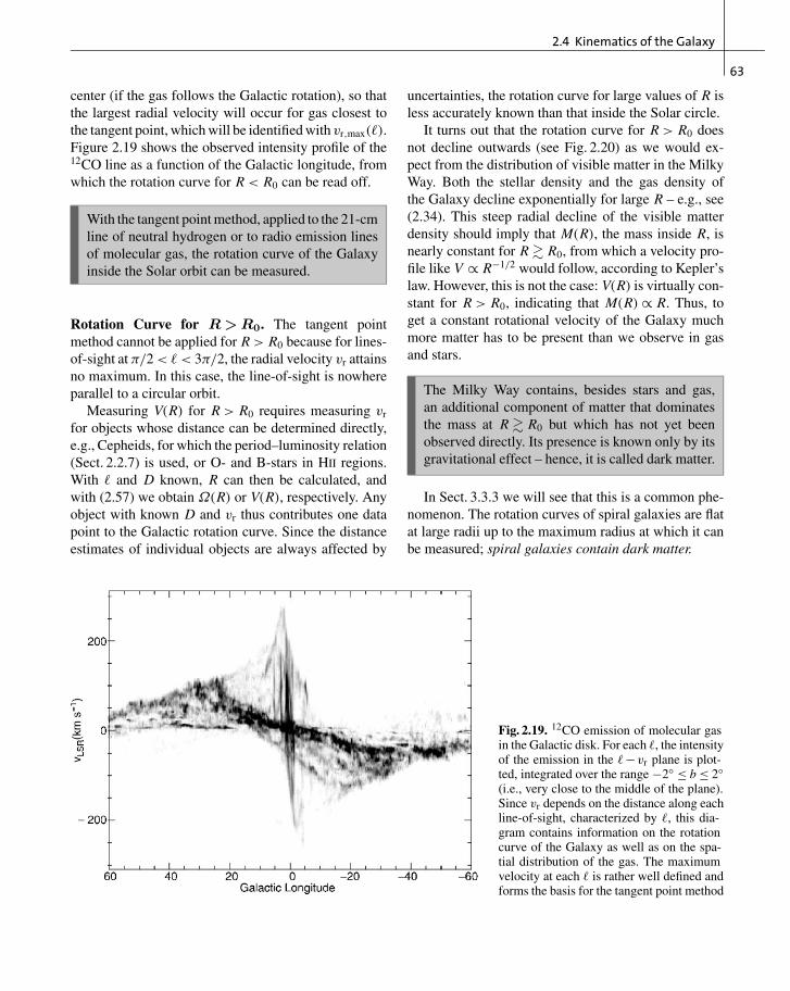
2.4 Kinematics of the Galaxy
63
center (if the gas follows the Galactic rotation), so thatthe largest radial velocity will occur for gas closest tothe tangent point, which will be identified with vr,max(�).Figure 2.19 shows the observed intensity profile of the12CO line as a function of the Galactic longitude, fromwhich the rotation curve for R < R0 can be read off.
With the tangent point method, applied to the 21-cmline of neutral hydrogen or to radio emission linesof molecular gas, the rotation curve of the Galaxyinside the Solar orbit can be measured.
Rotation Curve for R>R0. The tangent pointmethod cannot be applied for R > R0 because for lines-of-sight at π/2 < � < 3π/2, the radial velocity vr attainsno maximum. In this case, the line-of-sight is nowhereparallel to a circular orbit.
Measuring V(R) for R > R0 requires measuring vr
for objects whose distance can be determined directly,e.g., Cepheids, for which the period–luminosity relation(Sect. 2.2.7) is used, or O- and B-stars in HII regions.With � and D known, R can then be calculated, andwith (2.57) we obtain Ω(R) or V(R), respectively. Anyobject with known D and vr thus contributes one datapoint to the Galactic rotation curve. Since the distanceestimates of individual objects are always affected by
Fig. 2.19. 12CO emission of molecular gasin the Galactic disk. For each �, the intensityof the emission in the �−vr plane is plot-ted, integrated over the range −2◦ ≤ b ≤ 2◦(i.e., very close to the middle of the plane).Since vr depends on the distance along eachline-of-sight, characterized by �, this dia-gram contains information on the rotationcurve of the Galaxy as well as on the spa-tial distribution of the gas. The maximumvelocity at each � is rather well defined andforms the basis for the tangent point method
uncertainties, the rotation curve for large values of R isless accurately known than that inside the Solar circle.
It turns out that the rotation curve for R > R0 doesnot decline outwards (see Fig. 2.20) as we would ex-pect from the distribution of visible matter in the MilkyWay. Both the stellar density and the gas density ofthe Galaxy decline exponentially for large R – e.g., see(2.34). This steep radial decline of the visible matterdensity should imply that M(R), the mass inside R, isnearly constant for R � R0, from which a velocity pro-file like V ∝ R−1/2 would follow, according to Kepler’slaw. However, this is not the case: V(R) is virtually con-stant for R > R0, indicating that M(R) ∝ R. Thus, toget a constant rotational velocity of the Galaxy muchmore matter has to be present than we observe in gasand stars.
The Milky Way contains, besides stars and gas,an additional component of matter that dominatesthe mass at R � R0 but which has not yet beenobserved directly. Its presence is known only by itsgravitational effect – hence, it is called dark matter.
In Sect. 3.3.3 we will see that this is a common phe-nomenon. The rotation curves of spiral galaxies are flatat large radii up to the maximum radius at which it canbe measured; spiral galaxies contain dark matter.

64
2. The Milky Way as a Galaxy
Fig. 2.20. Rotation curve of the MilkyWay. Inside the “Solar circle”, that is atR < R0, the radial velocity is determinedquite accurately using the tangent pointmethod; the measurements outside havelarger uncertainties
The nature of dark matter is thus far unknown; inprinciple, we can distinguish two totally different kindsof dark matter candidates:• Astrophysical dark matter, consisting of compact
objects – e.g., faint stars like white dwarfs, browndwarfs, black holes, etc. Such objects were assignedthe name MACHOs, which stands for “MAssiveCompact Halo Objects”.
• Particle physics dark matter, consisting of elemen-tary particles which have thus far escaped detectionin accelerator laboratories.
Although the origin of astrophysical dark matter wouldbe difficult to understand (not least because of thebaryon abundance in the Universe – see Sect. 4.4.4 – andbecause of the metal abundance in the ISM), a directdistinction between the two alternatives through ob-servation would be of great interest. In the followingsection we will describe a method which is able toprobe whether the dark matter in our Galaxy consists ofMACHOs.
2.5 The Galactic Microlensing Effect:The Quest for CompactDark Matter
In 1986, Bohdan Paczynski proposed to test the possi-ble presence of MACHOs by performing microlensingexperiments. As we will soon see, this was a daring idea
at that time, but since then such experiments have beencarried out. In this section we will mainly summarizeand discuss the results of these searches for MACHOs.We will start with a description of the microlensing ef-fect and then proceed with its specific application to thesearch for MACHOs.
2.5.1 The Gravitational Lensing Effect I
Einstein’s Deflection Angle. Light, just like massiveparticles, is deflected in a gravitational field. This is oneof the specific predictions by Einstein’s theory of grav-ity, General Relativity. Quantitatively it predicts thata light beam which passes a point mass M at a distanceξ is deflected by an angle α, which amounts to
α = 4 G M
c2 ξ. (2.71)
The deflection law (2.71) is valid as long as α 1,which is the case for weak gravitational fields. If wenow set M = M�, R = R� in the foregoing equation,we obtain
α� ≈ 1′′. 74
for the light deflection at the limb of the Sun. This de-flection of light was measured during a Solar eclipse in1919 from the shift of the apparent positions of stars

2.5 The Galactic Microlensing Effect: The Quest for Compact Dark Matter
65
close to the shaded Solar disk. Its agreement with thevalue predicted by Einstein made him world-famousover night, because this was the first real and challeng-ing test of General Relativity. Although the precisionof the measured value back then was only ∼ 30%, itwas sufficient to confirm Einstein’s theory. By now thelaw (2.71) has been measured in the Solar System witha precision of about 0.1%, and Einstein’s prediction hasbeen confirmed.
Not long after the discovery of gravitational lightdeflection at the Sun, the following scenario was con-sidered. If the deflection of the light were sufficientlystrong, light from a very distant source could be vis-ible at two positions in the sky: one light ray couldpass a mass concentration, located between us and thesource, “to the right”, and the second one “to the left”, assketched in Fig. 2.21. The astrophysical consequence ofthis gravitational light deflection is also called the grav-itational lens effect. We will discuss various aspects of
Fig. 2.21. Sketch of a gravitational lens system. If a sufficientlymassive mass concentration is located between us and a distantsource, it may happen that we observe this source at twodifferent positions on the sphere
the lens effect in the course of this book, and we willreview its astrophysical applications.
The Sun is not able to cause multiple images of dis-tant sources. The maximum deflection angle α� is muchsmaller than the angular radius of the Sun, so that twobeams of light that pass the Sun to the left and to theright cannot converge by light deflection at the positionof the Earth. Given its radius, the Sun is too close to pro-duce multiple images, since its angular radius is (far)larger than the deflection angle α�. However, the lightdeflection by more distant stars (or other massive ce-lestial bodies) can produce multiple images of sourceslocated behind them.
Lens Geometry. The geometry of a gravitational lenssystem is depicted in Fig. 2.22. We consider light raysfrom a source at distance Ds from us that pass a massconcentration (called a lens or deflector) at a separa-tion ξ . The deflector is at a distance Dd from us. In Fig.2.22 η denotes the true, two-dimensional position of thesource in the source plane, and β is the true angular po-sition of the source, that is the angular position at whichit would be observed in the absence of light deflection,
β = η
Ds. (2.72)
The position of the light ray in the lens plane is denotedby ξ , and θ is the corresponding angular position,
θ = ξ
Dd. (2.73)
Hence, θ is the observed position of the source on thesphere relative to the position of the “center of the lens”which we have chosen as the origin of the coordinatesystem, ξ = 0. Dds is the distance of the source planefrom the lens plane. As long as the relevant distances aremuch smaller than the “radius of the Universe” c/H0,which is certainly the case within our Galaxy and inthe Local Group, we have Dds = Ds − Dd. However,this relation is no longer valid for cosmologically dis-tant sources and lenses; we will come back to this inSect. 4.3.3.
Lens Equation. From Fig. 2.22 we can deduce the con-dition that a light ray from the source will reach us fromthe direction θ (or ξ),
η = Ds
Ddξ − Ddsα(ξ) , (2.74)
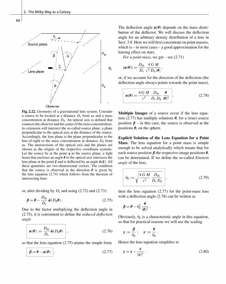
66
2. The Milky Way as a Galaxy
Fig. 2.22. Geometry of a gravitational lens system. Considera source to be located at a distance Ds from us and a massconcentration at distance Dd. An optical axis is defined thatconnects the observer and the center of the mass concentration;its extension will intersect the so-called source plane, a planeperpendicular to the optical axis at the distance of the source.Accordingly, the lens plane is the plane perpendicular to theline-of-sight to the mass concentration at distance Dd fromus. The intersections of the optical axis and the planes arechosen as the origins of the respective coordinate systems.Let the source be at the point η in the source plane; a lightbeam that encloses an angle θ to the optical axis intersects thelens plane at the point ξ and is deflected by an angle α(ξ). Allthese quantities are two-dimensional vectors. The conditionthat the source is observed in the direction θ is given bythe lens equation (2.74) which follows from the theorem ofintersecting lines
or, after dividing by Ds and using (2.72) and (2.73):
β = θ − Dds
Dsα(Ddθ) . (2.75)
Due to the factor multiplying the deflection angle in(2.75), it is convenient to define the reduced deflectionangle
α(θ) := Dds
Dsα(Ddθ) , (2.76)
so that the lens equation (2.75) attains the simple form
β = θ −α(θ) . (2.77)
The deflection angle α(θ) depends on the mass distri-bution of the deflector. We will discuss the deflectionangle for an arbitrary density distribution of a lens inSect. 3.8. Here we will first concentrate on point masses,which is – in most cases – a good approximation for thelensing effect on stars.
For a point mass, we get – see (2.71)
|α(θ)| = Dds
Ds
4 G M
c2 Dd |θ| ,
or, if we account for the direction of the deflection (thedeflection angle always points towards the point mass),
α(θ) = 4 G M
c2
Dds
Ds Dd
θ
|θ|2 . (2.78)
Multiple Images of a source occur if the lens equa-tion (2.77) has multiple solutions θi for a (true) sourceposition β – in this case, the source is observed at thepositions θi on the sphere.
Explicit Solution of the Lens Equation for a PointMass. The lens equation for a point mass is simpleenough to be solved analytically which means that foreach source position β the respective image positions θi
can be determined. If we define the so-called Einsteinangle of the lens,
θE :=√
4 G M
c2
Dds
Ds Dd, (2.79)
then the lens equation (2.77) for the point-mass lenswith a deflection angle (2.78) can be written as
β = θ − θ2E
θ
|θ|2 .
Obviously, θE is a characteristic angle in this equation,so that for practical reasons we will use the scaling
y := β
θE; x := θ
θE.
Hence the lens equation simplifies to
y = x− x|x|2 . (2.80)
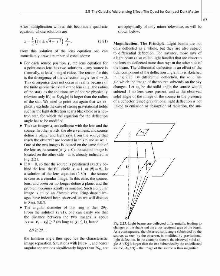
2.5 The Galactic Microlensing Effect: The Quest for Compact Dark Matter
67
After multiplication with x, this becomes a quadraticequation, whose solutions are
x = 1
2
(|y|±
√4+|y|2
) y|y| . (2.81)
From this solution of the lens equation one canimmediately draw a number of conclusions:
• For each source position y, the lens equation fora point-mass lens has two solutions – any source is(formally, at least) imaged twice. The reason for thisis the divergence of the deflection angle for θ → 0.This divergence does not occur in reality because ofthe finite geometric extent of the lens (e.g., the radiusof the star), as the solutions are of course physicallyrelevant only if ξ = DdθE|x| is larger than the radiusof the star. We need to point out again that we ex-plicitly exclude the case of strong gravitational fieldssuch as the light deflection near a black hole or a neu-tron star, for which the equation for the deflectionangle has to be modified.
• The two images xi are collinear with the lens and thesource. In other words, the observer, lens, and sourcedefine a plane, and light rays from the source thatreach the observer are located in this plane as well.One of the two images is located on the same side ofthe lens as the source (x · y > 0), the second image islocated on the other side – as is already indicated inFig. 2.21.
• If y = 0, so that the source is positioned exactly be-hind the lens, the full circle |x| = 1, or |θ| = θE, isa solution of the lens equation (2.80) – the sourceis seen as a circular image. In this case, the source,lens, and observer no longer define a plane, and theproblem becomes axially symmetric. Such a circularimage is called an Einstein ring. Ring-shaped im-ages have indeed been observed, as we will discussin Sect. 3.8.3.
• The angular diameter of this ring is then 2θE.From the solution (2.81), one can easily see thatthe distance between the two images is aboutΔx = |x1 − x2|� 2 (as long as |y|� 1), hence
Δθ � 2θE ;the Einstein angle thus specifies the characteristicimage separation. Situations with |y| � 1, and henceangular separations significantly larger than 2θE, are
astrophysically of only minor relevance, as will beshown below.
Magnification: The Principle. Light beams are notonly deflected as a whole, but they are also subjectto differential deflection. For instance, those rays ofa light beam (also called light bundle) that are closer tothe lens are deflected more than rays at the other side ofthe beam. The differential deflection is an effect of thetidal component of the deflection angle; this is sketchedin Fig. 2.23. By differential deflection, the solid an-gle which the image of the source subtends on the skychanges. Let ωs be the solid angle the source wouldsubtend if no lens were present, and ω the observedsolid angle of the image of the source in the presenceof a deflector. Since gravitational light deflection is notlinked to emission or absorption of radiation, the sur-
Fig. 2.23. Light beams are deflected differentially, leading tochanges of the shape and the cross-sectional area of the beam.As a consequence, the observed solid angle subtended by thesource, as seen by the observer, is modified by gravitationallight deflection. In the example shown, the observed solid an-gle AI/D2
d is larger than the one subtended by the undeflectedsource, AS/D2
s – the image of the source is thus magnified
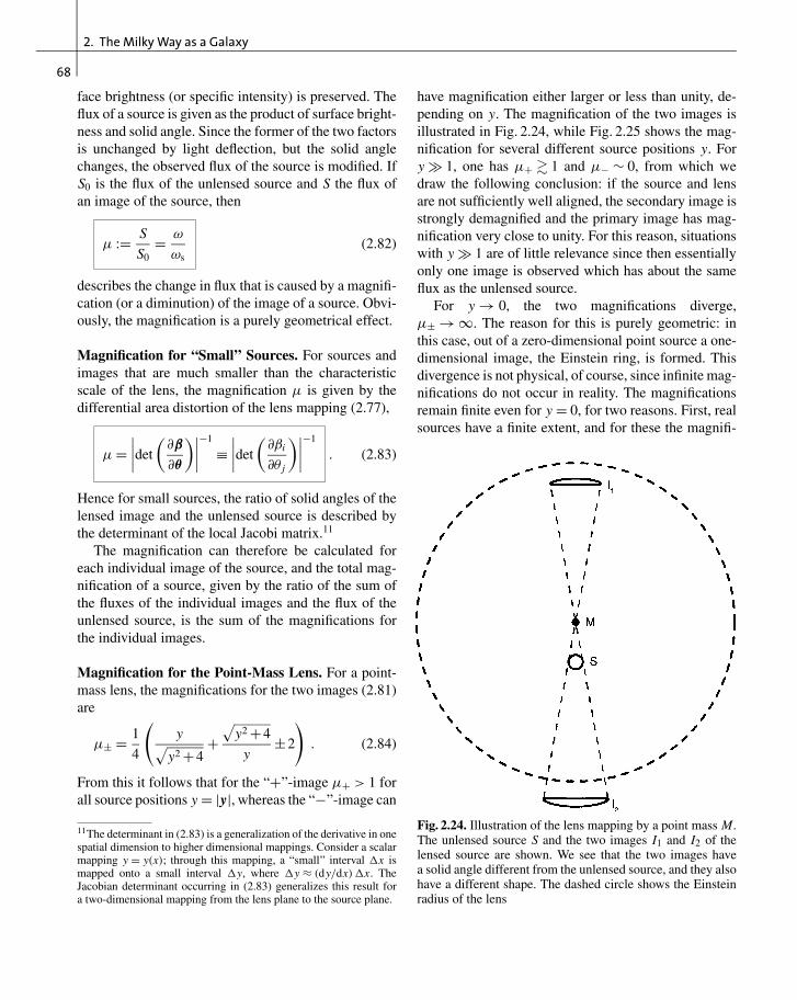
68
2. The Milky Way as a Galaxy
face brightness (or specific intensity) is preserved. Theflux of a source is given as the product of surface bright-ness and solid angle. Since the former of the two factorsis unchanged by light deflection, but the solid anglechanges, the observed flux of the source is modified. IfS0 is the flux of the unlensed source and S the flux ofan image of the source, then
μ := S
S0= ω
ωs(2.82)
describes the change in flux that is caused by a magnifi-cation (or a diminution) of the image of a source. Obvi-ously, the magnification is a purely geometrical effect.
Magnification for “Small” Sources. For sources andimages that are much smaller than the characteristicscale of the lens, the magnification μ is given by thedifferential area distortion of the lens mapping (2.77),
μ =∣∣∣∣det
(∂β
∂θ
)∣∣∣∣−1
≡∣∣∣∣det
(∂βi
∂θ j
)∣∣∣∣−1
. (2.83)
Hence for small sources, the ratio of solid angles of thelensed image and the unlensed source is described bythe determinant of the local Jacobi matrix.11
The magnification can therefore be calculated foreach individual image of the source, and the total mag-nification of a source, given by the ratio of the sum ofthe fluxes of the individual images and the flux of theunlensed source, is the sum of the magnifications forthe individual images.
Magnification for the Point-Mass Lens. For a point-mass lens, the magnifications for the two images (2.81)are
μ± = 1
4
(y√
y2 +4+
√y2 +4
y±2
). (2.84)
From this it follows that for the “+”-image μ+ > 1 forall source positions y = |y|, whereas the “−”-image can
11The determinant in (2.83) is a generalization of the derivative in onespatial dimension to higher dimensional mappings. Consider a scalarmapping y = y(x); through this mapping, a “small” interval Δx ismapped onto a small interval Δy, where Δy ≈ (dy/dx)Δx. TheJacobian determinant occurring in (2.83) generalizes this result fora two-dimensional mapping from the lens plane to the source plane.
have magnification either larger or less than unity, de-pending on y. The magnification of the two images isillustrated in Fig. 2.24, while Fig. 2.25 shows the mag-nification for several different source positions y. Fory � 1, one has μ+ � 1 and μ− ∼ 0, from which wedraw the following conclusion: if the source and lensare not sufficiently well aligned, the secondary image isstrongly demagnified and the primary image has mag-nification very close to unity. For this reason, situationswith y � 1 are of little relevance since then essentiallyonly one image is observed which has about the sameflux as the unlensed source.
For y → 0, the two magnifications diverge,μ± → ∞. The reason for this is purely geometric: inthis case, out of a zero-dimensional point source a one-dimensional image, the Einstein ring, is formed. Thisdivergence is not physical, of course, since infinite mag-nifications do not occur in reality. The magnificationsremain finite even for y = 0, for two reasons. First, realsources have a finite extent, and for these the magnifi-
Fig. 2.24. Illustration of the lens mapping by a point mass M.The unlensed source S and the two images I1 and I2 of thelensed source are shown. We see that the two images havea solid angle different from the unlensed source, and they alsohave a different shape. The dashed circle shows the Einsteinradius of the lens

2.5 The Galactic Microlensing Effect: The Quest for Compact Dark Matter
69
Fig. 2.25. Image of a circular source witha radial brightness profile – indicated bycolors – for different relative positions ofthe lens and source. y decreases from left toright; in the rightmost figure y = 0 and anEinstein ring is formed
cation is finite. Second, even if one had a point source,wave effects of the light (interference) would lead toa finite value of μ. The total magnification of a pointsource by a point-mass lens follows from the sum of themagnifications (2.84),
μ(y) = μ+ +μ− = y2 +2
y√
y2 +4. (2.85)
2.5.2 Galactic Microlensing Effect
After these theoretical considerations we will now re-turn to the starting point of our discussion, employingthe lensing effect as a potential diagnostic for dark mat-ter in our Milky Way, if this dark matter were to consistof compact mass concentrations, e.g., very faint stars.
Image Splitting. Considering a star in our Galaxy asthe lens, (2.79) yields the Einstein angle
θE = 0.902 mas
(M
M�
)1/2
×(
Dd
10 kpc
)−1/2 (1− Dd
Ds
)1/2
. (2.86)
Since the angular separation Δθ of the two images isabout 2θE, the typical image splittings are about a mil-liarcsecond (mas) for lens systems including Galacticstars; such angular separations are as yet not observablewith optical telescopes. This insight made Einstein be-lieve in 1936, after he conducted a detailed quantitativeanalysis of gravitational lensing by point masses, thatthe lens effect will not be observable.12
Magnification. Bohdan Paczynski pointed out in 1986that, although image splitting was unobservable, themagnification by the lens should nevertheless be mea-surable. To do this, we have to realize that the absolutemagnification is observable only if the unlensed flux ofthe source is known – which is not the case, of course(for nearly all sources). However, the magnification,and therefore also the observed flux, changes with timeby the relative motion of source, lens, and ourselves.Therefore, the flux is a function of time, caused by thetime-dependent magnification.
Characteristic Time-Scale of the Variation. Let v bea typical transverse velocity of the lens, then its angularvelocity is
θ = v
Dd= 4.22 mas yr−1
( v
200 km/s
)( Dd
10 kpc
)−1
,
(2.87)
if we consider the source and the observer to be at rest.The characteristic time-scale of the variability is thengiven by
tE := θE
θ= 0.214 yr
(M
M�
)1/2 ( Dd
10 kpc
)1/2
×(
1− Dd
Ds
)1/2 ( v
200 km/s
)−1.
(2.88)
This time-scale is of the order of a month for lenseswith M ∼ M� and typical Galactic velocities. Hence,
12 The expression “microlens” has its origin in the angular scale (2.86)that was discussed in the context of the lens effect on quasars by starsat cosmological distances, for which one obtains image splittings ofabout one microarcsecond.
70
2. The Milky Way as a Galaxy
the effect is measurable in principle. In the general casethat source, lens, and observer are all moving, v hasto be considered as an effective velocity. Alternatively,the motion of the source in the source plane can beconsidered.
Light Curves. In most cases, the relative motion can beconsidered linear, so that the position of the source inthe source plane can be written as
β = β0 + β(t − t0) .
Using the scaled position y = β/θE, for y = |y| weobtain
y(t) =√
p2 +(
t − tmax
tE
)2
, (2.89)
where p = ymin specifies the minimum distance fromthe optical axis, and tmax is the time at which y = pattains this minimum value, thus when the magnificationμ = μ(p) = μmax is maximized. From this, and using(2.85), one obtains the light curve
S(t) = S0 μ(y(t)) = S0y2(t)+2
y(t)√
y2(t)+4. (2.90)
Examples for such light curves are shown in Fig. 2.26.They depend on only four parameters: the flux of theunlensed source S0, the time of maximum magnifica-tion tmax, the smallest distance of the source from theoptical axis p, and the characteristic time-scale tE. Allthese values are directly observable in a light curve. Oneobtains tmax from the time of the maximum of the lightcurve, S0 is the flux that is measured for very largeand small times, S0 = S(t → ±∞), or S0 ≈ S(t) for|t − tmax| � tE. Furthermore, p follows from the max-imum magnification μmax = Smax/S0 by inversion of(2.85), and tE from the width of the light curve.
Only tE contains information of astrophysical rele-vance, because the time of the maximum, the unlensedflux of the source, and the minimum separation pprovide no information about the lens. Since tE ∝√
M Dd/v, this time-scale contains the combined in-formation on the lens mass, the distances to the lens andthe source, and the transverse velocity: Only the com-bination tE ∝ √
M Dd/v can be derived from the lightcurve, but not mass, distance, or velocity individually.
Paczynski’s idea can be expressed as follows: if thehalo of our Milky Way consists (partially) of compactobjects, a distant compact source should, from time totime, be lensed by one of these MACHOs and thus showcharacteristic changes in flux, corresponding to a lightcurve similar to those in Fig. 2.26. The number densityof MACHOs is proportional to the probability or abun-dance of lens events, and the characteristic mass of theMACHOs is proportional to the square of the typicalvariation time-scale tE. All one has to do is measurethe light curves of a sufficiently large number of back-ground sources and extract all lens events from thoselight curves to obtain information on the population ofpotential MACHOs in the halo. A given halo modelpredicts the spatial density distribution and the distribu-tion of velocities of the MACHOs and can therefore becompared to the observations in a statistical way. How-ever, one faces the problem that the abundance of suchlensing events is very small.
Probability of a Lens Event. In practice, a system ofa foreground object and a background source is con-sidered a lens system if p < 1 and hence μmax > 3/
√5
≈ 1.34, i.e., if the relative trajectory of the source passeswithin the Einstein circle of the lens.
If the dark halo of the Milky Way consisted solely ofMACHOs, the probability that a very distant source islensed (in the sense of |β| ≤ θE) would be ∼ 10−7, wherethe exact value depends on the direction to the source.At any one time, one of ∼ 107 distant sources would belocated within the Einstein radius of a MACHO in ourhalo. The immediate consequence of this is that the lightcurves of millions of sources have to be monitored todetect this effect. Furthermore, these sources have to belocated within a relatively small region on the sphere tokeep the total solid angle that has to be photometricallymonitored relatively small. This condition is needed tolimit the required observing time, so that many suchsources should be present within the field-of-view ofthe camera used. The stars of the Magellanic Cloudsare well suited for such an experiment: they are closetogether on the sphere, but can still be resolved intoindividual stars.
Problems, and their Solution. From this observationalstrategy, a large number of problems arise immediately;they were discussed in Paczynski’s original paper. First,

2.5 The Galactic Microlensing Effect: The Quest for Compact Dark Matter
71
Fig. 2.26. Illustration of a Galactic microlensing event: In theupper left panel a source (depicted by the open circles) movesbehind a point-mass lens; for each source position two imagesof the source are formed, which are indicated by the blackellipses. The identification of the corresponding image pairwith the source position follows from the fact that, in pro-jection, the source, the lens, and the two images are locatedon a straight line, which is indicated for one source position.
The dashed circle represents the Einstein ring. In the lower leftpanel, different trajectories of the source are shown, each char-acterized by the smallest projected separation p to the lens.The light curves resulting from these relative motions, whichcan be calculated using equation (2.90), are then shown in theright-hand panel for different values of p. The smaller p is,the larger the maximum magnification will be, here measuredin magnitudes
the photometry of so many sources over many epochsproduces a huge amount of data that need to be handled;they have to be stored and reduced. Second, one has theproblem of “crowding”: the stars in the MagellanicClouds are densely packed on the sky, which rendersthe photometry of individual stars difficult. Third, starsalso show intrinsic variability – about 1% of all starsare variable. This intrinsic variability has to be distin-guished from that due to the lens effect. Due to the
small abundance of the latter, selecting the lens eventsis comparable to searching for a needle in a haystack.Finally, it should be mentioned that one has to ensurethat the experiment is indeed sensitive enough to detectlens events. A “calibration experiment” would thereforebe desirable.
Faced with these problems, it seemed daring to seri-ously think about the realization of such an observingprogram. However, a fortunate event helped, in the mag-
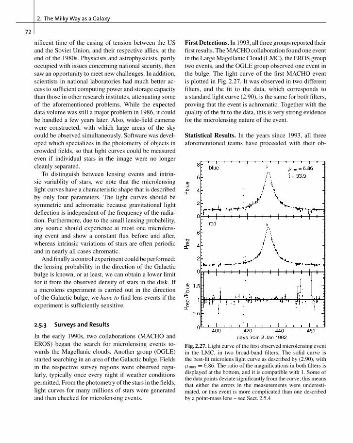
72
2. The Milky Way as a Galaxy
nificent time of the easing of tension between the USand the Soviet Union, and their respective allies, at theend of the 1980s. Physicists and astrophysicists, partlyoccupied with issues concerning national security, thensaw an opportunity to meet new challenges. In addition,scientists in national laboratories had much better ac-cess to sufficient computing power and storage capacitythan those in other research institutes, attenuating someof the aforementioned problems. While the expecteddata volume was still a major problem in 1986, it couldbe handled a few years later. Also, wide-field cameraswere constructed, with which large areas of the skycould be observed simultaneously. Software was devel-oped which specializes in the photometry of objects incrowded fields, so that light curves could be measuredeven if individual stars in the image were no longercleanly separated.
To distinguish between lensing events and intrin-sic variablity of stars, we note that the microlensinglight curves have a characteristic shape that is describedby only four parameters. The light curves should besymmetric and achromatic because gravitational lightdeflection is independent of the frequency of the radia-tion. Furthermore, due to the small lensing probability,any source should experience at most one microlens-ing event and show a constant flux before and after,whereas intrinsic variations of stars are often periodicand in nearly all cases chromatic.
And finally a control experiment could be performed:the lensing probability in the direction of the Galacticbulge is known, or at least, we can obtain a lower limitfor it from the observed density of stars in the disk. Ifa microlens experiment is carried out in the directionof the Galactic bulge, we have to find lens events if theexperiment is sufficiently sensitive.
2.5.3 Surveys and Results
In the early 1990s, two collaborations (MACHO andEROS) began the search for microlensing events to-wards the Magellanic clouds. Another group (OGLE)started searching in an area of the Galactic bulge. Fieldsin the respective survey regions were observed regu-larly, typically once every night if weather conditionspermitted. From the photometry of the stars in the fields,light curves for many millions of stars were generatedand then checked for microlensing events.
First Detections. In 1993, all three groups reported theirfirst results. The MACHO collaboration found one eventin the Large Magellanic Cloud (LMC), the EROS grouptwo events, and the OGLE group observed one event inthe bulge. The light curve of the first MACHO eventis plotted in Fig. 2.27. It was observed in two differentfilters, and the fit to the data, which corresponds toa standard light curve (2.90), is the same for both filters,proving that the event is achromatic. Together with thequality of the fit to the data, this is very strong evidencefor the microlensing nature of the event.
Statistical Results. In the years since 1993, all threeaforementioned teams have proceeded with their ob-
Fig. 2.27. Light curve of the first observed microlensing eventin the LMC, in two broad-band filters. The solid curve isthe best-fit microlens light curve as described by (2.90), withμmax = 6.86. The ratio of the magnifications in both filters isdisplayed at the bottom, and it is compatible with 1. Some ofthe data points deviate significantly from the curve; this meansthat either the errors in the measurements were underesti-mated, or this event is more complicated than one describedby a point-mass lens – see Sect. 2.5.4

2.5 The Galactic Microlensing Effect: The Quest for Compact Dark Matter
73
servations and analysis (Fig. 2.28), and more groupshave begun the search for microlensing events, choos-ing various lines-of-sight. The most important resultsfrom these experiments can be summarized as follows:
About 20 events have been found in the directionof the Magellanic Clouds, and of the order a thousandin the direction of the bulge. The statistical analysis ofthe data revealed the lensing probability towards thebulge to be higher than originally expected. This canbe explained by the fact that our Galaxy features a bar(see Chap. 3). This bar was also observed in IR mapssuch as those made by the COBE satellite. The eventsin the direction of the bulge are dominated by lensesthat are part of the bulge themselves, and their columndensity is increased by the bar-like shape of the bulge.On the other hand, the lens probability in the direction ofthe Magellanic Clouds is smaller than expected for thecase where the dark halo consists solely of MACHOs.
Fig. 2.28. In this 8◦ ×8◦ image of the LMC, 30 fields aremarked in red which the MACHO group has searched for mi-crolensing events during the ∼ 5.5 years of their experiment;images were taken in two filters to test for achromaticity. Thepositions of 17 microlens events are marked by yellow circles;these have been subject to statistical analysis
Based on the analysis of the MACHO collaboration,the observed statistics of lensing events towards theMagellanic Clouds is best explained if about 20% of thehalo mass consists of MACHOs, with a characteristicmass of about M ∼ 0.5M� (see Fig. 2.29).
Interpretation and Discussion. This latter result is noteasy to interpret and came as a real surprise. If a resultcompatible with ∼ 100% had been found, it would havebeen obvious to conclude that the dark matter in ourMilky Way consists of compact objects. Otherwise, ifvery few lensing events had been found, it would havebeen clear that MACHOs do not contribute significantlyto the dark matter. But a value of 20% does not allowany unambiguous interpretation. Taken at face value,the result from the MACHO group would imply that thetotal mass of MACHOs in the Milky Way halo is aboutthe same as that in the stellar disk.
Furthermore, the estimated mass scale is hard to un-derstand: what could be the nature of MACHOs withM = 0.5M�? Normal stars can be excluded, becausethey would be far too luminous not to be observed.White dwarfs are also unsuitable candidates, because to
Fig. 2.29. Probability contours for a specific halo model asa function of the characteristic MACHO mass M (here denotedby m) and the mass fraction f of MACHOs in the halo. Thehalo of the LMC was either taken into account as an additionalsource for microlenses (lmc halo) or not (no lmc halo), and twodifferent selection criteria (A,B) for the statistically completemicrolensing sample have been used. In all cases, M ∼ 0.5M�and f ∼ 0.2 are the best-fit values

74
2. The Milky Way as a Galaxy
produce such a large number of white dwarfs as a fi-nal stage of stellar evolution, the total star formationin our Milky Way, integrated over its lifetime, needsto be significantly larger than normally assumed. Inthis case, many more massive stars would also haveformed, which would then have released the metals theyproduced into the ISM, both by stellar winds and in su-pernova explosions. In such a scenario, the metal contentof the ISM would therefore be distinctly higher than isactually observed. The only possibility of escaping thisargument is with the hypothesis that the mass functionof newly formed stars (the initial mass function, IMF)was different in the early phase of the Milky Way com-pared to that observed today. The IMF that needs to beassumed in this case is such that for each star of interme-diate mass which evolves into a white dwarf, far fewerhigh-mass stars, responsible for the metal enrichmentof the ISM, must have formed in the past comparedto today. However, we lack a plausible physical modelfor such a scenario, and it is in conflict with the star-formation history that we observe in the high-redshiftUniverse (see Chap. 9).
Neutron stars can be excluded as well, becausethey are too massive (typically > 1M�); in addition,they are formed in supernova explosions, implying thatthe aforementioned metallicity problem would be evengreater for neutron stars. Would stellar-mass black holesbe an alternative? The answer to this question dependson how they are formed. They could not originate in SNexplosions, again because of the metallicity problem.If they had formed in a very early phase of the Uni-verse (they are then called primordial black holes), thiswould be an imaginable, though perhaps quite exotic,alternative.
However, we have strong indications that theinterpretation of the MACHO results is not as straight-forward as described above. Some doubts have beenraised as to whether all events reported as being due tomicrolensing are in fact caused by this effect. In fact,one of the microlensing source stars identified by theMACHO group showed another bump seven years afterthe first event. Given the extremely small likelihood oftwo microlensing events happening to a single sourcethis is almost certainly a star with unusual variability.
As argued previously, by means of tE we only mea-sure a combination of lens mass, transverse velocity,and distance. The result given in Fig. 2.29 is therefore
based on the statistical analysis of the lensing eventsin the framework of a halo model that describes theshape and the radial density profile of the halo. How-ever, microlensing events have been observed for whichmore than just tE can be determined – e.g., events inwhich the lens is a binary star, or those for which tEis larger than a few months. In this case, the orbit ofthe Earth around the Sun, which is not a linear motion,has a noticeable effect, causing deviations from thestandard curve. Such parallax events have indeed beenobserved.13 Three events are known in the direction ofthe Magellanic Clouds in which more than just tE couldbe measured. In all three cases the lenses are most likelylocated in the Magellanic Clouds themselves (an effectcalled self-lensing) and not in the halo of the MilkyWay. If for those three cases, where the degeneracy be-tween lens mass, distance, and transverse velocity canbe broken, the respective lenses are not MACHOs in theGalactic halo, we might then suspect that in most of theother microlensing events the lens is not a MACHO ei-ther. Therefore, it is currently unclear how to interpretthe results of the microlensing surveys. In particular, itis unclear to what extent self-lensing contributes to theresults. Furthermore, the quantitative results depend onthe halo model.
The EROS collaboration used an observation strategywhich was sightly different from that of the MACHOgroup, by observing a number of fields in very short timeintervals. Since the duration of a lensing event dependson the mass of the lens as Δt ∝ M1/2 – see (2.88) – theywere also able to probe very small MACHO masses.The absence of lensing events of very short durationthen allowed them to derive limits for the mass fractionof such low-mass MACHOs, as is shown in Fig. 2.30.
Despite this unsettled situation concerning the inter-pretation of the MACHO results, we have to emphasizethat the microlensing surveys have been enormouslysuccessful experiments because they accomplishedexactly what was expected at the beginning of the ob-servations. They measured the lensing probability inthe direction of the Magellanic Clouds and the Galacticbulge. The fact that the distribution of the lenses differsfrom that expected by no means diminishes the successof these surveys.
13 These parallax events in addition prove that the Earth is in factorbiting around the Sun – even though this is not really a new insight.

2.5 The Galactic Microlensing Effect: The Quest for Compact Dark Matter
75
Fig. 2.30. From observations by the EROS collaboration,a large mass range for MACHO candidates can be excluded.The maximum allowed fraction of the halo mass containedin MACHOs is plotted as a function of the MACHO massM, as an upper limit with 95% confidence. A standard modelfor the mass distribution in the Galactic halo was assumedwhich describes the rotation curve of the Milky Way quitewell. The various curves show different phases of the EROSexperiment. They are plotted separately for observations in
the directions of the LMC and the SMC. The experimentEROS 1 searched for microlensing events on short time-scales but did not find any; this yields the upper limits atsmall masses. Upper limits at larger masses were obtainedby the EROS 2 experiment. The thick solid curve representsthe upper limit derived from combining the individual ex-periments. If not a single MACHO event had been foundthe upper limit would have been described by the dottedline
2.5.4 Variations and Extensions
Besides the search for MACHOs, microlensing surveyshave yielded other important results and will continue todo so in the future. For instance, the distribution of starsin the Galaxy can be measured by analyzing the lens-ing probability as a function of direction. Thousandsof variable stars have been newly discovered and accu-rately monitored; the extensive and publicly accessibledatabases of the surveys form an invaluable resourcefor stellar astrophysics. Furthermore, globular clustersin the LMC have been identified from these photometricobservations.
For some lensing events, the radius and the surfacestructure of distant stars can be measured with very highprecision. This is possible because the magnification μ
depends on the position of the source. Situations can oc-cur, for example where a binary star acts as a lens (seeFig. 2.31), in which the dependence of the magnifica-tion on the position in the source plane is very sensitive.Since the source – the star – is in motion relative to theline-of-sight between Earth and the lens, its different
regions are subject to different magnification, depend-ing on the time-dependent source position. A detailedanalysis of the light curve of such events then enablesus to reconstruct the light distribution on the surface ofthe star. The light curve of one such event is shown inFig. 2.32.
For these lensing events the source can no longerbe assumed to be a point source. Rather, the details ofthe light curve are determined by its light distribution.Therefore, another length-scale appears in the system,the radius of the star. This length-scale shows up in thecorresponding microlensing light curve, as can be seenin Fig. 2.32, by the time-scale which characterizes thewidth of the peaks in the light curve – it is directly re-lated to the ratio of the stellar radius and the transversevelocity of the lens. With this new scale, the degener-acy between M, v, and Dd is partially broken, so thatthese special events provide more information than the“classical” ones.
In fact, the light curve in Fig. 2.27 is probably notcaused by a single lens star, but instead by additionalslight disturbances from a companion star. This would

76
2. The Milky Way as a Galaxy
Fig. 2.31. If a binary star acts as a lens, significantly more com-plicated light curves can be generated. In the left-hand paneltracks are plotted for five different relative motions of a back-ground source; the dashed curve is the so-called critical curve,formally defined by det(∂β/∂θ) = 0, and the solid line is thecorresponding image of the critical curve in the source plane,called a caustic. Light curves corresponding to these five
tracks are plotted in the right-hand panel. If the source crossesthe caustic, the magnification μ becomes very large – formallyinfinite if the source was point-like. Since it has a finite extent,μ has to be finite as well; from the maximum μ during caus-tic crossing, the radius of the source can be determined, andsometimes even the variation of the surface brightness acrossthe stellar disk, an effect known as limb darkening
explain the deviation of the observed light curve froma simple model light curve. However, the sampling intime of this particular light curve is not sufficient todetermine the parameters of the binary system.
By now, detailed light curves with very good timecoverage have been measured, which was made possi-ble with an alarm system. The data from those groupssearching for microlensing events are analyzed imme-diately after observations, and potential candidates forinteresting events are published on the Internet. Othergroups (such as the PLANET collaboration, for ex-ample) then follow-up these systems with very goodtime coverage by using several telescopes spread overa large range in geographical longitude. This makesaround-the-clock observations of the event possible.Using this method light curves of extremely high qual-ity have been measured. These groups hope to detectextra-solar planets by characteristic deviations in theselight curves. Indeed, these microlens observations maybe the most realistic (and cheapest) option for findinglow-mass planets. Other methods for finding extra-solarplanets, such as the search for small periodic changesof the radial velocity of stars which is caused by thegravitational pull of their orbiting planet, are mostlysensitive to high-mass planets. Whereas such surveys
Fig. 2.32. Light curve of an event in which the lens was a bi-nary star. The MACHO group discovered this “binary event”.Members of the PLANET collaboration obtained this data us-ing four different telescopes (in Chile, Tasmania, and SouthAfrica). The second caustic crossing is highly resolved (dis-played in the small diagram) and allows us to draw conclusionsabout the size and the brightness distribution of the source star.The two curves show the fits of a binary lens to the data
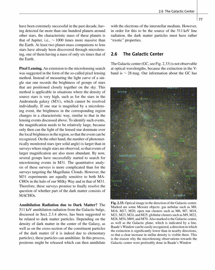
2.6 The Galactic Center
77
have been extremely successful in the past decade, hav-ing detected far more than one hundred planets aroundother stars, the characteristic mass of these planets isthat of Jupiter, i.e., ∼ 1000 times more massive thanthe Earth. At least two planet-mass companions to lensstars have already been discovered through microlens-ing, one of them having a mass of only six times that ofthe Earth.
Pixel Lensing. An extension to the microlensing searchwas suggested in the form of the so-called pixel lensingmethod. Instead of measuring the light curve of a sin-gle star one records the brightness of groups of starsthat are positioned closely together on the sky. Thismethod is applicable in situations where the density ofsource stars is very high, such as for the stars in theAndromeda galaxy (M31), which cannot be resolvedindividually. If one star is magnified by a microlens-ing event, the brightness in the corresponding regionchanges in a characteristic way, similar to that in thelensing events discussed above. To identify such events,the magnification needs to be relatively large, becauseonly then can the light of the lensed star dominate overthe local brightness in the region, so that the event can berecognized. On the other hand, the number of photomet-rically monitored stars (per solid angle) is larger than insurveys where single stars are observed, so that events oflarger magnification are also more abundant. By now,several groups have successfully started to search formicrolensing events in M31. The quantitative analy-sis of these surveys is more complicated than for thesurveys targeting the Magellanic Clouds. However, theM31 experiments are equally sensitive to both MA-CHOs in the halo of our Milky Way and in that of M31.Therefore, these surveys promise to finally resolve thequestion of whether part of the dark matter consists ofMACHOs.
Annihilation Radiation due to Dark Matter? The511 keV annihilation radiation from the Galactic bulge,discussed in Sect. 2.3.4 above, has been suggested tobe related to dark matter particles. Depending on thedensity of dark matter in the center of the Galaxy, aswell as on the cross-section of the constituent particlesof the dark matter (if it is indeed due to elementaryparticles), these particles can annihilate. In this process,positrons might be released which can then annihilate
with the electrons of the interstellar medium. However,in order for this to be the source of the 511 keV lineradiation, the dark matter particles must have rather“exotic” properties.
2.6 The Galactic Center
The Galactic center (GC, see Fig. 2.33) is not observableat optical wavelengths, because the extinction in the V-band is ∼ 28 mag. Our information about the GC has
Fig. 2.33. Optical image in the direction of the Galactic center.Marked are some Messier objects: gas nebulae such as M8,M16, M17, M20; open star clusters such as M6, M7, M18,M21, M23, M24, and M25; globular clusters such as M9, M22,M28, M54, M69, and M70. Also marked is the Galactic center,as well as the Galactic plane, which is indicated by a line.Baade’s Window can be easily recognized, a direction in whichthe extinction is significantly lower than in nearby directions,so that a clear increase in stellar density is visible there. Thisis the reason why the microlensing observations towards theGalactic center were preferably done in Baade’s Window

78
2. The Milky Way as a Galaxy
been obtained from radio-, IR-, and X-ray radiation.Since the GC is nearby, and thus serves as a prototypeof the central regions of galaxies, its observation is ofgreat interest for our understanding of the processestaking place in the centers of galaxies.
2.6.1 Where is the Galactic Center?
The question of where the center of our Milky Way islocated is by no means trivial, because the term “center”is in fact not well-defined. Is it the center of mass of theGalaxy, or the point around which the stars and the gasare orbiting? And how could we pinpoint this “center”accurately? Fortunately, the center can nevertheless belocalized because, as we will see below, a distinct sourceexists that is readily identified as the Galactic center.
Radio observations in the direction of the GC showa relatively complex structure, as is displayed in Fig.2.34.
A central disk of HI gas exists at radii from several100 pc up to about 1 kpc. Its rotational velocity yieldsa mass estimate M(R) for R � 100 pc. Furthermore,radio filaments are observed which extend perpendicu-larly to the Galactic plane, and also a large number ofsupernova remnants are seen. Within about 2 kpc fromthe center, roughly 3×10⁷ M� of atomic hydrogen isfound. Optical images show regions close to the GCtowards which the extinction is significantly lower. Thebest known of these is Baade’s window – most of themicrolensing surveys towards the bulge are conductedin this region. In addition, a fairly large number of glob-ular clusters and gas nebulae are observed towards thecentral region. X-ray images (Fig. 2.35) show numerousX-ray binaries, as well as diffuse emission by hot gas.
The innermost 8 pc contain the radio source Sgr A(Sagittarius A), which itself consists of differentcomponents:
• A circumnuclear molecular ring, shaped like a torus,which extends between radii of 2 pc� R � 8 pc andis inclined by about 20◦ relative to the Galacticdisk. The rotational velocity of this ring is about∼ 110 km/s, nearly independent of R. This ring hasa sharp inner boundary; this cannot be the result of anequilibrium flow, because internal turbulent motionswould quickly (on a time-scale of ∼ 105 yr) erasethis boundary. Probably, it is evidence of an ener-
getic event that occurred in the Galactic center withinthe past ∼ 105 years. This interpretation is also sup-ported by other observations, e.g., by a clumpinessin density and temperature.
• Sgr A East, a non-thermal (synchrotron) source ofshell-like structure. Presumably this is a supernovaremnant (SNR), with an age between 100 and 5000years.
• Sgr A West is located about 1.′5 away from SgrA East. It is a thermal source, an unusual HII regionwith a spiral-like structure.
• Sgr A∗ is a strong compact radio source close to thecenter of Sgr A West. Recent observations with mm-VLBI show that its extent is smaller than 3 AU. Theradio luminosity is L rad ∼ 2×1034 erg/s. Except forthe emission in the mm and cm domain, Sgr A∗ isa weak source. Since other galaxies often have a com-pact radio source in their center, Sgr A∗ is an excellentcandidate for being the center of our Milky Way.
Through observations of stars which contain a radiomaser14 source, the astrometry of the GC in the radiodomain was matched to that in the IR, i.e., the positionof Sgr A∗ is also known in the IR.15 The uncertainty inthe relative positions between radio and IR observationsis only ∼ 30 mas – at a presumed distance of the GC of8 kpc, one arcsecond corresponds to 0.0388 pc, or about8000 AU.
2.6.2 The Central Star Cluster
Density Distribution. Observations in the K-band(λ ∼ 2 μm) show a compact star cluster that is cen-tered on Sgr A∗. Its density behaves like ∝ r−1.8 in thedistance range 0.1 pc� r � 1 pc. The number density
14 Masers are regions of stimulated non-thermal emission which showa very high surface brightness. The maser phenomenon is similar tothat of lasers, except that the former radiate in the microwave regimeof the spectrum. Masers are sometimes found in the atmospheres ofactive stars.15 One problem in the combined analysis of data taken in differentwavelength bands is that astrometry in each individual wavelengthband can be performed with a very high precision – e.g., individu-ally in the radio and the IR band – however, the relative astrometrybetween these bands is less well known. To stack maps of differentwavelength precisely “on top of each other”, knowledge of exact rel-ative astrometry is essential. This can be gained if a population ofcompact sources exists that is observable in both wavelength domainsand for which accurate positions can be measured.

2.6 The Galactic Center
79
Fig. 2.34. Left: A VLA wide-field image of the region aroundthe Galactic center, with a large number of sources identified.Upper right: a 20 cm continuum VLA image of Sgr A East,
where the red dot marks Sgr A∗. Center right: Sgr A West,as seen in a 6-cm continuum VLA image. Lower right: thecircumnuclear ring in HCN line emission
of stars in its inner region is so large that close stellarencounters are common. It can be estimated that a starhas a close encounter about every ∼ 106 years. Thus, itis expected that the distribution of the stars is “thermal-ized”, which means that the local velocity distributionof the stars is the same everywhere, i.e., it is close toa Maxwellian distribution with a constant velocity dis-persion. For such an isothermal distribution we expect
a density profile n ∝ r−2, which is in good agreementwith the observation.
However, another observational result yields a strik-ing and interesting discrepancy with respect to the ideaof an isothermal distribution. Instead of the expectedconstant dispersion σ of the radial velocities of the stars,a strong radial dependence is observed: σ increases to-wards smaller r. For example, one finds σ ∼ 55 km/s at

80
2. The Milky Way as a Galaxy
Fig. 2.35. Mosaic of X-ray images of the Galactic center, takenby the Chandra satellite. The image covers an area of about130 pc×300 pc (48′ ×120′). The actual GC, in which a su-permassive black hole is suspected to reside, is located inthe white region near the center of the image. Furthermore,on this image hundreds of white dwarfs, neutron stars, and
black holes are visible that radiate in the X-ray regime dueto accretion phenomena (accreting X-ray binaries). Colorscode the photon energy, from low energy (red) to high energy(blue). The diffuse emission, predominantly red in this im-age, originates in diffuse hot gas with a temperature of aboutT ∼ 107 K
r = 5 pc, but σ ∼ 180 km/s at r = 0.15 pc. This discrep-ancy indicates that the gravitational potential in whichthe stars are moving is generated not only by themselves.According to the virial theorem, the strong increase ofσ for small r implies the presence of a central massconcentration in the star cluster.
Proper Motions. Since the middle of the 1990s, propermotions of stars in this star cluster have also been mea-sured, using the methods of speckle interferometry andadaptive optics. These produce images at diffraction-limited angular resolution, about ∼ 0′′. 15 in the K-bandat the ESO/NTT (3.5 m) and about ∼ 0′′. 05 at the Keck(10 m). Proper motions are currently known for about1000 stars within ∼ 10′′ of Sgr A∗. This breakthroughwas achieved independently by two groups, whose re-sults are in excellent agreement. For more than 20 starswithin ∼ 5′′ of Sgr A∗ both proper motions and radial ve-locities, and therefore their three-dimensional velocitiesare known. The radial and tangential velocity disper-sions resulting from these measurements are in goodmutual agreement. Thus, it can be concluded that a ba-sically isotropic distribution of the stellar orbits exists,simplifying the study of the dynamics of this stellarcluster.
The Origin of Very Massive Stars near the GalacticCenter. One of the unsolved problems is the presenceof these massive stars close to the Galactic center. One
finds that most of the innermost stars are main-sequenceB-stars. Their small lifetime of ∼ 108 yr probably im-plies that these stars were born close to the Galacticcenter. This, however, is very difficult to understand.Both the strong tidal gravitational field of the centralblack hole (see below) and the presumably strong mag-netic field in this region will prevent the “standard”star-formation picture of a collapsing molecular cloud:the former effect tends to disrupt such a cloud whilethe latter stabilizes it against gravitational contraction.Several solutions to this problem have been suggested,such as a scenario in which the stars are born at largerdistances from the Galactic center and then broughtthere by dynamical processes, involving strong gravita-tional scattering events. However, none of these modelsappears satisfactory at present.
2.6.3 A Black Hole in the Center of the Milky Way
Some stars within 0′′. 6 of Sgr A∗ have a proper motionof more than 1000 km/s, as shown in Fig. 2.36. Forinstance, the star S1 has a separation of only 0′′. 1 fromSgr A∗ and shows proper motion of 1470 km/s at theepoch displayed in Fig. 2.36. Combining the velocitydispersions in radial and tangential directions revealsit to be increasing according to the Kepler law for thepresence of a point mass, σ ∝ r−1/2 down to r ∼ 0.01 pc.
By now, the acceleration of some stars in the starcluster has also been measured, i.e., the change of proper

2.6 The Galactic Center
81
Fig. 2.36. Proper motions of stars in thecentral region of the GC. The differentlycolored arrows denote different types ofstars. The small image shows the propermotions in the Sgr A∗ star cluster within halfan arcsecond from Sgr A∗; the fastest star(S1) has a proper motion of ∼ 1500 km/s(from Genzel, 2000, astro-ph/0008119
motion with time. From these measurements Sgr A∗ in-deed emerges as the focus of the orbits and thus as thecenter of mass. Figure 2.37 shows the orbits of somestars around Sgr A∗. The star S2 could be observedduring a major fraction of its orbit, where a maximumvelocity of more than 5000 km/s was found. The eccen-tricity of the orbit of S2 is 0.87, and its orbital periodis ∼ 15.7 yr. The minimum separation of this star fromSgr A∗ is only 6×10⁻⁴ pc, or about 100 AU.
From the observed kinematics, the enclosed massM(r) can be calculated, see Fig. 2.38. The correspond-ing analysis yields that M(r) is basically constant overthe range 0.01 pc � r � 0.5 pc. This exciting resultclearly indicates the presence of a point mass, for whicha mass of
M = (3.6±0.4)×106 M� (2.91)
is determined. For larger radii, the mass of the star clus-ter dominates; it nearly follows an isothermal densitydistribution with a core radius of ∼ 0.34 pc and a centraldensity of 3.6×10⁶ M�/pc3. This result is also compat-ible with the kinematics of the gas in the center of theGalaxy. However, stars are much better kinematic indi-cators because gas can be affected by magnetic fields,viscosity, and various other processes besides gravity.
The kinematics of stars in the central star clusterof the Galaxy shows that our Milky Way containsa mass concentration in which ∼ 3×10⁶ M� areconcentrated within a region smaller than 0.01 pc.This is most probably a black hole in the centerof our Galaxy at the position of the compact radiosource Sgr A∗.
Why a Black Hole? We have interpreted the centralmass concentration as a black hole; this requires somefurther explanation:
• The energy for the central activity in quasars, radiogalaxies, and other AGNs is produced by accretion ofgas onto a supermassive black hole (SMBH); we willdiscuss this in more detail in Sect. 5.3. Thus we knowthat at least a subclass of galaxies contains a centralSMBH. Furthermore, we will see in Sect. 3.5 thatmany “normal” galaxies, especially ellipticals, har-bor a black hole in their center. The presence ofa black hole in the center of our own Galaxy wouldtherefore not be something unusual.
• To bring the radial mass profile M(r) into accordancewith an extended mass distribution, its density dis-tribution must be very strongly concentrated, witha density profile steeper than ∝ r−4; otherwise the

82
2. The Milky Way as a Galaxy
Fig. 2.37. At left, the or-bit of the star S2 aroundSgr A∗ is shown as de-termined by two differentobserving campaigns. Theposition of Sgr A∗ isindicated by the black cir-cled cross. The individualpoints along the orbit areidentified by the epochof the observation. Theright-hand image showsthe orbits of some otherstars for which accelera-tions have already beenmeasured
mass profile M(r) would not be as flat as observed inFig. 2.38. Hence, this hypothetical mass distributionmust be vastly different from the expected isother-mal distribution which has a mass profile ∝ r−2, asdiscussed in Sect. 2.6.2. However, observations ofthe stellar distribution provide no indication of aninwardly increasing density of the star cluster withsuch a steep profile.
• Even if such an ultra-dense star cluster (with a centraldensity of � 4×10¹² M�/pc3) were present it couldnot be stable, but instead would dissolve within ∼ 107
years through frequent stellar collisions.• Sgr A∗ itself has a proper motion of less than
20 km/s. It is therefore the dynamic center ofthe Milky Way. Due to the large velocities of itssurrounding stars, one would derive a mass ofM � 103 M� for the radio source, assuming equipar-tition of energy (see also Sect. 2.6.5). Together withthe tight upper limits for its extent, a lower limit forthe density of 1018 M�/pc3 can then be obtained.
Following the stellar orbits in forthcoming years willfurther complete our picture of the mass distribution inthe GC.
We have to emphasize at this point that the gravi-tational effect of the black hole on the motion of starsand gas is constrained to the innermost region of the
Milky Way. As one can see from Fig. 2.38, the gravita-tional field of the SMBH dominates the rotation curveof the Galaxy only for R� 2 pc – this is the very reasonwhy the detection of the SMBH is so difficult. At largerradii, the presence of the SMBH is of no relevance forthe rotation curve of the Milky Way.
2.6.4 Flares from the Galactic Center
In 2000, the X-ray satellite Chandra discovered a power-ful X-ray flare from Sgr A∗. This event lasted for aboutthree hours, and the X-ray flux increased by a factorof 50 during this period. XMM-Newton confirmed theexistence of X-ray flares, recording one where the lu-minosity increased by a factor of ∼ 200. Combining theflare duration of a few hours with the short time-scaleof variability of a few minutes indicates that the emis-sion must originate from a very small source, not largerthan ∼ 1013 cm in size.
Monitoring Sgr A∗ in the NIR, flare emission wasalso found in this spectral regime. These NIR flaresare more frequent than in X-rays, occurring severaltimes per day. Furthermore, the NIR emission seemsto show some sort of periodicity of ∼ 17 min, which ismost likely to be identified with an orbital motion ofthe emitting material around the SMBH. Indeed, a re-analysis of the X-ray light curve shows some hint of
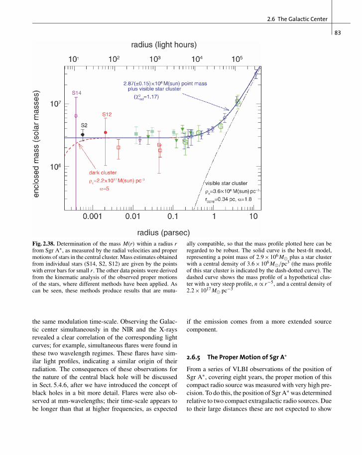
2.6 The Galactic Center
83
Fig. 2.38. Determination of the mass M(r) within a radius rfrom Sgr A∗, as measured by the radial velocities and propermotions of stars in the central cluster. Mass estimates obtainedfrom individual stars (S14, S2, S12) are given by the pointswith error bars for small r. The other data points were derivedfrom the kinematic analysis of the observed proper motionsof the stars, where different methods have been applied. Ascan be seen, these methods produce results that are mutu-
ally compatible, so that the mass profile plotted here can beregarded to be robust. The solid curve is the best-fit model,representing a point mass of 2.9×10⁶ M� plus a star clusterwith a central density of 3.6×10⁶ M�/pc3 (the mass profileof this star cluster is indicated by the dash-dotted curve). Thedashed curve shows the mass profile of a hypothetical clus-ter with a very steep profile, n ∝ r−5, and a central density of2.2×1017 M� pc−3
the same modulation time-scale. Observing the Galac-tic center simultaneously in the NIR and the X-raysrevealed a clear correlation of the corresponding lightcurves; for example, simultaneous flares were found inthese two wavelength regimes. These flares have sim-ilar light profiles, indicating a similar origin of theirradiation. The consequences of these observations forthe nature of the central black hole will be discussedin Sect. 5.4.6, after we have introduced the concept ofblack holes in a bit more detail. Flares were also ob-served at mm-wavelengths; their time-scale appears tobe longer than that at higher frequencies, as expected
if the emission comes from a more extended sourcecomponent.
2.6.5 The Proper Motion of Sgr A∗
From a series of VLBI observations of the position ofSgr A∗, covering eight years, the proper motion of thiscompact radio source was measured with very high pre-cision. To do this, the position of Sgr A∗ was determinedrelative to two compact extragalactic radio sources. Dueto their large distances these are not expected to show

84
2. The Milky Way as a Galaxy
any proper motion, and the VLBI measurements showthat their separation vector is indeed constant over time.The position of Sgr A∗ over the observing period isplotted in Fig. 2.39.
From the plot, we can conclude that the observedproper motion of Sgr A∗ is essentially parallel to theGalactic plane. The proper motion perpendicular to theGalactic plane is about 0.2 mas/yr, compared to theproper motion in the Galactic plane of 6.4 mas/yr. IfR0 = (8.0±0.5) kpc is assumed for the distance to theGC, this proper motion translates into an orbital velocityof (241±15) km/s, where the uncertainty is dominatedby the exact value of R0 (the error in the measurementalone would yield an uncertainty of only 1 km/s). Thisproper motion is easily explained by the Solar orbital
Fig. 2.39. The position of Sgr A∗ at different epochs, relativeto the position in 1996. To a very good approximation themotion is linear, as indicated by the dashed best-fit straightline. In comparison, the solid line shows the orientation of theGalactic plane
motion around the GC, i.e., this measurement containsno hint of a non-zero velocity of the radio source Sgr A∗itself. In fact, the small deviation of the proper mo-tion from the orientation of the Galactic plane can beexplained by the peculiar velocity of the Sun relativeto the LSR (see Sect. 2.4.1). If this is taken into ac-count, a velocity perpendicular to the Galactic disk ofv⊥ = (−0.4±0.9) km/s is obtained for Sgr A∗. Thecomponent of the orbital velocity within the disk hasa much larger uncertainty because we know neither R0
nor the rotational velocity V0 of the LSR very precisely.The small upper limit for v⊥ suggests, however, that themotion in the disk should also be very small. Under the(therefore plausible) assumption that Sgr A∗ has no pe-culiar velocity, the ratio R0/V0 can be determined fromthese measurements with an as yet unmatched precision.
What also makes this observation so impressive isthat from it we can directly derive a lower limit for themass of Sgr A∗. Since this radio source is surroundedby ∼ 106 stars within a sphere of radius ∼ 1 pc, the netacceleration towards the center is not vanishing, even inthe case of a statistically isotropic distribution of stars.Rather, due to the discrete nature of the mass distribu-tion, a stochastic force exists that changes with timebecause of the orbital motion of the stars. The radiosource is accelerated by this force, causing a motionof Sgr A∗ which becomes larger the smaller the massof the source. The very strong limits to the velocity ofSgr A∗ enable us to derive a lower limit for its mass of0.4×106 M�. This mass limit is significantly lower thanthe mass of the SMBH that was derived from the stellarorbits, but it is the mass of the radio source itself. Al-though we have excellent reasons to assume that Sgr A∗coincides with the SMBH, this new observation is thefirst proof for a large mass of the radio source itself.
2.6.6 Hypervelocity Stars in the Galaxy
Discovery. In 2005, a Galactic star was discoveredwhich travels with a velocity of at least 700 km/s rela-tive to the Galactic rest-frame. This B-star has a distanceof ∼ 110 kpc from the Galactic center, and its actualspace velocity depends on its transverse motion whichhas not be yet been measured, due to the large distance ofthe object from us. The velocity of this star is so largethat it exceeds the escape velocity from the Galaxy;

2.6 The Galactic Center
85
hence, this star is gravitationally unbound to the MilkyWay. Within one year after this first discovery, fourmore such hypervelocity stars have been discovered, allof them early-type stars (O- or B-stars) with Galacticrest-frame velocities in excess of 500 km/s. They willall escape the gravitational potential of the Galaxy.
Acceleration of Hypervelocity Stars. The fact that thehypervelocity stars are gravitationally unbound to theMilky Way implies that they must have been acceleratedvery recently, i.e., less than a crossing time through theGalaxy ago. In addition, since they are early-type stars,they must have been accelerated within the lifetime ofsuch stars. The acceleration mechanism must be of grav-itational origin and is related to the dynamical instabilityof N-body systems, with N > 2. A pair of objects willorbit in their joint gravitational field, either on bound or-bits (ellipses) or unbound ones (gravitational scatteringon hyperbolic orbits); in the former case, the system isstable and the two masses will orbit around each otherliterally forever. If more than two masses are involvedthis is no longer the case – such a system is inherentlyunstable. Consider three masses, initially bound to eachother, orbiting around their center-of-mass. In general,their orbits will not be ellipses but are more compli-cated; in particular, they are not periodic. Such a systemis, mathematically speaking, chaotic. A chaotic systemis characterized by the property that the state of a sys-tem at time t depends very sensitively on the initialconditions set at time ti < t. Whereas for a dynamicallystable system the positions and velocities of the massesat time t are changed only a little if their initial con-ditions are slightly varied (e.g., by giving one of themasses a slightly larger velocity), in a chaotic, dynam-ically unstable system even tiny changes in the initialconditions can lead to completely different states at latertimes. Any N-body system with N > 2 is dynamicallyunstable.
Back to our three-body system. The three massesmay orbit around each other for an extended period of
time, but their gravitational interaction may then changethe state of the system suddenly, in that one of the threemasses attains a sufficiently high velocity relative to theother two and may escape to infinity, whereas the othertwo masses form a binary system. What was a boundsystem initially may become an unbound system lateron. This behavior may appear unphysical at first sight –where does the energy come from to eject one of thestars? Is this process violating energy conservation?
Of course not! The trick lies in the properties ofgravity: a binary has negative binding energy, and themore negative, the tighter the binary orbit. By three-body interactions, the orbit of two masses can becometighter (one says that the binary “hardens”), and thecorresponding excess energy is transferred to the thirdmass which may then become gravitationally unbound.In fact, a single binary of compact stars can in princi-ple take up all the binding energy of a star cluster and“evaporate” all other stars.
This discussion then leads to the explanation of hy-pervelocity stars. The characteristic escape velocity ofthe “third mass” will be the orbital velocity of the three-body system before the escape. The only place in ourMilky Way where orbital velocities are as high as thatobserved for the hypervelocity stars is the Galactic cen-ter. In fact, the travel time of a star with current velocityof ∼ 600 km/s from the Galactic center to Galactro-centric distances of ∼ 80 kpc is of order 108 yr, slightlyshorter than the main-sequence lifetime of a B-star. Fur-thermore, most of the bright stars in the central 1′′ ofthe Galactic center region are B-stars. Therefore, theimmediate environment of the central black hole is thenatural origin for these hypervelocity stars. Indeed, longbefore their discovery the existence of such stars waspredicted. When a binary star gets close to the blackhole, this three-body interaction can lead to the ejec-tion of one of the two stars into an unbound orbit. Thus,the existence of hypervelocity stars can be consideredas an additional piece of evidence for the presence ofa central black hole in our Galaxy.