2. Welfare economics and the

rationale for public intervention (Stiglitz ch.3, 4, 5; Gruber ch.2,5,6,7; Rosen ch. 4,5,6 )

2.1. The two fundamental theorems of Welfare

Economics

2.2. Social efficiency: perfect competition and

Pareto Efficiency; measuring social efficiency

2.3. Equity: From Social Efficiency to Social

Welfare

2.1. The benchmark: perfect competition and Pareto Efficiency (Optimal allocation of resources) (Stiglitz ch.3; Gruber ch.2; Rosen Ch. 4)

Welfare economics studies the rationale for public intervention in terms of efficiency and equity.

According to this theory perfect competition in all markets automatically allocates resources efficiently and fully employs all the available resources (first best).

At the basis of this result is the classical approach which states that the invisible hand of the market is the best way to maximise social welfare through the maximization of individual interests.

Only when the market does not work (due to market failures), the government intervention is justified to support a more efficient and equitable use of resources.

In order to avoid the risk of introducing distortions (due to government failures), government intervention is justified only when:

It is limited to clearly identified market failures

It is directly targeted at market failures

The First Theorem of Welfare Economics: The Competitive Equilibrium maximizes Social Efficiency

The competitive equilibrium maximizes social efficiency

and is Pareto efficient.

Pareto efficiency is reached when:

it is not possible to improve the welfare of one agent without reducing that of another agent, i.e. there is an optimal allocation of resources.

Every competitive economy is Pareto efficient because the perfectly competitive market mechanism allocates scarce resources efficiently.

The second Theorem of Welfare Economics: from social efficiency to social welfare (Equity)

■ Pareto Efficiency is associated with economic efficiency, but not necessarily with equity or fairness. A Pareto Optimum may not be socially desirable (for example an economy based on slavery may reach a Pareto optimum, but it is undesirable).

■ However:

Society may achieve any Pareto efficient resource allocation by an appropriate initial redistribution of resources and free trade (2nd theorem of Welfare Economics).

■ Under certain assumptions, the goals of equity and efficiency can be separated:

Society may achieve a whole series of Pareto efficient allocations of resources from which to choose, according to social preferences in relation to equity and efficiency issues.

The socially preferred distribution of wealth/consumption may be reached by redistributing initial endowments via lump sum taxes/subsidies (which do not change the agents’ behaviour).

This is the only thing the government needs to do: to ensure efficiency, policy makers should not interfere with the competitive market mechanism.

The second Theorem of Welfare Economics: implications

2.2. EFFICIENCY: perfect competition

and Pareto efficiency/1

With perfect competition firms and workers do not affect prices and wages and all of them face the same prices.

Prices and wages are flexible and free to adjust according to market conditions until demand equals supply and there is full employment of resources. This is the equilibrium condition.

If all market are perfectly competitive, the Pareto Efficiency Condition is satisfied, i.e. there is an optimal allocation of resources (characterized by efficiency in production and efficiency in exchange): it is not possible to improve the welfare of one agent without reducing that of another agent.

Perfect competition and Pareto efficiency /2

Pareto efficiency requires:

Production efficiency: production is maximized given the resources and technology available. This means that given the resources available, the production of one good cannot be increased without reducing the production of another.

Exchange efficiency: social welfare is maximized, given the available resources. This means that whatever the goods produced, they go to the individuals who value them most (are willing to pay more for them).

Product mix efficiency (or total efficiency): the goods and services produced correspond to those desired by individuals.

Perfect competition and Pareto efficiency/3 - Intuition

In perfectly competitive markets:

FIRMS: have to be competitive in buying all their inputs (production factors) at the lowest possible price, using these inputs to maximize production, selling outputs at the lowest possible price to remain in business. Competition minimizes costs and maximizes production (production efficiency)

CONSUMERS: acquire goods and services at the lowest possible prices and are thus able to maximize their utility and consumption given their preferences and budget constraints (exchange efficiency)

Hence both Production and Consumption are maximized, within the constraints imposed by the available resources.

Perfect competition and Pareto efficiency/4 -

Intuition

If perfect competition exists everywhere, then economy-wide production and consumption will be maximized and it will not be possible to increase either by reallocating resources (General equilibrium).

Since all producers and consumers face the same set of prices no rearrangement of production and consumption is possible that will increase economic welfare, for a given set of production conditions and consumers’ preferences.

Competitive Equilibrium – The Supply curve/1

The SUPPLY CURVE shows the quantity of a good firms are willing to supply at given prices

Firms maximize profits, i.e. the difference between

revenues and costs, given the technology available. To

maximize profits firms produce until the revenue from an

additional unit of output (marginal revenue) is equal the

cost of that additional unit of output (marginal cost).

In perfect competition MR=P, hence a firm producing good

A will produce until MCa=MRa=Pa.

With two goods (A and B), the production efficiency

condition is that MCa/MCb = Pa/Pb.

Competitive Equilibrium – The Supply

curve/2 To minimize costs for each level of production, firms

choose the combination of factors of productions (Capital,

K, and Labour, L) where MPK/MPL=PK/PL,. On the

assumption that the marginal productivity of each factor of

production declines the more is used of that factor in

production, given the other (diminishing marginal

productivity).

The supply curve (S) is the marginal cost curve for

firms and shows the quantity of a good/service that

firms are willing to supply at each price.

The Elasticity of supply measures the percentage

change in quantity supplied for each percentage change in

price: (ΔQS/QS) / (ΔP/P)

Competitive Equilibrium – The Demand curve/1

The DEMAND CURVE shows the quantity of a good consumers are willing to buy at each price.

Consumers maximize their utility (indicating their set of preferences), given their budget constraint (idicating the combination of goods the individual can afford to buy if she spends her entire income).

The marginal utility derived from the consumption of each additional unit of a good declines the more is consumed of that good, given the others (diminishing marginal utility).

The consumer will consume a given good A up to the point where the additional utility she derives from the consumption of that good equals its price: MUa=Pa.

Competitive Equilibrium – The Demand

curve/2

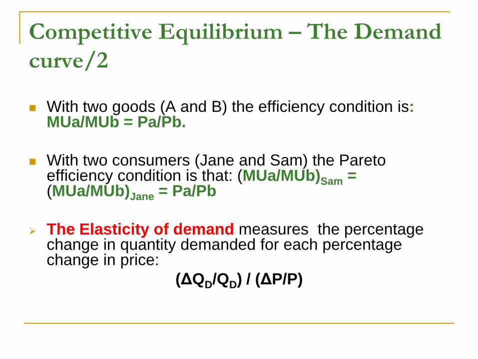
With two goods (A and B) the efficiency condition is: MUa/MUb = Pa/Pb.

With two consumers (Jane and Sam) the Pareto efficiency condition is that: (MUa/MUb)Sam = (MUa/MUb)Jane = Pa/Pb

The Elasticity of demand measures the percentage change in quantity demanded for each percentage change in price:

(ΔQD/QD) / (ΔP/P)

The equilibrium in perfect competition

Sa shows the quantity of good A firms are willing to supply at each price Pa

Da shows the quantity of good A consumers are willing to purchase at each price.

At the competitive equilibrium:

i. the marginal costs of producing good A for producers equals the price (on the Supply curve)

ii. the marginal Utility of acquiring good A for consumers equals the price (on the Demand curve),

Hence: MUa = MCa = Pa

which is the condition required for economic efficiency.

This partial equilibrium condition is

generalised (general equilibrium) by the profit

maximising behaviour of firms and the utility

maximising behaviour of consumers in

competitive markets.

With two goods and two consumers the

Pareto Efficiency conditions is:

(MUa/MUb) = MCa /MCb= MRTab= Pa/Pb;

with MUa/MUb equal for the two consumers.

Pa

Qa

Da

Sa

Measuring social efficiency/1

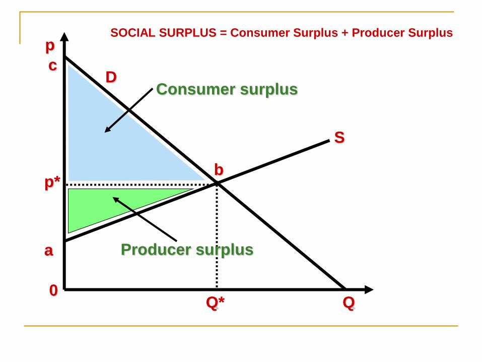
CONSUMER SURPLUS (CS): is the area below the demand curve and above the equilibrium market price, i.e. the difference between what consumers are willing to pay and what they have actually to pay. It measures the benefit consumers derive from consuming a good above and beyond the price they pay for that good.

WILLINGNESS TO PAY: how much a person is willing to pay in order to get additional units of a commodity. It measures the additional unit of utility the individual gets out of each additional unit of a commodity.

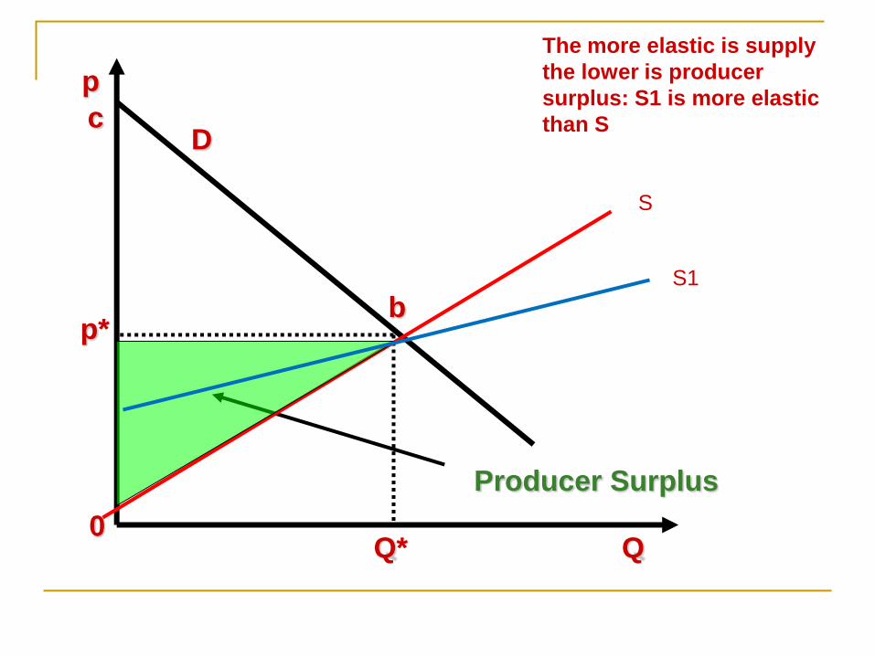
PRODUCER SURPLUS (PS): is the area below the equilibrium market price and above the supply curve. It measures the benefit (profits) the producers derive from selling a good, above and beyond the costs of producing that good.

SOCIAL SURPLUS OR SOCIAL EFFICIENCY:

PS+CS

The size of PS and CS depend on the elasticiy of supply and demand

0 Q

p

D

b p*

c

Q*

Consumer Surplus

S

The more elastic is

consumer demand the lower

is consumer surplus: D1 is

more elastic than D.

D1

0 Q

p

D

b p*

c

Q*

Producer Surplus

S

The more elastic is supply

the lower is producer

surplus: S1 is more elastic

than S

S1

0 Q

p

D

S

a

b p*

c

Q*

Consumer surplus

Producer surplus

SOCIAL SURPLUS = Consumer Surplus + Producer Surplus

0 Q

p

D

S

a

b p*

c

Q*

Consumer surplus:

Producer surplus:

from D+E to D+B

p1

Q1

A

B C

D E

from A + B + C

to A Welfare loss

C + E

Welfare loss (deadweight loss): reduction in social efficiency when

markets are not competitive: i.e. when the price p1 is higher than the

perfectly competitive price p*

0 Q

p

D

S

a

E p*

c

Q*

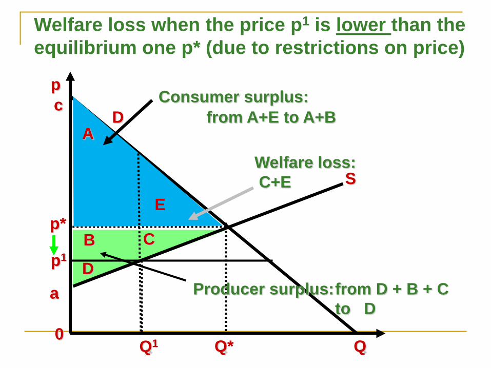
Consumer surplus:

Producer surplus:

p1

Q1

A

B C

D

Welfare loss:

C+E

from A+E to A+B

from D + B + C

to D

Welfare loss when the price p1 is lower than the

equilibrium one p* (due to restrictions on price)

E

Pareto efficiency and distribution of income: assumptions and limits

Behind the Pareto efficiency conditions there are a number of assumption:

The welfare of society is the sum of the welfares of all individuals in it;

Welfare is a private phenomenon: each individual is the best judge of his/her own welfare and of the choice of activities to reach it

Individuals are rational in pursuing the maximization of their welfare

Thus voluntary exchange is the only way to pursue social welfare and allocate resources and there must be unanimity in agreeing any socio-economic change.

Note that the PE condition accepts whatever distribution of income arises out of the free market system and derives the first best efficiency situation from it.

There are infinite configurations which satisfy PE, which depend on the initial endowments of individuals.

Pareto efficiency and distribution of income: assumptions and limits

Limits of PE:

Equity issues are disregarded by efficiency prescriptions.

There may be social values and interests which are not simply the sum of individual ones

individuals are not always able to act in their interests

Lump sum transfers among individuals (as required by the 2° theorem) are not always feasible.