20-1 cost-volume profit analysis prepared by douglas cloud pepperdine university prepared by douglas...
TRANSCRIPT

20-1
Cost-Cost-Volume Volume Profit Profit
AnalysisAnalysisPrepared by
Douglas Cloud Pepperdine University
Prepared by Douglas Cloud
Pepperdine University

20-2
1. Determine the number of units that must be sold to break even or to earn a targeted profit.
2. Calculate the amount of revenue required to break even or to earn a targeted profit.
3. Apply cost-volume-profit analysis in a multiple-product setting.
4. Prepare a profit-volume graph and a cost-volume-profit graph, and explain the meaning of each.
ObjectivesObjectivesObjectivesObjectives
After studying this After studying this chapter, you should chapter, you should
be able to:be able to:
After studying this After studying this chapter, you should chapter, you should
be able to:be able to:
ContinuedContinuedContinuedContinued
20-3
5. Explain the impact of the risk, uncertainty, and changing variables on cost-volume-profit analysis.
6. Discuss the impact of activity-based costing on cost-volume-profit analysis.
ObjectivesObjectivesObjectivesObjectives

20-4
Operating-Income ApproachOperating-Income ApproachOperating-Income ApproachOperating-Income Approach
Narrative Equation
Sales revenues
– Variable expenses
– Fixed expenses
= Operating income

20-5
Sales (72,500 units @ $40)
$2,900,000
Less: Variable expenses
1,740,000
Contribution margin
$1,160,000
Less: Fixed expenses
800,000
Operating income
$ 360,000
Operating-Income ApproachOperating-Income ApproachOperating-Income ApproachOperating-Income Approach
20-6
Operating-Income ApproachOperating-Income ApproachOperating-Income ApproachOperating-Income Approach
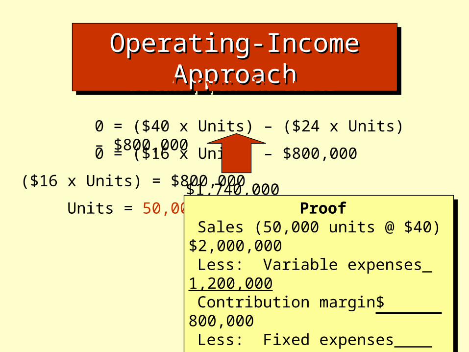
0 = ($40 x Units) – ($24 x Units) – $800,000
Break Even in Units
0 = ($16 x Units) – $800,000
($16 x Units) = $800,000
Units = 50,000 $1,740,000 ÷
72,500 ProofSales (50,000 units @ $40) $2,000,000Less: Variable expenses 1,200,000Contribution margin $ 800,000Less: Fixed expenses 800,000 Operating income $ 0
ProofSales (50,000 units @ $40) $2,000,000Less: Variable expenses 1,200,000Contribution margin $ 800,000Less: Fixed expenses 800,000 Operating income $ 0

20-7
Contribution-Margin ApproachContribution-Margin ApproachContribution-Margin ApproachContribution-Margin Approach
Number of units =
$800,000
$40 – $24
Number of units =
Number of units = 50,000 units
Fixed costs
Unit contribution margin

20-8
Target Income as a Dollar AmountTarget Income as a Dollar AmountTarget Income as a Dollar AmountTarget Income as a Dollar Amount
$424,000 = ($40 x Units) – ($24 x Units) – $800,000
$1,224,000 = $16 x Units
Units = 76,500
ProofSales (76,500 units @ $40) $3,060,000Less: Variable expenses 1,836,000Contribution margin $1,224,000Less: Fixed expenses 800,000 Operating income $ 424,000
ProofSales (76,500 units @ $40) $3,060,000Less: Variable expenses 1,836,000Contribution margin $1,224,000Less: Fixed expenses 800,000 Operating income $ 424,000

20-9
Target Income as a Percentage Target Income as a Percentage of Sales Revenueof Sales Revenue
Target Income as a Percentage Target Income as a Percentage of Sales Revenueof Sales Revenue
0.15($40)(Units) = ($40 x Units) – ($24 x Units) – $800,000
$6 x Units = ($40 x Units) – ($24 x Units) – $800,000
$6 x Units = ($16 x Units) – $800,000
$10 x Units = $800,000
Units = 80,000
More-Power Company wants to know the number of sanders that must be sold in order to earn a profit
equal to 15 percent of sales revenue.

20-10
Net income = Operating income – Income taxes
= Operating income – (Tax rate x Operating income)
After-Tax Profit TargetsAfter-Tax Profit TargetsAfter-Tax Profit TargetsAfter-Tax Profit Targets
= Operating income (1 – Tax rate)
Or
Operating income =Net income
(1 – Tax rate)

20-11
$487,500 = Operating income – 0.35(Operating income)
$487,500 = 0.65(Operating income)
After-Tax Profit TargetsAfter-Tax Profit TargetsAfter-Tax Profit TargetsAfter-Tax Profit Targets
$750,000 = Operating income
More-Power Company wants to achieve net income of $487,500 and its income tax rate is 35 percent.
Units = ($800,000 + $750,000)/$16Units = $1,550,000/$16Units = 96,875

20-12
After-Tax Profit TargetsAfter-Tax Profit TargetsAfter-Tax Profit TargetsAfter-Tax Profit Targets
ProofSales (96,875 units @ $40) $3,875,000Less: Variable expenses 2,325,000Contribution margin $1,550,000Less: Fixed expenses 800,000Income before income taxes $ 750,000Less: Income taxes (35%) 262,500 Net income $ 487,500
ProofSales (96,875 units @ $40) $3,875,000Less: Variable expenses 2,325,000Contribution margin $1,550,000Less: Fixed expenses 800,000Income before income taxes $ 750,000Less: Income taxes (35%) 262,500 Net income $ 487,500

20-13
Break-Even Point in Sales DollarsBreak-Even Point in Sales DollarsBreak-Even Point in Sales DollarsBreak-Even Point in Sales Dollars
Revenue Equal to Variable Cost Plus Contribution Margin
Contribution Contribution MarginMargin
$10
$6
$0
Variable CostVariable Cost
Revenue
10 Units
20-14
Break-Even Point in Sales DollarsBreak-Even Point in Sales DollarsBreak-Even Point in Sales DollarsBreak-Even Point in Sales Dollars
The following More-Power Company contribution margin income statement is
shown for sales of 72,500 sanders.
The following More-Power Company contribution margin income statement is
shown for sales of 72,500 sanders.
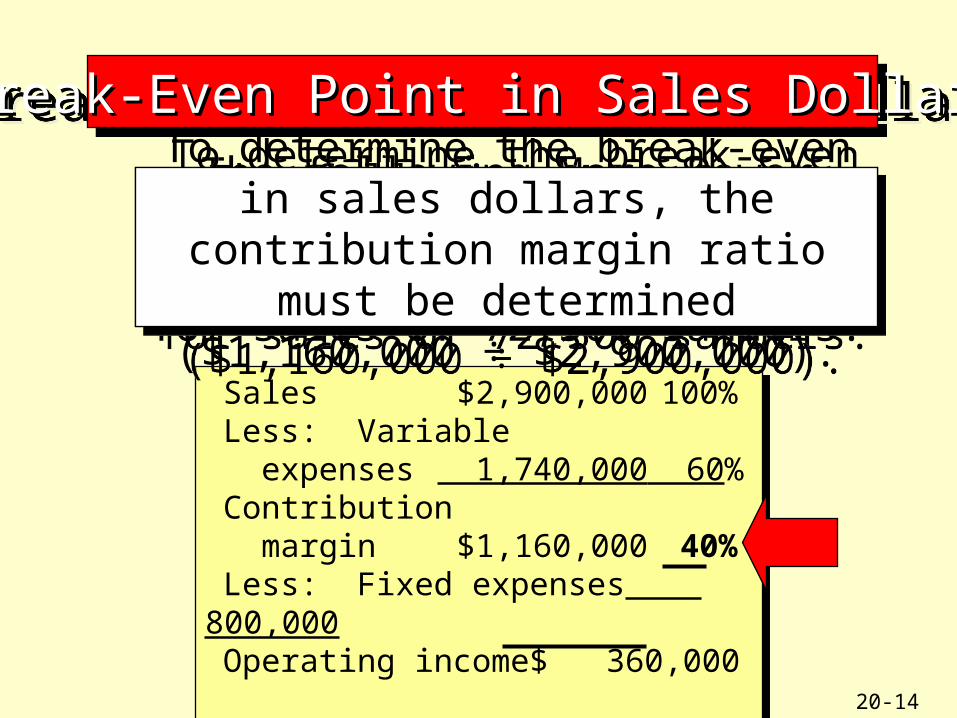
Sales $2,900,000 100%Less: Variable expenses 1,740,000 60%Contribution margin $1,160,000 40%Less: Fixed expenses 800,000Operating income $ 360,000
Sales $2,900,000 100%Less: Variable expenses 1,740,000 60%Contribution margin $1,160,000 40%Less: Fixed expenses 800,000Operating income $ 360,000
To determine the break-even in sales dollars, the contribution margin ratio must be determined ($1,160,000 ÷
$2,900,000).
To determine the break-even in sales dollars, the contribution margin ratio must be determined ($1,160,000 ÷
$2,900,000).
20-15
Break-Even Point in Sales DollarsBreak-Even Point in Sales DollarsBreak-Even Point in Sales DollarsBreak-Even Point in Sales Dollars
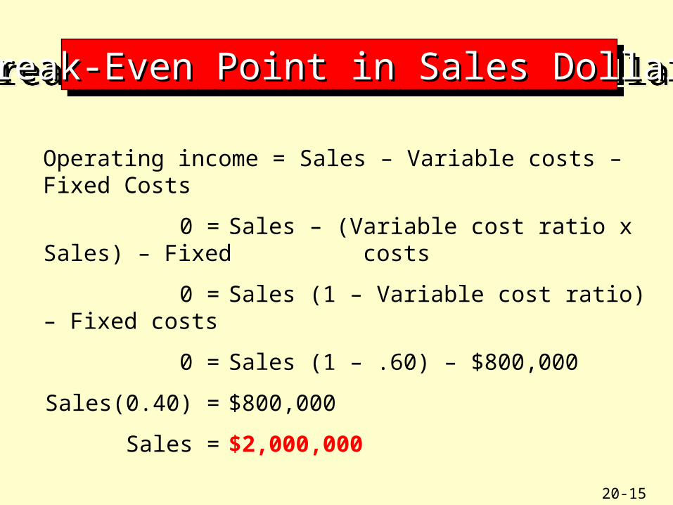
Operating income = Sales – Variable costs – Fixed Costs
0 = Sales – (Variable cost ratio x Sales) – Fixed costs
0 = Sales (1 – Variable cost ratio) – Fixed costs
0 = Sales (1 – .60) – $800,000
Sales(0.40) = $800,000
Sales = $2,000,000

20-16
Impact of Fixed Costs on ProfitsImpact of Fixed Costs on ProfitsImpact of Fixed Costs on ProfitsImpact of Fixed Costs on Profits
Fixed CostFixed Cost
Fixed Costs = Contribution Margin; Profit = 0
Contribution MarginContribution Margin
Total Variable CostTotal Variable Cost
Revenue

20-17
Impact of Fixed Costs on ProfitsImpact of Fixed Costs on ProfitsImpact of Fixed Costs on ProfitsImpact of Fixed Costs on Profits
Contribution MarginContribution Margin
Total Variable CostTotal Variable Cost
Revenue
Fixed CostFixed Cost
Fixed Costs < Contribution Margin; Profit > 0
ProfitProfit

20-18
Impact of Fixed Costs on ProfitsImpact of Fixed Costs on ProfitsImpact of Fixed Costs on ProfitsImpact of Fixed Costs on Profits
Contribution MarginContribution Margin
Total Variable CostTotal Variable Cost
Revenue
Fixed CostFixed Cost
Fixed Costs > Contribution Margin; Profit < 0
LossLoss

20-19
Profit TargetsProfit TargetsProfit TargetsProfit Targets
How much sales revenue must More-Power generate to earn a before-tax profit of $424,000?
Sales = ($800,000) + $424,000/0.40
= $1,224,000/0.40
= $3,060,000

20-20
Multiple-Product AnalysisMultiple-Product AnalysisMultiple-Product AnalysisMultiple-Product Analysis
Regular Mini- Sander Sander Total
Sales $3,000,000 $1,800,000 $4,800,000Less: Variable expenses 1,800,000 900,000 2,700,000
Contribution margin $1,200,000 $ 900,000 $2,100,000Less: Direct fixed expenses 250,000 450,000 700,000
Product margin $ 950,000 $ 450,000 $1,400,000Less: Common fixed exp. 600,000
Operating income $ 800,000

20-21
Multiple-Product AnalysisMultiple-Product AnalysisMultiple-Product AnalysisMultiple-Product Analysis
Regular sander break-even units
= Fixed costs/(Price – Unit variable cost)
= $250,000/$16
= 15,625 units
Mini-sander break-even units
= Fixed costs/(Price – Unit variable cost)
= $450,000/$30
= 15,000 units
20-22
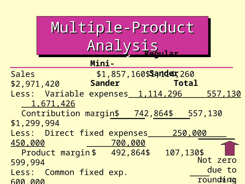
Multiple-Product AnalysisMultiple-Product AnalysisMultiple-Product AnalysisMultiple-Product Analysis
Regular Mini- Sander Sander Total
Sales $1,857,160 $1,114,260 $2,971,420Less: Variable expenses 1,114,296 557,130 1,671,426
Contribution margin $ 742,864 $ 557,130 $1,299,994Less: Direct fixed expenses 250,000 450,000 700,000
Product margin $ 492,864 $ 107,130 $ 599,994Less: Common fixed exp. 600,000
Operating income $ -6
Not zero due to rounding

20-23
Profit-Volume Graph
Profit or Loss
Loss
(40, $100)I = $5X - $100
Break-Even Point(20, $0)
$100—
80—
60—
40—
20—
0—
- 20—
- 40—
-60—
-80—
-100—
5 10 15 20 25 30 35 40 45 50 | | | | | | | | | |
Units Sold
(0, -$100)
20-24
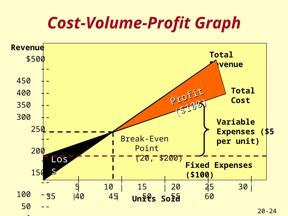
Cost-Volume-Profit GraphRevenue
Units Sold
$500 --
450 --
400 --
350 --
300 --
250 --
200 --
150 --
100 --
50 --
0 -- 5 10 15 20 25 30 35 40 45 50 55 60 | | | | | | | | | | | |
Total Revenue
Total Cost
Profit ($100)
Profit ($100)
LossLoss
Break-Even Point (20, $200)
Fixed Expenses ($100)
Variable Expenses ($5 per unit)

20-25
Assumptions of C-V-P AnalysisAssumptions of C-V-P AnalysisAssumptions of C-V-P AnalysisAssumptions of C-V-P Analysis
1. The analysis assumes a linear revenue function and a linear cost function.
2. The analysis assumes that price, total fixed costs, and unit variable costs can be accurately identified and remain constant over the relevant range.
3. The analysis assumes that what is produced is sold.
4. For multiple-product analysis, the sales mix is assumed to be known.
5. The selling price and costs are assumed to be known with certainty.

20-26
$
Units
Total Cost
Total Revenue
Relevant Range
Relevant Range

20-27
Alternative 1: If advertising expenditures increase by $48,000, sales will increase from 72,500 units to 75,000 units.
Before theBefore the With theWith the IncreasedIncreased IncreasedIncreased
AdvertisingAdvertising AdvertisingAdvertising
Units sold 72,500 75,000Unit contribution margin x $16 x $16Total contribution margin $1,160,000 $1,200,000Less: Fixed expenses 800,000 848,000 Profit $ 360,000 $ 352,000
Difference in ProfitsDifference in Profits
Change in sales volume 2,500Unit contribution margin x $16
Change in contribution margin $40,000Less: Increase in fixed expense 48,000 Decrease in profit $ -8,000

20-28
Before the Before the With theWith theProposed Proposed ProposedProposed
Price IncreasePrice Increase Price IncreasePrice IncreaseUnits sold 72,500 80,000Unit contribution margin x $16 x $16
Total contribution margin $1,160,000 $1,120,000Less: Fixed expenses 800,000 800,000 Profit $ 360,000 $ 320,000
Alternative 2: A price decrease from $40 per sander to $38 would increase sales from 72,500 units to 80,000 units.
Difference in Difference in ProfitProfit
Change in contribution margin $-40,000Less: Change in fixed expenses ----- Decrease in profit $-40,000
20-29
Before theBefore the With the ProposedWith the ProposedProposed Price andProposed Price and Price DecreasePrice Decrease
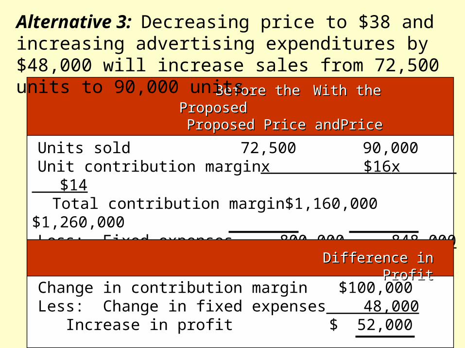
Advertising ChangeAdvertising Change Advertising Advertising IncreaseIncreaseUnits sold 72,500 90,000
Unit contribution margin x $16 x $14Total contribution margin $1,160,000 $1,260,000
Less: Fixed expenses 800,000 848,000 Profit $ 360,000 $ 412,000
Alternative 3: Decreasing price to $38 and increasing advertising expenditures by $48,000 will increase sales from 72,500 units to 90,000 units.
Difference in ProfitDifference in Profit
Change in contribution margin $100,000Less: Change in fixed expenses 48,000 Increase in profit $ 52,000

20-30
Margin of SafetyMargin of SafetyMargin of SafetyMargin of Safety
Assume that a company has a break-even volume of 200 units and the company is currently selling 500 units.
Current sales 500Break-even volume 200Margin of safety (in units) 300
Break-even point in dollars: Current revenue
$350,000Break-even volume
200,000Margin of safety (in dollars)
$150,000

20-31
Operating LeverageOperating LeverageAutomated Manual
System SystemSales (10,000 units) $1,000,000 $1,000,000Less: Variable expenses 500,000 800,000
Contribution margin $ 500,000 $ 200,000Less: Fixed expenses 375,000 100,000
Operating income $ 125,000 $ 100,000
Unit selling price $100 $100Unit variable cost 50 80Unit contribution margin 50 20
$500,000 ÷ $125,000 = DOL of 4
$500,000 ÷ $125,000 = DOL of 4
$200,000 ÷ $200,000 = DOL of 2
$200,000 ÷ $200,000 = DOL of 2
20-32
Operating LeverageOperating Leverage
What happens to profit in each system if sales increase by 40 percent?
What happens to profit in each system if sales increase by 40 percent?

20-33
Operating LeverageOperating LeverageAutomated Manual
System SystemSales (14,000 units) $1,400,000 $1,400,000Less: Variable expenses 700,000 1,120,000
Contribution margin $ 700,000 $ 280,000Less: Fixed expenses 375,000 100,000
Operating income $ 325,000 $ 180,000
Automated system—40% x 4 = 160%$125,000 x 160% =
$200,000 increase$125,000 + $200,000 =
$325,000
Manual system—40% x 2 = 80%$100,000 x 80% = $80,000 $100,000 + $80,000 =
$180,000

20-34
CVP Analysis and ABCCVP Analysis and ABCCVP Analysis and ABCCVP Analysis and ABC
Total cost = Fixed costs + (Unit variable cost x Number of units) + (Setup cost x Number of setups) + (Engineering cost x Number of engineering hours)
The ABC Cost Equation
Operating income = Total revenue – [Fixed costs + (Unit variable cost x Number of units) + (Setup cost x Number of setups) + (Engineering cost x Number of engineering hours)]
Operating Income

20-35
CVP Analysis and ABCCVP Analysis and ABCCVP Analysis and ABCCVP Analysis and ABC
Break-even units = [Fixed costs + (Setup cost x Number of setups) + (Engineering cost x Number of engineering hours)]/(Price – Unit variable cost)
Break-Even in Units
Differences Between ABC Break-Even and Convention Break-Even
The fixed costs differ
The numerator of the ABC break-even equation has two nonunit-variable cost terms

20-36
CVP Analysis and ABC—ExampleCVP Analysis and ABC—ExampleCVP Analysis and ABC—ExampleCVP Analysis and ABC—Example
Data about Variables
Cost Driver Unit Variable Cost Level of Cost DriverUnits sold $ 10 --
Setups 1,000 20
Engineering hours 30 1,000
Other data:
Total fixed costs (conventional)$100,000
Total fixed costs (ABC) 50,000
Unit selling price 20

20-37
CVP Analysis and ABC—ExampleCVP Analysis and ABC—ExampleCVP Analysis and ABC—ExampleCVP Analysis and ABC—Example
Units to be sold to earn a before-tax profit of $20,000:
Units = (Targeted income + Fixed costs)/(Price – Unit variable cost)
= ($20,000 + $100,000)/($20 – $10)
= $120,000/$10
= 12,000 units
20-38
CVP Analysis and ABC—ExampleCVP Analysis and ABC—ExampleCVP Analysis and ABC—ExampleCVP Analysis and ABC—Example
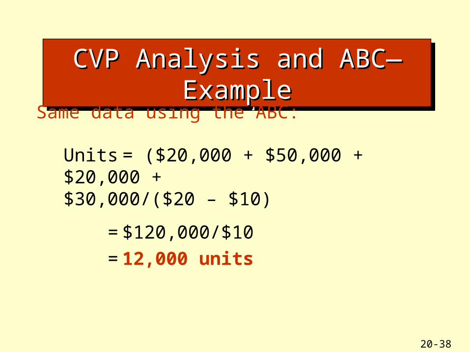
Same data using the ABC:
Units = ($20,000 + $50,000 + $20,000 + $30,000/($20 – $10)
= $120,000/$10
= 12,000 units

20-39
CVP Analysis and ABC—ExampleCVP Analysis and ABC—ExampleCVP Analysis and ABC—ExampleCVP Analysis and ABC—Example
Suppose that marketing indicates that only 10,000 units can be sold. A new design reduces direct labor by $2 (thus, the new variable cost is $8). The new break-even is calculated as follows:
Units = Fixed costs/(Price – Unit variable cost)
= $100,000/($20 – $8)
= 8,333 units

20-40
CVP Analysis and ABC—ExampleCVP Analysis and ABC—ExampleCVP Analysis and ABC—ExampleCVP Analysis and ABC—Example
The projected income if 10,000 units are sold is computed as follows:
Sales ($20 x 10,000) $200,000
Less: Variable expenses ($8 x10,000) 80,000
Contribution margin $120,000
Less: Fixed expenses 100,000
Operating income $ 20,000

20-41
CVP Analysis and ABC—ExampleCVP Analysis and ABC—ExampleCVP Analysis and ABC—ExampleCVP Analysis and ABC—Example
Suppose that the new design requires a more complex setup, increasing the cost per setup from $1,000 to $1,600. Also, suppose that the new design requires a 40 percent increase in engineering support. The new cost equation is given below:
Total cost = $50,000 + ($8 x Units) + ($1,600 x Setups) + ($30 x Engineering hours)
20-42
CVP Analysis and ABC—ExampleCVP Analysis and ABC—ExampleCVP Analysis and ABC—ExampleCVP Analysis and ABC—Example
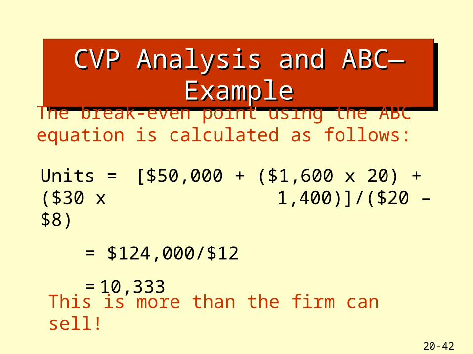
The break-even point using the ABC equation is calculated as follows:
Units = [$50,000 + ($1,600 x 20) + ($30 x 1,400)]/($20 – $8)
= $124,000/$12
= 10,333
This is more than the firm can sell!

20-43
End ofEnd of
ChapterChapter

20-44