1

2001-10 Rapid Design Iteration Process for Spacecraft Kinematic Mounts

Using Automatic Tet Meshing and Global/Local Modeling Techniques

Chris Luanglat TRW Space & Electronics

One Space Park Redondo Beach, CA 90278

(310) 812-9007 chris.luanglat@trw.com

and

Hanson Chang

MSC.Software Corporation 2 MacArthur Place

Santa Ana, CA 92707 (714) 445-5638

hanson.chang@mscsoftware.com

Abstract Spacecraft kinematic mounts have been successfully developed at TRW Space & Electronics to support instruments on the Aqua and Aura spacecrafts. Kinematic mounts are flexures which allow differential strains to develop between the spacecraft structure and the instruments without inducing significant load into the instruments. The kinematic mount designers and analysts are faced with the challenge of making multiple design iterations in a short amount of time. To meet this challenge, a rapid design iteration process has been developed using MSC.Patran and MSC.Nastran. This paper presents this rapid design iteration process. In particular, the direct import of CAD solid geometry, the extensive use of automatic tet meshing, and the application of global/local modeling techniques are presented.

2

1.0 INTRODUCTION 1.1 PROGRAM OVERVIEW TRW Space & Electronics is the prime contractor for the Aqua and Aura spacecraft which are part of the NASA Earth Observing System (EOS) program. These spacecraft will allow us to study and understand the atmosphere, the ocean, and the land surface of our home planet earth. The scheduled launch dates are 12/2001 for the Aqua spacecraft and 7/2003 for the Aura spacecraft. Aqua and Aura are state-of-the-art spacecraft constructed from advanced composite materials. These spacecrafts have an open-architecture configuration with the science instruments mounted on the outside of the primary structure. Shown in Figure 1 is the Aqua spacecraft in the launch stowed configuration. It measures 22 ft x 9ft x 8 ft and weighs 6,500 lbs. Figure 2 shows the spacecraft in the on-orbit deployed configuration.

Figure 1. The Aqua Spacecraft - Stowed Figure 2. The Aqua Spacecraft - Deployed

1.2 INSTRUMENT ATTACHMENT TO PRIMARY STRUCTURE The primary structure, which is the backbone of the spacecraft, provides the load path between the instruments and the launch vehicle during launch. It is designed for stiffness and strength to survive the launch environment. It must also retain dimensional stability on orbit so that the fine-pointing instruments can find their targets. A box-beam type primary structure design is used for both spacecraft. Figure 3 shows the MSC.Nastran finite element model of the overall Aqua spacecraft. The primary structure portion of the finite element model is shown in Figure 4.

3

Figure 3. The Aqua Spacecraft Finite Element Model

Figure 4. Primary Structure Finite Element Model

4

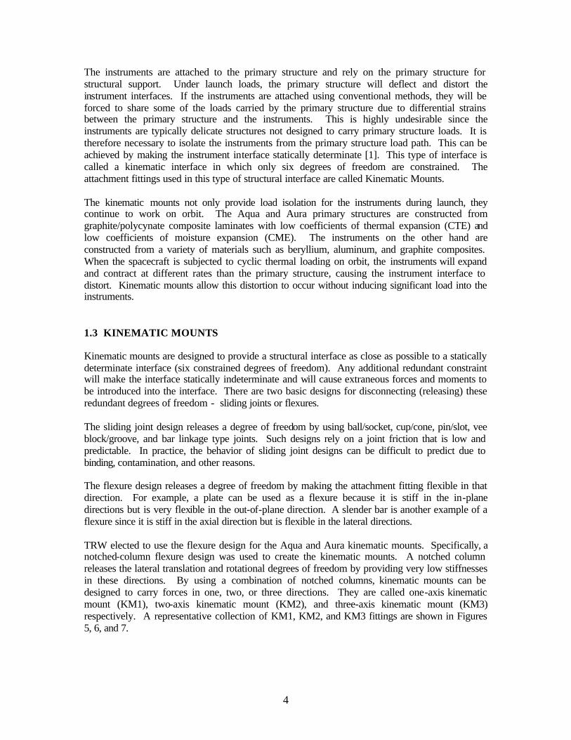
The instruments are attached to the primary structure and rely on the primary structure for structural support. Under launch loads, the primary structure will deflect and distort the instrument interfaces. If the instruments are attached using conventional methods, they will be forced to share some of the loads carried by the primary structure due to differential strains between the primary structure and the instruments. This is highly undesirable since the instruments are typically delicate structures not designed to carry primary structure loads. It is therefore necessary to isolate the instruments from the primary structure load path. This can be achieved by making the instrument interface statically determinate [1]. This type of interface is called a kinematic interface in which only six degrees of freedom are constrained. The attachment fittings used in this type of structural interface are called Kinematic Mounts. The kinematic mounts not only provide load isolation for the instruments during launch, they continue to work on orbit. The Aqua and Aura primary structures are constructed from graphite/polycynate composite laminates with low coefficients of thermal expansion (CTE) and low coefficients of moisture expansion (CME). The instruments on the other hand are constructed from a variety of materials such as beryllium, aluminum, and graphite composites. When the spacecraft is subjected to cyclic thermal loading on orbit, the instruments will expand and contract at different rates than the primary structure, causing the instrument interface to distort. Kinematic mounts allow this distortion to occur without inducing significant load into the instruments. 1.3 KINEMATIC MOUNTS Kinematic mounts are designed to provide a structural interface as close as possible to a statically determinate interface (six constrained degrees of freedom). Any additional redundant constraint will make the interface statically indeterminate and will cause extraneous forces and moments to be introduced into the interface. There are two basic designs for disconnecting (releasing) these redundant degrees of freedom - sliding joints or flexures. The sliding joint design releases a degree of freedom by using ball/socket, cup/cone, pin/slot, vee block/groove, and bar linkage type joints. Such designs rely on a joint friction that is low and predictable. In practice, the behavior of sliding joint designs can be difficult to predict due to binding, contamination, and other reasons. The flexure design releases a degree of freedom by making the attachment fitting flexible in that direction. For example, a plate can be used as a flexure because it is stiff in the in-plane directions but is very flexible in the out-of-plane direction. A slender bar is another example of a flexure since it is stiff in the axial direction but is flexible in the lateral directions. TRW elected to use the flexure design for the Aqua and Aura kinematic mounts. Specifically, a notched-column flexure design was used to create the kinematic mounts. A notched column releases the lateral translation and rotational degrees of freedom by providing very low stiffnesses in these directions. By using a combination of notched columns, kinematic mounts can be designed to carry forces in one, two, or three directions. They are called one-axis kinematic mount (KM1), two-axis kinematic mount (KM2), and three-axis kinematic mount (KM3) respectively. A representative collection of KM1, KM2, and KM3 fittings are shown in Figures 5, 6, and 7.

5

Figure 5. Representative Collection of KM1 Fittings

Figure 6. Representative Collection of KM2 Fittings

6

Figure 7. Representative Collection of KM3 Fittings

The simplest kinematic mount arrangement uses one KM1, one KM2, and one KM3 in a three-point attachment scheme. The MODIS instrument shown in Figure 8 is supported in this fashion. Other combinations of kinematic mounts are used throughout the two spacecraft.

Figure 8. The MODIS Instrument Supported on Three Kinematic Mounts

KM1

KM3

KM2

7

2.0 DESIGN CHALLENGES In today’s competitive market, products must be delivered on schedule, with high quality, and at a low cost. The prudent engineer is therefore constantly looking for ways to do his/her job faster, better, and cheaper. In the case of kinematic mounts, the TRW structures engineers looked for ways to shorten the development time for each kinematic mount at the onset of the program. Since a number of kinematic mounts were required for each spacecraft, the time savings could add up quickly. The lessons learned could also be passed on to other spacecraft programs using kinematic mounts to support instruments. The main challenge facing the structures engineers was the multiple design requirements the kinematic mounts must meet. The conventional secondary structure design requirements typically include strength, fatigue, stiffness, and size. An acceptable design must be strong enough to withstand launch loads (strength), be able to survive cyclic launch and on-orbit loads (fatigue), have a natural frequency higher than a target frequency (stiffness), and fit in the tight space between the instruments and the primary structure (size). The design which meets all these requirements is located in the solution space which is the intersection of the three design spaces as shown in Figure 9.

Figure 9. Conventional Secondary Structure Solution Space

In addition to the conventional secondary structure design requirements, the kinematic mounts must also meet several other requirements. One requirement is flexibility because the stiffnesses in the released directions must be low. Another requirement is stability because the notched columns can potentially buckle as Euler columns. One last requirement is fracture because the kinematic mounts are classified as fracture critical parts. Meeting all these requirements is not an easy task because the kinematic mount solution space is much smaller than the conventional secondary structure solution space as demonstrated in Figure 10.

8

Figure 10. Kinematic Mount Design Solution Space

In order to find the kinematic mount design solution, the structural analyses listed below must be performed: Type of Analysis Numerical Analysis Tool

1. Strength Finite element stress analysis (MSC.Nastran SOL 101) 2. Stiffness Normal modes analysis (MSC.Nastran SOL 103) 3. Flexibility Finite element stiffness analysis (MSC.Nastran SOL 101) 4. Stability Finite element buckling analysis (MSC.Nastran SOL 105) 5. Fracture Crack growth analysis (NASA/FLAGRO)

Table 1. Summary of Structural Analyses

A typical kinematic mount design will not pass all these analysis checks the first time. For example, the first set of analyses may indicate that the initial design does not meet the flexibility requirement. As a result, the part geometry is modified to make it more flexible. The part is analyzed again and found to be yielding in the notched area. The part is redesigned again and ready for the next analysis cycle. Several such iteration cycles may be required before an acceptable design solution is found. The kinematic mount design process is therefore an iterative process. The success of the design effort depends on how quickly these design iterations can be performed. 3.0 GEOMETRY All five types of analyses mentioned above have one thing in common – they all require a detailed finite element model capable of predicting accurate displacements and stresses. Since the typical kinematic mount is a three-dimensional highly-sculptured part, the finite element

9

model must accurately represent this part geometry. The first step in constructing the finite element model is therefore to obtain the part geometry from the CAD model. The primary CAD software used at TRW is CATIA. At the beginning of the program, a typical CATIA part was exported as an IGES file. The IGES file was then imported into SDRC/I-DEAS as surfaces. The surfaces were stitched together to form a solid which was then meshed to generate solid elements. The imported IGES geometry typically required extensive cleanup before a solid could be generated. This was a labor-intensive process and not suitable for multiple design iterations. Alternatively the solid geometry could be recreated in I-DEAS using the solid-modeling capability within I-DEAS. This was again time consuming and not suitable for a multiple design iteration environment. Looking for ways to speed up the geometry creation process, the structures engineers started to evaluate MSC.Patran. MSC.Patran is capable of importing a CATIA solid directly into MSC.Patran as a solid using the CATIA Direct access option. The CATIA solid geometry is first translated into an Express Neutral file. The Express Neutral file is then imported into MSC.Patran. The success rate of bringing CATIA solid geometry into MSC.Patran as solid geometry using this method was high (95+%). MSC.Patran was therefore selected as the finite element pre-processing tool for the kinematic mounts. The quality of the CAD solid geometry is important for subsequent meshing operations. For example, sliver surfaces and short edges can cause very small or highly distorted elements to be generated during meshing operations. The small elements can cause the model to become excessively large while the highly distorted elements can produce poor numerical results. The most efficient way to correct these problem areas is to clean up the geometry on the CAD side [2]. Better yet, the need to clean up geometry can be virtually eliminated if the problems were not created in the first place. To work toward this goal, conferences were held between the designers and analysts to discuss why clean geometry was needed and to establish common practices to eliminate problem geometry. 4.0 MESHING 4.1 HEX MESHING VS. TET MESHING Traditionally the eight-node hexahedron element (brick element) is the preferred solid element type for performing detailed stress analysis. It is capable of representing linearly-varying displacement and stress fields within the element. Due to their brick shape, hex elements can only be generated by meshing 5 or 6-sided solids (simple solids) or by sweeping quadrilateral plate elements. A typical solid imported from a CAD package cannot be directly hex meshed. It must be first partitioned into simple solids before it can be hex meshed. There are two ways to do this:

1. Break the solid into simple solids using planes or surfaces 2. Disassemble the solid into surfaces. Break the surfaces into 3 or 4-sided surfaces and

reassemble them into simple solids [3] These two methods are commonly called “manual methods” because they require planning, patience, and time [4]. It may take a skilled structural analyst several days to manually hex mesh a complex part. Many structural analysts prefer to use these manual methods because the payoff is often an aesthetically-looking solid mesh with well-shaped hex elements.

10

The notched regions of a typical kinematic mount is shown in Figure 11. This part obviously can not be directly hex meshed. In order to hex meshed it, the manual methods mentioned earlier had to be used to partition the solid into simple solids. Although the manual methods resulted in well-shaped hex elements which generated good stress results, they were too time consuming for the multiple design iteration technique the kinematic mounts require. What was needed was a meshing method which will produce a mesh in a more automated fashion. The meshing cycle time needed to be reduced from days to hours. The MSC.Patran automatic tet mesher was the solution.

Figure 11. Typical Kinematic Mount Notched Regions The MSC.Patran automatic tet mesher is capable of meshing a complex solid directly to generate tetrahedron elements. It is called an “automatic” mesher because complex solid geometries can be directly tet meshed without any prior geometry manipulation. The elements generate by this mesher are either 4-node or 10-node tetrahedron elements (TET4 or TET10 elements). The TET4 element is a constant-strain element and is not suitable for capturing the high stress gradients typically found in kinematic mounts. The TET10 element is a linear-strain element with basis functions that are complete through the quadratic terms [5,6]. It is capable of representing a linearly-varying stress field within the element. It has four corner nodes and 6 mid-side nodes. The mid-side nodes allow the TET10 element to have curved edges and faces which enable it to capture the curved part geometry with a quadratic fit. The TET10 elements were selected to model the kinematic mounts. 4.2 MESH DENSITY CONTROL The most critical areas in a kinematic mount are the notched portions of the fitting where steep stress gradients (stress concentrations) exist. These areas also provide the flexibility needed for the kinematic mount to flex. These areas are also where the initial flaws will be placed for crack growth analysis. The main goal of the finite element analysis is therefore to compute stiffness and stresses accurately in these critical areas. The key to accurately capturing the stiffness and stresses in these notched areas is to use a fine solid mesh. Since these critical areas make up only a small percentage of the overall fitting volume, the rest of the fitting should be meshed with a coarser mesh in order to keep the size of the finite element model reasonable. The transition from fine mesh to coarse mesh should occur

Notched Regions

11

outside the critical areas. This can be achieved by breaking the solid into multiple solids using a “cookie cutter” approach as shown in Figures 12, 13, and 14. The solid in each case is broken up using the plane or surface option in MSC.Patran. This approach isolates the critical area from the rest of the part. Mesh the critical solid first with a small element size. Next mesh the surrounding solids with larger element sizes. MSC.Patran automatically makes the mesh transition from fine mesh to coarse mesh in these surrounding solids.

Figure 12. Mesh Density Control Example 1

Figure 13. Mesh Density Control Example 2

Figure 14. Mesh Density Control Example 3

12

The cookie-cutter method is a very efficient way of placing a large number of elements in the right place and allows for transitioning to a coarser mesh automatically. Further mesh control in the critical areas can be achieved by surface meshing the solid faces first with TRIA6 elements to guide subsequent tet meshing. The kinematic mount model sizes ranged from 100,000 DOF for the simpler KM1 fittings to 750,000 DOF for the more complex KM3 fittings. The average time it took to automatic tet mesh a kinematic mount was about 2 hours (using IBM RS6000-43P workstations) which was much faster than the conventional hex meshing technique which typically required several days to mesh the same part. The shortened meshing time made it possible to go through multiple design iterations and evaluate various design options in a timely fashion. 4.3 MULTI-PASS CONVERGENCE VS. SINGLE-PASS CONVERGENCE In order to accurately capture the highest stresses in a kinematic mount, the TET10 mesh must be fine enough in the notched areas of the fitting. There must be enough elements through the thickness of the part to capture the steep stress gradients in these areas. There are two ways to determine the number of elements required through the thickness – the multi-pass convergence method and the single-pass convergence method. In the multi-pass convergence method, the user makes multiple analysis runs with increasing mesh density. The highest part stress is recorded for each run and compared against the previous run. Convergence is reached when the percent change in stress between two runs falls below a certain number, such as 5%. When convergence is reached, it is an indication that the number of elements through the part thickness is adequate to capture the stress gradient. In the single-pass convergence method, the user meshes the part once and runs the analysis. The stress results from this single run are evaluated based on how large the stress discontinuities are. This is done in MSC.Patran by making stress fringe plots using the “difference” option. MSC.Patran examines the stress results from elements sharing a common node and computes the difference between the maximum and minimum stresses. These stress differences (discontinuities) are plotted for all the nodes in the model. Large stress discontinuities indicate that the mesh is too coarse. Small stress discontinuities indicate that the mesh density is adequate [7]. A combination of these two convergence methods were used for the kinematic mounts. For each type of notch geometry (circular, square, rectangular, etc.), the multi-pass convergence test is performed first to determine the number of elements required through the thickness of the part. For subsequent design iterations, the part is meshed only once per iteration using the meshing guidelines established by the multi-pass convergence test. Stress discontinuity plots are used to verify the quality of the mesh. 5.0 GLOBAL/LOCAL MODELING TECHNIQUES The Aqua spacecraft finite element model shown in Figure 3 is a 250,000 DOF model, not including the kinematic mounts. The size of the kinematic mount detailed solid element models range from 100,000 DOF to 750,000 DOF each. If several dozens of these kinematic mounts were directly integrated into the spacecraft model, it would make the spacecraft model

13

unacceptably large. A global/local modeling approach was needed to integrate the kinematic mounts into the spacecraft model. There are two ways to mathematically reduce the kinematic mounts – Static Reduction (Guyan Reduction) and Dynamic Reduction. The Static Reduction method uses Guyan reduction to reduce a kinematic mount to a stiffness matrix and a mass matrix. This method ignores the dynamic effects internal to the kinematic mount. The Dynamic Reduction method captures the dynamic effects internal to the kinematic mount by using Component Modal Synthesis. Since kinematic mounts are compact fittings with natural frequencies much higher than the spacecraft structure natural frequencies, the kinematic mount internal dynamic effects can be ignored. Static Reduction was therefore used to reduce the kinematic mounts. Using Static Reduction, each kinematic mount is reduced to a small set of DOF representing the boundary of the fitting. Each interface region in a fitting is first wagon-wheeled to a single boundary node using an RBE2. For example, the KM2 fitting shown in Figure 15 is wagon-wheeled to three boundary nodes. The kinematic mount model (25,000 DOF) is next reduced to a stiffness matrix (18 x 18) and a mass matrix (18 x 18) using the three boundary nodes. The reduction process requires two entries in the bulk data section [8]:

1. ASET entry which specifies the boundary DOF 2. PARAM, EXTOUT, DMIGPCH entry which extracts and writes the reduced matrices to

the punch file in DMIG format Once the reduction process is complete, the reduced matrices are written to a punch file. The punch files containing the reduced matrices for all the kinematic mounts are next merged into one file and inserted into the spacecraft bulk data section using the include statement. In the case control section, the K2GG and M2GG entries are used to assemble the reduced matrices into the spacecraft model stiffness and mass matrices.

Figure 15. Interface Regions Wagon-Wheeled Figure 16. Enforced Displacements to Boundary Nodes Applied to Boundary Nodes The global spacecraft model is now ready for the next load cycle. This model is used in the coupled-loads analysis to compute launch accelerations for the spacecraft components. The resulting accelerations are converted to design load factors and are applied to the global model to generate internal loads and displacements for the spacecraft components. For the kinematic mounts, the interface displacement results are recovered at the kinematic mount boundary nodes

14

and converted to enforced displacement SPCD entries using the MSC.Patran FEM Field option. The enforced displacements are next applied to the kinematic mount detailed solid element models as shown in Figure 16 to start a new design cycle. 6.0 CONCLUSIONS A rapid design iteration process was developed for spacecraft kinematic mounts at TRW. This process involved three key steps:

1. Direct CAD geometry access 2. Automatic tet meshing with single pass convergence 3. Global/local modeling using static reduction

The rapid design iteration process resulted in substantial cycle time reduction for the Aqua and Aura spacecraft kinematic mounts. The kinematic mounts for the Aqua spacecraft have successfully passed the full spacecraft vibration test shown in Figure 17. The notched-column kinematic mount design configurations have been incorporated into the TRW Deployables Handbook. It is expected that the rapid design iteration process presented in this paper will benefit TRW engineers and other MSC.Software product users facing similar design challenges in the future.

Figure 17. The Aqua Spacecraft Undergoing Vibration Testing

15

7.0 ACKNOWLEDGMENTS The authors express their gratitude to Mr. Garrett Wittkopp of TRW Space & Electronics for his helpful suggestions and guidance throughout the Aqua and Aura spacecraft programs. 8.0 REFERENCES [1] Sarafin, T. P., Spacecraft Structures and Mechanisms - From Concept to Launch,

Microcosm Press, 1995, pp. 514-516 [2] McKenney, D., “Model Quality: The Key to CAD/CAM/CAE Interoperability”, MSC

Americas Users’ Conference Proceedings, 1998 [3] Soeiro, A., “SNECMA Blade and Disk Meshing Methodology”, MSC Worldwide

Aerospace Conference Proceedings, Vol. 1 , 1999. [4] Adams, V. and Abraham, A., Building better Products with Finite Element Analysis, 1st

ed., OnWord Press, 1999, pp. 249-251 [5] MacNeal, R. H., Finite Elements: Their Design and Performance, Marcel Dekker, 1994,

pp. 75, 88 [6] Cook, R. D., Finite Element Modeling for Stress Analysis, John Wiley & Sons, 1995, pp.

150 [7] NAFEMS, A Finite Element Primer, Birniehill, Glasgow, 1992, pp. 158-160 [8] Rose, T., “The New External Superelements in MSC/NASTRAN and a DMAP Alter to

Create and Use OTM”, MSC Worldwide Aerospace Conference Proceedings, Vol. 1, 1999