1

2005 Stock Status of Cowcod in the Southern California Bight

and Future Prospects

May 25th 2005

Kevin Piner SWFSC

8604 La Jolla Shores Drive, La Jolla Ca. 92037

Edward J. Dick and

John Field SWFSC

110 Shaffer Rd. Santa Cruz, CA. 95060

2

Table of Contents Document Section pg Executive Summary 3 Introduction 10 Section 1. Biology Fisheries and Data 11 Section 2. Assessment 24 Literature Cited 28 Tables 34 Figures 48 Appendix I Delay Difference Model 60 Appendix II GMT Tables 69 Appendix III Data and Control Files 70 Appendix IV Expansion of Visual estimate using CPFV 79 Appendix V Expansion of Visual estimate using CalCOFI 93 Appendix VI numbers at age 125

3

Executive Summary Stock. Cowcod (Sebastes levis) in the Southern California Bight (SCB) is the “stock” described by the modeling. The SCB is at the southern end of the INPFC Conception management area and extends from the US-Mexio border north to Point Conception at about 34o 30' N. Lat. Areas to the north and south of SCB were not included in the first assessment because of lack of data and possible differences in abundance trends. The SCB is the area where cowcod are most abundant, where adult habitat is most common and where catches are highest. Although larvae may spread across larger distances, we assume that the adults do not move beyond the stock boundary. This assumption, however, is untested and may very well be inaccurate. Catches Catches in this assessment were a combination of commercial and recreational fleets. Commercial catches were taken from the CALCOM database and recreational catches from the RecFIN database. The commercial fishery was made up primarily of set net gears, and to a lesser extent hook and line gears. The limited biological samples indicated commercial gears catch larger fish than recreational. Catches since 2001 have been very low due to management action, however catches in the 1980’s were substantially higher. Discard is not assumed except for a minimal discard in the years after the no-retention management. Table of catches (1995-2005)

Year Commercial catch (t) Recreational catch (t) Total (t) 1995.0 23.3 1.7 25.0 1996.0 24.6 5.4 30.0 1997.0 7.3 1.8 9.0 1998.0 1.2 2.8 4.0 1999.0 3.5 3.8 7.0 2000.0 0.4 4.5 5.0 2001.0 <1 <1 0.5 2002.0 <1 <1 0.5 2003.0 <1 <1 0.5 2004.0 <1 <1 0.5 2005.0 <1 <1 0.5

year

1920 1940 1960 1980 2000

catc

h (t)

50

100

150

200

250

Figure of catch by fleet. Dark bars represent commercial catch and light bars recreational.

4

Data and Assessment The last assessment of cowcod was completed in 1999. Data for this assessment include catch (1916-2005), CPFV recreational CPUE (1963-2000), and a single visual transect survey estimate (2002). The data were likelihood components in a Stock Synthesis (V 1.19) age-structured production model (Stock Reduction analysis). The assessment consists of 3 models that differ in the assumed steepness (h) of the Beverton and Holt Stock-Recruit relationship (h=0.4, 0.5, and 0.6). The models are not equally likely but range in probability from 30%, 40%, and 30% for h= 0.4, 0.5, and 0.6, respectively. Probabilities were assigned based upon expert opinion. Unresolved Problems and Uncertainties. The assessment suffers from a lack of quality and consistent data. The CPFV CPUE series ended in 2000 due to management actions, and a time series of relative abundance post 2000 is not currently available. Development of a quantitative measure of relative abundance is necessary to monitor this population. Both the steepness of the Beverton and Holt stock recruit relationship and the natural mortality rate are influential to the assessment and were assumed. The model with assumed h=0.5 was deemed the most likely by the review panel, although the actual h is not known. Reference Points The default PFMC harvest rate for rockfish is F50%SPR. The target spawning biomass is 40% of an unfished population. Species that are currently below 25% of an unfished state are overfished and catch rates above those specified by the F50%SPR are considered overfishing. Currently (2005), cowcod spawning biomass is estimated to be between 14-21% of the unfished state indicating that cowcod are overfished. Catches in the most recent years have been minimal indicating that harvest levels are not sufficient to be currently overfishing the stock. Table of Biological reference points

H=0.4 h=0.5 h=0.6

Unfished age-1+ biomass (t)

3250 3191 3151

Unfished spawning biomass (t)

3101 3045 3007

Unfished age-0 recruit 60.6 59.6 58.8

Spawning biomass (t) at 40% unfished

1240 1218 1202

Exploitation rate (%) at F50%SPR

.033 .033 .033

2005 spawning biomass (t)

443 542 642

5

Stock Biomass Spawning stock biomass is estimated to have declined from virgin estimates of 3101-3007 t (h=0.4-0.6, respectively) to 2005 estimates of 443-642 t (=0.4-0.6, respectively). A table of biomass for the last 10 years is given in the section Exploitation Status.

year

1900 1920 1940 1960 1980 2000 2020

spaw

ning

bio

mas

s (t)

0

500

1000

1500

2000

2500

3000

3500

h=0.4h=0.5 h=0.6

Figure of spawning stock biomass trajectory from all 3 models that used different levels of h. Recruitment. Because of the paucity of data, recruitment was modeled as the predicted from a specified stock recruit relationship. Only the level of virgin recruitment was estimated and the steepness of the relationship was fixed at 3 levels. Recruits in this constrained model are predicted to have increased in recent years. A table of biomass for the last 10 years is given in the section

year

1900 1920 1940 1960 1980 2000 2020

Rec

ruits

0

10

20

30

40

50

60

70

h=0.4h=0.5h=0.6

Figure of recruitment from all 3 models that used different assumed levels of h.

6

Exploitation Status Currently, cowcod spawning biomass is estimated to be between 14-21% of the unfished state indicating that cowcod are overfished. Catches in the most recent years have been minimal indicating that harvest levels are not sufficient to be overfishing the stock.

h=0.4

0.00E+00

5.00E-01

1.00E+00

1.50E+00

2.00E+00

2.50E+00

3.00E+00

0 0.5 1 1.5 2 2.5 3

spawnbiomass/40% spawn bio

harv

est r

ate/

F50

%SP

R ra

te

h=0.5

0.00E+00

5.00E-01

1.00E+00

1.50E+00

2.00E+00

2.50E+00

3.00E+00

0 0.5 1 1.5 2 2.5 3

spawn bio / 40% virgin spawn bio

h=0.6

0.00E+00

5.00E-01

1.00E+00

1.50E+00

2.00E+00

2.50E+00

3.00E+00

3.50E+00

0 0.5 1 1.5 2 2.5 3

spawn bio / 40% spawn bio

Figure of the ratio of harvest rate/F50%SPR rate vs spawning biomass/40% unfished spawning biomass.

7

Table of age1+biomass (t), spawning biomass (t), age-0 recruits, harvest rates (%) and depletion levels 1995-2005. Results are given for each level of assumed h.

h=0.4 h=0.5 h=0.6

year age 1+ Spawn recruit-0 Hrate dep age 1+ Spawn recruit-0 Hrate dep age 1+ Spawn recruit-0 Hrate dep1995 348 296 13.3 0.025 0.10 397 333 19.6 0.023 0.11 444 366 26.7 0.021 0.121996 350 304 13.6 0.029 0.10 405 346 20.2 0.026 0.11 457 385 27.5 0.023 0.131997 345 305 13.7 0.008 0.10 406 353 20.5 0.007 0.12 465 398 28.1 0.007 0.131998 359 323 14.4 0.003 0.10 426 378 21.5 0.003 0.12 492 428 29.4 0.003 0.141999 377 344 15.1 0.005 0.11 451 405 22.6 0.005 0.13 523 462 30.7 0.004 0.152000 392 359 15.7 0.004 0.12 472 426 23.5 0.003 0.14 551 490 31.7 0.003 0.162001 407 375 16.3 0.000 0.12 494 448 24.3 0.000 0.15 580 519 32.7 0.000 0.172002 426 394 16.9 0.000 0.13 520 473 25.2 0.000 0.16 613 550 33.7 0.000 0.182003 444 411 17.6 0.000 0.13 545 497 26.1 0.000 0.16 646 581 34.7 0.000 0.192004 461 428 18.1 0.000 0.14 569 520 26.9 0.000 0.17 678 612 35.6 0.000 0.202005 478 444 18.7 0.000 0.14 593 542 27.7 0.000 0.18 710 642 36.4 0.000 0.21

Management Performance Since 2001, cowcod have been managed as a no retention fishery in California. The ABC has been 5 t and OY 2.4 t. Recent catches have been < 1t, and indicate that management has been effective at reducing landings unless there has been significant unreported fishing mortality. We have no information on significant unreported catches. The closure of prime cowcod habitat to fishing methods likely to take cowcod is assumed to have effectively reduced non-targeted catch.

Table of management performance. ABC, OY and Catch are given in (t). year ABC OY Catch2001 5 2.4 <1 2002 5 2.4 <1 2003 5 2.4 <1

2004 5 2.4 <1 2005 5 2.1 <1

Regional Management The stock is presently assumed to be a Southern California Bight population. We do not know if the areas north or south of the stock area may constitute additional fish in that population. We have no basis to recommend management on a different regional basis.

8

Forecasts. Forecasts of OY catches (t) are given for all 3 levels of assumed S/R steepness. In each projection, catch in 2006 was assumed to be the same as 2005 catch. Table of projections of OY (40-10 adjusted catch), age-1 biomass and depletion levels

h=0.4 h=0.5 h=0.6

year Catch (t) age-1+ biomass depletion (t)

Catch (t) age-1+ biomass depletion (t)

Catch (t) age-1+ biomass depletion (t)

2007 7.3 509 0.15 12.2 640 0.19 17.0 773 0.23

2008 7.8 518 0.15 12.9 651 0.20 17.9 788 0.24

2009 8.2 525 0.16 13.5 661 0.20 18.7 802 0.24

2010 8.6 531 0.16 14.1 671 0.20 19.5 815 0.24

2011 9.0 537 0.16 14.7 680 0.20 20.2 828 0.25

2012 9.3 543 0.16 15.2 688 0.20 20.9 840 0.25

2013 9.7 548 0.16 15.6 696 0.21 21.6 852 0.25

2014 10.0 553 0.16 16.1 705 0.21 22.2 864 0.26

2015 10.2 558 0.16 16.5 713 0.21 22.7 875 0.26

2016 10.5 562 0.17 16.9 721 0.21 23.3 887 0.26

2017 10.7 567 0.17 17.3 729 0.22 23.8 898 0.27

9

Decision Table A decision table was constructed using the 3 levels of assumed steepness of the BH S/R relationship as different states of nature describing the resiliency of the population. The OY catch levels (40-10 adjusted) predicted for each state of nature were used as the catch in forecasting (2007-2016) age1+ biomass and depletion levels assuming those catches are taken in all 3 states of nature. Series in bold font show decreasing population abundance. Table of estimated age 1+ biomass and depletion levels.

State of nature: Catch used in the model with

Management options: Catch derived from: Year catch(t)

Low resilience H=0.4 Prob=0.3

Medium resilience H=0.5 Prob=0.4

High resilience H=0.6 Prob=0.3

2007 7.3 509 0.15 639 0.19 773 0.232008 7.8 518 0.15 655 0.20 798 0.242009 8.2 525 0.16 670 0.20 821 0.252010 8.6 531 0.16 685 0.21 845 0.252011 9.0 537 0.16 699 0.21 868 0.262012 9.3 543 0.16 713 0.21 891 0.272013 9.7 548 0.16 727 0.22 914 0.272014 10.0 553 0.16 741 0.22 936 0.282015 10.2 558 0.16 754 0.22 959 0.29

Low resilience H=0.4

2016 10.5 562 0.17 768 0.23 982 0.302007 12.2 509 0.15 640 0.19 773 0.232008 12.9 512 0.15 651 0.20 793 0.242009 13.5 515 0.15 661 0.20 812 0.242010 14.1 516 0.15 671 0.20 831 0.252011 14.7 517 0.15 680 0.20 849 0.252012 15.2 517 0.15 688 0.20 866 0.262013 15.6 517 0.15 696 0.21 883 0.262014 16.1 516 0.15 705 0.21 900 0.272015 16.5 516 0.15 713 0.21 918 0.27

Medium resilience H=0.5

2016 16.9 515 0.15 721 0.21 935 0.282007 17.0 509 0.15 639 0.19 773 0.232008 17.9 508 0.15 646 0.19 788 0.242009 18.7 505 0.15 651 0.19 802 0.242010 19.5 502 0.15 656 0.20 815 0.242011 20.2 497 0.15 659 0.20 828 0.252012 20.9 492 0.14 663 0.20 840 0.252013 21.6 487 0.14 666 0.20 852 0.252014 22.2 481 0.14 668 0.20 864 0.262015 22.7 475 0.14 671 0.20 875 0.26

High resilience H=0.6

2016 23.3 468 0.14 673 0.20 887 0.26

10

Most Critical Research Need. A consistent and synoptic measure of relative abundance is necessary to monitor the population biomass. Currently there is no dedicated survey operation meeting those criteria, and therefore future monitoring of population change will be difficult.

11

INTRODUCTION Objectives Cowcod (Sebastes levis) is a member of the family Scorpaenidae that is represented by 4 genera and 61 species, more species than any other marine fish family in the eastern North Pacific (Eschmeyer et al. 1983). Cowcod were an important part of both commercial and recreational fisheries in the INPFC Conception/Southern California (from the US-Mexico border, 32º 30.4’, N to 35º 30’ N). Cowcod may reach to 94 cm FL and 15 kg (Eschmeyer et al. 1983). Because of their large size and excellent food quality, anglers enthusiastically pursued cowcod. In the commercial fishery of the mid-1990’s cowcod ranked 24th in landings of rockfish species in California as a whole and 17th in the Conception management area. This document is a follow up to the first ever assessment of cowcod by Butler et al. (1999) of the cowcod population status in the Southern California Bight (SCB). That assessment concluded that the cowcod population in 1998 was 7% of an unfished stock and that spawning biomass was under 250 t. During the intervening years, a major source of information (recreational CPUE) ended because of management actions taken to reduce catch. In 2002, an unpublished and independent assessment of cowcod abundance was performed using a survey method (Submersible Visual Transect Survey) new to the Pacific West Coast goundfish management. That estimate of biomass was > 3X higher than the previous assessment value. The difference between the estimates from the different assessment methods presents a somewhat conflicting estimate of stock status. The estimate from the visual transect survey was reviewed by an independent panel, chaired by the assessment team. Results of the review are included with the assessment. Because there is little new information beyond the data available to the last stock assessment except for the visual transect estimate, we have decided to maintain as much continuity with the past assessment as possible. We use the same data sources and build the data sets in the same manner as the previous assessment so that only new data (not new analyses) affect our view of how the cowcod population has changed since the 1998 assessment. This assessment will also allow a check that the methods, analysis and data used in that assessment were reasonable and replicable. Appendix 1) of this document consists of the analysis intended to link the Butler et al. (1999) assessment with this subsequent effort. In appendix 1) We first update the previous assessment model in a manner consistent with an expedited assessment process (see STAR Terms of Reference). The assessment approach was the same, including assessment model (no code changes) and data (same years, same weightings etc). In effect, changes to the population dynamics consist exclusively of the addition of new years of data to the existing data streams. We analyze how our analysis of those data streams (example putting together a CPUE series following the describe methods in Butler et al. 1999) is affected by our reanalysis of the old data and their subsequent effects on the population dynamics. After establishing that the methods we are using to analyze the data are very similar to those of Butler et al. (1999), we examine the effects of the additional new years of data on the model. From this series of analytical steps, we can then describe the estimated condition of the cowcod stock, given the new years of data, through the analytical lens of the 1998 assessment. In the modeling section of this assessment we explore age-structured models using the same data, and including new sources of data. We used the Stock Synthesis 2 code distributed by Richard Methot. This model is similar to the original SS code (Version 1.18), with the major modification coming from its use of ADMB as the modeling platform. This new modeling approach more easily accommodates different data sources and is designed to estimate the derived quantities specified by the Pacific Fishery Management Council and those quantities necessary to conduct a

12

rebuilding analysis that conforms to the advice of the Science and Statistical Committee. The movement of the assessment from the original population model to the SS2 code will also put the cowcod assessment within the standard modeling platform recommended for groundfish assessments in 2005. Moving the assessment into a standardized modeling program, allows for a more seamless passing of assessments from one author to the next, easier inclusion of new data and removes the potential of individual assessment coding errors.

Section 1: Biology, Fisheries and Data Biology

Distribution Cowcod are found at 75–366 m (11–200 fm). It has long been argued that smaller are found at the shallow end of the depth range (Miller and Lea, 1972, Eschmeyer et al. 1983). More recent submersible work, however, indicates that cowcod size distribution may be more associated with structure than depth. Cowcod range from central Oregon (Mark Wilkins, NMFS, AFSC, pers. com.) to central Baja California and Guadalupe Island (Eschmeyer et al. 1983). They are rare off Oregon and Northern California (Figure 1); cowcod were taken in only 13 out of 3245 tows north of Cape Mendicino (40º 28’ N) during 1976–98 in the AFSC triennial shelf survey (Mark Wilkins, NMFS, AFSC, pers. com.). In a revision of the subfamily Sebastinae, Eigenmann and Beeson (1894) reported that cowcod were abundant off Southern California in the 1890s. Life History As with other species of Sebastes, fertilization is internal and females give birth to first-feeding stage planktonic larvae during the winter (Moser 1967, Boehlert and Yoklavich 1984). Gonad-somatic indices of females are highest from November through April (Love et al. 1990). Peak abundance of cowcod larvae is January through April, with some larvae present from November through August. Larvae spend about 100 days in the plankton and settle to the bottom as juveniles at about 50–60 mm length (Johnson 1997). In Monterey Bay, juveniles recruit to fine sand and clay sediments at depths of 40–100 m during the months of March–September (Johnson 1997). Adults are found at depths of 90–500 m (50–280 fm) usually on high relief rocky bottom. Description of the Fishery Estimated total removals peaked in mid 1970’s – 1980’s at 100-200 t. Prior to 1981, the recreational fishery accounted for most of the annual take. The post 1980 period, however, was characterized by a relatively brief but dramatic rise in the commercial set net fishery (Figure 2). Hook-and-line, set nets and trawls were used to catch cowcod in the commercial fishery. Gear type varies with area; trawling is dominant north of the assessment boundary and set net gear and hook-and-line gear are used in the assessment area. Hook-and-line and set nets account for 92% of landings in the INPFC Conception area which contains the stock assessment boundaries. The majority of the cowcod taken (1978-2000) commercially were from setnet fisheries. The high catches of the mid to late 1980’s was ~70% set net catch. Set net fisheries were gradually eliminated during the 1990’s. Cowcod reach the largest size of any rockfish in central and southern California, and are a highly prized trophy fish in the recreational fishery. Recreational fishers take cowcod with hook-and-line. Anglers may use as many as 10 baited hooks. Jigs with treble hooks are also a popular method of catching cowcod. The California record for sport caught cowcod is 21 lbs. 14 oz, but the recreational fishery has produced confirmed specimens as large as 34 lbs.

13

Recreational cowcod catches prior to 2000 were regulated as one component of the 15-fish daily bag limit for Sebastes, but cowcod catch rates are low and average only about 0.1 fish per angler day in the 1990’s. Hence, recreational effort for cowcod was only limited when the 15-fish bag limit is attained for total Sebastes, which was an infrequent event in the Southern California Bight (about 1% of total bags). Cowcod recreational catch was limited to 1 cowcod per person in 2000. Discards were not thought to occur in the recreational fishery, as shown by survey results during 1985-87 (Ally et al.1991). If discarding does occur, cowcod might be subject to discard mortality because of the depth of capture and embolism at the surface. Recreational effort is directed at cowcod from both private fishing boats and Commercial Passenger Fishing Vessels (CPFVs). Cowcod catch rates were low in the private boat fishery during 1975-76, when they accounted for only 179 out of 140,296 fishes sampled in a CDFG survey of private boats in the southern California sport fishery (Wine and Hoban 1976). CPFV vessels include both charter boats (carrying a prearranged or closed group of anglers), and party boats (generally open to the general public, without prior reservation). The CPFV industry began in southern California around 1919, and by 1939 the fleet consisted of over 200 boats. CPFV operators targeted numerous species during the first half of the century, such as tuna, giant sea bass, marlin, swordfish, mackerel, California halibut, kelp and sand bass, bonito, barracuda, and yellowtail. However, early reports do not list Sebastes (rockfish) as a CPFV target group during the first half of the century (Young 1969). Following World War II there was a notable expansion of the CPFV fleet, and by 1953 it totaled about 590 boats. By 1963 the statewide CPFV fleet had declined to 476 vessels, 450 of which operated out of central and southern California ports (Young 1969). The majority of the 1963 CPFV fleet (256 vessels) was based in the Southern California Bight (SCB). Species of preference for the southern California CPFV fleet in 1963 did not include Sebastes, although rockfish were listed as an important part of the catch (Young 1969). Young (1969) reports that “some [CPFV] fishermen would rather fish for yellowtail, and catch little or nothing, than to take home a sack of rockfish”. Those who prefer rockfish to yellowtail are in a minority.” However, by 1974 attitudes of the typical CPFV fisher had changed, and there was increased effort directed towards rockfish. With the decline in availability of “traditional” sportfish in the 1960-1970s, less lively “food” fish such as Sebastes were sought in order to maintain angler satisfaction (MacCall et al. 1975). In recent decades, cowcod seasonal catch has tended to peak in late autumn through early spring, which is the time of year when southern California CPFVs normally target offshore bottom fishes (Ally et al. 1991). CPFVs in northern and central California typically have capacities of 6 to 50 anglers (Karpov et al. 1995), and in southern California they may range up to about 60 anglers. State law has required logbooks for every CPFV trip since 1935, but compliance is not complete. From 1981-1986 in central and northern California, CPFV logbook data was found to account for 38% to 62% of total effort, and 49% to 84% of total catch (Karpov et al.1995). Prior to 1963, cowcod were not reported separately on CPFV logbooks, but instead were combined with all other Sebastes as part of a “rockfish group.” Since 1964, it has been common practice of CPFV skippers to itemize catches of large cowcod (>5 lbs.), but they may have continued to lump small cowcod with other rockfish. The Los Angeles Times have reported catches from CPFVs from San Diego to Morro Bay. Butler et al. (1999) states that these reports are comparable to the logbook data for most common species, but give slightly higher numbers for the most desirable species (yellowtail and bonito). These species are included on logbook forms reported to CDFG, however, there is no category

14

for cowcod, but rather a category for rockfish. Cowcod may be optionally reported on the logbooks as a separate entry. The Los Angeles Times reports many more cowcod than CPFV logbooks. This difference may be due to the advertising value of cowcod in the LA Times or to under reporting on the logbooks. As explained above logbook compliance is between 61% and 91% (Reilly et al. 1993) which may explain some of the difference. Although highly sought in recent decades, cowcod have consistently composed < 1% of the CPFV rockfish catch since the 1960s. Cowcod were estimated to comprise >1% of the CPFV rockfish catch in 1961 (Miller and Gotshall 1965), 0.4% of the CPFV rockfish total during the 1970s (Collins and Crooke, MS), and 0.3% of the rockfish total during 1985-87 (Ally et al. 1991). Multi-Species Aspects of Cowcod Fishing Cowcod have been landed in 15 different CDFG market categories (used on commercial fish tickets), primarily in the red rockfish, Cowcod, and Unspecified Rockfish market categories. Fourteen species of Sebastes have been landed in the cowcod market category; of these, the bronzespotted rockfish, Sebastes gilli, is the most common. Rockfish species landed in the Cowcod Market Category during 1980-97. Common Name Scientific Name Metric Tons Cowcod

Sebastes levis

380.19

Bronzespotted Rockfish

Sebastes gilli

92.36

Bocaccio

Sebastes paucispinis

15.27

Chilipepper Rockfish

Sebastes goodei

7.19

Canary Rockfish

Sebastes pinniger

3.34

Vermillion Rockfish

Sebastes miniatus

1.83

Widow rockfish

Sebastes entomelas

1.52

Pink Rockfish

Sebastes eos

1.08

Yelloweye Rockfish

Sebastes ruberrimus

0.78

Rougheye rockfish

Sebastes aleutianus

0.41

Splitnose rockfish

Sebastes diploproa

0.20

Greenspotted rockfish

Sebastes chlorostictus

0.18

Redbanded Rockfish

Sebastes babcocki

0.15

Flag Rockfish

Sebastes rubrivinctus

0.05

Species composition varies with gear type. In the trawl fishery, which is primarily in the Monterey management area, the main species taken with cowcod are chilipepper, bocaccio, and widow rockfish. In the hook-and-line and set net fishery, which is primarily in the Conception management area, bronzespotted rockfish, bocaccio, and vermillion rockfish are most important. Discards We assume no discard in the commercial or recreational fleets prior to the implementation of the no retention management measures in 2001. Cowcod were a prized fish, taken at large sizes and are therefore not likely to be discarded in either the recreational or commercial fishery. Any

15

discarding that existed may have resulted in mortality, because cowcod live deeper than 91 m (50 fm), and barotraumas is significant for this species. Some juveniles may not be reported as cowcod in the recreational fishery because of mis-identification, but it is unlikely that they are discarded. In 2002, the total estimated discard of cowcod was 4 t from all California areas, including both recreational and commercial trawl sources. In 2003 that same discard was estimated to be only 0.1 t (pers comm.. Jim Hastie). The very small level of discard is too small to get a precise estimate. We assume a 0.5 t catch in years after 2000 inside the stock boundary to account for this unseen catch. Prices Cowcod were valuable in the commercial fishery. Prices (inflation adjusted) for fish in the nominal cowcod market category were higher (usually about double) than for unspecified rockfish. In general, cowcod landed by hook-and-line command higher prices than those landed by set net or by trawl. Unspecified rockfish caught by hook-and-line also command higher prices than set net or trawl-caught fish, but the prices for cowcod are more than double the price of unspecified rockfish .

Prices for cowcod ranked, on average, 11th out of 43 for California rockfish market categories in the 1990’s. Prices for cowcod rockfish landings by hook-and-line gear during 1992–1997 were higher, for example, than for brown rockfish (S. auriculatus), starry rockfish (S. constellatus), vermillion rockfish (S. miniatus), kelp rockfish (S. atrovirens) and yelloweye rockfish (S. ruberrimus). Prices for nominal cowcod were lower than prices for grass rockfish (S. rastrelliger), treefish (S. serriceps), gopher rockfish (S. carnatus), china rockfish (S. nebulosus) and olive rockfish (S. serranoides) which are important in the live-fish fishery. Management Cowcod were once a part of the management unit defined as the Sebastes complex and often referred to as “remaining rockfish” (Rogers et al. 1996) in management literature because they were managed as a group without species-specific estimates of acceptable biological catch (ABC) and harvest guidelines (HG). For most of the lifespan of the fishery, cowcod had a similar status in the recreational fishery, no species specific limits applied. The Pacific Fishery Management Council managed cowcod under regulations established annually for the Sebastes complex and remaining rockfish. During 1998, the allowable biological catch for the Sebastes complex in the southern management area (Eureka, Monterey and Conception management areas) was 8,999 MT. The corresponding harvest guideline was 8,439 MT. Beginning in 1990 the state of California (prop 132) authorized a buyout of set net fishers. The buyout nearly eliminated set net fisheries by 1994. Recreational cowcod catches prior to 2000 were regulated as one component of the 15-fish daily bag limit for Sebastes.

The 1998 assessment (Butler et al. 1999) provided the scientific guidance to manage this species as a separate management unit. The Allowable Biological Catch (ABC) of cowcod in 2000 was 5t, but the Optimum Yield (OY) target was only 2.4 t. The ABC remained constant through 2005, but the OY was lowered to 2.1 t in 2005. Cowcod are also managed using a reserve system. Beginning in 2001 areas of the Southern California Bight that were determined to be good cowcod habitat were closed to fishing strategies that could potentially take cowcod. Cowcod were also managed as a no retention fishery in the commercial and recreational sectors statewide. Catches after 2000 are < 1 t, indicating that the effort to eliminate cowcod catch has been effective.

16

Table. ABC, OY and catch levels (t) in the Southern California Bight 2001-2005.

year ABC OY Catch 2001 5 2.4 <1 2002 5 2.4 <1 2003 5 2.4 <1

2004 5 2.4 <1 2005 5 2.1

The two areas closed (Cowcod Conservation Areas) to bottom fishing due to concentrations of cowcod, include the "43-fathom spot," which lies 40 miles offshore of San Diego and extends northward and offshore to cover 100 square miles. A larger area was also designated (4,200 square ), this area begins about 20 miles off the Palos Verdes Peninsula extending southward ~90 miles and westward another ~50 miles.

Stock Boundary Cowcod in the Southern California Bight (SCB) is the “stock” described by the modeling. The SCB is at the southern end of the INPFC Conception management area and extends from the US-Mexio border north to Point Conception at about 34o 30' N. Lat. Areas to the north and south of SCB were not included in the first assessment because of lack of data and possible differences in abundance trends. The SCB is the area where cowcod are most abundant where adult habitat is most common and where catches are highest. Although larvae may spread across larger distances, we assume that the adults do not move beyond the stock boundary. This assumption, however, is untested and may very well be inaccurate.

Data Commercial Landings This assessment is consistent with the previous assessment in that it constructed a time series of annual commercial cowcod landings from two different data sources. Total commercial estimates for 1978-present are available from CalCOM (Don Pearson, NMFS, SWFSC, pers. com.). Historical (pre 1978) catch estimates were derived by Butler et al. (1999). Prior to 1978, direct estimates of cowcod landings were not available because no port sampling was conducted to decompose the numerous rockfish “market categories” that may contain cowcod (see multispecies aspects). Consequently, Butler et al. (1999) used a ratio estimate to reconstruct historic annual cowcod landings in the SCB from total reported rockfish commercial catch in California (Heimann 1968). During the period of 1980-1997, annual cowcod landings from the assessment area comprised 0.00478 of total statewide rockfish landings. They report that no trend

17

was apparent in the ratio time series although there was annual variability. They estimated the arithmetic scale standard deviation of this ratio estimate using log-scale residuals and the relationship given by Jacobson et al. (1994). Resulting annual estimates of commercial cowcod landings are given in FIG 2 and table 1. The associated confidence intervals are given in Butler et al. (1999). Data from the two sources provide an uninterrupted time series of landing estimates that cover almost 90 years (1916-2005). Cowcod catch in the most recent years has been <1 t, due to regulation. We assume a 0.25 t catch from 2001 to 2005 to account for incidental mortality.

Although catch (post 1978) was estimated using the same source and in a similar manner as the previous assessment, the year-specific catches were not identical to the previous assessment in the most recent (>1980) years. The differences between the two assessment estimates of catch are quite small. The cumulative catch during the period 1980-1997 were approximately 10% more in the most recent estimates relative to the prior assessment. The discrepancy in catches is largely in the mid-1980’s. This is likely due to groupings of previously ‘unspecified rockfish’ being reapportioned into species-specific landing during the intervening years between the assessments. These new expansion are likely the result of borrowing species composition from other statistical cells to derive species-specific catch in unsampled cells. Catches in the unspecified rockfish group are not counted as species-specific until broken out into species-specific estimates based upon species proportion data. We assume that the most recent catch statistics (January, 2005) constitute the best available data. Recreational Landings We constructed a time series of annual recreational cowcod landings from three different data types (the same as Butler et al. 1999). Total recreational catches from both the CPFV fleet and private vessels have been estimated directly by Marine Recreational Fishery Surveys (MRFS) since 1980. The MRFSS program has traditionally relied on angler intercepts to get catch and random digit dialing (calling households randomly) to estimate effort. The CPFV fleet catches about 51% (± 28%) of the total recreational rockfish catch in southern California. We used results from the MRFSS surveys for 1980-2003, as tabulated and presented in the RecFIN database. For the historical (pre 1980) recreational catch we used the estimates from Butler et al. (1999). Those estimates were derived by expanding the reported CPFV and Los Angeles Times cowcod landings based by the ratio of CPFV and LA Times to RecFIN cowcod catch during 1980-1997. During those years (excluding 1991-93 when MRFSS was not conducted), the RecFIN catch averaged 4.2x the reported CPFV catch and 1.3X the LA Times catch for cowcod. Expanding each catch series results in similar estimates of recreational cowcod landings. Butler et al. (1998) estimated the arithmetic scale standard deviation of the ratio using log-scale residuals and the relationship given by Jacobson et al. (1994). Prior to 1964 (also taken from the previous assessment), recreational cowcod landings were estimated by Butler et al. (1999) using the fraction of total rockfish landings that were comprised of cowcod during 1965-1997. Data from the three sources provide an uninterrupted time series of recreational catch estimates in the 54 years 1950-2004 (Figure 2 and Table 1). Due to regulations, recreational landings in the most recent years have typically been <1 t. We assume a 0.25 t catch in those years to account for incidental mortality.

Recreational catch, similar to the commercial catch, varied slightly from the past assessment for the overlapping years. The difference was small (<10%) and could be due to many unknown sources. Given the relatively low catch of cowcod relative to other species we consider the difference to be well within the margin of uncertainty and not indicative of a major change in

18

cowcod catches. As with commercial catches, the most recent estimates (February, 2005) of catch are assumed to be the best available estimates and are used in the modeling.

Age and Growth Cowcod are one of the largest of rockfish species. The maximum size recorded is 94 cm FL (37 in) but larger specimens have been reported (Bob Lea, CDFG, Monterey, pers. com.). Butler et al. (1999) determined age from otoliths collected by the California Department of Fish and Game (CDFG). Otoliths from 131 cowcod were collected from the recreational fishery from April 1975 to June 1981 and from 129 cowcod from the commercial fishery during February 1982 to January 1986. These otoliths were sectioned and read by three readers for all otoliths or four readers for some specimens. Cowcod otoliths are easy to read relative to those of other deep water Sebastes. Age was the mean reading of three or four observers. The average percent error (Beamish and Fornier 1981) was 0.09 and the index of precision (Chang 1982) was 0.08. Butler et al. (1999) determined that growth of cowcod did not drastically differ between sexes, thus the length-age relationship used combined data from both sexes and included specimens for which sex was not recorded. Growth was described by a von Bertalanffy equation:

where L∞ is TL length, Linfinity = 90 cm, k = 0.06, t is age in years and t0 = -1.03 (Figure 3). Weight at age is also described by the von Bertalanffy equation

Where W∞ = 35080 g, K = 0.00605, t0 = 4.7. Weight-at-length is given in Love et al. (2000) described by W (kg)=aTLb (Figure 3). Where a=.0000101 and b=3.093. The maturity at length was reported by Love et al. (2002) and is given in Figure (Figure 3) Inserted Table of length TL and age of first, 50%, and 100% maturity for female cowcod, S. levis.

Female

Maturity

Length TL

Age

First

32

7 50%

43

11

100%

55

14 Estimates of Mortality

L = L∞ 1 − e−k Age − t0

⎛

⎝

⎜ ⎜ ⎜

⎞

⎠

⎟ ⎟ ⎟

⎛

⎝

⎜ ⎜ ⎜ ⎜

⎞

⎠

⎟ ⎟ ⎟ ⎟

⎛

⎝

⎜ ⎜ ⎜

⎞

⎠

⎟ ⎟ ⎟

⎟⎟⎟

⎠

⎞

⎜⎜⎜

⎝

⎛ −−−∞=

⎟⎟

⎠

⎞

⎜⎜

⎝

⎛

⎟⎟⎠

⎞⎜⎜⎝

⎛

01tAgeK

eWW

19

Estimates of total (natural plus fishing) mortality were derived by Butler et al. (1999; 2003) from samples of the fishery age composition. Reliable mortality estimates may be obtained from this source for fully recruited ages, providing there was no ageing error, sampling was random, recruitment was constant (or varied without trend), and mortality (natural and fishing) was constant (or varied without trend). Butler et al. (1999) tested these assumptions using Robson and Chapman’s (1961) Chi2 formula, and found that some or all were violated (p < 0.05). However, since no other data were available, we used the age composition data to obtain rough estimates of total mortality to serve as a starting place for sensitivity analyses in population modeling. The age composition samples were taken from recreational landings during the 1970s (n=129) and commercial landings during the 1980s (n=130). The youngest fish in the landings was age 7, and the oldest was age 55. Slopes of log-transformed data for fully recruited ages were similar from both sources, so data were pooled to increase sample size and reduce variance of mortality estimates (See below). Four approaches were used to estimate mortality (Butler et al. 1998) from the age data. Because the age data were from an exploited stock, estimates were for total (natural plus fishing) mortality. Age at full recruitment was estimated from the pooled catch curve (Ricker 1975) to be age 17. The best choice for age at full recruitment was not obvious or easily identified from visual examination of the catch curve, but it appeared to fall somewhere within the range of age 10 to age 20. Age 17 was deemed the best estimate because it gave the highest coefficient of determination (r2) from regression of log-transformed data.

Cowcod Total Mortality Estimates (Z) from Age Data

Method Result Linear Regression 0.055 Robson-Chapman (1961) 0.087 Heinke (1913) 0.065 Hoenig (1983) 0.075

The mean of the four estimates was Z=0.071 y-1. Jensen (1997) examined relationships in life history parameters and found that natural mortality (M) = 1.5K, where K is the von Bertalanffy parameter for length. Given an estimate of K=0.056 for cowcod, the corresponding estimate for M=0.084. Since this estimate for M is greater than the age composition-based estimate for Z, it is apparent that there is a great deal of uncertainty in our mortality estimates; i.e. F=Z-M does not give a plausible solution for F. This is consistent with the finding that the catch curve assumptions were violated. One possible implication of similar values for F and M is that M is the major component of Z, and F is significantly less than M. Butler et al. (1999) used M=0.055 and with the lack of new information, this assessment will continue that tradition, noting that the estimate is uncertain. Indices of Abundance. Three indices of relative abundance were used in the previous assessment and we updated each time series for use in the current assessment. Table 2 lists the sample sizes used in the construction of the indices. CalCOFI Index Abundance Data

We used California Cooperative Fisheries Investigations (CalCOFI) data (i.e. catch of cowcod larvae in bongo and ring nets) to construct an index of larval production (reproductive output) for cowcod. CalCOFI data were collected prior to the first west coast bottom trawl survey

20

and in southern areas not often sampled by bottom trawl survey gear. Thus, CalCOFI data provide crucial historical information and information about southern areas not covered by bottom trawl surveys. We have used the same methods to develop a time series as Butler et al. (1999).

Larval, rather than egg, densities were used for cowcod because rockfish are live bearers

that give birth to larvae rather than eggs. Rockfish larvae are “cryptic” and many species can be identified only to genus. Cowcod can, however, be reliably identified to species (Moser et al. 1977) by trained staff (G. Moser, National Marine Fisheries Service, Southwest Fisheries Science Center, La Jolla, CA). We used data from bongo and ring nets because they are relatively effective at capturing larval fish. Changes in sampling gear and protocols are accommodated in calculation of larval densities (number larvae 0.05 m-2) based on larvae counted in samples, volume of water strained and other factors (Stevens et al. 1990).

Abundance indicies based CalCOFI data are used routinely for northern anchovy (Engraulis mordax, Jacobson et al. 1994), Pacific sardine (Sardinops sagax, Deriso et al. 1996) and Pacific mackerel (Scomber japonicus, Hill et al. 1998) and for groundfish. (Ralston et al. 1996, Jacobson et al. 1996, Brodziak et al. 1997 and Cope et al. 2004). The use of CalCOFI in groundfish assessments suffers from a lack of overlap between the CalCOFI survey pattern (which is centered on southern California) and the fisheries which operates primarily on more northern grounds.

As shown below, problems in using CalCOFI data for Dover sole and bocaccio rockfish

have been eliminated or do not not exist for cowcod. In particular, the distribution of spawning, the fishery for cowcod and the CalCOFI survey pattern coincide. Furthermore, cowcod (and every other species that can be identified as larvae) have been identified in CalCOFI samples collected during 1951 to 2003 so that a longer and relatively current time series of data are available. The identification of cowcod from 2004 samples has not been completed, therefore that data is not included in the analysis.

Indices of relative abundance for pelagic fishes (and probably cowcod) based on CalCOFI data track long term trends but are imprecise for any one year. Ability to track trends is probably due to long term (1951 to present), consistent (other than as described below), and relatively intense sampling (Hewitt et al. 1988). Imprecision is probably due to the "patchy" and highly variable nature of fish eggs and larvae in the ocean, as well as effects of weather, climate, location, and oceanographic features (e.g. El Nino, PDO) on their seasonal and spatial distribution. CalCOFI data track trends most accurately when the CalCOFI sampling pattern and distribution of the spawning stock coincide, icthyoplankton (fish eggs and larvae) are abundant and uniformly distributed, and the relationship between fecundity and spawning biomass is constant over time.

CalCOFI data were collected from a grid of lines and stations off the west coast (mainly central and southern California) from 1951 to the present (Hewitt 1988). Beginning in 1986, the coverage of the CalCOFI survey was reduced to the “current” CalCOFI survey pattern that is almost entirely within the Southern California Bight. Butler et al. (1999) confirmed Moser et al.’s (1994) results that indicate cowcod larvae are more common in the Southern California Bight than in areas to the south and north. The rest or our analysis is uses CalCOFI data for 1951-2003 from the current CalCOFI sampling pattern in the Southern California Bight.

Based on Moser et al. (1994) and Butler et al. (1999), we defined spawning “seasons” for

cowcod. The 1993 spawning season was, for example, June 1993-May 1994.

21

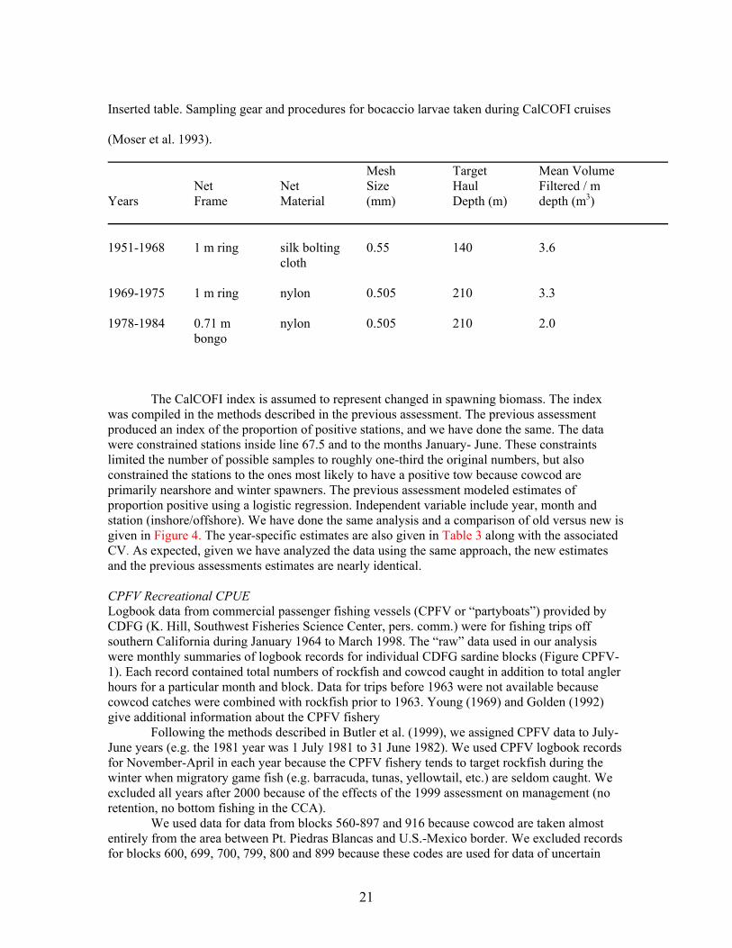
Inserted table. Sampling gear and procedures for bocaccio larvae taken during CalCOFI cruises

(Moser et al. 1993). Mesh Target Mean Volume Net Net Size Haul Filtered / m Years Frame Material (mm) Depth (m) depth (m3) 1951-1968 1 m ring silk bolting 0.55 140 3.6 cloth 1969-1975 1 m ring nylon 0.505 210 3.3 1978-1984 0.71 m nylon 0.505 210 2.0 bongo The CalCOFI index is assumed to represent changed in spawning biomass. The index was compiled in the methods described in the previous assessment. The previous assessment produced an index of the proportion of positive stations, and we have done the same. The data were constrained stations inside line 67.5 and to the months January- June. These constraints limited the number of possible samples to roughly one-third the original numbers, but also constrained the stations to the ones most likely to have a positive tow because cowcod are primarily nearshore and winter spawners. The previous assessment modeled estimates of proportion positive using a logistic regression. Independent variable include year, month and station (inshore/offshore). We have done the same analysis and a comparison of old versus new is given in Figure 4. The year-specific estimates are also given in Table 3 along with the associated CV. As expected, given we have analyzed the data using the same approach, the new estimates and the previous assessments estimates are nearly identical. CPFV Recreational CPUE Logbook data from commercial passenger fishing vessels (CPFV or “partyboats”) provided by CDFG (K. Hill, Southwest Fisheries Science Center, pers. comm.) were for fishing trips off southern California during January 1964 to March 1998. The “raw” data used in our analysis were monthly summaries of logbook records for individual CDFG sardine blocks (Figure CPFV-1). Each record contained total numbers of rockfish and cowcod caught in addition to total angler hours for a particular month and block. Data for trips before 1963 were not available because cowcod catches were combined with rockfish prior to 1963. Young (1969) and Golden (1992) give additional information about the CPFV fishery Following the methods described in Butler et al. (1999), we assigned CPFV data to July-June years (e.g. the 1981 year was 1 July 1981 to 31 June 1982). We used CPFV logbook records for November-April in each year because the CPFV fishery tends to target rockfish during the winter when migratory game fish (e.g. barracuda, tunas, yellowtail, etc.) are seldom caught. We excluded all years after 2000 because of the effects of the 1999 assessment on management (no retention, no bottom fishing in the CCA).

We used data for data from blocks 560-897 and 916 because cowcod are taken almost entirely from the area between Pt. Piedras Blancas and U.S.-Mexico border. We excluded records for blocks 600, 699, 700, 799, 800 and 899 because these codes are used for data of uncertain

22

origin. We excluded a few records that reported cowcod catches larger total rockfish catches and records with high catches from blocks with no cowcod habitat as likely errors.

To be consistent with the previous assessment, we assumed total angler hours reported on CPFV logs for blocks with rockfish catches during November-April was a measure of relative fishing effort for cowcod (see below). We used the logbook data to estimate catch rates measured as catch-per-unit-effort (CPUE, with adjustments described below) in units of numbers of fish per angler hour (fish hr-1).

Changes in angler’s gear likely had little effect on catch rates for cowcod because angler’s gear used on CPFV vessels has changed little since the early 1960’s. Anglers typically use one or two poles with 1-10 hooks per pole that are baited with live or dead bait.

Changes in the percent of fish that are identified to species and reported on logbooks as cowcod (rather than as rockfish) would also effect catch rates. We are not, however, aware of any changes in catch reporting until after the end our time series.

Changes in “effectiveness” of fishing effort may have changed catch rates for cowcod from CPFV logbook data. Catch rates tend to show optimistic trends if fishing effort has become more effective over time and pessimistic trends if fishing effort has become less effective over time. Aprior, we would expect that the advent of new technologies (gps etc.) would tend to favor more effective fishing effort .Butler et al. (1999), based upon knowledgeable sources, indicated that recreational fishing effort for rockfish may have moved from inshore areas to offshore areas during the 1960-1980’s and that initially, fishing effort during November-April in offshore areas was probably concentrated in relatively shallow areas around islands and bottom features.

Stratification for Modeling

Butler et al. (1999) stratified CPFV data spatially based on “pseudo-blocks” prior to fitting models and estimating trends in relative abundance. They found differences among blocks in CPUE trends because of differences among blocks in habitat quality. They designed a spatial stratification scheme based on CDFG sardine blocks that would accommodate differences in abundance trends among areas while reducing the number of strata (and model parameters) to a manageable number. We use the same area stratification.

Psuedo-Block 1=651 658 664 665 666 667 668 682 684 685 686 690 691 704 705 706 708 711 712 714 719 723 726 736 737 738 741 761 767 802 803 814 816 821 823 845 865 Psuedo-Block 2= 696 707 709 710 721 725 727 729 730 739 740 744 745 746 751 758 759 760 762 765 768 812 813 833 847 849 850 852 866 878 891 Psuedo-Block 3=827 829 678 683 815 897 678 866 724 728 742 743 747 748 749 750 763 764 766 769 770 806 807 808 809 820 825 826 834 835 836 840 846 853 854 855 856 861 863 864 867 868 871 872 882 883 889 890

The previous assessment used a General Additive Model to estimate CPUE from the California Commercial Passenger Fishing Vessel fleet. In this assessment, we have instead used a GLM approach to estimate CPUE. A logistic regression was used to estimate the proportion positive and a General Linear Model (gamma error assumption) was used to estimate the CPUE for only the positive tows. LSMEANS were calculated for the factor year. Separate estimates were produced for each pseudo-block incorporating month as an explanatory variable in the model. Similar to Butler et al. (1998,) we produced the SCB index by weighting the contribution to the overall index by the pseudo-blocks based upon the area inside each pseudo-block. Area in each block was based on the number of California reporting blocks that made up each pseudo-block. The estimates from the new CPUE series are very similar to that from the previous assessment (Figure 5 and Table 3). Only 3 new points were calculated and those are low relative to the series mean.

23

Outfall index of recruitment Both Los Angeles County and Orange County, Ca. sanitation departments routinely monitor the effects of outflow from their sewage treatment through the use of standardized trawls at fixed stations. Two other outfall data sets were considered (LA City and SD City). Consistent with the previous assessment, those series were not used because of a lack of cowcod catch and shorter time span. The trawls used by the sanitation departments are otter trawls with a 7.6 m headrope with a 1.25-1.3cm cod end mesh. Trawl speed was 1.5-2.5 knots and durations were ~10min. The outfall survey primarily catches very small/young (~ age 3) cowcod. The previous assessment used an arithmetic estimate of proportion positive as a measure of relative abundance of pre-recruit animals. We have analyzed the data in the same way. Our new series includes new data from 1998-2004 that was not included in the previous assessment as well as data 1970-1972 that was also not included. The 1970-1972 data are only from LA county, and is likely the reason those years were not included in the previous assessment. The index of recruitment is given in Figure 6 and Table 3. The values are identical in the overlapping years to those in Butler et al. (1999). The recruitment index is low throughout the 1980’s and 1990’s. There is evidence, however, of larger recruitment in recent years that will begin to contribute to the spawning biomass. Additional data not used in the previous assessment: (Data potentially used in the fully age-structured model. See Section 2) Length composition Length composition information from port sampled cowcod is relatively sparse. Cowcod have rarely been encountered in samples after the early 1980s. In order to provide the model with demographic information on the recreational catch, we produced year-specific length composition from a composite of 2 data sources. Recreational length information (1980-1989 and 1993-2002) was taken from the RecFIN website. These lengths were taken primarily as part of the MRFSS intercept sampling program used to estimate recreational catch. Additional recreational length observations (1975- 1979 and 1986-1989) were taken from a CPFV observer program in the SCB (per. Comm. Deb Wilson-Vandenberg CDF&G). Because cowcod are caught infrequently (sample size is generally small: see table 4) and all fish taken on a trip are usually sampled (in effect catch weighted), we assumed each length observation was random and representative of the recreational catch. The proportion at length from each year is given in Figure 8 and Table 5. Commercial length samples of cowcod are nearly non-existent. The only samples taken are from the late 1980’s, at the height of the set net fishery. Commercial fleet length information was taken from CalCOM (1986-1989 and 1995-1997). Port samplers collected individual lengths (FL) at unloading docks and the proportion at length data had been expanded based on catch by gear at the port and month level. The lengths were then converted (Love et al. 2001) to TL before binning. All lengths were binned in 2cm intervals from 10cm to 100cm TL. The commercial proportion at length is given in Figure 9 and Table 5. Although relatively few samples were taken, the commercial samples were much larger than the recreational samples (Figure 10). This is consistent with the knowledge that set net type gears, are likely to take large fish. Manned Submersible Visual Transect Survey. A single survey of the Cowcod Conservation Area (CCA) was completed using a manned submersible (Yoklavich et al. unpublished data). Transects were placed within a series of 1.5 x 1.5 km squares that were randomly chosen from a grid of squares overlying each bank. The results presented were from a 2002 sampling effort over eight rocky banks inside the CCA. Those banks were chosen because they were previously evaluated to be cowcod habitat (mixed sediment or rocky substrate at depths between 75 to 300 m). The survey platform was a two-person Delta

24

submersible capable of operating at depths up to 365 m and for speeds up to 1.5 knots. Safety considerations prevented the submersible from operating down steep slopes. A total of 95 dives were completed and the numbers of cowcod on all banks estimated using direct visual counts and one-sided line transect methods. Cowcod numbers were converted to biomass using recorded fish lengths and a length-weight relationship. The survey estimated 940 t (CV =25%) of cowcod in the study area within the CCA. The assessment team hosted an independent-internal panel (with outside reviewers from CIE and University) to review and advise the assessment team on the potential use of the new data in the assessment (see supplied materials on the review). Although advice from the review panel indicated that expanding the transect survey results to the entire SCB was not scientifically defensible, we estimated what fraction of the stock was not inside the CCA to develop a prior around the q. Preliminary expansion results indicate that the visual transect survey q=0.75 (essentially 1/3 of the stock lies outside the CCA- see Appendix IV and V). The estimate of q is uncertain because of potential biases in the survey method as well as expansion analysis. This expanded estimate may also serve as alternative assessment of cowcod abundance in 2002. Acoustic in combination with Remotely Operated Vehicle (ROV) Survey Another version of a fishery independent survey aimed at rockfish like cowcod is presently being developed. This survey involves the use of acoustic sampling methods and a remotely operated vehicle (ROV) to monitor size and species composition. The ROV may also be used to estimate density in areas the acoustic signal is uninformative due to bottom echo. The survey has been conducted since 2004, but has not yet developed formal protocols and has not been peer reviewed (pers. Comm. John Butler). Thus this survey is not used in this assessment. It may be a source of information for future assessments. Cowcod Intensive Sampling Because of the low stock abundance and the low encounter rate of cowcod in the CalCOFI survey, a more intensive ichthyoplankton survey was developed. This survey is designed to monitor decadal changes in spawning biomass. The survey sampled more intensely in a limited geographical area to monitor rebuilding inside the CCA using the same methods as the CalCOFI survey. The intensive sampling began in 2000, but only two years of samples have been identified to species. Because of the limited temporal series and lack of a formal review of the survey methods it is not used in this assessment. However it may be a source of decadal changes in future assessments. Hook and Line Survey The NWFSC began conducting a hook and line survey of rockfish in the SCB. The survey initially began in 2003 and was continued in 2004. Several cowcod have been recorded in this survey, but due to the limited time scale, lack of formal survey protocols and the lack of peer review, it has not been included in this assessment. It may be a source of information in future assessments. RecFIN recreational Fishery CPUE We considered creating a separate index of recreational CPUE for private boats and party boats using the RecFIN port intercept data and the Steven and MacCall (2004) approach. The party boat index is drawn from the same sampling universe as the CPFV logbook index. Because of the overlap with the logbook data and few samples, the RecFIN index was not used in the modeling. The RecFIN private boat index was based on very sparse sampling and was unusually noisy, therefore it was not considered a realistic assessment of population abundance changes. Both indices were produced using a standard a delta glm approach with season as an explanatory variable. The RecFIN based indices are given in Figure 7 and Table 3.

25

(The next section presents our analysis of the population using a fully age structure model.)

SECTION 2: Assessment Model

Previous Assessment

The previous assessment was conducted in 1998 using a delay-difference model (Butler et al. 1999). In that previous assessment, the stock boundary was identical to the boundary used in this assessment. The analytical team chose the delay difference model because they believed there was not enough length/age information to do a more complex analysis. They assumed that the fishable biomass was comprised of fish > 40 cm FL, because that size also corresponded to the approximate size at maturity (fishable biomass= spawning biomass). The assessment assumed the fishable biomass was proportional to the CPFV recreational CPUE and the CalCOFI larval survey. The assessment assumed that recruitment was proportional to the Outfall index lagged by seven years and controlled by a random walk process. The previous assessment concluded that the fishable biomass was under 250 t and ~7% of unfished in 1998. For more specific information on the previous assessment and for our update of that assessment see appendix 1.

Current Assessment approach

In this section we explore the use of an age-structured analysis. Structural changes to the assessment include the assumption of a Beverton Holt spawner-recruit function (S/R) and that we model numbers at age. The assumption of an underlying S/R relationship is a traditional fishery assumption and its shape will be critical to rebuilding analysis. We address 2 important questions with this model. What is the ending biomass and associated depletion level (ending biomass/ virgin biomass)? What is the expected productivity of the stock as assumed by the BH S/R steepness parameter (h)?

Star Panel Data Considerations The STAR panel considered all the data sources and in discussion with the STAT team decided that only the CPFV CPUE series and the Visual transect estimate were justified for use in the current assessment. Both the Outfall and CalCOFI indices were series with too few positive tows, and the abundance of the zero catch years were problematic for the lognormal error assumption. Likewise, the proportion at length information was not used because of its general noisy nature and that the assessment model had difficulty in fitting to the data. Both STAR panel and STAT team agreed that the visual survey should be treated as a measure relative abundance with prior information about q (see Appendix IV and V). Model Components. The following models use the likelihood components listed below: Fishery catch 1916-2005 (recreational and commercial) CPFV recreational fishery CPUE 1963-2000 Visual Transect Survey estimate of biomass (2002) This following data were not part of the Butler et al. (1999) assessment: Fishery catch 1999-2005 CPFV recreational CPUE years (1998-2000)

26

Visual transect survey estimate (2002) The following assumptions apply to the base case model described below: The population can be described by a single sex life history. Catch is known without error. Natural mortality is assumed =0.055 Recruitment process is described by a Beverton-Holt Stock-Recruit relationship. Selectivity patterns of the fishery and CPUE series were assumed. Selectivity for the fishery, CPFV and CPUE are length based. The CV of the length-at-age relationship is assumed =0.05. A diffuse normal prior (sd=1000) is assumed for each estimated parameter (except visual transect survey q). All models begin in 1916 with the population in equilibrium assuming a total catch of 2 t. The base cases and sensitivity analysis were performed in SS2 Version 1.19. Complete data and control files are given in Appendix III. Base Case . Simple stock reduction Base case 1 is a stock reduction model that is essentially an age-structured production model, where lnR0 (initial recruitment) is the carrying capacity and h is analogous to the intrinsic rate of increase. The model assumes a single fishery (combined recreational and commercial). A total of 4 parameters are estimated ( lnR0, initial F of the combined recreational/commercial fishery, and 2 survey q parameters). This model is conceptually close to the delay difference of the previous assessment. The model uses CPFV CPUE, and visual transect survey information. Length information is not used. Selectivity patterns of the single fishery and the CPFV CPUE series is assumed to be the same as the female maturity ogive. In other words, the vulnerable biomass is the mature biomass. This assumption is essentially the same assumption used by Butler et al. (1999), where they modeled knife edge recruitment into the fishery at 40 cm (FL). The visual transect survey is treated as a relative index with some information about its catchability (q) because the survey was designed to be an absolute estimate; a normal prior around q=0.75 and a CV=0.5. This prior comes from a recommendation of error bounds by the independent survey review panel and considerations of the STAR Panel. The prior is however, subjective. The CV associated with the visual survey estimate is assumed to be the reported 0.25. Selectivity of the visual survey is 1 for all ages, because the visual survey method assumed that all fish are seen along the transect line. Recruitment is constrained to a BH S/R curve with h fixed at 3 levels (h=0.4, 0.5 and 0.6) and lnR0 estimated. The inputted CV associated with each survey time series (except the visual transect survey) was iteratively adjusted by a multiplicative scaling factor to achieve internal model consistency. Base Case Model Results Models using all 3 levels of h depict similar pictures of a population that declined to very low levels during the 1990’s and remains below the overfished threshold in 2005 (14-21% of unfished spawning biomass). All models indicate that the population reached very low stock sizes in the 1990’s and has since increased. Spawning stock biomass in 2005 was estimated to be 444-642 (t), for h=0.4-0.6, respectively. The likelihoods of all individual components, parameter estimates and values of important fixed parameters from all three models are given in Table 6. Figure 11 depicts observed and predicted values for each survey from h=0.4. Figure 12 depicts observed and predicted values for each survey from h=0.5. Figure 13 depicts observed and predicted values for each survey from h=0.6. Figure 14 depicts the assumed selectivity pattern (same as female maturity ogive).

27

Table 7 depicts the estimated time series of spawning biomass, recruitment and harvest rates from all 3 levels of h. Estimates of the population numbers at age for the most likely model are given in Appendix VI. Uncertainty and Sensitivity For each of the three potential base case models, we performed sensitivity analysis to determine the effects of data, and assumptions on model performance. We performed sensitivity analysis to the assumed levels of M and h. We also examined the effects of changing the visual survey q and associated CV. The results are presented in Table 8. In the original document (prior to STAR Panel), we examined the effects of doubling and halving pre-1970 catch on a similar model. Although not presented in this post-STAR panel document, the changes in historical catch did not drastically alter our perception of stock status. At the STAR panel meeting, we also estimated a power coefficient relating the CPFV CPUE series q and the population abundance. Estimating this power coefficient improved the fit to the CPFV CPUE series and indicated that the series may show hyperdepletion (coefficient =1+0.6). However, there was no biological/fishery justification for estimation of this parameter at this time. It may be useful to investigate this phenomenon in subsequent assessments. We also did a sensitivity analysis that removed all priors and the model estimates were not greatly different as the prior on visual survey q was the only informative prior and it was only somewhat informative. Harvest Projections and Decision Tables Forecasted yields using the F50%SPR proxy for MSY (both 40-10 adjusted and not adjusted) were calculated. The harvest projections using an F50%SPR rate for the years 2006-1017 are given in Table 9. A decision table was constructed that evaluates the effects of choosing an OY catch from any one of the levels of assumed h to base management action if one of the other base cases is actually a better population representation The decision table is given in Table 10. Because cowcod are overfished the quotas will be set by a separate rebuilding analysis and not based upon the forecasts in this document. Forecasts and decision tables in this document are for entertainment purposes only. Rebuilding parameters and Reference Points In the PFMC groundfish group, a stock is considered overfished if the current spawning biomass is less than 25% of the unfished biomass. At the current abundance, the cowcod population remains overfished. Overfishing (different from being overfished) occurs if the actual harvest rate exceeds the harvest rate at MSY or its proxy (F50%SPR). With almost no catch occurring since 2001, overfishing is not presently occurring. Reference Parameters and quantities needed for rebuilding are given in Table 11. A separate rebuilding analysis has not yet been completed. General Comments about all models All models indicate that cowcod in the SCB are still below the overfished threshold (spawning biomass <25% of unfished). All models indicate that the population has been stable to increasing over the last 10 years. This is not surprising because catch has dropped to near zero, and the data sources that extended beyond 2000 have generally been more positive. Over the range of models explored, the ratio of 2005 spawning biomass/virgin spawning biomass ranged from 14-21%. No matter the model configuration, it is clear that management action was necessary to protect the stock in 1999. Although the level of h was assumed in each model run, the STAR panel recommend that h=0.5 be considered the base model configuration with the highest probability of being true (40% probability) and that h=0.4 and h=0.5 are less likely (30%).

28

The overall view of the population status is not greatly affected by estimates of historical catch. Previous STAR panels have acknowledged that historical catch is uncertain and that its effects on population trends should be considered. Information on catch prior to the mid 1970’s is not generally available. Butler et al. (1999) made good use of available information to determine estimates of historical catch going back more than 50 years, and the estimates have subsequently been accepted by both review panels and journal review. However, those estimates are still very uncertain. It is likely that errors of omission of catch are greater than addition, but the sensitivity analysis indicates that even doubling pre 1970 catch does not greatly affect estimates of terminal spawning biomass or depletion. Other assessment issues are probably a larger source of uncertainty. Another question that needs to be asked is if the assumed curvature of the BH S/R relationship (h) is reasonable? Estimates of h from more data rich rockfish assessments include canary rockfish h=0.29 (Methot and Piner 2002) and yelloweye rockfish h=0.4 (Methot et al. 2003). Both are large rockfish species that showed a similar magnitude of decline as cowcod. However those estimates of h are much smaller than the meta-analysis estimate from Dorn (2002). We do not know if the assumed levels of h (0.4-0.6) are appropriate, but they are likely a reasonable range to base management action until we understand productivity of this species better. The outside assessment of cowcod abundance from the Visual Transect survey by Yoklavich et al. (unpublished data), presents the most optimistic picture of the cowcod population. Their independent assessment methodology indicates that the cowcod population in the CCA was roughly twice the 2002 biomass estimated by this stock assessment. We do not know if direct observation using transect theory is more realistic than the traditional stock assessment method presented in this document. It does appear to support the larger estimates of biomass from this assessment relative to the Delay Difference modeling used previously. Despite the support for higher biomass from the visual survey, there appears a general mis-match between the population dynamics implied by the CPFV cpue series and the visual transect estimate. The more fitting power (less freedom in the visual q parameter) given to the visual transect estimate, the poorer the fit to the CPUE series. If the transect survey is an unbiased and reasonably precise estimate of abundance, then the assessment results presented here are likely too pessimistic. We also do not fit the CPFV CPUE series well, with the population abundance underestimating the cpue decline. If the CPFV CPUE series is an accurate depiction of population change, this assessment is likely too optimistic. At this time, we do not know with certainty which picture is correct. Conclusions The analytical team asked itself if any of the models presented in this document are realistic? The answer is probably no. All the data sources used have their problems and are likely biased, although we do not know the magnitude or direction of that bias. It is not clear if recreational CPUE is truly proportional to biomass, especially with the likely undocumented changes the fleet has made and the improvements the industry has made in technology. It is hard to believe that over the 40 years the series spans, the fishing power, reporting rates and targeting practices have not changed. Finally, the visual survey has its own questions regarding sampling and the magnitude/direction of the associated error, and that availability of only a single estimate makes evaluating its reliability as an absolute estimate difficult. Even if the transect estimate is an unbiased and relatively precise measure of stock abundance, we are not sure that pinning the model to the estimate when it may be somewhat conflicting with other series is the best solution to produce management advice. However, it is clear that alternative (to trawl based methods) methods of surveying, such as transect surveys, are necessary to monitor cowcod populations. This is an area of research that will be needed to adequately address cowcod management.

29

The results of this assessment corroborate the 1999 assessment in that cowcod are very likely at a small fraction of their hypothetical unfished state and below the overfished threshold. Although the stock status in this assessment is more optimistic than in the previous assessment, this is due in part to the different assumptions in this assessment. Estimates of harvest rates near MSY are similar to those described by Jacobsen et al. (2001) using surplus production models (schaefer and ASPIC). Catch levels seen throughout the 1980s are clearly too high and it is may be that the Pacific Fishery Management Council default harvest rate of F50%SPR is too aggressive for this species. However, the available information indicates that the population may have stabilized and that it is increasing in the most recent years. Given that reported catch has been near zero for close to a decade, this is not unexpected. If the population does not increase with the level of catches assumed in the model, then it is likely no reasonable management strategy will be successful. Most troubling to the assessment team is what future assessment will do. It is not clear that any of the new survey methods discussed in the data section will be both useful (quantitative, synoptic coverage etc.) and repeated in the near future. Very little new data was available for this assessment beyond what was available for the 1999 assessment, and the future of survey information is not certain. Survey type information will be most useful if it is done consistently and often. A more directed and consistent measure of abundance that can be done at least biannually is sorely needed. Research Needs

1. Consistent and synoptic monitoring of relative/absolute biomass. This new survey should cover areas both inside and outside the CCA.

2. Work on defining stock boundary. The choice of stock boundary in the assessment was based on historical definitions, but may not be accurate. Does Mexico or the Monterey INPFC area harbor a portion (substantial?) of the stock.

3. Determine if fish move in response to environmental signals. There is some indication that fish may have moved from the assessed area during regime type environmental changes.

4. Collection and analysis of biological data. Better define growth, mortality and maturity. 5. As habitat classification maps are developed for the SCB, these will likely be useful to

construct the CPUE and Survey time series. 6. Establish different criteria (reference points, rebuilding strategies) for truly data poor

species that do not have the quality or quantity of data needed to estimate the current suite of assessment/management quantities. It is unknown if trying to provide the detailed advice currently requested by the PFMC may contribute to erroneous advice relative to maybe much simpler assessment advice (ie. Abundance is increasing/decreasing).

Acknowledgements The stat team is grateful to many people for their help, including the STAR Panel, C. Show, C. Reiss, J. Wallace, J. Butler, R. Conser, M. Yoklavich, M. Love, K. Forney and many others too numerous to be named. The biological staff at the Orange County, LA County, LA City and San Diego County Sanitation departments were more than helpful during our constants data requests. We would also like to thank Buckner, for knowing how to fetch. LITERATURE CITED Ahlstrom, E. H. 1959. Vertical distribution of pelagic fish eggs and larvae off California and Baja California. Fish. Bull. U.S. 60:107-146.

30

Ally, J.R., D.S. Ono, R.B. Read and M.Wallace. 1991. Status of major southern California marine sport fish species with management recommendations, based on analyses of catch and size composition data collected on board commercial passenger fishing vessels from 1985 through 1987. Calif. Dept. Fish and Game, MRD Admin. Rep. No. 90-2. 375p. Barnes, J.T., M. Yaremko, L. Jacobson, N.C.H. Lo and J. Stehly. 1997. Status of the Pacific sardine (Sardinops sagax) resource in 1996. NOAA Tech. Mem. NOAA-TM-NMFS-SWFSC-237. 40p. Beamish, R. J. and D. A. Fornier. 1981. A method for comparing the precision of a set of age determinations. Can. J. Fish. Aquat. Sci. 38: 982-983. Beauchamp, J., and J. Olson. 1973. Corrections for bias in regression estimates after logarithmic transformation. Ecology 54: 1403-1407. Boehlert, G. W. and M. M. Yoklavich. 1984. Reproduction, embryonic energetics, and the maternal-fetal relationship in viviparous genus Sebastes (Pisces: Scorpaenidae). Biol. Bull. 167: 354-370. Brinton, E. and A. W. Townsend. 1981. A comparison of euphausiid abundances from bongo and 1-m CalCOFI nets. Calif. Coop. Oceanic Fish. Invest. Repts. 22:111-125. Brodziak, J., L.D. Jacobson, R. Lauth, and M. Wilkins. 1997. Assessment of the Dover sole stock for 1997. In: Pacific Fishery Management Council. 1997. Appendix: Status of the Pacific Coast Groundfish Fishery through 1997 and recommended biological catches for 1998: Stock assessment and fishery evaluation. Pacific Fishery Management Council, 2130 SW Fifth Avenue, Suite 224, Portland, Oregon, 97201. Butler, J. L., L. D. Jacobson and J.T. Barnes. 1998. Stock assessment of blackgill rockfish. In: Pacific Fishery Management Council. 1998. Appendix: Status of the Pacific Coast Groundfish Fishery through 1998 and recommended biological catches for 1999: Stock assessment and fishery evaluation. Pacific Fishery Management Council, 2130 SW Fifth Avenue, Suite 224, Portland, Oregon, 97201. Butler, J. L., L. D. Jacobson and J.T. Barnes. 1999. Stock assessment of cowcod rockfish. In: Pacific Fishery Management Council. 1999. Appendix: Status of the Pacific Coast Groundfish Fishery through 1999 and recommended biological catches for 2000: Stock assessment and fishery evaluation. Pacific Fishery Management Council, 2130 SW Fifth Avenue, Suite 224, Portland, Oregon, 97201. Chang, W. Y. B. 1982. A statistical method of evaluating the reproducibility of age determination. Can. J. Fish. Aquat. Sci. 39: 1208-1210. Collins, R.A. and S.J. Crooke. MS. An evaluation of the commercial passenger fishing vessel record system and the results of sampling the southern California catch for species and size composition, 1975-1978. 147p.

31

Deriso, R.B., J.T. Barnes, L.D. Jacobson and P.J. Arenas. 1996. Catch-at-age analysis for Pacific sardine (Sardinops sagax), 1983-1995. Calif. Coop. Oceanic Fish. Invest. Rep. 37:175-187. Dorn, M.W. 2002. Advice on west coast rockfish harvest rates from Bayesian meta-analysis of stock recruitment relationships. N. Amer. J. Fish. Mngt. 22: 280-300. Eigenmann, C. H. and C. H. Beeson. 1894. A revision of the fishes of the subfamily Sebastinae of the Pacific Coast. Proc. U. S. Nat. Mus. 17: 375–407. Eschmeyer, W. N., E. S. Herald, and H. Hammann. 1983. A field guide to Pacific Coast fishes of North America: from the Gulf of Alaska to Baja, California. Houghton Mifflin, Boston. Fornier D. and C. P. Archibald. 1982. A general theory for analyzing catch at age data. Can. J. Fish. Aquat. Sci. 39: 1195-1207. Golden, M.F. 1992. Marine recreational fisheries, p. 204–207. In: W.S. Leet, C.M. Dewees, and C.W. Haugen. California’s living marine resources and their utilization. Calif. Sea Grant Ext. Publ. UCSGEP-92-14. Heincke, F. 1913. Investigations on the plaice. General report. 1. Plaice fishery and protective regulations. Part I. Rapp. P.-V. Reun. Cons. Perm. Int. Explor. Mer 17A: 1–153. Heinmann, R.F. G. 1968. California Marine Fish Catch for 1968. Sacramento Ca. 1970. Cal. Dept Fish. Game Bulletin. Hewitt, R. P. 1988. Historical review of the oceanographic approach to fishery research. Calif. Coop. Oceanic Fish. Invest. Repts. 22:111-125. Hill, K.T., and J.T. Barnes. 1998. Historical catch data from California’s commercial passenger fishing vessel fleet: status and comparisons of two sources. Calif. Dept. Fish and Game, Marine Region Tech. Rep. No. 60. Hill, K. T., M. Yaremko, and L. D. Jacobson. 1999. Status of the Pacific mackerel resource and fishery in 1998. Calif. Dep. Fish Game. Marine Region Admin. Rep. 99-3. 57 p. Hoenig, J. M. 1983. Empirical use of longevity data to estimate mortality rates. Fish. Bull. 82: 898-903. Jacobson, L.D., N.C.H. Lo and J.T. Barnes. 1994. A biomass based assessment model for northern anchovy, Engraulis mordax. Fish. Bull., U.S. 92:711-724. Jacobson, L.D., S. Ralston, and A.D. MacCAll. 1996. Historical larval abundance indices for bocaccio rockfish (Sebastes paucispinis) from CalCOFI data. National Marine Fisheries Service, Southwest Fisheries Science Center, Administrative Report LJ-96-06. Jacobson, L. D., S. X. Cadrin, and J. R. Weinberg. 2001. Tools for estimating surplus production and Fmsy in any stock assessment model. North American Journal of Fisheries Management. Vol 22 (1): pp. 326-338. Jensen, A. L. 1997. Origin of the relation between K and Linf and synthesis of relations among life history parameters. Can. J. Fish. Aquat. Sci. 54: 987-989.

32

Johnson, K. A. 1997. Rockfish (Sebastes spp.) recruitment to soft bottom habitats in Monterey Bay, CA. M. S. Thesis. Moss Landing Marine Laboratories, California State University, Stanislaus. Karpov, K.A., D.P.Albin and W.H. Van Buskirk. 1995. The marine recreational fishery in northern and central California; A historical comparison (1958-86), a status of the stocks (1980-86), and effects of changes in the California current. Calif. Dept. Fish and Game Fish Bull.(176): 192p. Kimura, D. K. 1985. Changes to stock reduction analysis indicated by Schnute's general theory. Can. J. Fish. Aquat. Sci. 42: 2059-2060. Kimura, D. K, J. W. Balsiger, and D. H. Ito. 1984. Generalized stock reduction analyses. Can. J. Fish. Aquat. Sci. 41: 1325-1333. Kimura, D. K., and J. V. Tagart. 1982. Stock reduction analysis, another solution to the catch equations. Can. J. Fish. Aquat. Sci. 39: 1467-1472. Love, M. S., J. E. Caselle, and W. V. Buskirk. 1998. A severe decline in the commercial passenger fishing vessel rockfish (Sebastes spp.) catch in the Southern California Bight, 1980–1996. CalCOFI Rep. 39: 180–195. Love, M. S., P. Morris, M. McCrae and R. Collins. 1990. Life History aspects of 19 rockfish species (Scorpaenidae: Sebastes) from the Southern California Bight. NOAA Tech. Rep. NMFS 87 38 pp. Love, M.S., M.Yoklavich, and L. Thorsteinson. 2002. The Rockfishes of the northeast Pacific. University of Cal. Press. Berkely Ca. 405p. Mangel, M. and P. E. Smith. 1990. Presence-absence sampling for fisheries management. Can. J. Fish. Aquat. Sci. 47: 1875-1887. MacCall, A.D., G.D. Stauffer and J-P. Troadec. 1975. Report on CF&G – NMFS cooperative stock assessment, fishery evaluation, and fishery management of southern California recreational and commercial fisheries. NMFS, SWFC Admin. Rpt. LJ-74-24. 144p. MacCullagh, P., and J.A. Nelder. 1983. Generalized linear models. Chapman and Hall, New York. Mearns, A. J. 1979. Abundance, composition and recruitment of nearshore fish assemblages on the Southern California mainland shelf. Calif. Coop. Oceanic Fish. Invest. Repts. 20:111–119. Methot, R.D. 1989. Synthesis model: an adaptable framework for analysis of diverse stock assessment data. Int. N. Pac. Fish. Comm. Bull. 50: 259-277. Methot R.D., and K.R. Piner. 2002. Status of Canary Rockfish Resource off California, Oregon and Washington in 2001. In: Pacific Fishery Management Council. 20902. Appendix: Status of the Pacific Coast Groundfish Fishery through 2002 and recommended biological catches for

33

2003: Stock assessment and fishery evaluation. Pacific Fishery Management Council, 2130 SW Fifth Avenue, Suite 224, Portland, Oregon, 97201. Methot R.D., F., Wallace, and K.R. Piner. 2003. Status of Yelloweye Rockfish off the West Coast of the United States in 2002. In: Pacific Fishery Management Council. Appendix: Status of the Pacific Coast Groundfish Fishery through 2003 and recommended biological catches for 2004: Stock assessment and fishery evaluation. Pacific Fishery Management Council, 2130 SW Fifth Avenue, Suite 224, Portland, Oregon, 97201 Miller, D.J., and D. Gotshall. 1965. Ocean sportfish catch and effort from Oregon to Point Arguello, California. Calif. Dept. Fish and Game Fish Bull. (130): 135p. Miller, D, J. and R. N. Lea. 1972. Guide to the Coastal Marine Fishes of California. Calif. Dept. Fish and Game. Fish Bull. 157: 1-235. Moser, H. G. 1967. Reproduction and development of Sebastodes paucispinis and comparison with other rockfishes off Southern California. Copeia 1967:773– 797. Moser, H. G. 1996. Scorpaenidae. In The Early Stages of the Fishes of the California Current Region. CalCOFI Atlas No. 33. H. G. Moser, Ed. Moser, H. G., E. H. Ahlstrom, and E. M. Sandknop. 1977. Guide to the identification of scorpionfish larvae (family Scorpaenidae) in the eastern Pacific with comparative notes on species of Sebastes and Helicolenus from other oceans. U.S. Dep. Commer., NOAA Tech. Rep. NMFS Circ. 402. 71 pp. Moser, H. G. and G. W. Boehlert. 1991. Ecology of pelagic larvae and juveniles of the genus Sebastes. Env. Biol. Fish. 30:203–224. Moser, H. G., R. L. Charter, P. E. Smith, D. A. Ambrose, S. R. Charter, C. A. Meyer, E. M. Sandknop, and W. Watson. 1993. Distributional atlas of fish larvae and eggs in the California Current region: taxa with 1000 or more total larvae, 1951 through 1984. CalCOFI Atlas 31. 233 pp. Moser, H. G., R. L. Charter, P. E. Smith, D. A. Ambrose, S. R. Charter, C. A. Meyer, E. M. Sandknop, and W. Watson. 1994. Distributional atlas of fish larvae and eggs in the California Current region: taxa with less than 1000 total larvae, 1951 through 1984. CalCOFI Atlas 32. 181 pp. Ohman, M. D and P. E. Smith. 1995. A comparison of zooplankton sampling methods in the CalCOFI time series. Calif. Coop. Oceanic Fish. Invest. Repts. 36:153–158. Ralston, S., J. N. Ianelli, R. A. Miller, D. E. Pearson, D. Thomas, and M. E. Wilkins. 1996. Status of bocaccio in the Conception/Monterey/Eureka INPFC areas in 1996 and recommendations for management in 1997.

34

Ricker, W. E. 1975. Computation and interpretation of biological statistics of fish populations. Bull. Fish. Res. Bd. Can. No. 191. 382p. Robson, D. S. and D. G. Chapman. 1961. Catch curves and mortality rates. Trans. Am. Fish. Soc. 90: 181–189. Rogers, J. B., M. Wilkins, D. Kamakawa, F. Wallace, T. Builder, M. Zimmerman, M. Kander, and B. Culver. 1996. Status of the remaining rockfish in the Sebastes complex in 1996 and recommendation for management in 1997. Appendix II to the Status of the Pacific Coast Groundfish Fishery Through 1996 and Recommended Acceptable Biological Catches for 1997. Schnute, J. 1985. A general theory for analysis of catch and effort data. Can. J. Fish. Aquat. Sci. 42: 414-429. Sims, S.E. 1982. Algorithms for solving the catch equation forward and backward in time. Can. J. Fish. Aquat. Sci. 39: 197-202. Stevens, E. G., R. L. Charter, H. G. Moser, and C. A. Meyer. 1990. Ichthyoplankton and station data for California Cooperative Oceanic Fisheries Investigations survey cruises in 1984. U.S. Dep. Commer., NOAA Tech. Memo., NOAA-TM-NMFS-SWFSC-141. 157 pp. Stull, J. K. 1995. Two decades of marine biological monitoring, Palos Verdes, California, 1972 to 1992. Bull. Southern California Acad. Sci. 94(1). pp. 21– 45. Stull, J. K. and C.L. Tang. 1996. Demersal fish trawls off Palos Verdes, Southern California, 1973–1993. CalCOFI Rep., Vol. 37. pp 211–240. Wine, V. and T. Hoban. 1976. Southern California independent sportfish sampling survey annual report – July 1, 1975 – June 30, 1976. Calif. Dept. Fish and Game, MRD Admin. Rep. No. 76-14. 299p. Young, P.H. 1969. The California partyboat fishery 1947–1967. Calif. Dept. Fish and Game, Fish Bull. 145. 91p..

35

Table 1. The landings of cowcod in the Southern California Bight by year and fishery. Units are metric tones rounded to the nearest tenth.

year commercial recreational TOTAL year commercial recreational TOTAL 1916.0 8.8 8.8 1960.0 30.0 36.0 66.1 1917.0 14.1 14.1 1961.0 24.0 33.0 56.5 1918.0 14.9 14.9 1962.0 21.0 35.0 56.0 1919.0 9.7 9.7 1963.0 26.0 30.0 55.9 1920.0 10.2 10.2 1964.0 18.0 34.0 51.6 1921.0 8.6 8.6 1965.0 20.0 43.0 63.0 1922.0 7.8 7.8 1966.0 22.0 85.0 107.0 1923.0 9.2 9.2 1967.0 21.0 110.0 130.8 1924.0 8.6 8.6 1968.0 21.0 77.0 97.7 1925.0 9.9 9.9 1969.0 20.0 53.0 72.8 1926.0 13.6 13.6 1970.0 23.0 79.0 102.2 1927.0 11.6 11.6 1971.0 24.0 62.0 86.0 1928.0 11.6 11.6 1972.0 36.0 90.0 125.8 1929.0 10.9 10.9 1973.0 48.0 97.0 145.4 1930.0 13.1 13.1 1974.0 47.0 129.0 175.9 1931.0 13.2 13.2 1975.0 51.0 109.0 160.5 1932.0 10.2 10.2 1976.0 53.0 140.0 193.9 1933.0 8.7 8.7 1977.0 45.0 100.0 144.9 1934.0 8.3 8.3 1978.0 45.0 73.0 117.6 1935.0 8.7 8.7 1979.0 62.0 86.0 147.7 1936.0 8.3 8.3 1980.0 50.2 96.4 147.0 1937.0 7.8 7.8 1981.0 64.6 26.6 91.0 1938.0 6.6 6.6 1982.0 47.4 97.0 144.0 1939.0 6.0 6.0 1983.0 69.1 15.1 84.0 1940.0 6.5 6.5 1984.0 151.1 21.2 172.0 1941.0 6.2 6.2 1985.0 152.4 36.0 188.0 1942.0 2.6 2.6 1986.0 147.3 46.0 193.0 1943.0 5.0 5.0 1987.0 76.8 29.1 106.0 1944.0 11.6 11.6 1988.0 86.8 13.9 101.0 1945.0 24.0 24.0 1989.0 17.4 20.6 38.0 1946.0 20.2 20.2 1990.0 10.4 21.6 32.0 1947.0 16.7 16.7 1991.0 7.1 20.9 28.0 1948.0 15.3 15.3 1992.0 17.3 20.7 38.0 1949.0 16.5 16.5 1993.0 14.9 9.7 24.0 1950.0 21.1 21.1 1994.0 13.7 26.0 39.0 1951.0 24.0 9.0 24.5 1995.0 23.3 1.7 25.0 1952.0 23.0 10.0 32.5 1996.0 24.6 5.4 30.0 1953.0 20.0 13.0 33.6 1997.0 7.3 1.8 9.0 1954.0 27.0 24.0 50.3 1998.0 1.2 2.8 4.0 1955.0 27.0 42.0 69.0 1999.0 3.5 3.8 7.0 1956.0 28.0 49.0 76.4 2000.0 0.4 4.5 5.0 1957.0 32.0 37.0 69.4 2001.0 0.5 1958.0 35.0 33.0 68.1 2002.0 0.5 1959.0 39.0 22.0 61.2 2003.0 0.5

2004.0 0.5 2005.0 0.5

36

Table 2. The number of stations and the number of positive stations (collected at least 1 cowcod) for each survey and CPUE index used in assessment.

CalCOFI CPFV Outfall RecFIN party boat RecFIN private

year # obs #

positive # obs #

positive # obs #

positive #

obs #

positive #

obs #

positive 1950 94 6 n/a n/a n/a n/a n/a n/a n/a n/a 1951 137 3 n/a n/a n/a n/a n/a n/a n/a n/a 1952 177 4 n/a n/a n/a n/a n/a n/a n/a n/a 1953 181 10 n/a n/a n/a n/a n/a n/a n/a n/a 1954 142 4 n/a n/a n/a n/a n/a n/a n/a n/a 1955 156 2 n/a n/a n/a n/a n/a n/a n/a n/a 1956 142 3 n/a n/a n/a n/a n/a n/a n/a n/a 1957 171 8 n/a n/a n/a n/a n/a n/a n/a n/a 1958 187 3 n/a n/a n/a n/a n/a n/a n/a n/a 1959 195 9 n/a n/a n/a n/a n/a n/a n/a n/a 1960 73 3 n/a n/a n/a n/a n/a n/a n/a n/a 1961 64 4 n/a n/a n/a n/a n/a n/a n/a n/a 1962 77 0 n/a n/a n/a n/a n/a n/a n/a n/a 1963 109 3 141 31 n/a n/a n/a n/a n/a n/a 1964 112 3 252 53 n/a n/a n/a n/a n/a n/a 1965 169 6 273 73 n/a n/a n/a n/a n/a n/a 1966 23 1 317 86 n/a n/a n/a n/a n/a n/a 1967 71 4 308 76 n/a n/a n/a n/a n/a n/a 1968 144 17 279 73 n/a n/a n/a n/a n/a n/a 1969 116 9 329 70 n/a n/a n/a n/a n/a n/a 1970 n/a n/a 327 58 32 4 n/a n/a n/a n/a 1971 n/a n/a 333 84 31 6 n/a n/a n/a n/a 1972 197 6 349 96 32 9 n/a n/a n/a n/a 1973 n/a n/a 351 170 60 18 n/a n/a n/a n/a 1974 n/a n/a 340 157 57 5 n/a n/a n/a n/a 1975 215 0 358 205 59 16 n/a n/a n/a n/a 1976 n/a n/a 369 151 55 2 n/a n/a n/a n/a 1977 n/a n/a 365 114 66 6 n/a n/a n/a n/a 1978 171 0 126 47 56 1 n/a n/a n/a n/a 1979 n/a n/a 301 98 79 4 n/a n/a n/a n/a 1980 n/a n/a 450 178 81 4 700 12 319 8 1981 141 0 442 179 80 2 630 24 171 2 1982 n/a n/a 387 107 81 1 470 13 269 7 1983 n/a n/a 399 133 80 1 539 19 n/a n/a 1984 67 0 431 123 82 2 675 19 n/a n/a 1985 68 0 364 70 66 0 668 18 183 2 1986 70 0 347 69 82 5 646 9 113 2 1987 72 0 419 58 80 1 n/a n/a 74 4 1988 72 0 408 70 80 3 240 2 240 2 1989 67 1 418 75 80 0 n/a n/a n/a n/a 1990 68 1 409 78 80 1 n/a n/a n/a n/a 1991 67 1 426 100 94 0 n/a n/a n/a n/a 1992 72 0 376 57 106 0 n/a n/a n/a n/a 1993 71 0 374 36 112 1 138 4 140 5 1994 69 0 378 43 100 2 218 8 131 7 1995 69 0 409 43 95 0 n/a n/a n/a n/a 1996 68 0 445 54 80 1 n/a n/a 112 4 1997 70 0 419 17 82 0 n/a n/a 41 3 1998 71 1 465 43 82 0 327 2 66 4 1999 81 3 386 12 99 3 949 10 191 3 2000 70 2 150 5 83 9 528 4 n/a n/a 2001 70 0 n/a n/a 84 5 n/a n/a n/a n/a 2002 71 5 n/a n/a 91 3 n/a n/a n/a n/a

37

Table 3 . The survey and CPUE estimates used in the assessment of cowcod. CalCOFI CPFV Outfall RecFIN Party boat

RecFIN private boat

year Estimate CV Estimate CV Estimate CV Estimate CV Estimate CV 1951 5.0 0.41 1952 2.2 0.52 1953 1.9 0.47 1954 4.4 0.33 1955 2.4 0.47 1956 1.0 0.59 1957 1.8 0.52 1958 3.8 0.36 1959 1.2 0.52 1960 3.4 0.35 1961 2.7 0.54 1962 3.9 0.49 1963 0.1 1.02 7.15 0.37 1964 2.0 0.53 5.75 0.32 1965 2.4 0.53 5.51 0.29 1966 2.7 0.40 5.93 0.23 1967 13.0 0.90 4.08 0.21 1968 5.9 0.50 2.70 0.19 1969 8.1 0.28 4.83 0.24 1970 3.40 0.25 12.50 0.33 1971 3.83 0.22 19.35 0.40 1972 4.4 0.36 2.92 0.29 28.13 0.45 1973 3.05 0.13 30.00 0.46 1974 2.61 0.13 8.77 0.28 1975 2.5 0.41 4.83 0.11 27.12 0.44 1976 2.32 0.11 3.64 0.19 1977 2.31 0.15 9.09 0.29 1978 0.1 1.01 2.30 0.32 1.79 0.13 1979 1.44 0.24 5.06 0.22 1980 1.17 0.11 4.94 0.22 0.05 0.35 0.02 0.38 1981 0.1 1.01 2.50 0.17 2.50 0.16 0.04 0.22 0.01 0.77 1982 0.71 0.19 1.23 0.11 0.03 0.31 0.03 0.46 1983 1.29 0.11 1.25 0.11 0.03 0.24 1984 0.1 1.01 1.00 0.11 2.44 0.15 0.03 0.23 1985 0.1 1.02 0.48 0.14 0.10 0.22 0.03 0.25 0.01 0.71 1986 0.1 1.02 0.78 0.15 6.10 0.24 0.01 0.34 0.01 0.72 1987 0.1 1.02 0.38 0.15 1.25 0.11 0.05 0.51 1988 0.1 1.02 0.81 0.22 3.75 0.19 0.01 0.71 0.04 0.87 1989 0.1 1.02 0.85 0.16 0.10 0.22 1990 1.1 0.74 0.85 0.16 1.25 0.11 1991 0.9 0.73 0.72 0.13 0.10 0.22 1992 1.0 0.74 0.56 0.18 0.10 0.22 1993 0.1 1.02 0.58 0.24 0.89 0.09 0.04 0.53 0.01 0.46 1994 0.1 1.02 0.36 0.14 2.00 0.14 0.04 0.35 0.03 0.41 1995 0.1 1.02 0.19 0.13 0.10 0.22 1996 0.1 1.02 0.24 0.13 1.25 0.11 0.04 0.55 1997 0.1 1.02 0.25 0.23 0.10 0.22 0.06 0.62 1998 0.10 1.02 0.23 0.22 0.10 0.22 0.01 0.71 0.03 0.61 1999 1.04 0.74 0.01 0.26 3.03 0.17 0.01 0.33 0.02 0.80 2000 3.01 0.54 0.01 0.39 10.84 0.31 0.01 0.55 2001 2.13 0.62 5.95 0.24 2002 0.10 1.02 3.30 0.18 2003 4.53 0.46

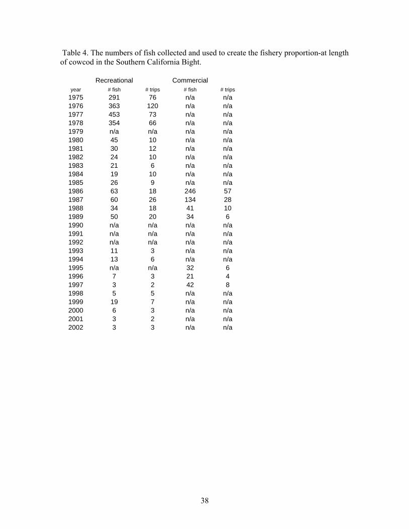
38

Table 4. The numbers of fish collected and used to create the fishery proportion-at length of cowcod in the Southern California Bight.

Recreational Commercial year # fish # trips # fish # trips

1975 291 76 n/a n/a 1976 363 120 n/a n/a 1977 453 73 n/a n/a 1978 354 66 n/a n/a 1979 n/a n/a n/a n/a 1980 45 10 n/a n/a 1981 30 12 n/a n/a 1982 24 10 n/a n/a 1983 21 6 n/a n/a 1984 19 10 n/a n/a 1985 26 9 n/a n/a 1986 63 18 246 57 1987 60 26 134 28 1988 34 18 41 10 1989 50 20 34 6 1990 n/a n/a n/a n/a 1991 n/a n/a n/a n/a 1992 n/a n/a n/a n/a 1993 11 3 n/a n/a 1994 13 6 n/a n/a 1995 n/a n/a 32 6 1996 7 3 21 4 1997 3 2 42 8 1998 5 5 n/a n/a 1999 19 7 n/a n/a 2000 6 3 n/a n/a 2001 3 2 n/a n/a 2002 3 3 n/a n/a

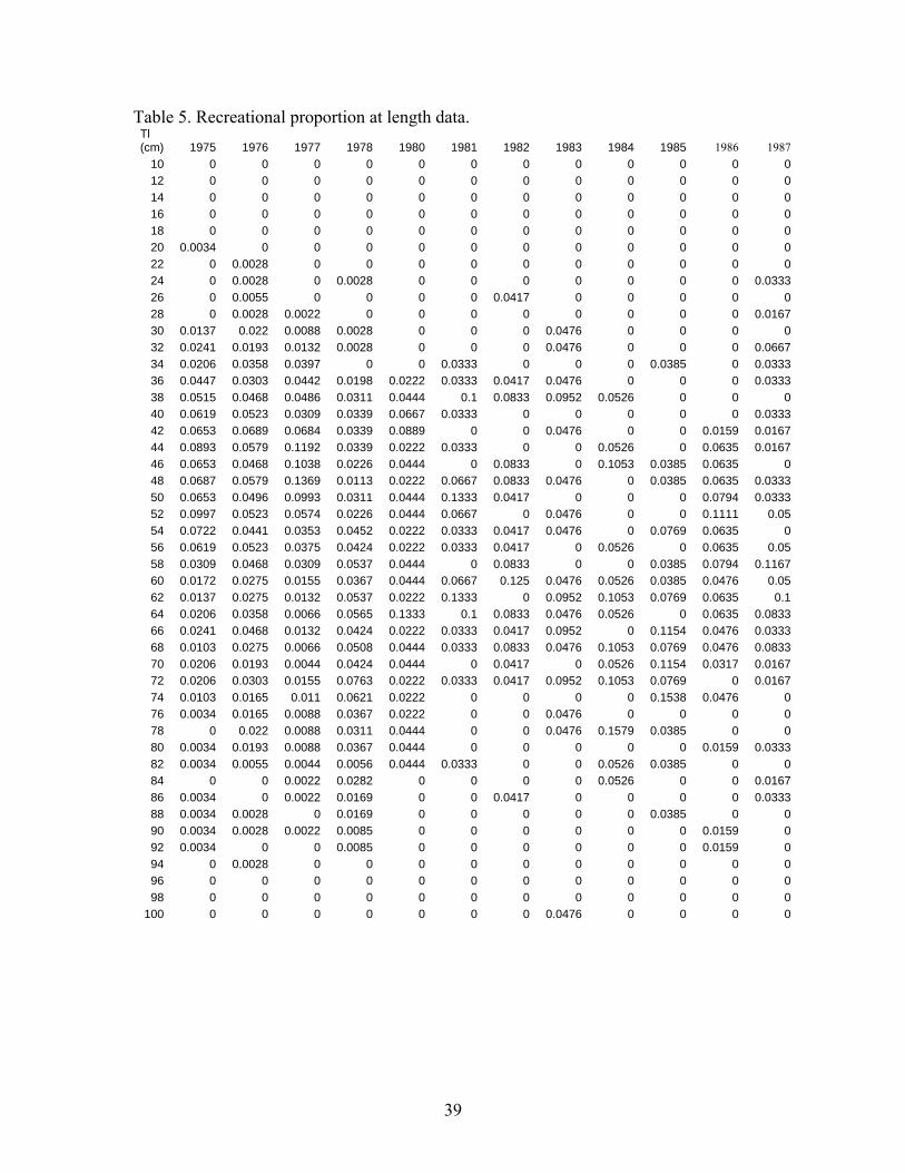
39

Table 5. Recreational proportion at length data. Tl (cm) 1975 1976 1977 1978 1980 1981 1982 1983 1984 1985 1986 1987

10 0 0 0 0 0 0 0 0 0 0 0 0 12 0 0 0 0 0 0 0 0 0 0 0 0 14 0 0 0 0 0 0 0 0 0 0 0 0 16 0 0 0 0 0 0 0 0 0 0 0 0 18 0 0 0 0 0 0 0 0 0 0 0 0 20 0.0034 0 0 0 0 0 0 0 0 0 0 0 22 0 0.0028 0 0 0 0 0 0 0 0 0 0 24 0 0.0028 0 0.0028 0 0 0 0 0 0 0 0.0333 26 0 0.0055 0 0 0 0 0.0417 0 0 0 0 0 28 0 0.0028 0.0022 0 0 0 0 0 0 0 0 0.0167 30 0.0137 0.022 0.0088 0.0028 0 0 0 0.0476 0 0 0 0 32 0.0241 0.0193 0.0132 0.0028 0 0 0 0.0476 0 0 0 0.0667 34 0.0206 0.0358 0.0397 0 0 0.0333 0 0 0 0.0385 0 0.0333 36 0.0447 0.0303 0.0442 0.0198 0.0222 0.0333 0.0417 0.0476 0 0 0 0.0333 38 0.0515 0.0468 0.0486 0.0311 0.0444 0.1 0.0833 0.0952 0.0526 0 0 0 40 0.0619 0.0523 0.0309 0.0339 0.0667 0.0333 0 0 0 0 0 0.0333 42 0.0653 0.0689 0.0684 0.0339 0.0889 0 0 0.0476 0 0 0.0159 0.0167 44 0.0893 0.0579 0.1192 0.0339 0.0222 0.0333 0 0 0.0526 0 0.0635 0.0167 46 0.0653 0.0468 0.1038 0.0226 0.0444 0 0.0833 0 0.1053 0.0385 0.0635 0 48 0.0687 0.0579 0.1369 0.0113 0.0222 0.0667 0.0833 0.0476 0 0.0385 0.0635 0.0333 50 0.0653 0.0496 0.0993 0.0311 0.0444 0.1333 0.0417 0 0 0 0.0794 0.0333 52 0.0997 0.0523 0.0574 0.0226 0.0444 0.0667 0 0.0476 0 0 0.1111 0.05 54 0.0722 0.0441 0.0353 0.0452 0.0222 0.0333 0.0417 0.0476 0 0.0769 0.0635 0 56 0.0619 0.0523 0.0375 0.0424 0.0222 0.0333 0.0417 0 0.0526 0 0.0635 0.05 58 0.0309 0.0468 0.0309 0.0537 0.0444 0 0.0833 0 0 0.0385 0.0794 0.1167 60 0.0172 0.0275 0.0155 0.0367 0.0444 0.0667 0.125 0.0476 0.0526 0.0385 0.0476 0.05 62 0.0137 0.0275 0.0132 0.0537 0.0222 0.1333 0 0.0952 0.1053 0.0769 0.0635 0.1 64 0.0206 0.0358 0.0066 0.0565 0.1333 0.1 0.0833 0.0476 0.0526 0 0.0635 0.0833 66 0.0241 0.0468 0.0132 0.0424 0.0222 0.0333 0.0417 0.0952 0 0.1154 0.0476 0.0333 68 0.0103 0.0275 0.0066 0.0508 0.0444 0.0333 0.0833 0.0476 0.1053 0.0769 0.0476 0.0833 70 0.0206 0.0193 0.0044 0.0424 0.0444 0 0.0417 0 0.0526 0.1154 0.0317 0.0167 72 0.0206 0.0303 0.0155 0.0763 0.0222 0.0333 0.0417 0.0952 0.1053 0.0769 0 0.0167 74 0.0103 0.0165 0.011 0.0621 0.0222 0 0 0 0 0.1538 0.0476 0 76 0.0034 0.0165 0.0088 0.0367 0.0222 0 0 0.0476 0 0 0 0 78 0 0.022 0.0088 0.0311 0.0444 0 0 0.0476 0.1579 0.0385 0 0 80 0.0034 0.0193 0.0088 0.0367 0.0444 0 0 0 0 0 0.0159 0.0333 82 0.0034 0.0055 0.0044 0.0056 0.0444 0.0333 0 0 0.0526 0.0385 0 0 84 0 0 0.0022 0.0282 0 0 0 0 0.0526 0 0 0.0167 86 0.0034 0 0.0022 0.0169 0 0 0.0417 0 0 0 0 0.0333 88 0.0034 0.0028 0 0.0169 0 0 0 0 0 0.0385 0 0 90 0.0034 0.0028 0.0022 0.0085 0 0 0 0 0 0 0.0159 0 92 0.0034 0 0 0.0085 0 0 0 0 0 0 0.0159 0 94 0 0.0028 0 0 0 0 0 0 0 0 0 0 96 0 0 0 0 0 0 0 0 0 0 0 0 98 0 0 0 0 0 0 0 0 0 0 0 0

100 0 0 0 0 0 0 0 0.0476 0 0 0 0

40

Table 5 continued Recreational proportion at length continued 1988 1989 1993 1994 1996 1997 1998 1999 2000 2001 2002

0 0 0 0 0 0 0 0 0 0 0 0 0 0 0 0 0 0 0 0 0 0 0 0 0 0 0 0 0 0 0 0 0 0 0 0 0 0 0 0 0 0 0 0 0 0 0 0 0 0 0 0 0 0 0 0 0 0 0 0 0 0 0 0 0 0 0 0 0 0 0 0 0 0 0 0 0 0 0 0 0 0 0 0 0.0526 0 0 0 0 0 0 0 0 0 0 0 0 0 0 0 0.04 0 0 0 0.3333 0.2 0 0 0 0 0 0.02 0 0 0 0 0 0 0 0.3333 0

0.0294 0.02 0 0 0.1429 0 0 0.0526 0 0.3333 0 0.0588 0.06 0 0 0.1429 0 0 0.1053 0 0 0 0.0588 0.02 0 0 0 0 0 0 0 0 0

0 0 0 0 0 0 0 0 0 0 0 0 0.08 0.0909 0 0.1429 0 0 0.0526 0 0 0

0.0588 0.08 0 0 0 0 0.2 0 0 0 0 0.0588 0.02 0 0 0.1429 0 0 0 0 0 0 0.0294 0.04 0 0 0 0 0.2 0 0 0 0 0.0588 0 0.0909 0.0769 0 0 0 0 0 0 0 0.0588 0 0 0.0769 0 0 0 0.0526 0 0 0 0.0588 0 0 0.0769 0 0.3333 0.2 0.0526 0 0 0.3333

0 0.04 0 0.1538 0 0 0 0 0 0 0 0.0294 0.04 0 0 0 0 0 0.0526 0 0.3333 0

0 0.04 0.0909 0 0.1429 0 0 0.2105 0 0 0 0.0294 0.06 0 0 0 0 0 0.0526 0.1667 0 0 0.0294 0.04 0 0 0 0 0 0.0526 0.1667 0 0 0.0294 0.04 0.1818 0.0769 0 0 0 0.1053 0 0 0 0.1471 0.02 0.3636 0 0 0 0 0.1579 0 0 0.3333 0.0882 0.04 0.1818 0.0769 0.1429 0.3333 0.2 0 0.3333 0 0

0 0.06 0 0.0769 0 0 0 0 0 0 0 0.0294 0.06 0 0.2308 0 0 0 0 0 0 0.3333

0 0.04 0 0.0769 0 0 0 0 0 0 0 0.0588 0.02 0 0.0769 0 0 0 0 0.3333 0 0 0.0588 0.02 0 0 0.1429 0 0 0 0 0 0

0 0.06 0 0 0 0 0 0 0 0 0 0.0294 0 0 0 0 0 0 0 0 0 0

0 0 0 0 0 0 0 0 0 0 0 0 0.02 0 0 0 0 0 0 0 0 0 0 0 0 0 0 0 0 0 0 0 0 0 0 0 0 0 0 0 0 0 0 0 0 0 0 0 0 0 0 0 0 0 0 0 0 0 0 0 0 0 0 0 0 0 0 0 0 0 0 0 0 0 0 0 0 0 0.02 0 0 0 0 0 0 0 0 0 0 0 0 0 0 0 0 0 0 0 0

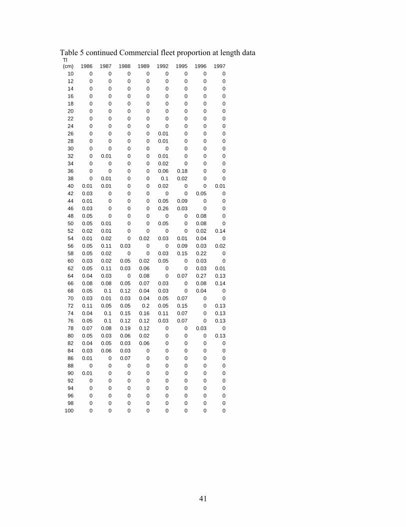
41

Table 5 continued Commercial fleet proportion at length data Tl (cm) 1986 1987 1988 1989 1992 1995 1996 1997

10 0 0 0 0 0 0 0 0 12 0 0 0 0 0 0 0 0 14 0 0 0 0 0 0 0 0 16 0 0 0 0 0 0 0 0 18 0 0 0 0 0 0 0 0 20 0 0 0 0 0 0 0 0 22 0 0 0 0 0 0 0 0 24 0 0 0 0 0 0 0 0 26 0 0 0 0 0.01 0 0 0 28 0 0 0 0 0.01 0 0 0 30 0 0 0 0 0 0 0 0 32 0 0.01 0 0 0.01 0 0 0 34 0 0 0 0 0.02 0 0 0 36 0 0 0 0 0.06 0.18 0 0 38 0 0.01 0 0 0.1 0.02 0 0 40 0.01 0.01 0 0 0.02 0 0 0.01 42 0.03 0 0 0 0 0 0.05 0 44 0.01 0 0 0 0.05 0.09 0 0 46 0.03 0 0 0 0.26 0.03 0 0 48 0.05 0 0 0 0 0 0.08 0 50 0.05 0.01 0 0 0.05 0 0.08 0 52 0.02 0.01 0 0 0 0 0.02 0.14 54 0.01 0.02 0 0.02 0.03 0.01 0.04 0 56 0.05 0.11 0.03 0 0 0.09 0.03 0.02 58 0.05 0.02 0 0 0.03 0.15 0.22 0 60 0.03 0.02 0.05 0.02 0.05 0 0.03 0 62 0.05 0.11 0.03 0.06 0 0 0.03 0.01 64 0.04 0.03 0 0.08 0 0.07 0.27 0.13 66 0.08 0.08 0.05 0.07 0.03 0 0.08 0.14 68 0.05 0.1 0.12 0.04 0.03 0 0.04 0 70 0.03 0.01 0.03 0.04 0.05 0.07 0 0 72 0.11 0.05 0.05 0.2 0.05 0.15 0 0.13 74 0.04 0.1 0.15 0.16 0.11 0.07 0 0.13 76 0.05 0.1 0.12 0.12 0.03 0.07 0 0.13 78 0.07 0.08 0.19 0.12 0 0 0.03 0 80 0.05 0.03 0.06 0.02 0 0 0 0.13 82 0.04 0.05 0.03 0.06 0 0 0 0 84 0.03 0.06 0.03 0 0 0 0 0 86 0.01 0 0.07 0 0 0 0 0 88 0 0 0 0 0 0 0 0 90 0.01 0 0 0 0 0 0 0 92 0 0 0 0 0 0 0 0 94 0 0 0 0 0 0 0 0 96 0 0 0 0 0 0 0 0 98 0 0 0 0 0 0 0 0

100 0 0 0 0 0 0 0 0

42

Table 6. Base Model Results. Columns are model and rows are likelihood and parameter values

Likelihood Component/ estimate

h=0.4 h=0.5 h=0.6

Likelihood compontents

Total Likelihood 12.91

13.43 14.03

CPFV CPUE 11.15 12.23 13.21

Visual survey 0.35 0.22 0.14

Parm priors 1.39 0.91 0.58

Parameter estmates

Ln (R0) 4.10 4.086 4.07

Initial F

CPFV CPUE q 0.0000149 .00000146 .00000143

Visual q 1.75 1.49 1.30

M (for all ages) 0.055 assumed 0.055 Assumed 0.055 Assumed

43

Table 7. Estimates of age 1+ biomass, spawning biomass, recruitment (age-0) and harvest rates and depletion (1914-2005) from all 3 levels of h.

h=0.4 h=0.5 h=0.6

year age 1+ bSpawnBio recruit-0 Hrate-1dep age 1+ bSpawnBio recruit-0 Hrate-1 dep age 1+ bSpawnBio recruit-0 Hrate-1 dep1914 3250 3101 60.7 -- 1.00 3191 3045 59.6 -- 1.00 3151 3007 58.8 -- 1.001915 3204 3055 60.7 0.000 0.99 3144 2998 59.6 0.000 0.98 3105 2961 58.8 0.000 0.981916 3204 3055 60.3 0.000 0.99 3144 2998 59.3 0.000 0.98 3105 2961 58.7 0.000 0.981917 3197 3049 60.3 0.001 0.98 3138 2992 59.3 0.001 0.98 3098 2954 58.6 0.001 0.981918 3186 3037 60.2 0.001 0.98 3126 2981 59.2 0.001 0.98 3087 2943 58.6 0.001 0.981919 3174 3025 60.1 0.000 0.98 3115 2969 59.2 0.000 0.98 3075 2931 58.6 0.000 0.971920 3167 3019 60.0 0.000 0.97 3108 2962 59.1 0.000 0.97 3069 2924 58.5 0.000 0.971921 3161 3012 60.0 0.000 0.97 3101 2955 59.1 0.000 0.97 3062 2918 58.5 0.000 0.971922 3155 3007 60.0 0.000 0.97 3096 2950 59.1 0.000 0.97 3057 2913 58.5 0.000 0.971923 3151 3003 59.9 0.000 0.97 3092 2946 59.1 0.000 0.97 3053 2909 58.5 0.000 0.971924 3146 2998 59.9 0.000 0.97 3087 2941 59.0 0.000 0.97 3047 2903 58.5 0.000 0.971925 3141 2993 59.9 0.000 0.97 3082 2937 59.0 0.000 0.96 3043 2899 58.5 0.000 0.961926 3135 2988 59.8 0.001 0.96 3076 2931 59.0 0.001 0.96 3037 2893 58.4 0.001 0.961927 3126 2979 59.7 0.001 0.96 3067 2922 58.9 0.001 0.96 3028 2884 58.4 0.001 0.961928 3119 2972 59.7 0.001 0.96 3060 2915 58.9 0.001 0.96 3021 2878 58.4 0.001 0.961929 3112 2965 59.6 0.001 0.96 3054 2909 58.9 0.001 0.96 3015 2871 58.4 0.001 0.951930 3106 2959 59.6 0.001 0.95 3048 2903 58.8 0.001 0.95 3009 2865 58.3 0.001 0.951931 3098 2951 59.5 0.001 0.95 3040 2895 58.8 0.001 0.95 3001 2858 58.3 0.001 0.951932 3091 2944 59.5 0.000 0.95 3032 2888 58.8 0.000 0.95 2994 2850 58.3 0.001 0.951933 3086 2939 59.4 0.000 0.95 3028 2883 58.7 0.000 0.95 2989 2846 58.3 0.000 0.951934 3083 2936 59.4 0.000 0.95 3025 2880 58.7 0.000 0.95 2987 2843 58.3 0.000 0.951935 3080 2933 59.4 0.000 0.95 3022 2878 58.7 0.000 0.95 2984 2841 58.3 0.000 0.941936 3077 2930 59.4 0.000 0.94 3020 2875 58.7 0.000 0.94 2982 2839 58.2 0.000 0.941937 3074 2928 59.3 0.000 0.94 3017 2873 58.7 0.000 0.94 2980 2836 58.2 0.000 0.941938 3072 2926 59.3 0.000 0.94 3015 2871 58.7 0.000 0.94 2978 2835 58.2 0.000 0.941939 3071 2925 59.3 0.000 0.94 3015 2871 58.7 0.000 0.94 2978 2835 58.2 0.000 0.941940 3070 2924 59.3 0.000 0.94 3015 2871 58.7 0.000 0.94 2978 2835 58.2 0.000 0.941941 3070 2924 59.3 0.000 0.94 3014 2870 58.7 0.000 0.94 2978 2835 58.2 0.000 0.941942 3069 2923 59.3 0.000 0.94 3014 2870 58.7 0.000 0.94 2978 2835 58.2 0.000 0.941943 3072 2926 59.3 0.000 0.94 3017 2873 58.7 0.000 0.94 2981 2839 58.2 0.000 0.941944 3072 2926 59.3 0.001 0.94 3018 2874 58.7 0.001 0.94 2982 2840 58.2 0.001 0.941945 3066 2920 59.3 0.001 0.94 3013 2869 58.7 0.001 0.94 2977 2834 58.2 0.001 0.941946 3048 2903 59.1 0.001 0.94 2995 2851 58.6 0.001 0.94 2960 2817 58.2 0.001 0.941947 3034 2889 59.0 0.001 0.93 2982 2838 58.5 0.001 0.93 2947 2804 58.1 0.001 0.931948 3024 2879 59.0 0.001 0.93 2972 2829 58.4 0.001 0.93 2938 2795 58.1 0.001 0.931949 3016 2871 58.9 0.001 0.93 2965 2821 58.4 0.001 0.93 2930 2788 58.1 0.001 0.931950 3007 2861 58.8 0.001 0.92 2956 2812 58.3 0.001 0.92 2922 2779 58.0 0.001 0.921951 2993 2848 58.7 0.001 0.92 2943 2799 58.3 0.001 0.92 2909 2767 58.0 0.001 0.921952 2977 2831 58.6 0.002 0.91 2927 2783 58.2 0.002 0.91 2894 2751 57.9 0.002 0.911953 2953 2808 58.4 0.002 0.91 2904 2760 58.1 0.002 0.91 2871 2728 57.8 0.002 0.911954 2929 2784 58.2 0.003 0.90 2880 2737 57.9 0.003 0.90 2848 2705 57.7 0.003 0.901955 2890 2745 57.8 0.004 0.89 2842 2698 57.7 0.004 0.89 2809 2667 57.6 0.004 0.891956 2833 2689 57.4 0.004 0.87 2786 2643 57.4 0.004 0.87 2754 2612 57.4 0.004 0.871957 2772 2627 56.8 0.004 0.85 2725 2582 57.0 0.004 0.85 2693 2551 57.1 0.004 0.851958 2718 2574 56.3 0.004 0.83 2672 2529 56.7 0.004 0.83 2641 2499 56.9 0.004 0.831959 2668 2524 55.9 0.004 0.81 2622 2479 56.3 0.004 0.81 2592 2450 56.7 0.004 0.811960 2626 2482 55.5 0.004 0.80 2581 2438 56.1 0.004 0.80 2550 2409 56.5 0.004 0.801961 2580 2437 55.0 0.003 0.79 2535 2393 55.8 0.003 0.79 2506 2364 56.3 0.004 0.791962 2545 2402 54.7 0.003 0.77 2501 2359 55.5 0.003 0.77 2472 2330 56.1 0.004 0.771963 2511 2369 54.4 0.003 0.76 2468 2327 55.3 0.004 0.76 2439 2298 55.9 0.004 0.761964 2478 2337 54.0 0.003 0.75 2436 2295 55.1 0.003 0.75 2408 2267 55.8 0.003 0.751965 2450 2310 53.8 0.004 0.74 2409 2269 54.9 0.004 0.75 2382 2242 55.7 0.004 0.751966 2412 2273 53.4 0.007 0.73 2372 2233 54.6 0.007 0.73 2346 2206 55.5 0.007 0.731967 2333 2195 52.5 0.009 0.71 2294 2155 54.0 0.009 0.71 2268 2129 55.0 0.009 0.711968 2232 2096 51.4 0.007 0.68 2195 2057 53.2 0.007 0.68 2170 2031 54.5 0.007 0.681969 2166 2031 50.6 0.006 0.65 2130 1993 52.6 0.006 0.65 2106 1967 54.1 0.006 0.651970 2125 1991 50.2 0.008 0.64 2091 1954 52.3 0.008 0.64 2067 1930 53.8 0.008 0.641971 2057 1924 49.3 0.007 0.62 2024 1888 51.6 0.007 0.62 2002 1865 53.4 0.007 0.621972 2006 1874 48.7 0.011 0.60 1975 1840 51.2 0.011 0.60 1954 1817 53.0 0.011 0.601973 1918 1786 47.5 0.013 0.58 1888 1754 50.3 0.013 0.58 1868 1732 52.4 0.014 0.581974 1812 1682 46.1 0.017 0.54 1784 1651 49.2 0.017 0.54 1766 1630 51.6 0.018 0.541975 1679 1550 44.1 0.017 0.50 1653 1521 47.6 0.018 0.50 1636 1502 50.4 0.018 0.501976 1563 1436 42.3 0.023 0.46 1539 1408 46.2 0.024 0.46 1524 1390 49.3 0.024 0.461977 1417 1291 39.8 0.020 0.42 1395 1266 44.1 0.020 0.42 1381 1249 47.6 0.021 0.421978 1320 1197 38.0 0.018 0.39 1301 1173 42.6 0.018 0.39 1289 1157 46.4 0.019 0.381979 1251 1129 36.7 0.024 0.36 1234 1108 41.4 0.025 0.36 1224 1094 45.5 0.026 0.361980 1153 1034 34.7 0.027 0.33 1139 1015 39.7 0.028 0.33 1131 1002 44.1 0.029 0.331981 1056 940 32.6 0.019 0.30 1046 923 37.8 0.020 0.30 1040 912 42.5 0.020 0.301982 1014 901 31.7 0.032 0.29 1007 887 37.0 0.034 0.29 1003 877 41.9 0.034 0.291983 921 811 29.5 0.022 0.26 917 799 35.0 0.023 0.26 915 792 40.1 0.023 0.261984 885 779 28.7 0.047 0.25 885 770 34.3 0.049 0.25 886 765 39.5 0.050 0.251985 763 662 25.5 0.065 0.21 766 656 31.2 0.067 0.22 771 652 36.7 0.068 0.221986 624 528 21.4 0.091 0.17 631 525 27.1 0.093 0.17 638 524 32.9 0.095 0.171987 478 387 16.7 0.076 0.12 489 387 21.9 0.078 0.13 500 389 27.7 0.079 0.131988 414 327 14.5 0.091 0.11 429 331 19.5 0.092 0.11 443 335 25.3 0.092 0.111989 352 270 12.3 0.044 0.09 371 278 17.1 0.044 0.09 389 285 22.7 0.043 0.091990 350 272 12.4 0.037 0.09 373 283 17.3 0.036 0.09 395 294 23.2 0.036 0.101991 353 279 12.7 0.031 0.09 381 294 17.8 0.031 0.10 407 309 23.9 0.029 0.101992 358 289 13.0 0.041 0.09 391 309 18.5 0.039 0.10 422 328 24.9 0.037 0.111993 352 288 13.0 0.026 0.09 390 314 18.7 0.024 0.10 426 337 25.3 0.023 0.111994 358 300 13.5 0.039 0.10 402 331 19.5 0.036 0.11 443 359 26.4 0.034 0.121995 348 296 13.3 0.025 0.10 397 333 19.6 0.023 0.11 444 366 26.7 0.021 0.121996 350 304 13.6 0.029 0.10 405 346 20.2 0.026 0.11 457 385 27.5 0.023 0.131997 345 305 13.7 0.008 0.10 406 353 20.5 0.007 0.12 465 398 28.1 0.007 0.131998 359 323 14.4 0.003 0.10 426 378 21.5 0.003 0.12 492 428 29.4 0.003 0.141999 377 344 15.1 0.005 0.11 451 405 22.6 0.005 0.13 523 462 30.7 0.004 0.152000 392 359 15.7 0.004 0.12 472 426 23.5 0.003 0.14 551 490 31.7 0.003 0.162001 407 375 16.3 0.000 0.12 494 448 24.3 0.000 0.15 580 519 32.7 0.000 0.172002 426 394 16.9 0.000 0.13 520 473 25.2 0.000 0.16 613 550 33.7 0.000 0.182003 444 411 17.6 0.000 0.13 545 497 26.1 0.000 0.16 646 581 34.7 0.000 0.192004 461 428 18.1 0.000 0.14 569 520 26.9 0.000 0.17 678 612 35.6 0.000 0.202005 478 444 18.7 0.000 0.14 593 542 27.7 0.000 0.18 710 642 36.4 0.000 0.21

44

Table 8. Sensitivity analysis over a range of M, h, and transect survey q and CV. h 0.4 0.4 0.4 0.5 0.5 0.5 0.6 0.6 0.6 0.7 0.7 0.7 0.5 0.5 0.5M 0.045 0.055 0.065 0.045 0.055 0.065 0.045 0.055 0.065 0.045 0.055 0.065 0.055 0.055 0.055visual q 0.65 0.65 0.65 0.65 0.65 0.65 0.65 0.65 0.65 0.65 0.65 0.65 0.65 0.75 0.75CV on visual q 0.5 0.5 0.5 0.5 0.5 0.5 0.5 0.5 0.5 0.5 0.5 0.5 0.75 0.5 0.75 likelihood value total 13.12 13.501 14.27 13.258 13.91 15.12 13.41 14.43 15.87 13.65 14.88 16.74 13.1 13.43 12.85cpfv CPUE 10.59 11.208 12.61 10.92 12.27 13.94 11.52 13.24 15.08 12.13 14.08 16.11 12.16 12.23 12.15visual transect 0.5 0.456 0.31 0.466 0.311 0.195 0.376 0.222 0.09 0.286 0.11 0.07 0.08 0.22 0.058priors 2.02 1.82 1.24 1.82 1.3 0.98 1.5 0.97 0.6 1.2 0.68 0.5 0.85 0.97 0.64 derived quantity virgin spawn bio 3288 3103 2976 3208 3046 2917 3163 3008 2878 3135 2980 2853 3041 3045 3040ending spawn bio 446 464 556 475 546 684 541.4 644 774 593 742 892 535 564 5342005spwnbio/unfished 0.14 0.15 0.19 0.15 0.18 0.23 0.17 0.21 0.27 0.19 0.25 0.31 0.18 0.19 0.18est visual q 1.7 1.67 1.53 1.69 1.4 1.2 1.53 1.25 1.07 1.37 1.14 0.94 1.61 1.49 1.64

45

Table 9. Projections of OY (40-10 adjusted catch), age-1 biomass and depletion levels (40-10 adjusted) h=0.4 h=0.5 h=0.6

year Catch (t) age-1+ biomass depletion

(t) Catch (t) age-1+ biomass depletion

(t) Catch (t) age-1+ biomass depletion (t)

2007 7.3 509 0.15 12.2 640 0.19 17.0 773 0.23

2008 7.8 518 0.15 12.9 651 0.20 17.9 788 0.24

2009 8.2 525 0.16 13.5 661 0.20 18.7 802 0.24

2010 8.6 531 0.16 14.1 671 0.20 19.5 815 0.24

2011 9.0 537 0.16 14.7 680 0.20 20.2 828 0.25

2012 9.3 543 0.16 15.2 688 0.20 20.9 840 0.25

2013 9.7 548 0.16 15.6 696 0.21 21.6 852 0.25

2014 10.0 553 0.16 16.1 705 0.21 22.2 864 0.26

2015 10.2 558 0.16 16.5 713 0.21 22.7 875 0.26

2016 10.5 562 0.17 16.9 721 0.21 23.3 887 0.26

2017 10.7 567 0.17 17.3 729 0.22 23.8 898 0.27

46

Table 9 continued. Projections of ABC, age-1 biomass and depletion levels (not 40-10 adjusted)

H=0.4 H=0.5 H=0.6

Catch (t) age-1 biomass depletion Catch (t) age-1 biomass depletion Catch (t) age-1 biomass depletion

2007 15.8 509 0.15 19.1 639 0.19 22.3 773 0.23

2008 16.1 509 0.15 19.6 644 0.19 23.0 783 0.24

2009 16.4 508 0.15 20.0 647 0.19 23.6 792 0.24

2010 16.6 507 0.15 20.4 651 0.19 24.2 801 0.24

2011 16.7 505 0.15 20.7 654 0.19 24.7 809 0.24

2012 16.8 504 0.15 20.9 657 0.19 25.1 817 0.24

2013 16.9 502 0.15 21.1 660 0.20 25.5 825 0.25

2014 16.9 500 0.15 21.3 663 0.20 25.8 833 0.25

2015 16.9 499 0.15 21.4 666 0.20 26.2 841 0.25

2016 16.8 498 0.15 21.6 670 0.20 26.5 850 0.25

2017 16.8 497 0.15 21.7 674 0.20 26.7 858 0.25

47

Table 10 Table of estimated age 1+ biomass and depletion levels assuming 3 states of nature (h) and harvest (OY) predicted by those states of nature.

State of nature: Catch used in the model with

Management options: Catch derived from: Year catch(t)

Low resilience H=0.4 Prob=0.3

Medium resilience H=0.5 Prob=0.4

High resilience H=0.6 Prob=0.3

2007 7.3 509 0.15 639 0.19 773 0.232008 7.8 518 0.15 655 0.20 798 0.242009 8.2 525 0.16 670 0.20 821 0.252010 8.6 531 0.16 685 0.21 845 0.252011 9.0 537 0.16 699 0.21 868 0.262012 9.3 543 0.16 713 0.21 891 0.272013 9.7 548 0.16 727 0.22 914 0.272014 10.0 553 0.16 741 0.22 936 0.282015 10.2 558 0.16 754 0.22 959 0.29

Low resilience H=0.4

2016 10.5 562 0.17 768 0.23 982 0.302007 12.2 509 0.15 640 0.19 773 0.232008 12.9 512 0.15 651 0.20 793 0.242009 13.5 515 0.15 661 0.20 812 0.242010 14.1 516 0.15 671 0.20 831 0.252011 14.7 517 0.15 680 0.20 849 0.252012 15.2 517 0.15 688 0.20 866 0.262013 15.6 517 0.15 696 0.21 883 0.262014 16.1 516 0.15 705 0.21 900 0.272015 16.5 516 0.15 713 0.21 918 0.27

Medium resilience H=0.5

2016 16.9 515 0.15 721 0.21 935 0.282007 17.0 509 0.15 639 0.19 773 0.232008 17.9 508 0.15 646 0.19 788 0.242009 18.7 505 0.15 651 0.19 802 0.242010 19.5 502 0.15 656 0.20 815 0.242011 20.2 497 0.15 659 0.20 828 0.252012 20.9 492 0.14 663 0.20 840 0.252013 21.6 487 0.14 666 0.20 852 0.252014 22.2 481 0.14 668 0.20 864 0.262015 22.7 475 0.14 671 0.20 875 0.26

High resilience H=0.6

2016 23.3 468 0.14 673 0.20 887 0.26

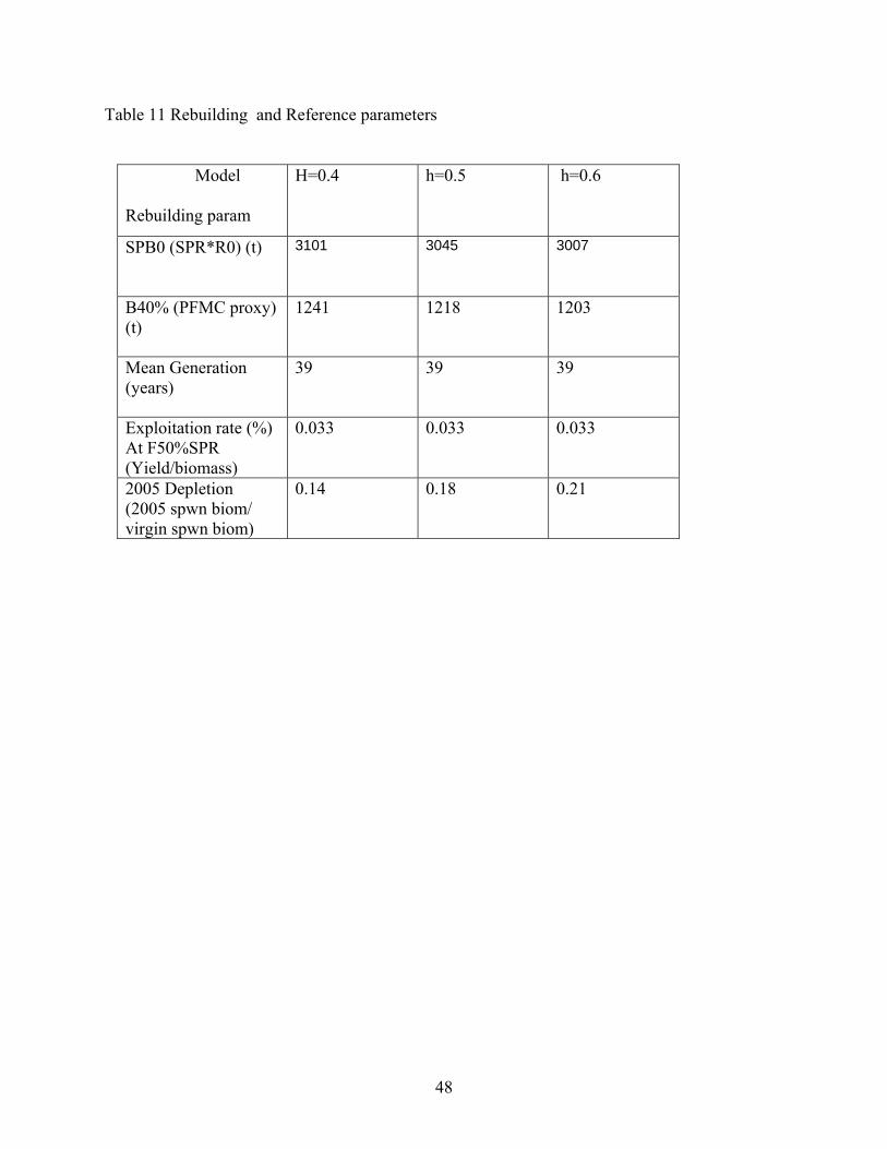
48

Table 11 Rebuilding and Reference parameters

Model Rebuilding param

H=0.4

h=0.5 h=0.6

SPB0 (SPR*R0) (t) 3101

3045

3007

B40% (PFMC proxy) (t)

1241 1218 1203

Mean Generation (years)

39 39 39

Exploitation rate (%) At F50%SPR (Yield/biomass)

0.033

0.033

0.033

2005 Depletion (2005 spwn biom/ virgin spwn biom)

0.14 0.18 0.21

49

Figure 1 Map of Pacific West Coast showing state, INPFC

Stock boundary

50

year

1920 1940 1960 1980 2000

catc

h (t)

50

100

150

200

250

Figure 2. The landing of cowcod in the Southern California Bight in the recreationaland commercial fleets. Black bars are commercial and grey bars recreational catches.

51

age (yrs)

0 10 20 30 40 50 60

TL

0

20

40

60

80

100

120

TL (cm)

20 40 60 80

prop

ortio

n m

atur

e

0.0

0.2

0.4

0.6

0.8

1.0

1.2

TL (cm)

0 20 40 60 80

kg

0

2

4

6

8

10

12

Figure 3. The length-at-age, maturity ogive and length weight relationships used in the cowcod stock assessment.

52

year

1940 1950 1960 1970 1980 1990 2000 2010

CPF

V %

pos

itive

inde

x

0.00

0.05

0.10

0.15

0.20

Figure 4. The proportion of tows estimated to be positive in the CalCOFI survey (1951-2003).New estimates are given with filled symbols and the previous assessments estimatesare depicted with open symbols.

year

1960 1970 1980 1990 2000

CP

FV C

PU

E in

dex

(sta

ndar

dize

d)

0.00

0.02

0.04

0.06

0.08

0.10

0.12

Figure 5. Estimate of the CPUE of the California Passanger Fishing Vessles 1961-2000.New estimates ( ) are plotted against the estimates from the previous assesment ( ).

year

1965 1970 1975 1980 1985 1990 1995 2000 2005

Out

fall

surv

ey %

pos

-10

0

10

20

30

40

50

Figure 6. The arithmetic estimate of the precentage of Las Angeles and Orange CountySanitation department tows that were positive 1973-2002.

53

RecFIN private boat

year

1975 1980 1985 1990 1995 2000

#fis

h/an

gle

day

0.00

0.02

0.04

0.06

0.08

0.10

Recfin Party Boat

year

1975 1980 1985 1990 1995 2000 2005

#fis

h/an

gle

day

0.00

0.02

0.04

0.06

0.08

Figure 7. Recreation CPUE series derived from the RecFIN database (1980-2000) for both the private boat and party boat (CPFV) fleets. Error bars are 1 SE.

54

1975

0.1

0.2

1976

1977

1978

1980

1981

20 40 60 80 100 120

1982

1983

1984

1985

1986

1987

20 40 60 80 100 120

1988

0.1

0.2

0.3

0.4

0.5

1993

1994

1996

1997

0 20 40 60 80 100120

1998

1999

2000

2001

2002

20 40 60 80 100120

1989

Figure 8. Length composition of cowcod in the recreational fleet operatingin the Southern California Bight 1975-present. Missing years indicated no samples.

55

1986Pr

opor

tion

0.1

0.2

1987

20 40 60 80 100 120

0.1

0.2

1988

0.1

0.2

1989

TL

0 20 40 60 80 100 120

0.1

0.2

1995

0.1

0.2

1996

0.1

0.2

1997

TL

0 20 40 60 80 100 120

0.1

0.2

Figure 9. The length compositon of the cowcod catch in the commercial fisheries in the Southern California Bight 1986- present. Many years have no sample information.

1992

0.1

0.2

56

Year

1970 1975 1980 1985 1990 1995 2000 2005

TL

20

30

40

50

60

70

80

90

Figure 10. The percentiles (10th, 50th and 90th) of the length distribution for commercial and recreational proportion at length data. Open symbols depict recreational data, and filled the commercial. Squares represent the10th percentile, circles the 50th and triangles the 90th.

57

year

1900 1920 1940 1960 1980 2000 2020

spaw

ning

bio

mas

s (t)

0

1000

2000

3000

4000

5000

6000

year

1900 1920 1940 1960 1980 2000 2020

age

1+ b

iom

ass

(t)

0

500

1000

1500

2000

2500

3000

3500

depl

etio

n

0.0

0.2

0.4

0.6

0.8

1.0

1.2

year

1900 1920 1940 1960 1980 2000 2020

age

0 re

crui

ts

0

20

40

60

80

100

year

1900 1920 1940 1960 1980 2000 2020

harv

est r

ate

(%)

0.00

0.05

0.10

0.15

0.20

Figure 11 h=0.4. Upper panel depicts spawning biomass (solid line) and estimated CPFV CPUE (circles) q adjusted. The second panel depicts age 1+ biomass (solid line) and q adjusted estimate of the visual transect survey (circle). Depletion level is given by the dashed line and corresponds to the right axis. The 3rd panel depicts age 0 recruitment. The 4th panel depicts the harvest rate.

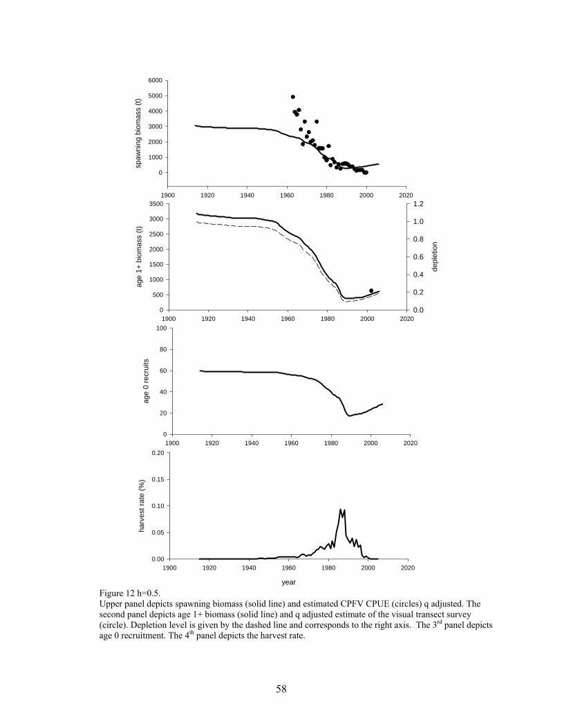
58

year

1900 1920 1940 1960 1980 2000 2020

spaw

ning

bio

mas

s (t)

0

1000

2000

3000

4000

5000

6000

year

1900 1920 1940 1960 1980 2000 2020

age

1+ b

iom

ass

(t)

0

500

1000

1500

2000

2500

3000

3500

depl

etio

n

0.0

0.2

0.4

0.6

0.8

1.0

1.2

year

1900 1920 1940 1960 1980 2000 2020

age

0 re

crui

ts

0

20

40

60

80

100

year

1900 1920 1940 1960 1980 2000 2020

harv

est r

ate

(%)

0.00

0.05

0.10

0.15

0.20

Figure 12 h=0.5. Upper panel depicts spawning biomass (solid line) and estimated CPFV CPUE (circles) q adjusted. The second panel depicts age 1+ biomass (solid line) and q adjusted estimate of the visual transect survey (circle). Depletion level is given by the dashed line and corresponds to the right axis. The 3rd panel depicts age 0 recruitment. The 4th panel depicts the harvest rate.

59

year

1900 1920 1940 1960 1980 2000 2020

spaw

ning

bio

mas

s (t)

0

1000

2000

3000

4000

5000

6000

year

1900 1920 1940 1960 1980 2000 2020

age

1+ b

iom

ass

(t)

0

500

1000

1500

2000

2500

3000

3500

depl

etio

n

0.0

0.2

0.4

0.6

0.8

1.0

1.2

year

1900 1920 1940 1960 1980 2000 2020

age

0 re

crui

ts

0

20

40

60

80

100

year

1900 1920 1940 1960 1980 2000 2020

harv

est r

ate

(%)

0.00

0.05

0.10

0.15

0.20

Figure 13 h=0.6. Upper panel depicts spawning biomass (solid line) and estimated CPFV CPUE (circles) q adjusted. The second panel depicts age 1+ biomass (solid line) and q adjusted estimate of the visual transect survey (circle). Depletion level is given by the dashed line and corresponds to the right axis. The 3rd panel depicts age 0 recruitment. The 4th panel depicts the harvest rate.

60

selectivity

TL (cm)

0 20 40 60 80 100

prop

ortio

n

0.0

0.2

0.4

0.6

0.8

1.0

Figure 14. The selectivity ogive from base case (same as female maturity).

61

Appendix 1

Updated ASSESSMENT- Delay Difference Model This reanalysis of the previous assessment method was designed to address the same two questions as the previous assessment. What is the current spawning biomass relative to historical or virgin levels? Is recruitment sufficient to maintain current catches? Furthermore a third question was addressed. Has the re-analysis of the times series (cpue series, CalCOFI, outfall, and catch) substantially changed the assessment results. This section of the assessment document is included to act as a bridge between the previous assessment model and the modeling presented in the next section. We do not intend for this modeling to be the basis for management decisions, but will base our recommendations on the SS2 assessment models. In this section, we show with the use of the previous model the effects of the new years of data on the population assessment method used previously. The exact same model formulation given by Butler et al. 1999 was used, and the description of the model as well as the ADMB code taken directly from Butler et al. (1999) is given in appendix 1.

Three data sources were used in this modeling effort. The CalCOFI (1951-2003) time series was used as an index of relative abundance of the fishable/spawning biomass. The CPFV CPUE series (1963-2000) was used as an index of relative abundance of the fishable/spawning biomass. The fishable biomass was made up of fish 40cm FL and larger. The 40 cm (FL) size was chosen as it approximates the knife edge cutoff between mature and immature fish. The Outfall survey was a recruitment index (1973-1998), with a seven year lag before recruiting to the fishable biomass. Individual recruitments (post 1950) were estimated as a random walk process.

The model for cowcod was broken in into two time periods. The “recent” period in the model was 1951-2005 and included all years with abundance information for cowcod (CalCOFI data begins in 1951). The “historical” period was 1916-1951 and included the year with catch but no abundance data. The assessment model for cowcod rockfish was a C++ program (calculations in double precision arithmetic) implemented using AD-Model Builder (Otter Software Ltd.). Parameters were estimated from the Hessian and the delta method by AD Model Builder’s AutoDIF library routines.

Model Results The first step in the analysis was to check if our use of the new data analysis (not including data post 1998) within the same dynamic model produced different results from the 1998 assessment (Butler et al. 1998). Comparison of spawning biomass trajectories show similarities but that the new catch data (~10% higher 1990-1998) scales the biomass trajectory higher (Appendix Figure 1). When we sequentially add in only one piece of data (new meaning new catch or new index method up to 1998), there is very little change with the ending ratio of spawning biomass/ unfished biomass ranging from 7-10% (Appendix Figure 1) which is nearly identical to the original assessment.

62

0

500

1000

1500

2000

2500

3000

3500

4000

4500

1915

1921

1927

1933

1939

1945

1951

1957

1963

1969

1975

1981

1987

1993

old assessmetn

add new catch

new catch+CalCOFI

new catch_CC+CPUE

newcatch+CC+CPUE+Outfall

Figure Appendix 1. The timeseries of fishable/spawning abundance from the DD model that covered the time period 1915-1998. Each series incorporates the updated or new analysis of information used in the previous assessment. Example new catch+ CalCOFi indicates that the model was run with the 2005 estimates of catch (1916-1997) and includes estimates of the reanalysis of the CalCOFI survey (1951-1997). Satisfied that the assessment model and data analysis up to 1998 are essentially the same as the previous assessment (with the exception of catch) we sequentially updated each time series through the most recent data point (Figure Appendix 2). The results of the update of the previous assessment indicated that the population is approximately 1.5 % of unfished with a spawning biomass near 50mt in the SCB. This is somewhat less than reported in 1998, but does not indicate further decline relative to the 1998 spawning biomass. The population has been stable to increasing since 1998 to present, which is to be expected as fishery removals have been largely eliminated. The smaller ratio of ending to unfished spawning biomass is a result of 3 low CPUE points at the end of the timeseries and the inability of the assessment model to incorporate potentially larger recruitment events towards the end of the time series. Also this assessment significantly downweights the CalCOFI series post 1980, thus the positive change in this series is largely ignored. The small changes between this assessment and the previous one are likely within the substantial noise of the data and we believe that the view of the population has not been changed from the last assessment, and that it is too early to monitor significant population change with this model. We do believe, however that the assessment is likely underestimating cowcod abundance in the most recent time period. Abundance of 50 t seems unlikely and the model results of a fully age-structured analysis that indicates that the population is likely larger.

63

0

500

1000

1500

2000

2500

3000

3500

4000

4500

1915

1922

1929

1936

1943

1950

1957

1964

1971

1978

1985

1992

1999

post 98 catch

cat+CalCOFI

cat+CC+CPUE

cat+CC+cpue+outfall

Appendix Figure 2. The timeseries of fishable/spawning abundance from the DD model that covered the time period 1915-2005. Each series incorporates the updated or new analysis of information used in the previous assessment. Example new catch+ CalCOFi indicates that the model was run with the 2005 estimates of catch (1916-2005) and includes estimates of the reanalysis of the CalCOFI survey (1951-2003). Description of the delay difference model used by Butler et al. (1999) Population Dynamics Population dynamics calculations in the assessment model used Schnute’s (1985) delay-difference equation:

Bt+1 = (1 + p) Lt Bt - p Lt Lt-1 Bt-1+ Rt+1 - p Lt J Rt. where Bt was fishable (not total, see below) cowcod biomass in the SCB at the beginning of year t; p was Ford’s growth coefficient (see below); Lt=exp(-Zt)=exp[-(Ft+Mt)] was the fraction of the stock that survived in year t; Zt, Ft, and Mt were instantaneous rates for total, fishing and natural mortality; and Rt was the biomass of recruits at the beginning of year t. The term J = wk-1 / wk was the ratio of mean weight one year before recruitment (age k-1) and mean weight at recruitment (age k). Fishing mortality rates (Ft) were calculated from catch data and biomass based on Baranov’s catch equation and Sim’s (1982) algorithm.

Ford’s growth model:

wa =wk-1 + (wk - wk-1) (1 + p1+a-k) / (1-p) is mathematically the same as von Bertalanffy’s more familiar growth model Wa= Wmax [1 - exp(-K(a-tzero)] where Wmax, K and tzero are parameters. The Ford and Von Bertalanffy equations are the same (Schnute 1985) because Wmax = (wk - p wk-1)/(1-p), K = -ln(p) and tzero = ln[(wk - wk-1)/(wk - p wk-1)] / ln(p). There was too little information (i.e. no age composition data) to estimate year-to-year variation in recruitment as a series of independent annual recruitment parameters but, as described below, recruitment probably changed over time and trends in recruitment are important for cowcod. As described below, recruitment to the fishable stock in our model is made up of many age groups and, like a weighted

64

average, probably relatively smooth and consistent from year to year with extended periods of either higher or lower than average values. We chose an autocorrelated random walk approach to model annual recruitment variation for cowcod that accommodates these features:

teRtΩΡ=

where Ρ was average recruitment and Ωt was the sum of annual log-scale recruitment deviations ωi:

Recruitment deviations ωi were defined such that their sum (and average) over the whole time series (1950-1998) was zero. The delay-difference model gives the same results as more complicated age structured models if recruitment to stock is “knife-edged” at age k and occurs at the beginning of the year, natural mortality is the same for all age groups, and the Ford growth model holds. In Schnute’s (1985) original description of the delay-difference model, knife-edged recruitment means that fish recruit to the fishery en-masse on their kth birthday so that total biomass Bt includes all fish age k and older. These assumptions hold to varying degrees for cowcod (see below) but Butler et al. (1999) believed the data were insufficient to support a more complex and realistic model. Assumptions about knife-edged recruitment could be relaxed in the model for for cowcod because it tracks fishable biomass, rather than total biomass. Fishable biomass is the portion of total stock biomass that is fully vulnerable to fishing mortality. This has an important implications related to interpreting selectivity patterns and interpreting model results. Firstly, recruitment in any year to the fishable stock includes cowcod of many ages. The actual age of recruiting fish and selectivity at age is irrelevant. It is not necessary to specify body weights at and prior to recruitment (parameters v and V in Schnute 1985), although it is necessary to specify the growth parameter J, which is a ratio of weights. They report that their approach reduces problems in specifying fishery selectivities at the cost of measuring fishable biomass in lieu of total biomass. See Butler et al. (1999) for more details. Historical Calculations Preliminary model runs, like the abundance data, all showed declining trends in SCB cowcod abundance but two distinctly different hypotheses explained the data almost equally well (see below). Under the “high initial biomass/low recruitment” hypothesis, the SCB cowcod stock was initially at a very high level and declined because average recruitment was very low (in extreme scenarios, even lower than losses to natural mortality). Under the alternative “lower initial biomass/higher fishing mortality” scenario, the cowcod stock was at a lower initial abundance level, recruitment was higher and the stock declined because catches exceeded recruitment (in extreme cases catch and recruitment were almost equal and the stock was composed almost entirely of new recruits). The purpose of historical calculations was to help choose between these alternate extreme hypotheses. The purpose of historical calculations was to identify a plausible model, develop a picture of trends in the cowcod stock during historical years (1916-1950), and provide a way for managers to compare current stock size to the virgin condition. Historical biomass calculations use average recruitment to estimate a “near virgin” biomass level (see below) in the SCB during 1916. Near-virgin biomass is fished down during the historical period (based on historical catches) to a biomass level at the beginning of the recent period (1951) and trend that matches abundance data for the recent period. Thus, average recruitment

Ωt

= ωii = 1950

tℜ

65

from the model and historical catch data are the links used to choose a model with plausible near-virgin, historical and recent biomass estimates. Historical calculations are based on Stock Reduction Analysis (Kimura and Tagart 1982; Kimura et al. 1984; Kimura 1985). Butler et al.(1998) used a similar idea for blackgill rockfish (S. melanostomus). Model runs covering the historical period (1916-1950) assumed a constant level of average recruitment prior to 1951 (Rhist) that was estimated (by constraint, see below) in the model. Constant recruitment was assumed during the historical period because there was no historical abundance information to use in estimating recruitment trends. The first step in historical modeling was to calculate virgin biomass for SCB cowcod as equilibrium biomass from the delay-difference equation given constant historical recruitment Rhist and no fishing. The second step was to calculate near-virgin biomass as the equilibrium biomass given constant recruitment Rhist and a constant level of historical fishing mortality Fhist. Near virgin biomass was a crude proxy for B1916 (cowcod biomass in the first year with catch data) and used to start the delay-difference model for the historical period. Fhist was set at a low level based on preliminary runs and inspection of trends in catch after 1916. The third step was to use estimates of near virgin biomass (B1916), recruitment (Rhist) and catch data in the delay difference model to calculate biomass and fishing mortality during the historical period, 1916-1951. As described below, a constraint was used to make sure biomass estimates from historical and recent calculations for 1951 agreed and to link the two series of estimates. Parameters From Auxiliary Data The natural mortality rate (M) in for cowcod was assumed to be the same for all ages and years in the model. We used a range of values for M (0.04-0.07 y-1) for sensitivity analysis and the mid-range value 0.055 y-1 for basecase runs to accommodate uncertainty about this important parameter. The range used for modeling was lower than the range of total mortality rate estimates (0.055-0.087 y-1, see above) because the latter included some fishing mortality.

We used p=e-K=0.994 where K=0.00605 y-1 was the von Bertalanffy growth parameter for round weight and sexes combined (see above). For modeling, we assumed recruitment to the fishable stock in the SCB at about 40 cm FL or about 10 years of age (age estimate based on the Von Bertalanffy growth curves). As described above, age at recruitment is not very important in our model but the assumed size at recruitment might be because it effects calculation of a growth parameter J. Length composition data show that cowcod begin to recruit to commercial fishing gear used in SCB (set nets and hook-and-line gear) at about 30 to 40 cm FL or about 6-10 years of age (Figure 13). Length frequency data for CPFV trips (Figure 27) shows recruitment beginning at about 30 cm FL or about 6 years of age. Limited age composition data from the SCB shows recruitment to commercial and recreational fisheries at about 6-15 years of age. We calculated Jk=wk-1/wk for ages k=6-15 years based on the von Bertalanffy model (see below). For base case runs, we used J=0.811 (corresponding to k=10, the midpoint of the range). Sensitivity analysis (see below) was used to determine how this affected results. Age at Recruitment (k) J=wk-1/wk 6 0.179 10 0.811 15 0.905 Parameter Estimation and Tuning

66

The assessment model for cowcod included process and observation parameters. Process parameters control population dynamics and biomass calculations. Observation parameters are used to statistically compare trends in model results with trends in data. Process parameters estimated in the delay-difference model for cowcod were for recruitment (Ρ and ωt ) and initial biomass (B1951). Runs covering the historical period also estimated a parameter for average historical recruitment biomass (Rhist) and included an assumed equilibrium fishing mortality before 1916 (Fhist). Other process parameters (e.g. for growth and natural mortality) were estimated outside the assessment model. There were 53 parameters to estimate when the model was run with recent years only and 54 parameters to estimate when the model was run with historical years turned on. Most (49) were process parameters for recruitments during the recent period.

We tuned the assessment model for cowcod in the SCB to three abundance indices: 1) CPUE from CPFV logs; 2) CalCOFI proportion positive; and 3) LA&OCSD proportion positive tows (proportion positive bottom trawl tows). CPFV and CalCOFI data were assumed to measure relative abundance of the total fishable/spawning stock. As described above, these abundance indices were for SCB cowcod. LA&OCSD data were used as a recruitment index for cowcod. Recruitment to the fishable stock starts at about age ten (see above) so comparisons between data and model predictions were lagged by 10-3=7 years. For example, we compared recruitment of three-year-old cowcod in 1980 with model estimates of recruitment in 1987. LA&OCSD data were particularly important because they gave information about future recruitment. For example, data for 1993-1994 contain information about recruitment to the fishable stock in the years 2000-2001.

Predicted values for abundance indices were calculated:

tKtK BQI =∧

, where IK,t is abundance index kind K (either CPUE in units of fish h-1 or CalCOFI and LACSD in units of proportion) for year t, hats “^” denote model estimates, and QK is an observation parameter that converts from units of biomass to units of the abundance index. Goodness-of-fit for observed and predicted CPUE data was computed assuming log-normal measurement errors and the negative log-likelihood:

where NCPUE was the number of observations. Goodness of fit for proportions (CalCOFI and LACSD data) assumed binomial measurement errors. For example, the negative log-likelihood for CalCOFI of data was:

LCPUE = 0.05 LnICPUE

I∧

CPUE

⎛

⎝

⎜ ⎜

⎞

⎠

⎟ ⎟

2

I = 1

NCPUE∑

67

where A CalCOFI was a constant (see below), λCalCOFI was an assumed “effective” sample size (see below), and observed and predicted index values were proportions. In effect, the effective sample size was used as a weighting factor that determined how much emphasis was placed on CalCOFI data in the model (relative to CPUE and LACSD data and constraints, see below) in estimation of parameters. The constant for CalCOFI data was calculated:

where the dummy variable Di is one if 0 < ICalCOFI,i < 1 and zero otherwise. The constant depends only on the data (not the fit) and is the minimum possible log-likelihood (if observed and predicted values match exactly). It has no effect on biomass estimates but makes the adjusted log-likelihood (scaled likelihood) easier to interpret, plot and understand (Methot 1989). For simplicity, effective sample size was assumed constant for CalCOFI data during 1951-1986. Effective sample size for CalCOFI data during 1987-1998 was also constant but set at one-third the value for 1951-1986 to accommodate reductions in CalCOFI sampling effort (Hewitt 1988). Effective sample size for LA&OCSD data was constant in all years. We assumed that precision of the CalCOFI and LA&OCSD data as indices of abundance for cowcod would be less than expected based on sample size and and sampling theory (see below). This often occurs when binomial or multinomial proportions are used to monitor biological characteristics of fish stocks (e.g. age composition of catches) and sample size is large (Fournier and Archibald 1982).

As described above, effective sample sizes were set manually to single values in our model. Reasonable choices for effective sample size were approximated from the variance of residuals in a preliminary model run (Methot 1989). This “iterative re-weighting” approach was repeated once or twice until assumed and calculated values were roughly equal. For example, the expected variance of a predicted CalCOFI value based on standard formulas for proportions and n tows is:

( ) ( )y

pppVarλ

ˆ1ˆˆ −=

so that:

( )( )y

yyy pVar

pp ˆ1ˆ −=λ

The variance Var(py) of residuals in one year was calculated by using another, equivalent, standard formula:

LCalCOFI = −λCalCOFI ICalCOFI, i ln I∧

CalCOFI,i⎛

⎝ ⎜

⎞

⎠ ⎟ + 1− ICalCOFI,i

⎛ ⎝

⎞ ⎠ ln 1− I

∧CalCOFI,i

⎛

⎝ ⎜

⎞

⎠ ⎟

⎡

⎣ ⎢ ⎤

⎦ ⎥ − Ai = 1

NCalCOFI∑

⎧ ⎨ ⎩

⎫ ⎬ ⎭

A = Dii = 1

NCalCOFI∑ ICalCOFI, i ln ICalCOFI , i

⎛ ⎝

⎞ ⎠ + 1− ICalCOFI , i

⎛ ⎝

⎞ ⎠ ln 1 − ICalCOFI, i

⎛ ⎝

⎞ ⎠

⎡ ⎣

⎤ ⎦

68

( ) 222

)ˆ(21

)]ˆ1()1[()ˆ(yy

yyyyy pp

npppp

pVar −=−

−−−+−=

To estimate an effective sample size for the time series as a whole, we calculated the geometric mean (roughly equal to the median) of the effective sample sizes for each year:

Λ=eλ where Λ was the average log(λy) value.

Recruitment deviations were penalized based on changes between successive time steps:

where σ=0.5 was an assumed standard deviation. Likelihood components used to penalize model fits with absurdly high fishing mortality rates were calculated:

if Fy ≥3, zero otherwise

if Fy ≥3, zero otherwise Penalties on high F values were not important for cowcod and always zero except in sensitivity analysis with vary low biomass levels. The constraint used to make recent and historical recruitment calculations agree was calculated:

( )2195119515.0 BbLHB −=

where b1951 and B1951 were estimates of cowcod biomass from historical and recent calculations. Choice of average recruitment for historical calculations is important. For example, if Rhist was fixed at some very large value, then b1951 and B1951 would probably be too large. The constraint used to estimate historical recruitment was:

LF1 = 0.5 Fy − 3⎛ ⎝ ⎜ ⎞

⎠ ⎟

2

y = 1916

y = 1950∑

LF2 = 0.5 Fy − 3⎛ ⎝ ⎜ ⎞

⎠ ⎟

2

y = 1951

y = 1998∑

Lω =ω y − ω y−1( )

σ

⎡

⎣ ⎢ ⎢

⎤

⎦ ⎥ ⎥

2

y = 1951

1998∑

69

LHR = 0.5 Rhist − µ( )2

where µ was the average of recruitments for a user-specified range of years during the recent model period. It would have been possible to set Rhist=µ without using a constraint and in practice, Rhist and µ were usually equal. However, the constraint adds some flexibility because the model was able estimate Rhist values slightly different from µ to achieve a better bit between b1951 and B1951 without distorting fit to abundance data in recent years. In addition, the constraint contributes a degree of uncertainty that was captured in variance calculations. This is a topic for future research. After diagnostic and sensitivity runs based results for recent years only, we turned historical years on and made decisions about historical fishing mortality rates (Fhist) and years to use in calculating the constraint for historical recruitment (Rhist). The decisions, based on intermediate model runs and the data, were subjective but reasonable. The goal was to develop a set of historical and recent estimates that were plausible. Population dynamics and observation parameters estimated in the model were chosen to minimize the total negative log-likelihood:

HISTLFLFFLFLOCSDLALOCSDLACalCOFILCalCOFICPUELCPUE ++++++=Ξ 2211&& λλλλλλ ωω

where the λ’s were weighting factors (usually one). LHIST was the negative log-likelihood for historical calculations:

HRHRHBHBHIST LLL λλ += with weighting factors zero except in runs including historical biomass calculations.

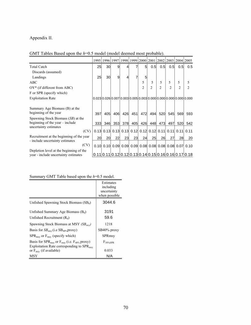
70

Appendix II. GMT Tables Based upon the h=0.5 model (model deemed most probable). 1995 1996 1997 1998 1999 2000 2001 2002 2003 2004 2005

Total Catch 25 30 9 4 7 5 0.5 0.5 0.5 0.5 0.5 Discards (assumed) Landings 25 30 9 4 7 5 ABC 5 5 5 5 5 5 OY* (if different from ABC) 2 2 2 2 2 2 F or SPR (specify which) Exploitation Rate 0.023 0.026 0.007 0.003 0.005 0.003 0.000 0.000 0.000 0.000 0.000 Summary Age Biomass (B) at the beginning of the year 397 405 406 426 451 472 494 520 545 569 593

333 346 353 378 405 426 448 473 497 520 542 Spawning Stock Biomass (SB) at the beginning of the year – include uncertainty estimates (CV) 0.13 0.13 0.13 0.13 0.12 0.12 0.12 0.11 0.11 0.11 0.11

20 20 22 23 23 24 25 26 27 28 20 Recruitment at the beginning of the year - include uncertainty estimates (CV) 0.10 0.10 0.09 0.09 0.09 0.08 0.08 0.08 0.08 0.07 0.10 Depletion level at the beginning of the year - include uncertainty estimates 0.11 0.11 0.12 0.12 0.13 0.14 0.15 0.16 0.16 0.17 0.18 Summary GMT Table based upon the h=0.5 model.

Estimates including

uncertainty when possible

Unfished Spawning Stock Biomass (SB0) 3044.6

Unfished Summary Age Biomass (B0)

3191 Unfished Recruitment (R0) 59.6

Spawning Stock Biomass at MSY (SBmsy) 1218 Basis for SBmsy (i.e SB40%proxy) SB40% proxy SPRmsy or Fmsy (specify which) SPRmsy Basis for SPRmsy or Fmsy (i.e. F40% proxy) F50%SPR Exploitation Rate corresponding to SPRmsy or Fmsy (if available) 0.033 MSY N/A

71

Appendix III. data and control file for cowcod h=0.5 Data file 1916 #start year 2006 # end year 1 12 1 #_spawn_seas 1 #_Nfleet 4 #_Nsurv fishery1%survey1%survey2%survey3%survey4 0.5 0.5 0.5 0.5 0.5#_surveytiming_in_season 1 #_Ngenders 80 #_Nages 2 #_init_equil_catch_for_each_fishery #_catch_biomass(mtons):_columns_are_fisheries,_rows_are_year*season 8.8 14.06 14.9 9.7 10.19 8.61 7.8 9.21 8.58 9.92 13.64 11.56 11.61 10.92 13.071 13.16 10.19 8.66 8.32 8.73 8.32 7.76 6.57 6.02 6.45 6.16 2.57 4.99 11.61 24.03 20.19 16.7 15.29 16.48 21.14 24.45 32.52 33.6 50.31 69.04 76.39 69.43 68.06 61.19 66.07 56.53 55.96 55.92 51.64 63 107.01 130.77 97.72 72.78

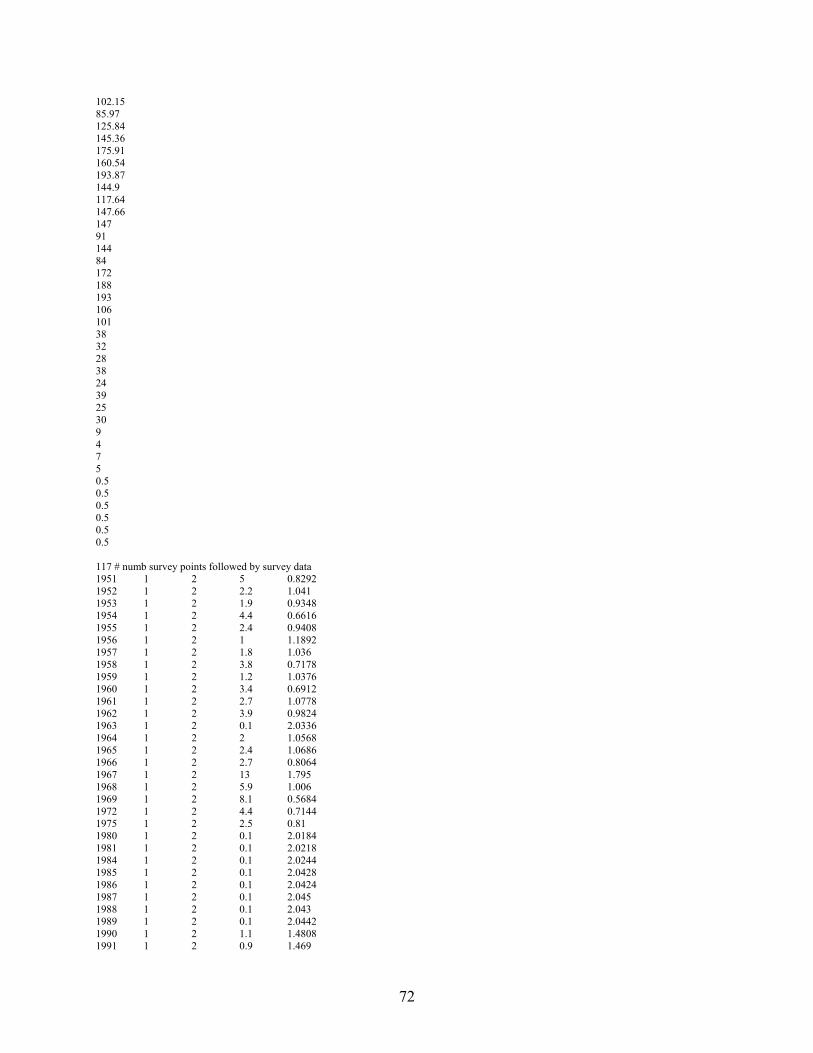
72

102.15 85.97 125.84 145.36 175.91 160.54 193.87 144.9 117.64 147.66 147 91 144 84 172 188 193 106 101 38 32 28 38 24 39 25 30 9 4 7 5 0.5 0.5 0.5 0.5 0.5 0.5 117 # numb survey points followed by survey data 1951 1 2 5 0.8292 1952 1 2 2.2 1.041 1953 1 2 1.9 0.9348 1954 1 2 4.4 0.6616 1955 1 2 2.4 0.9408 1956 1 2 1 1.1892 1957 1 2 1.8 1.036 1958 1 2 3.8 0.7178 1959 1 2 1.2 1.0376 1960 1 2 3.4 0.6912 1961 1 2 2.7 1.0778 1962 1 2 3.9 0.9824 1963 1 2 0.1 2.0336 1964 1 2 2 1.0568 1965 1 2 2.4 1.0686 1966 1 2 2.7 0.8064 1967 1 2 13 1.795 1968 1 2 5.9 1.006 1969 1 2 8.1 0.5684 1972 1 2 4.4 0.7144 1975 1 2 2.5 0.81 1980 1 2 0.1 2.0184 1981 1 2 0.1 2.0218 1984 1 2 0.1 2.0244 1985 1 2 0.1 2.0428 1986 1 2 0.1 2.0424 1987 1 2 0.1 2.045 1988 1 2 0.1 2.043 1989 1 2 0.1 2.0442 1990 1 2 1.1 1.4808 1991 1 2 0.9 1.469

73

1992 1 2 1 1.474 1993 1 2 0.1 2.0422 1994 1 2 0.1 2.038 1995 1 2 0.1 2.046 1996 1 2 0.1 2.0406 1997 1 2 0.1 2.0412 1998 1 2 0.1 2.0438 1999 1 2 1.04 1.478 2000 1 2 3.01 1.0828 2001 1 2 2.13 1.233 2002 1 2 0.1 2.0394 2003 1 2 4.53 0.913 1963 1 3 0.071542523 1.953799094 1964 1 3 0.05748274 1.689772189 1965 1 3 0.055060397 1.531356046 1966 1 3 0.059308434 1.214523761 1967 1 3 0.040768441 1.108912999 1968 1 3 0.027003596 1.003302237 1969 1 3 0.04826441 1.267329142 1970 1 3 0.03402068 1.320134523 1971 1 3 0.038283529 1.16171838 1972 1 3 0.029175205 1.531356046 1973 1 3 0.030455837 0.686469952 1974 1 3 0.026091295 0.686469952 1975 1 3 0.048316544 0.58085919 1976 1 3 0.023169089 0.58085919 1977 1 3 0.023090242 0.792080714 1978 1 3 0.02303154 1.689772189 1979 1 3 0.014366307 1.267329142 1980 1 3 0.011653262 0.58085919 1981 1 3 0.025012452 0.897691475 1982 1 3 0.007082721 1.003302237 1983 1 3 0.012855708 0.58085919 1984 1 3 0.009958842 0.58085919 1985 1 3 0.00483127 0.739275333 1986 1 3 0.007827743 0.792080714 1987 1 3 0.003787855 0.792080714 1988 1 3 0.008125175 1.16171838 1989 1 3 0.008527088 0.844886095 1990 1 3 0.008491133 0.844886095 1991 1 3 0.007241093 0.686469952 1992 1 3 0.005605051 0.950496856 1993 1 3 0.005826603 1.267329142 1994 1 3 0.003572569 0.739275333 1995 1 3 0.001900544 0.686469952 1996 1 3 0.002393212 0.686469952 1997 1 3 0.002533181 1.214523761 1998 1 3 0.002349113 1.16171838 1999 1 3 8.97E-05 1.372939904 2000 1 3 0.000148018 2.059409856 1970 1 4 12.5 2.285371046 1971 1 4 19.35483871 2.73011929 1972 1 4 28.125 3.106940109 1973 1 4 30 3.166703009 1974 1 4 8.771929825 1.9548323 1975 1 4 27.11864407 3.072132161 1976 1 4 3.636363636 1.29356403 1977 1 4 9.090909091 1.986575168 1978 1 4 1.785714286 0.915147308 1979 1 4 5.063291139 1.515064857 1980 1 4 4.938271605 1.497228298 1981 1 4 2.5 1.078872194 1982 1 4 1.234567901 0.763058197 1983 1 4 1.25 0.767752511 1984 1 4 2.43902439 1.065967165 1985 1 4 0.1 1.52026875 1986 1 4 6.097560976 1.653538081 1987 1 4 1.25 0.767752511 1988 1 4 3.75 1.312845714 1989 1 4 0.1 1.52026875

74

1990 1 4 1.25 0.767752511 1991 1 4 0.1 1.52026875 1992 1 4 0.1 1.52026875 1993 1 4 0.892857143 0.650041607 1994 1 4 2 0.96744375 1995 1 4 0.1 1.52026875 1996 1 4 1.25 0.767752511 1997 1 4 0.1 1.52026875 1998 1 4 0.1 1.52026875 1999 1 4 3.03030303 1.184564567 2000 1 4 10.84337349 2.148605632 2001 1 4 5.952380952 1.634996959 2002 1 4 3.296703297 1.233838337 2003 1 4 5.128205128 1.521949855 2004 1 4 1.282051282 0.77624685 2002 1 5 940 0.25 1 0 0 -1 0.0001 46 # len bins followed by begin of bin 10 12 14 16 18 20 22 24 26 28 30 32 34 36 38 40 42 44 46 48 50 52 54 56 58 60 62 64 66 68 70 72 74 76 78 80 82 84 86 88 90 92 94 96 98 100 26 #N_observations #Year Seas Fleet sexes Mkt Nsamp begin data: females then males 1975 1 1 0 0 76 0 0 0 0 0 0.003436426 0 0 0 0 0.013745704 0.024054983 0.020618557 0.04467354 0.051546392 0.06185567 0.065292096 0.089347079 0.065292096 0.068728522 0.065292096 0.099656357 0.072164948 0.06185567 0.030927835 0.017182131 0.013745704 0.020618557 0.024054983 0.010309278 0.020618557 0.020618557 0.010309278 0.003436426 0 0.003436426 0.003436426 0 0.003436426 0.003436426 0.003436426 0.003436426 0 0 0 0 1976 1 1 0 0 120 0 0 0 0 0 0 0.002754821 0.002754821 0.005509642 0.002754821 0.022038567 0.019283747 0.035812672 0.03030303 0.046831956 0.052341598 0.068870523 0.05785124 0.046831956 0.05785124 0.049586777 0.052341598 0.044077135 0.052341598 0.046831956 0.027548209 0.027548209 0.035812672 0.046831956 0.027548209 0.019283747 0.03030303 0.016528926 0.016528926 0.022038567 0.019283747 0.005509642 0 0 0.002754821 0.002754821 0 0.002754821 0 0 0 1977 1 1 0 0 73 0 0 0 0 0 0 0 0 0 0.002207506 0.008830022 0.013245033 0.039735099 0.04415011 0.048565121 0.030905077 0.068432671 0.119205298 0.103752759 0.136865342 0.099337748 0.057395143 0.035320088 0.037527594 0.030905077 0.015452539 0.013245033 0.006622517 0.013245033 0.006622517 0.004415011 0.015452539 0.011037528 0.008830022 0.008830022 0.008830022 0.004415011 0.002207506 0.002207506 0 0.002207506 0 0 0 0 0 1978 1 1 0 0 66 0 0 0 0 0 0 0 0.002824859 0 0 0.002824859 0.002824859 0 0.019774011 0.031073446 0.033898305 0.033898305 0.033898305 0.02259887 0.011299435 0.031073446 0.02259887 0.04519774 0.042372881 0.053672316 0.036723164 0.053672316 0.056497175 0.042372881 0.050847458 0.042372881 0.076271186 0.062146893 0.036723164 0.031073446 0.036723164 0.005649718 0.028248588 0.016949153 0.016949153 0.008474576 0.008474576 0 0 0 0 1980 1 1 0 0 10 0 0 0 0 0 0 0 0 0 0 0 0 0 0.022222222 0.044444444 0.066666667 0.088888889 0.022222222 0.044444444 0.022222222 0.044444444 0.044444444 0.022222222 0.022222222 0.044444444 0.044444444 0.022222222 0.133333333 0.022222222 0.044444444 0.044444444 0.022222222 0.022222222 0.022222222

75

0.044444444 0.044444444 0.044444444 0 0 0 0 0 0 0 0 0 1981 1 1 0 0 12 0 0 0 0 0 0 0 0 0 0 0 0 0.033333333 0.033333333 0.1 0.033333333 0 0.033333333 0 0.066666667 0.133333333 0.066666667 0.033333333 0.033333333 0 0.066666667 0.133333333 0.1 0.033333333 0.033333333 0 0.033333333 0 0 0 0 0.033333333 0 0 0 0 0 0 0 0 0 1982 1 1 0 0 10 0 0 0 0 0 0 0 0 0.041666667 0 0 0 0 0.041666667 0.083333333 0 0 0 0.083333333 0.083333333 0.041666667 0 0.041666667 0.041666667 0.083333333 0.125 0 0.083333333 0.041666667 0.083333333 0.041666667 0.041666667 0 0 0 0 0 0 0.041666667 0 0 0 0 0 0 0 1983 1 1 0 0 6 0 0 0 0 0 0 0 0 0 0 0.047619048 0.047619048 0 0.047619048 0.095238095 0 0.047619048 0 0 0.047619048 0 0.047619048 0.047619048 0 0 0.047619048 0.095238095 0.047619048 0.095238095 0.047619048 0 0.095238095 0 0.047619048 0.047619048 0 0 0 0 0 0 0 0 0 0 0.047619048 1984 1 1 0 0 10 0 0 0 0 0 0 0 0 0 0 0 0 0 0 0.052631579 0 0 0.052631579 0.105263158 0 0 0 0 0.052631579 0 0.052631579 0.105263158 0.052631579 0 0.105263158 0.052631579 0.105263158 0 0 0.157894737 0 0.052631579 0.052631579 0 0 0 0 0 0 0 0 1985 1 1 0 0 9 0 0 0 0 0 0 0 0 0 0 0 0 0.038461538 0 0 0 0 0 0.038461538 0.038461538 0 0 0.076923077 0 0.038461538 0.038461538 0.076923077 0 0.115384615 0.076923077 0.115384615 0.076923077 0.153846154 0 0.038461538 0 0.038461538 0 0 0.038461538 0 0 0 0 0 0 1986 1 1 0 0 75 0 0 0 0 0 0 0 0 0 0 0 0 0 0.003726109 0.002745554 0.005491107 0.023975823 0.025107231 0.039423332 0.050013325 0.059673047 0.038789742 0.022950011 0.051386102 0.055358606 0.03368583 0.056092765 0.048836659 0.075065245 0.051728039 0.026967772 0.084327719 0.038392493 0.034907754 0.050400521 0.040253034 0.031573867 0.023337206 0.005687218 0.002549443 0.01122861 0.006325836 0 0 0 0 1987 1 1 0 0 54 0 0 0 0 0 0 0 0.009169147 0 0.004584573 0 0.025235778 0.009169147 0.010376207 0.004828239 0.015721757 0.007343567 0.00596407 0.002414119 0.009514021 0.014169823 0.018581959 0.013967406 0.090315795 0.045886983 0.027203815 0.106483635 0.041201201 0.068487511 0.0960362 0.011826932 0.039416869 0.073458207 0.074837704 0.054835 0.030723785 0.033625236 0.045452168 0.009169147 0 0 0 0 0 0 0 1988 1 1 0 0 38 0 0 0 0 0 0 0 0 0 0 0 0.004063211 0.008126422 0.008126422 0 0 0.008126422 0.008126422 0.004063211 0.008126422 0.010961167 0.008126422 0 0.02620965 0 0.045964274 0.031259038 0.006897955 0.064431762 0.115303454 0.024981183 0.045964274 0.13004389 0.107696812 0.168820984 0.052442768 0.031613381 0.022146439 0.058378013 0 0 0 0 0 0 0 1989 1 1 0 0 26 0 0 0 0 0 0 0 0 0 0.012 0.006 0.006 0.018 0.006 0 0.024 0.024 0.006 0.012 0 0 0 0.025101604 0.012 0.012 0.031101604 0.053644385 0.066745989 0.058406417 0.038203209 0.046542781 0.159778075 0.121491979 0.086949198 0.08928877 0.031101604 0.041644385 0 0.006 0 0 0 0 0 0.006 0 1992 1 1 0 0 20 0 0 0 0 0 0 0 0 0.011688095 0.011688095 0 0.011688095 0.02337619 0.058440474 0.095842378 0.02337619 0 0.051427617 0.260310569 0 0.051427617 0 0.025713809 0 0.025713809 0.051427617 0 0 0.025713809 0.025713809 0.051427617 0.051427617 0.105860745 0.025713809 0.001502755 0 0.004508265 0 0.00300551 0.001502755 0.001502755 0 0 0 0 0 1993 1 1 0 0 3 0 0 0 0 0 0 0 0 0 0 0 0 0 0 0 0.090909091 0 0 0 0.090909091 0 0 0 0 0.090909091 0 0

76

0.181818182 0.363636364 0.181818182 0 0 0 0 0 0 0 0 0 0 0 0 0 0 0 0 1994 1 1 0 0 6 0 0 0 0 0 0 0 0 0 0 0 0 0 0 0 0 0 0 0 0.076923077 0.076923077 0.076923077 0.153846154 0 0 0 0 0.076923077 0 0.076923077 0.076923077 0.230769231 0.076923077 0.076923077 0 0 0 0 0 0 0 0 0 0 0 0 1995 1 1 0 0 6 0 0 0 0 0 0 0 0 0 0 0 0 0 0.177231565 0.015523933 0 0 0.089262613 0.028460543 0 0 0 0.012936611 0.086675291 0.147477361 0 0 0.07373868 0 0 0.07373868 0.147477361 0.07373868 0.07373868 0 0 0 0 0 0 0 0 0 0 0 0 1996 1 1 0 0 7 0 0 0 0 0 0 0 0 0 0 0 0.142857143 0.142857143 0 0 0.142857143 0 0.142857143 0 0 0 0 0 0 0.142857143 0 0 0 0 0.142857143 0 0 0 0 0.142857143 0 0 0 0 0 0 0 0 0 0 0 1997 1 1 0 0 10 0 0 0 0 0 0 0 0 0 0.333333333 0 0 0 0 0 0 0 0 0 0 0 0.333333333 0 0 0 0 0 0 0 0.333333333 0 0 0 0 0 0 0 0 0 0 0 0 0 0 0 0 1998 1 1 0 0 5 0 0 0 0 0 0 0 0 0 0.2 0 0 0 0 0 0 0.2 0 0.2 0 0 0.2 0 0 0 0 0 0 0 0.2 0 0 0 0 0 0 0 0 0 0 0 0 0 0 0 0 1999 1 1 0 0 7 0 0 0 0 0 0 0 0.052631579 0 0 0 0.052631579 0.105263158 0 0 0.052631579 0 0 0 0 0.052631579 0.052631579 0 0.052631579 0.210526316 0.052631579 0.052631579 0.105263158 0.157894737 0 0 0 0 0 0 0 0 0 0 0 0 0 0 0 0 0 2000 1 1 0 0 3 0 0 0 0 0 0 0 0 0 0 0 0 0 0 0 0 0 0 0 0 0 0 0 0 0 0.166666667 0.166666667 0 0 0.333333333 0 0 0 0.333333333 0 0 0 0 0 0 0 0 0 0 0 0 2001 1 1 0 0 2 0 0 0 0 0 0 0 0 0 0 0.333333333 0.333333333 0 0 0 0 0 0 0 0 0 0 0 0.333333333 0 0 0 0 0 0 0 0 0 0 0 0 0 0 0 0 0 0 0 0 0 0 2002 1 1 0 0 3 0 0 0 0 0 0 0 0 0 0 0 0 0 0 0 0 0 0 0 0 0 0.333333333 0 0 0 0 0 0 0.333333333 0 0 0.333333333 0 0 0 0 0 0 0 0 0 0 0 0 0 0 1973 1 4 0 0 98 0.50310559 0.086956522 0.062111801 0.093167702 0.062111801 0.055900621 0.043478261 0.037267081 0.037267081 0.01242236 0 0 0 0.00621118 0 0 0 0 0 0 0 0 0 0 0 0 0 0 0 0 0 0 0 0 0 0 0 0 0 0 0 0 0 0 0 0 36 #_N_age'_bins #_lower_age_of_age'_bins 1 2 3 4 5 6 7 8 9 10 11 12 13 14 15 20 21 22 23 24 25 26 27 28 29 30 35 40 45 50 55 60 65 70 75 80 0 #_number_of_ageerr_types #_vector_with_stddev_of ageing_precision_for_each_AGE_and_type 0 #_N_age_observations #Year Season Fleet Gender Mkt ageerr Lbin_lo Lbin_hi Nsamp 0 #_N_size@age_observations;_values_on_row1;_N_on_row2

77

#Year Season Fleet Gender Mkt ageerr Nsamp #_environmental_data 0 # N_variables 0 # N_observations #_Year Variable Value 999 #end of file Control File # no length information # visual survey treated as a relative index with prior 1 # num growth morphs 1 #assign sex to morph 1 #numb areas 1 1 1 1 1 #area for each fleet survey 0 #do migration 0 # numb blocks # mortality and growth parms 1 #last age for nat mortality young 2 #first age for nat mortality old 1 #age lmin 75 #age lmax -4 #MG parm dev phase #mortality and growth # lo hi init prior pr_type sd phase env-var use_dev dvmnyr dvmxyr dvsddv block blktype 0.01 0.1 0.055 0.055 0 0.8 -3 0 0 0 0 0.5 0 0 #M young 0 0 0 0 0 0.8 -3 0 0 0 0 0.5 0 0 #M old as exp offset 3 10 5 5 0 10 -3 0 0 0 0 0.5 0 0 #Lmin 80 99 90 90 0 0.8 -3 0 0 0 0 0.5 0 0 #Lmax 0.01 0.25 0.056 0.056 0 0.8 -3 0 0 0 0 0.5 0 0 #vbk 0.01 0.25 0.05 0.05 0 99 -4 0 0 0 0 0.5 0 0 #cv lmin 0 0.1 0 0 0 0.8 -3 0 0 0 0 0.5 0 0 #cv old as offset #len-wt and maturity -3 3 1.01E-05 1.01E-05 0 0.8 -3 0 0 0 0 0.5 0 0 #wt len -3 3 3.093 3.093 0 0.8 -3 0 0 0 0 0.5 0 0 # wt len2 -3 3 43 43 0 0.8 -3 0 0 0 0 0.5 0 0 #Maturity1 -3 3 -.64 -.64 0 0.8 -3 0 0 0 0 0.5 0 0 #Maturity 2 0 1 1 1 0 0.8 -3 0 0 0 0 0.5 0 0 #egg/gram 0 1 0 0 0 0.8 -3 0 0 0 0 0.5 0 0 #egg.gram slope #pop*growth morph for the prop of each morph in each area 0 1 1 1 0 0.8 -3 0 0 0 0 0.5 0 0 # fraction morph 1 to area 1 #pop lines for the prop assigned to each area 0 1 1 1 0 0.8 -3 0 0 0 0 0.5 0 0 # fraction to area 1 # cust env read 0 #custom block read 0 # lo hi init prior prtype sd phase #SR section 1 #1=beverton holt # lo hi init prior prtype sd phase 1 31 3.8 3.8 0 1000 1 # Ln(R0) 0.2 1 0.50 0.55 0 1000 -3 #Steepness

78

0 2 0.4 0.9 0 1000 -3 #sd recruitments -5 5 0 0 0 1 -3 #env link -5 5 0 0 0 1 -3 #init_eq 0 #index of environ variable to be used # start_rec end_rec Lower upper phase 2006 2005 -15 15 -3 #init_F # Lo Hi init prior prtype sd phase 0 .2 0.0001 0.0001 0 1000 1 #Qsetup #add param row for each positive entry below #float dopowe doenv dodev envvar numbio (1=biomass, 0=num) 0 0 0 0 0 1 1 0 0 0 0 0 1 0 0 0 0 0 1 0 0 0 0 1 1 0 0 0 0 1 #lo hi init prior prtype sd phase -50 50 -5 -5 0 1000 1 # float est for calcofi -50 50 -5 -5 0 1000 1 # float est for cpue -50 50 -5 -5 0 1000 1 # float est for outfall -50 50 -.274 -.274 0 0.5 1 # float est for visual #selex and retention #selextype doretention do male mirror 4 0 0 0 #fleet1 4 0 0 0 #survey1 4 0 0 0 #survey2 0 0 0 0 #survey3 0 0 0 0 #survey4 #age selex 10 0 0 0 #fleet 1 10 0 0 0 #survey2 10 0 0 0 #survey2 11 0 0 0 #survey4 10 0 0 0 #survey3 #LO HI INIT PRIOR PR_type SD PHASE env-variable use_dev dev_minyr dev_maxyr dev_stddev Block_Pattern #40 95 90 90 0 1000 -3 0 0 0 0 0.5 0 0 #peak #0.0001 0.2 0.001 .001 0 1000 -2 0 0 0 0 0.5 0 0 #init #-10 5 1.1 1.1 0 1000 2 0 0 0 0 0.5 0 0 #infl #0.001 5 .1 .1 0 1000 3 0 0 0 0 0.5 0 0 #slope #-5 10 5 5 0 1000 -3 0 0 0 0 0.5 0 0 #final #-10. 5 4 4 0 1000 -4 0 0 0 0 0.5 0 0 #infl2 #.001 5 0.09 0.09 0 1000 -5 0 0 0 0 0.5 0 0 #slope2 #0.1 20 12 12 0 1000 -4 0 0 0 0 0.5 0 0 #width of top #1 14 1 1 0 25 -99 0 0 0 0 0.5 0 0 # fleet 2 start mirror low #45 46 46 46 0 25 -99 0 0 0 0 0.5 0 0 #fleet 2 upper mirror 1 40 3 3 0 1000 -1 0 0 0 0 0.5 0 0 #minage 1 40 3 3 0 1000 -1 0 0 0 0 0.5 0 0 #maxage # custom env read 0 #custom block read 0 -4 # phase for selex parms dev 1 #max lambda phases 0 # include (1) or not (0) the constant offset for Logs(s) in the Log(like) calculation # survey lambdas 1 0.0001 1 0.0001 1 # discard lambdas

79

0 0 0 0 0 # mean body wt 0 #lenfreq lambda 0 0 0 0 0 #age freq lambda 0 0 0 0 0 # size at age 0 0 0 0 0 #init equlib catch 1 #rec lambda 1 #parm prior lambda 1 #prior dev timeseries lambda 0 #crashpen lambda 100 #max F .9999 999

80

Appendix IV. Expansion using CPFV

An expansion factor for the abundance of cowcod (Sebastes levis) in the Cowcod Conservation Areas, based on

estimates of habitat availability and recreational catch rates.

E.J. Dick, Alec MacCall and John Field NMFS SWFSC Santa Cruz Laboratory

April 2005 Introduction We develop an expansion factor for an estimate of cowcod abundance (Yoklavich et al., in press) in the Cowcod Conservation Areas (CCA), for use in the estimation of stock abundance in the Southern California Bight (U.S. waters south of Point Conception). The approach described in this document incorporates two primary sources of data: 1) logbook data from commercial passenger fishing vessels (CPFVs) and 2) area estimates of benthic habitat for cowcod in the region. Several sources of uncertainty exist for these data, some of which are unknown or can only be approximated. In addition, cowcod are relatively rare in the logbook data, with the vast majority of trips reporting no catch for this species. To obtain estimates of relative abundance inside and outside the CCA, we estimate the spatial distribution of catch rates (densities) using generalized linear models (GLMs), and then multiply density by the area of available cowcod habitat, which is calculated using Geographic Information System (GIS) software and maps of substrate types. Data and Methods Recreational (CPFV) Logbook Data The California Department of Fish and Game (CDFG) provided us with logbook data for the recreational fishery from 1980-2000. Data from previous years were not included since trip-specific information is unavailable, and the expansion factor should be derived from the state of the stock in recent years. Data from recent years were excluded due to the establishment of the CCA in 2001, which makes comparison of catch rates inside and outside the conservation area inappropriate. In 2000, a bag limit of 1 cowcod and 10 rockfish per landing took effect for recreational anglers in California, whereas in previous years cowcod were included in a 15-rockfish bag limit. To examine the effect of this bag limit on catch rates, we used data from RecFIN (http://www.psmfc.org/recfin/forms/bfreq.html) on the number of cowcod per angler bag over the time period 1980-2000. As in the previous assessment (Butler et al., 2002), only data from CDFG fishing blocks south of Point Conception and inside U.S. waters were retained (blocks 651-897), excluding blocks 600, 699, 700, 799, and 800, which represent data of uncertain location. To standardize the trips considered in our analysis, trips lasting less than 1 hour (0.02% of records) or greater than 12

81

hours (‘multi-day’ trips; <1% of total) were removed. Records with zero anglers or more than 60 anglers on a trip were also removed, which accounted for less than 5% of the total records. The logbook data contained individual records for each species caught, from which we defined trip-specific records as unique combinations of boat, day, month and year. The use of trip-specific records allowed us to examine the composition of catch on a given trip, which in turn provides information on whether a given trip should be considered fishing effort for cowcod. For each trip, we retained information on the catch of 30 species in addition to cowcod. These species were selected because they were relatively common in the historical CPFV database for southern California, or because they indicate trips that should be excluded from the analysis (e.g. benthic invertebrates suggest a dive trip). The presence or absence of each species in a given trip was then used as a binary predictor (‘dummy’ variable) in a multiple logistic regression model, with presence or absence of cowcod catch as the response variable (Stephens and MacCall, 2004). This model estimates, for each trip, the probability of catching a cowcod given the other species that were caught. Trips with low probabilities are those that target species that do not co-occur with cowcod (e.g. tuna trips), and trips with high probabilities are actual fishing effort for cowcod. The decision on which trips to include (a ‘cut-off’ probability) is based on the premise that including all trips increases the variance of the estimates by introducing ‘noise’ (trips targeting other species) into the data, while excluding too many trips increases the variance by reducing sample size. We selected a cut-off point by conducting a sensitivity analysis of the mean CV for block effects in the delta-GLM index of abundance (described below), selecting the cut-off probability that minimized the average CV. To examine the spatial distribution of catch rates (CPUE) in the SCB, we used a delta-GLM model of relative abundance (Stefansson, 1996). This method is useful for modeling catch rates when there are a large number of records with zero catch. The quantity of interest for this analysis is CPUE per CDFG block. The probability, πi, of catching a cowcod in block i was estimated using a binomial GLM with a probit link function

( ) βxTii =Φ − π1

where 1−Φ is the inverse of the cumulative standard normal distribution function. The probit link was selected over a logit link based on the Bayesian Information Criterion (see Results, Table 3a). The mean CPUE for block i, given that a trip caught a cowcod, was modeled as

( ) iTiiCPUE ε+= βxlog

where εi ~ N(0, σ2) and β is a vector of regression coefficients. The mean CPUE (µi) for block i, given that a cowcod was caught, was calculated by exponentiation with a bias correction term (σ2/2). The delta-GLM index of relative abundance is the product of the back-transformed block effects from the two models. Model selection was based on residual analyses and the Bayesian Information Criterion (BIC). Due to computational limitations, years were combined into 4 ‘group.year’ categories to permit investigation of interactions terms.

82

Standard errors for block effects were estimated using a jackknife routine. If we symbolize the delta-GLM function by ),,(ˆˆ

1 nXX Lθθ = , for n observations, and let

),,,,,(ˆˆ111)( niii XXXX LL +−= θθ ,

then the ‘jackknife mean’ is simply ∑=

• =n

i

i

n1

)()(

ˆˆ θ

θ

and the jackknife estimate of standard error is defined as

21

1

2)()( )ˆˆ(1ˆ ⎥

⎦

⎤⎢⎣

⎡−

−= ∑

=•

n

iiJ n

n θθσ .

Habitat Data Area estimates of suitable habitat for cowcod were calculated using GIS software (ArcView 3.2a). Digital maps (‘shapefiles’) of benthic habitat types were obtained from the Pacific Coast Groundfish Essential Fish Habitat Project (TerraLogic GIS, NMFS and PSMFC), which also included bathymetry data. CDFG provided spatial data for blocks and the perimeters of the CCA. Mary Yoklavich provided shapefiles of the submersible survey area as illustrated in Yoklavich et al. (in press). Habitat types in the Pacific Coast Groundfish Essential Fish Habitat (EFH) data are a generalized version of the data used to define the submersible survey area (Gary Greene, pers. comm.), but this was the only available habitat data that covered the entire SCB. We defined cowcod habitat as those habitat types in the EFH data that intersected the Yoklavich et al. survey area and fell within the approximate depths of the survey (75-300 m). Bathymetry data that were readily available and in the necessary format (polygon shapefiles) were in 10-meter increments. Therefore this analysis is based on cowcod habitat defined as suitable substrate types within the 70-300 meter depth contours. The habitat types in the EFH data which intersected the survey area maps from Yoklavich et al. are “rocky ridge,” “rocky shelf,” “rocky slope,” “sedimentary ridge,” “sedimentary shelf” and “sedimentary slope.” Since the relative densities of cowcod for these habitat classifications are unknown, we estimated the area of cowcod habitat in a given block as the sum of all habitat types. The highest densities of adult cowcod reported in Yoklavich et al. were for “43-fathom Bank” (inside the Eastern CCA). The EFH data classifies this general area as “sedimentary ridge.” Expansion Factor, Catchability Coefficient and Variance Estimator

The expansion factor is defined as the ratio CCAin abundancecowcodSCBin abundance cowcod .

83

Since the unit of spatial resolution for catch rates is CDFG fishing block, it is necessary to classify each block as ‘inside’ or ‘outside’ the CCA. A block that crosses the conservation area boundary is classified as ‘inside’ if the majority of cowcod habitat in that block falls within the CCA (see Results). This assumes that fishing only occurs the in areas defined as cowcod habitat. Abundances inside and outside the CCA were estimated as

( )( )i

n

iiInside HCPUEN ∑

=

=1

and ( )( )j

m

jjOutside HCPUEN ∑

=

=1

(1)

where CPUE is the estimated catch rate for a given block, H is the area (km2) of cowcod habitat in a block, n is the number of blocks classified as inside the CCA, and m is the number of blocks classified as outside the CCA. The expansion factor is therefore

Inside

Outside

Inside

OutsideInside

NN

NNNR +=

+= 1 (2)

Assuming no error in the area estimates and independence of the block effects in the delta-GLM model, the variance for abundance inside the CCA (and similarly for abundance outside) is

( )2

1i

n

iiInside HCPUEVarNVar ∑

=

= (3)

where VarCPUEi is estimated by the jackknife routine for the delta-GLM index. We used the delta method (Rice, 1995) to approximate the variance of the ratio InsideOutside NN , which equals VarR. Let X = NInside, Y = NOutside, and Z = Y / X. Then

⎟⎟⎠

⎞⎜⎜⎝

⎛−+≈

X

YYXY

X

YX

X

ZVarµµσρσσ

µµσ

µ21 2

2

22

2 (4)

Our estimate of VarR assumes that ρ = 0. Positive or negative correlations in abundance would decrease or increase the variance, respectively. If instead we wish to treat the expansion factor as a catchability coefficient (q), our expansion factor becomes

OutsideInside

Inside

NNN

q+

= (5)

The variances for inside and outside can again be estimated as in equation 3, and the delta method can approximate the variance of the ratio, as in equation 4.

84

Results and Discussion The bag frequency analysis from RecFIN (Table 1) suggests that the bag limit change for cowcod in 2000 should not have a significant effect on catch rates. While this provides an additional year of data, using the expansion factor still assumes no change in relative abundance inside versus outside the CCA between 2000 and 2003, the latter being the year of the submersible survey. The distributions of hours fished and number of anglers from the disaggregated CPFV logbook data (Figures 1 & 2) illustrate that trimming extreme values from the data, as described in the “Data and Methods” section, should isolate trips of interest and improve standardization of catch rates. Coefficients from the species regression model (Figure 3) illustrate how the presence or absence of species/groups in the reported catch is associated with the probability of catching a cowcod during a CPFV trip. The results are intuitive: species/groups that occupy deeper reefs (rockfish, lingcod, sablefish) have higher probabilities (more positive coefficients) of co-occurrence with cowcod, whereas most highly migratory and nearshore species have lower probabilities (more negative coefficients). Trips that were assigned a probability of greater than 0.12 were retained as ‘effective effort’ for cowcod, based on the results of the sensitivity analysis (Table 2). An additional 2,046 trips were deleted due to sparse data and the need to stabilize the jackknife routine in the delta-GLM model. These procedures reduced the number of trips in the database from 340,566 to 23,845 (effective effort for cowcod). Model selection for the delta-GLM index (binomial and Gaussian GLMs) indicated that a ‘main effects’ model containing block, ‘group.year’ and month terms was sufficient for estimating block-specific catch rates (Table 3). Given the large number of records and model parameters, investigation of interaction terms required grouping of years into 4 categories (‘group years’). This was based on the year effects from the delta-GLM index (Figure 4), and resulted in 4 groups: 1980-1985, 1986-1991, 1992-1997, and 1998-2000. Months were retained in the Gaussian GLM to allow for estimation of delta-GLM month effects. The delta-GLM index estimated block effects for 97 out of 221 blocks in the SCB (Figure 5). Blocks were classified as ‘inside’ or ‘outside’ the CCA, according to the distribution of habitat inside each block (Figure 5). Habitat types inside the CCA contain a greater proportion of rocky substrate than habitat outside (Table 4). The sum of all habitat area in the SCB divided by the area of habitat in the CCA is 2.72, which can be interpreted as an expansion factor based solely on habitat availability. The expansion factor, R, (Eq. 2) based on estimates of catch rates from 1980 to 2000 and habitat area is 1.55, with an approximate standard error of 0.0655 (the square root of Eq. 4). Treating this factor as a catchability coefficient, q, (Eq. 5) provides an estimate of 0.645, with an approximate standard error of 0.082. At the request of the stock assessment review (STAR) panel, the final expansion factor was calculated using data from 1990 to 2000. The model structure was unchanged (i.e. model 2 in Table 3a and model 1 in Table 3b) and this subset of the data allowed for estimation of 62 block

85

effects (Figure 6). The final expansion factor is 1.33 (Eq. 2) with an approximate standard error of 0.064. Expressing the factor as a catchability coefficient, q, (Eq. 5) produces an estimate of 0.751 with a standard error of 0.147. As mentioned above, this analysis cannot account for several major sources of uncertainty (inaccuracies in logbook data, uncertainty in classification of habitats, etc.). Recognition of the uncertainty in components of the model that are presently treated as being without variability would almost certainly produce higher estimates of the standard errors. References Butler, J.L., L.D. Jacobson, J.T. Barnes, H.G. Moser. 2002. Biology and population dynamics of cowcod (Sebastes levis) in the Southern California Bight. Fishery Bulletin 101(2):260-280. Rice, J.A. 1995. Mathematical Statistics and Data Analysis, 2nd Ed. Duxbury Press, 602 pp. Stefansson, G. 1996. Analysis of groundfish survey abundance data: Combining the GLM and delta approaches. ICES Journal of Marine Science 53(3): 577-588. Stephens, A. and A. MacCall. 2004. A multispecies approach to subsetting logbook data for purposes of estimating CPUE. Fisheries Research, 70: 299-310. TerraLogic GIS; National Marine Fisheries Service, Northwest Region; Pacific States Marine Fisheries Commission. ca. 2002. Pacific Coast Groundfish Essential Fish Habitat Project; Consolidated GIS Data, Vol. 1; Physical and Biological Habitat. Contacts: TerraLogic GIS and Steve Copps, NMFS Yoklavich, M., M. Love, and K. Forney. (in press) A fishery independent assessment of cowcod (Sebastes levis) in Southern California’s Cowcod Conservation Areas using direct observations from an occupied submersible. [draft 12/1/2004]

86

Tables Table 1: Bag frequency analysis, 1980-1999 (RecFIN). 2000 results shown for comparison.

Year 0 1 2 3 5 6 7 Total Bags1980 12 5 1 2 2 1 1 241981 4 22 1 1 281982 9 11 1 211983 9 15 1 251984 10 16 261985 5 15 2 1 231986 5 8 131987 1 11988 2 21989 1 11993 3 1 41994 1 8 91995 1 11996 1 1 21997 1 11998 3 31999 6 8 1 15

(2000)* 4 3 7Total Bags, 80-99 65 118 7 5 2 1 1 199

Cumulative % 32.7% 92.0% 95.5% 98.0% 99.0% 99.5% 100.0%* bag limit of 1 cowcod

Bag Size

Table 2: Sensitivity analysis for the ‘cut-off probability’ in the species-regression model. The cut-off probability that minimized the mean CV of the delta-GLM block effects was used to determine which records were ‘effective effort’ for cowcod.

cut-off probability Mean CV of block effects in delta-GLM number of records0.10 34.92% 285130.11 34.92% 285120.12 34.68% 258910.13 48.15% 68460.14 48.75% 68000.15 48.75% 6792

87

Table 3: Model selection for the delta-GLM index (binomial and Gaussian GLMs). a) Binomial GLM (23,845 records) Link Function Parameters BIC BIC difference*

1 cpue (0/1) = block + group.year + month logit 111 18846 272 cpue (0/1) = block + group.year + month probit 111 18819 03 cpue (0/1) = group.year + month probit 15 20964 21454 cpue (0/1) = block + month probit 108 19170 3515 cpue (0/1) = block + group.year probit 100 18830 116 cpue (0/1) = block + group.year + month + block:group.year probit 399 20472 1653

* "BIC difference" is the BIC value minus the smallest BIC value in the set of candidate models

b) Gaussian GLM (3,948 records) Link Function Parameters BIC BIC difference1 loge(cpue) = block + group.year + month identity 111 11556 222 loge(cpue) = group.year + month identity 15 11572 383 loge(cpue) = block + month identity 108 11565 304 loge(cpue) = block + group.year identity 100 11534 05 loge(cpue) = block + group.year + month + block:group.year identity 399 12537 1003

c) Probability Distribution for Positive Observations Parameters AIC AIC difference1 Lognormal# 111 -17956 02 Gamma 111 -17107 849

# Identical to model 1 in part (b), but fit using a lognormal likelihood function for cpue, rather than a gaussian likelihood for log(cpue) Table 4: Habitat types inside and outside the CCA.

Habitat Type Area (km2) Proportion of Habitat Area (km2) Proportion of HabitatRocky Ridge 730.51 0.294 19.42 0.005Rocky Shelf 25.16 0.010 344.38 0.081Rocky Slope 15.11 0.006 311.37 0.073

Sedimentary Ridge 704.83 0.284 201.13 0.047Sedimentary Shelf 422.03 0.170 2526.54 0.591Sedimentary Slope 588.26 0.237 868.62 0.203

Inside CCA Outside CCA

88

Figures Figure 1: Distribution of hours fished in the disaggregated (1 record per species) CPFV logbook data for Southern California.

Reported Number of Hours Fished (1980-2000)

0

50000

100000

150000

200000

250000

300000

350000

400000

450000

1 11 21 32 46 70 84

Number of Hours Fished

Freq

uenc

y

0.0

0.1

0.2

0.3

0.4

0.5

0.6

0.7

0.8

0.9

1.0

1.1

cumulative proportion

Figure 2: Distribution of the number of anglers in the disaggregated (1 record per species) CPFV logbook data for Southern California.

Reported Number of Anglers (1980-2000)

0

10000

20000

30000

40000

50000

60000

1 11 21 31 41 51 61 71 81 91 101 111 121 131 141 158 201 535

Number of Anglers

Freq

uenc

y

0.0

0.2

0.4

0.6

0.8

1.0

cumulative proportion

89

Figure 3: Coefficients from the logistic regression model for the probability of catching cowcod. Positive and negative coefficients represent higher and lower probabilities, respectively, that a species/group co-occurs with cowcod in the CPFV logbook data.

-10 -8 -6 -4 -2 0 2 4

rockfish, unspecified

kelp bass

Pacific bonito

Pacific mackerel

barracuda

rock bass

barred sand bass

CA Scorpionfish

halfmoon

CA Halibut

Yellowtail

ocean whitefish

white croaker

sheephead

albacore tuna

white seabass

jack mackerel

lingcod

flounder, unspecified

sole, unspecified

sablefish

cabezon

skipjack tuna

sandab, unspecified

yellowfin tuna

bluefin tuna

regression coefficients

90

Figure 4: Estimated year effects from the binomial GLM (upper panel), Gaussian GLM (middle panel), and delta-GLM index (lower panel). Vertical lines in the lower panel separate groups of years in the final model.

1980 1985 1990 1995 2000

0.15

0.20

0.25

0.30

0.35

Year

Pr p

ositiv

e tri

p

1980 1985 1990 1995 2000

0.03

50.

045

0.05

5

Year

Mea

n C

PUE

| pos

itive

trip

1980 1985 1990 1995 2000

0.00

50.

010

0.01

50.

020

Year

Del

ta-G

LM In

dex

91

Figure 5: Distribution of cowcod habitat and catch rates (1980-2000) by CDFG fishing block in the Southern California Bight. Block effects are categorized by quartiles.

Figure 6: Distribution of cowcod habitat and catch rates (1990-2000) by CDFG fishing block in the Southern California Bight. Block effects are categorized by

92

quartiles.

93

Appendix V.

The use of CalCOFI larval abundance data to derive an expansion factor for the estimated abundance of cowcod (Sebastes levis) inside the Cowcod Conservation Areas

John Field, Alec MacCall and Edward Dick, April 29 2005 Introduction The objective of this addendum to the cowcod assessment is to present a potential expansion factor for scaling the cowcod (Sebastes levis) biomass estimates generated by Yoklavich et al. (in prep) in order to reflect plausible biomass levels throughout the Southern California Bight. As described by Moser et al. (2000), cowcod larvae are among the few rockfish larvae easily identified to species in California Cooperative Oceanic Fisheries Investigations (CalCOFI) ichthyoplankton dataset. They are also among the rarest of those larvae identifiable to species, with a total of 550 larvae counted in 117 positive tows in the standard survey area between 1951 and 1998 (Moser et al. 2000). The low frequency of positive tows, and small number of larvae overall, suggests that any inference about the abundance, particularly of relative abundance by area, based on such data is tenuous. Nevertheless, a reasonable approach to doing so is attempted here. General Approach Our basic approach used generalized linear models to estimate the relative density of cowcod larvae both inside and outside of the Cowcod Conservation Areas (CCAs), expanded the density by the relative area sampled both inside and outside of the CCAs, and used the ratio between the two to derive a possible expansion factor for Yoklavich et al’s point estimate of biomass within the CCAs. The first significant assumption is that larval density is linearly proportional to adult abundance (spawning biomass). Although this is a difficult assumption to judge, it is reasonable based on Mangel and Smith’s (1990) observation that at low encounter rates, the proportion of positive tows for sardine eggs seemed to be strongly correlated with population biomass levels. Additionally, these data have already been used as abundance indices for cowcod (Butler et al. 1999). Consequently, we feel that this assumption is reasonable. The second major assumption is that cowcod larvae are caught in reasonably close proximity to the location of parturition, and consequently represent adult densities in the general locality of their capture. MacGregor (1986) presented length frequency compositions of rockfish larvae from CalCOFI samples, and found that 70% of S. levis larvae were within one millimeter of the expected size of newly hatched larvae, suggesting that a large proportion of captured larvae were spawned during the month of capture. He interpreted the decrease in numbers of larvae of larger sizes to reflect both high natural mortality rates and increasing net avoidance behavior with time. This would suggest that larvae tend to be caught in reasonable proximity to the area of parturition.

94

Yet presumably currents, eddies and other physical features are capable of dispersing larvae over substantial distances over short time periods. Consequently, the extent to which larval numbers in tows within and outside of the CCA may actually represent reproductive effort in these respective areas is uncertain. A third assumption regards the use of the enhanced CalCOFI survey data. The enhanced CalCOFI survey grid includes roughly 75 stations that were sampled in February of 2002 and 2003 (data since 2003 are not yet available). Nearly all of these stations are within the boundaries of the CCAs. The majority of these stations were not sampled prior to 2002, and consequently treating them as the relative equivalent to the usual CalCOFI stations may be questionable. However, this additional data represents a valuable source of information, therefore we have generated expansion factors both with and without the enhanced survey data. Data and Methods Moser et al. (2000) found that the highest numbers of cowcod were captured at the cluster of stations in the northern Channel Islands, with 68% of occurrences and 76% of the total numbers in an area bounded by lines 80 and 87 and seaward to station 55. As larvae were rare north of Point Conception and seaward of station 60, only data from CalCOFI lines 80-93, and stations seaward to station 60, were used in this analysis. This is similar to the approach used in the 1999 assessment. Several of the stations within the boundaries of the western CCA include those with the highest frequency of occurrence over time, particularly 87.40, 87.45 and 87.50, which had 24 of the 29 positive tows in the CCA over this time period. The other regular CalCOFI stations in the CCA are stations 90.45, 90.53, and 93.35; the latter is the only station to fall within the boundaries of the eastern CCA. For continuity, stations were assigned as inside or outside of the CCA based on their average coordinates over the time series. As the locations of tows may vary by a kilometer or more, a small number of the tows taken from stations considered inside the CCA may have actually been taken outside the CCA boundaries. Figure 1 shows the location of the standard CalCOFI stations used in this exercise (grey) and the enhanced cowcod survey stations (black). The size of the circles for the traditional stations reflects the average (Jan-June) CPUE for cowcod, and the number to the left of each station reflects the number of positive tows over the entire time series. For enhanced stations, triangles reflect positive stations (small were positive one year, large were positive both years), crosses reflect stations with no larvae either year. The CCAs and the effective CalCOFI sampling area are also outlined. The effective CalCOFI sampling area was estimated using boundaries connected by the shoreward stations, extending seaward equidistant between the stations included in this analysis and the next-nearest station (note- this could be improved upon by using the landward boundary, although this should not have a notable impact on the result). Using this approach, the total area of the CalCOFI region was determined to be 75,600 km2, and the area of the CCAs (inside) estimated at 13,700 km2, leaving 61,900 km2 as the area sampled outside the CCAs. Figure 2 reflects the paucity of data with which to consider current

95

differences in the relative density of cowcod inside and outside of the CCAs, as it shows the same larval catch information as Figure 1 for the years 1996-2003 only. In addition to inferred patchiness, larvae are typically most abundant during winter months, with 45% of spawning apparently occurring in January and another 39% in February and March (MacGregor 1986), such that only 4 tows produced larvae between July and December. Consequently only tows taken from January-June were used here, again consistent with the 1999 assessment. Rather than use months as independent factors, we used three-month periods (January-March, April-June) to reflect the quarterly nature of the majority of CalCOFI survey effort over time. Additionally, as the time series is generally considered to be noisy, with high frequency variability that is not likely to reflect actual changes in adult spawning biomass, the years of data collection were binned into five year periods to decrease the number of coefficients used in the models. Table 1 shows the estimated proportions of positive tows and of CPUE inside and outside of the CCA in five year intervals, and figure 3 shows the information in Table 1 graphically. To evaluate the potential differences in both presence/absence and abundance of cowcod larvae among stations inside and outside of the CCAs, we ran both binomial generalized linear models (GLMs) using presence/absence data, and a Delta-GLM (which combines a binomial model with a model of catch per unit effort for positive tows) to estimate the relative differences in larval densities inside and outside of the CCAs. The coefficients evaluated were inside or outside the CCAs, five-year intervals of time, and seasons (Jan-March, April-June). The GLM analyses was executed in R programming language using a procedure developed by E.J. Dick, which allows for evaluation of alternative distributions and a variety of diagnostics, and includes a jackknife estimation of precision. The appropriate probability distributions were diagnosed using Akaike Information Criteria (AIC), as in Dick (2004). Based on the results of the diagnostics, a logit link was used for the binomial model, and (where relevant) a lognormal distribution was used for the positive (Delta-GLM) model. The binomial component of the model generally explained a reasonable fraction of the variance as determined by AIC criteria. The positive component of the model improved the fit, but AIC shows the improvement to be insufficient. In general, the effects of including the factors of inside or outside the CCA, season, and five year intervals in the models improved the model performance, although the amount of variability explained was never substantial. To develop the expansion factor, we scaled the relative abundance of cowcod larvae by the respective area inside and outside of the CCA in the southern California Bight. The expansion factor was thus estimated as the ratio of the sum total of larvae (relative abundance, as indicated by percentage of positive tows) inside and outside the CCAs over the total number inside the CCAs, which simplifies to:

Eq. 1: ii

oo

DADA

E += 1

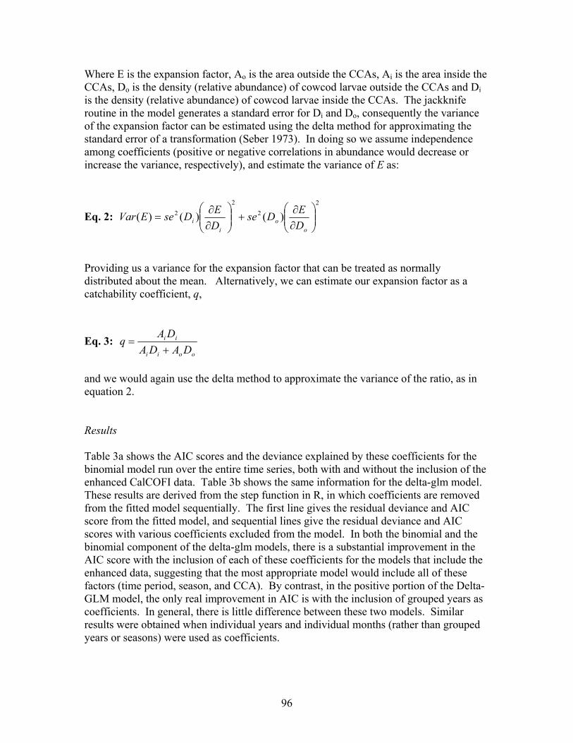
96

Where E is the expansion factor, Ao is the area outside the CCAs, Ai is the area inside the CCAs, Do is the density (relative abundance) of cowcod larvae outside the CCAs and Di is the density (relative abundance) of cowcod larvae inside the CCAs. The jackknife routine in the model generates a standard error for Di and Do, consequently the variance of the expansion factor can be estimated using the delta method for approximating the standard error of a transformation (Seber 1973). In doing so we assume independence among coefficients (positive or negative correlations in abundance would decrease or increase the variance, respectively), and estimate the variance of E as:

Eq. 2: 2

22

2 )()()( ⎟⎟⎠

⎞⎜⎜⎝

⎛∂∂

+⎟⎟⎠

⎞⎜⎜⎝

⎛∂∂

=o

oi

i DEDse

DEDseEVar

Providing us a variance for the expansion factor that can be treated as normally distributed about the mean. Alternatively, we can estimate our expansion factor as a catchability coefficient, q,

Eq. 3: ooii

ii

DADADA

q+

=

and we would again use the delta method to approximate the variance of the ratio, as in equation 2. Results Table 3a shows the AIC scores and the deviance explained by these coefficients for the binomial model run over the entire time series, both with and without the inclusion of the enhanced CalCOFI data. Table 3b shows the same information for the delta-glm model. These results are derived from the step function in R, in which coefficients are removed from the fitted model sequentially. The first line gives the residual deviance and AIC score from the fitted model, and sequential lines give the residual deviance and AIC scores with various coefficients excluded from the model. In both the binomial and the binomial component of the delta-glm models, there is a substantial improvement in the AIC score with the inclusion of each of these coefficients for the models that include the enhanced data, suggesting that the most appropriate model would include all of these factors (time period, season, and CCA). By contrast, in the positive portion of the Delta-GLM model, the only real improvement in AIC is with the inclusion of grouped years as coefficients. In general, there is little difference between these two models. Similar results were obtained when individual years and individual months (rather than grouped years or seasons) were used as coefficients.

97

When smaller subsets of the data were used, the relative improvement to the model fit declines as the small number of positive tows constrains the ability to fit the model. Table 4 shows the AIC scores and deviance explained by the same set of coefficients, using only the years between 1996 and 2003 (e.g., only two group-year coefficients), with and without the inclusion of the enhanced CalCOFI data. Although the model that included the enhanced data and all three factors did improve the model performance, this improvement was extremely modest. In contrast, for the model that did not include the enhanced CalCOFI data, the inclusion of all three factors actually degraded model performance. If the groupyear and seasonal coefficients are excluded from the model however, the model that includes the enhanced data suggests a much better fit (AIC score from 227 to 211, deviance from 225 to 207, when CCA is the only factor), although there is little change in the model performance for the model that does not include the enhanced data. Yet excluding factors that are known (by virtue of the model utilizing the entire time series) to be important in explaining temporal patterns in abundance does not seem reasonable in this instance, as the expectation would be for greater uncertainty in response to a smaller dataset. Table 5 provides the point estimates and standard errors for the larval densities inside and outside the CCAs, in which densities were typically 2 to 3 times higher inside the CCAs than outside. Also given are the expansion factors (E) for each model (Eq.1), and the variance and standard deviation of the expansion factor (Eq. 3). Similarly, Table 6 provides the point estimates and standard errors for the catchability coefficients (q) for the five models presented here, as well as their standard errors. Figure 4 shows the results for expansion factors (E) graphically, as normally distributed curves around the mean point estimate. These results suggest first of all that very similar results are obtained for all models, which suggest an expansion factor on the order of 2 to 4 times the point estimate for biomass inside the CCAs is the most reasonable based on these data. These results also suggest that the expansion factor should be smaller (catchability larger) when only recent (1996-2003) data are used, which is consistent with the assumption that the relative abundance of cowcod inside the CCAs has declined less than that outside the CCAs, as inferred by spatial patterns of changing catch rates described in the assessment by Butler et al. (1999). Finally, these results may illustrate the value of the enhanced CalCOFI data, assuming that the use of these stations is valid, as there is greater confidence in the estimate of the expansion factor than might be inferred when excluding these data. Conclusions There are clearly shortcomings in considering the CalCOFI data as a means to estimate an expansion factor for cowcod throughout the Southern California Bight from the estimated biomass within the Cowcod Conservation Areas. Despite this, the results presented here provide a reasonable means for doing so, based on data that are already included as key elements of the stock assessment. The results seem to account for the spatial patterns of stock declines by suggesting a greater abundance of cowcod inside the CCAs in recent years relative to the entire time series, consequently our recommended

98

expansion factor would be the binomial model for the 1996-2003 period, including the enhanced CalCOFI data.

99

References Butler, J.L., L.D. Jacobson, J.T. Barnes, H.G. Moser and R. Collins. 1999. Stock assessment of cowcod. In Pacific Fisheries Management Council. Status of the Pacific Coast Groundfish Fishery through 1998 and recommended biological catches for 1999: Stock Assessment and Fishery Evaluation. Dick, E.J. 2004. Beyond ‘lognormal versus gamma’: discrimination among error distributions for generalized linear models. Fisheries Research 70: 351-366. MacGregor, J.S. 1986. Relative abundance of four species of Sebastes off California and Baja California. CalCOFI Reports 27: 121-135. Mangel, M. and P.E. Smith. 1990. Presence-absence sampling for fisheries management. Canadian Journal of Fisheries and Aquatic Sciences 47: 1875-1887. Moser, H.G., R.L. Charter, W. Watson, D.A. Ambrose, J.L. Butler, S.R. Charter, and E.M. Sandknop. 2000. Abundance and distribution of rockfish (Sebastes) larvae in the southern California Bight in relation to environmental conditions and fishery exploitation CalCOFI Reports 41: 132-147. Seber, G.A.F. 1973. The estimation of animal abundance and related parameters. New York: Hafner Press. Yoklavich, M., M. Love and K.A. Forney. In prep. A fishery independent assessment of cowcod (Sebastes levis) in Southern California’s Cowcod Conservation Areas using direct observations from an occupied submersible.

100

Table 1: Number of positive and total tows, and the percentage of positive tows, outside and inside the CCA over the entire CalCOFI time period.

Table 2: Number of positive and total tows, and the percentage of positive tows, from the enhanced CalCOFI cowcod survey conducted in February of 2002 and 2003.

Enhanced CalCOFIpos tows % pos

inside 17 139 0.109outside 0 10 0

Outside CCA Inside CCAyear pos tows % pos pos tows % pos

1951-1955 19 551 3.4 8 145 5.51956-1960 18 613 2.9 6 173 3.51961-1965 10 317 3.2 2 63 3.21966-1970 20 300 6.7 7 71 9.91971-1975 11 243 4.5 3 43 7.01976-1980 0 169 0.0 0 27 0.01981-1985 0 274 0.0 0 64 0.01986-1990 1 256 0.4 0 60 0.01991-1995 2 257 0.8 0 60 0.01996-2000 3 261 1.1 1 58 1.72001-2003 4 151 2.6 2 36 5.6

101

Table 3a: Deviance explained and AIC scores from the binomial GLM model with and without the inclusion of the enhanced CalCOFI data. The table reports the residual deviance and AIC score for the model with all three components (none) and with each component removed sequentially, as ordered by increasing AIC scores.

Table 3b: Deviance explained and AIC scores from the positive portion of the Delta-GLM model.

Table 4: Deviance explained and AIC scores from the binomial GLM using 1996-2003 data only, with and without including data from the enhanced survey

Binomial GLM Binomial GLM(pos ~ CCA + season + groupyear) (no enhanced)coefficient Df Deviance AIC Deviance AIC

<none> 1072.0 1098.0 951.8 971.8 - CCA 1 1077.8 1101.8 954.4 972.4 - season 1 1096.7 1120.7 972.9 990.9 - groupyear 10 1159.5 1165.5 987.8 993.8

Delta-GLM, positive model(cpue ~ CCA + season + groupyear)coefficient Df Deviance AIC

- CCA 1 38.3 231.8 - season 1 38.7 233.1<none> 38.2 233.6 - groupyear 10 55.4 268.9

1996-2003 Binomial 1996-2003 Binomial with enhanced data without enhanced datacoefficient Df Deviance AIC coefficient Df Deviance AIC<none> 199.0 207.0 - CCA 1 94.7 100.7 - CCA 1 201.4 207.4 - season 1 95.3 101.3 - season 1 203.2 209.2 <none> 94.0 102.0 - groupyear 1 205.1 211.1 - groupyear 1 96.0 102.0Null 654 225.1 207.0 Null 505 98.3 102.0Residual 651 199.0 211.1 Residual 504 96.1 100.1

102

Table 5: Model estimates of densities inside (Di) and outside (Do) of the CCAs, with and without the enhanced data. Standard errors were estimated by the jackknife routine, the expansion factor as estimated with equation 1, and the variance of the expansion factor as estimated with equation 2.

Table 6: Model estimates of catchability (q) as estimated with equation 3, and standard error, as estimated in equation 2.

Binomial GLM Binomial GLM Delta GLM Binomial GLM Binomial GLMall years all years all years 1996-2003 1996-2003

enhanced no enhanced enhanced enhanced no enhancedDi 0.0379 0.0328 0.2228 0.0430 0.0296

Do 0.0233 0.0230 0.1196 0.0143 0.0160Se(Di) 0.0073 0.0073 0.0576 0.0186 0.0184

Se(Do) 0.0041 0.0041 0.0264 0.0067 0.0072Expansion 3.775 4.168 3.426 2.500 3.434

Var(Expansion) 0.524 0.813 0.680 0.920 3.472St error (Expansion) 0.724 0.902 0.825 0.959 1.863

CV (Expansion) 0.192 0.216 0.241 0.384 0.543

Binomial GLM Binomial GLM Delta GLM Binomial GLM Binomial GLMall years all years all years 1996-2003 1996-2003

enhanced no enhanced enhanced enhanced no enhanced catchability 0.265 0.240 0.292 0.400 0.291

Var(catchability) 0.0026 0.0027 0.0049 0.0235 0.0250St error (catchability) 0.0508 0.0519 0.0703 0.1534 0.1580

CV (catchability) 0.192 0.216 0.241 0.384 0.543

103

Figure 1: Location of the standard (grey) and enhanced (black) CalCOFI stations used in this exercise. The size of the circles for the standard stations represents the mean CPUE, and the number reports the number of positives for each standard station over the length of the time series. Cowcod Conservation Areas (CCAs) are outlined in red, the effective CalCOFI sampling area is outlined in green.

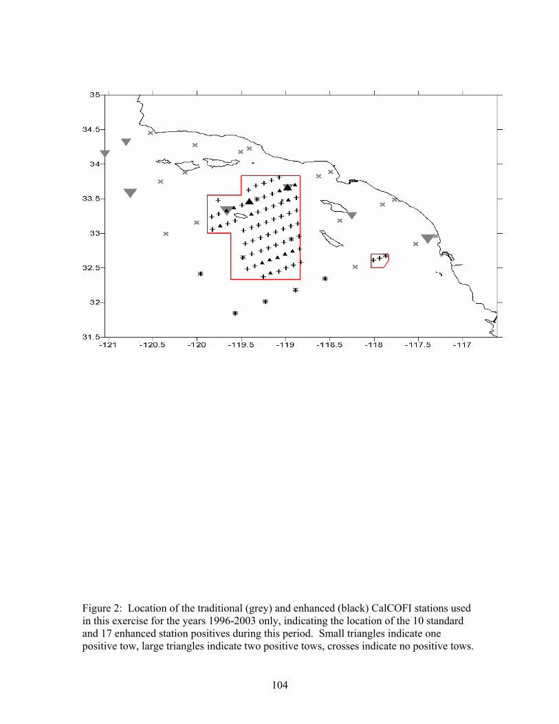
104

Figure 2: Location of the traditional (grey) and enhanced (black) CalCOFI stations used in this exercise for the years 1996-2003 only, indicating the location of the 10 standard and 17 enhanced station positives during this period. Small triangles indicate one positive tow, large triangles indicate two positive tows, crosses indicate no positive tows.

105

Figure 3: Number and percentage of tows positive for cowcod larvae in five year intervals since 1951, including the percentage of positive tows in the most recent (2001-2003) period when enhanced cowcod data are used.

CalCOFI tows positive for cowcod (S. levis ) larvae, 1951-2003

0

10

20

30

40

50

1951-1955

1956-1960

1961-1965

1966-1970

1971-1975

1976-1980

1981-1985

1986-1990

1991-1995

1996-2000

2001-2003

num

ber p

ositi

ves

0.00

0.02

0.04

0.06

0.08

0.10

0.12

% p

ositi

ve

outside pos inside pos % pos outside% pos inside enhanced enhanced

106

Figure 4: The distribution of the point estimates for the expansion factor, based on the variances estimated by the delta method

0

0.1

0.2

0.3

0.4

0.5

0.6

0 0.5 1 1.5 2 2.5 3 3.5 4 4.5 5 5.5 6 6.5

binomial model, all yearsbinomial- all years- excluding enhancedDelta-GLM, all yearsbinomial model (1996-2003 only) binomial model (1996-2003 only) - excluding enhanced

107

Appendix VI. Numbers at age for model h=0.5. Numbers are given every 10 years except in the most recent period.

Year 1914 1920 1930 1940 1950 1960 1970 1975 1980 1985 1990 1995 2000 2001 2002 2003 2004 2005age0 59.5551 59.1434 58.837 58.6666 58.3483 56.0677 52.2639 47.628 39.6995 31.166 17.3169 19.5965 23.4886 24.3218 25.2408 26.0972 26.9011 27.65811 56.368 56.0097 55.717 55.5269 55.2715 53.3293 49.7968 46.5461 39.2238 32.4271 16.1381 18.4719 21.4188 22.2316 23.0202 23.8901 24.7007 25.46152 53.3515 53.0662 52.7662 52.5578 52.3522 50.7645 47.634 45.0602 38.137 31.3412 17.4866 16.7916 19.287 20.2726 21.0419 21.7883 22.6116 23.37883 50.4964 50.275 49.9723 49.7528 49.5945 48.3294 45.7754 43.3911 37.3688 31.395 18.5848 15.7148 17.3755 18.2549 19.1877 19.9158 20.6223 21.40154 47.7941 47.6108 47.3354 47.1 46.9979 46.0429 43.8125 41.4489 37.0373 30.3555 21.7166 14.3232 16.2083 16.4457 17.278 18.1609 18.85 19.51875 45.2364 45.2364 44.8242 44.5906 44.5536 43.8292 41.6757 39.6982 36.1769 30.1546 23.6728 13.1535 14.885 15.3409 15.5656 16.3533 17.189 17.84136 42.8156 42.8156 42.4419 42.2137 42.1907 41.6446 39.5849 37.8243 35.3551 29.7933 24.6307 12.2581 14.0307 14.0884 14.5199 14.7326 15.4782 16.26927 40.5243 40.5243 40.189 39.965 39.9298 39.5065 37.6218 36.1814 34.2265 28.9677 23.8059 13.2823 12.7544 13.2799 13.3345 13.7429 13.9442 14.64998 38.3556 38.3556 38.0517 37.8415 37.7816 37.4757 35.7578 34.7694 32.9582 28.3835 23.846 14.1162 11.9365 12.0719 12.5692 12.6209 13.0074 13.19799 36.303 36.3029 36.0309 35.8406 35.7599 35.5228 33.9889 33.2745 31.4777 28.1226 23.049 16.491 10.8791 11.2975 11.4258 11.8965 11.9455 12.311310 34.3603 34.3592 34.1216 33.9453 33.8459 33.6561 32.3359 31.6206 30.1058 27.3963 22.831 17.9401 9.98805 10.2951 10.6927 10.8142 11.2597 11.306111 32.5215 32.5161 32.309 32.1426 32.0275 31.8499 30.7062 29.8995 28.5001 26.4564 22.2284 18.4934 9.29686 9.44572 9.74342 10.1198 10.2348 10.656612 30.7811 30.7644 30.5996 30.4338 30.2979 30.0901 29.0988 28.107 26.8313 24.9034 20.6893 17.4663 10.0417 8.78066 8.9385 9.22037 9.57668 9.6856713 29.1339 29.0985 28.9716 28.8114 28.6537 28.3795 27.4779 26.2668 25.1278 22.9826 18.6235 16.8375 10.6025 9.47041 8.30805 8.45765 8.72457 9.0619114 27.5748 27.5171 27.4125 27.2764 27.0903 26.7329 25.8806 24.4702 23.2448 20.8382 16.2916 15.4484 12.2245 9.98718 8.95968 7.86032 8.00212 8.2548915 26.0991 26.0203 26.018 25.8115 25.6043 25.16 24.3107 22.7903 21.2253 18.8128 13.6158 14.3733 13.0059 11.5036 9.44773 8.47613 7.4364 7.5708116 24.7024 24.6063 24.5967 24.4196 24.1929 23.635 22.7806 21.1906 19.2554 16.7823 11.177 13.0914 13.0408 12.2279 10.8813 8.93717 8.01845 7.0351417 23.3805 23.2705 23.2511 23.1013 22.8588 22.1815 21.3089 19.6907 17.4182 14.9347 9.02721 11.4419 11.996 12.2498 11.5655 10.2926 8.45403 7.5853118 22.1293 22.0076 21.9771 21.8486 21.603 20.8106 19.9207 18.2598 15.7214 13.2783 7.23749 9.72911 11.306 11.2585 11.5853 10.9389 9.7355 7.9968719 20.945 20.8129 20.7708 20.6618 20.423 19.5288 18.5933 16.9025 14.1725 11.6879 5.73063 8.06618 10.1662 10.6015 10.6469 10.9569 10.3462 9.2084720 19.8242 19.6826 19.6283 19.5383 19.3069 18.3243 17.3306 15.6066 12.7782 10.1584 4.51254 6.39352 9.27731 9.52411 10.0248 10.0686 10.3624 9.7854621 18.7633 18.613 18.5456 18.4718 18.2469 17.1912 16.1278 14.3741 11.4996 8.76701 3.49644 4.97512 8.28793 8.68352 9.00529 9.47955 9.52171 9.8002322 17.7592 17.6011 17.5193 17.4686 17.2444 16.1267 14.9892 13.2138 10.339 7.53909 2.68882 3.80601 7.10331 7.75048 8.20982 8.51487 8.96405 9.0045623 16.8088 16.6438 16.5462 16.5165 16.2953 15.1271 13.9164 12.1394 9.2741 6.4648 2.05517 2.88823 5.92156 6.63673 7.32709 7.76216 8.05129 8.4766524 15.9093 15.7381 15.6247 15.6073 15.3994 14.1868 12.9095 11.1345 8.30261 5.53428 1.5474 2.16341 4.81237 5.52769 6.27368 6.92705 7.33906 7.6130525 15.0579 14.8814 14.7541 14.7944 14.5464 13.3016 11.967 10.1994 7.41395 4.73715 1.14499 1.61103 3.73868 4.48833 5.22489 5.93072 6.54904 6.9391726 14.2521 14.071 13.9328 13.9685 13.7376 12.4685 11.0732 9.32905 6.60448 4.04699 0.83754 1.18031 2.85143 3.48393 4.24214 4.93892 5.60672 6.1918227 13.4894 13.3045 13.1582 13.1875 12.9732 11.688 10.2375 8.5235 5.87349 3.45436 0.60789 0.858308 2.13815 2.65488 3.29258 4.00968 4.6688 5.3005928 12.7675 12.5796 12.4269 12.4492 12.2484 10.9597 9.46282 7.78114 5.22163 2.94245 0.43824 0.620499 1.59061 1.98911 2.50888 3.11194 3.79014 4.4136329 12.0842 11.894 11.7363 11.7511 11.5633 10.2812 8.75021 7.09934 4.63657 2.5025 0.31424 0.442062 1.16819 1.47853 1.87958 2.37107 2.94138 3.5827930 11.4375 11.2457 11.084 11.091 10.9161 9.64559 8.09216 6.47475 4.11366 2.12402 0.22451 0.30967 0.85316 1.08503 1.39702 1.77623 2.24099 2.780331 10.8255 10.6325 10.4679 10.4664 10.3032 9.04813 7.48417 5.89645 3.64635 1.79961 0.15956 0.214592 0.6132 0.791809 1.02514 1.32012 1.67868 2.1181632 10.2461 10.0527 9.88597 9.87531 9.72789 8.4887 6.92318 5.36719 3.23053 1.52332 0.11294 0.14767 0.4376 0.568679 0.74805 0.968646 1.24755 1.5865933 9.69783 9.50445 9.33641 9.31581 9.18322 7.96435 6.40577 4.88633 2.8617 1.2901 0.07954 0.101022 0.31057 0.405531 0.53722 0.706791 0.91535 1.1790534 9.17885 8.98603 8.81746 8.78685 8.66437 7.47424 5.92783 4.45211 2.53532 1.09229 0.05577 0.068807 0.2173 0.287608 0.38307 0.507556 0.66787 0.86504735 8.68764 8.49582 8.32744 8.28789 8.20084 7.01258 5.48607 4.05865 2.24697 0.92496 0.03891 0.046745 0.14956 0.201098 0.27166 0.361901 0.47958 0.63113536 8.22273 8.03232 7.86476 7.81799 7.7318 6.57927 5.07782 3.70185 1.99003 0.783364 0.02703 0.031626 0.10188 0.13832 0.18994 0.256636 0.34194 0.45318337 7.78269 7.59406 7.42791 7.37546 7.28931 6.17368 4.70186 3.37855 1.76304 0.66385 0.01871 0.021336 0.06894 0.09416 0.13064 0.179422 0.24247 0.32310238 7.3662 7.17969 7.01547 6.95839 6.87187 5.79295 4.35672 3.0856 1.56349 0.563129 0.01292 0.014339 0.04641 0.063683 0.08892 0.123398 0.16951 0.22910239 6.972 6.78791 6.62608 6.56512 6.47805 5.43641 4.04023 2.8197 1.3888 0.478318 0.00889 0.009606 0.03111 0.04284 0.06014 0.083993 0.11657 0.16015840 6.59889 6.41749 6.25845 6.19423 6.10639 5.1027 3.74855 2.5781 1.23531 0.406914 0.00611 0.006413 0.02082 0.028706 0.04045 0.056801 0.07935 0.1101441 6.24575 6.06728 5.91137 5.84445 5.75551 4.78958 3.47884 2.35853 1.10027 0.346354 0.00418 0.004267 0.01388 0.019197 0.02711 0.038207 0.05366 0.07496342 5.91151 5.73616 5.58368 5.51458 5.42411 4.49808 3.23019 2.15949 0.98143 0.295263 0.00286 0.002833 0.00923 0.012791 0.01813 0.0256 0.03609 0.05069143 5.59516 5.42311 5.27431 5.20351 5.11105 4.2245 3.00066 1.97946 0.87676 0.252274 0.00195 0.001879 0.00612 0.008503 0.01208 0.017118 0.02418 0.03409444 5.29573 5.12713 4.98223 4.91018 4.81563 3.96622 2.7892 1.81671 0.78435 0.216163 0.00133 0.001244 0.00405 0.005634 0.00803 0.011405 0.01617 0.02284245 5.01233 4.84731 4.70645 4.63359 4.53747 3.73633 2.59299 1.66885 0.70263 0.185705 0.0009 0.000823 0.00267 0.003723 0.00532 0.007581 0.01077 0.01527346 4.7441 4.58276 4.44607 4.37277 4.27596 3.50669 2.41141 1.53406 0.63029 0.15995 0.00061 0.000544 0.00175 0.002453 0.00351 0.005023 0.00716 0.01017547 4.49022 4.33264 4.20022 4.12684 4.03008 3.29167 2.24371 1.41144 0.56631 0.138138 0.00041 0.000359 0.00115 0.001612 0.00232 0.003319 0.00474 0.00676348 4.24993 4.09618 3.96807 3.89494 3.79873 3.09029 2.08836 1.29972 0.5098 0.119626 0.00028 0.000236 0.00075 0.001057 0.00152 0.002186 0.00313 0.00448149 4.02249 3.87262 3.74887 3.67626 3.58092 2.90162 1.9447 1.19805 0.45984 0.103863 0.00019 0.000156 0.00049 0.000693 0.001 0.001436 0.00206 0.0029650 3.80723 3.66126 3.54188 3.47004 3.37581 2.72477 1.81184 1.10489 0.41546 0.090404 0.00012 0.000103 0.00032 0.000454 0.00065 0.000942 0.00136 0.0019551 3.60349 3.46144 3.34641 3.27557 3.18265 2.55889 1.68865 1.01969 0.37588 0.078887 8.3E-05 6.73E-05 0.00021 0.000297 0.00043 0.000618 0.00089 0.00128152 3.41065 3.27253 3.16181 3.09216 3.00074 2.4032 1.57518 0.94187 0.34062 0.069027 5.5E-05 4.41E-05 0.00014 0.000194 0.00028 0.000404 0.00058 0.0008453 3.22813 3.09393 2.98748 2.91919 2.82943 2.25702 1.46985 0.87057 0.30913 0.06058 3.6E-05 2.89E-05 9E-05 0.000127 0.00018 0.000265 0.00038 0.00055154 3.05537 2.92508 2.82284 2.75604 2.66809 2.11986 1.3715 0.80532 0.28102 0.05333 2.3E-05 1.89E-05 5.9E-05 8.28E-05 0.00012 0.000173 0.00025 0.00036155 2.89187 2.76545 2.66734 2.60215 2.51614 1.99142 1.28443 0.74556 0.25576 0.047073 1.5E-05 1.23E-05 3.8E-05 5.41E-05 7.8E-05 0.000113 0.00016 0.00023656 2.73711 2.61453 2.52046 2.45698 2.37303 1.87127 1.19875 0.69069 0.23307 0.041649 9.6E-06 8.01E-06 2.5E-05 3.53E-05 5.1E-05 7.38E-05 0.00011 0.00015457 2.59063 2.47184 2.38174 2.32003 2.23823 1.75887 1.11925 0.64059 0.21271 0.036946 6E-06 5.19E-06 1.6E-05 2.3E-05 3.3E-05 4.82E-05 7E-05 0.00010158 2.45199 2.33695 2.2507 2.19083 2.11126 1.6536 1.04545 0.59449 0.19436 0.032855 3.7E-06 3.34E-06 1.1E-05 1.5E-05 2.2E-05 3.14E-05 4.5E-05 6.58E-0559 2.32078 2.20942 2.12692 2.06893 1.99165 1.55494 0.976884 0.55183 0.17784 0.029292 2.2E-06 2.13E-06 6.9E-06 9.72E-06 1.4E-05 2.05E-05 3E-05 4.29E-0560 2.19658 2.08885 2.00999 1.9539 1.87897 1.46243 0.91313 0.51425 0.16293 0.026169 1.2E-06 1.34E-06 4.5E-06 6.31E-06 9.2E-06 1.33E-05 1.9E-05 2.8E-0561 2.07903 1.97486 1.89953 1.84536 1.7728 1.37568 0.853794 0.47769 0.14945 0.023429 6.5E-07 8.38E-07 2.9E-06 4.09E-06 6E-06 8.66E-06 1.3E-05 1.83E-0562 1.96777 1.8671 1.79517 1.74293 1.67276 1.2943 0.798517 0.44402 0.13731 0.021023 3.1E-07 5.13E-07 1.9E-06 2.64E-06 3.9E-06 5.62E-06 8.2E-06 1.19E-0563 1.86247 1.76521 1.69658 1.64626 1.57849 1.21795 0.746983 0.41299 0.12629 0.018903 1.3E-07 3.08E-07 1.2E-06 1.7E-06 2.5E-06 3.64E-06 5.3E-06 7.72E-0664 1.7628 1.66889 1.60344 1.55502 1.48965 1.1463 0.698959 0.38435 0.11623 0.017033 3.5E-08 1.79E-07 7.5E-07 1.09E-06 1.6E-06 2.35E-06 3.4E-06 5.01E-0665 1.66846 1.57783 1.51544 1.4689 1.40592 1.07906 0.654269 0.35789 0.10744 0.015379 2.1E-09 9.94E-08 4.7E-07 6.89E-07 1E-06 1.51E-06 2.2E-06 3.25E-0666 1.57917 1.49173 1.43229 1.38761 1.32698 1.01593 0.612718 0.33342 0.09904 0.013912 4.5E-12 5.19E-08 2.9E-07 4.33E-07 6.5E-07 9.67E-07 1.4E-06 2.1E-0667 1.49466 1.41033 1.35373 1.31086 1.25257 0.95665 0.574063 0.31076 0.09139 0.012614 3.6E-12 2.46E-08 1.8E-07 2.68E-07 4.1E-07 6.14E-07 9.1E-07 1.35E-0668 1.41468 1.33338 1.2795 1.23841 1.18242 0.90098 0.53806 0.28975 0.08441 0.011457 3.1E-12 9.8E-09 1.1E-07 1.64E-07 2.5E-07 3.85E-07 5.8E-07 8.62E-0769 1.33897 1.26063 1.20935 1.17001 1.11627 0.84869 0.504495 0.27028 0.07804 0.010419 2.6E-12 2.71E-09 6.2E-08 9.76E-08 1.5E-07 2.39E-07 3.6E-07 5.47E-0770 1.26732 1.19184 1.14307 1.10542 1.05389 0.79955 0.473182 0.25226 0.07222 0.009522 2.3E-12 1.61E-10 3.4E-08 5.64E-08 9.2E-08 1.46E-07 2.3E-07 3.44E-0771 1.1995 1.12681 1.08044 1.04443 0.99506 0.75338 0.443954 0.23558 0.06688 0.008683 2E-12 3.36E-13 1.8E-08 3.13E-08 5.3E-08 8.69E-08 1.4E-07 2.13E-0772 1.13531 1.06533 1.02125 0.98684 0.93957 0.70997 0.416663 0.22013 0.06198 0.00793 1.7E-12 2.68E-13 8.4E-09 1.63E-08 3E-08 5.03E-08 8.2E-08 1.3E-0773 1.07455 1.00721 0.96531 0.93245 0.88723 0.66917 0.391168 0.20581 0.05749 0.007254 1.5E-12 2.26E-13 3.3E-09 7.67E-09 1.5E-08 2.78E-08 4.7E-08 7.75E-0874 1.01705 0.95226 0.91246 0.88109 0.83785 0.63079 0.367342 0.19252 0.05335 0.006645 1.3E-12 1.92E-13 9.2E-10 3.05E-09 7.2E-09 1.45E-08 2.6E-08 4.48E-0875 0.962618 0.9003 0.8625 0.83258 0.79126 0.5947 0.345066 0.18016 0.04956 0.006095 1.2E-12 1.65E-13 5.4E-11 8.42E-10 2.9E-09 6.83E-09 1.4E-08 2.48E-0876 0.911104 0.85118 0.81529 0.78676 0.74731 0.56074 0.324233 0.16867 0.04607 0.005598 1E-12 1.42E-13 1.1E-13 4.97E-11 7.9E-10 2.72E-09 6.4E-09 1.29E-0877 0.862346 0.80474 0.77067 0.74348 0.70583 0.52879 0.30474 0.15798 0.04286 0.005147 9.1E-13 1.22E-13 9E-14 1.04E-13 4.7E-11 7.5E-10 2.6E-09 6.09E-0978 0.816198 0.76084 0.7285 0.7026 0.66668 0.49872 0.286494 0.14803 0.03991 0.004738 8.1E-13 1.06E-13 7.6E-14 8.23E-14 9.8E-14 4.42E-11 7.1E-10 2.42E-0979 0.772519 0.71933 0.68864 0.66399 0.62974 0.47042 0.269409 0.13876 0.03719 0.004366 7.2E-13 9.24E-14 6.4E-14 6.92E-14 7.8E-14 9.22E-14 4.2E-11 6.68E-1080 13.6631 12.4745 11.9301 11.4766 10.8407 8.01917 4.48708 2.26108 0.58297 0.064047 8.8E-12 9.15E-13 5.1E-13 5.26E-13 5.6E-13 6.04E-13 6.6E-13 4E-11