E C O L O G I C A L I N F O R M A T I C S 1 ( 2 0 0 6 ) 2 4 7 – 2 5 7

ava i l ab l e a t www.sc i enced i rec t . com

www.e l sev i e r. com/ loca te /eco l i n f

Application of a self-organizing map to select representativespecies in multivariate analysis: A case study determiningdiatom distribution patterns across France

Young-Seuk Parka,b,⁎, Juliette Tisonb, Sovan Lekc, Jean-Luc Giraudeld, Michel Costeb,François Delmasb

aDepartment of Biology, Kyung Hee University, Hoegi-dong, Dongdaemun-gu, Seoul 130-701, KoreabU.R. REQUE, Cemagref Bordeaux, 50 av. de Verdun, 33612 Cestas, FrancecLADYBIO, CNRS-Université Paul Sabatier, 118 Route de Narbonne, 31062 Toulouse cedex, FrancedEPCA- LPTC, UMR 5472 CNRS-Université Bordeaux 1, 39 rue Paul Mazy, 24019 Périgueux Cedex, France

A R T I C L E I N F O

⁎ Corresponding author. Department of Biolog0946; fax: +82 2 961 0244.

E-mail address: parkys@khu.ac.kr (Y.-S. Pa

1574-9541/$ - see front matter © 2006 Elsevidoi:10.1016/j.ecoinf.2006.03.005

A B S T R A C T

Article history:Received 9 August 2005Received in revised form1 March 2006Accepted 15 March 2006

Ecological communities consist of a large number of species. Most species are rare or havelow abundance, and only a few are abundant and/or frequent. In quantitative communityanalysis, abundant species are commonly used to interpret patterns of habitat disturbanceor ecosystem degradation. Rare species cause many difficulties in quantitative analysis byintroducing noises and bulking datasets, which is worsened by the fact that large datasetssuffer from difficulties of data handling. In this study we propose a method to reduce thesize of large datasets by selecting the most ecologically representative species using a selforganizing map (SOM) and structuring index (SI). As an example, we used diatomcommunity data sampled at 836 sites with 941 species throughout the Frenchhydrosystem. Out of the 941 species, 353 were selected. The selected dataset waseffectively classified according to the similarities of community assemblages in the SOMmap. Compared to the SOM map generated with the original dataset, the communitypattern gave a very similar representation of ecological conditions of the sampling sites,displaying clear gradients of environmental factors between different clusters. Our resultsshowed that this computational technique can be applied to preprocessing data inmultivariate analysis. It could be useful for ecosystem assessment and management,helping to reduce both the list of species for identification and the size of datasets to beprocessed for diagnosing the ecological status of water courses.

© 2006 Elsevier B.V. All rights reserved.

Keywords:Dimension reductionRepresentative speciesSelf-organizing mapMultivariate analysis

1. Introduction

Biological communities are commonly used as indicators ofecosystem quality. Community structures are determined bymany environmental factors in different spatial and temporalscales (Stevenson, 1997; Snyder et al., 2002). Community dataare composed of a large number of species collected at many

y, Kyung Hee University,

rk).

er B.V. All rights reserved

sampling sites at different times. A commonly observedphenomenon in field surveys is that the vast majority ofspecies are represented by low abundance while only a fewspecies are abundant. Preston's canonical log-normal distri-bution is the most widely accepted formalization of therelative commonness and rarity of species (Preston, 1962;Brown, 1981).

Hoegi-dong, Dongdaemun-gu, Seoul 130-701, Korea. Tel.: +82 2 961

.

248 E C O L O G I C A L I N F O R M A T I C S 1 ( 2 0 0 6 ) 2 4 7 – 2 5 7

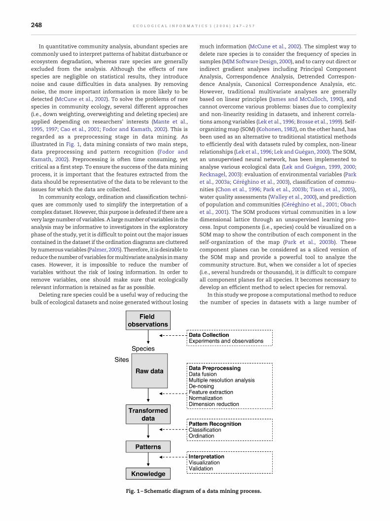
In quantitative community analysis, abundant species arecommonly used to interpret patterns of habitat disturbance orecosystem degradation, whereas rare species are generallyexcluded from the analysis. Although the effects of rarespecies are negligible on statistical results, they introducenoise and cause difficulties in data analyses. By removingnoise, the more important information is more likely to bedetected (McCune et al., 2002). To solve the problems of rarespecies in community ecology, several different approaches(i.e., down weighting, overweighting and deleting species) areapplied depending on researchers' interests (Mante et al.,1995, 1997; Cao et al., 2001; Fodor and Kamath, 2002). This isregarded as a preprocessing stage in data mining. Asillustrated in Fig. 1, data mining consists of two main steps,data preprocessing and pattern recognition (Fodor andKamath, 2002). Preprocessing is often time consuming, yetcritical as a first step. To ensure the success of the dataminingprocess, it is important that the features extracted from thedata should be representative of the data to be relevant to theissues for which the data are collected.

In community ecology, ordination and classification techni-ques are commonly used to simplify the interpretation of acomplex dataset. However, this purpose is defeated if there are avery largenumberof variables.A largenumberof variables in theanalysis may be informative to investigators in the exploratoryphase of the study, yet it is difficult to point out themajor issuescontained in the dataset if the ordination diagrams are clutteredbynumerousvariables (Palmer, 2005).Therefore, it isdesirable toreducethenumberofvariables formultivariateanalysis inmanycases. However, it is impossible to reduce the number ofvariables without the risk of losing information. In order toremove variables, one should make sure that ecologicallyrelevant information is retained as far as possible.

Deleting rare species could be a useful way of reducing thebulk of ecological datasets and noise generated without losing

Fig. 1 –Schematic diagram o

much information (McCune et al., 2002). The simplest way todelete rare species is to consider the frequency of species insamples (MJM Software Design, 2000), and to carry out direct orindirect gradient analyses including Principal ComponentAnalysis, Correspondence Analysis, Detrended Correspon-dence Analysis, Canonical Correspondence Analysis, etc.However, traditional multivariate analyses are generallybased on linear principles (James and McCulloch, 1990), andcannot overcome various problems: biases due to complexityand non-linearity residing in datasets, and inherent correla-tions among variables (Lek et al., 1996; Brosse et al., 1999). Self-organizingmap (SOM) (Kohonen, 1982), on the other hand, hasbeen used as an alternative to traditional statistical methodsto efficiently deal with datasets ruled by complex, non-linearrelationships (Lek et al., 1996; Lek and Guégan, 2000). The SOM,an unsupervised neural network, has been implemented toanalyse various ecological data (Lek and Guégan, 1999, 2000;Recknagel, 2003): evaluation of environmental variables (Parket al., 2003a; Céréghino et al., 2003), classification of commu-nities (Chon et al., 1996; Park et al., 2003b; Tison et al., 2005),water quality assessments (Walley et al., 2000), and predictionof population and communities (Céréghino et al., 2001; Obachet al., 2001). The SOM produces virtual communities in a lowdimensional lattice through an unsupervised learning pro-cess. Input components (i.e., species) could be visualized on aSOM map to show the contribution of each component in theself-organization of the map (Park et al., 2003b). Thesecomponent planes can be considered as a sliced version ofthe SOM map and provide a powerful tool to analyze thecommunity structure. But, when we consider a lot of species(i.e., several hundreds or thousands), it is difficult to compareall component planes for all species. It becomes necessary todevelop an efficient method to select species for removal.

In this studywe propose a computationalmethod to reducethe number of species in datasets with a large number of

f a data mining process.

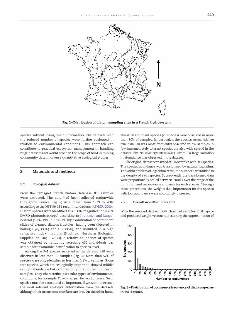
Fig. 2 –Distribution of diatom sampling sites in a French hydrosystem.

249E C O L O G I C A L I N F O R M A T I C S 1 ( 2 0 0 6 ) 2 4 7 – 2 5 7

species without losing much information. The datasets withthe reduced number of species were further evaluated inrelation to environmental conditions. This approach cancontribute to practical ecosystem management in handlinghuge datasets and would broaden the scope of SOM in miningcommunity data in diverse quantitative ecological studies.

2. Materials and methods

Fig. 3 –Distribution of occurrence frequency of diatom speciesin the dataset.

2.1. Ecological dataset

From the Cemagref French Diatom Database, 836 sampleswere extracted. The data had been collected nationwidethroughout France (Fig. 2) in summer from 1979 to 2002according to the NFT 90-354 recommendations (AFNOR, 2000).Diatom species were identified at a 1000× magnification (LeitzDMRD photomicroscope) according to Krammer and Lange-Bertalot (1986, 1988, 1991a, 1991b): examination of permanentslides of cleaned diatom frustules, having been digested inboiling H2O2 (30%) and HCl (35%), and mounted in a highrefractive index medium (Naphrax, Northern BiologicalSupplies Ltd, UK; RI=1.74). A relative abundance of specieswas obtained by randomly selecting 400 individuals persample for taxonomic identification to species level.

Among the 941 species recorded in the dataset, 490 wereobserved in less than 10 samples (Fig. 3). More than 52% ofspecies were only identified in less than 1.2% of samples. Somerare species, which are ecologically important, showed middleor high abundance but occurred only in a limited number ofsamples. They characterize particular types of environmentalconditions, for example Eunotia exigua for acidic rivers. Suchspecies must be considered as important, if we want to extractthe most relevant ecological information from the datasetsalthough their occurrence numbers are low. On the other hand,

about 3% abundant species (25 species) were observed in morethan 50% of samples. In particular, the species Achnanthidiumminutissimum was most frequently observed in 737 samples. Afew intermediately tolerant species are also wide spread in thedataset, like Navicula cryptotenelloides. Overall, a large variationin abundance was observed in the dataset.

Theoriginaldatasetconsistedof836sampleswith941species.The species abundance was transformed by natural logarithm.Toavoidaproblemof logarithmzeros, thenumber1wasadded tothe density of each species. Subsequently the transformed datawere proportionally scaled between 0 and 1 over the range of theminimum and maximum abundance for each species. Throughthese procedures, the weights (i.e., importance) for the specieswith low abundance were accordingly increased.

2.2. Overall modelling procedure

With the rescaled dataset, SOM classified samples in 2D spaceand produced weight vectors representing the approximation of

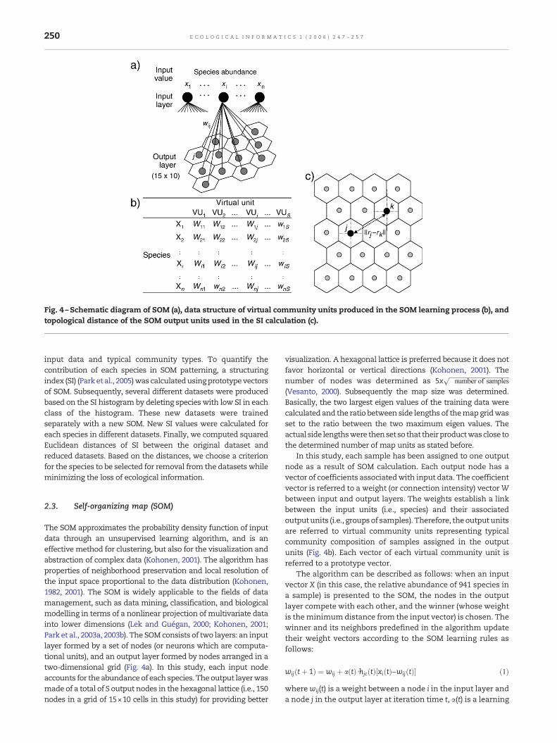
Fig. 4 –Schematic diagram of SOM (a), data structure of virtual community units produced in the SOM learning process (b), andtopological distance of the SOM output units used in the SI calculation (c).

250 E C O L O G I C A L I N F O R M A T I C S 1 ( 2 0 0 6 ) 2 4 7 – 2 5 7

input data and typical community types. To quantify thecontribution of each species in SOM patterning, a structuringindex (SI) (Park et al., 2005)was calculatedusingprototypevectorsof SOM. Subsequently, several different datasets were producedbased on the SI histogram by deleting species with low SI in eachclass of the histogram. These new datasets were trainedseparately with a new SOM. New SI values were calculated foreach species in different datasets. Finally, we computed squaredEuclidean distances of SI between the original dataset andreduced datasets. Based on the distances, we choose a criterionfor the species to be selected for removal from the datasets whileminimizing the loss of ecological information.

2.3. Self-organizing map (SOM)

The SOM approximates the probability density function of inputdata through an unsupervised learning algorithm, and is aneffectivemethod for clustering, but also for the visualization andabstraction of complex data (Kohonen, 2001). The algorithm hasproperties of neighborhood preservation and local resolution ofthe input space proportional to the data distribution (Kohonen,1982, 2001). The SOM is widely applicable to the fields of datamanagement, such as data mining, classification, and biologicalmodelling in terms of a nonlinear projection of multivariate datainto lower dimensions (Lek and Guégan, 2000; Kohonen, 2001;Park et al., 2003a, 2003b). The SOMconsists of two layers: an inputlayer formed by a set of nodes (or neurons which are computa-tional units), and an output layer formed by nodes arranged in atwo-dimensional grid (Fig. 4a). In this study, each input nodeaccounts for the abundance of each species. Theoutput layerwasmade of a total of S output nodes in the hexagonal lattice (i.e., 150nodes in a grid of 15×10 cells in this study) for providing better

visualization. A hexagonal lattice is preferred because it does notfavor horizontal or vertical directions (Kohonen, 2001). Thenumber of nodes was determined as 5x

ffiffiffiffiffiffiffiffiffiffiffiffiffiffiffiffiffiffiffiffiffiffiffiffiffiffiffiffiffiffiffiffiffiffiffiffiffiffiffinumber of samples

p

(Vesanto, 2000). Subsequently the map size was determined.Basically, the two largest eigen values of the training data werecalculated and the ratio between side lengths of themapgridwasset to the ratio between the two maximum eigen values. Theactual side lengthswere thensetso that theirproductwasclose tothe determined number of map units as stated before.

In this study, each sample has been assigned to one outputnode as a result of SOM calculation. Each output node has avector of coefficients associatedwith input data. The coefficientvector is referred to a weight (or connection intensity) vectorWbetween input and output layers. The weights establish a linkbetween the input units (i.e., species) and their associatedoutputunits (i.e., groupsof samples). Therefore, theoutputunitsare referred to virtual community units representing typicalcommunity composition of samples assigned in the outputunits (Fig. 4b). Each vector of each virtual community unit isreferred to a prototype vector.

The algorithm can be described as follows: when an inputvector X (in this case, the relative abundance of 941 species ina sample) is presented to the SOM, the nodes in the outputlayer compete with each other, and the winner (whose weightis theminimumdistance from the input vector) is chosen. Thewinner and its neighbors predefined in the algorithm updatetheir weight vectors according to the SOM learning rules asfollows:

wijðtþ 1Þ ¼ wij þ aðtÞdhjcðtÞ½xiðtÞ−wijðtÞ� ð1Þ

wherewij(t) is a weight between a node i in the input layer anda node j in the output layer at iteration time t, α(t) is a learning

251E C O L O G I C A L I N F O R M A T I C S 1 ( 2 0 0 6 ) 2 4 7 – 2 5 7

rate factor which is a decreasing function of the iteration timet, and hjc(t) is a neighborhood function (a smoothing kerneldefined over the lattice points) that defines the size ofneighborhood of the winning node (c) to be updated duringthe learning process. This learning process is continued until astopping criterion is met, usually, when weight vectorsstabilize or when a number of iterations are completed. Thislearning process results in the preservation of the connectionintensities in the weight vectors.

2.4. Structuring index (SI)

The SI was originally developed to define species showing thestrongest influence on the organization of the SOMmap (Park etal., 2005). Tison et al. (2004, 2005) used theSI to evaluate relevantdiatomspecies in the classification of diatomcommunities. TheSI is the value indicating the relative importance of each speciesin determining the distribution patterns of the samples in theSOM. Therefore, the set of species showing high SI can beconsidered as the indicator species.

The SI is calculated from the sumof the ratios of the distancebetweentheweights (i.e., connection intensities) ofall species inthe SOM and the topological distance between two SOM units

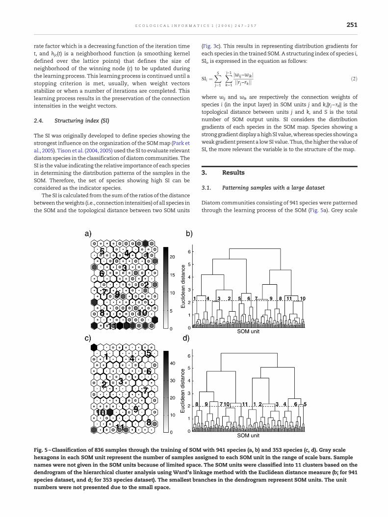
Fig. 5 –Classification of 836 samples through the training of SOMhexagons in each SOM unit represent the number of samples asnames were not given in the SOM units because of limited spacedendrogram of the hierarchical cluster analysis using Ward's linspecies dataset, and d; for 353 species dataset). The smallest branumbers were not presented due to the small space.

(Fig. 3c). This results in representing distribution gradients foreach species in the trainedSOM. A structuring index of species i,SIi, is expressed in the equation as follows:

SIi ¼XS

j¼1

Xj−1

k¼1

jwij−wikjjjrj−rkjj

ð2Þ

where wij and wik are respectively the connection weights ofspecies i (in the input layer) in SOM units j and k,||rj−rk|| is thetopological distance between units j and k, and S is the totalnumber of SOM output units. SI considers the distributiongradients of each species in the SOM map. Species showing astronggradientdisplayahighSIvalue,whereasspeciesshowingaweakgradientpresenta lowSIvalue.Thus, thehigher thevalueofSI, the more relevant the variable is to the structure of the map.

3. Results

3.1. Patterning samples with a large dataset

Diatom communities consisting of 941 species were patternedthrough the learning process of the SOM (Fig. 5a). Grey scale

with 941 species (a, b) and 353 species (c, d). Gray scalesigned to each SOM unit in the range of scale bars. Sample. The SOM units were classified into 11 clusters based on thekage method with the Euclidean distance measure (b; for 941nches in the dendrogram represent SOM units. The unit

252 E C O L O G I C A L I N F O R M A T I C S 1 ( 2 0 0 6 ) 2 4 7 – 2 5 7

hexagons represent the number of samples assigned in eachSOM unit in the range of 2 (small white)–22 (large black). TheSOM units were further grouped into 11 clusters based on thedendrogram of a hierarchical cluster analysis (Fig. 5b).

The SOMweight vectorswere used for the classification of theunits. Overall diatom communities were well organized in theSOM map according to similarities of their species composition.

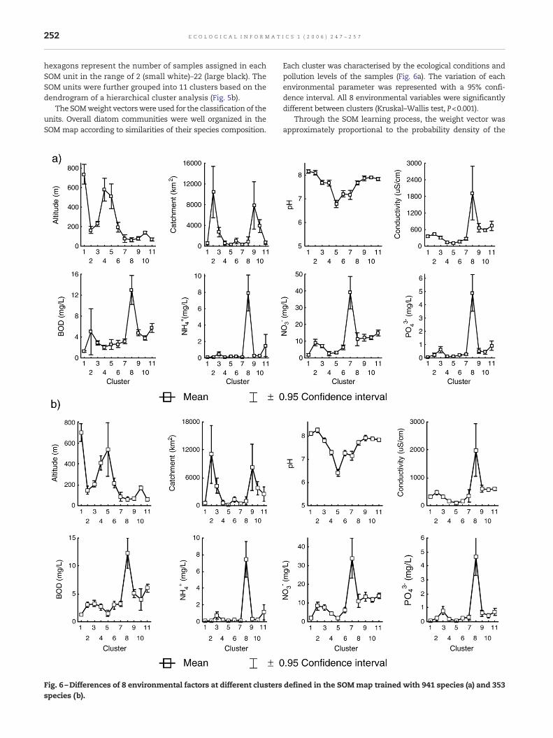
Fig. 6 –Differences of 8 environmental factors at different clustersspecies (b).

Each cluster was characterised by the ecological conditions andpollution levels of the samples (Fig. 6a). The variation of eachenvironmental parameter was represented with a 95% confi-dence interval. All 8 environmental variables were significantlydifferent between clusters (Kruskal–Wallis test, P<0.001).

Through the SOM learning process, the weight vector wasapproximately proportional to the probability density of the

defined in the SOMmap trained with 941 species (a) and 353

253E C O L O G I C A L I N F O R M A T I C S 1 ( 2 0 0 6 ) 2 4 7 – 2 5 7

data. Therefore, each species distribution in the SOM outputunits can provide their importance in the community structure.Fig. 7a shows examples of distribution gradients of species inthe SOM map trained with 941 species. Dark represents a highvalueof speciesdensity in their givenscalebar,whereaswhite isa low value. The values indicate estimated abundances ofspecies in log scale which were denormalized from weightvectors based on the minimum and maximum values of eachspecies defined in the input dataset. All species showed thestrong gradient in different ways, although some speciesshowed bi- or multi-modal distribution patterns. While somespecies showed very similar patterns of gradient on the map,their contributions to patterning on the map were different bydisplaying different abundances and SI. For instance, Eunotiabilunaris andAchnanthidium eutrophilumweremainly distributedin the samples assigned to the upper left areas of the SOMmap.

Fig. 7 –Gradient distributions of example species in the SOM mafollowing species acronyms are the SI values for each species. Slearning process in log scale. AAMB, Aulacoseira ambigua, ACOFminutissimum, ADSU; A. subatomus, ASHU; Achnanthes subhuPlanothidium ellipticum, SKPO; S. potamos, SLCO; S. linearis.

However, estimated abundances between two species werestrongly variable, indicating differences of their contributions tocommunitypatterns.ThesamesituationwasobservedbetweenAchnanthidium subatomus and Surirella linearis and between Ske-letonemapotamos andGomphonema entolejum. From these typesofvisualizing component planes, we can evaluate the relativeimportance of each species. For instance, A. subatomus is moreimportant in characterizing samples belonging to the middleupper areas of the SOMmap than S. linearis.

However, evaluation of contributions becomes difficultfrom component planes when the numbers of input variables(i.e., species) are very large as stated before. In this study therelative importance of each species was expressed throughthe SI. The priority of selection for the datasets wasdetermined by the values of the SI (Fig. 8). The SI values ofexample species are given in Fig. 7, while a profile of the SI

p trained with 941 species (a) and 353 species (b). Valuescale bar shows species abundance calculated through SOM; Amphora coffeaeformis, ADEU; A. eutrophilum, ADMI; A.dsonis, EBIL; E. bilunaris, GENT; G. entolejum, PTEL;

Fig. 8 –Number of species at different classes of SI in theoriginal dataset containing 941 species. Based on the SIclasses, 8 different datasets were built by excluding speciesshowing low SI.

Fig. 9 –Similarity distances of species SI between the originaldataset and 8 reduced datasets. In the distance calculations,145 species included in the smallest dataset were used.

254 E C O L O G I C A L I N F O R M A T I C S 1 ( 2 0 0 6 ) 2 4 7 – 2 5 7

values over 941 species is given in different classes in Fig. 8.More than 49% of species showed less than 20 SI values (in thefirst and the second classes from the left on the x axis). Thenumber of species decreased gradually until the 8th class (60–70 SI). The contributions of most species beyond the 8th classwere very low in defining community patterns.

3.2. Selection of relevant species

The next step is to evaluate different datasets where relevantspecies were selected according to values of SI. SOM trainingswere independently repeated with 8 successive datasets asshown in Fig. 8. The SI values were summed for all species ineach dataset. Subsequently the sum of Euclidean distances ofthe SI values between the original dataset and the reduceddatasets were calculated (Fig. 9). Datasets consisting of a smallnumber of abundant species showed high SI values for mostspecies, whereas larger datasets with diverse species coveredspecies with both high and low SI values. As the number ofspecies decreased, the Euclidean distance increased abruptlyaround the number of species approximately equal to 353whereas the distances were gradually decreased as thenumber of species further increased to 941. The profile of thedistances indicates that elimination of species after 353 wouldnot seriously affect the predictive characteristics of theoriginal dataset. Consequently the profile of the distances(Fig. 9) shows a criterion to choose the SI value to select theappropriate number of species while minimizing the loss ofinformation due to removal of extra species. Here, we chosethe 3rd class with 353 species based on the above reasoning.Regression analyses were carried out between SI values of thetotal species (941) and each of the datasets with the reducednumber of species. In the case of the 353 species dataset, theregression determination coefficient was distinctively high(R2=0.991) (Fig. 10) while the coefficients for the datasets witha lower number of species (145 and 220) were substantiallylower. This indicates that the community information ispreserved in a new reduced dataset with 353 species.

3.3. Patterning samples with reduced dataset

To evaluate the dataset with 353 relevant species, 836 sampleswere trained with the SOM (Fig. 5c). The numbers of samplesassigned to each SOM unit are indicated in a grey scale ashexagons ranging from 0 (small white) to 47 (large black). TheSOM units were classified into 11 clusters through a hierarchi-cal cluster analysis based on Ward's linkage method (Fig. 5d).The grouping was essentially the same as those of the originaldataset (Fig. 5a,b). Overall, diatom communities were wellorganized in the SOM map according to similarities of speciescomposition. Each cluster was well characterised by the ecolo-gical and pollution conditions of the sampling sites (Fig. 6b).All 8 environmental variables were significantly different be-tween clusters (Kruskal–Wallis test, P<0.001). Samples inclusters 1–6 (in the upper areas of the SOM map) were mainlycollected from the sites showing higher water quality,whereas the samples in clusters 7–11 (in the bottom areas ofthe SOM map) were observable from disturbed sites. Thedifference of communities (communities in good water qual-ity versus communities under anthropogenic disturbances)was clearly distinguished in two main clusters in the den-drogram of the SOM units (Fig. 5d). The clusters were well inaccordance with those of the original dataset with 941 species(Fig. 5). The characteristics of each cluster are summarized inTable 1.

Fig. 7b shows the abundance patterns of some selectedspecies in the reduced dataset with 353 species. The patternswere similar to the original dataset (Fig. 7a), although theirrelative positions in the SOMmap were changed to somewhatlike mirror images. For example, E. bilunaris showed highvalues in the upper right areas of the SOM map in the originaldataset, but was abundant in the upper left areas in thereduced dataset. A. minutissimum showed high values in theupper right areas in the original dataset, while the abundancewas higher in the upper left areas of the reduced dataset. Theresults in Figs. 6 and 7 indicate that removal of a substantialnumber of species according to the SI did not affect thepreservation of useful information residing in the originaldataset. Species richness between the original dataset and the

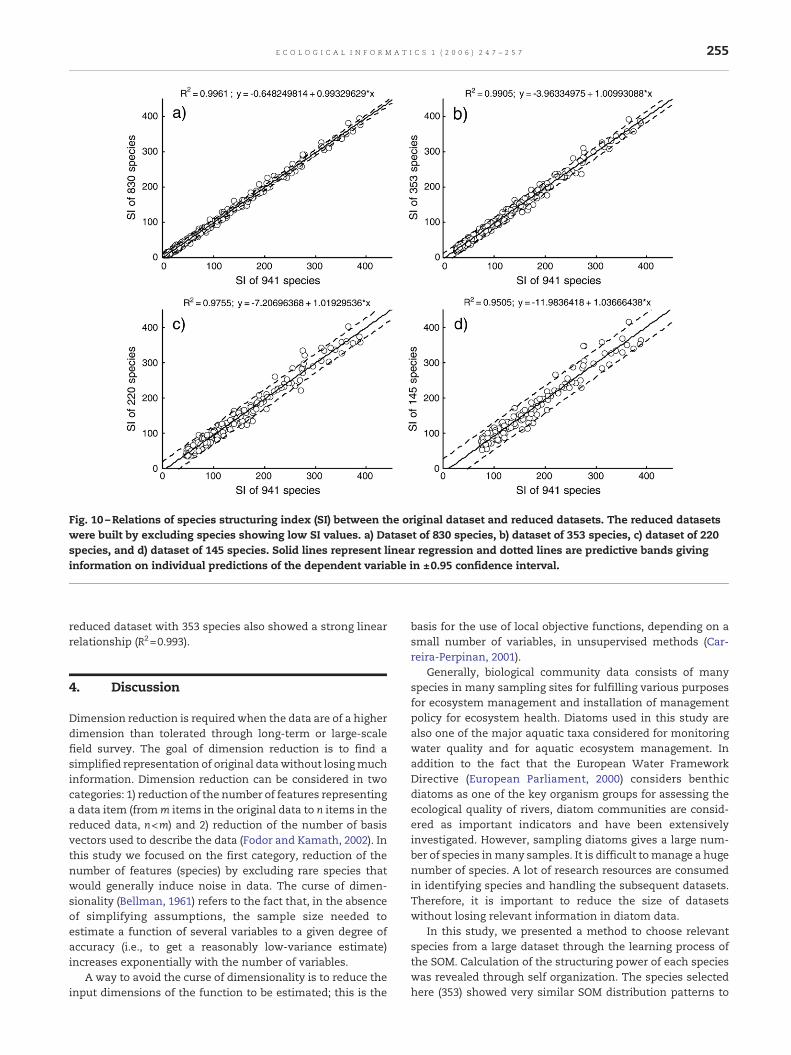
Fig. 10 –Relations of species structuring index (SI) between the original dataset and reduced datasets. The reduced datasetswere built by excluding species showing low SI values. a) Dataset of 830 species, b) dataset of 353 species, c) dataset of 220species, and d) dataset of 145 species. Solid lines represent linear regression and dotted lines are predictive bands givinginformation on individual predictions of the dependent variable in ±0.95 confidence interval.

255E C O L O G I C A L I N F O R M A T I C S 1 ( 2 0 0 6 ) 2 4 7 – 2 5 7

reduced dataset with 353 species also showed a strong linearrelationship (R2=0.993).

4. Discussion

Dimension reduction is required when the data are of a higherdimension than tolerated through long-term or large-scalefield survey. The goal of dimension reduction is to find asimplified representation of original datawithout losingmuchinformation. Dimension reduction can be considered in twocategories: 1) reduction of the number of features representinga data item (fromm items in the original data to n items in thereduced data, n<m) and 2) reduction of the number of basisvectors used to describe the data (Fodor and Kamath, 2002). Inthis study we focused on the first category, reduction of thenumber of features (species) by excluding rare species thatwould generally induce noise in data. The curse of dimen-sionality (Bellman, 1961) refers to the fact that, in the absenceof simplifying assumptions, the sample size needed toestimate a function of several variables to a given degree ofaccuracy (i.e., to get a reasonably low-variance estimate)increases exponentially with the number of variables.

A way to avoid the curse of dimensionality is to reduce theinput dimensions of the function to be estimated; this is the

basis for the use of local objective functions, depending on asmall number of variables, in unsupervised methods (Car-reira-Perpinan, 2001).

Generally, biological community data consists of manyspecies in many sampling sites for fulfilling various purposesfor ecosystem management and installation of managementpolicy for ecosystem health. Diatoms used in this study arealso one of the major aquatic taxa considered for monitoringwater quality and for aquatic ecosystem management. Inaddition to the fact that the European Water FrameworkDirective (European Parliament, 2000) considers benthicdiatoms as one of the key organism groups for assessing theecological quality of rivers, diatom communities are consid-ered as important indicators and have been extensivelyinvestigated. However, sampling diatoms gives a large num-ber of species inmany samples. It is difficult tomanage a hugenumber of species. A lot of research resources are consumedin identifying species and handling the subsequent datasets.Therefore, it is important to reduce the size of datasetswithout losing relevant information in diatom data.

In this study, we presented a method to choose relevantspecies from a large dataset through the learning process ofthe SOM. Calculation of the structuring power of each specieswas revealed through self organization. The species selectedhere (353) showed very similar SOM distribution patterns to

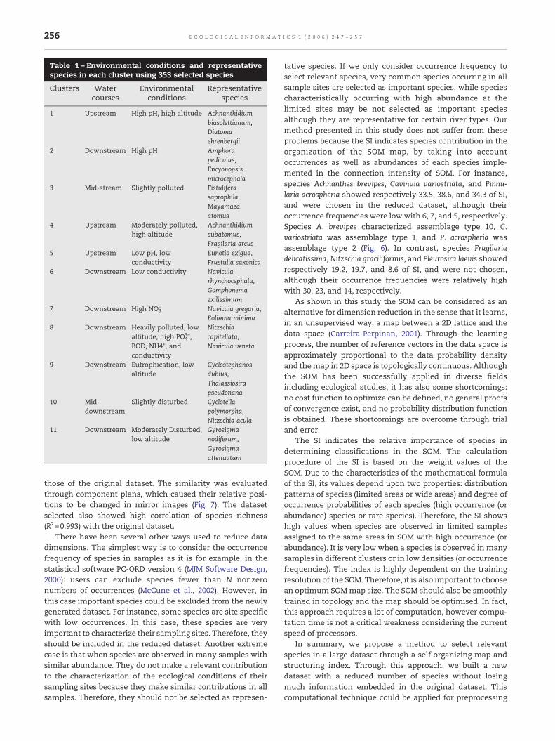
Table 1 – Environmental conditions and representativespecies in each cluster using 353 selected species

Clusters Watercourses

Environmentalconditions

Representativespecies

1 Upstream High pH, high altitude Achnanthidiumbiasolettianum,Diatomaehrenbergii

2 Downstream High pH Amphorapediculus,Encyonopsismicrocephala

3 Mid-stream Slightly polluted Fistuliferasaprophila,Mayamaeaatomus

4 Upstream Moderately polluted,high altitude

Achnanthidiumsubatomus,Fragilaria arcus

5 Upstream Low pH, lowconductivity

Eunotia exigua,Frustulia saxonica

6 Downstream Low conductivity Navicularhynchocephala,Gomphonemaexilissimum

7 Downstream High NO3− Navicula gregaria,

Eolimna minima8 Downstream Heavily polluted, low

altitude, high PO43−,

BOD, NH4+, andconductivity

Nitzschiacapitellata,Navicula veneta

9 Downstream Eutrophication, lowaltitude

Cyclostephanosdubius,Thalassiosirapseudonana

10 Mid-downstream

Slightly disturbed Cyclotellapolymorpha,Nitzschia acula

11 Downstream Moderately Disturbed,low altitude

Gyrosigmanodiferum,Gyrosigmaattenuatum

256 E C O L O G I C A L I N F O R M A T I C S 1 ( 2 0 0 6 ) 2 4 7 – 2 5 7

those of the original dataset. The similarity was evaluatedthrough component plans, which caused their relative posi-tions to be changed in mirror images (Fig. 7). The datasetselected also showed high correlation of species richness(R2=0.993) with the original dataset.

There have been several other ways used to reduce datadimensions. The simplest way is to consider the occurrencefrequency of species in samples as it is for example, in thestatistical software PC-ORD version 4 (MJM Software Design,2000): users can exclude species fewer than N nonzeronumbers of occurrences (McCune et al., 2002). However, inthis case important species could be excluded from the newlygenerated dataset. For instance, some species are site specificwith low occurrences. In this case, these species are veryimportant to characterize their sampling sites. Therefore, theyshould be included in the reduced dataset. Another extremecase is that when species are observed in many samples withsimilar abundance. They do not make a relevant contributionto the characterization of the ecological conditions of theirsampling sites because they make similar contributions in allsamples. Therefore, they should not be selected as represen-

tative species. If we only consider occurrence frequency toselect relevant species, very common species occurring in allsample sites are selected as important species, while speciescharacteristically occurring with high abundance at thelimited sites may be not selected as important speciesalthough they are representative for certain river types. Ourmethod presented in this study does not suffer from theseproblems because the SI indicates species contribution in theorganization of the SOM map, by taking into accountoccurrences as well as abundances of each species imple-mented in the connection intensity of SOM. For instance,species Achnanthes brevipes, Cavinula variostriata, and Pinnu-laria acrospheria showed respectively 33.5, 38.6, and 34.3 of SI,and were chosen in the reduced dataset, although theiroccurrence frequencies were low with 6, 7, and 5, respectively.Species A. brevipes characterized assemblage type 10, C.variostriata was assemblage type 1, and P. acrospheria wasassemblage type 2 (Fig. 6). In contrast, species Fragilariadelicatissima, Nitzschia graciliformis, and Pleurosira laevis showedrespectively 19.2, 19.7, and 8.6 of SI, and were not chosen,although their occurrence frequencies were relatively highwith 30, 23, and 14, respectively.

As shown in this study the SOM can be considered as analternative for dimension reduction in the sense that it learns,in an unsupervised way, a map between a 2D lattice and thedata space (Carreira-Perpinan, 2001). Through the learningprocess, the number of reference vectors in the data space isapproximately proportional to the data probability densityand themap in 2D space is topologically continuous. Althoughthe SOM has been successfully applied in diverse fieldsincluding ecological studies, it has also some shortcomings:no cost function to optimize can be defined, no general proofsof convergence exist, and no probability distribution functionis obtained. These shortcomings are overcome through trialand error.

The SI indicates the relative importance of species indetermining classifications in the SOM. The calculationprocedure of the SI is based on the weight values of theSOM. Due to the characteristics of the mathematical formulaof the SI, its values depend upon two properties: distributionpatterns of species (limited areas or wide areas) and degree ofoccurrence probabilities of each species (high occurrence (orabundance) species or rare species). Therefore, the SI showshigh values when species are observed in limited samplesassigned to the same areas in SOM with high occurrence (orabundance). It is very low when a species is observed in manysamples in different clusters or in low densities (or occurrencefrequencies). The index is highly dependent on the trainingresolution of the SOM. Therefore, it is also important to choosean optimum SOMmap size. The SOM should also be smoothlytrained in topology and the map should be optimised. In fact,this approach requires a lot of computation, however compu-tation time is not a critical weakness considering the currentspeed of processors.

In summary, we propose a method to select relevantspecies in a large dataset through a self organizing map andstructuring index. Through this approach, we built a newdataset with a reduced number of species without losingmuch information embedded in the original dataset. Thiscomputational technique could be applied for preprocessing

257E C O L O G I C A L I N F O R M A T I C S 1 ( 2 0 0 6 ) 2 4 7 – 2 5 7

data in multivariate analyses and could be useful in ecosys-tem management needing to reduce the number of variablesin large datasets. Our work on dimension reduction could bealso helpful for data management and data mining in variousother fields of research.

Acknowledgements

This work was supported by the EU projects Rebecca (contractnumber SSPI-CT-2003-502158) and the Euro-limpacs (contractnumber GOEC-CT-2003-505540).

R E F E R E N C E S

AFNOR, 2000. NFT 90-354: Détermination de l'indice biologiquediatomées (IBD). Agence de l'Eau Artois-Picardie, Douai.

Bellman, R., 1961. Adaptive Control Processes: A Guided Tour.Princeton University Press, New Jersey.

Brosse, S., Guegan, J.F., Tourenq, J.N., Lek, S., 1999. The use ofartificial neural networks to assess fish abundance and spatialoccupancy in the littoral zone of a mesotrophic lake. Ecol.Model. 120, 299–311.

Brown, J.H., 1981. Two decades of homage to Santa Rosalia: towarda general theory of diversity. Am. Zool. 21, 877–888.

Cao, Y., Larsen, D.P., Thorne, RSt-J., 2001. Rare species inmultivariate analysis for bioassessment: some considerations.J. N. Am. Benthol. Soc. 20, 144–153.

Carreira-Perpinan, M.A., 2001. Continuous latent variable modelsfor dimensionality reduction and sequential data reconstruc-tion. PhD thesis, University of Sheffield, Sheffield, UK.

Céréghino, R., Giraudel, J.L., Compin, A., 2001. Spatial analysis ofstream invertebrates distribution in the Adour–Garonnedrainage basin (France), using Kohonen self organizing maps.Ecol. Model. 146, 167–180.

Céréghino, R., Park, Y.-S., Compin, A., Lek, S., 2003. Predicting thespecies richness of aquatic insects in streams using a restrictednumber of environmental variables. J. N. Am. Benthol. Soc. 22,442–456.

Chon, T.-S., Park, Y.-S., Moon, K.H., Cha, E.Y., 1996. Patternizingcommunities by using an artificial neural network. Ecol. Model.90, 69–78.

European Parliament, 2000. Directive 2000/60/EC of the EuropeanParliament and of the Council establishing a framework forcommunity action in the field of water policy. Off. J. L 327, 1–72.

Fodor, I.K., Kamath, C., 2002. Dimension reduction techniques andthe classification of bent double galaxies. Comput. Stat. DataAnal. 41, 91–122.

James, F.C., McCulloch, C.E., 1990. Multivariate analysis in ecologyand systematics: panacea or Pandora's box? Ann. Rev. Ecolog.Syst. 21, 129–166.

Kohonen, T., 1982. Self-organized formation of topologicallycorrect feature maps. Biol. Cybern. 43, 59–69.

Kohonen, T., 2001. Self-organizing maps, Third edition. Springer,Berlin.

Krammer, K, Lange-Bertalot, H. (1986–1991) Bacillariophyceae 1.Teil:Naviculaceae. 876 p.; 2 Teil: Bacillariaceae, Epithemiaceae,Surirellaceae, 596 p.; 3 Teil: Centrales, Fragilariaceae, Eunotia-ceae, 576 p.; 4 Teil: Achnanthaceae. Kritische Ergänzungen zuNavicula (Lineolatae) und Gomphonema. 437 p. InSüßwasserflora von Mitteleuropa. Band 2/1-4- H. Ettl, J. Gerloff,H. Heynig and D. Mollenhauer (Eds.), G. Fischer verlag.,Stuttgart.

Lek, S., Guégan, J.F., 1999. Artificial neural networks as a tool inecological modelling, an introduction. Ecol. Model. 120, 65–73.

Lek, S., Guégan, J.F., 2000. Artificial Neuronal Networks: Applica-tion to Ecology and Evolution. Springer-Verlag, Heidelberg.

Lek, S., Delacoste, M., Baran, P., Dimopoulos, I., Lauga, J., Aulagnier,S., 1996. Application of neural networks tomodelling nonlinearrelationships in ecology. Ecol. Model. 90, 39–52.

Mante, C., Dauvin, J.C., Durbec, J.P., 1995. Statistical-method forselecting representative species in multivariate-analysis oflong-term changes of marine communities — application to amacrobenthic community from the bay of Morlaix. Mar. Ecol.,Prog. Ser. 120, 243–250.

Mante, C., Durbec, J.P., Dauvin, J.C., 1997. Analysis of temporalchanges in macrobenthic communities on the basis ofprobable species presence. Oceanol. Acta 20, 71–79.

McCune, B., Grace, J.B., Urban, D.L., 2002. Analysis of EcologicalCommunities. MjM Software Design, Gleneden Beach, OR.

MJM Software Design, 2000. PC-ORD for Windows: multivariateanalysis of ecological data, version 4. Gleneden Beach, OR.

Obach, M., Wagner, R., Werner, H., Schmidt, H.-H., 2001. Modellingpopulation dynamics of aquatic insects with artificial neuralnetworks. Ecol. Model. 146, 207–217.

Palmer, M., 2005. Ordination Methods for Ecologists. [online]http://ordination.okstate.edu/.

Park, Y.-S., Céréghino, R., Compin, A., Lek, S., 2003a. Applicationsof artificial neural networks for patterning and predictingaquatic insect species richness in running waters. Ecol. Model.160, 265–280.

Park, Y.-S., Chang, J., Lek, S., Cao, W., Brosse, S., 2003b. Conserva-tion strategies for endemic fish species threatened by theThree Gorges Dam. Conserv. Biol. 17, 1748–1758.

Park, Y.-S., Gevrey, M., Lek, S., Giraudel, J.L., 2005. Evaluation ofrelevant species in communities: development of structuringindices for the classification of communities using a self-organizingmap. In: Lek, S., Scardi, M., Verdonschot, P., Descy, J.P., Park, Y.-S (Eds.), Modelling Community Structure inFreshwater Ecosystems. Springer, Berlin, pp. 369–380.

Preston, F.W., 1962. The canonical distribution of commonnessand rarity: part I. Ecology 43, 185–215.

Recknagel, F. (Ed.), 2003. Ecological Informatics: UnderstandingEcology by Biologically Inspired Computation. Springer, Berlin.

Snyder, E.B., Robinson, C.T., Minshall, G.W., Rushforth, S.R., 2002.Regional patterns in periphyton accrual and diatom assem-blages structure in a heterogeneous nutrient landscape. Can. J.Fish. Aquat. Sci. 59, 564–577.

Stevenson, R.J., 1997. Scale-dependent determinants and conse-quences of benthic algal heterogeneity. J. N. Am. Benthol. Soc.16, 248–262.

Tison, J., Giraudel, J.L., Coste, M., Park, Y.S., Delmas, F., 2004. Use ofunsupervised neural networks for eco-regional zonation ofhydrosystems through diatom communities: case study ofAdour–Garonne watershed (France). Arch. Hydrobiol. 159,409–422.

Tison, J., Park, Y.-S., Coste, M., Wasson, J.G., Ector, L., Rimet, F.,Delmas, F., 2005. Typology of diatom communities and theinfluence of hydro-ecoregions: A study on the French hydro-system scale. Wat. Res. 39, 3177–3188.

Vesanto, J., 2000. Neural network tool for data mining: SOMToolbox. Proceedings of Symposium on Tool Environmentsand Development Methods for Intelligent Systems (TOOL-MET2000). Oulun yliopistopaino, Oulu, Finland, pp. 184–196.

Walley, W.J., Martin, R.W., O'Connor, M.A., 2000. Self-organisingmaps for classification of river quality from biological andenvironmental data. In: Denzer, R., Swayne, D.A., Purvis, M.,Schimak, G. (Eds.), Environmental Software Systems: Envi-ronmental Information and Decision Support. IFIP Confer-ence Series. Kluwer Academic Publishers, Boston Hardbound,pp. 27–41.