1

2010 Annual Report to the Inter-Agency Agreement M10PG00075/0001: A Comprehensive Assessment of Marine Mammal, Marine Turtle, and Seabird Abundance and Spatial Distribution in US Waters of

the western North Atlantic Ocean

Northeast Fisheries Science Center, 166 Water St., Woods Hole, MA 02543 Southeast Fisheries Science Center, 75 Virginia Beach Dr., Miami FL 33149

2

2010 Annual Report to the Inter-Agency Agreement M10PG00075/0001: A Comprehensive Assessment of Marine Mammal, Marine Turtle, and Seabird Abundance

and Spatial Distribution in US Waters of the western North Atlantic Ocean

Table of Contents Background ................................................................................................................................... 3

Summary of 2010 activities .......................................................................................................... 3

Appendix A: Northern leg of the AMAPPS aerial line-transect abundance survey, summer 2010: Northeast Fisheries Science Center ................................................................................................ 7

Appendix B: Southern leg of the AMAPPS aerial line-transect abundance survey, summer 2010: Southeast Fisheries Science Center .............................................................................................. 30

Appendix C: Northern sea turtle tagging study, summer 2010: Northeast Fisheries Science Center ............................................................................................................................................ 44

Appendix D: Southern sea turtle tagging study, summer 2010: Southeast Fisheries Science Center ............................................................................................................................................ 58

Appendix E: Canadian Grand Banks sea turtle tagging study, 2010: Southeast Fisheries Science Center ............................................................................................................................................ 68

Appendix F: Estimation of oceanic stage duration for loggerhead sea turtles, 2010: Southeast Fisheries Science Center ............................................................................................................... 69

3

Background An inter-agency agreement (IA) was established between the Bureau of Ocean Energy Management, Regulation, and Enforcement (BOEMRE) and NOAA National Marine Fisheries Service (NOAA Fisheries Service), through which NOAA Fisheries Service will provide services to the BOEMRE in the form of an Atlantic Marine Assessment Program for Protected Species (AMAPPS) in the US Atlantic Ocean from Maine to the Florida Keys. The NOAA Fisheries Service work will be conducted by the Northeast Fisheries Science Center (NEFSC) and the Southeast Fisheries Science Center (SEFSC). AMAPPS is a comprehensive research program to assess the abundance and spatial distribution of marine mammals, sea turtles, and sea birds in US waters of the western North Atlantic Ocean. AMAPPS will coordinate the data collection and analysis efforts of the NOAA Fisheries Service Northeast and Southeast Fisheries Science Centers and the US Fish and Wildlife Service Division of Migratory Birds to accomplish six primary objectives:

1) Collect broad-scale data over multiple years on the seasonal distribution and abundance of marine mammals (cetaceans and pinnipeds), sea turtles, and sea birds using direct aerial and shipboard surveys of coastal US Atlantic Ocean waters;

2) Collect similar data at finer scales at several (~3) sites of particular interest to NOAA

partners using visual and acoustic survey techniques;

3) Conduct telemetry studies of sea turtles, pinnipeds and seabirds to develop corrections for availability bias in the abundance estimate and to collect additional data on habitat use and life-history, residence time, and frequency of use;

4) Explore alternative platforms and technologies to improve population assessment studies;

5) Assess the population size of surveyed species at regional scales; and

6) Develop models and associated tools to translate these survey data into seasonal,

spatially-explicit density estimates incorporating habitat characteristics. Summary of 2010 activities During the first year of this IA (2010), NOAA Fisheries Service conducted the following studies that relate to the AMAPPS project:

1) Aerial line transect abundance surveys over US Atlantic continental shelf waters which will result in abundance estimates of marine mammals and sea turtles that are at the ocean surface within the study area;

2) Loggerhead turtle satellite telemetry studies in US waters designed to develop dive time

correction factors for the proportion of loggerhead turtles that were underwater and therefore not detected at the surface during the aerial abundance surveys;

4

3) Using the AMAPPS aerial line transect and loggerhead turtle satellite telemetry studies conducted during 2010, a preliminary abundance estimate of loggerhead turtles within the study area was developed.

4) Loggerhead turtle pop-off archival tagging study in Canadian waters and analyses of

skeleto-chronological and stable isotopes of juvenile loggerhead turtles which will be used to estimate the duration of time that loggerhead turtles are in their oceanic life-stage and thus are not within the aerial line-transect abundance survey area, which is considered part of the neritic life-stage of loggerhead turtles. This duration can then be used as a correction factor to account for the loggerhead turtles that are not within the aerial survey area.

In addition to the above, NOAA Fisheries Service was originally going to conduct two shipboard abundance surveys (each 60 days long) during the summer of 2010 (June – August) to cover waters farther offshore of the above aerial survey region. However, during the summer of 2010 the NOAA ships that were originally assigned to these shipboard surveys were re-assigned to assist in monitoring the Gulf of Mexico oil spill. Consequentially, the shipboard abundance surveys could not be conducted in 2010. The plan now is to conduct shipboard and aerial surveys during the summer of 2011 to cover waters from the coast to the US EEZ. During 2010, the NEFSC conducted an aerial line-transect abundance survey for marine mammals and sea turtles over the northern Atlantic continental shelf waters (Cape May, New Jersey to the mouth of the Gulf of St. Lawrence, Canada) during August 17 – September 26, 2010. There were 9,210 km of on-effort track lines within a study area of 325,072 km2. Fifteen species of identifiable cetaceans were detected: blue whales, fin whales, pilot (short-fin and/or long-fin) whales, minke whales, right whales, sperm whales, beaked whales (all species), humpback whales; white-sided dolphins, white-beaked dolphins, Risso’s dolphins, striped dolphins, common dolphins, bottlenose (coastal and/or offshore) dolphins, and harbor porpoises. Common dolphins and harbor porpoises were the most abundant cetacean species. Four turtle species were identified: leatherback turtles, loggerhead turtles, Kemp’s ridley turtles, and green turtles. Loggerhead and leatherback turtles were the most abundant turtle species. In addition, gray seals, basking sharks, blue sharks, sunfish and manta rays were detected and recorded. More details can be found in Appendix A. These sightings and effort data are archived in the NEFSC Oracle database. The SEFSC conducted an aerial line-transect abundance survey for marine mammals and sea turtles over the southern US Atlantic continental shelf waters (from Cape Canaveral, Florida to Cape May, New Jersey) during July 24 – August 14, 2010. There were 7,944 km of on-effort track lines completed. Six species of marine mammals were identified during the survey: bottlenose dolphins, Atlantic spotted dolphins, common dolphins, Risso’s dolphins, pilot whales, and fin whales. The majority of the detected marine mammals were bottlenose dolphins (127 groups sighted totaling 1,541 animals). Four species of sea turtles were identified: loggerhead turtles, green turtles, Kemp’s ridley turtles, and leatherback turtles. The majority of the detected turtles were loggerhead turtles (563 groups totaling 742 animals). More details can be found in Appendix B. These sightings and effort data will be archived in the NEFSC Oracle database.

5

The NEFSC, in collaboration with Coonamessett Farm Foundation and the sea scallop industry, conducted the northern US loggerhead turtle tagging study. During August 4 – September 11, 2010, in waters 50-100 miles off Delaware and New Jersey, 14 juvenile loggerhead turtles were equipped with satellite tags. As of December 1, 2010, 13 of the 14 tags were still actively transmitting. From their initial capture locations, the tagged loggerheads moved south along the continental shelf and, as of December 1, 2010, were off of North Carolina. More details can be found in Appendix C. These satellite tag data are archived in the NEFSC Oracle database. The SEFSC, in collaboration with the South Carolina Department of Natural Resources, conducted the southern US loggerhead turtle tagging study. During May 24 – July 14, 2010, in waters ranging from northern Florida to South Carolina, 30 juvenile loggerhead turtles were equipped with satellite tags. Six turtles were still actively transmitting as of 22 November 2010. For the rest, the tags transmitted for 18 to 167+ days. Most turtles, with the exception of one animal, remained relatively close (approximately <100-300 km) to their capture location. All turtles remained on the US continental shelf within near-shore coastal waters for the duration of their transmission period. More details can be found in Appendix D. These satellite tag data will be archived in the NEFSC Oracle database. The NEFSC and SEFSC estimated the 2010 abundance of juvenile and adult loggerhead turtles (Caretta caretta) in the portion of the northwestern Atlantic continental shelf between Cape Canaveral, FL USA and the mouth of the Gulf of St. Lawrence, Canada based on data collected from the AMAPPS aerial line-transect sighting survey and satellite tagged loggerheads. The preliminary regional abundance estimate, accounting for perception and availability bias, was about 588,000 individuals (approximate inter-quartile range of 382,000–817,000) based on only the positively identified loggerhead sightings, and about 801,000 individuals (approximate inter-quartile range of 521,000–1,111,000) when based on the positively identified loggerheads and a portion of the unidentified turtle sightings (NEFSC 2011). This is considered a preliminary abundance estimate and will be followed by a subsequent more thorough analysis. The SEFSC, in collaboration with the F/V Eagle Eye II, will conduct a Canadian Grand Banks loggerhead turtle tagging study during the summer of 2011 to refine estimates of the amount of time loggerhead turtles spend in oceanic waters, and thus are not within the neritic aerial abundance survey study area. During 2010, the tags were purchased and fishing vessel contracted, but due to the poor weather conditions on the Grand Banks, this study was not completed. Thus, it will be resumed in the summer of 2011. During 2011 up to 50 juvenile loggerhead turtles that are ≥30 cm will be equipped with pop-off archival tags. The archived data will then be retrieved after one year. For more details see Appendix E. The pop-up archival tag data will be archived in the NEFSC Oracle database. The SEFSC started skeleton-chronological and stable isotope analyses to refine estimates of the amount of time loggerhead turtles spend in oceanic waters, and thus are not within the neritic aerial abundance survey study area. To date, sub-samples from 69 juvenile loggerheads from US neritic waters have been histologically processed and sub-samples from these loggerheads have been sent away for stable isotope analyses, which are currently ongoing. An additional 85 old samples from neritic juvenile US loggerheads have been re-processed so that they can be re-

6

analyzed and archived. Finally, 44 samples from oceanic juvenile loggerheads taken from Madeira are presently being histologically processed. For more details see Appendix F. References Northeast Fisheries Science Center. 2011. Preliminary summer 2010 regional abundance

estimate of loggerhead turtles (Caretta caretta) in northwestern Atlantic Ocean continental shelf waters. US Dept. Commer, Northeast Fish Sci Cent Ref Doc. 11-03: 33p. Available from Nationals Marine Fisheries Service, 166 Water Street, Woods Hole, MA 02543-1026, or online at http://www.nefsc.noaa.gov/nefsc/publications/crd/crd1103/index.html.

7

Appendix A: Northern leg of the AMAPPS aerial line-transect abundance survey, summer 2010: Northeast Fisheries Science Center Debra L. Palka Northeast Fisheries Science Center, 166 Water St., Woods Hole, MA 02543 Summary During 17 August to 26 September 2010, the Northeast Fisheries Science Center (NEFSC) conducted an aerial abundance survey targeting marine mammals and sea turtles. This survey covered waters from Cape May, New Jersey, USA to the mouth of the Gulf of St. Lawrence, Canada, and from the coast line to about the 2000 m depth contour. This aerial survey was a component of the AMAPPS project, where the Southeast Fisheries Science Center’s aerial survey covered Atlantic Ocean waters from the Cape Canaveral, Florida to Cape May, New Jersey and also targeted marine mammals and sea turtles. The results from the NEFSC aerial survey are reported here. The airplane flew at 600 feet above the water surface at about 110 knots. The circle-back (Hiby) data collection methods were used to estimate g(0), which is defined as the probability of detecting a group on the trackline. Within the study area of 325,072 km2, there were about 9,210 km of on-effort track lines, of which 8,300 km were conducted in sea state conditions less than Beaufort 4. On these track lines, observers detected 15 species of identifiable cetaceans, 4 turtle species, and 1 seal species. Circles were performed on 99 groups of cetaceans and turtles (15 different species) that had five or less animals per group. Background The objectives of the NEFSC aerial survey are 1) to estimate abundance of cetaceans and turtles in waters north of New Jersey and shallower than 2000m and 2) to investigate how the animal’s distribution and abundance relate to its physical and biological ecosystem. This survey is part of the AMAPPS project. Additional AMAPPS abundance surveys conducted during the summer of 2010 include a cetacean and turtle aerial survey (using the same plane) conducted by the Southeast Fisheries Science Center and a series of seabird aerial surveys (using other planes) that were conducted by the US Fish and Wildlife Service. The cetacean and turtle abundance estimates will form part of the information essential to assess the impact of anthropogenic threats on those populations, to determine appropriate management actions to ensure the favorable conservation status of those populations, and to monitor whether the management actions are having the desired effect. The cetacean data from this survey will be used to estimate abundance which may be used to calculate PBR, the Potential Biological Removal level. The PBR level is compared to levels of bycatch to assess the status of a cetacean population. The spatially-explicit distribution and abundance of cetaceans and turtles will also be compared to physical and biological features of their environment. Physical features that will be investigated include the bottom water depth, slope and sediment type. Biological features include surface chlorophyll levels and indirect measurements such as the surface water temperature, currents and fronts.

8

Methods The aerial survey (Figure A1) was conducted on a DeHavilland Twin Otter DHC-6 aircraft over Atlantic Ocean waters off the east coast of the US and Canada. Track lines were flown 183 m (600 ft) above the water surface, at about 200 kph (110 knots), when Beaufort sea state conditions were below five, and when there was at least two miles of visibility. There were two pilots and five scientists onboard. Three scientists were observers searching with the naked eye. The fourth scientist was at rest and did not collect data, and the fifth recorded the data collected by all of the scientists. Scientists rotated positions at the end of track lines or about every 30-40 minutes. Two observers, located behind the two pilots, were looking through large bubble windows, where one observer was on each side of the plane. The third observer was at the back of the plane lying on the floor looking through a belly window. The belly window observer was limited to approximately a 30º view on both sides of the track line. The bubble window observers searched from straight down to the horizon, with a concentration on waters between straight down (0º) and about 60º up from straight down. When a cetacean, seal, turtle, sunfish, or basking shark was observed the following sightings data were collected:

· time animal passed perpendicular to the observer; · species identification; · best estimate of the group size; · angle of declination between the track line and location of the animal group (measured by

inclinometers or marks on the windows, where 0º is straight down); · cue (animal, splash, blow, footprint, birds, vessel/gear, windrows, disturbance, or other); · swim direction (0º indicates swimming parallel to the track line in the direction the plane was

flying, 90º indicates swimming perpendicular to the track line and towards the right, etc.); · presence of reactive movements relative to the plane (yes or no); · presence of diving (yes or no); · size of a turtle (small: < 40 cm; medium: 40-79 cm; large: ≥ 80 cm); and · comments, if any. Other fish species were also recorded opportunistically. Species identifications were recorded to the lowest taxonomic level possible. That is, a species name is recorded only when the observers were certain of the identification; otherwise, the group was identified to a higher level of identification (e.g. fin or sei whale, or unidentified whale). At the beginning of each leg, and when conditions changed the following effort data were collected:

· initials of person in the two pilot seats and three observation stations; · Beaufort sea state (recorded to one decimal place); · water turbidity (clear, moderately clear or turbid); · percent cloud cover (0-100%); · angle glare started and ended at (0-359º), where 0º was the track line in the direction of flight

and 90º was directly abeam to the right side of the track line;

9

· magnitude of glare (none, slight, moderate, and excessive); and · subjective overall quality (excellent, good, moderate, fair, and poor), where data collected in

poor conditions indicated conditions were so poor that that part of the track line should not be used in analyses.

In addition, the location of the plane and sea surface temperature was recorded. Plane location was recorded every two seconds using a GPS that was attached to the data entry program. Sea surface temperature was measured using an infra-red temperature sensor that was located in the belly of the aircraft. Sightings and effort data were collected by a computer program called VOR.exe, version 8.75 originally created by Lovell and Hiby. To estimate g(0), the probability of detecting a group on the track line, the Hiby circle-back data collection method (Hiby 1999) was used for animals that were in groups of five or less animals. The aerial circle-back method modifies standard single-plane line transect methods by circling back and re-surveying a portion of the track line (Figure A2). The re-surveyed track lines are called “trailing” legs, sections of the track lines that initiated the circle are called “leading” legs, while the sections of the track lines between the circles are called “single-plane” legs. As in the case of two teams on a ship, g(0) can be estimated using the aerial data collected during the leading and trailing legs, as they are comparable to data collected by two teams. The trailing legs correspond to times when a second team is “on effort”, while the leading legs correspond to times when the primary team is “on effort” at the same time as the second team, and the single-plane legs correspond to times when the primary team is “on effort” as a single team. Thus, g(0) can be estimated using data collected when both teams are “on effort”, that is using the data from the trailing and leading legs. The criterion that started a circle-back was a single small group (≤ 5 animals) o f cetaceans or turtles that was seen within a 30 second time period. The procedure used is as follows (Figure A2): 1. Time and location of an initial sighting when it passed a beam of the plane was recorded

and started a 30-second timer, 2. During the 30-seconds, additional sightings were recorded as usual. If more than one

additional sighting of the same species that triggered the circle was recorded during this time, then the circle-back procedure was aborted (because the density may be too high to accurately determine if a group of animals was the same group on both the leading and trailing legs of the track line).

3. At the end of the 30-seconds, if the criterion in number 2 was passed, the plane started to circle back and the observers went “off effort”. The time leaving the track line was recorded, which started another timer for 120 seconds.

4. During the 120 seconds time period, the plane circled back 180º and traveled parallel to the original track line about 0.8 nmi away, in the opposite direction, and on either side of the original track line.

5. At the end of the 120 seconds, the plane started to fly back to the track line. 6. When the plane intercepted the original track line, the time was recorded, observers went

back “on effort”, started searching again, and a 5-minute timer was started. 7. Sightings were then recorded as usual.

10

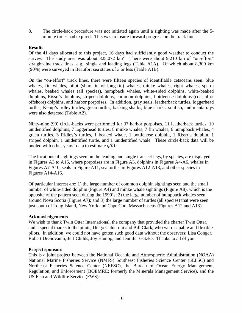
8. The circle-back procedure was not initiated again until a sighting was made after the 5-minute timer had expired. This was to insure forward progress on the track line.

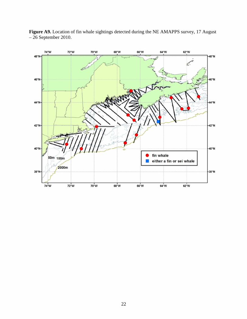
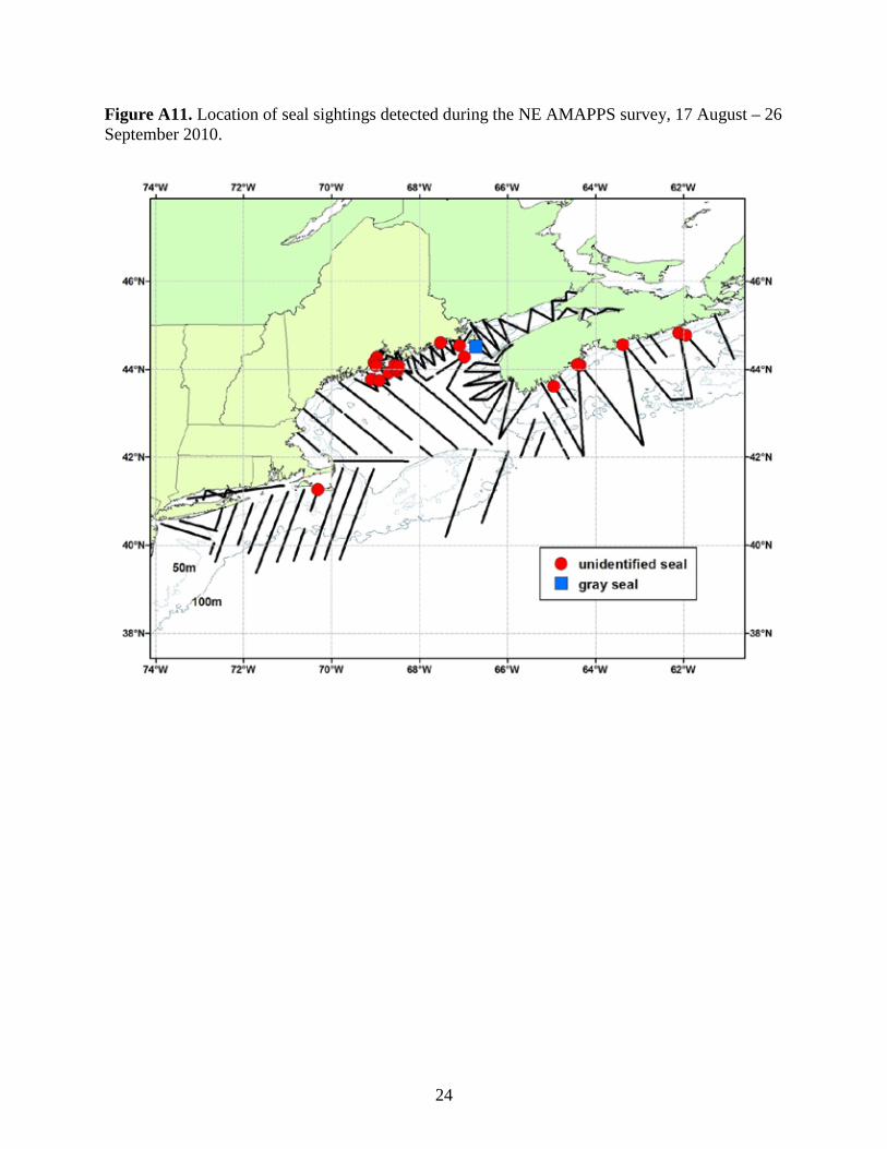
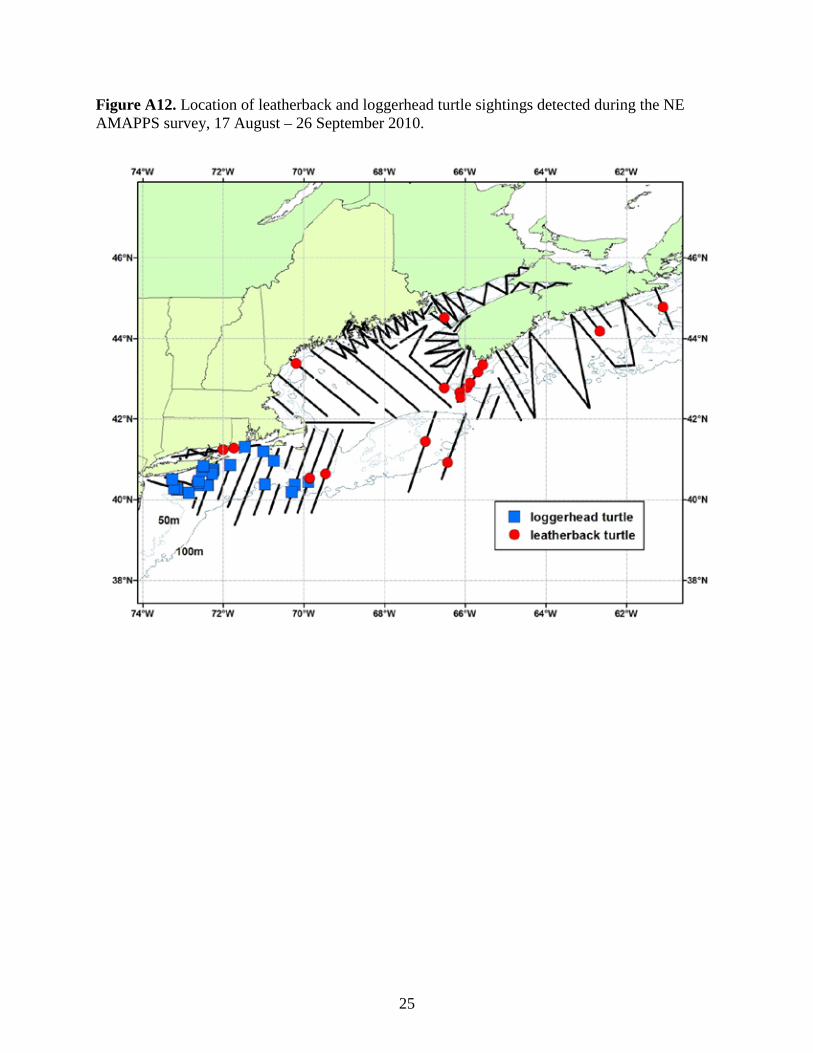
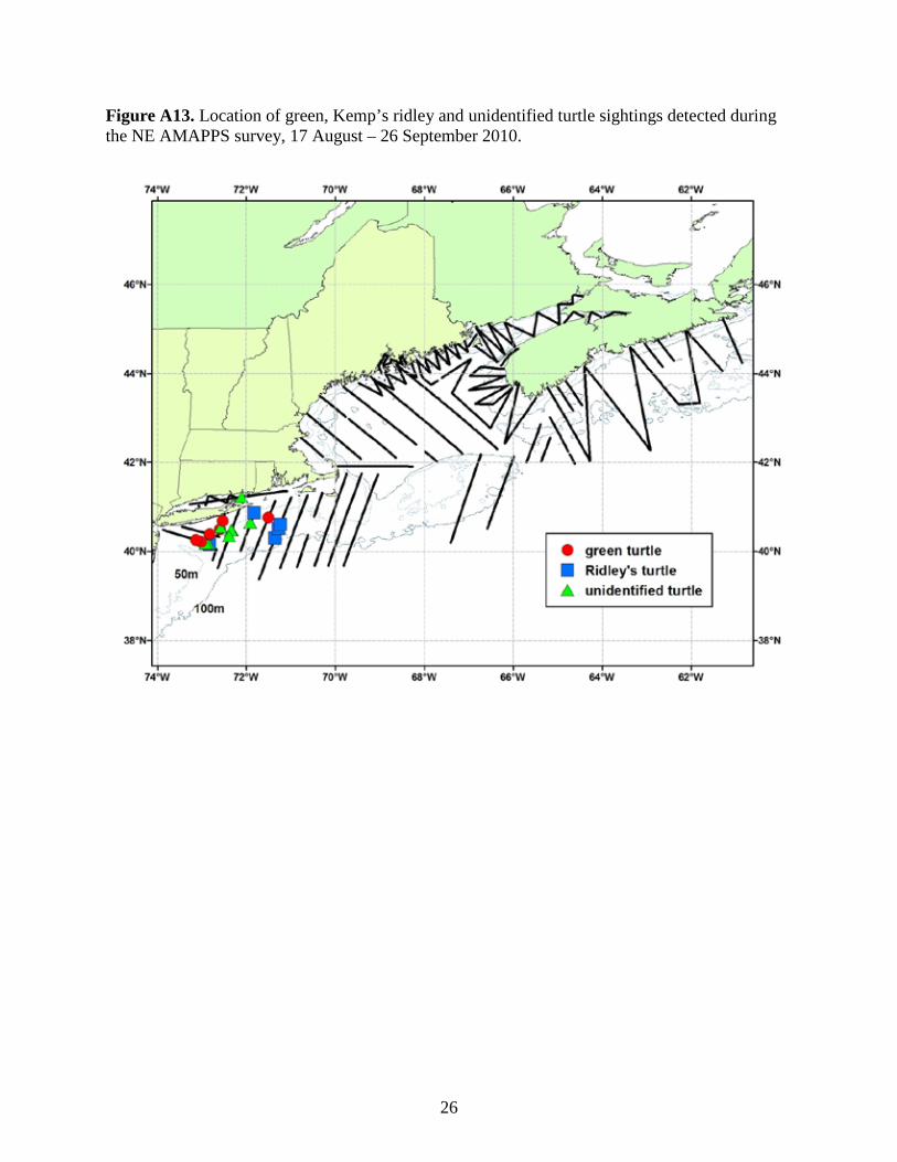
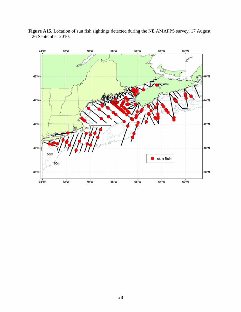
Results Of the 41 days allocated to this project, 16 days had sufficiently good weather to conduct the survey. The study area was about 325,072 km2. There were about 9,210 km of “on-effort” straight-line track lines, e.g., single and leading legs (Table A1A). Of which about 8,300 km (90%) were surveyed in Beaufort sea states of 3 or less (Table A1B). On the “on-effort” track lines, there were fifteen species of identifiable cetaceans seen: blue whales, fin whales, pilot (short-fin or long-fin) whales, minke whales, right whales, sperm whales, beaked whales (all species), humpback whales, white-sided dolphins, white-beaked dolphins, Risso’s dolphins, striped dolphins, common dolphins, bottlenose dolphins (coastal or offshore) dolphins, and harbor porpoises. In addition, gray seals, leatherback turtles, loggerhead turtles, Kemp’s ridley turtles, green turtles, basking sharks, blue sharks, sunfish, and manta rays were also detected (Table A2). Ninty-nine (99) circle-backs were performed for 37 harbor porpoises, 11 leatherback turtles, 10 unidentified dolphins, 7 loggerhead turtles, 8 minke whales, 7 fin whales, 6 humpback whales, 4 green turtles, 3 Ridley’s turtles, 1 beaked whale, 1 bottlenose dolphin, 1 Risso’s dolphin, 1 striped dolphin, 1 unidentified turtle, and 1 unidentified whale. These circle-back data will be pooled with other years’ data to estimate g(0). The locations of sightings seen on the leading and single transect legs, by species, are displayed in Figures A3 to A16, where porpoises are in Figure A3, dolphins in Figures A4-A6, whales in Figures A7-A10, seals in Figure A11, sea turtles in Figures A12-A13, and other species in Figures A14-A16. Of particular interest are: 1) the large number of common dolphin sightings seen and the small number of white-sided dolphin (Figure A4) and minke whale sightings (Figure A8), which is the opposite of the pattern seen during the 1990’s; 2) the large number of humpback whales seen around Nova Scotia (Figure A7); and 3) the large number of turtles (all species) that were seen just south of Long Island, New York and Cape Cod, Massachusetts (Figures A12 and A13). Acknowledgements We wish to thank Twin Otter International, the company that provided the charter Twin Otter, and a special thanks to the pilots, Diego Calderoni and Bill Clark, who were capable and flexible pilots. In addition, we could not have gotten such good data without the observers: Lisa Conger, Robert DiGiovanni, Jeff Childs, Joy Hampp, and Jennifer Gatzke. Thanks to all of you. Project sponsors This is a joint project between the National Oceanic and Atmospheric Administration (NOAA) National Marine Fisheries Service (NMFS) Southeast Fisheries Science Center (SEFSC) and Northeast Fisheries Science Center (NEFSC), the Bureau of Ocean Energy Management, Regulation, and Enforcement (BOEMRE; formerly the Minerals Management Service), and the US Fish and Wildlife Service (FWS).

11

Literature cited Hiby, L. 1999. The objective identification of duplicate sightings in aerial survey for porpoise.

Pages 179-189 in: Garner et al. (eds). Marine Mammal Survey and Assessment Methods. Balkema, Rotterdam.

List of tables Table A1. Lengths of on-effort track lines covered during NEFSC aerial abundance survey during 17 August – 26 September 2010.

A) Lengths of single, leading and trailing track lines (in km) and area (in km2). B) Lengths (km) of on-effort single and leading track lines surveyed during various Beaufort sea states.

Table A2. Number of groups and individual animals, and mean group size of the species detected during the leading and single legs, while on-effort during NEFSC aerial abundance survey during 17 August – 26 September 2010. List of figures Figure A1. Tracklines surveyed by the Twin Otter that were flown in various Beaufort sea states during 17 August – 26 September 2010. Figure A2. Diagram of how the circle-back technique was performed. Figure A3-A16. Location of sightings detected during the NE AMAPPS survey, 17 August – 26 September 2010. Figure A3. Harbor porpoises

Figure A4. White-sided and common dolphins Figure A5. Risso’s dolphins, pilot whales, and white-beaked dolphins Figure A6. Striped dolphins and unidentified dolphins Figure A7. Humpback whales Figure A8. Minke whales Figure A9. Fin whales Figure A10. Beaked, blue, right, sperm, and unidentified whales Figure A11. Seals Figure A12. Leatherback and loggerhead turtles Figure A13. Green, Kemp’s ridley and unidentified turtles Figure A14. Basking sharks Figure A15. Sun fish Figure A16. Blue shark, manta ray, tuna, unidentified shark and unidentified ray

12

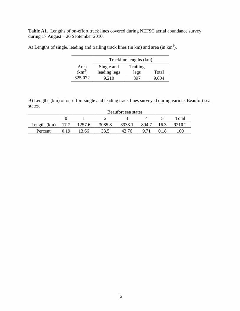
Table A1. Lengths of on-effort track lines covered during NEFSC aerial abundance survey during 17 August – 26 September 2010. A) Lengths of single, leading and trailing track lines (in km) and area (in km2).

Area (km2)

Trackline lengths (km) Single and

leading legs Trailing

legs Total 325,072 9,210 397 9,604

B) Lengths (km) of on-effort single and leading track lines surveyed during various Beaufort sea states.

Beaufort sea states

0 1 2 3 4 5 Total

Lengths(km) 17.7 1257.6 3085.8 3938.1 894.7 16.3 9210.2 Percent 0.19 13.66 33.5 42.76 9.71 0.18 100

13

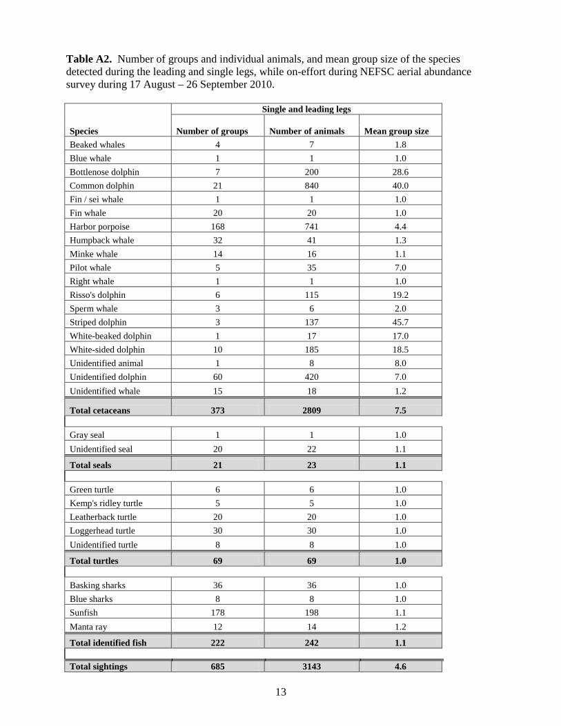
Table A2. Number of groups and individual animals, and mean group size of the species detected during the leading and single legs, while on-effort during NEFSC aerial abundance survey during 17 August – 26 September 2010.

Species

Single and leading legs

Number of groups Number of animals Mean group size Beaked whales 4 7 1.8 Blue whale 1 1 1.0 Bottlenose dolphin 7 200 28.6 Common dolphin 21 840 40.0 Fin / sei whale 1 1 1.0 Fin whale 20 20 1.0 Harbor porpoise 168 741 4.4 Humpback whale 32 41 1.3 Minke whale 14 16 1.1 Pilot whale 5 35 7.0 Right whale 1 1 1.0 Risso's dolphin 6 115 19.2 Sperm whale 3 6 2.0 Striped dolphin 3 137 45.7 White-beaked dolphin 1 17 17.0 White-sided dolphin 10 185 18.5 Unidentified animal 1 8 8.0 Unidentified dolphin 60 420 7.0 Unidentified whale 15 18 1.2

Total cetaceans 373 2809 7.5

Gray seal 1 1 1.0 Unidentified seal 20 22 1.1

Total seals 21 23 1.1

Green turtle 6 6 1.0 Kemp's ridley turtle 5 5 1.0 Leatherback turtle 20 20 1.0 Loggerhead turtle 30 30 1.0 Unidentified turtle 8 8 1.0

Total turtles 69 69 1.0

Basking sharks 36 36 1.0 Blue sharks 8 8 1.0 Sunfish 178 198 1.1 Manta ray 12 14 1.2

Total identified fish 222 242 1.1

Total sightings 685 3143 4.6

14

Figure A1. Tracklines surveyed by the Twin Otter that were flown in various Beaufort sea states during 17 August – 26 September 2010.

15

Figure A2. Diagram of how the circle-back technique was performed.

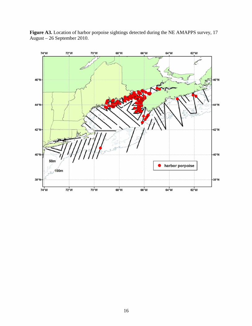
16

Figure A3. Location of harbor porpoise sightings detected during the NE AMAPPS survey, 17 August – 26 September 2010.

17

Figure A4. Location of white-sided and common dolphin sightings detected during the NE AMAPPS survey, 17 August – 26 September 2010.

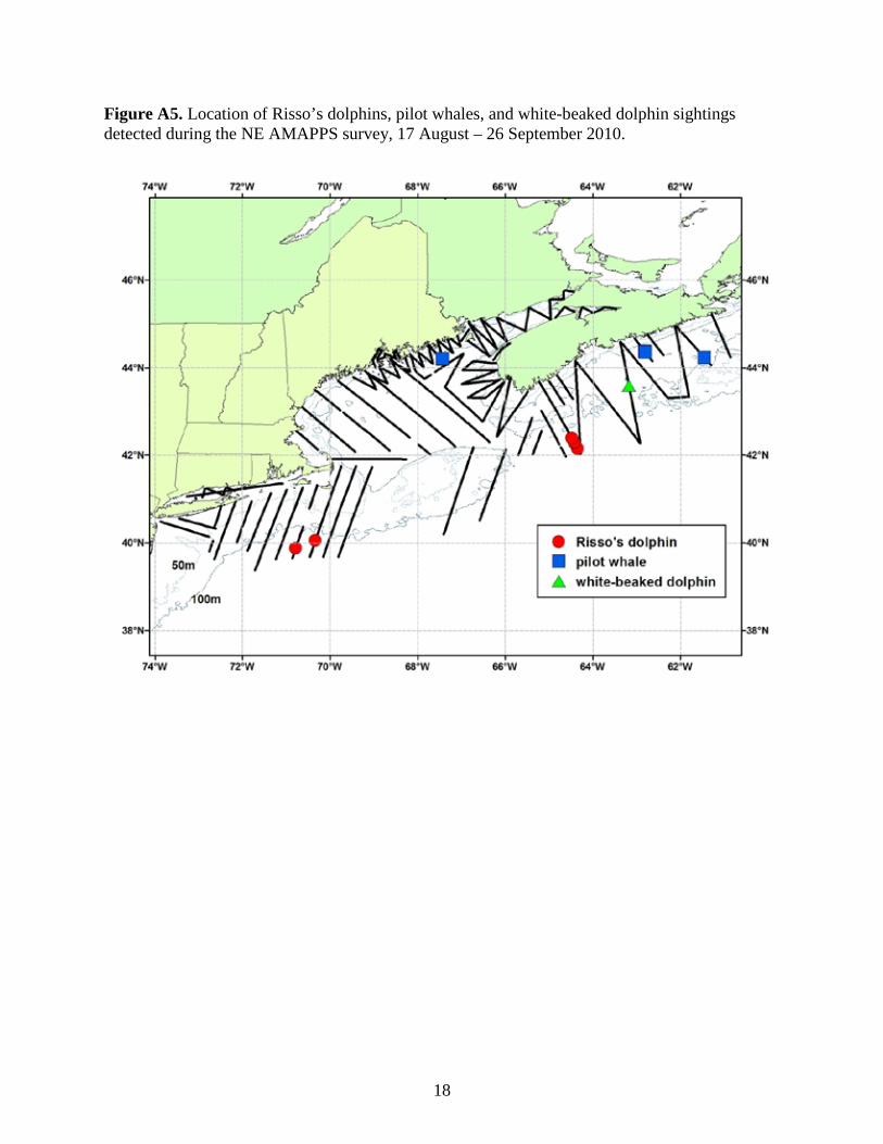
18

Figure A5. Location of Risso’s dolphins, pilot whales, and white-beaked dolphin sightings detected during the NE AMAPPS survey, 17 August – 26 September 2010.

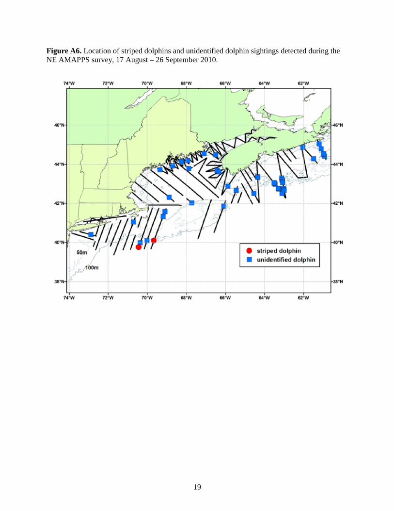
19

Figure A6. Location of striped dolphins and unidentified dolphin sightings detected during the NE AMAPPS survey, 17 August – 26 September 2010.

20

Figure A7. Location of humpback whale sightings detected during the NE AMAPPS survey, 17 August – 26 September 2010.

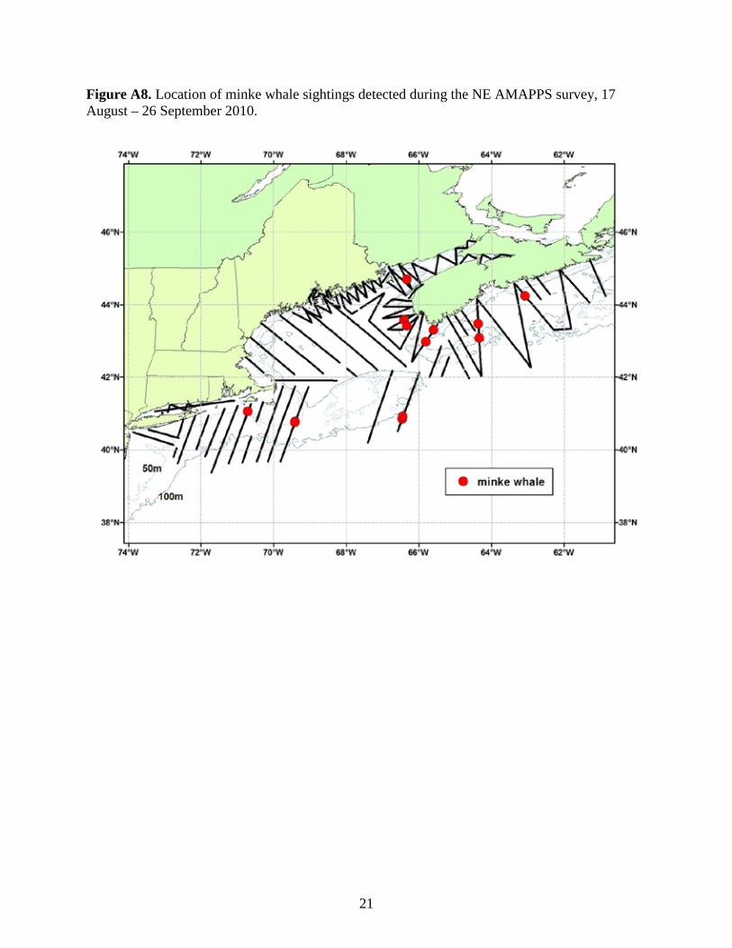
21

Figure A8. Location of minke whale sightings detected during the NE AMAPPS survey, 17 August – 26 September 2010.

22

Figure A9. Location of fin whale sightings detected during the NE AMAPPS survey, 17 August – 26 September 2010.

23

Figure A10. Location of beaked, blue, right, and sperm whales sightings, in addition to unidentified whale sightings detected during the NE AMAPPS survey, 17 August – 26 September 2010.

24

Figure A11. Location of seal sightings detected during the NE AMAPPS survey, 17 August – 26 September 2010.

25

Figure A12. Location of leatherback and loggerhead turtle sightings detected during the NE AMAPPS survey, 17 August – 26 September 2010.

26

Figure A13. Location of green, Kemp’s ridley and unidentified turtle sightings detected during the NE AMAPPS survey, 17 August – 26 September 2010.

27

Figure A14. Location of basking shark sightings detected during the NE AMAPPS survey, 17 August – 26 September 2010.

28

Figure A15. Location of sun fish sightings detected during the NE AMAPPS survey, 17 August – 26 September 2010.

29

Figure A16. Location of blue shark, manta ray, tuna, unidentified shark and unidentified ray sightings detected during the NE AMAPPS survey, 17 August – 26 September 2010.

30

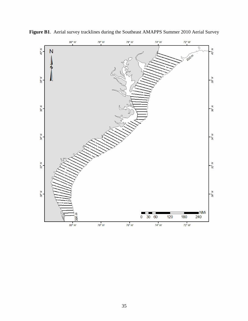
Appendix B: Southern leg of the AMAPPS aerial line-transect abundance survey, summer 2010: Southeast Fisheries Science Center Lance P. Garrison1, Kevin P. Barry2, Keith D. Mullin2 1Southeast Fisheries Science Center, 75 Virginia Beach Dr., Miami FL 33149 2Southeast Fisheries Science Center, 3209 Frederic St., Pascagoula, MS 39567 Summary As part of the AMAPPS program, the Southeast Fisheries Science Center conducted an aerial survey of continental shelf waters along the US East Coast from Cape Canaveral, Florida to Cape May, New Jersey. The survey was conducted along tracklines oriented perpendicular to the shoreline that were latitudinally spaced 20 km apart. The survey was conducted aboard a Twin Otter aircraft at an altitude of 600 feet (183 m) and a speed of 110 knots. The survey was designed for analysis using Distance sampling and a two-team (independent observer) approach to correct for visibility bias in resulting abundance estimates. The survey was conducted between 24 July and 14 August 2010. During that period, flights were conducted on 12 days with the remaining days lost due to poor weather conditions. A total of 7,944 km of trackline were surveyed on effort during 86 flight hours. Six species of marine mammals were identified, with the majority being bottlenose dolphins (127 groups sighted totaling 1,541 animals). Four species of sea turtles were identified, with the majority being loggerhead turtles (563 groups totaling 742 animals). The data collected from this survey will be analyzed to estimate the abundance and spatial distribution of mammals and turtles along the US east coast. Objectives The goal of this survey was to conduct line-transect surveys using the Distance sampling approach to estimate the abundance and spatial distribution of marine mammals and turtles in waters over the continental shelf (shoreline to 200m isobaths) from Cape Canaveral, Florida to Cape May, New Jersey. Methods The survey was conducted aboard a DeHavilland Twin Otter DHC-6 flying at an altitude of 183m (600 ft) above the water surface and a speed of approximately 200 kph (110 knots). Surveys were typically flown only when wind speeds were less than 20 knots or approximately sea state 4 or less on the Beaufort scale. The survey was conducted along tracklines oriented perpendicular to the shoreline and spaced latitudinally at approximately 20 km intervals from a random start point (Figure B1). There were two pilots and six scientists onboard the airplane. The scientists operated as two teams to implement the independent observer approach to correct for visibility bias (Laake and Borchers 2004). The forward team (Team 1) consisted of two observers stationed in bubble windows on either side of the airplane and an associated data recorder. The bubble windows allowed downward visibility including the trackline. The aft team (Team 2) consisted of a belly observer looking straight down through a belly port, an observer stationed on one side of the aircraft observing through a large window, and a dedicated data recorder. For the aft team, the side observer did not have complete visibility of the trackline, and the belly observer had

31

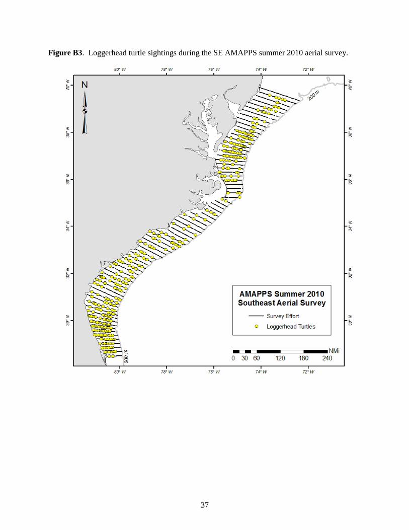
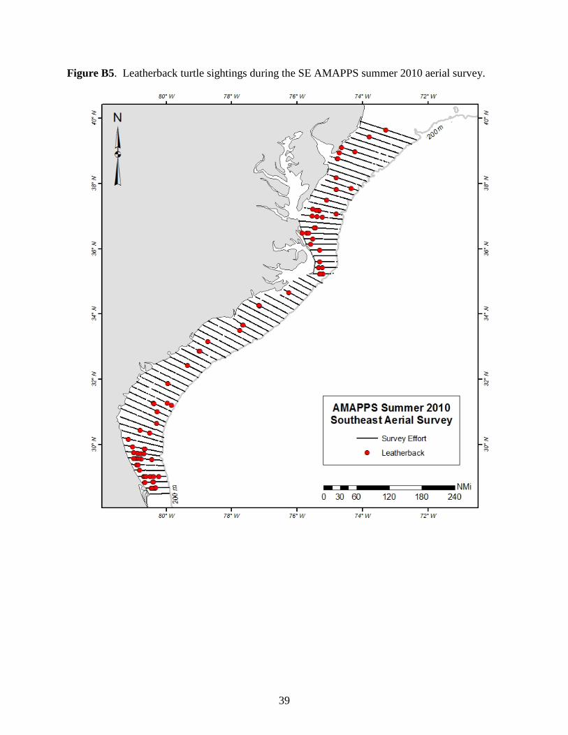
visibility of only approximately 30˚ on either side of the line. The side window observer alternated sides of the aircraft each day. The two observer teams operated on independent intercom channels so that they were not able to cue one another to sightings. Data was recorded by each team’s observer onto a laptop computer running data acquisition software that recorded GPS location, environmental conditions entered by the observer team (e.g., sea state, water color, glare, sun penetration, visibility, etc.), effort information, and surface water temperature. Surface water temperature was measured by an infra-red temperature probe deployed in a port just forward of the belly window. During on effort periods (e.g., level flight at survey altitude and speed), observers searched visually from the trackline (0˚) to approximately 50˚ above vertical. When a turtle, mammal, or other organism was observed, the observer waited until it was perpendicular to the aircraft and then measured the angle to the organism (or the center of the group) using a digital inclinometer or recorded the angle in 10˚ intervals based upon markings on the windows. The belly observer only reported the 10˚ interval for the sighting. Fish species were recorded opportunistically. Sea turtle sightings were recorded independently, without communication, by each team. For marine mammal sightings, if the sighting was made initially by the forward team, they waited until it was aft of the airplane to allow the aft team an opportunity to observe the group before notifying the pilots to circle over the group. Once both teams had the opportunity to observe the group, the observers asked the pilots to break effort and circle the group. The aircraft circled over the majority of the marine mammal groups sighted to verify species identification and group sizes and to take photographs. The data recorders indicated at the time of the sighting whether or not the group was recorded by one or both teams. After the survey, the turtle data were reviewed to identify duplicate sightings by the two teams based upon time, location, and position relative to the trackline. Results The survey was conducted during 24 July – 14 August 2010, but survey flights could only be conducted on 12 days during that period due to weather conditions, mechanical issues, or transits between cities. A total of 86.1 flight hours were used, and a total of 7,944 km of trackline were covered on effort along 75 tracklines (Figure B1, Table B1). The average sea state during the survey was 2.6 on the Beaufort scale with the vast majority of the survey effort flown in sea states of 2 or 3 (Figure B2). There were a total of 1,234 unique sightings of sea turtles for a total of 1,502 individuals. Turtles were identified as loggerhead turtles, green turtles, Kemp’s ridley turtles, leatherback turtles, and unidentified hardshells (Table B2). Of these, the majority of turtle sightings were loggerhead turtles (Figure B3). A greater number of green turtles were observed north of Cape Hatteras, NC (Figure B4), and leatherback turtles were observed primarily just north of Cape Canaveral, FL and north of Cape Hatteras, NC (Figure B5). There were a total of 181 groups of marine mammals sighted for a total of 2,567 individuals. The primary species observed was bottlenose dolphins; however, there were also observations of

32

several other taxa including Atlantic spotted dolphins, common dolphins, Risso’s dolphins, pilot whales, and fin whales (Table B3, Figures B6-B8). As in previous studies, bottlenose dolphins occurred continuously across the continental shelf south of Cape Hatteras where the offshore and coastal morphotypes overlapped in space. However, north of Cape Hatteras, there was a distinct break in bottlenose dolphin distribution which was associated with the separation of these populations in this region (Figure B6). Pilot whales and other taxa associated with the shelf break were observed on the outer ends of tracklines north of Cape Hatteras, NC (Figure B8). Fish species sighted included primarily sharks, rays, and sunfish (Figure B9). Literature cited Laake, J.L. and Borchers, D.L. 2004. Methods for incomplete detection at distance zero. In:

Advanced Distance Sampling. Buckland, S.T., Anderson, D.R., Burnham, K.P., Laake, J.L., and Thomas, L. (eds.). Oxford University Press, 411 pp.

33

Table B1. Daily summary of survey effort and protected species sightings.

Date Flight Hours Effort (km) Marine Mammal

Sightings Turtle

Sightings Average Sea

State 7/24/2010 7.08 804.9 19 95 2.8 7/25/2010 9.17 910.2 29 339 2.5 7/26/2010 2.32 Weather/Transit 7/27/2010 6.08 507.1 21 69 2.4 7/28/2010 6.45 679.2 19 86 2 7/29/2010 6.50 675.8 13 39 2.8 7/30/2010 0.00 Weather 7/31/2010 1.48 Weather/Transit 8/1/2010 2.77 125.7 2 4 2.4 8/2/2010 0.00 Weather 8/3/2010 4.48 500.5 7 38 2.8 8/4/2010 8.17 805.7 13 24 3 8/5/2010 1.58 Weather/Transit 8/6/2010 0.00 Weather 8/7/2010 8.25 806.2 13 106 2.9 8/8/2010 0.52 Weather 8/9/2010 8.18 799.5 20 296 1.9 8/10/2010 5.78 482.6 12 41 3.4 8/11/2010 7.33 846.8 13 95 2.8 8/12/2010 0.00 Weather 8/13/2010 0.00 Weather 8/14/2010 0.00 Weather

Total 86.14 7944.1 181 1232 2.6

34

Table B2. Summary of sea turtle sightings

Species Number of groups

Number of animals

Green Turtle 107 112

Unid. Hardshell 451 531

Kemp's ridley 19 20

Leatherback 94 97

Loggerhead 563 742

Total 1234 1502

Table B3. Summary of marine mammal sightings

Species Number of groups

Number of animals

Atlantic spotted dolphin 15 364

Bottlenose Dolphin 127 1541

Bottlenose/Atl Spotted Dolphin 7 127

Common Dolphin 2 115

Fin Whale 4 5

Pilot Whale 4 208

Risso's Dolphin 5 102

Stenella sp. 2 10

Unid. Baleen Whale 1 2

Unid. Dolphin 10 74

Unid. Odonocete 3 11

Unid. Sm. Whale 1 8

Total 181 2567

35

Figure B1. Aerial survey tracklines during the Southeast AMAPPS Summer 2010 Aerial Survey

36

Figure B2. Beaufort sea states during Southeast AMMAPS aerial survey.

37

Figure B3. Loggerhead turtle sightings during the SE AMAPPS summer 2010 aerial survey.

38

Figure B4. Other hardshell turtle sightings during the SE AMAPPS summer 2010 aerial survey.

39

Figure B5. Leatherback turtle sightings during the SE AMAPPS summer 2010 aerial survey.

40

Figure B6. Bottlenose dolphin sightings during the SE AMAPPS summer 2010 aerial survey.

41

Figure B7. Other dolphin sightings during the SE AMAPPS summer 2010 aerial survey.

42

Figure B8. Large and small whale sightings during the SE AMAPPS summer 2010 aerial survey.

43

Figure B9. Fish sightings during the SE AMAPPS summer 2010 aerial survey.

44

Appendix C: Northern sea turtle tagging study, summer 2010: Northeast Fisheries Science Center Heather Haas1, Ron Smolowitz2, Matthew Weeks2, Henry Milliken1, Eric Matzen3 1Northeast Fisheries Science Center, 166 Water St., Woods Hole, MA 02543 2Coonamessett Farm Foundation, 277 Hatchville Road, E. Falmouth, MA 02536 3Integrated Statistics, 16 Sumner St., Woods Hole, MA 02543 Background This tagging study is part of the AMAPPS (Atlantic Marine Assessment Program for Protected Species) project, which is a large, multi-agency initiative to provide a comprehensive assessment of marine mammal, sea turtle, and seabird abundance and spatial distribution in US waters of the western North Atlantic Ocean. The goal of the AMAPPS initiative is to develop models and associated tools to provide seasonal, spatially-explicit density estimates of marine mammals, sea turtles, and seabirds in the western north Atlantic. Data will be collected on the seasonal distribution and abundance of these taxa using direct aerial and shipboard surveys conducted by scientists from the National Marine Fisheries Service and the US Fish and Wildlife Service. Concurrently, telemetry studies, passive acoustic monitoring, and development of alternative survey methodologies are also being conducted under AMAPPS. The telemetry data will be used to develop corrections for availability bias in the abundance estimates and to collect additional data on habitat use and life history, residence time, and frequency of use. Data collection for this study is planned to occur over multiple years. As part of the AMAPPS project, satellite tags were deployed on immature loggerhead sea turtles captured in offshore Mid-Atlantic waters. The US Mid-Atlantic region is an important foraging ground for loggerhead sea turtles, but due to complications involved with locating and capturing these immature turtles on their offshore foraging grounds, relatively little is known about the large, immature turtles that occupy the neritic offshore Mid-Atlantic region. Methods The Northeast Fisheries Science Center (NEFSC) partnered with Coonamessett Farm Foundation (with the assistance of Viking Village Fisheries and the F/V Kathy Ann), who provided the vessel, crew, and at-sea scientific personnel. This partnership allowed loggerheads to be sampled in their offshore Mid-Atlantic foraging grounds. In August and September of 2010, the F/V Kathy Ann (95 ft commercial fishing vessel rigged with crow’s nest, rising 60 ft above the waterline) was used to locate immature loggerheads in an area known to have overlap between large, immature loggerheads and commercial fishing activity (roughly 50-100 miles offshore of Delaware and New Jersey). After an animal was located, a small boat (14 ft) was deployed to capture loggerheads using a large dipnet. The Sea Mammal Research Unit’s (SMRU) Fastloc GPS Satellite Relay Data Loggers (SRDLs) were attached with epoxy to the second central carapace scute. Captured turtles were also measured (curved carapace length, CCL), photographed, biopsied, and flipper and PIT tagged.

45

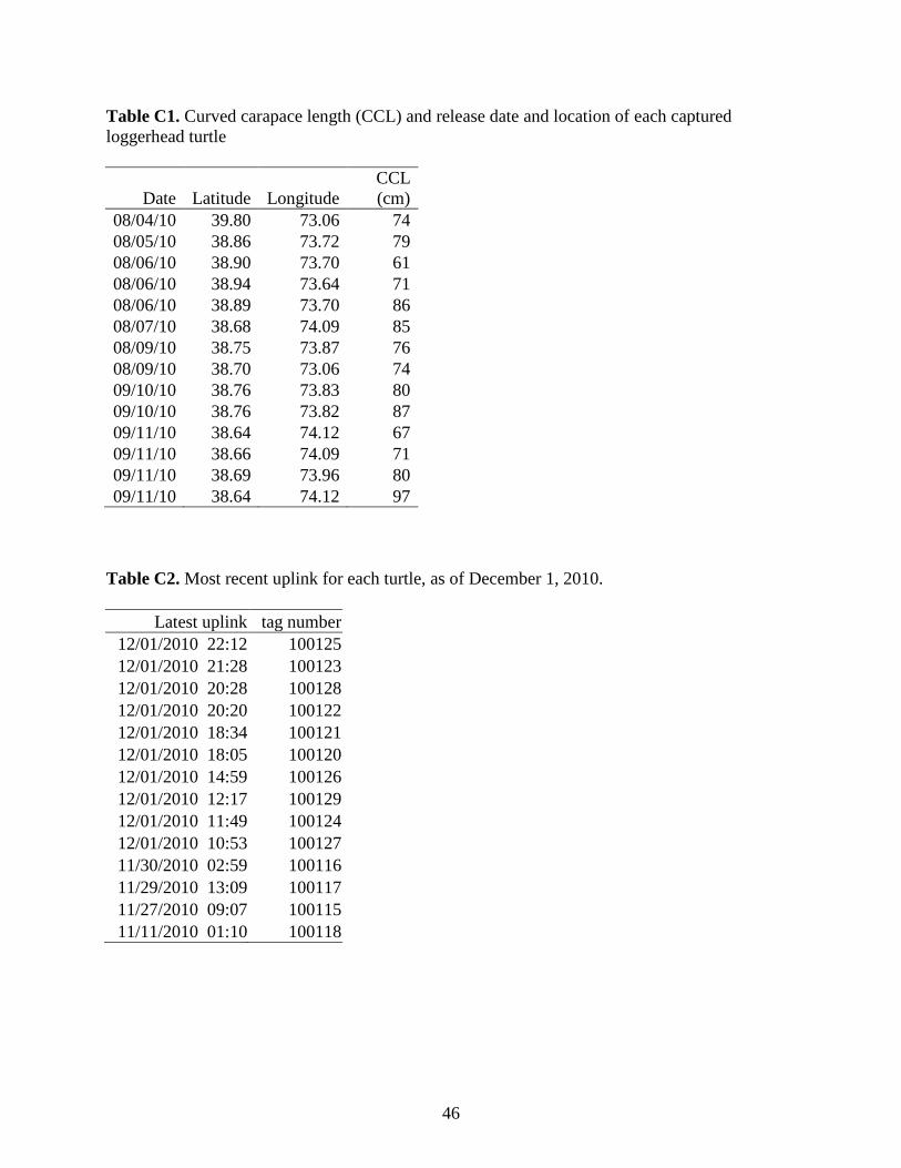
Specifications for the SMRU Fastloc GPS Satellite Relay Data Loggers are provided in Appendix C2. The Fastloc GPS supplies highly accurate locations. The tag also uses precision wet/dry, pressure, and temperature sensors to form individual dive (max depth, shape, time at depth, etc.) records along with temperature profiles and binned summary records. The SMRU tag stores information in its memory and then relays an unbiased sample of detailed individual dive records and summary records. Results A total of 14 immature loggerhead sea turtles (61 - 97 cm CCL) were captured and satellite-tagged, primarily offshore of New Jersey and Delaware (Table C1). The dates and times of the most recent uplink for each tag, according to the SMRU website as of December 1, 2010, are listed in Table C2. At that time, 13 of the 14 tags were actively transmitting (messages sent within the last week); however, 5 of the 13 active tags were not transmitting reliable location information.

The satellite-relayed data are currently stored in two ways. Location data are downloaded daily to the publically-accessible website (http://www.seaturtle.org/tracking/?project_id=537). Figure C1 shows the composite seaturtle.org map of these tags for the entire study period. The detailed GPS location, temperature, and dive data are downloaded daily to a password-protected SMRU website and intermittently uploaded to a NEFSC Oracle database. As of December 1, 2010, the NEFSC Oracle database included approximately 10,000 locations, 10,000 individual dive profiles, and 3,000 six-hour summaries of depth usage. From their initial capture location, the tagged loggerheads moved south along the continental shelf and, as of December 1, 2010, were off of North Carolina (Figure C1). Acknowledgements We wish to thank the following people for their assistance with the satellite tagging portion of this project: James Gutowski, Mike Francis, Raymond Hines, Elizabeth Josephson, Cory Karch, Tyler Larson, Paul Salon, and Joseph Wager. Project sponsors This is a joint project between the National Oceanic and Atmospheric Administration (NOAA) National Marine Fisheries Service (NMFS) Southeast Fisheries Science Center (SEFSC) and Northeast Fisheries Science Center (NEFSC), the Bureau of Ocean Energy Management, Regulation, and Enforcement (BOEME; formerly the Minerals Management Service), the US Fish and Wildlife Service (FWS), and the sea scallop industry through their research set aside program. This telemetry work is being conducted in cooperation with the Coonamessett Farm Foundation with the assistance of Viking Village Fisheries and the F/V Kathy Ann.

46

Table C1. Curved carapace length (CCL) and release date and location of each captured loggerhead turtle

Date Latitude Longitude CCL (cm)

08/04/10 39.80 73.06 74 08/05/10 38.86 73.72 79 08/06/10 38.90 73.70 61 08/06/10 38.94 73.64 71 08/06/10 38.89 73.70 86 08/07/10 38.68 74.09 85 08/09/10 38.75 73.87 76 08/09/10 38.70 73.06 74 09/10/10 38.76 73.83 80 09/10/10 38.76 73.82 87 09/11/10 38.64 74.12 67 09/11/10 38.66 74.09 71 09/11/10 38.69 73.96 80 09/11/10 38.64 74.12 97

Table C2. Most recent uplink for each turtle, as of December 1, 2010.

Latest uplink tag number 12/01/2010 22:12 100125 12/01/2010 21:28 100123 12/01/2010 20:28 100128 12/01/2010 20:20 100122 12/01/2010 18:34 100121 12/01/2010 18:05 100120 12/01/2010 14:59 100126 12/01/2010 12:17 100129 12/01/2010 11:49 100124 12/01/2010 10:53 100127 11/30/2010 02:59 100116 11/29/2010 13:09 100117 11/27/2010 09:07 100115 11/11/2010 01:10 100118

47

Figure C1. Location information as displayed by seaturtle.org on December 1, 2010. The stars indicate the last recorded location.

48

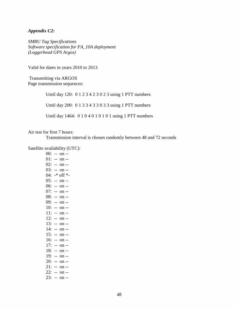
Appendix C2: SMRU Tag Specifications Software specification for FA_10A deployment (Loggerhead GPS Argos) Valid for dates in years 2010 to 2013 Transmitting via ARGOS Page transmission sequences: Until day 120: 0 1 2 3 4 2 3 0 2 3 using 1 PTT numbers Until day 200: 0 1 3 3 4 3 3 0 3 3 using 1 PTT numbers Until day 1464: 0 1 0 4 0 1 0 1 0 1 using 1 PTT numbers Air test for first 7 hours: Transmission interval is chosen randomly between 48 and 72 seconds Satellite availability (UTC): 00: -- on -- 01: -- on -- 02: -- on -- 03: -- on -- 04: -* off *- 05: -- on -- 06: -- on -- 07: -- on -- 08: -- on -- 09: -- on -- 10: -- on -- 11: -- on -- 12: -- on -- 13: -- on -- 14: -- on -- 15: -- on -- 16: -- on -- 17: -- on -- 18: -- on -- 19: -- on -- 20: -- on -- 21: -- on -- 22: -- on -- 23: -- on --

49

Transmission targets: 50000 transmissions after 200 days 7000 transmissions after 365 days In Haul outs: ON (one tx every 44 secs) for first 1 day then cycling OFF for 0, ON for 1 day Check sensors every 4 secs when near surface (shallower than 6m), Check wet/dry every 1 sec Consider wet/dry sensor failed if wet for 30 days or dry for 99 days Dives start when wet and below 1.5m for 20 secs and end when dry, or above 1.5m Do not separate 'Deep' dives A cruise begins if there has been no dive for 15 mins A haulout begins when dry for 6 mins and ends when wet for 40 secs Dive shape (normal dives): 5 points per dive using broken-stick algorithm Dive shape (deep dives): none CTD profiles: Max 250 dbar up to 2 dbar in 1 dbar bins. Temperature: Collected, Stored. Conductivity: Not collected. Salinity: Not collected. Fluorescence: Not collected. Construct a single profile for each 4-hour period. During profile, sample CTD sensor every 4 seconds. Each profile contains 10 cut points consisting of 0 fixed points, minimum depth,

maximum depth, 8 broken-stick points GPS fixes: Number of GPS attempts allowed: 5000 (then increase interval to 0x normal) Cut-off date for GPS attempts: 120 days (then increase interval to 0x normal) Discard results with fewer than 5 satellites Processing timeout: 30 secs Haul outs: Increase interval to 12x normal after first success in haul out TRANSMISSION BUFFERS (in RAM):

Dives in groups of 2 (5.55556 days @ 10mins/dive): 400 = 1600 bytes No 'deep' dives Haul outs: 30 = 120 bytes 6-hour Summaries in groups of 2 (15 days): 30 = 120 bytes No Timelines Cruises: 30 = 120 bytes

50

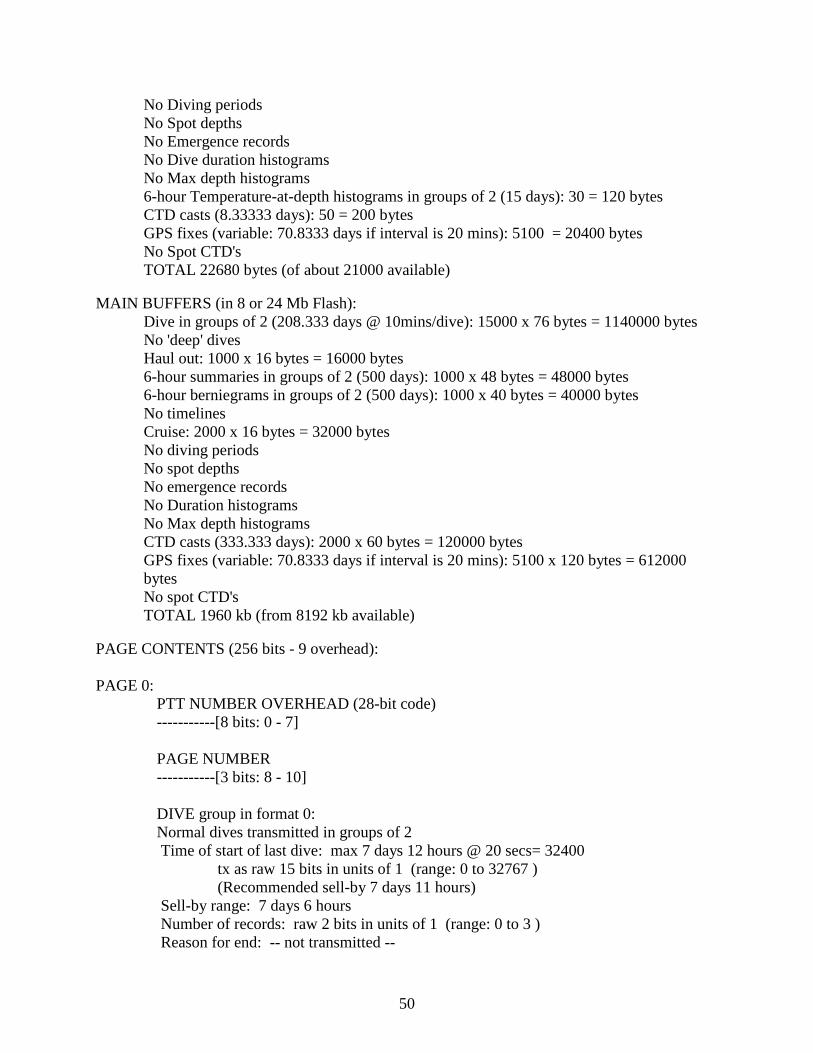
No Diving periods No Spot depths No Emergence records No Dive duration histograms No Max depth histograms 6-hour Temperature-at-depth histograms in groups of 2 (15 days): 30 = 120 bytes CTD casts (8.33333 days): 50 = 200 bytes GPS fixes (variable: 70.8333 days if interval is 20 mins): 5100 = 20400 bytes No Spot CTD's TOTAL 22680 bytes (of about 21000 available)

MAIN BUFFERS (in 8 or 24 Mb Flash):

Dive in groups of 2 (208.333 days @ 10mins/dive): 15000 x 76 bytes = 1140000 bytes No 'deep' dives Haul out: 1000 x 16 bytes = 16000 bytes 6-hour summaries in groups of 2 (500 days): 1000 x 48 bytes = 48000 bytes 6-hour berniegrams in groups of 2 (500 days): 1000 x 40 bytes = 40000 bytes No timelines Cruise: 2000 x 16 bytes = 32000 bytes No diving periods No spot depths No emergence records No Duration histograms No Max depth histograms CTD casts (333.333 days): 2000 x 60 bytes = 120000 bytes GPS fixes (variable: 70.8333 days if interval is 20 mins): 5100 x 120 bytes = 612000 bytes No spot CTD's TOTAL 1960 kb (from 8192 kb available)

PAGE CONTENTS (256 bits - 9 overhead): PAGE 0: PTT NUMBER OVERHEAD (28-bit code) -----------[8 bits: 0 - 7] PAGE NUMBER -----------[3 bits: 8 - 10] DIVE group in format 0: Normal dives transmitted in groups of 2 Time of start of last dive: max 7 days 12 hours @ 20 secs= 32400 tx as raw 15 bits in units of 1 (range: 0 to 32767 ) (Recommended sell-by 7 days 11 hours) Sell-by range: 7 days 6 hours Number of records: raw 2 bits in units of 1 (range: 0 to 3 ) Reason for end: -- not transmitted --

51

Group number: -- not transmitted -- Max depth: -- not transmitted -- Dive duration: Lookup with 64 bins:

<20,20-30,30-40,40-50,50-60,60-80,80-100,100-120,120-140,140-160,160-180,180-240,240-300,300-360,360-420,420-480,480-600,600-720,720-840,840-960,960-1080,1080-1200,1200-1320,1320-1440,1440-1560,1560-1680,1680-1800,1800-2100,2100-2400,2400-2700,2700-3000,3000-3300,3300-3600,3600-3900,3900-4200,4200-4500,4500-4800,4800-5100,5100-5400,5400-5700,5700-6000,6000-6300,6300-6600,6600-6900,6900-7200,7200-7800,7800-8400,8400-9000,9000-9600,9600-10200,10200-10800,10800-12000,12000-13200,13200-14400,14400-16200,16200-18000,18000-19800,19800-21600,21600-28800,28800-36000,36000-43200,43200-54000,54000-64800, >64800 in units of 1 s (range: 0 to 64800 s)

Mean speed: -- not transmitted -- Profile data (5 depths/times, 0 speeds): Depth profile: Lookup with 64 bins:

<1,1-2,2-3,3-4,4-5,5-6,6-7,7-8,8-9,9-10,10-11,11-12,12-13,13-14,14-15,15-16,16-17,17-18,18-19,19-20,20-22,22-24,24-26,26-28,28-30,30-32,32-34,34-36,36-38,38-40,40-42,42-44,44-46,46-48,48-50,50-52,52-54,54-56,56-58,58-60,60-62,62-64,64-66,66-68,68-70,70-75,75-80,80-85,85-90,90-95,95-100,100-110,110-120,120-130,130-140,140-150,150-160,160-170,170-180,180-190,190-200,200-220,220-240, >240 in units of 0.1 m (range: 0 to 240 m)

Profile times: raw 9 bits in units of 1.95695 permille (range: 0 to 1000 permille) Speed profile: -- not transmitted -- Residual: -- not transmitted -- Calculation time: -- not transmitted -- Surface duration: odlog 2/4 in units of 4 s (range: 0 to 942 s) cf. cruise starts after 15 mins (900 secs) Dive area: raw 9 bits in units of 1.95695 permille (range: 0 to 1000 permille) -----------[209 bits: 11 - 219] CRUISE group in format 0: Number of records: raw 1 bits in units of 1 (range: 0 to 1) Cruise number: wraparound 6 bits in units of 1 (range: 0 to 63) Start time: -- not transmitted -- End time: max 5 days 12 hours @ 2 mins= 3960 tx as raw 12 bits in units of 1 (range: 0 to 4095) (recommended sell-by 5 days 11 hours) Sell-by range: 5 days 4 hours Duration: odlog 2/6 in units of 90 s (range: 0 to 85995 s) cf. Max duration is 1 day Speed: -- not transmitted -- Reason for end: -- not transmitted -- -----------[27 bits: 220 - 246] Available bits used exactly

52

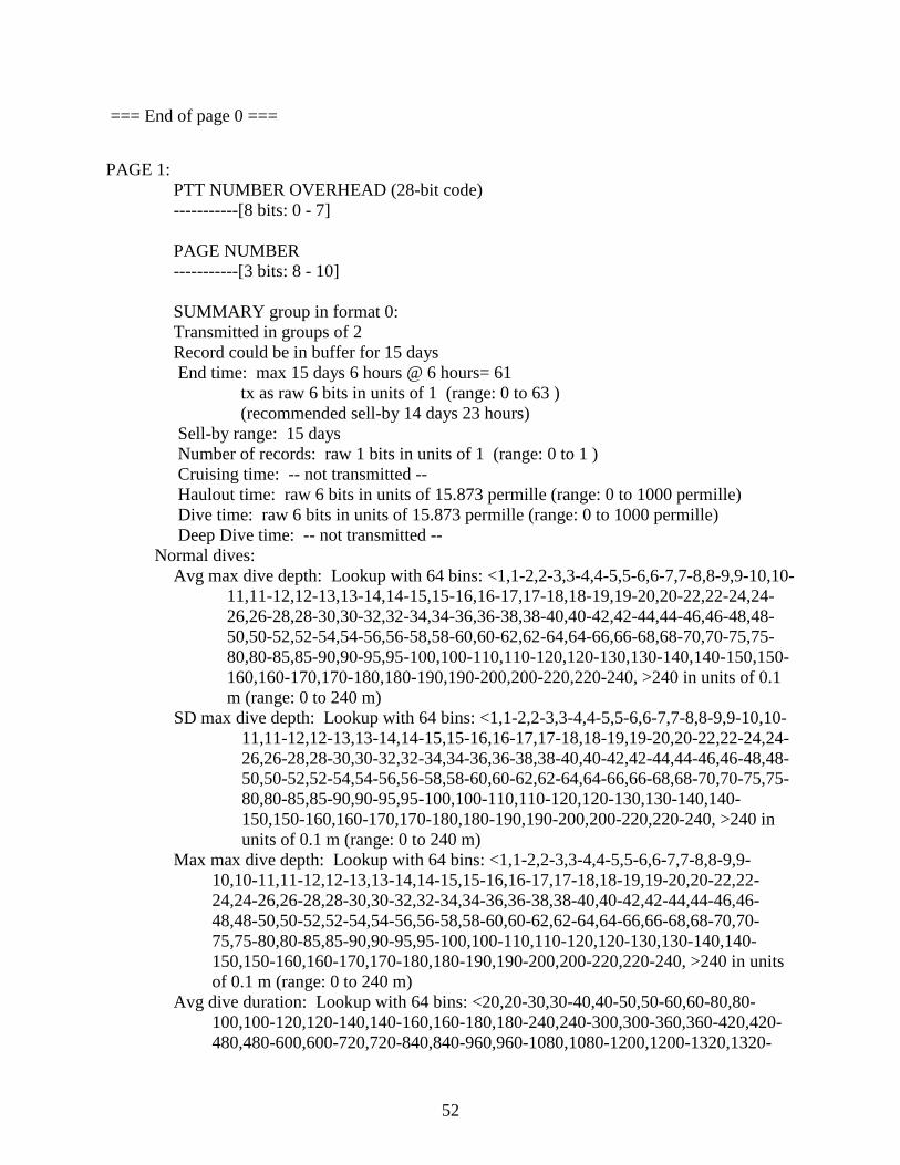
=== End of page 0 === PAGE 1: PTT NUMBER OVERHEAD (28-bit code) -----------[8 bits: 0 - 7] PAGE NUMBER -----------[3 bits: 8 - 10] SUMMARY group in format 0: Transmitted in groups of 2 Record could be in buffer for 15 days End time: max 15 days 6 hours @ 6 hours= 61 tx as raw 6 bits in units of 1 (range: 0 to 63 ) (recommended sell-by 14 days 23 hours) Sell-by range: 15 days Number of records: raw 1 bits in units of 1 (range: 0 to 1 ) Cruising time: -- not transmitted -- Haulout time: raw 6 bits in units of 15.873 permille (range: 0 to 1000 permille) Dive time: raw 6 bits in units of 15.873 permille (range: 0 to 1000 permille) Deep Dive time: -- not transmitted -- Normal dives:

Avg max dive depth: Lookup with 64 bins: <1,1-2,2-3,3-4,4-5,5-6,6-7,7-8,8-9,9-10,10-11,11-12,12-13,13-14,14-15,15-16,16-17,17-18,18-19,19-20,20-22,22-24,24-26,26-28,28-30,30-32,32-34,34-36,36-38,38-40,40-42,42-44,44-46,46-48,48-50,50-52,52-54,54-56,56-58,58-60,60-62,62-64,64-66,66-68,68-70,70-75,75-80,80-85,85-90,90-95,95-100,100-110,110-120,120-130,130-140,140-150,150-160,160-170,170-180,180-190,190-200,200-220,220-240, >240 in units of 0.1 m (range: 0 to 240 m)

SD max dive depth: Lookup with 64 bins: <1,1-2,2-3,3-4,4-5,5-6,6-7,7-8,8-9,9-10,10-11,11-12,12-13,13-14,14-15,15-16,16-17,17-18,18-19,19-20,20-22,22-24,24-26,26-28,28-30,30-32,32-34,34-36,36-38,38-40,40-42,42-44,44-46,46-48,48-50,50-52,52-54,54-56,56-58,58-60,60-62,62-64,64-66,66-68,68-70,70-75,75-80,80-85,85-90,90-95,95-100,100-110,110-120,120-130,130-140,140-150,150-160,160-170,170-180,180-190,190-200,200-220,220-240, >240 in units of 0.1 m (range: 0 to 240 m)

Max max dive depth: Lookup with 64 bins: <1,1-2,2-3,3-4,4-5,5-6,6-7,7-8,8-9,9-10,10-11,11-12,12-13,13-14,14-15,15-16,16-17,17-18,18-19,19-20,20-22,22-24,24-26,26-28,28-30,30-32,32-34,34-36,36-38,38-40,40-42,42-44,44-46,46-48,48-50,50-52,52-54,54-56,56-58,58-60,60-62,62-64,64-66,66-68,68-70,70-75,75-80,80-85,85-90,90-95,95-100,100-110,110-120,120-130,130-140,140-150,150-160,160-170,170-180,180-190,190-200,200-220,220-240, >240 in units of 0.1 m (range: 0 to 240 m)

Avg dive duration: Lookup with 64 bins: <20,20-30,30-40,40-50,50-60,60-80,80-100,100-120,120-140,140-160,160-180,180-240,240-300,300-360,360-420,420-480,480-600,600-720,720-840,840-960,960-1080,1080-1200,1200-1320,1320-

53

1440,1440-1560,1560-1680,1680-1800,1800-2100,2100-2400,2400-2700,2700-3000,3000-3300,3300-3600,3600-3900,3900-4200,4200-4500,4500-4800,4800-5100,5100-5400,5400-5700,5700-6000,6000-6300,6300-6600,6600-6900,6900-7200,7200-7800,7800-8400,8400-9000,9000-9600,9600-10200,10200-10800,10800-12000,12000-13200,13200-14400,14400-16200,16200-18000,18000-19800,19800-21600,21600-28800,28800-36000,36000-43200,43200-54000,54000-64800, >64800 in units of 1 s (range: 0 to 64800 s)

SD dive duration: Lookup with 64 bins: <20,20-30,30-40,40-50,50-60,60-80,80-100,100-120,120-140,140-160,160-180,180-240,240-300,300-360,360-420,420-480,480-600,600-720,720-840,840-960,960-1080,1080-1200,1200-1320,1320-1440,1440-1560,1560-1680,1680-1800,1800-2100,2100-2400,2400-2700,2700-3000,3000-3300,3300-3600,3600-3900,3900-4200,4200-4500,4500-4800,4800-5100,5100-5400,5400-5700,5700-6000,6000-6300,6300-6600,6600-6900,6900-7200,7200-7800,7800-8400,8400-9000,9000-9600,9600-10200,10200-10800,10800-12000,12000-13200,13200-14400,14400-16200,16200-18000,18000-19800,19800-21600,21600-28800,28800-36000,36000-43200,43200-54000,54000-64800, >64800 in units of 1 s (range: 0 to 64800 s)

Max dive duration: Lookup with 64 bins: <20,20-30,30-40,40-50,50-60,60-80,80-100,100-120,120-140,140-160,160-180,180-240,240-300,300-360,360-420,420-480,480-600,600-720,720-840,840-960,960-1080,1080-1200,1200-1320,1320-1440,1440-1560,1560-1680,1680-1800,1800-2100,2100-2400,2400-2700,2700-3000,3000-3300,3300-3600,3600-3900,3900-4200,4200-4500,4500-4800,4800-5100,5100-5400,5400-5700,5700-6000,6000-6300,6300-6600,6600-6900,6900-7200,7200-7800,7800-8400,8400-9000,9000-9600,9600-10200,10200-10800,10800-12000,12000-13200,13200-14400,14400-16200,16200-18000,18000-19800,19800-21600,21600-28800,28800-36000,36000-43200,43200-54000,54000-64800, >64800 in units of 1 s (range: 0 to 64800 s)

Avg speed in dive: -- not transmitted -- Number of dives: odlog 2/4 in units of 1 (range: 0 to 235.5) Deep dives: Avg max dive depth: -- not transmitted -- SD max dive depth: -- not transmitted -- Max max dive depth: -- not transmitted -- Avg dive duration: -- not transmitted -- SD dive duration: -- not transmitted -- Max dive duration: -- not transmitted -- Avg speed in dive: -- not transmitted -- Number of dives: -- not transmitted -- Avg SST: -- not transmitted -- -----------[115 bits: 11 - 125] TEMPERATURE-AT-DEPTH histogram group in format 0: Histogram with 5 depth bins: Transmitted in groups of 2 Record could be in buffer for 15 days End time: max 15 days 6 hours @ 6 hours= 61

54

tx as raw 6 bits in units of 1 (range: 0 to 63 ) (recommended sell-by 14 days 23 hours) Sell-by range: 15 days Number of records: raw 1 bits in units of 1 (range: 0 to 1 ) Max. max depth: -- not transmitted -- Dry temperature: -- not transmitted -- Dry usage: odlog 3/4 in units of 0.25 permille (range: 0 to 1003.88 permille) Surface temperature: -- not transmitted -- Surface usage (< 1 m): odlog 3/4 in units of 0.25 permille (range: 0 to 1003.88 permille) 5 depth bins: Depth band temperature: -- not transmitted -- Usage of depths 1 to 2 m: odlog 3/4 in units of 0.25 permille (range: 0 to 1003.88 permille) Usage of depths 2 to 3 m: odlog 3/4 in units of 0.25 permille (range: 0 to 1003.88 permille) Usage of depths 3 to 4 m: odlog 3/4 in units of 0.25 permille (range: 0 to 1003.88 permille) Usage of depths 4 to 5 m: odlog 3/4 in units of 0.25 permille (range: 0 to 1003.88 permille) Usage of depths 5 to 2999 m: raw 7 bits in units of 7.87402 permille (range: 0 to 1000 permille) -----------[105 bits: 126 - 230] DIAGNOSTICS in format 0: TX number: wraparound 14 bits in units of 5 (range: 0 to 81915) Number of resets: wraparound 2 bits in units of 1 (range: 0 to 3) -----------[16 bits: 231 - 246] Available bits used exactly === End of page 1 === PAGE 2: PTT NUMBER OVERHEAD (28-bit code) -----------[8 bits: 0 - 7] PAGE NUMBER -----------[3 bits: 8 - 10] GPS in format 1: Timestamp: max 3 days @ 1 sec= 259200 tx as raw 18 bits in units of 1 (range: 0 to 262143) (recommended sell-by 2 days 23 hours) Sell-by range: 2 days 21 hours

55

n_sats: raw 3 bits in units of 1 (range: 5 to 12) GPS mode: -- not transmitted -- Best 8 satellites: Sat ID's: raw 5 bits in units of 1 (range: 0 to 31) Pseudorange: raw 15 bits in units of 1 (range: 0 to 32767) Signal strength: -- not transmitted -- Doppler: -- not transmitted -- Max signal strength: -- not transmitted -- Noisefloor: -- not transmitted -- Max CSN (x10): raw 5 bits in units of 5 (range: 320 to 475) -----------[186 bits: 11 - 196] DIAGNOSTICS in format 1: Wettest (min wet/dry): raw 7 bits in units of 2 (range: 0 to 254) Driest (max wet/dry): raw 7 bits in units of 2 (range: 0 to 254) GPS zero satellites: wraparound 11 bits in units of 1 (range: 0 to 2047) GPS 1-4 satellites: wraparound 11 bits in units of 1 (range: 0 to 2047) GPS 5 or more satellites: wraparound 12 bits in units of 1 (range: 0 to 4095) GPS reboots: wraparound 2 bits in units of 1 (range: 0 to 3) -----------[50 bits: 197 - 246] Available bits used exactly === End of page 2 === PAGE 3: PTT NUMBER OVERHEAD (28-bit code) -----------[8 bits: 0 - 7] PAGE NUMBER -----------[3 bits: 8 - 10] GPS in format 0: Timestamp: max 96 days @ 1 sec= 8294400 tx as raw 23 bits in units of 1 (range: 0 to 8.38861e+06 ) (recommended sell-by 95 days 23 hours) Sell-by range: 95 days n_sats: raw 3 bits in units of 1 (range: 5 to 12) GPS mode: -- not transmitted -- Best 8 satellites: Sat ID's: raw 5 bits in units of 1 (range: 0 to 31) Pseudorange: raw 15 bits in units of 1 (range: 0 to 32767) Signal strength: -- not transmitted -- Doppler: -- not transmitted -- Max signal strength: -- not transmitted --

56

Noisefloor: -- not transmitted -- Max CSN (x10): raw 5 bits in units of 5 (range: 320 to 475) -----------[191 bits: 11 - 201] DIAGNOSTICS in format 2: Tag time (mm:ss): raw 11 bits in units of 2 secs (range: 0 to 4094 secs) GPS zero satellites: wraparound 11 bits in units of 1 (range: 0 to 2047) GPS 1-4 satellites: wraparound 11 bits in units of 1 (range: 0 to 2047) GPS 5 or more satellites: wraparound 12 bits in units of 1 (range: 0 to 4095) -----------[45 bits: 202 - 246] Available bits used exactly === End of page 3 === PAGE 4: PTT NUMBER OVERHEAD (28-bit code) -----------[8 bits: 0 - 7] PAGE NUMBER -----------[3 bits: 8 - 10] CTD PROFILE in format 0: End time: max 7 days 12 hours @ 20 secs= 32400 tx as raw 15 bits in units of 1 (range: 0 to 32767) (recommended sell-by 7 days 11 hours) Sell-by range: 7 days 6 hours CTD cast number: -- not transmitted -- Min pressure: -- not transmitted -- Max pressure: raw 8 bits in units of 1 dbar (range: 2 to 257 dbar) Min temperature: raw 12 bits in units of 0.01 (range: 0 to 40.95 = -5 to 35.95 °C in steps of 0.01 °C) Max temperature: raw 12 bits in units of 0.01 (range: 0 to 40.95 = -5 to 35.95 °C in steps of 0.01 °C) Number of samples: -- not transmitted -- 10 profile points 0 to 9 (from total of 10 cut points): Temperature: Min pressure is sent separately Max pressure is sent separately 8 broken stick pressure bins: raw 8 bits in units of 1 bin (range: 0 to 255 bin) 10 x Temperature: raw 8 bits in units of 3.92157 permille (range: 0 to 1000 permille) Temperature residual: -- not transmitted -- Temperature bounds : -- not transmitted --

57

Conductivity bounds : -- not transmitted -- Salinity bounds : -- not transmitted -- Min fluoro: -- not transmitted -- Max fluoro: -- not transmitted -- -----------[191 bits: 11 - 201] HAULOUT in format 0: Number of records: raw 1 bits in units of 1 (range: 0 to 1) Haulout number: wraparound 5 bits in units of 1 (range: 0 to 31) Start time: -- not transmitted -- End time: max 5 days 12 hours @ 2 mins= 3960 tx as raw 12 bits in units of 1 (range: 0 to 4095) (recommended sell-by 5 days 11 hours) Sell-by range: 5 days 4 hours Duration: odlog 2/6 in units of 90 s (range: 0 to 85995 s) cf. Max duration is 1 day Reason for end: -- not transmitted -- Contiguous: -- not transmitted -- -----------[26 bits: 202 - 227] DIAGNOSTICS in format 3: ADC offset: raw 6 bits in units of 25 A/D units (range: 0 to 1575 A/D units) Max depth ever: raw 6 bits in units of 5 m (range: 0 to 315 m) Driest (max wet/dry): raw 7 bits in units of 2 (range: 0 to 254) -----------[19 bits: 228 - 246] Available bits used exactly === End of page 4 ===

58

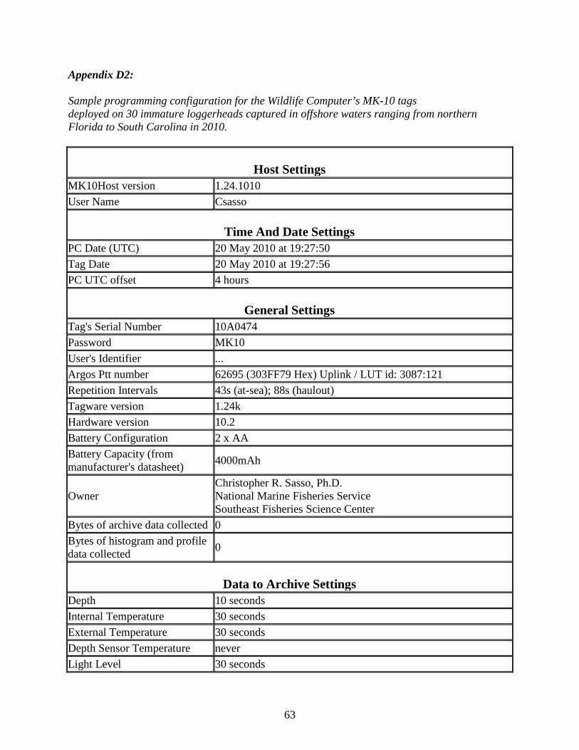
Appendix D: Southern sea turtle tagging study, summer 2010: Southeast Fisheries Science Center Katie Mansfield Southeast Fisheries Science Center, 75 Virginia Beach Drive, Miami, FL 33149 Background The Atlantic Marine Assessment Program for Protected Species project (AMAPPS) is part of a large, multi-agency initiative to provide a comprehensive assessment of marine mammal, sea turtle, and seabird abundance and spatial distribution in US waters of the western North Atlantic Ocean. The goal of this initiative is to provide seasonal, spatially-explicit density estimates of marine mammals, sea turtles, and seabirds in the western north Atlantic. Data will be collected on the seasonal distribution and abundance of these taxa using direct aerial and shipboard surveys conducted by scientists from the National Marine Fisheries Service and the US Fish and Wildlife Service. Telemetry studies, passive acoustic monitoring, and development of alternative survey methodologies are also part of AMAPPS. The telemetry data will be used to develop corrections for availability bias in the abundance survey data and to collect additional data on habitat use and life history, residence time, and frequency of use. The US Mid-Atlantic region provides important foraging, post-nesting and juvenile developmental habitat for loggerhead sea turtles. Data collection for this study is expected to occur over multiple years from 2010 to 2012. As part of the AMAPPS initiative, the Southeast Fishery Science Center (SEFCS) deployed 30 satellite tags on immature loggerhead sea turtles captured in offshore waters ranging from northern Florida to South Carolina. Methods In collaboration with the South Carolina Department of Natural Resources, 30 Wildlife Computers MK-10 satellite tags were deployed on immature loggerhead sea turtles from 24 May – 14 July 2010. Turtles were trawl-captured in coastal waters between northern Florida and North Carolina using methods described by Arendt et al. (2009). All turtles were weighed, measured and flipper tagged prior to release. Turtles were categorized as either ‘small’ (n=15) or ‘large’ (n=15) juveniles. Small turtles were <72.0 cm straight carapace length (SCL); large turtles were ≥72.0 cm SCL. Satellite tags were programmed with a 24h on, 72h off duty cycle. Twelve depth bins (0-5m, 5-10m, 10-15m, 15-20m, 20-25m, 25-30m, 30-35m, 35-40m, 40-45m, 45-50m, 50-100m and >100m) and fourteen time-at-temperature bins were programmed (in 2˚C intervals within the range 8˚ - 32˚C and >32˚C). See Appendix D2 for complete programming configuration for the Wildlife Computer MK-20 tags. Time at depth was recorded for every meter within the top five meters of the water column, followed by 10-meter bins from 10m to 50m, fifty-meter bins between 50-150m, and a final >150m bin. A dive was defined as >30 seconds in duration and >0.5 m depth.

59

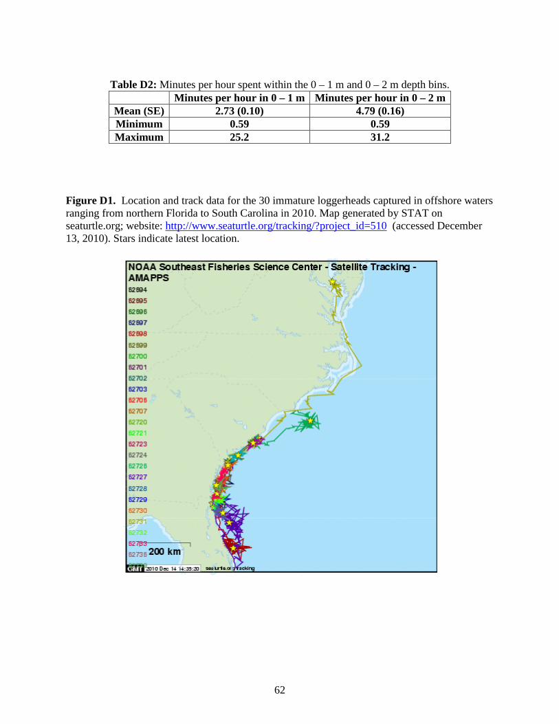
Tags were attached to the turtles’ first and second vertebral scutes using methods described by Mansfield et al. (2009), and Seney and Landry (2008). One modification to these attachment methods included the use of Powers T-308 epoxy in place of the PowerFast™ epoxy due to the unavailability of the latter. Using the ARGOS satellite data processing system, all location data derived from the tags were archived and filtered based on accuracy of transmission (ARGOS Location Codes [LC] 3-0, A and B in order of declining location accuracy; CLS 2007). Data were also filtered based on turtle behavior (reasonable swim speeds and distances between locations), and tracks were reconstructed using the Satellite Tracking and Analysis Tool (STAT; Coyne and Godley 2005). Results Average size of the loggerhead turtles satellite tagged was 70.7 cm SCL (± 6.1 SD; range: 58.1-79.8 cm SCL; Table D1). As of November 22, 2010, tags transmitted for 18 to 167+ days (averaging 92.9 d ± 41.4 d SD), where six tags were still actively transmitting (Table D1). As of 22 November 2010, 86.2% of the ARGOS location codes (LC) received from the tags were LC A (20.8%) or B (65.9%). Minutes spent from 0 – 1m and 0 – 2m are summarized in Table D2. Figure D1 shows the composite tracking map for these tags during the study period. With the exception of one animal, most turtles remained within close or regional proximity (approximately <100-300 km) to their capture location. All turtles remained on the continental shelf within near-shore coastal waters for the duration of their transmission period. One turtle immediately traveled north to Maryland’s waters of the Chesapeake Bay where it remained until its tag ceased transmitting in late August 2010. Acknowledgements The telemetry portion of this project was conducted in cooperation with the South Carolina Department of Natural Resources. We wish to thank Mike Arendt, Jeff Schwenter, Julia Byrd, their research crew, and the captains and crews of the R/Vs Lady Lisa and Georgia Bulldog for assisting with this project. Project sponsors This is a joint project between the National Oceanic and Atmospheric Administration (NOAA) National Marine Fisheries Service (NMFS) Southeast Fisheries Science Center (SEFSC) and Northeast Fisheries Science Center (NEFSC), the Bureau of Ocean Energy Management, Regulation, and Enforcement (BOEMRE; formerly the Minerals Management Service), and the US Fish and Wildlife Service (FWS). Literature cited Arendt, M, J. Byrd, A. Segars, P. Maeir, J. Schwenter, D. Burgess, J. Boynton, D. Whitaker, L.

Liguori, L. Parker, D. Owens and G. Blanvillain. 2009. Examination of Local Movement and Migratory Behavior of Sea Turtles During Spring and Summer Along the Atlantic Coast off the Southeastern United States, Final Project Report to the National Marine Fisheries Service National Oceanic and Atmospheric Administration. Final grant report for grant number NA03NMF4720281. 164 pp.

60

CLS America, Inc. 2007. ARGOS User’s manual: worldwide tracking and environmental monitoring by satellite. Argos/CLS, Toulouse, France, October 14, 2008 update. http://www.argos-system.org/manual/index.html#home.htm (accessed October 1, 2010).

Coyne, M.S., B.J. Godley. 2005. Satellite Tracking and Analysis Tool (STAT): an integrated

system for archiving, analyzing and mapping animal tracking data. MEPS 301:1-7. Mansfield, K.L., V.S. Saba, J. Keinath, and J.A. Musick. 2009. Satellite telemetry reveals a

dichotomy in migration strategies among juvenile loggerhead sea turtles in the northwest Atlantic. Marine Biology. 156:2555-2570.

Seney E.E. and A.M. Landry, Jr. 2008. Movements of Kemp’s ridley sea turtles nesting on the

upper Texas coast: implications for management. Endangered Species Research 4(1-2):73-84 (doi:10.3354/esr00077).

61

Table D1: Size (straight carapace length, SCL), release date, location, and days at large for all loggerhead sea turtles tagged in the SE tagging project. Data summarized through 11/22/2010.

Tag ID SCL (cm) Release date Release latitude

Release longitude Last location Last uplink

Days at large

62694 62.7 7/13/2010 30.562 N -81.407 W 11/19/2010 11/19/2010 129 62695 72.4 5/24/2010 30.722 N -79.767 W 7/25/2010 7/25/2010 62 62696 58.1 6/14/2010 31.522 N -81.157 W 9/8/2010 9/8/2010 86 62697 70.5 6/14/2010 31.322 N -81.157 W 8/27/2010 8/27/2010 74 62698 77.1 6/22/2010 30.533 N -81.421 W 11/19/2010 11/19/2010 50 62699 78.4 6/17/2010 32.055 N -80.699 W 9/20/2010 9/20/2010 95 62700 60.9 6/7/2010 32.753 N -79.717 W 10/14/2010 10/14/2010 129 62701 76.4 5/27/2010 32.907 N -79.490 W 9/17/2010 9/17/2010 113 62702 69.7 6/30/2010 32.000 N -80.760 W 10/29/2010 10/29/2010 121 62703 75.4 6/10/2010 30.536 N -81.381 W 6/28/2010 6/28/2010 18 62706 72.6 6/14/2010 31.320 N -81.157 W 9/2/2010 9/2/2010 80 62707 79.6 6/17/2010 31.187 N -81.114 W 7/10/2010 7/10/2010 23 62720 65.9 6/8/2010 32.745 N -79.706 W 11/22/2010 11/22/2010 167 62721 58.3 7/9/2010 31.116 N -81.285 W 10/29/2010 10/29/2010 112 62723 63.7 6/22/2010 30.533 N -81.421 W 11/22/2010 11/22/2010 153 62724 71.4 7/8/2010 31.315 N -81.159 W 8/9/2010 8/9/2010 32 62726 76.1 6/8/2010 32.802 N -79.576 W 11/19/2010 11/19/2010 164 62727 72.7 6/22/2010 30.533 N -81.421 W 10/23/2010 10/23/2010 123 62728 66.6 7/12/2010 30.673 N -81.365 W 10/11/2010 10/11/2010 91 62729 79.8 6/2/2010 31.954 N -80.727 W 7/4/2010 7/16/2010 32 62730 73.7 6/15/2010 31.331 N -81.135 W 10/23/2010 10/23/2010 130 62731 73.8 6/16/2010 32.051 N -80.747 W 8/30/2010 8/30/2010 75 62732 75.4 6/24/2010 30.705 N -81.435 W 10/20/2010 10/20/2010 118 62733 70.8 6/24/2010 30.738 N -81.425 W 11/22/2010 11/22/2010 151 62736 74.7 6/15/2010 31.244 N -81.119 W 8/6/2010 8/6/2010 52 62739 68.9 7/7/2010 31.184 N -81.215 W 9/2/2010 9/2/2010 57 62740 66.2 6/10/2010 30.535 N -81.364 W 9/20/2010 9/20/2010 102 62741 66.9 6/9/2010 32.737 N -79.651 W 8/30/2010 8/30/2010 82 62742 66.7 7/14/2010 30.618 N -81.434 W 10/11/2010 10/11/2010 89 62743 76.5 6/3/2010 32.270 N -80.410 W 8/18/2010 8/18/2010 76

62

Table D2: Minutes per hour spent within the 0 – 1 m and 0 – 2 m depth bins.

Minutes per hour in 0 – 1 m Minutes per hour in 0 – 2 m Mean (SE) 2.73 (0.10) 4.79 (0.16) Minimum 0.59 0.59 Maximum 25.2 31.2

Figure D1. Location and track data for the 30 immature loggerheads captured in offshore waters ranging from northern Florida to South Carolina in 2010. Map generated by STAT on seaturtle.org; website: http://www.seaturtle.org/tracking/?project_id=510 (accessed December 13, 2010). Stars indicate latest location.

63

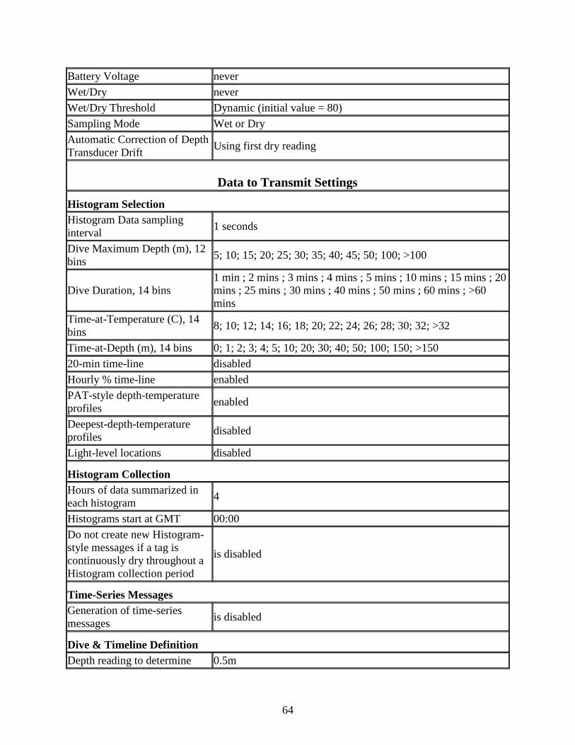
Appendix D2: Sample programming configuration for the Wildlife Computer’s MK-10 tags deployed on 30 immature loggerheads captured in offshore waters ranging from northern Florida to South Carolina in 2010.

Host Settings

MK10Host version 1.24.1010 User Name Csasso

Time And Date Settings

PC Date (UTC) 20 May 2010 at 19:27:50 Tag Date 20 May 2010 at 19:27:56 PC UTC offset 4 hours

General Settings

Tag's Serial Number 10A0474 Password MK10 User's Identifier ... Argos Ptt number 62695 (303FF79 Hex) Uplink / LUT id: 3087:121 Repetition Intervals 43s (at-sea); 88s (haulout) Tagware version 1.24k Hardware version 10.2 Battery Configuration 2 x AA Battery Capacity (from manufacturer's datasheet) 4000mAh

Owner Christopher R. Sasso, Ph.D. National Marine Fisheries Service Southeast Fisheries Science Center

Bytes of archive data collected 0 Bytes of histogram and profile data collected 0

Data to Archive Settings

Depth 10 seconds Internal Temperature 30 seconds External Temperature 30 seconds Depth Sensor Temperature never Light Level 30 seconds

64

Battery Voltage never Wet/Dry never Wet/Dry Threshold Dynamic (initial value = 80) Sampling Mode Wet or Dry Automatic Correction of Depth Transducer Drift Using first dry reading

Data to Transmit Settings

Histogram Selection Histogram Data sampling interval 1 seconds

Dive Maximum Depth (m), 12 bins 5; 10; 15; 20; 25; 30; 35; 40; 45; 50; 100; >100

Dive Duration, 14 bins 1 min ; 2 mins ; 3 mins ; 4 mins ; 5 mins ; 10 mins ; 15 mins ; 20 mins ; 25 mins ; 30 mins ; 40 mins ; 50 mins ; 60 mins ; >60 mins

Time-at-Temperature (C), 14 bins 8; 10; 12; 14; 16; 18; 20; 22; 24; 26; 28; 30; 32; >32

Time-at-Depth (m), 14 bins 0; 1; 2; 3; 4; 5; 10; 20; 30; 40; 50; 100; 150; >150 20-min time-line disabled Hourly % time-line enabled PAT-style depth-temperature profiles enabled

Deepest-depth-temperature profiles disabled

Light-level locations disabled

Histogram Collection Hours of data summarized in each histogram 4

Histograms start at GMT 00:00 Do not create new Histogram-style messages if a tag is continuously dry throughout a Histogram collection period

is disabled

Time-Series Messages Generation of time-series messages is disabled

Dive & Timeline Definition Depth reading to determine 0.5m

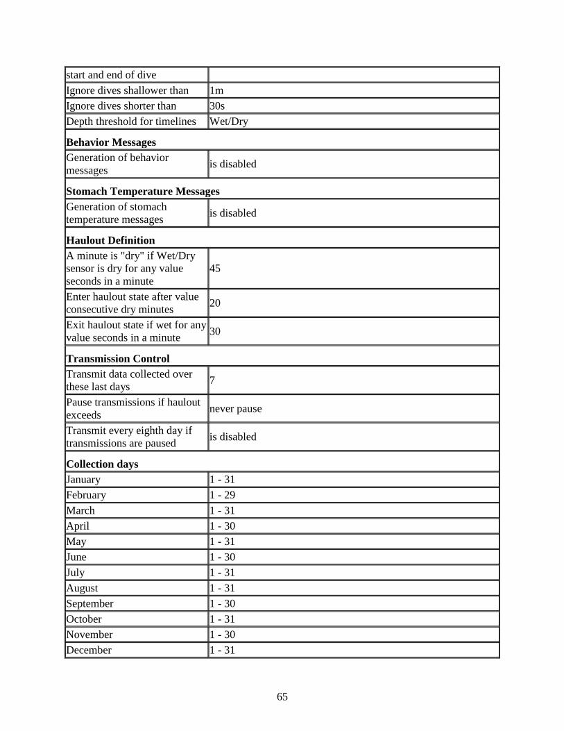
65

start and end of dive Ignore dives shallower than 1m Ignore dives shorter than 30s Depth threshold for timelines Wet/Dry

Behavior Messages Generation of behavior messages is disabled

Stomach Temperature Messages Generation of stomach temperature messages is disabled

Haulout Definition A minute is "dry" if Wet/Dry sensor is dry for any value seconds in a minute

45

Enter haulout state after value consecutive dry minutes 20

Exit haulout state if wet for any value seconds in a minute 30

Transmission Control Transmit data collected over these last days 7

Pause transmissions if haulout exceeds never pause

Transmit every eighth day if transmissions are paused is disabled

Collection days January 1 - 31 February 1 - 29 March 1 - 31 April 1 - 30 May 1 - 31 June 1 - 30 July 1 - 31 August 1 - 31 September 1 - 30 October 1 - 31 November 1 - 30 December 1 - 31

66

Relative transmit Priorities Histogram, Profiles, Time-lines, Stomach Temperature high (3 transmission(s))

Fast-GPS and Light-level Locations none (0 transmission(s))

Behavior and Time-Series none (0 transmission(s)) Status Every 20 transmissions

When to Transmit Settings

Initially transmit for these days regardless of settings below 1

Transmit hours 0 - 23

Transmit days January 3, 6, 9, 12, 15, 18, 21, 24, 27, 30 February 2, 5, 8, 11, 14, 17, 20, 23, 26 March 1, 4, 7, 10, 13, 16, 19, 22, 25, 28, 31 April 3, 6, 9, 12, 15, 18, 21, 24, 27, 30 May 3, 6, 9, 12, 15, 18, 20, 23, 26, 29 June 1, 4, 7, 10, 13, 16, 19, 22, 25, 28 July 1, 4, 7, 10, 13, 16, 19, 22, 25, 28, 31 August 3, 6, 9, 12, 15, 18, 21, 24, 27, 30 September 2, 5, 8, 11, 14, 17, 20, 23, 26, 29 October 2, 5, 8, 11, 14, 17, 20, 23, 26, 29 November 1, 4, 7, 10, 13, 16, 19, 22, 25, 28 December 1, 4, 7, 10, 13, 16, 19, 22, 25, 28, 31

Daily Transmit Allowance January 500 [Accumulate, Optimize for battery life] February 500 [Accumulate, Optimize for battery life] March 500 [Accumulate, Optimize for battery life] April 500 [Accumulate, Optimize for battery life] May 500 [Accumulate, Optimize for battery life] June 500 [Accumulate, Optimize for battery life] July 500 [Accumulate, Optimize for battery life] August 500 [Accumulate, Optimize for battery life] September 500 [Accumulate, Optimize for battery life] October 500 [Accumulate, Optimize for battery life] November 500 [Accumulate, Optimize for battery life] December 500 [Accumulate, Optimize for battery life]

67

Channel Settings

Depth Channel: 0; Range: -40m to 1000m; Resolution: 0.5m; ADaddress: 02

Internal Temperature Channel: 1; Range: -40C to 60C; Resolution: 0.05C; ADaddress: 04

External Temperature Channel: 2; Range: -40C to 60C; Resolution: 0.05C; ADaddress: 03

Depth Sensor Temperature Channel: 3; Range: -40C to 60C; Resolution: 0.05C; ADaddress: 05

Light Level Channel: 4; Range: 0 to 1024; Resolution: 0.25; ADaddress: 12

Battery Voltage Channel: 14; Range: 0V to 5V; Resolution: 0.0048V; ADaddress: 13

Wet/Dry Channel: 15; Range: 0 to 255; Resolution: 1; ADaddress: 21

68

Appendix E: Canadian Grand Banks sea turtle tagging study, 2010: Southeast Fisheries Science Center Christopher R. Sasso Southeast Fisheries Science Center, 75 Virginia Beach Drive, Miami, FL 33149 Background The staff of the Southeast Fisheries Science Center uses satellite tags to assess annual survival rates of sea turtles, determine the impact of fisheries interactions, and describe the spatial distribution of sea turtles. This work has been conducted extensively with commercial fishing fleets to access turtles and to develop satellite tagging capabilities; in particular, work is regularly conducted with longline fisherman. A pilot study to estimate pelagic juvenile loggerhead survival rates was conducted in 2003. In 2010, with AMAPPS and Stock Assessment Improvement Plan (SAIP) monies, a full study of pelagic juvenile survival has been implemented. The planned research for the summer of 2011 will determine survival rates of oceanic juveniles which will allow the National Marine Fisheries Service (NMFS) to better predict the recruitment of juvenile turtles to the neritic habitat from the oceanic habitat, where the neritic habitat is the region where the NMFS aerial surveys have observed and counted turtles. Methods During the summer of 2011, the captain of the F/V Eagle Eye II, a commercial longliner, will deploy up to 50 satellite tags on sea turtles ≥30 cm i n the Canadian Grand Banks Northeast Distant Region of the Atlantic Ocean. The search will occur on relatively calm days in warm waters (≥70˚F) and along oceanographic fronts where loggerhead turtles may congregate. Each day’s search will be at least 8 hours in duration. Once turtles are sighted, an inflatable boat will be launched with the captain (or their designee) and one crew member aboard to pursue the loggerhead turtle. Turtles will be dip netted or captured by hand from the surface, placed in the inflatable boat, and ferried to the fishing vessel where pop-off archival transmitting tags will be attached. The study will end once five (5) days of searching have been expended or up to 50 turtles ≥30 cm straight carapace length (SCL) have been captured, whichever occurs first. The tags will be programmed to pop-off after one year and then transmit their data. These data will then be analyzed to estimate survival rates for this life stage of loggerhead sea turtles. Results This study was not completed in 2010 due to weather conditions on the Grand Banks, but will resume in summer 2011. The F/V Eagle Eye II has already been contracted to capture the oceanic loggerhead turtles for this research.

69

Appendix F: Estimation of oceanic stage duration for loggerhead sea turtles, 2010: Southeast Fisheries Science Center Larisa Avens Southeast Fisheries Science Center, Beaufort Laboratory, 101 Pivers Island Rd., Beaufort, NC 28516 Background The Atlantic Marine Assessment Program for Protected Species (AMAPPS) aerial abundance surveys are conducted over waters from the US east coast to about the 100-2000m depth contours, depending on the location. These waters are considered to be part of the loggerhead turtles’ neritic life stage. However, many loggerheads are not in this life stage and thus not within the aerial survey study area. Before a loggerhead enters the neritic stage it is in the oceanic stage which is located in deeper waters within the US and in other countries territories. The objective of this project is to combine skeleto-chronological and stable isotope analyses of skeletal growth marks (GMs) in juvenile North Atlantic loggerhead sea turtle humeri to refine estimates of the duration spent in the oceanic stage. These data will allow assessment of the number of young age classes that have not yet entered the neritic stage in habitats along the east coast of the US, where the aerial abundance surveys are being conducted. This project will focus on loggerheads because this is the one species for which we have access to oceanic stage juveniles in the eastern North Atlantic and because of the continued concern over the decline in nest numbers and the potential change in Endangered Species Act (ESA) listing status from threatened to endangered. This project was funded by a combination of AMAPPS and National Marine Fisheries Service (NMFS) Stock Assessment Improvement Plan (SAIP) funds. Methods The Southeast Fisheries Science Center (SEFSC) will analyze humeri from both oceanic and neritic stage juveniles. This is necessary because analysis solely of samples obtained from oceanic stage juveniles that have not yet completed the oceanic stage would only provide a minimum estimate of the oceanic stage duration. Conversely, the humeri of most neritic juveniles, who have left the oceanic stage, exhibit skeletal growth mark (GM) resorption, where early GMs are destroyed as bone is reconstructed during growth; thus, eliminating the possibility of estimating the oceanic stage directly through GM counts of neritic stage juveniles. As a result, analysis of humeri from both oceanic and neritic stage juveniles is needed to address this question and so the project components include the following:

1) Assess the GM spacing in neritic juvenile humeri to identify the GM potentially associated with the oceanic to neritic transition;

2) Validate the proposed transition points by sub-sampling the bone in the GM spaces and analyzing the carbon and nitrogen stable isotope signatures to assess potential shifts in isotope values which are due to the change in environment and prey species when the animal transitions from the oceanic stage to the neritic stage;

3) From neritic juvenile humeri obtain GM counts, as well as diameter measurements of GMs and the resorption cores (where early GMs have already been destroyed); and

70

4) Combine data from (3) with GM counts and diameter measurements from oceanic stage juveniles to model juvenile loggerhead age and growth. This will result in the estimation of the mean, range, and variability of the oceanic stage duration.

Results To date, humeri obtained from 69 small, neritic juvenile loggerhead sea turtles stranded along the east coast of the US have been prepared for histological processing, decalcified, microtomed, and stained to highlight the skeletal GMs within the humeri. A putative transition GM was identified in each of these histologically processed sections. In addition, a non-histologically processed section from each bone was sent to Dr. Jeff Seminoff at the NMFS Southwest Fisheries Science Center (SWFSC) for stable isotope analysis. Dr. Seminoff’s laboratory is in the process of using a micro-sampler to obtain bone tissue between the GMs of each of the 69 bones. The micro-samples are currently being analyzed to assess changes in carbon and nitrogen stable isotope signatures that might serve to validate the timing of the transition relative to GM deposition. In addition to these ‘new’ 69 humeri, the SEFSC has re-processed 85 ‘old’ humerus sections that were used in an earlier study of loggerhead age and growth (Snover 2002). Stained humerus sections typically fade fairly quickly, rendering them useless for long-term analysis. However, it is possible to remove the old stain from such sections and re-stain them one additional time. This has been done for the 85 ‘old’ humeri. High-magnification, sequential, partial images were then taken of each the ‘new’ and ‘old’ sections. Then the partial images were stitched together using imaging software to yield calibrated, high-resolution digital images which can be archived. Two independent readers have worked with the calibrated digital images of all of the humeri to achieve consensus on the GM count and the location of the GM associated with the oceanic to neritic transition of these neritic juveniles. Finally, through collaborators in Portugal, we have obtained 44 humeri from oceanic stage loggerheads which were by-caught in fisheries near the island of Madeira in the eastern North Atlantic. The SEFSC has begun preparing these bones for histological processing and analysis. Acknowledgements We thank the Sea Turtle Stranding and Salvage Network for all of their efforts to collect the US neritic loggerhead sea turtle humeri used for this research. Literature cited Snover, ML. 2002. Growth and ontogeny of sea turtles using skeletochronology: methods,

validation, and application to conservation. PhD dissertation, Duke University, Durham, NC.