© 2010 by Onur Hosten. All rights reserved.

APPLICATIONS OF QUANTUM MEASUREMENT TECHNIQUES: COUNTERFACTUAL QUANTUM COMPUTATION,

SPIN HALL EFFECT OF LIGHT, AND ATOMIC‐VAPOR‐BASED PHOTON DETECTORS

BY

ONUR HOSTEN

DISSERTATION

Submitted in partial fulfillment of the requirements for the degree of Doctor of Philosophy in Physics

in the Graduate College of the University of Illinois at Urbana‐Champaign, 2010

Urbana, Illinois

Doctoral Committee:

Assistant Professor Brian L. DeMarco, Chair Professor Paul G. Kwiat, Director of Research Professor Gordon A. Baym Professor David W. Hertzog

ii

Abstract

This dissertation investigates several physical phenomena in atomic and optical physics, and quantum

information science, by utilizing various types and techniques of quantum measurements. It is the deeper

concepts of these measurements, and the way they are integrated into the seemingly unrelated topics

investigated, which binds together the research presented here. The research comprises three different

topics: Counterfactual quantum computation, the spin Hall effect of light, and ultra-high-efficiency

photon detectors based on atomic vapors.

Counterfactual computation entails obtaining answers from a quantum computer without actually

running it, and is accomplished by preparing the computer as a whole into a superposition of being

activated and not activated. The first experimental demonstration is presented, including the best

performing implementation of Grover’s quantum search algorithm to date. In addition, we develop new

counterfactual computation protocols that enable unconditional and completely deterministic operation.

These methods stimulated a debate in the literature, on the meaning of counterfactuality in quantum

processes, which we also discuss.

The spin Hall effect of light entails tiny spin-dependent displacements, unsuspected until 2004, of a

beam of light when it changes propagation direction. The first experimental demonstration of the effect

during refraction at an air-glass interface is presented, together with a novel enabling metrological tool

relying on the concepts of quantum weak measurements. Extensions of the effect to smoothly varying

media are also presented, along with utilization of a time-varying version of the weak measurement

techniques.

Our approach to ultra-high-efficiency photon detection develops and extends a recent novel

non-solid-state scheme for photo-detection based on atomic vapors. This approach is in principle capable

of resolving the number of photons in a pulse, can be extended to non-destructive detection of photons,

and most importantly is proposed to operate with single-photon detection efficiencies exceeding 99%,

ideally without dark counts. Such a detector would have tremendous implications, e.g., for optical

quantum information processing. The feasibility of operation of this approach at the desired level is

studied theoretically and several promising physical systems are investigated.

iii

To my family

iv

Acknowledgements This work was supported in part by the IARPA-funded U.S. Army Research Office Contract

No. W911NF-05-0397, NSF Grant PHY-0903865, and Harry G. Drickamer Graduate Fellowship. I am

indebted to my advisor and future collaborator Paul Kwiat for giving me the indispensible opportunity to

walk together an enthusiastic and passionate path of research, and I thank him for his continuous support

and his letting me be. I thank my family for their support and their faith in me. I thank my lab mates for

joyful times spent in the office, lab and outside of work. Finally, I thank my wife to be for the flowers, for

our misbehaved love dog ‘Fabn’, for her support, understanding, never ending interest in my research,

and her faith and respect in me.

v

Table of Contents

List of Figures ......................................................................................................................... vii

List of Abbreviations .............................................................................................................. ix

Chapter 1 Introduction ..................................................................................................... 1 1.1 Quantum measurements – Example I: Spin projection measurement ......................... 1 1.2 Quantum measurements – Example II: Weak measurements with pre- and post-

selection ....................................................................................................................... 4 1.3 Quantum measurements – Example III: Quantum interrogation ................................. 6 1.4 Quantum measurements – Example IV: Photon detection with atoms ....................... 9 1.5 Quantum measurements – Example V: Non-demolition measurements of photons . 11 1.6 Closing remarks ......................................................................................................... 12

Chapter 2 Counterfactual Quantum Computation – I: Concepts, ideas and the experiment .............................................................................................................. 14

2.1 Introduction ................................................................................................................ 14 2.2 The experiment .......................................................................................................... 16

2.2.1 Experimental encoding of the search algorithm ............................................ 18 2.2.2 Details of the experiment ............................................................................... 20

2.3 High efficiency methods ............................................................................................ 22 2.3.1 Details of the qubit-by-qubit interrogation technique .................................... 24 2.3.2 Discussion of cases involving more general algorithms ................................ 28

2.4 Other potential implementations of CFC ................................................................... 30 2.5 Error correction capabilities ...................................................................................... 31 2.6 Conclusions ................................................................................................................ 33

Chapter 3 Counterfactual Quantum Computation – II: The meaning of counterfactuality .................................................................................................... 34

3.1 Quantum histories approach ...................................................................................... 35 3.2 Weak measurements approach .................................................................................. 38

Chapter 4 Spin Hall Effect of Light – I: Sharp index variation .................................. 42 4.1 Conceptual introduction ............................................................................................. 43 4.2 Theory: Spin Hall effect of light at an interface ........................................................ 46

4.2.1 General polarization dependence of the displacements ................................. 48

vi

4.2.2 Contradicting theories and angular momentum conservation ........................ 50 4.3 Weak measurements as a metrological tool ............................................................... 54

4.3.1 The modified weak value ............................................................................... 55 4.4 The experiment .......................................................................................................... 58 4.5 Conclusions ................................................................................................................ 61

Chapter 5 Spin Hall Effect of Light – II: Smooth index variations ............................ 63 5.1 Theory: Smoothly varying index of refraction .......................................................... 63 5.2 AC weak measurements in smoothly varying media ................................................ 69

Chapter 6 Atomic-vapor-Based Ultrahigh-efficiency Photon Detectors .................... 73 6.1 Conceptual introduction ............................................................................................. 75 6.2 The read-out step ....................................................................................................... 77 6.3 Photon-atom state transfer ......................................................................................... 80

6.3.1 Direct photon absorption ................................................................................ 82 6.3.2 Stimulated photon absorption ........................................................................ 87 6.3.3 Summary of the findings ................................................................................ 93

6.4 Alternative schemes: Alkaline Earth atoms ............................................................... 93 6.4.1 Direct photon absorption in Barium ............................................................... 94 6.4.2 Working in the triplet manifold of Strontium ................................................ 97 6.4.3 Two-photon ionization scheme ...................................................................... 98

6.5 Potential extension to non-demolition detection of photons ..................................... 99 6.6 Conclusions .............................................................................................................. 101

Appendix A Supplements for Counterfactual Quantum Computation ....................... 103 A.1 A method to interrogate all database elements simultaneously ............................... 103 A.2 Liquid crystal phase retarders .................................................................................. 104 A.3 POVM measurements .............................................................................................. 106

Appendix B Supplements for Spin Hall Effect of Light ................................................ 109 B.1 Modifications due to multiple surfaces .................................................................... 109

References ............................................................................................................................. 111

vii

List of Figures Figure 1.1: An example of a quantum measurement.. ............................................................................. 2 Figure 1.2: The schematic of the weak limit of the quantum measurement shown in Figure 1.1.b,

with pre-selection (i.e., state preparation) and an additional post-selection. ........................ 5 Figure 1.3: An example of quantum interrogation with the aid of an atom-spin interferometer. ............ 7 Figure 1.4: A conceptual example of single-photon detection with an atom. ......................................... 9 Figure 2.1: Realization of CFC is as an optical interferometer. ............................................................ 16 Figure 2.2: Experimentally determined probabilities for the output state of 670-nm single photons

conditionally prepared through downconversion [38]. ....................................................... 17 Figure 2.3: The schematic of the optical circuit realizing the search algorithm in a database of four

elements. ............................................................................................................................. 19 Figure 2.4: The optical circuit used for the CFC experiment. ............................................................... 21 Figure 2.5: Proposed set-up for the ‘chained Zeno effect’. ................................................................... 23 Figure 2.6: The quantum circuit diagram of the high-efficiency qubit-by-qubit-interrogation

technique. ........................................................................................................................... 25 Figure 3.1: A simplified setup summarizing the controversial aspect of CFC. ..................................... 35 Figure 3.2: Decomposition of the dynamical evolution of CFC into histories (or paths) for the case

of the nested interferometer example. ................................................................................ 37 Figure 4.1: The spin Hall effect of light at an air-glass interface. ......................................................... 44 Figure 4.2: Illustration of the two different polarization models. .......................................................... 51 Figure 4.3: Comparison of different theories. ........................................................................................ 53 Figure 4.4: A weak quantum measurement with PPS. ........................................................................... 55 Figure 4.5: Experimental setup for characterizing the spin Hall effect of light. .................................... 59 Figure 4.6: Experimental results for the magnitude of the opposite shifts of the two spin

components as a function of incidence angle. .................................................................... 60 Figure 5.1: Pictorial representation of defining a new polarization basis set that depends on the

local propagation direction. ................................................................................................ 66 Figure 5.2: The expected SHEL displacements for a beam of light propagating through a region

with a gradient in the refractive index. ............................................................................... 69 Figure 5.3: Experimental setup using an AC post-selection technique for observing the SHEL in a

medium with smoothly varying index of refraction. .......................................................... 70 Figure 6.1: An example of a possible atomic-vapor based photon detector with alkali atoms

(particularly Rubidium). ..................................................................................................... 76 Figure 6.2: Illustration of a non-perfect read-out mechanism. .............................................................. 78 Figure 6.3: Absorption of a single photon by an atom in free space. .................................................... 81 Figure 6.4: Illustration of the time dependent absorption probabilities for the direct photon

absorption scheme for a single Barium atom. .................................................................... 86 Figure 6.5: Illustration of the time dependent absorption probabilities for the stimulated photon

absorption scheme for a single Rubidium atom. ................................................................ 90

viii

Figure 6.6: Photon detection in a Barium vapor via direct photon absorption. ..................................... 95 Figure 6.7: Photon detection in the triplet manifold of 88Sr via TPRT. ................................................. 98 Figure A.1: Optical schematic of the method to interrogate all database elements simultaneously. ... 104 Figure A.2: Phase retardence (phi) at 632.8 nm of the liquid crystal pixels for the polarization

component along the optic axis, as a function of the applied RMS voltage. .................... 105

ix

List of Abbreviations

AC Alternating current

APD Avalanche photodiode

BBO Beta barium borate

BS Beam splitter

CCW Counter-clockwise

CEM Channel electron multiplier

CFC Counterfactual computation

CW Clockwise

DC Direct current

DOF Degree of freedom

EIT Electromagnetically induced transparency

FORT Far-off resonance optical dipole trap

GSA Grover’s search algorithm

H Horizontal

HWP Half-wave plate

L Left circular

LC Liquid crystal

LP Linear polarizer

ME Marked element

MOT Magneto-optical trap

PBS Polarizing beam splitter

PC Pockels cell

PMT Photo-multiplier tube

x

PNR Photon-number resolution

POVM Positive operator-valued measure

PPS Pre- and post-select(tion/ed)

PS Position sensor

QI Quantum information

QND Quantum non-demolition R Right circular

RWA Rotating wave approximation

SHEL Spin Hall effect of light

SHO Simple harmonic oscillator

SNR Signal to noise ratio

TES Transition-edge sensor

TPRT Two-photon Raman transition

V Vertical

VAP Variable angle prism

VLPC Visible light photon counters

WH Walsh-Hadamard

XPM Cross-phase modulation

1

Chapter 1 Introduction

This dissertation will investigate several physical phenomena in atomic and optical physics, and quantum

information science, by utilizing various techniques of quantum measurements. Indeed, several wholly

different measurement paradigms are explored, each optimized for a specific application. It is the deeper

concepts of these measurements, and the way they are integrated into the seemingly unrelated topics

investigated, which bind together the research presented here.

Three main research topics will be covered: Counterfactual quantum computation, the spin Hall effect

of light, and ultrahigh-efficiency photon detectors based on atomic vapors. The current chapter will

introduce some preliminaries about quantum measurements, and hint on their roles played in the

subsequent chapters. Chapter 2 will describe the first experimental demonstration of counterfactual

quantum computation (including the best-performing implementation of a quantum search algorithm to

date) and the development of new counterfactual protocols. Chapter 3 will cover the debates on the

meaning of counterfactuality that arose from the developed protocols. Chapter 4 will describe the first

verification of the spin Hall effect of light (at an interface between two media), along with the so-called

‘weak measurement’ techniques that enabled the experiment. Chapter 5 will explain the spin Hall effect

of light in a medium with smoothly varying index of refraction, together with an experiment utilizing a

time-varying version of the weak measurement techniques. Finally, Chapter 6 will investigate the topic of

photon detectors based on atomic vapors, aiming to understand the feasibility of an implementation and to

identify promising physical systems.

In the rest of this chapter, we will look at five seemingly different types of quantum measurements,

with five examples in the next five sections.

1.1 Quantum measurements – Example I: Spin projection

measurement

An elementary example of a quantum measurement is the determination of a spin component of an

electron (or a neutral atom possessing a net spin, e.g., the famous Stern-Gerlach spin projection

measurement with a beam of Ag atoms from an oven [1,2]). Consider an atom with a single valence

2

electron1 traversing a region of space with an inhomogeneous magnetic field that is predominantly

oriented along the z-axis, as shown in Figure 1.1.a; along the path of the beam the field is expressible to

lowest order as 0 ˆ(1 )B zε= −B z , where ε depends on the geometry. The corresponding Hamiltonian is

approximately 2 2

0 02 2ˆ ˆˆ ˆ ˆ' ' 'z z

z zp pm mH g g S B g B S zε= − ⋅ = − +S B , with 2

ˆ =S σ being the spin operator,

2ˆ

z zS σ= its third component2 (with eigenstates |↑z⟩ and |↓z⟩ and corresponding eigenvalues / 2+ and

/ 2− ), and g′ is a constant (g′ = e / me c , e < 0 for this example). The measurement interaction is the last

term ˆI zH gS z= − , with the interaction strength 0'g g Bε= − (the redundant minus signs are for future

convenience with the Heisenberg equations of motions).

1 Alkali atoms or the alkali-like atoms (Cu, Ag, Au) are examples of this. All the electrons but the outermost one

pair up to give a net spin of zero. Note that almost all of these atoms also possess nuclear spin, however, the magnetic moment due to the nuclear spin is very small in comparison to the magnetic moment of the electron spin. Consequently, we will ignore the nuclear spins since they will not play an important role in the examples that we will be describing. We could have just used an electron, but we wanted to avoid the Lorentz force.

2 The three Pauli matrices are 1

0 11 0xσ σ

⎛ ⎞≡ = ⎜ ⎟

⎝ ⎠, 2

00y

ii

σ σ−⎛ ⎞

≡ = ⎜ ⎟⎝ ⎠

, and 3

1 00 1zσ σ

⎛ ⎞≡ = ⎜ ⎟−⎝ ⎠

.

Figure 1.1: An example of a quantum measurement. a, Schematic for the measurement of the projectionof the spin of a single-valence-electron atom along the z-axis. b, A general schematic of a strong quantummeasurement of an observable A of a quantum ‘system’ with discrete eigenstates |an⟩ and correspondingeigenvalues an. The ‘meter’ is a different continuous variable quantum system (e.g., position ormomentum of a particle). The ‘system’ and the ‘meter’ interact, resulting in a joint (entangled) state inwhich different eigenstates of the observable A are correlated with different states of the ‘meter’. A finalread-out on the meter reveals information about the ‘system’. The displacements in the principalcoordinate of the meter are proportional to the eigenvalues of the associated eigenstates. For a time-

varying measurement interaction strength g(t), the proportionality constant G is given by 0

' ( ')t

tG dt g t= ∫ .

3

For this configuration, the ‘system’ observable being measured is the z- component of the spin

projection of the incoming atoms (i.e., ˆzS ), and the measuring device (the ‘meter’) is the z-component of

the linear motional degree of freedom (DOF) of the atoms. Note that the interaction Hamiltonian HI

couples the observable ˆzS to the position of the ‘meter’ (i.e., z). It is easy to see through the Heisenberg

equation of motion, 1 12

ˆˆ ˆ[ , ]z z I zit p p H g σ∂∂ = = , that this interaction Hamiltonian generates a translation in

the momentum of the ‘meter’. In particular, after the interaction, the change in the momentum of the

‘meter’ is proportional to the eigenvalue of the measured observable. We shall call the observable

conjugate to the one that appears in the interaction Hamiltonian (here the momentum along the z-

direction), the principal observable of the ‘meter’. Similarly, we shall call the observable of the ‘meter’

that appears in the interaction Hamiltonian (here the position along the z-direction), the conjugate

observable of the ‘meter’. If the measurement strength is sufficiently large (such that the involved

changes in the momentum are greater than the initial uncertainty on the momentum wave-packet), the

eigenstates of the observable can be resolved (see Figure 1.1.b).

Notice that the information about the measurement outcome is encoded on a different DOF of the

same particle (this does not have to be the case; examples where the ‘meter’ is a separate entity will be

discussed in Sections 1.4 and 1.5 in the context of destructive and non-destructive detection of photons).

Different eigenstates of the ‘system’ are now correlated with different momentum wave-packets of the

‘meter’. In particular, if the initial ‘system’ state is in a coherent superposition of multiple eigenstates of

the observable, the final state after the measurement interaction is a joint state of the ‘system’ and the

‘meter’, where the coherent superposition – an entangled state – is between ‘system’ eigenstates

correlated with different ‘meter’ momenta. Nevertheless there is no longer coherence between the system

eigenstates alone (which can be viewed as decoherence, which becomes more interesting if the meter is a

separate particle). A final read-out on the meter at this stage will collapse it into a particular momentum

wave-packet state revealing the eigenstate (and its eigenvalue)3. The subtlety is that the read-out actually

is yet another quantum measurement interaction, with the ‘meter’ being a different physical particle (or

system of particles) this time, creating a joint quantum state (in general an entangled state). Thus, there is

never a true collapse; as in the many-worlds interpretation4, the experimenter becomes entangled with the

outcomes, and in each branch of the entangled state he/she observes a particular outcome, creating the

3 For the example investigated here, the probability of collapsing into a particular momentum wave-packet is

given by the absolute square of the initial amplitude of the eigenstate correlated with the particular wave-packet (assuming a normalized state).

4 For a good review on the appearance of the classical world within quantum mechanics, see reference 131.

4

apparent experience of a collapse. Or perhaps, there is indeed a collapse when some unknown physics

takes over [3].

1.2 Quantum measurements – Example II: Weak measurements with

pre­ and post­selection

In the standard measurement paradigm (Figure 1.1.b), as the measurement strength becomes smaller

(‘weak’), the wave-packets corresponding to different eigenstates after the measurement interaction start

overlapping, preventing extraction of information in a single shot. Nevertheless, many repeated weak

measurements on a single quantum system can be equivalent to a strong measurement. Alternatively,

repeated weak measurements on identically prepared systems can allow expectation values of observables

to be extracted, and even a full reconstruction of the quantum state by measuring different observables.

Surprisingly, the reconstruction of the quantum state (i.e., measurement of the wavefunction) of a single

quantum system is also possible, but only in special circumstances, with the aid of the so-called

‘protective measurements’ [4] which utilize repeated combinations of weak and strong measurements. A

modern discussion of the current general understanding and limits of quantum measurements as they

apply to single quantum systems, in connection with achievable experiments, can be found in reference 4.

Nevertheless, most interestingly, weak measurements take on a new life when combined with pre- and

post-selection (PPS).In quantum mechanics, one is usually concerned with the probabilities of certain

measurement outcomes or with the eigenvalues, averages or variances of observables. What actually

‘happened’ between two measurements (i.e., between a PPS) is often an ill-defined question due to the

uncertainty principle. Any precise measurement to ascertain the intermediate value of an observable

between two strong measurements will disturb the state if the intermediate measurement is not made in

the same basis as the final measurement (or the initial preparation). Therefore, a strong measurement in

general will alter what happened during the intermediate interval. However, one can imagine doing very

weak measurements, at the expense of having to repeat the measurements many times (to extract

meaningful information) while disturbing the state minimally [5]. In the context of counterfactual

quantum computation (Section 3.2) we will take precisely this kind of an approach to investigate whether

a computer runs or not in obtaining an answer to a computation. The physical discussion will be on

whether or not a photon can be said to take a particular path out of a complicated interferometer.

A weak measurement with PPS (see Figure 1.2) is basically a conditional weak measurement of a

‘system’ that is initially in state |ψ1⟩. Specifically, one reads out the ‘meter’ only if the state of the

‘system’ is found to be in state |ψ2⟩ after a following strong measurement (i.e., the post-selection). Note

that the final strong measurement that would potentially result in state |ψ2⟩ of the ‘system’ is in general in

5

a different basis (i.e., different observables) than the preceding weak measurement. Conceptually, the

most important outcome of the approach is defining a new concept called the ‘weak-value’ of a quantum

variable [5]. The weak-value is a physical property of a quantum system belonging to a PPS ensemble,

and the weak-value manifests itself in the state of the ‘meter’. Specifically, given a successful post-

selection, the weak-value is a shift in the central location of the principal observable of the ‘meter’

(assuming the weak-value is real). However, as a consequence of a subtle interference effect, the central

position of the ‘meter’ can shift to exotic values that are not even bounded by the eigenvalues of the

observable (to be more precise, G times the eigenvalue, according to Figure 1.2). One can even obtain

negative weak-values for positive-definite observables, as we will see in Section 3.2.

As will be derived in Section 4.3.1, the weak-value Aw of an observable A is given by

2 1w

2 1

ˆ| ||

A ψ ψψ ψ

⟨ ⟩=

⟨ ⟩A . 1.1

Here |ψ1⟩ and |ψ2⟩ are the pre- and post-selected states respectively. The only difference from a regular

expectation value is the presence of ⟨ψ2| in place of ⟨ψ1|. Note that due to the weakness of the

measurements, the weak-values of two non-commuting observables can be measured simultaneously. As

Figure 1.2: The schematic of the weak limit of the quantum measurement shown in Figure 1.1.b, withpre-selection (i.e., state preparation) and an additional post-selection. The ‘system’ starts in the initialstate |ψ1⟩, which is in general a superposition of the eigenstates of the observable A .The ‘system’ and the‘meter’ interact, resulting in a joint state where different eigenstates of A are correlated with differentstates of the ‘meter’. However, the associated meter states overlap to a large extent. A post-selectionon the ‘system’ gives rise to interference between the ‘meter’ wave-packets that were correlated withdifferent eigenstates. When the post-selection is successful, the ‘meter’ is left in a new state with thecenter of the wave-packet in the principal observable pointing to a new value. The new value is theweak-value Aw (at least when Aw is real). Note also that the new ‘system’ state associated with themeasured ‘meter’ wave-packet is the post-selected state |ψ2⟩.

6

evident from Equation 1.1, weak-values can take on imaginary values as well as real values. When purely

imaginary values are the result, the shift in the ‘meter’ occurs in the conjugate observable (i.e., the one

that appears in the interaction Hamiltonian), as will be discussed thoroughly in Section 4.3. Note that for

the spin projection measurement of Figure 1.1.a, the principal observable is the z-momentum, and the

conjugate observable is the z-position.

Notice that the denominator of Equation 1.1 approaches zero as the PPSs approach being orthogonal to

each other, yielding potentially very large values of Aw. Thus, the smaller the likelihood of a successful

post-selection, the greater the strangeness of the values one can obtain. For example, the result of a

measurement of a component of the spin of a spin-1/2 particle (where the largest eigenvalue is / 2 , just

like the one discussed in connection to Figure 1.1.a) can turn out to be 100 [6]. In Chapter 4, we will

utilize this ‘amplification effect’ in conjunction with using purely imaginary weak-values, to enable a

novel enhancement technique that provides a tremendous increase in the signal-to-noise ratio (SNR) for

realistic experimental configurations. In particular, we will enhance the tiny spin-dependent

displacements due to the Spin Hall effect of light, allowing us to demonstrate the effect for the first time.

Further, in Chapter 5 we will use a time-varying version of the ‘amplification effect’ to achieve even

better SNRs.

A few of the other interesting examples in the literature, where weak measurements with PPS are

utilized include: how to measure negative kinetic energies [7], the ‘three-box problem’ (which is quite

similar to the problem we will investigate in Section 3.2), in which a particle is measured to be at more

than one place at once [8], Hardy’s Paradox [9], etc. Note also that even though here we used a

continuous variable ‘meter’, this need not be the case; measurements of weak-values can also be

performed with a two-level ‘meter’, i.e., a so-called qubit meter [10].

1.3 Quantum measurements – Example III: Quantum interrogation

Quantum interrogation was first introduced by Elitzur and Vaidman under the name ‘quantum-mechanical

interaction-free measurements’, since in their protocol, the presence of an object was measured without

any incident photons being scattering, or absorbed, or transmitted by the object. In the original example,

the object was a bomb that can be triggered by a single photon. The goal was to determine whether or not

the bomb was defective, i.e., if it would really explode when a single photon hits it, but without a photon

actually setting it off, so that it will work in the future when needed [11]. The name ‘interaction-free

measurements’ encountered some resistance in the scientific community, and evolved into ‘quantum

interrogation’ [12] (to include cases of partially transmissive objects)).

7

We will illustrate the idea with an atom-spin interferometer, where the setup in Figure 1.1.a functions

as a spin-dependent beam-splitter (BS), and also as a mirror for the incoming particles. The configuration

is shown in Figure 1.3. An incident particle is prepared in the spin up eigenstate of the x-projection of the

spin. Note that spin up in x-direction ( |→⟩ ) can be written in terms of the spin up/down states in the z-

direction ( | / ⟩↑ ↓ ) as 12

| (| | →⟩ = ⟩+ ⟩)↑ ↓ . After the first BS, the particle is in an equal coherent

superposition of taking the upper and lower paths, with the corresponding respective internal states | ⟩↑

and | ⟩↓ . After reflecting from the mirrors, the two paths recombine coherently, resulting in an

interference of the internal states. In the absence of an object (Figure 1.3.a), assuming that the path

lengths are adjusted properly, the internal states can be added with the same relative phase, and the final

state of the spin is again |→⟩ . Therefore, a consequent strong measurement of the spin projection along

the x-axis cannot yield the spin down result |←⟩ . On the other hand, when there is an object blocking the

lower path of the interferometer (Figure 1.3.b), no amplitude from that path can make it to the second BS

to give rise to interference; hence, the final state of the spin (provided that the particle took the upper

Figure 1.3: An example of quantum interrogation with the aid of an atom-spin interferometer. Shown aretwo cases: a, when there is no object in the interferometer, and b, when there is an object in one arm ofthe interferometer. The regions with magnetic-field B gradients (as in Figure 1.1.a) act as spin-dependentBSs and mirrors. The states | / ⟩↑ ↓ represent the up / down states of the z-component of the spin, andstates | /→ ←⟩ represent the up / down states of the x-component of the spin. The devices labeled ‘spin-xmeasurement’ perform a measurement of the spin projection along the x-axis.

8

interferometer path) is 12

| (| | )⟩ = →⟩+ ←⟩↑ . This time, there is a chance that a subsequent strong

measurement of the spin projection along the x-axis can yield the spin down result |←⟩ . In particular, this

happens overall 1/4 of the time. When it happens, we know that there was an object in the interferometer,

since there was no chance of detecting the state |←⟩ when there was no object. But most surprisingly, we

deduce the presence of the object seemingly without the particle interacting with the object, since if it had

interacted, it could not have made it to the final measurement apparatus5.

Quantum interrogation in its simple form as presented has been realized experimentally in optical

interferometers with single-photon states [13] and attenuated classical light [14], as well as in neutron

interferometry [15]. Even though the simple version presented in this section works overall 1/4 of the

time, using the concepts of the quantum Zeno effect6, quantum interrogation can be made to work with

probabilities tending to unity, as has been shown experimentally [12]. These ideas can be utilized in

practical applications, e.g., where objects to be imaged are light sensitive, and low level exposures are

desirable. An example demonstration is the imaging of a photographic film itself with reduced exposure

[16].

In Chapter 2 we will begin exploring quantum interrogation of a prototype quantum computer, and

hence be able to obtain answers from the quantum computer without actually ‘running’ it. We will present

the first experimental demonstration of this phenomenon, known as counterfactual quantum computation,

and will further analyze the use of the Zeno effect as well as a novel version of it (the chained Zeno

effect) to achieve an unconditionally successful interrogation. The resulting circumstances will create a

plethora of interesting discussions, which we address in Chapter 3.

5 Extension to the bomb-testing idea would involve replacing the object with a device that would register the

passage of the particle with an interaction that will change an internal quantum state of the device (which will in turn activate the bomb), but otherwise leave the particle state/propagation unchanged. If the activation mechanism is defective, and the interaction does not change the internal state of the device, the situation is identical to there being no object on the path. However, if the activation mechanism works correctly, the particle going through the lower path will become correlated with a different internal state of the bomb (i.e., an entanglement between the bomb and the particle). Thus, even though the amplitude from the lower path makes it to the second BS, there will be no interference in the internal spin state of the particle, since the states coming from the lower and upper arms are entangled with the states describing the bomb being activated and not being activated, respectively. Hence, the situation is effectively identical to there being an object on the path. As a consequence, on average 1/4 of the time we can assert that the bomb works fine without detonating it.

6 The Zeno effect states that in certain circumstances the time evolution of a quantum system can be slowed down with frequent measurements on the system. We will explore this phenomenon in more detail in Section 2.3.

9

1.4 Quantum measurements – Example IV: Photon detection with

atoms

Detection of a particle itself, as opposed to an observable of the particle, can be understood in the same

framework that we have been using, provided that the ‘meter’ is a physically separate quantum particle or

system, and more crucially, provided that the particle is not destroyed in the process. Measurements

satisfying these criteria will be discussed in the next section. If the particle is destroyed in the process of

Figure 1.4: A conceptual example of single-photon detection with an atom. a, An atom possessing fourenergy levels is placed inside of an ideal optical cavity. The label |g⟩ (|s⟩, |i⟩, |e⟩) corresponds to theground (metastable, intermediate, excited) state. The signal mode supported by the cavity couples to the|g⟩ to |i⟩ transition of the atom. We allow for only zero or one photons in the signal mode for this example.b, The initialization step: Any amplitude in state |s⟩ is optically pumped to state |g⟩ with the aid of the‘pump laser’ and the following spontaneous emission. Note that the atom can also decay back to state |s⟩,but with repeated trials, eventually the atom with decay to state |g⟩. c, The step for the controlledabsorption of the photon (or state transfer): When the strong ‘coupling’ laser is turned on for a finiteduration, if there is a photon in the signal mode, the system can be coherently driven to the state |s⟩ via atwo-photon Raman transition, with the photon absorbed in the process. The signal mode is sufficientlydetuned from the |g⟩ to |i⟩ transition, so that in the absence of the ‘coupling laser’ the atom essentiallyremains in state |g⟩ even if there is a photon in the signal mode. The spontaneous decay to |g⟩ or |s⟩ isnegligible since the amplitude in |i⟩ is very small throughout the process. d, The read-out step: The ‘read-out laser’ couples the |s⟩ to |e⟩ cycling transition, in which the spontaneous decay can only be to state |s⟩.Thus if the atom is in state |s⟩, it repeatedly emits photons (i.e., it fluoresces); some fraction of these canbe efficiently detected with a traditional photon detector, e.g., a photomultiplier tube or an avalanchephotodiode.

10

the measurement, some additions to our descriptions are required. First of all, we have to think in terms of

the second quantization framework of quantum mechanics, in which particles are allowed to be created or

destroyed. Here, we will consider photo-detection; however, we will not describe the standard

photoelectric-detection theory (which can be found in Chapter 14 of reference 17), but instead focus on a

different idea – photo-detection via atomic vapors [18,19].

Here we illustrate the idea in its simplest form, with a single four-level atom interacting with a single

mode of the radiation field (the ‘signal’ mode), as depicted in Figure 1.4.a. The task is to measure whether

there is a photon in the signal mode. The atom starts in state |g⟩, which is ensured by the initialization step

shown in Figure 1.4.b. Note that the initial state of the signal mode can be an arbitrary superposition of

zero- and one-photon states (i.e., the combined initial state is ( )initial| | | 0 |1g α βΨ ⟩ = ⟩ ⟩ + ⟩⊗ , with α and β

being complex amplitudes satisfying |α|2 + |β|2 = 1).

The strategy would be to first map the photon number information onto atomic state information, and

then to measure the state of the atom. By construction, the signal mode causes transitions only between

the atomic levels |g⟩ and |i⟩, the ‘coupling laser’ causes transitions only between the atomic levels |s⟩ and

|i⟩, and the ‘read-out laser’ causes transitions only between the atomic levels |s⟩ and |e⟩. The mapping is

done via the two-photon Raman transition shown in Figure 1.4.c. The effective interaction Hamiltonian

(obtained by adiabatic elimination of state |i⟩) is given by the Jaynes-Cummings Hamiltonian

( ) ( )†( ) ( ) | ,0 ,1| | ,1 ,0 |IH g t a a g t i g g iσ σ+ −= − + = − ⟩⟨ + ⟩⟨ , where †a and a are the creation and

annihilation operators for the signal mode, and, σ+ and σ− are the raising and lowering operators for the

atom between states |g⟩ and |s⟩. The right-hand side of the equation explicitly assumes the zero- and one-

photon sub-space of the Hamiltonian. When the ‘coupling laser’ is on, g(t) = g0, and when it is off,

g(t) = 0. As long as the ‘coupling laser’ is on, the time evolution is given by

( ) ( )initial 0 0exp / | | ,0 cos( ) | ,1 sin( ) | ,0IiH t g g t g i g t sα β− Ψ ⟩ = ⟩ + ⟩ + ⟩ ; when the ‘coupling laser’ is turned

off at time t = π / 2g0, the state becomes ( )final| | | | 0g i sα βΨ ⟩ = ⟩ + ⟩ ⊗ ⟩ . So far, the internal state of an

effectively two-level atom acted as the ‘meter’ to measure the occupation number observable of the

‘system’ (i.e., the signal-field mode).

The final step of the protocol is to measure the atomic state with fluorescence detection, as shown in

Figure 1.4.d. This time the ‘system’ observable is the internal state of the atom, and the ‘meter’ is the

field mode associated with spontaneous emission from the |e⟩ to |s⟩ transition of the atom (we will see the

associated interaction Hamiltonian in Section 6.3). In particular, if the atomic state is |s⟩ there will be a

stream of single photons emitted from the atom (i.e., fluorescence); these photons can then be partially

11

collected and detected with conventional single-photon detectors, as shown in Figure 1.4.a. On the other

hand, if the atomic state is |g⟩, there will be no fluorescence.

In conclusion, the overall detection method converts a single photon in the signal mode into many

photons scattered into all directions in space; these photons can be detected with a conventional

solid-state based detector. Note that the single-photon detection efficiency of the conventional detector

need not be high (since there are many fluorescence photons) in order to achieve high-efficiency detection

of the photon in the signal mode. The scheme described above forms the basis of the proposals that we

will discuss in Chapter 6, in which we investigate more realistically the feasibility of using atomic vapors

in free space to detect photons with efficiencies exceeding 99%.

1.5 Quantum measurements – Example V: Non­demolition

measurements of photons

It is known that the performance of linear optics quantum computing gates can be improved by using a

hybrid approach that combines linear-optics techniques with small amounts of nonlinearity. For example,

Kerr optical nonlinearities leading to cross-phase modulation (XPM) between two photons is extremely

weak for common materials, so a single-photon-induced π-phase shift required for photon-photon

two-qubit gates is not achievable [20]. However, the use of a strong classical probe beam (in a coherent

state |α⟩ [21]) interacting individually with the two photons, in conjunction with the measurements of its

phase, could enable deterministic two-photon gates in the optical domain by effectively amplifying the

weak nonlinearities [22,23]. The interaction leading to this particular protocol is in fact a quantum non-

demolition (QND) measurement of the photon number, which enables photons to be measured without

being absorbed, in contrast to any common light detector. To date, such a QND measurement has only

been realized with microwave photons inside of ultra-high finesse cavities in the context of cavity

quantum electrodynamics with Rydberg atoms [24,25], and also with superconducting circuits [26].

The interaction Hamiltonian for XPM is † †I s s p pH ga a a a= − where †

sa and sa are the creation and

annihilation operators for the signal mode, and, †sa and sa are the corresponding operators for the probe

mode. In terms of a quantum measurement, we can take the ‘system’ observable to be the photon number

operator †ˆs s sn a a= in the signal mode. The conjugate ‘meter’ operator that appears in the interaction

12

Hamiltonian † 2 212 ( 1)p p p pa a X Y= + − is the free Hamiltonian of the probe mode7 up to an additive constant

(in fact, this is the Hamiltonian corresponding to a simple harmonic oscillator (SHO)). The principle

‘meter’ observable should then be the time, i.e., temporal shifts (or time translation) in the ‘meter’ state.

Note that for a SHO initially in a coherent state and evolving under its free Hamiltonian, a time

translation is simply a phase shift in its complex amplitude. The consequences of the interaction will most

easily be understood in the Schrödinger picture, by time evolving an initial state8 initial| | |p s snαΨ ⟩ = ⟩ ⟩ with

the interaction Hamiltonian: ( )final initial| exp / | | |sinI p s siH t e nφαΨ ⟩ = − Ψ ⟩ = ⟩ ⟩ , with φ = gt. We see that the

phase of the coherent state in the probe mode is proportional to the number of photons in the signal

mode 9 . The overlap between two coherent states with a relative phase shift 1φ is given by

( )2 2 2| | | exp | |si ne φα α α φ⟨ ⟩ ≅ − . Thus, provided that the amplitude α of the coherent state is large enough,

the ‘meter’ states associated with different photon numbers in the signal mode can be distinguished, at

least in principle. The phase of the probe mode can then be measured (e.g., by a homodyne measurement,

where the probe beam is interfered with a reference beam, converting the phase information into intensity

information, which in turn is read by a photodiode), and the photon number in the signal mode can be

inferred without destroying the photons.

We will discuss a possible realization of non-demolition photon measurements in Section 6.5, as an

extension of the atomic-vapor-based photon detectors studied in Chapter 6.

1.6 Closing remarks

The educational and intellectual benefits of the research presented in this dissertation are, we believe,

two-fold. First, in going beyond the abstract concept of a measurement in quantum mechanics, we

investigated the detailed processes involved in performing a measurement on a quantum system.

Importantly, we have seen that quantum measurements in practice are actually equivalent to dynamical

7 †1

2( )pX a a= + and †

2( )i

pY a a= − are the quadrature operators, which are in spirit equivalent to

dimensionless position and momentum operators, and to dimensionless electric- and magnetic-field operators of a single field mode. Note that †[ , ] 1a a = implies [ , ]p pX Y i= .

8 This state means that there are ns photons in the signal mode and a coherent state with complex amplitude α in the probe mode. Note that a coherent state is a minimal uncertainty wave-packet whose probability distribution is oscillating harmonically in either quadrature (Xp or Yp) space, with constant width. Expressed in the photon-number

basis, a coherent state with complex amplitude α reads: 2| | /2

0| |

!

n

ne n

nα αα

∞−

=

⟩ = ⟩∑ .

9 If the signal mode were to be in a superposition of number states, an entangled state between the ‘system’ and the meter’ would result.

13

evolution of joint quantum systems under the Schrödinger equation. We have investigated different types

of measurements, and in what forms and circumstances they may appear in various areas of physics. We

have shown that many of the measurement types are interrelated. For example, the weak interactions

(which would lead to weak measurements) between individual photons and atoms were explored as a

means to realize a very efficient (strongly measuring) photon detector, with an eye toward eventual QND

detection, that detects the photons without destroying them. A connection between dynamic evolution and

strong measurements was revealed when we studied high-efficiency quantum interrogation

measurements, in which repeated strong measurements on part of a system resulted in a nearly unitary

evolution of the system with a continuous reduction of the wavefunction. In some circumstances, we have

seen that the way that one type of measurement operates could be illuminated by another type of

measurement: we investigated an example of this when we probed the operation of quantum interrogation

with the help of weak measurements to determine if a protocol was really counterfactual. In other

circumstances, we have seen that the operation of one type of measurement was modified by another

type: we investigated an example of this when we applied pre- and post-selection (which are basically

strong measurements) in conjunction with weak measurements to enhance the results given by the weak

measurements, which in turn were used to make ultra-precise measurements.

The second benefit was that we had the opportunity to investigate many different topics in the fields of

optics, quantum optics, quantum information science, and atomic physics, and even to measure previously

unobserved physical effects, in addition to developing new metrological tools and technologies. The

general conclusions pertaining to the different topics studied can be found at the end of respective

chapters together with the remaining questions and future directions.

14

Chapter 2 Counterfactual Quantum Computation – I: Concepts, ideas and the experiment10

What would it mean to get an answer from a quantum computer without running the computer? Let alone

the answer to this question, the question itself is even counterintuitive. However, the laws of quantum

mechanics allow us to ask such questions. The idea of so-called counterfactual quantum computation

(CFC) was put forward first in 1998 [27], and this chapter will present the first experimental

demonstration [28,29]. The strategy of measuring the information contained in a quantum computer (or in

any region of space-time), without running the computer (or without entering into the space-time region

of interest) constitutes a particular type of measurement which can be named a counterfactual

measurement. In principle, this measurement involves an inference made about a physical observable

without an actual direct measurement of it, e.g., by utilizing the absence of a result.

In fact, CFC is a logical extension of the techniques of quantum interrogation, introduced in Section

1.3, where one can detect the presence of, or even image, an object without any photons at all scattering

from, or absorbed by, the object. In the forthcoming sections of this chapter, a prototype quantum

computer will take the place of the object, and we will investigate the resulting circumstance from the

point of view of fundamental physics and that of quantum information science. We will start with a

simple example of CFC to introduce the concept in Section 2.1, continue with our experimental

demonstration in Section 2.2, and present approaches to high-efficiency CFC making use of the Zeno

effect to succeed unconditionally in Section 2.3. We will discuss possible implementations of CFC with

other physical systems in Section 2.4, and investigate whether CFC can eliminate errors in a quantum

computer in Section 2.5. Finally, in Section 2.6 we will present the conclusions. The debates on the

meaning of counterfactuality, stimulated by our work, will be presented in Chapter 3.

2.1 Introduction

The logic underlying the coherent nature of quantum information processing often deviates from intuitive

reasoning, leading to surprising effects. CFC constitutes a striking example: the potential outcome of a 10 This chapter is reproduced in part from: Hosten, O. et al., “Counterfactual quantum computation through

quantum interrogation” Nature 439, 949-952 (2006).

15

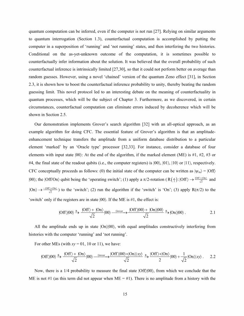
quantum computation can be inferred, even if the computer is not run [27]. Relying on similar arguments

to quantum interrogation (Section 1.3), counterfactual computation is accomplished by putting the

computer in a superposition of ‘running’ and ‘not running’ states, and then interfering the two histories.

Conditional on the as-yet-unknown outcome of the computation, it is sometimes possible to

counterfactually infer information about the solution. It was believed that the overall probability of such

counterfactual inference is intrinsically limited [27,30], so that it could not perform better on average than

random guesses. However, using a novel ‘chained’ version of the quantum Zeno effect [31], in Section

2.3, it is shown how to boost the counterfactual inference probability to unity, thereby beating the random

guessing limit. This novel protocol led to an interesting debate on the meaning of counterfactuality in

quantum processes, which will be the subject of Chapter 3. Furthermore, as we discovered, in certain

circumstances, counterfactual computation can eliminate errors induced by decoherence which will be

shown in Section 2.5.

Our demonstration implements Grover’s search algorithm [32] with an all-optical approach, as an

example algorithm for doing CFC. The essential feature of Grover’s algorithm is that an amplitude-

enhancement technique transfers the amplitude from a uniform database distribution to a particular

element ‘marked’ by an ‘Oracle type’ processor [32,33]. For instance, consider a database of four

elements with input state |00⟩: At the end of the algorithm, if the marked element (ME) is #1, #2, #3 or

#4, the final state of the readout qubits (i.e., the computer registers) is |00⟩, |01⟩, |10⟩ or |11⟩, respectively.

CFC conceptually proceeds as follows: (0) the initial state of the computer can be written as |ψin⟩ = |Off⟩

|00⟩; the |Off/On⟩ qubit being the ‘operating switch’; (1) apply a π/2-rotation ( ( ) |Off |On2 2

R : |Offπ ⟩+ ⟩⟩ → and

|Off |On2

|On − ⟩+ ⟩⟩ → ) to the ‘switch’; (2) run the algorithm if the ‘switch’ is ‘On’; (3) apply R(π/2) to the

‘switch’ only if the registers are in state |00⟩. If the ME is #1, the effect is:

GroverR R |Off |On |Off |00 |On |00|Off |00 |00 |On |002 2

⟩ + ⟩ ⟩ ⟩ + ⟩ ⟩⟩ ⟩ → ⟩ ⎯⎯⎯→ → ⟩ ⟩ . 2.1

All the amplitude ends up in state |On⟩|00⟩, with equal amplitudes constructively interfering from

histories with the computer ‘running’ and ‘not running’.

For other MEs (with xy = 01, 10 or 11), we have:

GroverR R |Off |On|Off | |Off |00 |On | |Off |On 1|00 |On |22 2

00 |002

xy xy⟩ ⟩+ ⟩ ⟩ ⟩+ ⟩⟩

⟩ + ⟩⟩ ⟩ → ⟩ ⎯⎯ → ⟩⎯→ + ⟩ . 2.2

Now, there is a 1/4 probability to measure the final state |Off⟩|00⟩, from which we conclude that the

ME is not #1 (as this term did not appear when ME = #1). There is no amplitude from a history with the

16

computer ‘running’ in this outcome; therefore, we can conclude that the ME is not #1 without the

computer ‘running’. Below, we will specify precisely what is meant by ‘running’, in the context of two

possible physical implementations. Methods to counterfactually determine the actual outcome will be

discussed in Section 2.3.

2.2 The experiment

An optical realization of CFC is shown in Figure 2.1 as an interferometer. We used the optical circuit in

reference [34] for Grover’s algorithm (shown as a black box in Figure 2.1, and discussed in detail in

Section 2.2.1), with slight changes to improve performance. This optical circuit takes in a single photon in

path ‘a’ with H (horizontal) polarization, that is, |aH⟩. The output path ‘a’ or ‘b’ and polarization H or V

(vertical) of the photon depend on the ME: #1 → |aH⟩, #2 → |aV⟩, #3 → |bH⟩ and #4 → |bV⟩. Such

single-photon encoding, though not scalable, suffices for our pedagogical purpose. Figure 2.2.a shows

that the algorithm as realized operates quite precisely, with an average error of less than 2.6%. This is, to

our knowledge, the most precise implementation of a quantum algorithm to date in any physical system.

To realize CFC, the path lengths of the interferometer in Figure 2.1 are adjusted to give destructive

interference at detector D1 when the ME is #1; that is, if the photon traverses both paths indistinguishably,

it is definitely detected at D5 (Figure 2.1). If the ME is not #1, there is no amplitude exiting the search

algorithm in the |aH⟩ mode, and no amplitude from the algorithm can reach the second beam-splitter (BS),

thus eliminating the destructive interference at D1. Therefore, this time there is a 1/4 probability of

detecting the photon at D1, indicating that the ME is not #1, even though the photon came from the

Figure 2.1: Realization of CFC is as an optical interferometer. By means of a 50/50 beam splitter (BS)(which serves as a π/2-rotation), an H-polarized single photon is put in a superposition of passing and notpassing through the algorithm, encoding the ‘operating switch’ in different spatial modes, ‘On’ and ‘Off’.Then on a second 50/50 BS, the two histories are interfered only if the photon after the algorithm is in themode |aH⟩. The modes |aH⟩ and |aV⟩ are distinguished via a polarizing beam splitter (PBS) whichtransmits H-polarized and reflects V-polarized light.

17

algorithm-free path (that is, the computer did not run). Other possibilities are that with probability 1/2 we

find out the answer but the photon comes from the algorithm (D2, D3 or D4), and with probability 1/4 we

detect the photon at D5 (after it has traveled the algorithm-free path) leading to no definite information (as

a detection also occurs at D5 if ME is #1). The efficiency of CFC can be quantified as

( )1 1D D Grover/ 1/ 3P P Pη = + = ; where 1DP is the probability of measuring the photon at D1, a CFC; and

GroverP is the probability of the photon passing through the algorithm. The value η = 1/3 assumes 50/50

BSs; as we discuss below, by using an unbalanced interferometer, one can in principle increase this to 1/2.

In Section 2.3 we discuss mechanisms to achieve η → 1. Also, see Section A.1 for a side discussion on a

modified version of CFC that interrogates all database elements simultaneously to determine the ME

itself; however, this modified version is also limited to η = 1/2.

Experimentally, we used an equivalent but more stable interferometer configuration, discussed in

Section 2.2.2; our CFC system performed as indicated in Figure 2.2.b, with an efficiency

0.319 0.009η⟨ ⟩ = ± (averaged over ME ≠ #1). The interrogation interferometer had an intrinsic visibility

Figure 2.2: Experimentally determined probabilities for the output state of 670-nm single photonsconditionally prepared through downconversion [38]. a, The performance of the search algorithm. Thetotal probability of finding the photon in any incorrect output port is 2.6% (averaged over MEs); thus, theME could be accurately determined with a single photon passing through the algorithm. b, Output stateprobabilities for the setup in Fig. 1. Grid lines closest to data points represent theory. We attribute slightdeviations from theory to imperfect beam splitting ratios, imperfect mode matching (apparently fromwave-front distortions in various elements), and imperfect path-length balancing.

18

of 97%, implying imperfect destructive interference at the D1 output when the ME was #1. A detection at

the D1 output can thus no longer indicate a CFC with 100% certainty. We characterize this feature in

terms of SuccP ; the probability of a successful CFC upon a detection at the interrogation detector D1 is then

given by: ( )1 1 1Succ|# D |# D |#1 D |#/i i iP P P P= + . Here the probabilities are conditional on the ME (i= 2, 3, 4). In the

experiment we achieved SuccP⟨ ⟩ = 0.943± 0.009.

If one replaces the first (second) 50/50 beam splitter by a highly reflecting (transmitting) one, reducing

the amplitude passing through the algorithm, η can be increased [35] to a maximum value of 1/2. We

tested this (using attenuated coherent states11) with a 5/95 BS, achieving η⟨ ⟩ = 0.472 ± 0.007 (0.487

theoretically), with a slight decrease in the CFC success: Succ 87.7 0.009P = ± . We now give a detailed

discussion of the experiment.

2.2.1 Experimental encoding of the search algorithm

Suppose we wish to locate a particular entry in a large unsorted database of N elements. Classically this is

accomplished by comparing the elements one by one with the target, on average taking N/2 queries.

Grover’s algorithm makes use of the parallelism supported by the superposition of quantum states to

locate the element in only N∼ queries [33]. In general, n qubits are used to encode a database of

2nN = elements; however, for simplicity we will limit our initial discussion to four elements. The initial

state of the qubits is prepared to be in an equal-amplitude superposition of each of the database elements,

i.e., ( )12 | | |1 |00⟩+ 01⟩+ 0⟩+11⟩ for two qubits, encoding four database elements. The algorithm uses an

‘Oracle’ that simultaneously evaluates a certain function for all elements (by means of comparing the

elements and the target) and marks the element being searched for with a minus sign (π phase shift). For

example, ( )12 | | |1 |00⟩+ 01⟩− 0⟩+11⟩ will be the state of the two qubits after the ‘Oracle’ if the ME is #3.

Amplitude enhancement of the ME is then accomplished by applying an ‘inversion about the mean’

operation (a phase shift in a conjugate basis), consisting of three steps: (1) Apply a Walsh-Hadamard

(WH) transform to each qubit; (2) apply a π-phase shift to all but database element #1 (|00⟩); (3) apply a

WH transform to each qubit. This operation transfers amplitude from the unmarked elements to the

11 We used an attenuated laser beam (coherent states) to perform this part of the experiment as opposed to using

true single-photon states from the downconversion source. The attenuation level was such that there is much less than one photon on average inside of the interrogation interferometer. Single photons and coherent states are expected to behave identically as far as linear optics is concerned. The interpretation of a counterfactual outcome does not change, except that now, although very small, there is a chance that a second photon is in the interferometer, and that second photon may have passed through the computer (the search algorithm here) while the first one is signaling a counterfactual result. In our implementation, this probability was less than 0.1%.

19

marked one. For a database of four elements, a single iteration (one query) yields the answer with unit

probability. (For N > 4 elements, one will need to run the oracle and inversion operations 4Nπ∼ times

[33]. Also, for N > 4 the algorithm in general outputs non-orthogonal states as answers; therefore, the

answer cannot be obtained with unit probability.) As an example of the entire algorithm, if the ME is #3

the state will evolve as:

( ) ( )

( )( ) ( )( ) ( )( ) ( )( )

[ ]

WH Oracle

(1)

(2)

(3)

|00 |00 |01 |10 |11 |00 |01 |10 |11

|0

1 12 21 2

1 ( ) ( )2

|1 |0 |1 |0 |1 |0 |1 |0 |1 |0 |1 |0 |1 |0 |1

|00 |01 |10 |11

|10

⟩ ⟩+ ⟩+ ⟩+ ⟩ ⟩+ ⟩− ⟩+ ⟩

⟩+ ⟩ ⟩+ ⟩ + ⟩+ ⟩ ⟩− ⟩ − ⟩− ⟩ ⟩+ ⟩ + ⟩− ⟩ ⟩− ⟩

⟩− ⟩+ ⟩

→ ⎯⎯⎯→

⎡ ⎤→ ⎣ ⎦

→ − −

→

+ ⟩

⟩.

2.3

Likewise if the ME was #1, #2, or #4, the final state of the qubits would be |00⟩, |01⟩, and |11⟩,

respectively.

Experimentally, our first qubit is encoded in two orthogonal polarization states, horizontal ( |H⟩) and

vertical (|V⟩) of a single photon, corresponding to |0⟩ and |1⟩ logical states of the qubit; our second qubit is

encoded in two non-overlapping spatial modes, labeled |a⟩ and |b⟩. These two qubits act as both the input

and output registers of our quantum computer. Using this single-photon two-qubit encoding, two-qubit

gates, which otherwise require effective photon-photon interactions, become trivial with only linear

optical elements [36]. Single-photon multi-qubit approaches to quantum computing are not scalable

Figure 2.3: The schematic of the optical circuit realizing the search algorithm in a database of fourelements. The circuit is implemented as a double Sagnac interferometer. See the text for descriptions.

20

(requiring an exponential increase in resources [37]), but the algorithm as realized is fully quantum and

sufficient for our pedagogical purpose. Experimentally, a half-wave plate (HWP) oriented at 22.5° acts on

the polarization qubit as a WH gate up to a phase factor, and a 50/50 beam-splitter (BS) realizes the same

gate for the spatial qubit [36]. In order to realize the conditional phase shift of step (2) of Equation 2.3, a

birefringent material can be inserted into spatial path ‘a’, which will induce a relative π-phase shift for H

polarization. (A non-birefringent element in path ‘b’ will compensate for any induced phase on |aV⟩.) An

optical circuit for Grover’s algorithm can thus be constructed [34], with the ‘Oracle’ simulated by

controllable birefringence in paths ‘a’ and ‘b’. Here we use a compiled version of the circuit,

implemented as a double Sagnac interferometer (Figure 2.3). This interferometer design is self-stabilized

against drift, since any path length variation equally affects both clockwise (CW) and counter-clockwise

(CCW) propagation directions. To implement the ‘Oracle’ we use four pixels of custom-made liquid

crystal (LC) phase retarders, enabling us to induce relative π-phase shifts independently on each

element12. Phase retardence data for the particular LCs can be found in Section A.2.

2.2.2 Details of the experiment

As described, we apply the idea of counterfactual computation (CFC) to Grover’s search algorithm by

placing it in one arm of an interferometer. In particular, we show a Mach-Zehnder interferometer in

Figure 2.1. However, as mentioned, we followed a different (but equivalent) approach due to

interferometric stability issues. The experiment is performed using a two-layered optical design: The

incoming beam is first sent through a calcite beam displacer, vertically separating the H and V orthogonal

linear polarization components by 4 millimeters (see Figure 2.4). After passing through a linear polarizer

(LP) at 45° (which automatically prepares the correct polarization superposition state output of the first

WH gate of Equation 2.3), the beams in the two layers have the same polarization. The two layers

traverse the same optical elements except for the ‘Oracle’, i.e, the upper layer ‘On’ goes through the

algorithm and the lower layer ‘Off’ does not. The optical path lengths of the ‘Off’ layer are adjusted so

that all the amplitude in this layer leaves the double Sagnac interferometer in path ‘a’ with H polarization.

The ‘a’ paths in the ‘On’ (upper) and ‘Off’ (lower) layers are then twisted using a Dove prism, so that

they are horizontally side by side where they are recombined on a BS. If the output of the algorithm is

‘aH’, destructive interference at this final BS then leads to no counts at detector D1, as required for CFC.

12 The LCs are driven by a homemade circuit with four channels of 2 kHz square waves with independently

variable amplitudes. Note that square waves with given amplitude (typically in the range 0-10V peak-to-peak) induce a constant phase retardence on the polarization component along the optic axis of the LC.

21

The circuit is fed by 670-nm single photons produced by non-degenerate optical spontaneous

parametric downconversion in a 0.6-mm thick BBO crystal (cut at θ = 33.9° for type-I phase-matching),

pumped by the 351-nm line of an Argon-ion laser. Conditional on the detection of a trigger photon at 737

nm (at Detector T of Figure 2.4), a localized 670-nm single photon is prepared13 [38]. The wavelength is

selected by a 2-nm bandpass interference filter, corresponding to a coherence length of ~λ2/∆λ = 224 µm;

the interferometer path lengths therefore had to be balanced much better than this to display high

visibility. The interferometer output ports were analyzed using rotatable LPs (instead of PBSs); the

photons were collected using multimode fibers, and detected with single-photon counting modules (Si

avalanche photodiodes).

The optical sub-circuit realizing only Grover’s search is characterized by blocking the algorithm free

(lower) path of the interrogation interferometer. Data shown in Figure 2.2.a indicate that a single photon

can determine the ME with ~97.5% accuracy. The CFC interrogation system is activated by unblocking

the algorithm-free path; as predicted, when the marked element was not #1, we registered photons at

detector D1 of Figure 2.4 (equivalently detector D1 of Figure 2.1) ~1/4 of the time, indicating a

counterfactual computation. (See the results in Figure 2.2.b.)

13 The 670-nm signal photons are coupled into a single-mode fiber and then launched into the interferometers for

assuring high mode quality. The trigger photons are collected on the conjugate side of the downconversion cones into a free-space detector after an iris. The 351-nm pump laser power was ~150 mW, the coincide rate was ~104/s, and the singles-to-coincidences ratio on the signal side was ~5-10%.

Figure 2.4: The optical circuit used for the CFC experiment. Detector numbers correspond to those in thesimpler schematic shown in Figure 2.1. The Dove prism rotates the two beams (‘On’ and ‘Off’ paths)from the vertical plane to the horizontal plane. See the text for other descriptions.

22

2.3 High efficiency methods

As discussed above, the efficiency of our simple approach is, theoretically 1/3, but can be increased to 1/2

by using non-50/50 BSs, i.e., by reducing the amplitude in the ‘On’ state. Remarkably, the efficiency of

counterfactual computation can actually be increased to unity by using the quantum Zeno effect [27]:14

The switch is rotated successively in small steps ( ( )R 2 :|Off cos |Off sin |Onθ θ θ⟩ → ⟩ + ⟩ and

|On sin |Off cos |Onθ θ⟩ → − ⟩ + ⟩ ; 2 , integers 1N Nπθ = ∈ ,) from state |Off⟩ to |On⟩; and the output

registers are monitored at each step. If the ME is #1, measurements on the output registers result in |00⟩

without affecting the evolution due to rotations, leaving the system in |On⟩|00⟩ after N rotations. However,

if the ME is not #1, then the system evolves as:

( )R Grover Measure|Off |00 cos |Off sin |On |00 cos |Off |00 sin |On | cos |00xyθ θ θ θ θ⟩ ⟩ → ⟩ + ⟩ ⟩ → ⟩ ⟩ + ⟩ ⟩ → ≈ ⟩ . 2.4

The measurement on the output registers results in state |00⟩; leaving the computer in the |Off⟩ state

with probability ( )22cos Nπ . After a total of N cycles, the probability of finding the system in state

|Off⟩|00⟩ is ( )22cos N

Nπ which tends to 1 as N→∞. Thus, if the ME is not #1, the final state is |Off⟩|00⟩

without the computer running; and if the ME is #1, the final state is |On⟩|00⟩; that is, this time the

computer runs. Note that at best one can exclude a single value of the ME with these techniques.

The novel ‘chained Zeno effect’ that we developed will permit us to counterfactually determine the

actual ME with η →1. The strategy is to place the above ‘Zeno scheme’ inside another one, to avoid the

computer running even if the ME is #1. For this purpose we use a third ‘switch’ state |Off ′⟩, in addition to

|Off⟩ and |On⟩; and define an additional rotation R′ to couple |Off ′⟩ to |Off⟩:

( )R ' 2 ' : |Off ' cos '|Off ' sin '|Offθ θ θ⟩ → ⟩ + ⟩ and |Off sin '|Off ' cos '|Offθ θ⟩ → − ⟩ + ⟩ ; 2 '' Nπθ = . A possible

optical implementation of the technique is shown in Figure 2.5.a. A single photon starts in cavity ‘Off ′’.

Using active optical elements (Pockels cells), a small amount of amplitude is exchanged between ‘Off ′’

and Off via BS1. The small amplitude then performs the high-efficiency quantum Zeno cycles described

above (N times between cavities ‘Off’ and ‘On’)15. If the ME ≠ #1, the small amplitude component

14 Note that the approach here should not be confused with the interesting proposal to combine two-photon

absorption and the quantum Zeno effect to enable efficient optical quantum computation [46], nor with the suggestion to use quantum interrogation inside Grover’s search algorithm [130].

15 Using a PBS and a PC, a single photon can be switched into cavity ‘Off ′’ initially (Figure 2.5.a). Next, by firing the Pockels cells at appropriate times, cavities ‘Off ′’ and ‘Off’ are allowed a single coherent amplitude exchange via BS1, after which the cavities are isolated again. While the vast majority of the amplitude is cycling in

23

effectively stays in cavity ‘Off’. But if ME = #1, then first, all the small amplitude component transfers to

cavity ‘On’, and then, via the Pockels cell in cavity ‘On’, is actively absorbed at A1.16 Now the entire

procedure starting with the amplitude exchange between ‘Off ′’ and ‘Off’ is repeated, a total of N ′ times.

cavity ‘Off ′’, the small amount of amplitude that has been allowed to leak into cavity ‘Off’ performs the high-efficiency quantum Zeno cycles described in the text (N times between cavities ‘Off’ and ‘On’).

16 At each step, the amplitude exiting the algorithm is directed to an absorber (A2 or A3 in Figure 2.5.a) if the ME is different from #1, effectively projecting the leaked amplitude into cavity ‘Off’, assuming 1N . In contrast, if the ME is #1, at the end of N cycles all of the small amplitude component has coherently moved into cavity ‘On’; when the Pockels cell in this cavity is fired to terminate the amplitude at A1, no amplitude is left in either cavity ‘Off’ or ‘On’. In fact, this effectively projects the state into cavity ‘Off ′’, assuming ' 1N .

Figure 2.5: Proposed set-up for the ‘chained Zeno effect’. Three cavities correspond to three states of theswitch (|Off ′⟩, |Off⟩ and |On⟩), separated by BSs—the rotation operators. Pockels cells (PCs) rotate thepolarization by 90° on demand; half-wave plates (HWP) at 45° rotate the polarization by 90°. GSA,Grover’s search algorithm. a, Interrogation for element #1. A1-A3 are absorbers. b, Settings for theinterrogation of different elements. c, Settings for the qubit-by-qubit interrogation technique. GSA† un-does the action of GSA d, Configuration for the error suppression technique described in Section 2.5.π-PS induces a π-phase shift on path ‘b’; HWP at 0° induces a π-phase shift on V polarization. e,Probability of successful interrogation for the set-up in a, as a function of the cycling parameters N ′ andN (numerically evaluated).

24

At the end of N × N ′ total cycles, upon successful operation (i.e., no absorption event), if ME = #1 (≠ #1)

then the photon will be measured in cavity ‘Off ′’ (‘Off’) with probability approaching one (Figure 2.5.e)

as N ′→∞ ( N/N ′→∞). In neither of these cases does the computer ‘run’. One can then re-interrogate for

the other elements one by one—thereby identifying the ME counterfactually—by changing the

connections to the algorithm (Figure 2.5.b). Curves in Figure 2.5.e characterize a lossless system; for

large N ′, N, even small losses become detrimental [12], limiting the achievable performance in any real

system.

The necessity to interrogate database elements one by one would negate the quantum speed-up

advantage. However, it is possible to circumvent this by interrogating the logical value of each qubit one

by one instead. To do this, we need to implement both the search algorithm and its adjoint—which

undoes the search—and we need to perform the measurements (giving rise to the Zeno effect) between

the algorithm and its adjoint. The first (second) optical circuit in Figure 2.5.c can be used in cavity ‘On’,

to interrogate for the logical value of the first (second) qubit. If the value of the first (second) qubit is ‘a’

(H), then, at the end of the cycles, the photon will be measured in cavity ‘Off ′’; likewise if the value is

‘b’ (V), then the photon will be measured in cavity ‘Off’. In neither case does the computer (nor its

adjoint) run. (See Section 2.3.1 for more details, including the quantum circuit diagram of this method.)

2.3.1 Details of the qubit­by­qubit interrogation technique

The ‘qubit-by-qubit’ interrogation technique was introduced in Section 2.3, by which the output qubits

from a search algorithm can be determined one by one, without the algorithm actually running. This

represents an exponential speed-up over the basic scheme, which only interrogates for the database

elements one by one. Here we present a detailed explanation of the technique. Figure 2.6 shows the

corresponding quantum circuit diagram. (General information on quantum circuit diagrams can be found

in reference 33.) The diagram flows from left to right. A single line represents a qubit, and a double line

represents a classical bit. The initial state and the name of each qubit is indicated at the beginning (left

side) of the diagram.

The qubits ‘CF1’ and ‘CF2’ are the counterfactual output qubits, which at the end indicate the search

result |xy⟩ (xy = 00, 01, 10, or 11) that would have been output by the search algorithm GSA if it were to

run, without the search algorithm actually ‘running’. (Note that, the algorithm has to be ready to run, i.e.,

the associated laser pulses, Pockels cell or liquid crystal voltages, etc., must still be applied.) The qubit

‘S1’ is an ancillary ‘subroutine’ qubit, and the qubits ‘1’ and ‘2’ are both the input and output registers of

the search algorithm.

25

At the beginning, all the qubits are initialized to |0⟩. The first ‘routine’, which counterfactually

determines the first qubit of the search result, starts with a 2θ ′-rotation ( 2 '' Nπθ = ) on the qubit ‘CF1’

(after which the state has evolved to 'CF1'| cos '|0 sin '|1θ θΨ ⟩ = ⟩ + ⟩ ), and continues with the implementation

of a ‘subroutine’ only if the state of ‘CF1’ is |1⟩. This ‘subroutine’ starts with a 2θ-rotation ( 2Nπθ = ) on

the qubit ‘S1’ (at this stage 'CF1','S1'| cos '|00 sin 'cos |10 sin 'sin |11θ θ θ θ θΨ ⟩ = ⟩ + ⟩ + ⟩ ), and continues by

implementing the search algorithm GSA only if ‘S1’ is in state |1⟩ (at this stage

'CF1','S1','1','2'| cos '|00 |00 sin 'cos |10 |00 sin 'sin |11 |xyθ θ θ θ θΨ ⟩ = ⟩ ⟩ + ⟩ ⟩ + ⟩ ⟩ ). Notice that the |00⟩, |10⟩ and |11⟩

Figure 2.6: The quantum circuit diagram of the high-efficiency qubit-by-qubit-interrogation technique. Ryimplements a single-qubit rotation about the y-axis. The square boxes with ‘meters’ represent single-qubitmeasurements in the computational (|0⟩, |1⟩) basis; they output the result (0 or 1) to the classical bitchannel and the corresponding state to the qubit channel. GSA implements the search algorithm andGSA† implements the adjoint of it, i.e., ‘un-does’ the search. Controlled-gate operations work as follows:The gate is implemented only if the control qubit, i.e., the qubit which the gate is connected to with a lineand a filled circle, is in state |1⟩. Vertical dashed lines intersecting the qubit lines represent cycles: Thestate of a qubit at the right dashed line is fed back to the same qubit channel at the previous dashed line,and allowed to evolve again. Cycles are carried out the number of times specified on top of the braceconnecting the dashed lines. Note that the cycles are conditioned on the classical bit being in state ‘0’(indicated by a hollow circle), i.e., if the classical bit is ‘1’, then GSA has run, and the whole circuit halts.

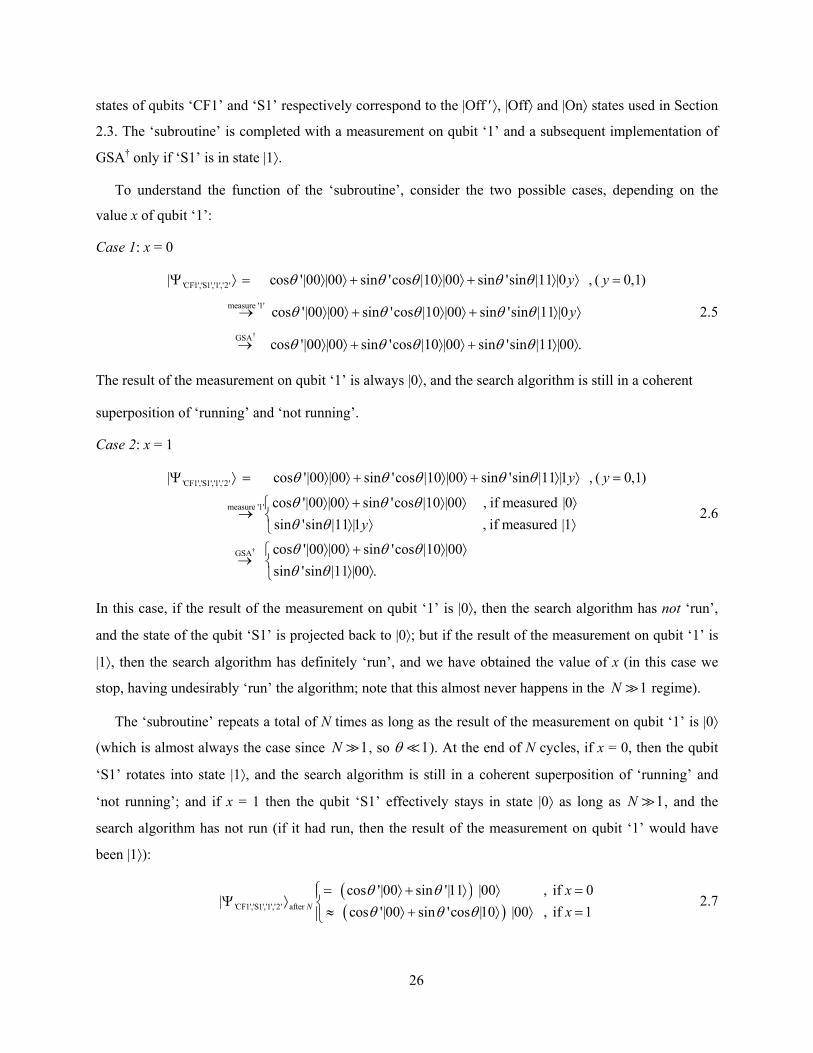
26

states of qubits ‘CF1’ and ‘S1’ respectively correspond to the |Off ′⟩, |Off⟩ and |On⟩ states used in Section

2.3. The ‘subroutine’ is completed with a measurement on qubit ‘1’ and a subsequent implementation of

GSA† only if ‘S1’ is in state |1⟩.

To understand the function of the ‘subroutine’, consider the two possible cases, depending on the

value x of qubit ‘1’:

Case 1: x = 0

†

'CF1','S1','1','2'

measure '1'

GSA

| cos '|00 |00 sin 'cos |10 |00 sin 'sin |11 |0 0,1

cos '|00 |00 sin 'cos |10 |00 sin 'sin |11 |0

cos '|0

y y

y

θ θ θ θ θ

θ θ θ θ θ

θ

Ψ ⟩ = ⟩ ⟩ + ⟩ ⟩ + ⟩ ⟩ , ( = )

→ ⟩ ⟩ + ⟩ ⟩ + ⟩ ⟩

→ 0 |00 sin 'cos |10 |00 sin 'sin |11 |00θ θ θ θ⟩ ⟩ + ⟩ ⟩ + ⟩ ⟩.

2.5

The result of the measurement on qubit ‘1’ is always |0⟩, and the search algorithm is still in a coherent

superposition of ‘running’ and ‘not running’.

Case 2: x = 1

'CF1','S1','1','2'

measure '1'

| cos '|00 |00 sin 'cos |10 |00 sin 'sin |11 |1 0,1

cos '|00 |00 sin 'cos |10 |00 if measured |0

sin 'sin |11 |1

y y

y

θ θ θ θ θ

θ θ θθ θ

Ψ ⟩ = ⟩ ⟩ + ⟩ ⟩ + ⟩ ⟩ , ( = )

⟩ ⟩ + ⟩ ⟩ , ⟩ →

⟩ ⟩

†GSA

if measured |1

cos '|00 |00 sin 'cos |10 |00

sin 'sin |11 |00θ θ θθ θ

⎧⎨ , ⟩⎩

⟩ ⟩ + ⟩ ⟩⎧→ ⎨ ⟩ ⟩.⎩

2.6

In this case, if the result of the measurement on qubit ‘1’ is |0⟩, then the search algorithm has not ‘run’,

and the state of the qubit ‘S1’ is projected back to |0⟩; but if the result of the measurement on qubit ‘1’ is

|1⟩, then the search algorithm has definitely ‘run’, and we have obtained the value of x (in this case we

stop, having undesirably ‘run’ the algorithm; note that this almost never happens in the 1N regime).

The ‘subroutine’ repeats a total of N times as long as the result of the measurement on qubit ‘1’ is |0⟩

(which is almost always the case since 1N , so 1θ ). At the end of N cycles, if x = 0, then the qubit

‘S1’ rotates into state |1⟩, and the search algorithm is still in a coherent superposition of ‘running’ and

‘not running’; and if x = 1 then the qubit ‘S1’ effectively stays in state |0⟩ as long as 1N , and the

search algorithm has not run (if it had run, then the result of the measurement on qubit ‘1’ would have

been |1⟩):

( )( )'CF1','S1','1','2' after

cos '|00 sin '|11 |00 , if 0|

cos '|00 sin 'cos |10 |00 , if 1N

xx

θ θθ θ θ

⎧= ⟩ + ⟩ ⟩ =⎪Ψ ⟩ ⎨ ≈ ⟩ + ⟩ ⟩ =⎪⎩ 2.7

27

Now we return to the ‘routine’, which is completed with a measurement on qubit ‘S1’. To understand

the function of the ‘routine’, consider the two possible cases, depending on the value x of qubit ‘1’:

Case 1: x = 0

( )'CF1','S1','1','2'

measure 'S1'

| cos '|00 sin '|11 |00

cos '|00 |00 if measured |0

sin '|11 |00 if measured |1

θ θ

θθ

Ψ ⟩ = ⟩ + ⟩ ⟩

⟩ ⟩ , ⟩⎧→ ⎨ ⟩ ⟩ , ⟩⎩

2.8

If the result of the measurement on qubit ‘S1’ is |0⟩, then the ‘subroutine’ has not ‘run’ (neither has the

search algorithm), and the state of the qubit ‘CF1’ is projected back to |0⟩; but if the result of the

measurement on qubit ‘S1’ is |1⟩, then the ‘subroutine’ has definitely run (and so has the search

algorithm), and we have obtained the value of x (note that this almost never happens in the ' 1N

regime).

Case 2: x = 1

( )

( )'CF1','S1','1','2'

measure 'S1'

| cos '|00 sin 'cos |10 |00

cos '|00 sin 'cos |10 |00

θ θ θ

θ θ θ

Ψ ⟩ ≈ ⟩ + ⟩ ⟩

→ ⟩ + ⟩ ⟩ 2.9

In this case, the result of the measurement on qubit ‘S1’ is always |0⟩, and the ‘subroutine’ is still in a

coherent superposition of ‘running’ and ‘not running’; but notice that, when x = 1, the search algorithm

does not run (as explained in the ‘subroutine’ paragraphs above).

The ‘routine’ repeats a total of N ′ times as long as the result of the measurement on qubit ‘S1’ is |0⟩

(which is almost always the case since ' 1N ). At the end of N ′ cycles, if the first qubit of the search

result is |0⟩ (|1⟩), then the counterfactual output qubit ‘CF1’ effectively stays in state |0⟩ (effectively

rotates into state |1⟩) as long as ' 1N ( / ' 1N N ), and the algorithm never ‘runs’:

'CF1','S1','1','2' final

|0 |000 , if 0|

|1 |000 , if 1xx

≈ ⟩ ⟩ =⎧Ψ ⟩ ⎨≈ ⟩ ⟩ =⎩

2.10

The CFC success probability of this whole ‘routine’, i.e., the probability that the measurements on

qubit ‘1’ and ‘S1’ never result in |1⟩, is the same as that given in Figure 2.5.e as a function of N and N ′.

The next ‘routine’, which counterfactually determines the second qubit of the search result, i.e., the

value of y, is accomplished in a very similar way, and the result is output to the qubit ‘CF2’. Similarly we

could continue to perform a counterfactual search on an n-qubit database, by appending more ‘routines’.

28

2.3.2 Discussion of cases involving more general algorithms

So far the discussion of CFC was centered on using GSA in a database of four elements. However, the

discussion would be valid for any quantum algorithm. As relevant examples, Section 2.3.2.a considers

CFC when searching a larger database, where non-orthogonal output states from the algorithm are

allowed, and Section 2.3.2.b considers the case where the ‘Oracle’ of the search algorithm ends up in a

quantum superposition of marking different elements.

2.3.2.a CFC when searching a larger database

So far we limited our discussion on CFC to Grover’s search algorithm (GSA) in a database of four

elements. The methods that we presented can also be used for searching a larger database (or even for

different quantum computation algorithms). However, for a database with more than four elements (or if

there is more than one ME), GSA by its nature outputs non-orthogonal states as answers. That is, the

algorithm outputs |Ψ1⟩ if ME = #1, |Ψ2⟩ if ME = #2, and so on; however these states may have some

overlap with each other, i.e., ⟨Ψi|Ψj⟩ ≠ 0.

Therefore, as a generic scenario, the states output from a quantum computer for different answers need

not necessarily be completely orthogonal to each other. We would like understand whether the CFC

methods developed up to this point will still function properly with this new assumption. As we will see,

with slight modifications, in principle the answer is: yes the methods will still work. Our discussion will

take a generic GSA as an example.

We will begin with the simple CFC scheme (the analog of Figure 2.1). As an example, in order to

counterfactually determine that the ME is not #1, a unitary operator can be applied to the output of GSA

which would rotate |Ψ1⟩ (the particular state the algorithm outputs when ME = #1) into |00...0⟩, and

consequently |Ψ2⟩, |Ψ3⟩,... into different but not necessarily orthogonal states. Then, ME = #1 would be

the only case in which a complete destructive interference at detector D1 (analog of Figure 2.1) will be

achieved. If ME is not #1 photons can be detected at D1. Thus all necessary conditions for CFC would be

satisfied.

For the case of ‘element-by-element’ ‘chained’ Zeno CFC, similarly, when we use the unitary operator

to rotate |Ψ1⟩ into |00...0⟩ at the output of GSA (the analog of Figure 2.5.a&b), ME = #1 would be the

only case which would allow the amplitude in ‘Off’ to coherently move to ‘On’; the other MEs would

result in (partial) absorption, giving rise to the Zeno effect to keep the amplitude in ‘Off’. Note that

although the absorption is only partial in this case, the Zeno effect will be enhanced as N –the number of

‘Off’-‘On’ inner cycles– increases. Therefore, all the necessary conditions for CFC can again be satisfied.

29

In the case of ‘qubit-by-qubit’ ‘chained’ Zeno CFC (the analog of Figure 2.5.a&c), one might think

that for the adjoint of the algorithm (GSA†) to function properly, the outputs from GSA before the

measurement step need to be orthogonal to each other for different MEs. However, we have found that, in

principle, by replacing the standard measurement step between GSA and GSA† with a POVM (Positive

operator-valued measure) type measuring arrangement, the CFC scheme can be made to work. POVMs

are generalized quantum measurements employing ancillary degrees of freedom [33,39], and a brief

discussion can be found in Section A.3.17 For the purpose of the current discussion, a circuit UPOVM that

would be implementing the unitary part (including the ancillary degree of freedom) of the desired POVM

and its adjoint U†POVM would be placed between GSA and GSA†.18 The purpose of UPOVM is to sort the

ME-dependent non-orthogonal output states into orthogonal states and an additional ‘error’ state19. The

actual measurement step (i.e., the blocking of one qubit value (analog of Figure 2.5.c)) should take place

between UPOVM and U†POVM (with the error port never blocked). Under these circumstances, the arguments

reduce to the case of the ‘element-by-element’ CFC described in the preceding paragraph, and thus, the

‘qubit-by-qubit’ CFC can be made to work again.

2.3.2.b If the ‘Oracle’ of the search algorithm were to be in a quantum superposition

Here we briefly discuss what happens if the ‘Oracle’ of the search algorithm ends up in a quantum

superposition of marking different elements to begin with (this could happen, for example, if we were

searching a ‘quantum database’, and the ‘target’ was not a single element but a quantum superposition of

elements). In this case, the output of the algorithm could become entangled with the ‘Oracle’ itself, and

consequently, so could the output of CFC. To be concrete, assume that the ‘Oracle’, whose ‘inner-

working’ we represent simply as |ΨOracle⟩, is in a superposition of marking element #1 and #2:

( )12

| |#1⟩+ #2⟩ . Then, the simplest version of CFC (the analog of Equations 2.1&2.2) would evolve as:

( ) ( )

( ) ( )

R

Grover

1 12 2

R

1 12 2

| | 1|Off |00 | |Off |On |00 | |Off |On |002 2

1 | |Off |On |00

| |Off |00 |On |012

1 1| | On |002

#1⟩+ #2⟩ ⎡ ⎤⟩ ⟩ #1⟩ ⟩+ ⟩ ⟩+ #2⟩ ⟩+ ⟩ ⟩⎣ ⎦

⎡ ⎤#1⟩ ⟩+ ⟩ ⟩+ #2⟩ ⟩ ⟩+ ⟩ ⟩⎣ ⎦

#1⟩ ⟩

→

→ ⟩ +

→

( )1 12 2

| |Off |On |00 |On |01 .2

⎡ ⎤#2⟩ ⟩+ ⟩ ⟩ + ⟩ ⟩⎣ ⎦

2.11

17 Note also that a quantitative example of a POVM is also used in Section A.1. 18 A linear optical circuit can in principle be devised to implement UPOVM, but we have not investigated this. 19 The former alone, without the additional ‘error’ state, is not possible with a unitary transformation (i.e., a norm

changing transformation would be required). We see that a POVM distinguishes non-orthogonal states, but this comes at the cost of not distinguishing at all (i.e., when the ‘error’ state is obtained).

30

As we see, we obtain a coherent superposition of the two different cases that we investigated in

Equations 2.1&2.2, but upon a measurement on the system, all the arguments that we made both

qualitatively and quantitatively still apply. That is, the measurement projects out one of the cases.

However, note that the state of the ‘Oracle’ must not explicitly become entangled with the ‘switch’ during

CFC (i.e., the state of the ‘Oracle’ must remain the same for both ‘On’ and ‘Off’ histories between two

rotations (R) on the ‘switch’ qubit in Equation 2.11); otherwise such entanglement would make the ‘On’

and ‘Off’ histories distinguishable, ruining the interference of the two histories necessary for CFC. If we

apply the same situation to the ‘element-by-element’ ‘chained’ Zeno CFC (the analog of Figure 2.5.a), in

the limit of large N ′ and N/N′ we see that the final state is a maximally entangled state:

| | | |Off ' | |Off|Off ' |00 |002 2

#1⟩+ #2⟩ #1⟩ ⟩+ #2⟩ ⟩⟩ ⟩ → ⟩ . 2.12

Moreover, this entanglement will be created without the search algorithm running, i.e., with no

‘interaction’ with the ‘Oracle’ qubits. We see that CFC has the power to implement entangling gates, and

if combined with error-suppression (see Section 2.5) may find use in scalable quantum computing

architectures.

2.4 Other potential implementations of CFC

The physical implementation of our proposals is not limited to optical systems. Consider qubits encoded

using hyperfine ground states (|0⟩ and |1⟩) of two trapped ions. In the simplest scheme (the analogue of

Figure 2.1), the ions would start in trap ‘Off’ (|Off⟩|00⟩). The atoms can be prepared in an equal

superposition of both atoms being in trap ‘Off’ or being in another trap ‘On’. In order to do so, the atoms

can first be prepared in the entangled state ( )12

|00 |11⟩+ ⟩ (by applying the rotation R(π/2) defined in

Section 2.1 to the first qubit, and then applying a controlled-not gate on the qubits); with the aid of

appropriate laser beams, a state-dependent spatial force can then be applied to the atoms, resonantly

driving and separating the wave-packets of different internal states [40]. At this point a new external

potential can be introduced, which traps |0⟩ states in trap ‘Off’, and |1⟩ states in trap ‘On’; thus the state

( )12

|Off |00 |On |11⟩ ⟩+ ⟩ ⟩ . After flipping the states of the amplitudes in trap ‘On’, we achieve the desired

equal superposition states in different traps. Now, we can apply the algorithm [41] (again using suitable

laser pulses) in trap ‘On’, ending up in state ( )12

|Off |00 |On |xy⟩ ⟩+ ⟩ ⟩ . Then, a measurement on the atoms

can be performed, causing at least one of them to fluoresce if the ME ≠ #1 but leaving the system

undisturbed if ME = #1. The states of the atoms can be measured efficiently using a state-selective

fluorescence technique [42], which scatters light only from atoms in state |1⟩. This measurement gives no

31

signal if the output of the algorithm is |xy = 00⟩ (that is, if the ME = #1), and thus cannot distinguish

which trap the ions are in, leaving the state ( )12

|Off |00 |On |00⟩ ⟩+ ⟩ ⟩ . The amplitudes in the two traps can

then be coherently interfered by reversing the amplitude-splitting procedure described above. If ME = #1

the atoms will end up in trap ‘On’. If instead ME ≠ #1, then there is a 1/4 probability of finding the atoms

in trap ‘Off’ without observing any fluorescence during the measurement process above (which means

that the algorithm did not run), from which we could counterfactually conclude that the ME ≠ #1.

In the ‘chained Zeno’ version, one would repeatedly look to see if the algorithm had run; but the atoms

never appear in trap ‘On’, and the final location of atoms (trap ‘Off ′’ or ‘Off ’) would counterfactually

reveal the results. This extension to high efficiency interrogation can be accomplished by preparing the

entangled state cos |00 sin |11θ θ⟩ + ⟩ (which only differs in applying the rotation R(2θ) instead of R(π/2) to

the first qubit).

2.5 Error correction capabilities

Decoherence in quantum computing occurs because of coupling to uncontrolled degrees of freedom—the

environment—and results in incomplete interference between qubit states, leading to errors. In CFC,

although the algorithm does not run, it still needs to be ready to run correctly, for all the critical

interference effects to occur (for example, for the case of trapped ion computation discussed in Section

2.4, all the laser pulses for state manipulation still need to be sent into the trap, even if after the fact there

was no ion there). For this reason, one might conclude that CFC would still necessarily be subject to

decoherence-induced errors. However, here we show that by using a variant of the ‘chained’ Zeno CFC,

in certain circumstances it is possible to protect computations against decoherence. When this scheme

succeeds (that is, when the photon does not get absorbed; Figure 2.5.a&d), the total probability flux that

has actually run through the algorithm is very small ( 1 , though not zero). Consequently, coupling to

the environment is small and decoherence-induced errors are suppressed.

In our theoretical model, we assume decoherence causes depolarization. With probability ε, the search

algorithm becomes entangled with the environment; the output is then represented by the density matrix

( )34 4 4 41 |00 00|+ |01 01|+ |10 10|+ |11 11|ε ε ε ε− ⟩⟨ ⟩⟨ ⟩⟨ ⟩⟨ instead of |00 00|⟩⟨ when the ME is #1, by the density

matrix ( )34 4 4 4|00 00|+ 1 |01 01|+ |10 10|+ |11 11|ε ε ε ε⟩⟨ − ⟩⟨ ⟩⟨ ⟩⟨ instead of |01 01|⟩⟨ when the ME is #2, and so on20.

In an attempt to suppress these errors, we use a variant of the ‘qubit-by-qubit’ ‘chained’ Zeno CFC

protocol described in Section 2.3 (note that this protocol uses the adjoint of the algorithm in addition to

20 The use of density matrices in quantum mechanics is explained extensively in [33].

32

the algorithm itself, thus the algorithm adjoint will also introduce errors, making the net probability of

entanglement with the environment 2(1 ) 2ε ε ε ε ε+ − = − ). Instead of making measurements between

running the algorithm and its adjoint (Figure 2.5.c), we apply an extra π-phase shift to the state if the

‘operating switch’ is |On⟩ and the state of the qubit being interrogated is |1⟩ (Figure 2.5.d). After the

algorithm adjoint we perform a measurement on the output registers to ensure that the state is |00⟩ (that is,

absorb the photon if it is not in mode ‘aH’) since, in the case of no errors the search algorithm and its

adjoint together should leave the output registers unchanged, that is, |00⟩. If the state of the qubit being

interrogated is |1⟩, then because of the extra π-phase shift, any amplitude entering the ‘On’ state is

interferometrically directed back to ‘Off’ (of course degraded by decoherence). But, if the state is |0⟩; then

the amplitude coherently builds up in ‘On’ (also degraded by decoherence), depleting the amplitude in

‘Off’, in effect inhibiting the coherent flow from ‘Off ′’ to ‘Off’. At the end, if the qubit being

interrogated is |0⟩ (|1⟩); we expect the system to stay in (move to) ‘Off ′’ (‘Off ’).

Applying the extra π-phase shifts, instead of measurements, is analogous to the Super-Zeno effect [43]

(a bang-bang type control [44]) instead of the Zeno effect, and preserves the quantum state of a system

much more efficiently21. Optimum calculations (N ′ = 70, N = 40; / ' 1N N not being necessary for the

Super-Zeno version) show that, for single-pass error probability ε = 0.05 ( 22ε ε− = 0.0975), error-

suppressing CFC yields the value of the qubit being interrogated 0.944 of the time with an error

probability of only 4~ 2 10−× . The remaining 0.056 (< 22ε ε− ) of the time the system suffers

decoherence and fails, and the photon gets absorbed at one of the absorbers in Figure 2.5.d. Even for a

much larger ε = 0.5 ( 22ε ε− = 0.75), we still learn the value of the qubit 0.508 of the time, with an error

of only ~0.035.

Notice that during the error-correcting chained-Zeno protocol, the algorithm is called (i.e., given the

chance to run) multiple times. However, for the purpose of obtaining the correct answer in the presence of

errors, one can also simply run the algorithm multiple times, and choose the answer that occurs most

frequently. Which method is better? An analysis by Mitchison and Jozsa [45] shows that simply running

the algorithm 2N×N ′ times is more effective (and easier) than running the error-correcting chained-Zeno

protocol once with the parameters N and N ′, except in the special circumstance of a decoherence so large

that the correct and incorrect answers have roughly equal probabilities. However, it should be kept in

mind that in circumstances where the output from an algorithm needs to be coherently fed into another 21 The reason is as follows: the applied π-phase shift in conjunction with the natural time evolution results in a

cancelation of the amplitude in the decayed states (i.e., a destructive interference between the old and the new amplitudes in the decayed states) and ideally leaves no probability in the decayed states, but the measurements in the standard Zeno case always leave some probability in the decayed states.

33

part of the computation, the error-correcting chained-Zeno protocol may be more advantageous in

preventing the propagation of errors due to the partially mixed (or decohered) output state from the

algorithm (since the error-correcting protocol outputs a state that is relatively very pure). It remains to be

seen whether the success probability of the error-correcting protocol can be made arbitrarily close to unity

regardless of the amount of error, utilizing some variation of the method described here. Nevertheless, by

slightly modifying the approach, it may be possible to design error-suppressing counterfactual qubit gates,

for use in scalable quantum computing architectures, similar to the approach taken in reference 46.

2.6 Conclusions

The concept of counterfactuality has seemingly taken a permanent place in the list of the strange aspects

of quantum mechanics, and there seems to be continued interest in the topic, e.g., lately with the recent

article ‘Counterfactual Quantum Cryptography’ [47].

To the best of our knowledge, we have achieved the most accurate (2.6% error) realization to date of

Grover’s search algorithm, albeit with a non-scalable single-photon implementation. Using this setup, we

made the first proof-of-principle demonstration of CFC, inferring that a particular element was not the

answer to the computation, even though the computer did not run (with efficiency η ≈ 0.319). We showed

in principle how to obtain complete information from the algorithm unconditionally, without the

algorithm ever running, using a ‘chained’ Zeno effect. This new method initiated an interesting and

fruitful discussion in the literature on what actually constitutes a counterfactual computation, which will

be the subject of Chapter 3. Quite interestingly, CFC methods can in principle allow one to obtain clean

answers from a faulty computer (i.e., even though the computer undesirably outputs partially mixed

states, the output after the error-correcting CFC protocol is a very pure state); however, so far it seems as

though the success probability of the error-correcting protocol cannot be made arbitrarily close to unity

regardless of the amount of error in the computation. Outside of the context of quantum computation, the

error-correcting protocol has an interesting aspect in that it is actually a sensor of coherence between

quantum states; it can measure small coherences even after decoherence has taken over to make our world

look classical (not quantum)!

34

Chapter 3 Counterfactual Quantum Computation – II: The meaning of counterfactuality

In quantum mechanics, counterfactual statements are inferences made about the value of an observable

without actually measuring it. Here we discuss counterfactuality in terms of counterfactual computation,

in which one gets information from a quantum computer without the computer running. The non-running

of the computer is a counterfactual statement since it is not physically measured but logically inferred. It

has been argued that the chained-Zeno CFC scheme developed in Section 2.3 is not counterfactual [45].

The controversy arises over the particular definition of what constitutes a counterfactual outcome.

Concerning CFC, a counterfactual process is originally defined to be one in which there are no possible

histories or amplitudes in which the process could have occurred [30]. Under such a definition, which

initially seems very reasonable, the chained-Zeno protocol is actually not counterfactual for some of the

computer outputs. However, as we shall describe here, we believe that this original definition is too

restrictive to properly accord with the physical situations arising in the chained-Zeno scheme for CFC.

Section 3.1 explains the essence of the controversy, and why the chained-Zeno protocol indeed obtains

the answer without the computer ‘running’, and how the ‘history tracking’ method described in reference

30 inadequately represents the physics underlying the protocol. (The relevant exchange of ideas can be

found in references 45 and 48.)

On the other hand, if one adopts a completely different measure of whether the computer ran during

the chained-Zeno CFC protocol using the concept of quantum weak measurements in pre- and post-

selected (PPS) ensembles (introduced in Section 1.2), one obtains further strange, but somewhat

consistent, results. In particular, one is drawn to conclude that the ‘subroutine’ inside of a ‘routine’ (with

the language of Section 2.3.1) in the chained-Zeno protocol ran (which also involves ‘running’ of the

computer ), despite the fact that the ‘routine’ itself did not run, and that the ‘subroutine’ could have run

only if the ‘routine’ itself was running [49]. Put differently: A particle can reach a certain location without

being on the path that leads to this location. This is investigated on a physical basis in Section 3.2 and

interpretational issues are discussed (and, in fact, disagreed with). (A short response to reference 49 can

be found in reference 50.)

35

3.1 Quantum histories approach

For simplicity imagine a quantum computer with two possible outcomes ‘0’ and ‘1’. If the answer is ‘0’, a

photon that is input to the computer is transmitted, and if the answer is ‘1’, the photon is reflected as

shown in Figure 3.1.a. The analog of the simple CFC method described in Section 2.2 is depicted in

Figure 3.1.b. When the answer is ‘0’ there is no chance of detecting the photon at path ‘D’ due to the

destructive interference. When the answer is ‘1’ there is no longer destructive interference, and upon a

detection of a photon at ‘D’ we know that the answer is ‘1’ although the photon did not go through the

computer on its way to path ‘D’. There is no controversy about this. The problematic part is shown in

Figure 3.1.c (which captures the essence of the controversy about the chained-Zeno protocol), and is

composed of two nested interferometers. The reflectivities and the path lengths are adjusted such that

there is complete destructive interference on path ‘D’ when the answer is ‘1’ (i.e., when the upper arm of

Figure 3.1: A simplified setup summarizing the controversial aspect of CFC. The pulses in the diagramsrepresent a traveling single-photon pulse, which can split and interfere again on the beam splitters BS andBS ′. BS transmits half of the pulse and reflects the other half; BS ′ transmits two-thirds of the pulse andreflects the other one-third. a, A single-photon propagating through a simple quantum computer (‘comp’)is transmitted if the computer returns a ‘0’, and reflected if it returns a ‘1’. b, The simple conventionalCFC method for the computer outputs ‘0’ and ‘1’ are shown. c, The nested-interferometers example forthe computer outputs ‘1’ and ‘0’ are shown. This example captures the essence of the controversy aboutthe chained-Zeno CFC protocol.

36

the inner interferometer is blocked), and there is complete destructive interference on path ‘F’ when the

answer is ‘0’ (i.e., when there is no obstacle in the interferometers). When the answer is ‘1’, there is no

chance of detecting the photon at path ‘D’ due to the destructive interference at this path. When the

answer is ‘0’, upon a detection at ‘D’ we know that the answer is ‘0’ although the photon did not go

through the computer since it is not coming from path ‘F’ due to the destructive interference on this path.

Note that the method in Figure 3.1.b counterfactually determines what the answer is not, whereas the

method in Figure 3.1.c counterfactually determines what the answer is (both of these statements remain

true when there are more than two answers).

The essential question of the debate is as follows: Assuming that the answer is ‘0’, has a single photon

entering the nested interferometers in Figure 3.1.c passed through the computer (or equivalently through

path ‘B’) or not, in the outcome in which it is detected on path D? In answering the question, we are

concerned with the diagram on the right hand sight of Figure 3.1.c. Since no photon actually passes

through path ‘F’ due to the destructive interference (which can be verified by placing a detector on path

‘F’), the only way a photon can reach path ‘D’ is if it is coming from path ‘A’. Therefore, it seems that a

photon does not pass through the computer before arriving at path D. Nevertheless, if one resorts to a

‘history tracking’ approach, a different answer can be obtained.

A history tracking approach decomposes the dynamical evolution of a quantum system into distinct

histories, or trajectories. A particular way of doing this is to lay out all possible distinct paths connecting

the initial and finial points of interest (the quantum particle is in a superposition of taking all of these

paths simultaneously). In the context of CFC, if there is any path connecting the two points that goes

through the computer, then the computer is said to run. This approach essentially constitutes the original

definition of CFC [30,45]. Such a history tracking approach is shown in Figure 3.2.a. With the particular

history decomposition, in one of the three possible histories the computer is actually running (in ‘History

3’ of Figure 3.2.a the photon goes through the computer). Since there is such a history, the protocol

supposedly is not counterfactual. If one adopts such a definition, this consequently implies that the photon

passes through path ‘F’ as well, as can be seen in ‘History 3’ of Figure 3.2.a. However, that is obviously

not the case since it can be verified by placing a detector on path ‘F’.

The process of decomposing the dynamical evolution of a quantum system into histories is a

completely mathematical tool and facilitated by the linearity of the dynamical evolution equation (i.e., the

Schrödinger equation). The choice of basis states (or modes) can be completely arbitrary in fact. One can

define a new set of three orthogonal modes as shown in Figure 3.2.b using the histories in Figure 3.2.a. In

the new set 1, 2+3, 2−3, the first mode is identical to the one in the previous set; however, the last two

are composed of a superposition of the previous ones with different phase shifts (zero and π respectively;

37

for simplicity here we have ignored normalization). Using this new decomposition (or basis set), it can be

argued that the protocol is indeed counterfactual, noting that ‘History 2−3’ is not occupied by the initial

conditions, but that this is the only state in which the pulse travels through path ‘F’. The new basis set

supports the correct dynamical evolution, and the photon does not travel through the computer before

arriving at path ‘D’. Expressed differently, ‘History 1’ is the only relevant history if the photon is found

on path ‘D’.

In summary, the conclusion is that, in a physical implementation of the chained-Zeno CFC, one

obtains the answer without the computer running, with the physical manifestation of the “computer not

running” depending on the physical objects used in the experiment. This is justified by the analysis of the

nested interferometer example given above. The original definition of CFC [30,45] incorrectly suggests

Figure 3.2: Decomposition of the dynamical evolution of CFC into histories (or paths) for the case of thenested interferometer example. a, A particular decomposition into different histories is shown. Note thata π phase shift in the pulse is indicated based on the sign of the drawn pulse amplitude; e.g., pulses inhistories 2 and 3 have opposite signs on path ‘F’. b, A different choice of decomposition into histories isshown. In particular, the last two histories are composed of a coherent superposition of ‘History 1’ and‘History 2’ from the previous part. The dotted lines indicate where the pulse amplitudes in thissuperposition completely cancel out.

38

that a photon travels through the path ‘F’ in Figure 3.1.c when the answer is ‘0’ (because this is the only

way to go from the computer to path ‘D’). In order to determine whether a process is counterfactual or

not, the choice of basis states in a ‘history tracking’ method becomes crucial. A counterfactual process

viewed in one basis set may not be counterfactual in a different basis set. Consequently, an abstract, basis-

independent definition of a counterfactual process seems meaningless. In an experiment, the physical

meaning of computer not running is usually clear, and the physical settings fix the basis set for the

interpretation.

3.2 Weak measurements approach

Is there any way to confirm that the photon does (or does not) pass through the computer? Any strong

measurement at point B in Figure 3.1.c to determine whether or not the photon was there before it is

detected at path ‘D’ will collapse the coherent evolution of the system wavefunction, eliminating the

destructive interference condition on path ‘F’. Therefore, a strong measurement will affect which path the

photon takes. However, one can imagine making very weak measurements, which give only very little

which-path information, still allowing interference to take place. This type of measurement in between an

initial and a final condition, i.e., between an initial and a final strong measurement, is known as a ‘weak

measurement in PPS ensembles’, and its outcome is called the ‘weak-value’ of the measured observable,

as introduced in Section 1.2.

Here, the pre-selection is that the photon starts at the top left part of the nested interferometers, and the

post-selection is that the photon ends up at path D. Since the measurements are weak, a measurement on

one photon does not give much information, and one needs to repeat the experiment many times, and

obtain an ensemble average to resolve the weak-value. In the limit that the measurement strength goes to

zero (and number of repetitions goes to infinity), the weak-values of two non-commuting observables can

be measured simultaneously. Particularly, a weak measurement to see if the photon is on path ‘B’ does

not affect the outcome of the result of the weak measurement performed on path ‘F’, in contrast to the

case of strong measurements.

The simplest optical implementation of such a measurement would be to use the transverse spatial

distribution of the photon wave-packet as the ‘meter’. The observable is the path of the photon, i.e., a

projection onto a path. Entangling the meter and the observable could be realized, e.g., by placing a tilted

parallel glass slab into the path to be measured in Figure 3.1.c, so that the transverse spatial distribution of

the photon will shift slightly towards one side, only if the photon takes that particular path [8]. The shift at

the end of the experiment – the weak-value – is then to be read out on path ‘D’. The amount of shift, of

course, has to be much smaller than the width of the beam itself for the measurement to be a weak one.

39

An elegant alternative way of performing the same measurements would be to use the cross-phase

modulation in a nonlinear medium between the path of the single photon to be measured and an intense

classical light beam (whose quantum state is a so-called coherent state). Note that in this case the

observable is the phase quadrature of the intense light pulse. The phase shift due to the presence of a

single photon, in general is quite small, in particular smaller than the quantum uncertainty on the phase of

the coherent state for realistic light intensities and interaction strengths. Hence, for a single run, the

process itself is a weak quantum non-demolition measurement of the presence of a photon. The novelty

here would be that the information about the presence of the photon is being encoded on a separate

quantum system (as opposed to a different degree of freedom of the very same particle). Nevertheless, it

is not clear whether this alternative technique would be feasible or not in practice due to the extreme

weakness of the interactions.

The weak-values of projection operators can be called weak-probabilities, which form a quasi-

probability distribution when one considers a complete set of projectors. The weak-values of projection

operators can take on negative values (similar to the well-known Wigner function). For the case of the

glass-slab weak measurement described above, measuring a negative value would mean that we slightly

displaced the beam one way on a certain path with the glass slab, but the beam ended up shifting the

opposite way on path ‘D’ (due to an interference effect between the amplitudes coming from various

paths).

Projection operators |i⟩⟨i|, have two possible eigenvalues, 0 and 1 (where i can range from path ‘A’ to

path ‘F’ in Figure 3.1.c), and their weak values can easily be calculated [49]. For example, when weakly

measuring the projection operators on paths ‘A’, ‘B’ and ‘C’, the pre-selected state is

( )11 3

| | | |CΨ ⟩ = Α⟩+ Β⟩+ ⟩ , and the post-selected state is ( )12 3| | | C|⟨Ψ = ⟨Α + ⟨Β − ⟨ . These states can be

found by propagating forwards and backwards from the first BS ′ and the last BS ′ respectively, to the

points of interest in Figure 3.1.c. The weak-values of the projection operators w 2 1 2 1| | / |i i i= ⟨Ψ ⟩⟨ Ψ ⟩ ⟨Ψ Ψ ⟩

on various paths i, and the corresponding assertions that these values imply about a single photon

traversing the circuit, given the PPS constraints, are as follows:

Ew= 0 : photon never enters the inner interferometer,

Fw= 0 : photon never leaves the inner interferometer,

Aw= 1 : weak probability of the photon being on path ‘A’ is 1,

Bw= 1 : weak probability of the photon being on path ‘B’ is 1,

Cw= -1 : weak prob. of the photon being on path ‘C’ is -1,

40

Bw+Cw= 0 : The photon is not in the inner interferometer (consistent with Ew=0 and Fw=0),

Aw+Bw+Cw = Aw+Ew = Aw+Fw = 1: total probability adds up to 1 at any given instant, as it should.

If interpreted literally, we will arrive at the following unlikely conclusion [49]: The photon did not enter

the interferometer, the photon never left the interferometer, but it was there! Thus, since in this

interpretation the outcome of Bw is not zero, the photon actually passes through the computer before it is

detected on path ‘D’.

We must take issue with this line of reasoning, however, since the weak measurements always disturb

the system, no matter how weak. Even in the limit where the measurement strength goes to zero, what

gives rise to a finite Bw is the amplitude leaking through path ‘F’ caused by the disturbance of the ‘weak’

measurement on path ‘B’. That is, the infinitesimal displacement of the beam on path B due to the

insertion of an infinitesimally tilted glass slab changes the mode-matching on the second BS of the inner

interferometer, and there is no longer perfect destructive interference on path F. Consequently, there is

some leaking amplitude on path ‘F’. This leaking amplitude is what causes the shift on path ‘D’ (by

interfering with the amplitude coming from path A), where the central position of the beam is read out22.

Most importantly, if a blocking object is placed on path ‘F’, now the weak values Bw and Cw will be

exactly zero, i.e., no displacement at all will be observed on path ‘D’. However, remember that in the

absence of any weak measurement, placing a blocking object on path ‘F’ should have absolutely no effect

on the dynamics of the system, as there is absolutely no amplitude flowing through path ‘F’ due to the

complete destructive interference.

One might ask, as to why the weak measurements performed on path ‘F’ give the result Fw=0,

regardless of whether or not we make weak measurements on path ‘B’? In reality, the disturbance of the

state of the ‘meter’ on path ‘F’ is nonzero when there is a simultaneous weak measurement on path ‘B’23.

Nevertheless the magnitude of these disturbances decreases faster than the magnitude of the weak value

itself in the limit that the measurement strength goes to zero. Consequently, weak measurements do not

‘see’ the photons leaking through path ‘F’. Also, see reference 51, which develops a method to make use

of the higher-order corrections to analyze the correlation between two weak measurements.

22 One may wonder how many photons on average pass through path ‘F’ before one manages to resolve the weak

value. The answer is, if independent photons are being fed into the system, on the order of one. However, a different alternative is to cycle the photon back to the beginning conditional on it exiting the system from path D. This method brings stringent requirements on the post-selection, that is, an uninterrupted sequence of successful post-selections on path ‘D’. In the (unlikely) event that a sufficient number of successive successful post-selections occurs, the weak value is resolved with much less than one photon on average passing through path ‘F’.

23 Note that two simultaneous weak measurements can be carried out by using two orthogonal transverse spatial distributions of the very same photon as two separate ‘meters’ for measuring two separate observables.

41

In conclusion, in our view it is very hard to accept the evidence provided by the weak measurements

for the running of the computer in the nested interferometers example. Regardless of interpretations, the

ideas using quantum weak measurements to test for counterfactuality may yield an interesting experiment,

particularly if the measurements on the photons are done in a non-demolition fashion.

42

Chapter 4 Spin Hall Effect of Light – I: Sharp index variation24

Snell’s law describing how light refracts (i.e., changes its direction of propagation), for instance at an air-

glass interface has been known for more than three centuries. It has been more than a century since the

fundamental equations of electromagnetism have taken their most recent form. Nevertheless, the spin Hall

effect of light (SHEL) was predicted for the first time only in 2004 [52], despite that. This phenomenon is

implicitly contained in the existing theory. Applied to an air-glass interface, the prediction is that, in

addition to the change in the propagation direction (which is a common feature of any kind of wave going

from one medium to another), due to the vector nature of electromagnetic waves, right- and left-circular

polarization components of light acquire displacements in and out of the plane formed by the incident and

refracted rays. Notice that for a plane wave (which is the paradigm for understanding refraction), this

displacement has no meaning, as a displacement parallel to the wave-fronts for an infinitely extended

uniform wave does not change the spatial distribution at all. However, the displacements have a meaning

for a beam of light with finite extent in space, as is the case in real life

The size of the mentioned displacements is typically a small fraction of the wavelength associated

with the relevant light. For optical wavelengths, a precise characterization of the effect requires better

than nanometer accuracy in determining displacements. In order to achieve such displacement readings,

the concepts of weak measurements in pre- and post-selected (PPS) ensembles introduced in Section 1.2

are used to implement a novel coherent enhancement technique on the displacements. This chapter will

present the first observation of the effect [53,54], in which a spin-dependent displacement perpendicular

to the refractive index gradient for photons passing through an air-glass interface is detected; we achieved

an enhancement of the original displacements by nearly four orders of magnitude, attaining a sensitivity

to displacements of ~1Å.

The effect measured is the photonic version of the spin Hall effect in electronic systems, where applied

static electric fields give rise to transverse spin currents; the direct analogy indicates the universality of

the effect for particles of different nature. In electronic systems, one can imagine that such transverse

24 This chapter is reproduced in part from: Hosten, O. & Kwiat, P., “Observation of the Spin Hall Effect of Light

via Weak Measurements”. Science 319, 787-790 (2008).

43

effects could occur since the electric fields in the frame which the electrons move appear as magnetic

fields in the rest frame attached to the electrons. However, such descriptions would be alien to the

photonic case.

In the forthcoming sections of this chapter, we will explore the origin of the SHEL and its

experimental manifestations for an air-glass interface. We will start with the basic concepts in Section 4.1,

continue with a theoretical account of the SHEL in Section 4.2, and present the concepts of the

experimental techniques involving the weak measurements in pre-and post-selected ensembles in Section

4.3. We will describe our experiment and the findings in Section 4.4. Finally, in Section 4.5 we will

present the conclusions. The SHEL for the case of a smoothly varying index of refraction will be

investigated in Chapter 5, revealing interesting connections to fundamental theories of physics with gauge

fields.

4.1 Conceptual introduction

Hall effects in general can be associated with transport phenomena, in which an applied field on the

particles results in a motion perpendicular to the field. Unlike the traditional Hall effect and its quantum

versions, in which the effect depends on the electrical charge, the spin Hall effect is driven by the spin

state of the particles. It was recently suggested [55,56] and observed [57] that, even in the absence of any

scattering impurities, when an electric field is applied to a semiconductor, a dissipationless spin-

dependent current perpendicular to the field can be generated. In the photonic version of the effect, the

SHEL [52], the spin-1 photons take the role of the spin-1/2 charges, and a refractive index gradient takes

the role of the electric potential gradient.

We use an air-glass interface to demonstrate the SHEL, in which, upon refraction at the interface, the

transmitted beam of light splits by a fraction of the wavelength into its two spin components (Figure

4.1.a): the component parallel ( 1s = + , right-circularly polarized) and anti-parallel ( 1s = − , left-circularly

polarized) to the central wave-vector. This effect is different than the previously measured [58]

longitudinal Goos-Hanchen [59] and transverse Imbert-Fedorov [60,61] shifts in total internal reflection,

which are described in terms of evanescent wave penetration (and different too than the recently reported

“optical spin Hall effect”, which deals with optically generated spin currents of exciton-polaritons in a

semiconductor micro-cavity [62]). The splitting in the SHEL, implied by angular momentum

conservation, takes place due an effective spin-orbit interaction. The same interaction also leads to other

effects such as the optical Magnus effect [63,64], the fine-splitting of the energy levels of an optical

resonator [65] (in which the interaction resembles the spin-orbit (Russell-Saunders) coupling of electrons

in atoms), and the deviation of photons from the simple geodesic paths of general relativity [66].

44

The exact amount of the transverse displacements due to the SHEL at an air-glass interface has been

the subject of a recent debate [52,67,68,69]. Our theory and experimental results support the predictions

of references 68 and 69; although the calculations of references 52,64 and 67 are not incorrect, they

contain rather atypical initial conditions (see Section 4.2.2 for details). One can obtain close estimates of

the magnitude of the displacements using solely the conservation of the z-component of the total (spin

Figure 4.1: The spin Hall effect of light at an air-glass interface. a, |+⟩ and |−⟩ spin components of a wave-packet incident at angle θI experience opposite transverse displacements (not deflections) upon refractionat an angle θT. b, To satisfy transversality, different plane-wave components acquire different polarizationrotations upon refraction. The input polarization is in xI-direction (≡ horizontal according to Figure 4.5)for all constituent plane-waves. Arrows indicate the polarization vectors associated with each plane-wavebefore and after refraction. The insets clarify the orientation of the vectors. c, Theoretical displacementsof the spin components as a function of incidence angle θI (Equation 4.1) for horizontally and verticallypolarized incident photons with wavelength λ = 633 nm. The index of refraction for BK7 glass is n=1.515at 633 nm.

45

plus orbital) angular momentum due to the rotational symmetry. However, only in certain circumstances

will the result be exact [69]. (For a general review of light’s angular momentum, see reference 70.)

We describe the SHEL as a consequence of a geometric phase (Berry’s phase) [71], which

corresponds to the spin-orbit interaction. It is already known that photons, when guided by an optical fiber

with torsion, acquire a geometric phase whose sign is determined by the spin state [72,73]. When a

photonic wave-packet changes direction due to a spatial variation in the refractive index, the plane-wave

components with different wave-vectors experience different geometric phases, affecting the spatial

profile and resulting in the SHEL.

For a paraxial beam, for the relevant direction y and its associated wave-vector ky, the transverse beam

state at the air-side of the interface (Figure 4.1.a), including the spin state |s⟩, can be written as

| ( )| | ( )| |a y y yΨ dy y y s dk k k s⟩ = Ψ ⟩ ⟩ = Φ ⟩ ⟩∫ ∫ , Φ(ky) being the Fourier transform of Ψ(y). At the glass side of

the interface, under the action of the geometric phases, the state becomes

( )3ˆ| ( )exp | | ( )| |g y y y yΨ dk k ik k s dy y s y sσ δ δ⟩ = Φ − ⟩ ⟩ = Ψ − ⟩ ⟩∫ ∫ , with 3ˆ | |s s sσ ⟩ = ⟩ , indicating +δ and −δ shifts

for the wave-packets of the parallel and anti-parallel spin states. Here, the term ( )3ˆexp yik σ δ− represents

a coupling between the spin and the transverse momentum of the photons.

The origin of this “spin-orbit” interaction term lies in the transverse nature of the photon polarization:

the polarizations associated with the plane-wave components experience different rotations in order to

satisfy the transversality condition after refraction. This is depicted pictorially in Figure 4.1.b with

incoming horizontal (|H⟩) polarization (along xI). In the spin basis, this state corresponds to:

( )12

| | |H ⟩ = +⟩+ −⟩ . In the lowest order approximation, the change in the state after refraction is:

( )| | | | | | |y y y yk H k H k V kδ φ⟩ ⟩ → ⟩ ⟩ + ⟩ = ⟩ ⟩ , with 1ykφ δ= and |V⟩ being vertical polarization. This final

state in the spin basis becomes: ( ) ( )( )12

| exp | exp |y yik ikφ δ δ⟩ = − +⟩ + −⟩ , indicating the coupling

( )3ˆexp yik σ δ− .

Due to the polarization-dependent Fresnel reflections at the interface, the opposite displacements of

the two spin components actually depend on the input polarization state (see Section 4.2 for details). For

|H⟩ and |V⟩ input polarizations the displacements Hδ and Vδ are given by (Figure 4.1.c):

( )

|

cos( ) cos( )2 sin( )

T IH

I

t tθ θλδπ θ±⟩

−= ± s p ,

( )|

cos( ) cos( )2 sin( )

T IV

I

t tθ θλδπ θ±⟩

−= ± p s . 4.1

46

Here θI and θT are respectively the central incident and transmitted angles related by Snell’s law, ts and tp

are the Fresnel transmission coefficients at θI, and λ is the wavelength of the light in the incident medium.

In the case of a continuously varying refractive index, the input polarization dependence disappears, and

the motion can be formulated in terms of a particle moving in the presence of a vector-potential in

momentum-space [52,67,74,75], as we will show in Section 5.1, along the same lines with electronic

systems [76,77].

4.2 Theory: Spin Hall effect of light at an interface

This section will begin by deriving the wave-vector dependent polarization rotation upon refraction at an

interface, which when expressed in the spin basis, shows the coupling between the spin state and the

transverse momentum of light, leading to the splitting of the wave-packets correlated with different spin

states.

Using the coordinate systems of Figure 4.1.a, assume a wave-packet containing a distribution of wave-

vectors k(I) centered around ˆIk Iz with ˆ Iz being a unit vector along the central propagation direction for

the incident wave-packet: ( )ˆ ˆI Ik k= = +(I) (I) (I)Ik k z κ , with ( ) ( )ˆ ˆ

I

I Ix yκ κ= +(I)

Iκ x y and 1(I)κ . Notice that

(I)κ has no ˆ Iz component, so that to first order all k(I) have the same magnitude, consistent with the light

being monochromatic. The same definitions apply for the transmitted wave-packet:

( )ˆ ˆT Tk k= = +(T) (T) (T)Tk k z κ , with ( ) ( )ˆ ˆ

T

T Tx yκ κ= +(T)

Tκ x y , 1<<(T)κ , and ( )2 1T Ik n n k= from Snell’s law.

So far, all the κ represent dimensionless wave-vector components transverse to the central propagation

direction:

( )

( ) I

I

IxI

xI

kk

κ = , ( )

( )I

yIy

I

kk

κ = , ( )

( ) T

T

TxT

xT

kk

κ = , ( )

( )T

yTy

T

kk

κ = . 4.2

The parameters associated with the incident (from a medium with refractive index n1) and transmitted

(into a medium with refractive index n2) wave-packets are connected by Snell’s law, which specifies that

the tangential wave-vector component is conserved. For the central wave-vectors we thus have

( )( ) ( )( )1 2ˆ ˆ ˆ ˆ ˆ ˆ ˆ ˆn n− ⋅ = − ⋅I I T Tz z z z z z z z , resulting in the familiar form of Snell’s law: 1 2sin( ) sin( )I Tn nθ θ= .

For an arbitrary wave-vector, ( )( ) ( )( )1 2ˆ ˆ ˆ ˆˆ ˆ ˆ ˆn n− ⋅ = − ⋅(I) (I) (T) (T)k z z k k z z k , connecting κ(I) and κ(T):

( ) ( )1 2

I Ty yn nκ κ= , ( ) ( )( ) ( )

1 2cos cosI T

I TI x T xn nθ κ θ κ= . 4.3

47

The eigenstates of reflection and refraction are the linear s- and p-polarization states, |s(k(I,T))⟩ and

|p(k(I,T))⟩, which are wave-vector dependent. For the central wave-vector on the incident side of the

interface, the s- and p-polarizations correspond to polarizations along the y and xI axes, respectively.

Upon refraction the |s(k(I))⟩ state remains unchanged (|s(k(I))⟩ = |s(k(T))⟩) but the |p(k(I))⟩ state must be

altered to satisfy the transversality condition. In order to propagate the individual wave-vector

components of the wave-packet from one medium to the other, we express the polarization states in the s-

p basis. We start with a horizontally |H⟩ or vertically |V⟩ polarized incident wave-packet. The

corresponding individual wave-vector components have polarization states (everything up to first order in

κ):

( )0,

, ( , ) , ( , ) ,, , ,| ( ) | | | ( ) cot | ( )

T

I T I Tx I T yH κ θ κ⟩ = ⟩ − ⟩ = ⟩ − ⟩(I T) (I T) (I T)

I T I Tk x z k kp s , 4.4.a

( ), ( , ) , ( , ) ,, , ,| ( ) | | | ( ) cot | ( )I T I T

y I T yV κ θ κ⟩ = ⟩ − ⟩ = ⟩ + ⟩(I T) (I T) (I T)I T I Tk y z k ks p . .b

These are the states that a generic polarizer would produce. The transformation to the s-p basis was

accomplished using ( ), ( , ) ( , ), , ,| ( ) | cot | |I T I T

I T y yθ κ κ⟩ = ⟩ − ⟩ − ⟩(I T)I T I Tk y x zs and

( ),

, ( , ) ( , ), , ,| ) | cot | |

I T

I T I TI T y xθ κ κ⟩ = ⟩ + ⟩ − ⟩(I T)

I T I Tk x y zp( , which are obtained from geometrical considerations

with the aid of the relations , , ,,

ˆ ˆˆˆ( ) sin( ( ))I Tθ= ×(I T) (I T) (I T)k z k ks and , , ,ˆˆ ˆ( ) ( )= ×(I T) (I T) (I T)k k kp s , where z is

the interface normal, and ,

, ( , ),

, , ,

cot( )1 1sin( ( )) sin( ) sin( ) I T

I T I Tx

I T I T I T

θκ

θ θ θ≈ −(I T)k

.

Under the action of the interface, the eigenstates evolve as: | ) | )t⟩ → ⟩(I) (T)k kpp( p( and

| ) | )t⟩ → ⟩(I) (T)k kss( s( , with ts and tp being the Fresnel transmission coefficients (see reference 78) at

incidence angle θI. Putting everything together, | ( )H ⟩(I)k and | ( )V ⟩(I)k evolve as:

( )( )| ( ) | ( ) | ( ) | ( )I HyH t H k V tδ φ⟩ → ⟩ + ⟩ = ⟩(I) (T) (T) (T)k k k kp p , 4.5.a

( )( )| ( ) | ( ) | ( | ( )I VyV t V k H tδ φ⊥⟩ → ⟩ − ⟩ = ⟩(I) (T) (T) (T)k k k ks s , .b

where

( )cos( ) cos( )sin( )

T IH

I I

t tk

θ θδ

θ

−= s p ,

( )cos( ) cos( )sin( )

T IV

I I

t tk

θ θδ

θ

−= p s . .c

48

Here 2Ik π λ= , and for the sake of consistency, we define | ( ) | |ykφ φ⟩ ≡ ⟩ ⟩(T)k and | ( ) | |ykφ φ⊥ ⊥⟩ ≡ ⟩ ⟩(T)k . In

the spin basis set ( )12

| | |H i V+⟩ ≡ ⟩ + ⟩ and ( )12

| | |H i V−⟩ ≡ ⟩ − ⟩ ), |φ⟩ and |φ⊥⟩ are given by:

( ) ( )( )1| exp | exp |2

H Hy yik ikφ δ δ⟩ = − +⟩ + −⟩ , 4.6.a

( ) ( )( )| exp | exp |2

V Vy y

i ik ikφ δ δ⊥−

⟩ = − +⟩ − −⟩ , .b

provided that , 1H Vyk δ . Also, note that ( ) ( )T I

y y yk k k= ≡ .

We are now ready to calculate the displacements due to the coupling of the spin and transverse

momentum ky. We begin with an H-polarized (Equation 4.4.a) incident wave-packet whose y-direction

position-space and momentum-space representations are given by:

| ( )| | ( )| |initial y y yΨ dy y y H dk k k H⟩ = Ψ ⟩ ⟩ = Φ ⟩ ⟩∫ ∫ , with Φ(ky) the Fourier transform of Ψ(y) and

( )12

| | |H ⟩ = +⟩+ −⟩ . At the interface |Ψinitial⟩ evolves to:

( ) ( )2 2| ( )exp | | ( )exp | |t tH H

final y y y y y y y yΨ dk k ik k dk k ik kδ δ⟩ = Φ − ⟩ +⟩ + Φ ⟩ −⟩∫ ∫p p . Transforming this back to

the position-space representation, we get: ( ) ( )2 2| ( )| | ( )| |t tH H

finalΨ dy y y dy y yδ δ⟩ = Ψ − ⟩ +⟩ + Ψ + ⟩ −⟩∫ ∫p p .

Similar statements apply for a V-polarized incident wave-packet; the displacements are thus given by

Equation 4.1.

4.2.1 General polarization dependence of the displacements

In Section 4.4 we present some experimental measurements of the general input polarization dependence

of the SHEL displacements in addition to the detailed measurements made for the H- and V-polarized

input light. Therefore, here we proceed with the calculation of the displacements at an interface for an

arbitrary input polarization. We define the input polarization state |m(I)⟩ as:

( )( )

2

1| | |1 | |

Im H m Vm

⟩ = ⟩ + ⟩+

. 4.7

Here m is a complex number, and for m = 0, |m(I)⟩ = |H⟩; for m = ∞, |m(I)⟩ = |V⟩; for m = i, |m(I)⟩ = |+⟩;

for m = –i, |m(I)⟩ = |−⟩. With the aid of Equations 4.5.a&b, at the interface the state |m(I)⟩ evolves into

(written in the spin basis set):

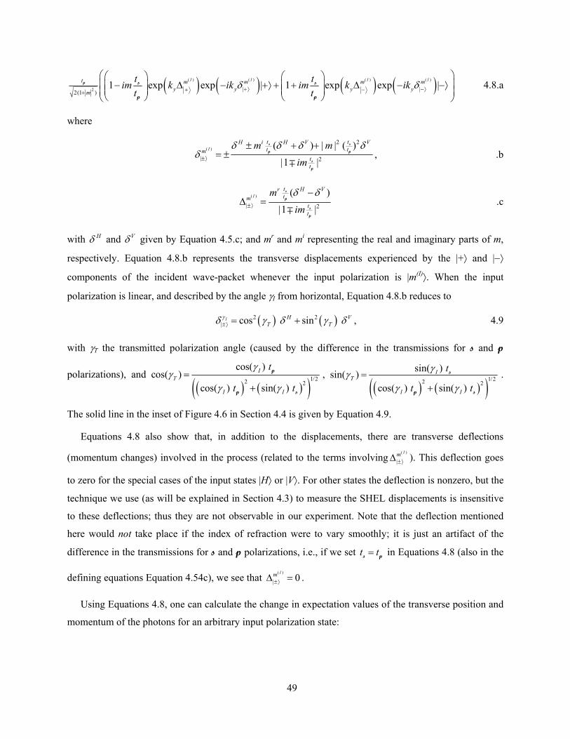
49

( ) ( ) ( ) ( )( ) ( ) ( ) ( )

2 | |2(1 )1 exp exp | 1 exp exp |

I I I It m m m my y y ym

t tim k ik im k ikt t

δ δ+⟩ −⟩+ −+

⎛ ⎞⎛ ⎞ ⎛ ⎞⎜ ⎟− ∆ − +⟩ + + ∆ − −⟩⎜ ⎟ ⎜ ⎟⎜ ⎟ ⎜ ⎟⎜ ⎟⎝ ⎠ ⎝ ⎠⎝ ⎠

p s s

p p

4.8.a

where

( )

2 2

| 2

( ) | | ( )

|1 |I

t tH i H V Vt tm

tt

m m

im

δ δ δ δδ ±⟩

± + += ±

∓

s s

p p

s

p

, .b

( )

| 2

( )

|1 |I

tr H Vtm

tt

m

im

δ δ±⟩

−∆ =

∓

s

p

s

p

.c

with Hδ and Vδ given by Equation 4.5.c; and mr and mi representing the real and imaginary parts of m,

respectively. Equation 4.8.b represents the transverse displacements experienced by the |+⟩ and |−⟩

components of the incident wave-packet whenever the input polarization is |m(I)⟩. When the input

polarization is linear, and described by the angle γI from horizontal, Equation 4.8.b reduces to

( ) ( )2 2| cos sin I H V

T Tγδ γ δ γ δ±⟩ = + , 4.9

with γT the transmitted polarization angle (caused by the difference in the transmissions for s and p

polarizations), and ( ) ( )( )1/22 2

cos( ) cos( )

cos( ) sin( )

IT

I I

t

t t

γγ

γ γ=

+

p

p s

, ( ) ( )( )1/22 2

sin( ) sin( )cos( ) sin( )

IT

I I

t

t t

γγγ γ

=+

s

p s

.

The solid line in the inset of Figure 4.6 in Section 4.4 is given by Equation 4.9.

Equations 4.8 also show that, in addition to the displacements, there are transverse deflections

(momentum changes) involved in the process (related to the terms involving( )

|

Im±⟩∆ ). This deflection goes

to zero for the special cases of the input states |H⟩ or |V⟩. For other states the deflection is nonzero, but the

technique we use (as will be explained in Section 4.3) to measure the SHEL displacements is insensitive

to these deflections; thus they are not observable in our experiment. Note that the deflection mentioned

here would not take place if the index of refraction were to vary smoothly; it is just an artifact of the

difference in the transmissions for s and p polarizations, i.e., if we set t t=s p in Equations 4.8 (also in the

defining equations Equation 4.54c), we see that ( )

| 0Im

±⟩∆ = .

Using Equations 4.8, one can calculate the change in expectation values of the transverse position and

momentum of the photons for an arbitrary input polarization state:

50

( )

( ) ( ) ( )2

2 2 2 2

2 cos ( ) 1 cos( )

1 | | ( ) sin 1 | | ( )

t tti H V i T It ttt t

I It t

m mym k m

θ θδ δ

θ

− ++∆ = =

+ +

s ss

p pp

s s

p p

, 4.10.a

( )2 22

2 2 2 2

4 ( ) 1 ( )cot4

1 | | ( ) 1 | | ( )

t tr H V rkt tI

y kt tIt t

m mk

m k m

δ δ σ θσ

− −∆ = =

+ +

s s

p p

s s

p p

, .b

where 22 2 ( )k y y ydk k kσ ≡ Φ∫ , with the condition that the transverse momentum distribution

2( )ykΦ is

sufficiently centered around 0yk = . These results are in accordance with references 68,69.

4.2.2 Contradicting theories and angular momentum conservation

The expectation value of the spin Hall displacements involved for an arbitrary input polarization state was

calculated in reference 52 by using solely the conservation of total (spin + orbital) angular momentum

around the z-axis, due to the rotational symmetry. However, the results of this calculation (see Equations

4.12) are different than the ones given by Equations 4.10. The predictions of reference 52 were further

verified in reference 67 by solving Maxwell’s equations directly. This section is intended to resolve these

discrepancies.

We will call the physical model (resulting in Equations 4.10) which has been used throughout this

work and verified by our experiment, the “common-polarization” model. On the other hand, we will call

the physical model which gives the results obtained in references 52, 67, the “fixed-polarization” model;

here we investigate some of its physical properties to understand its differences from the “common-

polarization” model. Specifically, we will now show that the input state described by the “fixed-

polarization” model is not representative of that prepared in a typical experiment.

First, we note that a wave-packet incident on an interface at an angle θI is not in an eigenstate of the

angular momentum projection onto the z axis. As a consequence, it is not always possible to calculate the

expectation values of the displacements without first decomposing the incident wave-packet into a set of

eigenstates of the angular momentum projection onto the z axis (since there is also a reflected part of the

wave-packet in addition to the relevant transmitted part (see also the discussion in references 68,69) and

the transmission coefficients for different constituent angular momentum eigenstates may differ from

each other, giving rise to further complications). Nevertheless, there are special input wave-packet states

for which angular momentum conservation for the expectation values straightforwardly yields the correct

displacements. The input wave-packet of the “fixed-polarization” model is a particular example of these

special input states.

51

As illustrated in Figure 4.2, all the wave-vector components of the input wave-packet of the fixed-

polarization model, regardless of their directions, have the same, fixed contributions of s and p

polarizations, as opposed to having a common polarization state. (A common polarization state for all the

wave-vector components indicates that the s or p contributions have to vary as a function of the wave-

vector direction to keep the polarization the same, e.g, see Equations 4.4) For example, an incident wave-

packet in the fixed-polarization model can be completely s- or p-polarized, which is not possible in the

common-polarization model. In practice, however, the wave-packets of the common-polarization model

are the actual physical ones that come out of a polarizer. Only for the peculiar input wave-packet

described by the fixed-polarization model do all the constituent wave-vector components acquire the

same polarization modification due to Fresnel reflections, thereby enabling the displacement calculations

using conservation of angular momentum. The ‘horizontally’ and ‘vertically’ polarized input wave-

packets |Ψ′H⟩ and |Ψ′V⟩ of the fixed-polarization model that are closest to the

( )12

| ( )| | ( )| |H dy y y dy y yΨ ⟩ = Ψ ⟩ +⟩ + Ψ ⟩ −⟩∫ ∫ and ( )2| ( )| | ( )| |i

V dy y y dy y y−Ψ ⟩ = Ψ ⟩ +⟩ − Ψ ⟩ −⟩∫ ∫ input wave-

packets of the common-polarization model can be calculated by superposing the individual wave-vector

components, resulting in ( )( ) ( )12

| ' ( )| | ( )| |I IH dy y y dy y yδ δΨ ⟩ = Ψ − ⟩ +⟩ + Ψ + ⟩ −⟩∫ ∫ and

Figure 4.2: Illustration of the two different polarization models. Red lines represent different wave-vectorcomponents of an input wave-packet. Only three components are shown out of a continuum of wave-vectors. a, In the common-polarization model shown here the polarization vectors associated withindividual wave-vector components are all the same and point along the xI axis. b, In the correspondingfixed-polarization model the polarization vectors associated with individual wave-vector components liein the plane formed by the wave-vector and its projection onto the interface surface (p-polarized), andthus are different from each other. We can also draw the two figures corresponding to the polarizationsthat are orthogonal to the ones shown here. In that case the analog of part a will have its polarizationvectors in the plane formed by the zI and y axes, such that the polarization vectors are perpendicular to thewave-vectors, and the analog of part b will have its polarization vectors perpendicular to the plane formedby the wave-vector and its projection onto the interface surface, i.e., corresponding to s-polarized light.

52

( )( ) ( )2

| ' ( )| | ( )| |I IiV dy y y dy y yδ δ−Ψ ⟩ = Ψ − ⟩ +⟩ − Ψ + ⟩ −⟩∫ ∫ . We see that the input wave-packets in the fixed-

polarization model are already split (in |+⟩ and |−⟩ wave-packets) in the y-direction before the spin Hall

effect takes place at the interface. Here ( )( ) cotII Ikδ θ= , indicating that the separation between the |+⟩

and |−⟩ states in the input wave-packet is different for different incidence angles. These are rather unusual

initial conditions, not representative of those prepared in a typical experiment. Notice that the

displacement ( )Iδ diverges as the input wave-packet approaches normal incidence. The position space

description we have presented here is only valid in the regime when ( )Iδ is much smaller than the

transverse wave-packet size. For larger ( )Iδ there is also beam distortion, i.e., the initial separation

between wave-packets corresponding to |+⟩ and |−⟩ states can never be larger than the wave-packet size.

Nevertheless, the spin Hall displacements that we will calculate now for the fixed-polarization model will

be valid for all incidence angles. Furthermore, we will show that this model reproduces the results of

references 52 and 67.

The positions for the |+⟩ and |−⟩ states for the transmitted wave-packet in the fixed-polarization model

are determined by ( ) ( )( )( ) cos sinTT I Ikδ θ θ= . Therefore, the displacements caused by the SHEL in this

model are given by:

( ) ( )( )

( ) ( )|

cos cos2 sin

T IT I

I

θ θλδ δ δπ θ±⟩

−∆ = − = ± . 4.11

Equation 4.11 is to be compared with Equation 4.1, which gives the displacements according to the

common-polarization model. Note that, in the fixed-polarization model (Equation 4.11), the

displacements in the |+⟩ and |−⟩ states are independent of the input polarization state. The displacements

predicted by the various models discussed here are displayed in Figure 4.3.

The “fixed-polarization” model developed here can be easily shown to reproduce the results of

references 52 and 67 by calculating the expectation values of the displacements ( ) ( )T Iy y y∆ = − due

to the SHEL for a general input polarization state ( )2

( ) 11 | |

| ' | ' | 'I

mm H m V

+⟩ = ⟩ + ⟩ . With the expectation

values ( )Iy and ( )Ty given by ( )

( )21 | |

i II my

mδ

=+

and ( )

( )2 2

2

1 | | ( )

ti TtT

tt

my

m

δ=

+

s

p

s

p

, we obtain:

53

( )

( ) ( )2 22

cos cos2sin 1 ( ) 1

tiTt It

I I t

myk m m

θ θθ

⎛ ⎞⎜ ⎟∆ = −⎜ ⎟+ +⎝ ⎠

s

p

s

p

, 4.12.a

0yk∆ = . .b

Equations 4.12 are the same as the results obtained in references 52 and 67.

We would like to note that if the interface is perfectly anti-reflection coated, such that / 1t t →s p , both

of the models are expected to give the same result for the amount of SHEL displacements.

Figure 4.3: Comparison of different theories. |δH| and |δV| are determined by Equation 4.1.|∆δ | = δ (T) - δ (I) is given by Equation 4.11. The predictions are for incident photons with wavelength λ =633 nm and n=1.515. In the model resulting in Equation 4.11, the wave-packets associated with the twospin components are initially (before the interface) displaced in opposite directions by ±δ (I). After theinterface the displacements become ±δ (T). The difference in the positions before and after the interfacereveals the displacements |∆δ | due to the SHEL. Notice that |∆δ | is close (but not identical) to theaverage of |δH| and |δV| predicted by the common-polarization model resulting in Equation 4.1.

54

4.3 Weak measurements as a metrological tool

For optical wavelengths, precise characterization of the displacements involved in the SHEL requires

measurement sensitivities at the Angstrom level. To achieve this sensitivity we use a signal-enhancement

technique known from quantum weak measurements [5]. As introduced in Section 1.1, in a quantum

measurement, a property (observable A ) of a system is first coupled to a separate degree of freedom (the

‘meter’), and then the information about the state of the observable is read out from the ‘meter’. At the

single-photon level, the SHEL is actually equivalent to a quantum measurement of the spin projection

along the central propagation direction (observable 3σ , with eigenstates |+⟩ and |–⟩), with the transverse

spatial distribution serving as the ‘meter’ (similar to the Stern-Gerlach spin projection measurement

discussed in Section 1.1, but here, the principal observable of the ‘meter’ is the position, as opposed to

momentum). However, the displacements generated by the SHEL here are much smaller than the width of

the transverse distribution, resulting in a weak measurement (satisfying the criteria introduced in Section

1.2): the ‘meter’ states associated with different spin eigenstates overlap to a large extent. Therefore, the

‘meter’ carries very little information about the state of the observable, leaving the initial state almost

undisturbed. Here we stress that although our experiment is at a classical level with a large number of

photons in a quantum mechanical coherent state, the results remain the same, each photon behaving

independently. Furthermore, in the paraxial regime the dynamics of the transverse distribution is given by

the Schrödinger equation with time replaced by path length, making the analysis identical to non-

relativistic quantum mechanics (as will be discussed further in Section 4.3.1) with an impulsive

measurement interaction Hamiltonian ˆˆ ( )I yH g t k δ= A . Here, impulsive means that g(t) is given by a

Dirac delta-function.

The signal enhancement technique uses an appropriate pre- and post-selection (PPS) of the state of the

observable. As described in Section 1.2, a weak measurement with PPS is basically a conditional weak

measurement of a ‘system’ that is initially in state |ψ1⟩. Specifically one reads out the ‘meter’ only if the

state of the ‘system’ is found to be in state |ψ2⟩ after a subsequent strong measurement (i.e., the post-

selection). With the PPS, the signal enhancement technique achieves an enhanced displacement in the

‘meter’ distribution [5,79] (Figure 4.4.a). Given the PPS states |ψ1⟩ and |ψ2⟩, for sufficiently weak

measurement strengths, the final position of the ‘meter’ is proportional to the real part of the so-called

‘weak value’ of the measured observable A , introduced in Section 1.2:

2 1

2 1

ˆ| ||wA ψ ψ

ψ ψ⟨ ⟩

=⟨ ⟩

A , 4.13

55

which increases as the post-selected state approaches being orthogonal to the pre-selected one (since the

denominator becomes small). This effect was previously demonstrated [80] as a factor of 20 enhancement

of a birefringent displacement of photons, in which the weak value was real. The imaginary part of a

weak value corresponds to a displacement in the momentum-space distribution of the ‘meter’, which with

free evolution leads to the possibility of even larger enhancements. Furthermore, the order does not

matter: the free evolution can take place first, followed by the weak measurement, but the final

displacement will be identical (Figure 4.4.b). We describe the final displacement of the ‘meter’ as the

‘modified weak value’, modw wA F A= , where the factor F depends on the initial state of the ‘meter’ and

the amount of its free evolution before detection. The details are described in the following section.

4.3.1 The modified weak value

In this section we show that a weak measurement of an observable A in the presence of PPS yields the

weak value Aw of that observable. Following that, we concentrate on the case of an imaginary weak value

and derive what we call the “modified weak value” modwA of an observable, together with the connection

to our experimental setup. Here we clarify that the development of the weak measurement technique was

historically guided by quantum mechanics; nevertheless, the results still apply at the classical level (as in

Figure 4.4: A weak quantum measurement with PPS. a, System starts in state |ψ1⟩. The measurementinteraction weakly correlates the meter with the eigenstates of the measured observable A . A post-selection on the system in state |ψ2⟩ gives rise to an interference in the meter, shifting its final positionproportional to Aw (Equation 4.13). b, When Aw is imaginary, modifying the state of the meter by meansof a free evolution (either before or after the weak measurement of A ; before is shown here) makes thefinal meter position proportional to Aw

mod , which can be much larger than Aw.

56

our experiment) as long as the meter is not a separate particle, but instead a different degree of freedom of

the particle that is being measured. Also note that if our experiment were to be carried out at the quantum

level (with single photons), the results would have been identical, since the classical level corresponds to

nothing but a large number of independent photons in a quantum mechanical coherent state. Put

differently, the first-order quantum interference effects described below survive the “correspondence

principle” limit to the classical level.

In a quantum measurement, an observable of a system is first coupled to a meter (be it another particle

or a separate degree of freedom of the very same particle), and then the meter is read out, from which

information about the observable is acquired. The initial state is given by

1 1| ( )| | ( )| |initial y y yΨ dy y y dk k kψ ψ⟩ = Ψ ⟩ ⟩ = Φ ⟩ ⟩∫ ∫ , in the position and momentum representations of the

meter, respectively. Here 1| |i ii

c aψ ⟩ = ⟩∑ is the pre-selected state of the system, with ci being the

expansion coefficients, and |ai⟩ the eigenstates of the observable A : ˆ | |i i ia a a⟩ = ⟩A . The system and meter

evolve under the interaction Hamiltonian ˆˆ ( )I yH g t k δ= A . This Hamiltonian couples the momentum of

the meter to the observable A , propagating the initial state |Ψinitial⟩ forward in time as

( )0

ˆ| | ' exp ' ( ') / |

t

initial I initialtΨ Ψ i dt H t Ψ⟩ → ⟩ = − ⟩∫ , entangling the meter states with eigenstates |ai⟩:

( )| ' ( )exp | | ( )| |i y y y i y i i i ii i

Ψ c dk k ik a k a c dy y a y aδ δ⟩ = Φ − ⟩ ⟩ = Ψ − ⟩ ⟩∑ ∑∫ ∫ (with g(t) being given by a Dirac

delta-function, 0

ˆ ˆ' ( ') /

t

I ytdt H t k δ=∫ A ). In the case of a strong measurement, the meter states

corresponding to different observable states become completely separated. However, for a weak

measurement, these states overlap significantly (that is, aiδ are much smaller than the initial width of the

meter state), and we can treat the operator ( )ˆexp yik δ− A perturbatively, expanding it as ˆ1 yik δ− A .

Therefore, 1 1ˆ| ' ( )| | ( ) | |y y y y y y yΨ dk k k i dk k k kψ δ ψ⟩ ≅ Φ ⟩ ⟩ − Φ ⟩ ⟩∫ ∫ A . If we make a post-selection in state ⟨ψ2|,

the reduced state of the meter becomes:

( ) ( ) ( )2 2 1 2 1| ' | exp | | |y y y w y wΨ dk k ik A k dy y A yψ ψ ψ δ ψ ψ δ⟨ ⟩ = ⟨ ⟩ Φ − ⟩ = ⟨ ⟩ Ψ − ⟩∫ ∫ , 4.14.a

with

2 1

2 1

ˆ| ||wA ψ ψ

ψ ψ⟨ ⟩

=⟨ ⟩

A . .b

57

If the weak value Aw is real, the meter shifts to a final position proportional to Aw. On the other hand, if

Aw is imaginary, the momentum distribution of the meter is altered from Φ(ky) to ( )1 ( )y w yk A kδ+ Φ (to

first order in δ). For certain Φ(ky) that are symmetric about 0yk = , e.g., a Gaussian Φ(ky), this is simply

equivalent to a displacement of the momentum distribution. For a general state, the effect is more than

just a simple displacement of the momentum distribution, but can be expressed as a shift in the

expectation values yk and y , determined by the particular form of Φ(ky). Here we concentrate on the

particular case used in our experiment. Assume that we start (at the location of the beam waist) with an

initial momentum wavefunction Φ0(ky) which is real, and let it evolve with the free Hamiltonian of the

meter (the kinetic energy term 2

2ypm with y yp k= ) : ( )2

0 0 2( ) ( ) ( )exp ypy y y mk k k i tΦ → Φ = Φ − . As applied to

our experiment, in the paraxial approximation (e.g., see Section 2.2.C of reference 81), time t is replaced

by an effective propagation distance zeff (optical path length), and the mass m is effectively replaced by

the central wave-vector along the propagation direction of the wave-packet:

( ) ( )2 2

2 2exp expy y

I

p keffm ki t i z− ↔ − . Including the weak measurement and PPS, the momentum wavefunction

then becomes:

( ) ( )2

0 0( ) 1 ( )exp2

yy y y w y eff

I

kk k k A k i z

kδ

⎛ ⎞Φ → Φ = + Φ −⎜ ⎟⎜ ⎟

⎝ ⎠. 4.15

Given that 0y = and 0yk = for the initial meter state Φ0(ky), we can calculate y for the

modified state in Equation 4.15 (for a purely imaginary Aw) as:

2 22 2eff y I mod

w w wI eff

z k k yy A A A

k zδ δ δ= = = , 4.16

where we have used the fact that the width of the position distribution of the beam after free evolution

(this width is much larger than its value at the beam waist) can be expressed in terms of the momentum

spread: 2

2 22

effy

I

zy k

k≅ . Here, mod

w wA F A= with 2 22 4I

eff eff

k y yF

z zπ

λ= = . If one assumes that the weak

measurement and post-selection are instantaneously performed when the meter state was Φ′(ky), then the

interpretation would be that these steps shifted the momentum distribution, and with the free propagation

the wave-packet moved to its final position y given by Equation 4.16. However, the free propagation

commutes with the weak measurement and the PPS; therefore, even if the free propagation takes place

58

first, followed by the weak measurement and post-selection, the final y value remains the same. In the

latter case the interpretation would be that due to an interference effect the post-selection shifted the

position to y as given by Equation 4.16. The bottom line is that the beam displacement at a distance zeff

from the beam waist turns out to be independent of the position of the weak measurement and the PPS.

For our experiment (Figure 4.5), this means that the exact location of the prism (where the SHEL takes

place) and the polarizers (where the PPSs take place) does not affect the measured displacements.

4.4 The experiment

In our experiment (Figure 4.5), the SHEL takes place at the front surface of a variable angle prism (VAP)

for various incidence angles θI, with the back surface adjusted to be at normal incidence to avoid

secondary Hall shifts (as there is obviously no Hall shift at normal incidence). The VAP is constructed by

attaching two BK7 round wedge prisms together with the surface tension of a thin layer of index-

matching fluid, and is mounted loosely to avoid any stress-induced birefringence. The prisms can rotate

with respect to each other, and the entire assembly can rotate around three orthogonal axes, allowing the

desired surface orientations. The enhancement effect that has been described in Section 4.3 is achieved by

the PPS of the polarization states of the incoming photons in states |ψ1⟩ and |ψ2⟩, by the calcite polarizers

P1 and P2, respectively:

( )11| | | |2

Hψ ⟩ = ⟩ = +⟩+ −⟩ , ( ) ( )( )21| | exp | exp |2

V i i i iψ ⟩ = ± ∆⟩ = − ∆ +⟩ + ± ∆ −⟩∓ . 4.17

1∆ being a small angle, the weak value of the spin component is given by: ( )3ˆ cotw

i iσ = ∆ ≈ ∆∓ ∓ .

Lenses L1 and L2 focus and collimate the transverse spatial distribution of the incoming photons. The

factor F in the modified weak value is determined by the transverse spatial state of the photons after lens

L2, and as derived in Section 4.3.1, it is given by:

2

24 L

eff

yF

zπ

λ= . 4.18

Here 22Ly is the variance of the y-direction transverse distribution after lens L2, and 125 5effz = ± mm is

the effective focal length of L2. The design of the VAP ensures that the optical path length inside of the

VAP remains the same for all incidence angles (assuming the beam is centered on the entrance surface),

so that F is always the same. We achieve a displacement at the position sensor (PS) by an amount that is

3ˆ( ) cotmodw F Fσ = ∆ ≈ ∆∓ ∓ times larger (~104 for our system) than the displacement caused by the SHEL

59

alone, and we measure this by reading out25 the difference between the displacements for the two post-

selections |V±∆⟩. These post-selections are accomplished by mechanically rotating the polarizer P2. As

stressed in Section 4.3.1, the exact location of the VAP and the polarizers do not affect the measured

displacements. Similarly, the exact location of the PS does not make a difference either, due to the chosen

location of L2.

The results are presented in Figure 4.6. The dotted lines, which overlap with the solid lines up to 64°,

represent the theory with the photons exiting the prism at normal incidence (Equation 4.1). The solid lines

also take into account the modifications (described and derived in Section B.1) arising from the fact that

our VAP cannot satisfy the normal exiting condition beyond 64°. In order to stay in the linear response

regime of both the enhancement technique and the PS, for incidence angles larger than 56° the

enhancement is adjusted (through the polarizer angle ∆) to be lower by a factor of 1.8: 3ˆ| ( ) | 57.3 0.7wσ = ±

for θI≤56°, 3ˆ| ( ) | 31.8 0.2wσ = ± for θI>56°, corresponding to post-selection polarizer angles of 1∆ = ±

and 1.8∆ = ± , respectively. With the value of F determined from a single-parameter fit to be 156 2± , all

the data points lie on the theoretical curves (Figure 4.6) with a standard deviation of 3.5Å from the theory

25 The position measurements are carried out using a position sensitive detector, in particular a Pacific Silicon

Sensor Inc. quad-cell with integrated pre-amplifier circuitry. An OP27 op-amp based custom circuit was built for another stage of amplification (~103 variable amplification) and a following AD734 multiplier/divider chip based circuit was built for intensity normalization before read-out by a multi-meter or an oscilloscope. Note that a quad-cell is a split-photodiode with four quadrants, and it utilizes position measurements, e.g. by signaling the intensity difference between the right and left quadrant pairs (or up and down pairs). More information relevant to the amplification and normalization circuits can be found in reference 132.

Figure 4.5: Experimental setup for characterizing the spin Hall effect of light. The light source is a 10-mW linearly polarized He-Ne laser at 633 nm. VAP: variable angle prism (material: BK7, refractiveindex n=1.515 at 633 nm), P1 & P2: Glan Laser polarizers, L1 & L2: Lenses with effective focal lengths25 mm and 125 mm, PS: position sensor (a split photodiode), HWP: half-wave plate (for adjusting theintensity after P1).

60

(excluding the last two data points of curve |δ H|, where there is a small, as yet unexplained, discrepancy).

By measuring 22Ly , we can also experimentally determine the value of F, albeit less accurately; we find

157 6± , indicating the total enhancement factor to be ( ) 33ˆ( ) 8.97 0.36 10mod

wσ = ± × for θI≤56° and

( ) 33ˆ( ) 4.99 0.20 10mod

wσ = ± × for θI>56°. Sources of noise and uncertainty will be discussed in the next

section.

Figure 4.6 also shows the dependence of the displacements on the incident linear polarization (see

Section 4.2.1 for the theory). As derived in Section 4.2.1, note that for arbitrary incident polarization

(other than |H⟩ or |V⟩), a kick in the y-momentum is also expected; however, the magnitude of the kick is

the same for the constituent |R⟩ or |L⟩ components of the wave-packet. Since there is no relative change,

our measurements are insensitive to this effect.

Figure 4.6: Experimental results for the magnitude of the opposite shifts of the two spin components as afunction of incidence angle. The |δ H| (|δ V|) data sets are half the measured separation between the twospin components for horizontal (vertical) incident polarization. The error bars represent two standarddeviations. Dotted lines: Theory (Equation 4.1), solid lines: modified theory, accounting for secondaryHall shifts at the exit surface of the prism (Equation B.3). The inset shows the results as a function ofincident polarization angle for a fixed incidence angle of 64°.

61

4.5 Conclusions

The measurability of very small displacements is ultimately limited by the quantum noise of the light, as

enough photons need to be collected to resolve the position of the transverse distribution [82]. In the

absence of any focusing or expansion of the beam, i.e., when F = 1, if the experiment is already quantum-

noise limited, then for a fixed number of photons entering the experimental setup, the enhancement due to

PPS does not bring any gain in the measurement sensitivity: although the displacement is multiplied by a

factor of 3ˆ( ) 1wσ ≈ ∆ , only a fraction of the photons ( 2 2 21 2| sinψ ψ⟨ ⟩ = ∆ ≈ ∆ ) make it through the post-

selection, which cancels the advantage of the enhancement. Nevertheless, most experiments are limited

by technical issues, e.g., in our setup, the laser pointing stability, the intensity saturation of the PS, or the

unwanted (~10 µm) displacements caused by rotating the polarizers. Note that all of the technical noise

mentioned here creates an electrical signal that is linear in the intensity of the light incident on the PS, i.e.,

proportional to ∆2. On the other hand, the electrical signal due to the actual displacements after the

enhancement technique is proportional to ∆. Therefore, despite the overall loss in the signal as ∆ becomes

smaller, the SNR increases.

The beam focusing and expansion, leading to F > 1, also increases the SNR for the case of technical

noise mentioned above (by a factor of F), but without an overall decrease in the signal. The latter is true

because the displacements are enhanced by a factor of F while the electrical signal from the PS is reduced

by a factor of F since the electrical signal is inversely proportional to the beam area for a given incident

power. Note that the displacement enhancement technique eliminates the requirement of going to smaller

and smaller beam sizes to make more and more accurate measurements of the displacements. There are

two ways of thinking about the quantum noise for the case of F > 1. For a given number of incident

photons, the quantum noise on the position of a beam at the PS for F > 1 is F times larger in comparison

to the case of F = 1. However, the original displacements, say δ, are F times larger as well (i.e., Fδ).

Thus, the technique provides no loss or gain in the SNR for quantum noise. On the other hand, using the

measured displacements we are actually inferring the magnitude of the F-fold smaller original

displacements δ, but with the ease of using a large beam. From this perspective, the inferred

displacements are a factor of F below the standard quantum limit.

In or experiment, we suppress technical noise by a factor of 43ˆ( ) 10mod

wσ ≈ with respect to the signal,

and achieve a sensitivity/stability to displacements of ~1Å, without the need for vibration or air-

convection isolation. The upper limit to the enhancement comes from the achievable extinction ratio of

the polarizers and from the electronic noise in the PS. As we will see in Section 5.2, with the use of

62

time-varying post-selection and lock-in detection techniques, the resolution can be increased by almost

two orders of magnitude.

The weak measurement enhancement techniques used for the first time in this work have inspired

other groups as well, for example, to measure the SHEL upon reflection from a surface [83], or to make

ultrasensitive beam deflection measurements [84,85], for eventual use in detection of gravitational red-

shift, with slow light [86].

Spin Hall displacements can be made arbitrarily large, in principle, separating beams associated with

different spin states simply by cyclic motion or with the aid of periodically modulated media [52,74,87].

This may prove useful for potential applications requiring the complete separation of different spin

components. An orbital version of the effect, which can separate different orbital angular momentum

states, was also suggested [75]; however, it was realized later that the beam structure was distorted in the

process [88] (causing scattering into different orbital angular eigenstates), preventing its use for the

purpose of separation of the eigenstates. The SHEL itself may prove to be an advantageous metrological

tool, e.g., for characterization of photonic structures, or for characterizing refractive index variations

measured at sub-wavelength distances from the region of interest, since any Hall displacement

accompanying a beam deflection is larger than the displacement caused by the deflection itself at such

propagation distances. Another potential application could be in astronomy, where received images could

be analyzed in the R- and L-polarization basis for any displacements due to SHEL; information on the

actual location of the object could be gained, for example, if the light had encountered any bending due to

gravity or matter-density gradients on its way to the telescope.

63

Chapter 5 Spin Hall Effect of Light – II: Smooth index variations

In the previous chapter, we have investigated the SHEL at an air-glass interface, and saw that Fresnel

reflection at the boundary between the two media introduces additional complications. As we will see in

this chapter, for a beam of light traveling in a medium with a smoothly-varying index of refraction, the

SHEL takes a more simple and elegant form. The basic principle remains still the same (i.e., the spin-

dependent transverse displacements), however, the input polarization dependence of the splitting between

the two spin components disappear. In addition, the theoretical description takes a very interesting form,

and reveals interesting connections to other fundamental theories of physics. In particular the equations of

motion can be described as that of a quantum particle moving in the presence of a vector potential in

momentum-space (as opposed to real-space; e.g., as in the case of electrodynamics), which gives rise to a

magnetic field in momentum-space whose form is that of a magnetic monopole.

We will derive the theory behind the effect in Section 5.1. The derivation given can be thought as

complementary to references 87,89. A treatise on the general subject of spin gauge fields can be found in

reference 90. We will describe our experiment for the case of smooth index variations in Section 5.2 in

conjunction with the use of time-dependent post-selection techniques to achieve better resolutions.

5.1 Theory: Smoothly varying index of refraction

Arguably, the most fundamental equations in physics (along with the Dirac equation describing fermions)

are the Maxwell’s equations describing electromagnetic waves. These equations in continuous media, in

the absence of free charges and currents, take the vector form [91]:

0⋅ =D∇ 5.1.a

t

∂= −

∂B

∇ × Ε .b

t

∂=

∂D

∇ × Η .c

0⋅ =B∇ . .d

64

For linear, isotropic but inhomogeneous media, the electric displacement vector D is given in terms of

the electric field vector E by D = ε(r) E, with ε(r) being the position-dependent permittivity of the

medium26. Since the magnetic response of common optical materials is negligible, for optical frequencies,

the magnetic field B is given in terms of the magnetic field intensity H by B = H µ0 , with µ0 being the

permeability of free space. Alternatively, in the matrix form more commonly used in relativistic quantum

mechanics, Equations 5.1.b&c take the forms 0( ) E Hti µ ∂∂⋅ − = −T ∇ and ( ) H ( ) E ti ε ∂

∂⋅ − =T r∇ ,

respectively. Here, an underscore represents a column vector, and a double underscore represents a

matrix. Note that –i ∇ is the familiar momentum operator in quantum mechanics (up to a factor of ).

The T appearing in the equations is a vector matrix, where component matrices are the generators of

rotation in three dimensions, the SO(3) group27.

26 Note also that ε(r) = ε0 εr(r) = ε0 n2(r), where ε0 is the permittivity of free space, εr(r) is the relative

permittivity, and n(r) is the refractive index of the medium. In addition, εr(r) = 1+χ(r), with χ(r) being the electric susceptibility of the medium. Also, µ0 ε0 = 1/c2, with c being the speed of light in vacuum.

27 If we adopt the representation 2

3

1

EEEE

⎛ ⎞⎜ ⎟≡ ⎜ ⎟⎜ ⎟⎝ ⎠

, with the basis vectors

0|1 0

1

⎛ ⎞⎜ ⎟⟩ ≡ ⎜ ⎟⎜ ⎟⎝ ⎠

,

1|2 0

0

⎛ ⎞⎜ ⎟⟩ ≡ ⎜ ⎟⎜ ⎟⎝ ⎠

,

0|3 1

0

⎛ ⎞⎜ ⎟⟩ ≡ ⎜ ⎟⎜ ⎟⎝ ⎠

, the

generators take the form: 1

0 0T 0 0

0 0 0

ii

−⎛ ⎞⎜ ⎟= ⎜ ⎟⎜ ⎟⎝ ⎠

, 2

0 0 0T 0 0

0 0i

i

⎛ ⎞⎜ ⎟= −⎜ ⎟⎜ ⎟⎝ ⎠

, 3

0 0T 0 0 0

0 0

i

i

⎛ ⎞⎜ ⎟= ⎜ ⎟⎜ ⎟−⎝ ⎠

. In terms of these matrices, the

cross-product operator is represented as ( ) Bi≡ − ⋅A×B T A . The T matrices are represented in the linear polarization basis. One can transform into the circular polarization (or spin) basis with the aid of the unitary operator

2

1 01U 0 02

1 0

ii

i

⎛ ⎞⎜ ⎟= −⎜ ⎟⎜ ⎟−⎝ ⎠

and its adjoint †2

1 0 11U 0 02

0i

i i

⎛ ⎞⎜ ⎟= ⎜ ⎟⎜ ⎟−⎝ ⎠

: 1

0 1 01S 1 0 12

0 1 0

⎛ ⎞⎜ ⎟= ⎜ ⎟⎜ ⎟⎝ ⎠

, 2

0 01S 02

0 0

ii i

i

−⎛ ⎞⎜ ⎟= −⎜ ⎟⎜ ⎟⎝ ⎠

,

3

1 0 0S 0 0 0

0 0 1

⎛ ⎞⎜ ⎟= ⎜ ⎟⎜ ⎟−⎝ ⎠

with the transformation rule †S U T Ui i= . Notice that these matrices are the familiar spin-1

matrices in quantum mechanics. The new basis vectors in the spin representation are given in terms of the original basis vectors, by ( )† 1

2| U |2 |1 |2i+⟩ = ⟩ = − ⟩ + ⟩ , ( )† 1

2| U |1 |1 |2i−⟩ = ⟩ = ⟩ + ⟩ , †|0 U |3 |3i⟩ = ⟩ = ⟩ . Note that

3S | 1|±⟩ = ± ±⟩ and 3S |0 0 |0⟩ = ⟩ . In order to be consistent with the other sections, one can define the horizontal polarization as | |2H ⟩ = ⟩ , and the vertical polarization as | |1V ⟩ = − ⟩ . Both the T and the S matrices satisfy the commutation relations of an angular momentum operator: [T ,T ] Ti j ijk kiε= and [S ,S ] Si j ijk kiε= , with εijk being the

totally anti-symmetric tensor. In the spin basis Maxwell’s Equations 5.1.b&c become 0ˆ E Hs stµ ∂∂⋅ = −S p and

ˆ H ( ) Es stε ∂∂⋅ =S p r . The subscript ‘s’ is there to remind that the column vectors are in the spin representation,

and is inserted for convenience, in order to use the momentum operator ˆ i≡ −p ∇ .

65

Maxwell’s Equations 5.1.b&c can be put together to result in a wave equation for the electric field

function. In matrix form the wave equation then reads:

2

0 2( ) ( ) E( , ) ( ) E( , ) 0i i t tt

µ ε ∂⋅ − ⋅ − + =

∂T T r r r∇ ∇ . 5.2

For a monochromatic field of angular frequency ω, this equation becomes (with ω2 = k02 c2 ):

20( ) ( ) E( , ) ( ) E( , ) 0ri i t k tε⋅ − ⋅ − − =T T r r r∇ ∇ . 5.3

Due to the first term, this equation is non-diagonal, and causes a coupling between the different

components of the electric field function column vector. Maxwell’s Equation 5.1.a states that there are

only two independent components of the electric field, and in the absence of a spatially varying

permittivity, the electric field is strictly transverse. This suggests that perhaps in the presence of a

variation in the permittivity, provided that the variation is slow, one can to a good approximation

diagonalize Equation 5.3 by defining a new basis set for the electric field vector that varies from point to

point in space, such that, for instance, the third component of the basis set is always in the direction of the

local propagation direction28 (as shown pictorially in Figure 5.1.a). Then, to a good approximation this

third component will drop out of the equations since it is practically not occupied.

Mathematically this diagonalization is most easily accomplished in momentum-space (or wave-vector-

space). Defining 3/23 1

(2 )E( , ) ( , ) exp( )t d k t i

π

∞

−∞= ⋅∫r k k rE and 3/2

3 1(2 )

( , ) E( , ) exp( )t d r t iπ

∞

−∞= − ⋅∫k r k rE ,

Equation 5.3 in momentum-space (with k being the wave-vector, and ∇k being the gradient operator in

momentum-space) reads29:

20 ( , ) ( ) ( , ) 0rt k i tε⋅ ⋅ − =kT k T k k k ∇E E . 5.4

Diagonalization can be accomplished by transforming Equation 5.4 with the unitary rotation operator

ˆ ˆR ( ) exp( n )iθ θ= − ⋅n T with an appropriate selection of the unit vector n and rotation angle θ., such that

the third component of the polarization basis vector will coincide with the direction of the wave-vector as

shown Figure 5.1.b. Note that n and θ are functions of k. The resulting wave equation is30:

28 Note that this turns out to be equivalent to finding the eigenstates of the operator ( )i⋅ − ≡ ⋅T T k∇ , with k

being the wave-vector. 29 Since E( , )tr is real, it must follow that *( , ) ( , )t t= −k kE E . 30 2 2

ˆ ˆ ˆ ˆ ˆR ( ) exp( n ) [1 ( n) ] ( n) cos( ) n sin( )i iθ θ θ θ= − ⋅ = − ⋅ + ⋅ − ⋅n T T T T acting on a column vector produces

rotations about the unit vector n by an angle θ. The rotation shown in Figure 5.1.b is best carried out in spherical polar coordinates with ˆn ≡ φ , the unit vector associated with the coordinate φ, and θ is the actual polar coordinate.

66

( )2 2 23 0T ' ( ) ' 0rk k iε− + =k A k ∇E E 5.5

with ' U =E E and †( ) U( U )i= kA k ∇ . Note that this procedure brings the first term into a diagonal form

at the expense of introducing a matrix correction ( )A k to the gradient operator in momentum space,

since U does not commute with the gradient operator. The term 1 1 2 2 3 3( ) T T T= + +A k A A A is a gauge

potential (a vector potential, or sometimes called a connection), and in particular it is a non-abelian one

Then, the unitary operator is ˆU R ( )θφ

= − with †U U 1= . The transformation of Equation 5.4 is accomplished by

multiplying from the left with U, and inserting the identity operator †U U between multiplicative terms: † † 2 †

0U U U U U U ( )U U 0rk iε⋅ ⋅ − =kT k T k ∇E E . Here, we get †3U U T k⋅ =T k , and the calculation of

†U ( )U ( )i fε k k∇ can be done with a Taylor expansion of the function ε: 1'! ' 0

0( ) ( ) ( ')n

nn

i iε ε∞

==

= ⋅∑k k r rr∇ ∇ ∇ ,

with r′ being an auxiliary variable. Note that f(k) is there just to remind that the operator ∇k is actually acting on some function. If we observe the fact that ( )† †U U ( ) U( U ) ( )i f i i f= +k k kk k∇ ∇ ∇ , we get

( )† †U ( )U U( U )i i iε ε≡ +k k k∇ ∇ ∇ . Finally, ˆ ˆ ˆ ˆsin( ) cos( ) cos( ) sin( ) cos( ) 1†

1 2 3sin( )ˆU( U ) T T Tk k ki φ φ φ φ θ

θθ+ φ θ φ −= − + + φk

−∇ .

Figure 5.1: Pictorial representation of defining a new polarization basis set that depends on the localpropagation direction. a, A two-dimensional picture for the new polarization basis set. For simplicity,assume that the waves are uniform in the dimension that is perpendicular to the plane of the page. Theinitial basis set is such that ‘2’ and ‘3’ are aligned with the ‘y’ and ‘z’ axes, respectively, everywhere(globally). The new basis set that is shown is defined at each point (locally) such that the thirdpolarization component is perpendicular to the wave-fronts. This is an approximate description for theexact mathematical implementation given in the text. b, A particular implementation of thetransformation from the old basis set to the new one in three dimensions. The initial polarization basis set,shown in red axes, is initially aligned with the axes of the coordinate frame, shown in black axes. Thetransformation will rotate the red axes by an angle θ about the unit vector n such that the thirdcomponent of the basis set is aligned with the wave-vector k. Here, the use of spherical polar coordinatesis adopted.

67

(i.e., it is a matrix, it is non-diagonal, and when decomposed into generators T1, T2 and T3, the

components do not commute). Note that ( )A k is not unique; e.g., an appropriate rotation about axis-3

followed by a rotation about axis-1 in Figure 5.1.b can equally well align the third component of the

polarization basis vector with the wave-vector. In this case, however, the final orientation of the first and

the second basis components will be different than the previous case, resulting in a different expression

for all components of ( )A k . The choice of aligning one of the three polarization basis vectors with the

wave-vector still leaves us with the freedom to choose the orientation of the remaining two basis vectors

by a rotation about the wave-vector. Thus the alignment breaks the SO(3) symmetry into SO(2), the group

of rotations in a plane (equivalently U(1) symmetry, if one chooses to use complex numbers). This

freedom is precisely the U(1) gauge invariance. With the choice of a gauge, one can have different vector

potentials; nevertheless, the physics described cannot change with different choices of basis vector

orientations.

The T1 and T2 generators couple the third polarization component to the other two components, so

Equation 5.5 is still non-diagonal. However, provided that the relative variations in the permittivity are

small at length scales much larger than the wavelength, it can be shown that the occupation of the third

polarization component is negligible and also that the T1 and T2 components of the gauge potential can be

ignored, with the lowest-order corrections coming from the T3 component. This simplification removes

the third component from the picture, leaving us two components to deal with. The relevant two

components of this equation can also be written using the two-dimensional Pauli matrices:

( )2 20 2 ( )'' '' 0rk k iε σ− − =k kA ∇E E , 5.6

where, the matrix σ2 is the second Pauli matrix (as in Footnote 2 on page 2), and A(k) ≡ A3(k). The

column vector ''E contains the two transverse components made up from the upper and lower components

of 'E (by removing the longitudinal component). At this stage the Equation 5.6 is represented in linear

polarization basis, and still is not completely diagonal. Nevertheless, it will be diagonal once expressed in

circular polarization (or spin) basis, leaving us with two decoupled equations, written in momentum- and

position-spaces, respectively31:

31 Equation 5.6 can be transformed into the spin basis via the unitary operator 1112s

iU

i⎛ ⎞

= ⎜ ⎟−⎝ ⎠. The new field

is defined by '' ''s sU=E E .

68

( )2 20 3 ( )'' '' 0s r sk k iε σ− + =k kA ∇E E 5.7.a

( )2 20 3 ( )Ε'' Ε'' 0s r sk iε σ−∇ − + − =r A ∇ .b

cos( ) 1 ˆ( )sin( )k

θθ−

=A k φ .c

Note that the matrix σ3 is the diagonal Pauli matrix. Thus, within the approximations made, the

original three dimensional vector Maxwell’s Equations 5.1.b&c turn into two decoupled scalar wave

equations, with an additional vector potential. The two equations represent the evolution of the two

different helicity components. In particular, the vector potential is the one created by a magnetic

monopole of unit magnetic charge (e.g., see Section 2.6, page 140 in reference 2) at the center of the

momentum-space (i.e., at zero momentum). Remember that in electrodynamics, coupling of an

electrically charged quantum particle to a magnetic field (in real-space) is implemented by the

prescription that the canonical momentum operator −i ∇ is replaced by the kinematical (or mechanical)

momentum operator −i ∇ − A(r), with the magnetic field given by B(r) = ∇×A(r). Here we have the

identical situation, but the field is in momentum space, and the prescription is that the canonical position

operator r is replaced by the kinematical position operator R = r + A(−i∇). Also, the corresponding

magnetic-like field in momentum-space is similarly given by B(k) = ∇k×A(k). The helicity of the light

behaves as the charge of the particle coupling to the magnetic-like field. The equations of motion

resulting from Equations 5.7 for the beam center (for a locally paraxial beam) are given by [87,89]:

lns K n∂ =K ∇ 5.8.a

( )s sKσ∂ = − ∂

KR K K×B .b

2

ˆ( ) ( ) .

K= = −k

KK KB ∇ × Α .c

Here K and R are the central wave-vector and the central position of the beam ( ˆK=K K ). The complete

trajectory of the beam center R(s) can be evaluated from Equations 5.8.a&b as a function of s, the path

length traversed by the beam. Equation 5.8.b contains the term that is the analogue of the Lorentz force in

momentum space. It results in an ‘anomalous velocity’ which is perpendicular both to the direction of the

central wave-vector and the direction of the change in the central wave-vector. Furthermore, this

‘anomalous velocity’ is in the opposite direction for the two helicity components with σ = +1 and σ = −1.

The expected SHEL displacements for small deflections from an initial path are plotted in Figure 5.2.

69

5.2 AC weak measurements in smoothly varying media

One expects that the overall sensitivity of our measurements could be increased further by incorporating

standard signal modulation and lock-in detection techniques, leading to a promising method for precision

metrology. We wanted to investigate the achievable precision. In addition, at the time, SHEL was still not

observed for light moving in a medium with smoothly varying index of refraction. Thus, we decided to

combine the two, and try to measure the SHEL for deflections of light taking place in a standing

ultrasonic wave in air, where the expected displacements are very small. While our experiment was in

progress, however, SHEL was observed by another group in a configuration where the light followed a

smooth helical path [92]; in particular, the light was launched into a cylindrical glass block, and

experienced continuous total internal reflection at the glass-air boundary32.

The experimental setup for observing the SHEL in a medium with smoothly varying index of

refraction is shown in Figure 5.3, and shares many common elements with the setup in Figure 4.5.

However, here the SHEL takes place due to the deflections of the light beam interacting with a standing

32 In this case, although the path continuously bends, the index of refraction is not smoothly varying; in their

experiment this led to strong birefringent effects, causing a continuous flipping between two spin states of the light, complicating the results. Nevertheless, quite large SHEL displacements were achieved. The displacements after the light winding around the glass cylinder many times were on the order of micrometers, allowing a direct measurement without the weak-measurement enhancement effects.

Figure 5.2: The expected SHEL displacements for a beam of light propagating through a region with agradient in the refractive index. a, We consider small deflections (of angle θ) in the ‘–x’ direction underthe influence of the index gradient. b, Assuming that the index of refraction varies slightly around n = 1,the SHEL displacements, which take place in the ‘y’ direction, are plotted for both helicities, for photonswith wavelength λ = 633 nm. Note that for the simple example we are considering here, the particularfunctional form of the index gradient is immaterial in calculating the SHEL displacements. All thatmatters in the total deflection angle θ.

70

ultrasonic wave in air, inside of a cavity33. The ultrasonic field inside of the cavity oscillates at 54 kHz,

corresponding to a wavelength of ~6 mm, and the cavity length was set to hold a couple antinodes. The

laser beam width inside the cavity is much smaller than wavelength of the standing density/pressure wave

created by the ultrasound. Hence, the laser beam sees a spatially smoothly varying index of refraction,

which also oscillates in time at 54 kHz, giving rise to deflections of the laser beam at the same frequency.

Note that the amplitude of the deflections is proportional to the amplitude of the standing wave (not the

intensity). The deflections are in the plane of Figure 5.3 (in the x-direction) and give rise to a

displacement of ~5 microns peak-to-peak at a distance of 10 cm from the cavity, at the PS. The path of

the light can be analyzed using the equations of motion for the center of the beam given in Equations 5.8,

which includes the SHEL. The expected corresponding SHEL displacements due to the changes in the

propagation direction are ~3 pm peak-to-peak in & out of the plane of Figure 5.3 (in the y-direction), at

the same frequency. A characterization of the SHEL in this system would entail the measurement of the

SHEL displacements as a function of the displacements in the orthogonal direction caused by the beam

33 The ultrasonic beam generator (QMIFN-1104) was purchased from QMI Inc. It has a beam waist of ~2.5 cm at

the focal point (close to a Gaussian profile). We used a metallic (Al) surface to reflect the beam back to the source creating a standing wave between the reflector and the source. The amplitude enhancement due to the cavity was a factor of ~30 (corresponding to an intensity enhancement of ~900), measured by comparing the deflections of a laser beam with and without the reflector.

Figure 5.3: Experimental setup using an AC post-selection technique for observing the SHEL in amedium with smoothly varying index of refraction. L1 & L2: Lenses with effective focal lengths 125 mmand 100 mm. The beam is expanded by a factor of 8 before L1 (not shown) in comparison to the previousexperiment in Figure 4.5. PS: Position sensor. The light source is a 10-mW linearly polarized He-Ne laserat 633 nm. The contents of the black box used for time-varying post-selection is shown in the inset. LC:Liquid crystal phase retarder; HWP: Half-wave plate.

71

deflections at the cavity. In particular, very sensitive measurements of the oscillations in the beam

position can be made using a lock-in amplifier (we used an SRS – Model SR830 DSP) to detect the

amplitude of the oscillations at the reference frequency.

The major source of noise is the contamination of the small SHEL oscillations in the y-direction by the

large (~ 6 orders of magnitude larger) oscillations in the x-direction at the same frequency. Furthermore,

the problem cannot be solved simply by precisely aligning the orientation of the PS with respect to the

cavity, since the ultrasonic field inside of the cavity has slight fluctuations causing seemingly

uncontrollable fluctuations in the beam deflection direction. The weak measurement technique used in

Section 4.4 (which was using a static post-selection, i.e., DC) to enhance the SHEL falls short for this

case. Since the displacements involved are much smaller, electronic noise from the PS starts dominating

when the light intensity is low. Thus, it is preferable to post-select at ±45° (as opposed to almost

orthogonal to the pre-selected polarization ‘H’), in order to keep as much intensity at the PS as possible,

at the cost of reducing the displacement enhancement. However, further isolation between the signal and

the noise can be achieved by using a time-varying post-selection technique (i.e., AC post-selection),

which essentially moves the signal to a different frequency. One of the simplest methods to achieve the

time-dependent post-selection is to insert an electro-optic modulator, e.g., a LC phase retarder before the

post-selection polarizer (with the optic axis oriented at V polarization direction, i.e., 90°), with the phase

retardation toggling between 0 and π. For the post-selection polarizer at ±45° (i.e.,

( )12 2

| | 45 | |H Vψ ⟩ = ± ⟩ = ⟩± ⟩ ), the weak-value of the spin component toggles between positive and

negative values (for 0 and π retardences, respectively, for 2| |+45ψ ⟩ = ⟩ ) with magnitude 3ˆ| ( ) | 1wσ = . Note

that the SHEL signal itself oscillates at 54 kHz, so, after the time-varying post-selection (taking place at

10 HZ, close to the maximum speed our LCs), the final signal to be measured is split into two side-band

frequencies at 54.01 kHz and 53.99 kHz. Unfortunately, this method of inserting a LC retarder on the path

of the beam creates more problems than it solves, since it introduces uncontrollable beam position

oscillations (even though it does not have any moving parts) at the frequencies of interest at the

nanometer scale (while we try to measure a signal at the picometer scale).

The polarization interferometer design shown in the inset of Figure 5.3 fixes the undesirable features

of the simple LC modulation scheme. The first calcite beam displacer spatially separates the H and V

polarization components by 4 mm by a walk-off effect due to double refraction (e.g., see Section 6.3.C in

reference 81). The HWP (which flips the polarizations) and the second beam displacer recombine the two

components interferometrically, with equal length of paths traversed by the two polarization components.

Note that in the absence of SHEL, there is only the H polarization component. The SHEL introduces a

72

small V component34, thus the signal is actually carried in the V polarization component, and the relative

intensity this component is very small (this is indicated by the dashed lines in the inset of Figure 5.3). The

LC is inserted into the dashed-lined arm of the interferometer, and modulates the phase of the component

on that path (the phase retardence data for the LC can be found in Section A.2). For the purpose of

keeping the path lengths equal, an identical LC is present on the (bottom) arm where the majority of the

intensity travels; however, this LC is not modulated. Thus, there is no undesired beam position

oscillations caused by the LC in this scheme. The interference of the two paths after the post-selection

polarizer gives rise to the oscillations at the side-band frequencies purely due to the SHEL combined with

the AC post-selection. The measurements were carried out by locking-in to the sideband at 54.01 kHz35.

With the setup in Figure 5.3 we have achieved an inferred resolution of ~5 pm, about a factor of 50

better than the DC version36. Note that in the case of the AC measurements, we have used 3ˆ| ( ) | 1wσ = ; the

advantage of the enhancement technique comes from the fact that F > 1, and that the signal is shifted to a

different frequency than the noise. Nevertheless, the final SNR was still only slightly larger than one even

in the case of the maximum expected signal, so we were unable to observe the effect. Nevertheless, by

using a much faster modulator in place of the LC to increase the post-selection frequency, the sideband

frequencies could be shifted farther away from the original noisy frequency, which should allow better

resolutions to be achieved. In order to observe the sought-after effect, one might also try to increase the

amplitude of the deflection by using higher voltages to drive the ultrasonic source, or use a different

medium than air such as CO2. A different alternative would be to change directions and use some type of

solid gradient-index medium.

34 The state after the spatial separation of R- and L-polarized wave-packets due to SHEL can be expressed in the

H and V polarization basis. The transverse spatial mode envelope associated with the H-polarized wave-packet is the original one before the SHEL, and the mode associated with the V-polarized wave-packet is given by the derivative of the original mode envelope, to lowest order.

35 The ultrasonic source was driven by a 20-V peak-to-peak sine wave at 54 kHz from a ‘Wavetek model 29 DDS’ function generator, and the custom-made LC was driven with a ‘Meadowlark Optics B1020 LC Driver’, which was triggered externally with an ‘Agilent33250A’ function generator at 10 Hz. The internal reference frequency of the lock-in amplifier was set to 54.01 kHz, and was used to detect the signals at the sideband frequency. The driving frequency of the LC was tuned precisely, so that the experimental sideband frequency will match the internal reference frequency of the lock-in amplifier. Surprisingly, the drift between the experimental sideband frequency and the lock-in reference frequency was as low as ~0.01°/min, without any synchronization between the three participating independent oscillators, allowing long integration times (e.g., 5 minutes). Quadrature-dependent measurements on the lock-in amplifier proved to be useful (as opposed to magnitude measurements), as some of the noise could be isolated in the orthogonal quadrature.

36 Note that this comparable to the resolution achieved in a subsequent interferometer-based optical weak-measurement experiment by Howell et al. [84].

73

Chapter 6 Atomic­vapor­Based Ultrahigh­efficiency Photon Detectors

So far, we have been concerned with measurements of observables associated with a particle. In this

chapter we will be concerned with the measurement of the particle itself; in particular with the detection

of photons. From one perspective this type of measurement is the most ‘quantum’ of all, as the concept of

discrete entities (i.e., particles or quanta) is the quintessential distinguishing feature of quantum

mechanics. Nevertheless, viewed from the perspective of quantum field theory, the measurements are

simply that of a collective observable associated with (infinitely) many particles, in particular the

excitation number (or equivalently the number of quanta) of the field state; for the case of photons, the

field is the electromagnetic field. In this chapter, an exotic approach to photon detection (inside an atomic

vapor) will be investigated which could eventually yield detector efficiencies above 99%, with the

additional ability to distinguish different incident photon numbers.

Near-perfect efficiency and photon-number distinguishing capability of photon detectors has

enormous potential pay-offs in quantum information (QI) technologies and more generally in optical

metrology. A prime example is the test of violations of Bell’s inequalities, which reveal the nonlocality of

quantum mechanics. Despite the agreement of numerous experiments with the predictions of quantum

mechanics, in fact no experiment to date has indisputably ruled out local realism. The reason is that all

experiments thus far have possessed at least one of two experimental loopholes, and usually both. A lossy

photon experiment has closed the timing loophole [93], and a ‘local’ trapped ion experiment [42] closed

the detection loophole, but both loopholes have never been closed together. With near-perfect efficiency

single-photon detectors, a loophole-free test can be realized. As another example, every scheme for multi-

photon optical QI processing, especially optical quantum computing [94] (requiring >99% single-photon

detection efficiency for successful operation for some proposed protocols) and long distance quantum

communication, would be nearly impossible to achieve without high-efficiency single-photon detectors,

as the joint detection probability decreases exponentially with the increasing number of photons, e.g.,

when detecting 6-photon coincidences [95], a 90% efficiency is 130 times better than a 40% efficiency.

Even in QI approaches where the primary information carriers are matter qubits, photon detection

efficiencies come into play, e.g., in coincidence photo-detection assisted entanglement creation between

74

ions [96]. Conventional single-photon detectors, like avalanche photodiodes (APDs) and photo-multiplier

tubes (PMTs), are limited to < 70% intrinsic detector efficiency37. Further, (mostly38) they lack the crucial

ability to distinguish different photon numbers (e.g., between one and two photons). Detectors with

photon-number resolution (PNR) capability are also critical for realizing efficient heralded sources of

single photons [97], and enable the preparation of many-photon entangled states, which could be of great

utility in other quantum information schemes, such as quantum lithography and ultrasensitive super-

resolution interferometry [98]. In addition, PNR enhances virtually every quantum communication

protocol, including quantum cryptography, teleportation, and quantum repeaters. Further, PNR always

requires high efficiency.

To date the highest single-photon detection efficiencies in the visible and infrared regimes have been

achieved with the so-called visible light photon counters (VLPCs) and superconducting transition-edge

sensors (TES), both operating at cryogenic temperatures. These detectors also possess PNR capabilities.

For VLPCs, an overall system efficiency of ~88% has been measured with an estimated quantum

efficiency of ~95% [99,100], and for TESs a system efficiency of 95% has been reported [101]. It is

therefore interesting to consider alternate approaches which could eventually yield PNR detectors with

efficiencies above 99%. Here we will theoretically investigate the details and the feasibility of a novel

non-solid-state approach based on photo-detection via atomic vapors, proposed in references 18, 19

essentially simultaneously. Besides high efficiencies, another potential advantage of the method in

comparison to solid-state approaches is the possibility of extending it to non-demolition detection of

photons, as introduced in Section 1.5.

When the goal is to achieve >99%-efficient detectors, many details must be thoroughly understood. In

the forthcoming sections we will explore the operational principle of vapor-based detectors and

investigate the challenges that could prevent them from operating at the envisioned level, and propose

alternative solutions. We will start with the basic concepts in Section 6.1, continue with constraints

brought by the read-out step of the protocol in Section 6.2, and present different approaches to the

state-transfer step of the protocol in Section 6.3. We will use our findings in Section 6.4 to identify

promising physical systems, and in Section 6.5 discuss the extension of the ideas introduced in this

chapter to non-demolition detection of photons. Finally, in Section 6.6 we will present the conclusions.

37 Commercially available from PerkinElmer, id Quantique, Hamamatsu, etc. 38 With the exception of APD arrays and the some recent PMTs from Hamamatsu, though even these do not do

so very reliably.

75

6.1 Conceptual introduction

Typical photon detectors rely on the photoelectric effect: incident photons are converted to individual

photoelectrons, either ionized into vacuum or excited into the conduction band of some semiconductor.

Either way, one then relies on amplifying single electrons up to detectable current levels in order to

produce a tangible signal. Instead of converting each photon to a single photoelectron, we consider a

compound process in which a single photon will be converted into many photons. The basis of the

method is to combine the controlled absorption of light in atomic ensembles (inspired by the slow- and

stopped-light demonstrations [102,103]) with the ion-trap high-efficiency scheme for projective quantum

state measurements [42] (in which the internal state of an ion (or a neutral atom) is measured via

fluorescence detection, with essentially 100% efficiency). Note that the bandwidth of atomic transitions

are typically very narrow (tens of MHz), so one may think that detectors based on atomic-vapors would

be of very limited use. However, as it was theoretically shown in reference 104 in the context of mapping

single-photon wave-packets into atomic memories, that even pulses of 1-ps duration (corresponding to

THz bandwidth) could be used in realistic settings. Further, combined with the techniques of nonlinear

frequency conversion, which can work with near 100% efficiency (e.g., see reference 105), a wide range

of spectrum can be detected.

The basic idea behind the operation of atomic-vapor based photon detectors was introduced in Section

1.4 with a simple example consisting of a single atom inside of a cavity to detect a photon in a particular

cavity mode (see Figure 1.4). The only difference from Section 1.4 is that we now replace the atom and

the cavity with an ensemble of atoms in free space, and the photon(s) to be detected are incident on the

ensemble. As a first case we will consider alkali atoms which have the simplest electronic structure, with

a single valence electron. In particular, we consider 87Rb, for which experimental technologies and

commercial resources are quite well developed. Information on the structure and spectroscopic properties

of Rubidium (and other alkali atoms) can be found in references 106, 107, and the radiative branching

ratios can be found in the appendices of reference 108. We will recap the operational principle of the

atomic detectors in the current context (Figure 6.1). First, a pulse of the light field to be detected is

directed onto the ensemble of laser-cooled and trapped atoms, with all the atoms prepared in their ground

states |g⟩. Particularly, if a purely magnetic trap is employed (as in reference 109), while atoms in state |g⟩

remain in the trap, the atoms in state |s⟩ would fall out of the trap39. The interaction between the signal

pulse and the atoms result in a controlled absorption via a two-photon Raman transition (TPRT) (with the

39 F = 2, mF = 1, 2 states will also be trapped, but can be removed with optical pumping.

76

aid of an additional coupling laser) in which the final atomic state following the absorption is the

metastable state |s⟩. In this way, the photonic excitations become atomic excitations. Each atom in the

ensemble has a low chance of making the transition, but as an ensemble, the collective transition

probability can approach unity. Note that the total number of atoms in the metastable state will be equal to

Figure 6.1: An example of a possible atomic-vapor based photon detector with alkali atoms (particularlyRubidium). a, The configuration. The quantization axis is defined by the direction of the externallyapplied magnetic field. PBS: Polarizing beam-splitter. The atoms see the signal pulse as π-polarized andthe coupling laser as a combination of σ+ and σ− polarizations. The read-out laser (not shown) travelsperpendicular to the plane of the page with σ− circular polarization. b, Controlled absorption step. c,Fluorescence read-out step. d, Energy level diagram of 87Rb, showing the hyperfine structure of the atom;F and mF are the quantum numbers for the total angular momentum and the component along thequantization axis. Note that F = L + S + I, with the terms corresponding to orbital, electronic spin andnuclear spin angular momenta, respectively. The 52S1/2 ground-state manifold and the 52P1/2 and 52P3/2

excited-state manifolds are shown. The selection rules for the electric-dipole allowed transitions are ∆F =0, ±1 and ∆mF = 0, ±1, but not ∆F = 0 if mF = 0. The levels relevant for the detector scheme are marked.Note that the level separations are given in units of wavelength and frequency (not angular frequency).The coupling laser can also couple levels |s′⟩ and |i⟩ in this example, but due to Zeeman shifts (induced bythe external magnetic field) the coupling is detuned relative to the coupling of |s⟩ and |i⟩. Thus, we willnot be concerned with |s′⟩. The level |e′⟩ will be a major concern, however.

77

the number of incident photons40. The metastable state |s⟩ is chosen carefully so that it possesses a cycling

transition; that is, when optically promoted to the excited state |e⟩, it can spontaneously and rapidly decay

(with the emission of a fluorescence photon) back only to |s⟩. The presence of a metastable atom in the

ensemble can be detected with this process, since the atom cycles many times, emitting many read-out

photons, at least a few of which can be detected reliably with conventional lower-efficiency detectors.

Since the number of emitted photons would be proportional to the number of atoms in state |s⟩, the

proposed system can also be used to count the number of photons in an input pulse. Further, by using a

high spatial-resolution imaging system (single-photon camera, e.g., Andor or Quantar), the number of

excited atoms can be determined more easily, thereby allowing reliable measurement of incident photon

number. Calculations of reference 18 suggest possible detection efficiencies of >99% for a cloud of alkali

atoms, and the possibility of accurately counting photons up to 50 per pulse These calculations use

Cesium atoms, ignore the hyperfine structure, and use strong external magnetic fields to achieve the

energy splitting between |g⟩ and |s⟩. Bellow we will see that some of our calculations are in contradiction

with these results.

6.2 The read­out step

A major challenge in an implementation with alkali atoms lies in the read-out step. The simplicity of

essentially 100%-detection efficiency of the internal state of a single atom does not transfer to the

detection of an atom in an ensemble. First of all, the initialization of the ensemble should not leave even a

single atom in the state |s⟩, which will otherwise lead to a false detection event. State-dependent magnetic

trapping, combined with the fact that the atoms are cooled to sub-milliKelvin temperatures (the

Boltzmann factor for the thermal occupation of |s⟩ is then negligibly small, < 10−150), seems to solve the

problem. On the other hand, the claim that the read-out laser only excites the |s⟩-to-|e⟩ transition is only

approximate. A field that couples the |s⟩-to-|e⟩ transition on resonance will also couple the |g⟩-to-|e′⟩

transition (see Figure 6.1.d), albeit quite off-resonance. The excitation probability can be negligible for a

single atom, but with a sufficiently large ensemble of atoms in state |g⟩, there could be significant

numbers of them excited. Once an atom is excited to level |e′⟩, it has a significant chance of decaying to

the 52S1/2, F = 2 manifold, at which point it starts contributing to the cycling emission. Even if only one

accidental excitation on average per read-out cycle takes place, this will render the vapor detector quite

useless, e.g. for single-photon heralding purposes.

40 This follows from the fact that the total excitation number operator (i.e., photon number plus excited atom

number) commutes with the relevant interaction Hamiltonian. Also, the implicit assumptions are that the total number of atoms are much larger than the number of photons, and the transition probability approaches to one.

78

The above arguments indicate that there is an upper limit to the total number of atoms that can be

used. However, there is also a lower limit to the number atoms required to faithfully accomplish the

controlled absorption of the incoming photons at the desired efficiency. Therefore, we should first get an

idea of the rate of accidental excitations. Consider a two-level atom with states |1⟩ and |2⟩ coupled with a

classical field with angular frequency ω and detuning ∆, as shown in Figure 6.2.a. In the weak-excitation

limit (ignoring the depletion of level |1⟩), the system can be described with the following Hamiltonian:

[ ]

( ) [ ]

0 int

0 1 2

int

|1 1| | 2 | | 2 |

| 2 |1 | 2 | 2 |2

i t i t

H H HH

H e e iω ω

ω ω

−

= +

= ⟩⟨ + ⟩⟨2 − ∆ ⟩⟨2

Γ= − Ω ⟩⟨1| + ⟩⟨2 | − ⟩⟨2 | + ∆ ⟩⟨2 .

6.1

Here we have conveniently separated the Hamiltonian into two parts. H0 contains the energy of the atomic

states, and Hint contains the interaction terms in the rotating wave approximation (RWA) (e.g., see Section

5.2 in reference 21). Notice that we have added and subtracted identical terms for future convenience in

defining a particular interaction picture. The interaction Hamiltonian contains an anti-Hermitian term

which is responsible for the decay of the amplitude in state |2⟩. Note that in reality although the decay is

Figure 6.2: Illustration of a non-perfect read-out mechanism. a, Diagram for a two-level atom interactingwith a classical field with angular frequency ω, detuned by ∆ = ω21 − ω from the transition frequencyω21 = ω2 − ω1. The energies of the atomic levels |1⟩ and |2⟩ are given by 1ω and 2ω . The strength ofthe coupling is given by the Rabi frequency Ω (proportional to the field amplitude and the transitionmatrix element), and the spontaneous decay rate of the excited state |2⟩ is given by Γ. b, Simplifieddiagram relevant to the interaction of the read-out laser with the 87Rb atoms. The laser couples the|g⟩-to-|e′⟩ transition (with a detuning ∆e′g) in addition to coupling the |s⟩-to-|e⟩ transition (on resonance).

79

to level |1⟩, according to our model, the amplitude that decays out of level |2⟩ is just lost41. In the

interaction picture42 the Hamiltonian becomes

( ) ( )| 2 |1 | 22

IH i Γ⎛ ⎞= − Ω ⟩⟨1| + ⟩⟨2 | − − ∆ ⟩⟨2 |⎜ ⎟⎝ ⎠

. 6.2

The Schrödinger equation results in two coupled equations for ( )1 2| |1 | 2I a aψ ⟩ = ⟩ + ⟩ :

12

da i adt

= Ω 6.3.a

21 22

da i a i adt

Γ⎛ ⎞= Ω − + ∆⎜ ⎟⎝ ⎠

. .b

Below saturation (i.e., ,Γ ∆ Ω , indicating low light intensities), we can calculate the steady-state

amplitude in level |2⟩, taking ( )1a t to be constant, and 2 0dadt

= :

2 12

a i aiΓ

Ω=

+ ∆. 6.4.a

2

2 22 12 2

4| | | |4

a aΩ=

Γ + ∆. .b

For weak excitations we can assume 21| | 1a ≈ in Equation 6.4.b.

We would like to determine the ratio of the excited state population (in |e⟩) for an atom initially in

state |s⟩ to the excited state population (in |e′⟩) for an atom initially in state |g⟩, under illumination with the

read-out laser in Figure 6.2.b. We will assume that both the spontaneous decay rates of |e⟩ and |e′⟩, and the

coupling strengths for the |s⟩-to-|e⟩ and |g⟩-to-|e′⟩ transitions are comparable. Then the ratio is 2 2

'2 2

'

| || | 4

e

e e g

aa

Γ≅

∆. Here ∆e′g /2π = 6.83 GHz corresponds to the hyperfine splitting in 87Rb, and Γ is the decay

rate associated with the 52P3/2 manifold, Γ/2π = 6.06 MHz .

41 Note that the amplitude decaying to level |1⟩ does not add coherently, since it is entangled with the emission of

a photon. A complete analysis can be done in the density-matrix formalism, e.g., see Section 5.3 in reference 21, but is unnecessary for our purposes.

42 The interaction picture is defined by ( )| |II Idi Hdt

ψ ψ⟩ = ⟩ , ( ) 0 0/ /int

I iH t iH tH e H e−= , and

0 /| |iH t Ieψ ψ−⟩ = ⟩ .

80

A 99.9% accurate discrimination between zero and one atoms is state |s⟩ requires (assuming a

Poissonian distribution of emitted photon number, and no dark counts) 9 photons to be collected43.

Assuming a (collection + detection) efficiency ~1%, the total number of fluorescence photons needed to

be emitted is ≥ 103. Assume that there are N atoms in the ensemble in state |g⟩ and one atom in state |s⟩.

For each successful excitation of the atom in |s⟩, there will be 2 2' / 4 e gN Γ ∆ accidental excitations from

state |g⟩ in the ensemble. If we take N = 106, this number is ~1 for 87Rb (a factor of ~2 less for Cs),

indicating that even if there are initially no atoms in |s⟩, we will see a fraction of 102 atoms fluorescing

(none at the beginning, more towards the end of the read-out process). Note that we have done the

analysis below saturation; it suffices to say that things are worse at saturation.

There are two obvious solutions to this problem: decrease N or increase ∆e′g. For example, reference

18 has suggested the use of 2×104 atoms with 100 repeated passes through a region of ~100-µm diameter.

This would require a cavity system (either switched or passive) which would most likely hinder operation

at the 99% level, due to imperfect coupling or losses in the cavity system. Here we therefore follow the

latter approach of increasing ∆e′g. In section 6.4 we will describe alternative schemes using alkaline earth

atoms (atoms with two valence electrons), in which ∆e′g can be made ≥ 1THz, resulting in 5-6 orders of

magnitude better isolation against accidental excitations.

6.3 Photon­atom state transfer

The concept of photon-atom state transfer has been investigated for the last decade, both in

room-temperature and ultra-cold atomic vapors, for use as a quantum memory, in which light is

coherently stored and released on demand. Most of the experiments use the phenomenon of

electromagnetically induced transparency (EIT) where a narrow-band signal pulse is incident on an

atomic medium together with a control laser. Due to the nature of EIT, the signal pulse slows down

significantly in the medium (consequently becoming compressed) [109]. When the pulse is entirely

contained in the medium, the coupling laser is turned off and the original light pulse is mapped coherently

onto atomic spin excitations (metastable states). When the coupling laser is turned back on, the original

light pulse is retrieved [103]. The retrieval is crucially dependent on preservation of the spatial coherence

imprinted on the atoms (e.g., the translational motion of the atoms in the ensemble may cause the

retrieved field to be emitted in a random direction, which would be a failure of retrieval into the original

mode). In the process, an incident photon becomes an atomic excitation, but it is not known which atom is

43 Note that this number goes up (unless a high spatial resolution imaging system with single-photon cameras are

used) as one intends to discriminate between 0, 1, 2, 3, … photons.

81

excited. For the case of a single incident photon, the state after storage is a coherent superposition of

different atoms being in a metastable state (with one and only one atom in the metastable state). To date,

the highest efficiency reported for combined storage and retrieval is 40% [110] (with a storage time of

400µs). The limitation to the efficiency partly arises from the lack of sufficient optical depth (related to

atomic column density), so that the entire pulse cannot fit into the sample. Note that in solid-state systems

(impurity doped crystals), storage times greater than 1s have been achieved [111], albeit with an

efficiency of only 1%. EIT is not the only technique for storage. For example, two-photon Raman

transition configuration will work as well [104,112] (with the additional benefit of storing very short

pulses with realistic resources). We will see the distinctions in this section.

Figure 6.3: Absorption of a single photon by an atom in free space. a, A wave-packet containing a singlephoton is incident on an atom, initially in state |g⟩, located on the z-axis at position ˆa az=r z . The initiallocation of the center of the wave-packet is given by 0 ˆz=0r z . The upper section indicates the on-axisdistribution of the wave-packet, and the lower section indicates a cross-section of the distribution. Notethat the paraxial wave-packet is focused onto the atom. b, As the photon wave-packet travels through theatom, the population in the wave-packet is depleted. This can be thought as a destructive interference (inthe forward direction) between the incident wave-packet mode and the spontaneous emission mode. Partsc and d show different absorption schemes. c, Direct absorption of the single-photon (a.k.a. spontaneousRaman transition): Whenever the atom is excited to state |i⟩ by the single photon, with coupling strengthg, it can spontaneously decay with the emission of a photon either to state |g⟩ or to state |s⟩. If the decayrates are such that is igΓ Γ , the absorption of the photon will mostly yield atomic state |s⟩. d, Stimulatedabsorption (a.k.a. stimulated Raman transition): The incident photon is coherently absorbed into state |s⟩with the aid of a strong coupling laser (not shown in the first two parts of the figure).

82

For atomic-vapor-based detectors we are not interested in retrieving the pulse; all we need is to absorb

it properly. As a consequence, spatial coherence in the atomic ensemble after absorption is not required.

Our task is to identify the best method for absorption using the least number of atoms. We will now study

a few absorption schemes with a wave-packet containing a single photon incident on a single atom sitting

in free space (see Figure 6.3). We will subsequently discuss the implications for ensembles of atoms. The

discussion will mainly focus on two methods: Direct photon absorption (a.k.a. spontaneous Raman

transition), and stimulated photon absorption (a.k.a. stimulated Raman transition).

6.3.1 Direct photon absorption

In this section we will mathematically analyze the physics of the pictorial representations given in Figure

6.3.a&b for the simplest case of the interaction shown in Figure 6.3.c, in which a three-level atom,

initially in state |g⟩, interacts with a photon field that couples the |g⟩-to |i⟩-transition. After the case with a

single atom, we will extend our discussion to an ensemble of atoms.

The Hamiltonian of the field + atom system in the RWA is given by (e.g., see Section 6.1 in reference

21)

0

†0 , ,

,

* † *, , , ,

,

2

ˆ ˆ ˆ ˆ ,a a

int

isig k

i i

int ig k

H H H

H a a i

e eH a aV V

λ λλ

λ µ λ λ µ λλ

ω σ σ ω σ σ

µ σ σ

+ − + −

⋅ − ⋅

+ −

= +

Γ= + −

⎛ ⎞= − ⋅ + ⋅⎜ ⎟

⎝ ⎠

∑

∑

k kk

k r k r

k k k kk

e e e eE

6.5.a

1/2 1/2

0 02k

kk

cω πε ε λ

⎛ ⎞ ⎛ ⎞= =⎜ ⎟ ⎜ ⎟

⎝ ⎠ ⎝ ⎠E . .b

Here H0 contains the free atom and field energies as well as the phenomenological decay term, and Hint

contains the interaction between the two. We have treated the spontaneous decay from |i⟩ to |s⟩ at rate Γis

phenomenologically, but the spontaneous decay from |i⟩ to |g⟩ will be derived from first principles. Note

that the field Hamiltonian is expanded in terms of a complete set of momentum modes inside of a box

with volume V (assumed to be infinite). The operators †,a λk and ,a λk create and annihilate photons with

momentum k and polarization λ; σ+ ≡ |i⟩⟨g| and σ− ≡ |g⟩⟨i| are the atomic raising and lowering operators;

igµ is the magnitude of the transition dipole moment, ˆ µe its complex unit vector direction, and ,ˆ λke is

the complex unit polarization vector. Lastly, ε0 is the permittivity of free space and ˆa az=r z is the

83

location of the atom44. In the interaction picture (defined in footnote 42 on page 79) the Hamiltonian

becomes

( ) ( ) ( + /2) ( + /2)

( ) * *, , , ,

,

ˆ ˆ ˆ ˆ| ,0 ,1 | ,1 ,0a is a isk ki i t i i t

Ik

e eH g i g g iV Vλ µ λ λ µ λ

λ

⋅ − ∆ Γ − ⋅ − ∆ Γ⎛ ⎞= − ⟩⟨ | ⋅ + ⟩⟨ | ⋅⎜ ⎟⎜ ⎟

⎝ ⎠∑

k r k r

k k k kk

e e e eE , 6.6.a

0ig kgµ

=E

, k k igω ω∆ = − . .b

Here we have limited ourselves to the zero- and one-photon subspace of the Hamiltonian, and also

assumed that the frequency distribution of the photon wave-packet is sufficiently narrow (centered around

0kω ) that we can replace kE with 0kE , and pull it out of the summation sign. The Schrödinger equation

results in a set of coupled equations for ( ), , ,

,| | ,1 | ,0I

g ic g c iλ λλ

ψ ⟩ = ⟩ + ⟩∑ k kk

:

( ) ( + /2)

*, , ,ˆ ˆ

a iski i t

g iec ig c

Vλ µ λ

− ⋅ − ∆ Γ

= ⋅k r

k ke e 6.7.a

( ) ( + /2)

*, , ,

,

ˆ ˆ .a iski i t

i gec ig c

Vµ λ λλ

⋅ − ∆ Γ

= ⋅∑k r

k kk

e e .b

The over-dot notation indicates the first time derivative. Equation 6.7.b can be solved to yield45

44 A clarification here would be in place, since we made use of the same letters for different purposes: g is a

coupling constant, |g⟩ is the round state; λk is the free-space wavelength associated with the photonic field with wave-vector k, but λ is an index for determining the polarization (we will drop these indices after a page and not use them further). Note also that

0kλ and 0kE will correspond to functions kλ and kE evaluated at the magnitude of the

central wave-vector of the wave-packet, k0. The volume V is most commonly absorbed into the expression kE ; we will not do so for future convenience.

45 Integrating Equation 6.7.a and plugging it in Equation 6.7.b, we get ( ) ( ) + /2 ( ' ) ( + /2) 2 * 2 *

, , , ,0, ,

ˆ ˆ ˆ ˆ' | | ( ') / (0) /is a isk kt i i t t i i t

i i gc g dt c t e V ig c e Vµ λ µ λ λλ λ

∆ Γ − ⋅ − ∆ Γ= − ⋅ + ⋅∑ ∑∫ k rk k k

k k

e e e e . Since we take

the limit of V → ∞, the momentum summation in the first term can be replaced by an integral: 2 2

3 0 0 0,

sin (2 )

V d d dk kπ π

λ λ

φ θ θπ

∞→∑ ∑∫ ∫ ∫

k

. The angular integral gives 2 * 2

,0 0ˆ ˆsin | | 8 / 3d d

π π

µ λλ

φ θ θ π⋅ =∑∫ ∫ ke e

regardless of the polarization basis chosen. Note that we are summing over two orthogonal polarizations for a given

k vector. The key integral for the radial part is 0 0

( ' ) ( ' )2 2 21 1 12 2 20 0

( ' )k ki t t i t tk k k k kd e d e t tω ω

π πω ω ω ω ω δ∞ ∞− −≅ = −∫ ∫ ,

which also has an imaginary part (that we ignored) that would lead to energy shifts. The method outlined here is basically the Wigner-Weisskopf theory of spontaneous emission.

84

( ) ( + /2)

*, , ,

,

ˆ ˆ( ) (0)2

a iski i tig

i i gec c t ig c

Vµ λ λλ

⋅ − ∆ ΓΓ= − + ⋅∑

k r

k kk

e e 6.8.a

( ) ( + /2)

*, , ,

,

ˆ ˆ' (0)a ki i t

i gec ig c

Vµ λ λλ

⋅ − ∆ Γ

= ⋅∑k r

k kk

e e .b

0

0

3 2 2 2

3 30 0

83 3

k ig igig

kcω µ π µπε λ ε

Γ = = . .c

Here ig isΓ = Γ + Γ and we have also defined a new variable ' exp( / 2)i ic c t= Γ . We will consider a

paraxial input photon wave-packet (i.e., a small spread in the k vectors). Then, for the correct

polarization, we can assume *,ˆ ˆ 1µ λ⋅ ≅ke e , and drop the polarization index from the rest of the calculations.

We will choose the initial normalized state of the photon as 0 30( ) |i k zd r eψ − ⟩∫ r r r with 0 ˆz=0r z 46, in

which case the initial momentum-space amplitudes are given by 0

3

, 0(0) ( )i

i k zg

ec d r eV

ψ− ⋅

= −∫k r

k r r .

Inserting these amplitudes into Equation 6.8.b, we achieve:

0 +

2' ( )ai i tik z

i ac i ge t eψΓ⎛ ⎞− ∆⎜ ⎟

⎝ ⎠= . 6.9

Here 0k igω ω∆ = − is the central detuning. 0( ) ( )a at ctψ ψ≡ − −r r is the amplitude of the slowly-varying

photon wave-packet envelope that would be at the location of the atom if the photon were freely

propagating (i.e., with no atom). This result might seem odd, since one might expect the atom to respond

to the actual wave-packet amplitude in the presence of the atom; nevertheless, the overall results

completely obey unitary evolution and are exact within the Wigner-Weisskopf approximation of

spontaneous emission. Note also that the situation here is quite different than the interaction of a

two-level atom with a classical field or a single photon in a strongly-coupled cavity, in which case the

right-hand side of the equation would contain the amplitude associated with level |s⟩; that is not the case

here due to the (infinitely) multimode nature of the problem. The state of the field during and after the

interaction can be found by inserting the solution of Equation 6.9 into Equation 6.7.a. The result is that

the new photon mode is a superposition of the initial freely propagating wave-packet and the

spontaneously emitted wave-packet. Thus the absorption of some photon amplitude by the atom manifests 46 In this case the relations between the position- and momentum-space representations of the field operator are

† 3 † ( )

iea d rV

⋅

= Ψ∫k r

k r and

† †( )ie aV

− ⋅

Ψ = ∑k r

kk

r . Note that 0

†0 0( ) | 0 |1 |Ψ ⟩ = ⟩ ≡ ⟩rr r and

0 0

†0| 0 |1a ⟩ = ⟩ ≡ | ⟩k k k .

Also †[ , ]a a δ=k k' k k' and † (3)[ ( ), ( ')] ( ')δΨ Ψ = −r r r r .

85

itself in the destructive interference between the two mentioned wave-packets in the regions of overlap.

This is pictorially depicted in Figure 6.3.b. Note that the only way to completely absorb the photon into

the atom is to achieve complete destructive interference (temporarily) between the two wave-packets,

which can happen only if the incident photon-mode exactly matches the time-reverse of the spontaneous

emission mode [113,114].

Now we will solve Equation 6.9 to obtain the excited state population. For short input photon pulses,

the population build-up in state |i⟩ increases linearly as the pulse duration τ is increased, until τ becomes

comparable to 1 / |∆+i Γ/2|, when the build-up starts to saturate. Thus, for maximum absorption we will

work in the long pulse regime (i.e., sufficiently slowly varying envelope such that

( ) / ( ) / 2a at t iψ ψ ∆ + Γ ); Equation 6.9 can then be integrated by parts47 to yield (by also substituting

the relation between ci and ci′):

0 ( ) ( )/ 2

ai k zi t

i ag ec t t e

iψ − ∆=

∆ + Γ. 6.10

This solution is analogous to the steady-state solution that we employed in Section 6.2. As we see, in

this regime, the amplitude in state |i⟩ is proportional to the instantaneous amplitude associated with the

photon wave-packet at the location of the atom. In particular, there is no amplitude left in state |i⟩ after the

wave-packet completely leaves the atom. Notice that the population in state |i⟩ decays at a rate Γ, emitting

a photon into the spontaneous emission mode from the atom. Thus, the integrated probability of having a

spontaneously emitted photon must be depleted from the input wave-packet due to conservation of

probability48 (i.e., unitarity of Schrödinger equation). The probability of finding the atom in state |i⟩ is 2 2

2 2 22 2 2 2

4 3 1| ( ) | | ( ) | | ( ) |4 2 1 4 /

igi a a

g cc t t tλψ ψπ

Γ= =

Γ + ∆ Γ Γ + ∆ Γ. Provided that the decay rates are such that

is igΓ Γ , the absorption of the photon will mostly yield atomic state |s⟩. More precisely /isΓ Γ fraction

of the population that was once in state |i⟩ will end up in state |s⟩. As an example, the atomic excitation

probabilities are illustrated in Figure 6.4 as a function of time for a single Barium atom (which will be

studied further in Section 6.4.1) interacting with a single focused photon pulse in the long-pulse regime.

47 0

0 + ' + + ' 2 2 2

0 0

' ' ( ') ( ) ' ( ')/ 2

aa

ik zi i t i i t i i tt ti k zi a a a

gec i ge dt t e t e dt t ei

ψ ψ ψΓ Γ Γ⎛ ⎞ ⎛ ⎞ ⎛ ⎞− ∆ − ∆ − ∆⎜ ⎟ ⎜ ⎟ ⎜ ⎟

⎝ ⎠ ⎝ ⎠ ⎝ ⎠⎛ ⎞

= = −⎜ ⎟⎜ ⎟∆ + Γ ⎝ ⎠∫ ∫ . Note that

(0) 0aψ = , indicating that at time t = 0, the pulse is away from the atom. The second integral can be ignored

provided ( ) / ( ) / 2a at t iψ ψ ∆ + Γ . 48 Note that part of the spontaneous emission is back into the original wave-packet mode, however we can ignore

this fact for a paraxial beam, since the overlap between the modes are quite small.

86

Figure 6.4: Illustration of the time-dependent absorption probabilities for the direct photon-absorptionscheme for a single Barium atom. The 413-nm incident photon wave-packet is assumed to be in aGaussian spatial and temporal profile, focused to a spot size of D = 60-µm 1/e2-intensity diameter ontothe atom. a, The probability densities associated with the photon wave-packets of two different temporaldurations (1/e2-intensity temporal durations of Ti = 20 Γ-1 and 40 Γ-1; here Γ = 5.65×107 s-1 is the totaldecay rate of state |i⟩) are shown at the location of the atom, as the wave-packets come and pass. b, Thedashed lines represent the instantaneous probabilities in state |i⟩ for the two different wave-packets(connected to the scale on the left axis). The thick solid lines indicate the probabilities

( 2' | ( ') |t

is idt c t−∞

Γ∫ ) accumulated in state |s⟩ due to the strong decay of state |i⟩ to state |s⟩ (connected to

the scale on the right axis). The thin solid lines at the bottom on the other hand indicate the smallintegrated probability of spontaneous emission back to the initial state |g⟩. Here Γis / Γ =0.97 determinesthe success fraction of the absorption into state |s⟩.

87

6.3.1.a Absorption by an ensemble of atoms

Now we will calculate the absorption cross-section for the direct absorption scheme in a dilute ensemble

of atoms (i.e., an ensemble in which atomic separations are larger than the wavelength of the light, so that

super-radiant effects can be ignored). Assume that we have an atomic density n and a number of

∆N = n ∆A ∆z atoms in volume ∆V = ∆A ∆z, where ∆A is an area normal to the central propagation

direction, and ∆z is a length along the propagation direction. The volume ∆V, centered on position r, is

sufficiently large to contain many atoms, but small in comparison to the characteristic length scale of

variations in the wave-packet envelope. The probability density of atomic state |i⟩ in this volume is given

by |ci (r)|2n, and it spontaneously decays at the rate |ci(r)|2 n Γ. Thus, the photonic probability density

difference ∆|ψ (r)|2 between two points along the propagation direction separated by ∆z should be equal

to the total probability density that decayed during the time interval ∆t of propagation between the two

points. Substituting ∆z /c for ∆t, the differential equation set up by this analysis is:

2 2 2| ( ) | | ( ) | | ( ) |id c n ndz c

ψ σ ψΓ= − = −r r r 6.11.a

2

2 23 12 1 4 /

igλσπ

Γ=

Γ + ∆ Γ .b

23

2igλσ

πΓ

=Γ

, if ∆ = 0. .c

Here σ is the atomic absorption cross-section. The solution to this equation is basically an exponential

decay of the type ( )exp n zσ− .

On resonance (∆ = 0), if we set Γis= 0 we obtain the largest absorption cross-section σ max = 3λ2 /2π,

which only depends on the wavelength of the photon; in particular it is completely independent of the

atomic properties. This result makes sense since if the transition dipole moment increases, for example,

the photon would couple more strongly, but the spontaneous emission would be stronger as well,

broadening the transition and nullifying an increase in absorption. If we want the absorption of the photon

to result in the atomic state |s⟩ with probability 1−κ, this can be accomplished by choosing Γig = κ Γis with

1κ , but the absorption cross-section in this case would decrease to κ σ max.

6.3.2 Stimulated photon absorption

For the case shown in Figure 6.3.d, there is an additional classical laser coupling the states |s⟩ and |g⟩ in

comparison to Figure 6.3.c. The coupling laser is assumed to be on only throughout the duration of the

88

single-photon pulse. We will mainly look into the TPRT configuration, but comment on the EIT

configuration at the end of the section. We are particularly interested in the amplitude coherently

transferred to state |s⟩. When the new interaction is added into the Hamiltonian, the Schrödinger equation

applied to ( ), , ,

,| | ,1 | ,0 | ,0I

g i sc g c i c sλ λλ

ψ ⟩ = ⟩ + ⟩ + ⟩∑ k kk

gives:

2 + +

2 2' ' ( ) 'i i t i i t

i a sc i g t e i c eψΓ Γ⎛ ⎞ ⎛ ⎞− ∆ − ∆⎜ ⎟ ⎜ ⎟

⎝ ⎠ ⎝ ⎠= + Ω 6.12.a

2 +

* 2' 'i i t

s ic i c eΓ⎛ ⎞∆⎜ ⎟

⎝ ⎠= Ω . .b

Here ∆2 = ωc − ωis is the detuning of the coupling laser, 0' aik zg ge≡ , ' c aik zeΩ ≡ Ω , ωc and kc are the

angular frequency and the wave-number of the coupling laser, and we will also define the two-photon

detuning δ ≡ ∆ − ∆2. We will take both fields to be sufficiently detuned from level |i⟩:

2 ,| ' |,| ' |,ag ψ δ∆ ≈ ∆ Γ Ω , and ignore Γ with respect to ∆. If we integrate Equation 6.12.a by parts (as

was done in Footnote 47 on page 85) with the conditions /a aψ ψ ∆ and /s sc c ∆ , and insert the

result into Equation 6.12.b we obtain:

2 2

2

' '' ( ) + / 2 / 2

i i ti t

i a sgc t e c ei i

δψΓ⎛ ⎞− ∆ +⎜ ⎟− ⎝ ⎠

⎛ ⎞Ω= −⎜ ⎟∆ + Γ ∆ + Γ⎝ ⎠

6.13.a

* 2

2

' ' | ' |( ) / 2 / 2

i ts a s

gc i t e i ci i

δψ −Ω Ω= − −

∆ + Γ ∆ + Γ. .b

If we define ' i ts sc c e δ= and ( )eff '' ' i i t

s sc c e ε− + Γ= , the new equations obeyed become approximately:

*

eff' '' ( ) + '2s a s

gc i t i i cψ εΩ Γ⎛ ⎞= − +⎜ ⎟∆ ⎝ ⎠ 6.14.a

eff 2

eff'' ' ( ) i i t

s ac i g t eε

ψΓ⎛ ⎞

− +⎜ ⎟⎝ ⎠= − . .b

Here 2| ' | /ε δ≡ − Ω ∆ , 2 2eff | ' | /Γ = Γ Ω ∆ , and *

eff' ' ' /g g≡ Ω ∆ . We first look at the long-pulse limit (i.e.,

the pulse duration τ is larger than 1 / |ε + i Γeff/2|), in which case we expect the maximum population

transfer to state |s⟩. Integrating Equation 6.14. by parts and substituting to obtain the results for cs:

eff

eff

'( ) ( )/ 2

i ts a

gc t t ei

δψε

−=+ Γ

. 6.15

89

Note that the result is essentially identical to Equation 6.10 that was derived for ci(t), with the parameters

replaced by the effective ones. On two-photon Raman resonance (ε =0), the probability of finding the

atom in state |s⟩ becomes 2 2

2 2 2eff2

eff eff

4 | ' | 3| ( ) | | ( ) | | ( ) |2

igs a a

g cc t t tλψ ψπ

Γ= =

Γ Γ Γ. If we apply the analysis for

an ensemble of atoms given in 6.3.1.a, we find that the absorption cross-section is given by:

23

2igλσ

πΓ

=Γ

. 6.16

This result is the same as Equation 6.11.c, which should not be a surprise according to the picture that

we have given for absorption, in which the depletion of the wave-packet arises from the destructive

interference of spontaneous emission from |i⟩ to |g⟩ with the initial wave-packet. Notice that our solution

is a steady-state type solution on resonance, which means that the incoming amplitude to state |s⟩ is

balanced by the decay out of the atom, which can only happen from state |i⟩. Therefore, in the infinitely

long-pulse limit, after the pulse leaves, the population in states |s⟩ and |g⟩ are respectively proportional to

Γis and Γig, just as in the direct photon absorption case. Hence, we should be looking at the short-pulse

regime if we want the TPRT scheme to be any different.

In the short-pulse regime (i.e., when the pulse duration τ is shorter than 1 / |ε + i Γeff/2|), and on two-

photon Raman resonance (ε = 0), solving Equation 6.14.b approximately amounts to the following results

for cs and ci:

eff 0( ) ' ' ( ')

ti ts ac t i e g dt tδ ψ−= − ∫ 6.17.a

eff 0

'( ) ' ' ( ')ti t

i ac t i g e dt tψ− ∆Ω=

∆ ∫ .b

The corresponding probabilities of finding the atom in state |s⟩ and |i⟩ are then given by|i⟩ and 2

2 22

| ' || ( ) | | ( ) |i sc t c t Ω=

∆.

As an example, the atomic excitation probabilities are illustrated in Figure 6.5 as a function of time for

a single Rubidium atom (see Figure 6.1 for the stimulated absorption scheme in 87Rb) interacting with a

single focused photon pulse together with a coupling laser in the short-pulse regime.

90

Figure 6.5: Illustration of the time-dependent absorption probabilities for the stimulated photon-absorption scheme for a single Rubidium atom. The ~795-nm incident photon wave-packet is assumed tobe in a Gaussian spatial and temporal profile, focused to a spot size of D = 60-µm 1/e2-intensity diameteronto the atom. The classical coupling laser at ~795 nm is assumed to be incident on the atom startingfrom time t = −∞. a, The probability densities associated with the photon wave-packets of two differenttemporal durations (1/e2-intensity temporal durations of Ti = (Γeff)-1/ 5 and (Γeff)-1/ 10; hereΓeff = Γ |Ω′|2/ ∆2 and Γ = 36×106 s-1 –the total decay rate of state |i⟩ – and |Ω′|2/ ∆2 is chosen to be 10-2) areshown at the location of the atom, as the wave-packets come and pass. The coupling laser is turned offafter a duration of Ti after the center of the pulses pass the atom. These turn-off moments are indicatedwith the vertical dashed lines for the two cases. b, The dashed lines represent the instantaneousprobabilities in state |i⟩ for the two different wave-packets (connected to the scale on the left axis). Thethick solid lines indicate the instantaneous probabilities in state |s⟩ (connected to the scale on the rightaxis). These include both the coherently transferred probability |cs(t)|2 and the incoherent contributionfrom the accumulated spontaneous decay from state |i⟩ with the branching ratio 1/6. The thin solid lineson the other hand indicate the small integrated probability of spontaneous emission to states other than |s⟩with the branching ratio 5/6. Here, the duration of the pulse determines the ratio of the total amountof loss to the successful absorption probability of the photon into state |s⟩.

91

6.3.2.a Two­photon Raman absorption in an ensemble of atoms

The amount of probability density transferred to atomic state |s⟩ in the neighborhood of position r in the

ensemble with atomic density n is given by |cs (r, t)|2 n. Assuming that the loss from state |i⟩ is small in

comparison to the population transferred to |s⟩, the photonic probability density difference ∆|ψ (r, t)|2

between two points along the propagation direction separated by ∆z should be equal to the total

probability density that is transferred to |s⟩ during the time interval ∆t of propagation between the two

points.49 Substituting ∆z /c for ∆t, the differential equation set up by this analysis is:

2

2 2| ( , ) || ( , ) | ( )| ( , ) |sd d c t nt n t tdz dt c

ψ σ ψ= − = −rr r 6.18.a

23( ) ( )

2igt tλσ κ

πΓ

=Γ

.b

2

02

' ( , ')| ' |( )2 ( , )

tdt t

tt

ψκ

ψ

⎛ ⎞Γ Ω⎜ ⎟= ⎜ ⎟∆⎜ ⎟

⎝ ⎠

∫ r

r. .c

The phenomenological instantaneous absorption cross-section σ (t) increases as a function of time. This is

due to coherent build-up in state |s⟩, and indicates that more is absorbed from the back of the pulse and

less from the front. Here, κ(t) is always smaller than one, since when ε = 0, in the short-pulse regime

20

eff 2

' ( , ') 2lim 1/ ( / 2 )( , ) | ' |

t

t

dt t

t

ψτ

ψ→∞∆

≈ Γ =Ω Γ

∫ r

r, therefore, ( ) 1tκ .

We can also calculate the loss due to the probability density |ci (r, t)|2 n in state |i⟩ which spontaneously

decays at the rate |ci (r)|2 n Γ. The ratio of instantaneous spontaneous emission density to instantaneous

probability density transfer to state |s⟩ is given by:

2

2

| ( , ) | ( )| ( , ) |i

sdd t

c t n tc t n

κΓ=

rr

. 6.19

Therefore, for every unit of probability density transferred from the photon to the |s⟩ state of an atom, a

κ(t) fraction of this unit probability density decays from level |i⟩. The branching of this decay to states |g⟩

49 For the case of a single atom, the change in the probability in state |s⟩ from time t to t + ∆t is given by

2 2

2 2 02

' ( ')3 | ' || ( ) | 2 | ( ) |4 2 ( )

t

aigs a

a

dt tcc t t tt

ψλ ψπ ψ

ΓΓ Ω∆ = ∆

Γ ∆∫ . Here we have assumed that the envelope ( ')a tψ is a

real function.

92

and |s⟩ is proportional to Γig and Γis, respectively. By defining an average , ( )tκ κ=< > , we arrive at the

same conclusion as in Section 6.3.1.a: If we want the stimulated absorption of the photon to result in the

atomic state |s⟩ with probability 1−κ, the effective absorption cross-section must decrease by a factor of κ

from its maximum value. Here this can be accomplished by varying the pulse length, detuning, or the

coupling laser Rabi frequency.

6.3.2.b Electromagnetically induced transparency

We will not investigate EIT in detail here, but a universal approach to the use of EIT in light storage

applications can be found in reference 115. Our aim in this section is solely to understand the difference

between EIT and TPRT configurations, which are basically distinguished by the respective corresponding

conditions δ = 0 and ε = 0. In addition, for the case of EIT, ∆ can take any value, but mostly ∆ = 0 is used.

As a consequence of an interference effect due to the chosen two-photon detuning, there is no amplitude

in state |i⟩ (at least when the fields are not changing); hence, ∆ = 0 does not result in undesired losses.

Assuming Γ Ω , Equations 6.12.a&b can be solved approximately with δ = ∆ = 0 to yield the EIT

solution:

' ( )'s a

gc tψ= −Ω

6.20.a

2

' ( )| ' |i a

gc i tψ=Ω

. .b

We see that the slower the photon wave-packet envelope changes at the location of the atom (i.e., the

longer the pulse), the less the population in state |i⟩, and consequently the less the loss. The amplitude in

state |s⟩ is proportional to the instantaneous amplitude of the photon wave-packet at the location of the

atom. In particular, it can be shown that for sufficiently long pulses, most of the probability that is

transferred to state |s⟩ is transferred back to the photon wave-packet as it leaves the atom. Thus, the only

way to permanently trap the population in state |s⟩ in the EIT configuration is to turn off the coupling

laser when |s⟩ is populated. For an efficient storage the initial pulse must be completely contained in the

ensemble of atoms before the coupling laser is turned off. It can be shown that, the number of atoms

required is again determined by the on-resonance direct photon absorption cross-section [115], just like

the other schemes we considered.

93

6.3.3 Summary of the findings

In summary, we have found that regardless of the exact scheme, the total number of atoms needed to

faithfully absorb the incoming photon can be deduced from the on-resonance absorption cross-section of

the atoms in the absence of the ‘effect’ that is driving them to the metastable state. For the case of

Section 6.3.1, the ‘effect’ is the spontaneous emission from state |i⟩ to |s⟩, and for the case of Section

6.3.2, it is the transitions between |i⟩ and |s⟩ due to the coupling laser. In more practical terms, the on-

resonance optical depth50 of a medium in the absence of the ‘effect’ is the determining factor; we will call

this the bare optical depth. For instance, in order to accomplish the absorption of the photon into state |s⟩

with fidelity 90% (99%, 99.9%), a bare optical depth of 23 (460, 6900) is required51. This corresponds to

a bare attenuation level of 10-10 (10-200, 10-3000). As a reference, the on-resonance optical depth of a cycling

transition (assuming λ=780nm) with 106 atoms in a cylindrical volume of 30µm diameter and 1mm length

(corresponding to a density of ~1018m-3) 52 is 410.53

Note that we did not really do any pulse propagation analysis. For understanding the further details of

the absorption processes, pulse propagation analysis will be required, as is done, e.g., in references 112,

104, 115. This analysis would be more crucial for the TPRT case. Note that, for this case, we have found

that more is absorbed from the back of the incident single-photon pulse, due to the coherent build-up in

the atomic state. This absorption cannot increase indefinitely, since at some point, the build-up will be

sufficiently large to switch into coherent reemission. Therefore, it will be important to understand how to

terminate the tail of the coupling laser waveform for optimum operation.

6.4 Alternative schemes: Alkaline Earth atoms

Alkaline-earth atoms54, possessing two valance electrons, offer a more complicated structure than alkali

atoms, and are thus in some ways better suited for the application of vapor detectors. General information

about the structure, spectroscopic notation, angular momentum coupling schemes and optical selection

rules in alkaline-earth (and like) elements can be found in reference 116, and tabulated energy levels of

50 The optical depth d is defined through the relation 0

dI I e−= expressing the attenuation in a medium. It is connected to the concept of absorption cross-section through the relation d n Lσ= , with L being the total distance traveled inside of the medium.

51 In general for fidelity (1−10-m), 10 log 10mbare ed m= .

52 For comparison, if one had a Mott insulator in an optical lattice (one atom per site) made with a 1064-nm laser, the density would be 8×1018m-3.

53 For the parameters used in reference [18], our analysis indicates fidelities less than 99%, which is in contradiction with the proposed value 99.8%. This needs to be investigated carefully.

54 Alkaline-earth atoms are Be, Mg, Ca, Sr, Ba, Ra, and other alkaline-earth-like atoms are Zn, Cd, Hg, Yb.

94

neutral and singly ionized atoms (which behave very much like alkalis) can be found in reference 107.

Here we will outline the relevant properties of the alkaline-earth atoms; subsequently we will consider a

few specific vapor detector schemes.

The ground state of the alkaline-earth atoms is a spin-singlet state (possessing zero net spin and zero

spin magnetic moment) with both electrons occupying the s orbital with opposite spins. Generally, the

first excited state is a spin-triplet state with one electron in each s and p orbital. Since optical transitions

do not cause a change in the electron spin (to lowest order), there is a strong separation between the

singlet and triplet manifolds, so the first triplet manifold is metastable. Nevertheless, in reality, due to

relativistic and spin-orbit coupling corrections, there are some very weak transitions between the two

manifolds; these are known as inter-combination lines. The triplet states suffer a strong energy-level

splitting due to the spin-orbit fine-structure interaction (on the order of THz) which can, for example, be

utilized to prevent the accidental absorption problem discussed in Section 6.2. Many of the abundant

isotopes of alkaline earths do not possess nuclear spin; consequently, there is no hyperfine structure in

these isotopes and there is no degeneracy in the ground state. As a result, sub-Doppler laser cooling

techniques (employed to cool alkalis below 1mK) do not function here.55 Further, purely magnetic

trapping of the ground state is not possible due to the lack of net magnetic moment. Nevertheless, the

atoms can still be cooled down to a fraction of 1µK in a two-stage Magneto-optical trap (MOT), and then

trapped only optically! In this cooling scheme, first the atoms are conventionally laser cooled using a

strong cycling transition down to the Doppler limit in a blue MOT Then, a new strong laser couples the

weak (and narrow) inter-combination transition and laser cools the atoms to a new Doppler limit56 in a red

MOT. Simultaneously, a far-off resonance optical dipole trap (FORT) can be turned on to trap the atoms,

in a state ready for further experiments. [117].

6.4.1 Direct photon absorption in Barium

The energy level structure of Barium is an exception to the rule for alkaline earth atoms, since the

6s5d (3D) triplet is below the 6s6p (3P) triplet in energy (see Figure 6.6.b). The 6s5d (3D) states are

metastable with radiative lifetimes on the order of seconds. This energy level configuration allows for a

good implementation of the direct photon absorption scheme, the physics of which we have discussed the

physics of direct photon absorption in Section 6.3.1. Before discussing the case for 138Ba, we would like

to note that the direct photon absorption scheme can also work in the 87Rb case discussed in Section 6.1,

55 This is also the case for alkaline earth isotopes possessing nuclear spin, since the coupling between nuclear

spin and electronic spins is very small due to the total spin-zero structure of the ground state. 56 The Doppler limit given by /D BT k≈ Γ depends on the strength of the cooling transition (Γ).

95

but with low efficiency. As an example, using the states shown in Figure 6.1.d, a direct photon absorption

from |g⟩ to |i⟩ would result with 50% probability in an atomic state transfer into the F = 2 manifold with

50% probability, which would all contribute to the cycling transition.

The 6s2 (1S0) to 5d6p (3D1) transition in Barium is forbidden in the lowest order approximation, but in

reality it is only weak, such that the total decay rate to the corresponding allowed transitions to state(s) |i⟩

is 7 15.5 10is s−Γ = × , and the decay rate to the corresponding forbidden transition to state |g⟩ is

7 10.15 10ig s−Γ = × (see Figure 6.6.a). Hence, ~97% of the population that is excited from the ground state

by an incident photon is transferred to the meta-stable 6s5d (3D1,2) states. Note that an advantage of this

scheme is that neither the polarization of the incident photon, nor the quantization axis are of any

importance.

The most efficient (least lossy) way to implement the read-out is to use the 6s5d (3D3) to 5d6p (3F4)

cycling transition, by first optically pumping the 6s5d (3D1) and 6s5d (3D2) states to the 6s5d (3D3) state

(e.g., through the 5d6p (3D2) state). Some fluorescence can even be obtained during the optical pumping

stage. Note that this scheme suppresses the accidental excitations from the large number of ground state

Figure 6.6: Photon detection in a Barium vapor via direct photon absorption. a, The diagram for the directphoton absorption scheme for a 413-nm incident photon is shown with the corresponding energy levels of138Ba indicated. b, The diagram indicates the relevant energy levels and transitions for 138Ba. Most of thenumbers shown, in addition to transition strengths (not shown), can be found in reference [118].

96

atoms by a factor of as much as ~108 as compared to the case of 87Rb, since the read-out laser is detuned

by tens of THz from any possible transition from the ground state. An unclear potential problem is the

rare decay events during the cycling transitions from the 5d6p (3F4) state to the 5d2 (3F4,3) states, which

will limit the number of photons that can be collected from the almost-cycling transition.

Laser cooling and trapping of Barium was recently accomplished [118], but only down to the mK

regime for technical reasons, and the densities and the total number of atoms were not nearly enough to

absorb the incident photon anywhere close to the 97% level; unfortunately, improvements look

challenging. Thus, we consider a realization in a hot Barium vapor cell with a buffer gas (He or Ar). The

on-resonance absorption cross-section for a thermal cloud of atoms (i.e., the Doppler broadened cross-

section doppσ ) can be calculated by averaging Equation 6.11.b over ∆, assuming a thermal distribution:

23

2 2 8ig Ba

doppB

mk T

λσ λπ π

⎛ ⎞Γ⎛ ⎞ Γ= ⎜ ⎟⎜ ⎟⎜ ⎟Γ⎝ ⎠⎝ ⎠

, 6.21

which is σdopp = ~2×10-17m2 at T = 920K (to be compared with the zero temperature limit of

σ(0) = ~2×10 15 m2). This temperature is chosen for achieving the density that will be used in the

following calculation. Assuming a cell length of 5 mm and a density of 5×1019m3 (densities an order of

magnitude larger than this are already achievable [119] in heat pipes) a successful single-photon

absorption at the 99.5% level can be accomplished. Note that the overall efficiency remains ~97%.

The total number of atoms for the given density in a volume of 100-µm diameter and 5-mm length is

109. This indicates that in thermal equilibrium at 920K, there are already ~103 atoms in the 6s5d

metastable states (which are ~1.1eV above the ground state). However, one can imagine mixing a

constant flow of cold buffer gas with a constant flow of hot Ba vapor. If we assume an equilibrium

temperature of 520K, the total average number of atoms in the metastable state will be 10-2. Notice that

the collisional processes gain importance for non-ultra-cold atoms; Barium-Barium collisions (which are

rare due to the presence of the buffer gas) in general are expected to cause the de-excitation of the meta-

stable states. On the other hand, Barium-buffer gas collisions are expected just to mix the various 6s5d

states, though their effect on the read-out process requires a more careful theoretical investigation.

An additional advantage of the scheme is that it does not require any time-dependent fields, everything

will work with CW fields. Nevertheless the scheme brings other problems, as alluded to above. Now we

will look at a TPRT scheme, with Strontium atoms as an example.

97

6.4.2 Working in the triplet manifold of Strontium

The main difference of the current scheme from the scheme involving 87Rb atoms given in Section 6.1 is

the three orders of magnitude larger detunings (and the technological complexity of a possible

implementation that we will not go into). Figure 6.7.a shows the relevant states in the triplet manifold of 88Sr.57 The lifetimes of the 5s5p (3P0,2) states are of the order 103s. We will assume that once the two-stage

cooling process is complete, there are 106 atoms in the ground state of the singlet manifold trapped in a

FORT [117]. The atoms can be optically pumped through the inter-combination line coupling to state

5s5p (3P1), and then to 5s5p (3P0) by additional means, and still be trapped by the FORT. Then, the TPRT

investigated in Section 6.3.2 can be implemented to absorb the photon into the atomic state |s⟩. The states

|g⟩, |i⟩ and |s⟩ involved in this process are shown in Figure 6.7.b. Finally, the fluorescence read-out

investigated in Section 6.2 can be implemented to measure the presence of an atom in state |s⟩ by exciting

the almost-cycling transition |s⟩ to |e⟩. Notice that by applying a very small magnetic field along the

propagation direction to define a quantization axis, the TPRT process can be made polarization

independent; this is shown in Figure 6.7.c.

Assuming 106 atoms in a volume of 30-µm diameter and 1-mm length (corresponding to a density of

~1018m-3) and noting that / 2 /16igΓ Γ = , we obtain a maximum achievable coherent transfer fidelity of

85% (obtained by using the analysis in Section 6.3.3). Note that this is accomplished by decreasing the

absorption cross-section from its maximum value (e.g., by changing the detuning ∆, the coupling laser

strength, or the pulse length). Another 10/18 (due to branching ratios) of the remaining percentage decays

to the 5s5p(3P2) manifold via spontaneous emission, and also contribute to the cycling transition.

Therefore, the total achievable fidelity should be ~94%.

During the emission of 103 (104) photons, the read-out laser accidentally excites 10-5 (10-4) atoms out

of the 106 atoms in state |g⟩. Thus, this problem is solved (even for three-four orders of magnitude more

atoms). However, note that as shown in Figure 6.7.a, the cycling transition is actually leaky. We can make

a rough estimate of the branching ratio by assuming equal matrix elements, and noting that the

spontaneous emission rate decreases by the third power of the wavelength; the ratio is ~1:6000, indicating

a significant chance of losing the cycling transition before at least103 photons are emitted.

57 We could equally well work with Calcium for example, but here we work with Strontium, because we were

able to find more data on the specific transitions of Sr.

98

6.4.3 Two­photon ionization scheme

The major problems in the vapor-based schemes we have considered are the lack of a good cycling

transition and insufficient number of atoms. As a potential solution to the former problem, we will lastly

mention an idea that is currently under development: photon detection via two-photon ionization with

alkaline-earths.

Figure 6.7: Photon detection in the triplet manifold of 88Sr via TPRT. a, Relevant states in the tripletmanifold are shown. The 5s5p and 5s5d levels are of particular interest. The decay channel at 9328 nmthat makes the 5s5p(3P2)-to-5s5d(3D3) cycling transition non-ideal is also indicated. b, Transitionsimplementing the photon detection in the 5s5p(3PJ) and 5s5d(3DJ) sub-manifolds are displayed. The levelseparations are indicated between the levels. c, .The magnetic sublevels involved in the previous part areexplicitly shown. A single coupling laser couples all possible |s⟩ to |e⟩ transitions. If the incident photon isσ+ (σ−) polarized it couples the indicated σ+ (σ−) transitions. Note that these polarizations span a completebasis, since the quantization direction given by a small magnetic field is assumed to be in the propagationdirection of the signal photon. The coupling laser is π-polarized (hence traveling perpendicular to thesignal photon, with uniform intensity over the ensemble). The direction and polarization of the read-outlaser can be arbitrary, since the off-resonant coupling to 5s5d(3D2) is negligible due to the large detuningof 0.69 THz.

99

In this scheme, a coupling laser is tuned to ionize an atom if and only if the atom is in an excited state,

and the atom making it to the excited state is conditional on the absorption of an incident single photon;

thus the ionization is conditional on the single photon being absorbed. The analysis is mathematically

identical to the case of direct photon absorption that we studied in Section 6.3.1. The only difference is

that now the coupling laser causes transitions from state |i⟩ to the continuum of states of a free electron.

But we have already seen (from the analysis of spontaneous emission) that when there is a continuum of

states involved, the result is a constant decay rate. Therefore, the figure of merit for successful photo-

detection via two-photon ionization has the same form as we found in Section 6.3.1 with the replacement

of Γis with Γion, which is the ionization rate from state |i⟩ – a function of the coupling laser intensity (see

reference 120 for a related proposal for fast detection of trapped ions via multi-photon ionization and

references therein for estimates of required intensities). Once an alkaline earth atom is ionized (for

example 40Ca or 138Ba have favorable energy structures), it has a quite different energy level structure, and

quite good (re-pumpable) cycling transitions. Further, the transition energies in the ions do not match the

neutral atom, and accidental excitations from the ground states of the neutral atoms will be negligible.

Note that stray electric fields can rapidly remove the ion from the medium, but as an example, a large

Paul Trap can be integrated around the atomic ensemble to prevent this. A different option would be to

detect the ejected photo-electron with a channel electron multiplier (CEM), which have demonstrated

absolute electron detection efficiencies above 98% [121]. At this stage, further considerations are required

to understand whether or not the two-photon ionization scheme is a viable alternative.

6.5 Potential extension to non­demolition detection of photons

In section 1.5, we considered cross-phase modulation (XPM) between photons inside of a Kerr medium

for application in QND measurements of photons. At the atomic scale, the Kerr nonlinearity is understood

as follows: An incident photon becomes an atomic excitation with a small probability, and this atomic

state change induces a new index of refraction for a different photon traveling in the medium. For

traditional Kerr media the excitation is mostly photonic. Giant Kerr nonlinearities in atomic media (where

the excitation becomes mostly atomic) were proposed in reference 122 and verified experimentally in

reference123.

Arguably, the most effective way to implementing QND measurements of photons would begin by

storing the photon in an atomic ensemble. We have discussed briefly at the beginning of Section 6.3 the

storage and retrieval of a photon from an atomic ensemble. If the presence of an atom in the metastable

state |s⟩ can be measured in a non-destructive manner between the storage and retrieval steps, then this

would be equivalent to measuring the presence of a photon without destroying it. The atomic state

100

detection that we have presented so far is destructive, requiring the absorption of the photon to be

detected, followed by fluorescence emitted by the atom in state |s⟩. In principle, the location of the origin

of the spontaneously emitted photons can be measured down to the size of the wavelength. Thus, this

completely breaks the coherence between different parts of the ensemble, and the retrieval turns out to be

in a random direction. However, the read-out laser can be detuned sufficiently to eliminate the absorption

to a great extent, while still producing a sizable phase-shift in the laser (the phase shift is larger for tighter

transverse confinement of the read-out laser and the atomic excitation). In general, the information as to

which atom imprinted the phase-shift cannot be obtained even in principle; thus, the spatial coherence

will be preserved, and the photon could be retrieved. A proof-of-principle experiment for XPM (not for

QND measurements) with stored light was demonstrated in reference124. A slightly different proposal for

XPM with stationary pulses of light was proposed in reference 125.

Note that the analysis in Section 1.5 has been done for single modes of both the signal and the probe

(or read-out), with constant mode functions. In reality, if one intends to measure the photon number of a

spatially and temporally localized wave-packet, unwanted localization effects of the signal photon wave-

packet can take place due to the imprinting of the pulse shape and location on the read-out beam during

XPM. For QND measurements to be useful in quantum information, they must only measure the number

information, and leave the spatial/temporal distribution information alone. The transverse mode profile

and the temporal mode profile constitute two aspects of the problem. The former can effectively reduce to

the single-mode analysis if a single-mode fiber is used (and this approach bears the additional crucial

benefit of increasing the interaction strength due to confinement), and the latter can effectively reduce to

the single-mode analysis if the signal and probe wave-packets completely pass through each other during

propagation58. Note that XPM with stored light automatically satisfies the second criterion.

The key idea for reaching the high XPM with single photons hinges on the confinement of the fields;

in fact, it was recently shown that Rubidium atoms can be filled into a hollow photonic crystal fiber [126]

at room temperature. More recently, laser-cooled Rubidium atoms were filled into hollow-core fibers and

optically trapped inside to prevent interaction with the walls [127]. Low-light-level switching with EIT

was demonstrated, but the optical depth was not sufficient for efficient storage and retrieval. An improved

version of this experiment may be able to demonstrate QND measurements of photons.

58 A different alternative is to use high-finesse cavities, but we will not consider this approach here.

101

6.6 Conclusions

Our results suggest that the total number of atoms required for the successful absorption of a photon

(combined coherent and incoherent absorption), promoting an electron into a metastable state of an atom

in an ensemble can be found from the on-resonance absorption cross-section of the atoms for a closed

transition (which is the maximum possible absorption cross-section, independent of atomic parameters).

In particular, universally, if an absorption efficiency (into the metastable state) of 1−κ ( 1κ ) is desired,

the atomic absorption cross-section should necessarily decrease to κ times the maximum possible

absorption cross-section. The reason is that any mechanism that drives the population from the

intermediate state to the metastable state also broadens the transition for the single photon, proportional to

how effectively it is driving the population, consequently decreasing the cross-section. Our examples

assumed currently achievable atomic densities and numbers of atoms. It appears that with the use of ultra-

cold trapped atoms, the operational efficiencies of vapor-based photon detectors will be limited to below

99% due to the lack of sufficient optical depth. One can imagine multiple passes through the atomic

ensemble with the aid of cavities or detection inside of long hollow-core fibers filled with atomic

ensembles, but losses due to coupling efficiencies into these kinds of systems should be expected at the

1% level. On the other hand, we have given an example with a hot vapor cell (Barium), in which

sufficient optical depths may be achievable to operate the detector at the 99.9% efficiency level (but this

example had some problems with the read-out step).

We have seen that the accidental absorption of the read-out laser, resulting into dark counts, can be

completely eliminated by using atomic species with large level splittings. Therefore, even if it turns out

that near-100% efficient atomic vapor detectors are not possible, detectors with very low dark counts may

be possible.

We have further seen that the read-out step requires at least ~103 photons to be spontaneously emitted

(so that sufficient numbers could be collected), indicating on the order of 100-µs read-out time, i.e., a

relatively slow detection. One may think about using an external cavity to enhance emission into a

particular mode, so that the total number of required emissions will decrease, making the process faster.

Alternatively, for the case of the two-photon ionization scheme, the detection of charges as opposed to

fluorescence may yield faster results. We are currently theoretically investigating this approach further, as

it seems to offer very promising solutions to the general read-out and noise problems discussed above.

As far as the bandwidth of the single photons are concerned, there is a trade-off in general between the

bandwidth and the detection efficiency, but, as long as the bandwidth of the photon is within 1/κ times (κ

as defined above) the radiatively limited line-width of the atom, a decrease in the efficiency will not take

102

place, since the transition is already broadened that much by the mechanism that drives the population to

the metastable state. In particular, for the hot vapor cell example, the bandwidth can readily reach the 1

GHz level (due to Doppler broadening) without decreasing the efficiency any further.

103

Appendix A Supplements for Counterfactual Quantum Computation

A.1 A method to interrogate all database elements simultaneously

The simple CFC scheme realized in Section 2.2 determines what the answer is not, i.e., how to exclude a

particular answer, by interrogating for only one database element. In order to learn the actual value of the

ME, one would need to run the CFC once for each database element, decreasing the total probability of

successful CFC. However, it is also possible to interrogate for all database elements simultaneously

(though then it is not possible to achieve unit efficiency η, even using the Zeno methods described

throughout Section 2.3). We illustrate the method in Figure A.1. The photon is prepared in an equal-

amplitude superposition of going through five different paths; the ‘On’ path containing the search

algorithm, and the four ‘Off’ paths – ‘a′H’, ‘a′V’, ‘b′H’, and ‘b′V’– not containing the search algorithm.

Here ‘a′’ and ‘b′’ correspond to spatial modes, and H and V, as before, correspond to polarization modes.

Next, all possible four output paths from the search algorithm are combined on a BS with the

corresponding four ‘Off’ paths. The reflectivity of this BS and the path lengths are adjusted so that, for

instance, if the ME is #1 (i.e., the search algorithm outputs ‘aH’) there would be destructive interference

on path ‘a′′H’ at the bottom side of the BS between amplitudes coming from ‘aH’ and ‘a′H’. Therefore, if

there is a photon at the bottom side of the BS, it cannot be coming from the algorithm. Similarly, if the

ME is #2 (i.e., the search algorithm outputs ‘aV’), again this photon cannot be coming from the algorithm

(due to destructive interference on path ‘a′′V’); and so on. In general, if there is a photon at the bottom

side of the BS (which can come from three out of the four paths ‘a′H’, ‘a′V’, ‘b′H’, ‘b′V’ depending on

the ME), then the state of this photon (up to a normalization factor) for different MEs would be:

ME : 1 |a''V +|b''H |b''VME : |a''H +|b''H |b''VME : |a''H +|a''V |b''VME : |a''H +|a''V |b''H

# → ⟩ ⟩+ ⟩#2 → ⟩ ⟩+ ⟩#3 → ⟩ ⟩+ ⟩#4 → ⟩ ⟩+ ⟩

A.1

Note that one particular term is absent on each line. Being able distinguish between the four possible

states above would tell us what the ME is, without the computer running, i.e., counterfactually. The four

104

states, unfortunately, are not orthogonal to each other and cannot be distinguished in this form. However,

using a POVM measurement (mentioned in Section 2.3.2.a, and described more in Section A.3) it is

possible to reliably distinguish these states at the expense of sometimes failing. Note that it is known

whether the POVM succeeds or fails. A linear optical circuit, shown as a black box in Figure A.1, can in

principle be devised to implement the POVM to distinguish these four states (however, we have not

worked this out). If the input to the POVM is the first (second, third, or fourth) of the four states, then

with probability 1/3 the photon will be detected at detector D1 (D2, D3, and D4 respectively) indicating

success, and with probability 2/3 at detector D5, indicating failure (i.e., the algorithm did not run, but nor

have we determined the marked element). Note that, if the photon is detected at either D6 or D7 (which

happens overall 7/10 of the time), the algorithm runs, but we get no conclusive information. The overall

probability of counterfactually determining the ME in this scheme is 1/10 and the efficiency η = 1/3. As

described in Section 2.2, the efficiency can be improved by adjusting the BS reflectivities (to allow less

amplitude to go through the algorithm), but never above η = 1/2. And it is unfortunately not obvious as

how to incorporate the multiple cycling of the Zeno effect for this particular scheme.

A.2 Liquid crystal phase retarders

We have used liquid crystal (LC) variable phase retarders both for the implementation of Grover’s search

algorithm in Section 2.2 and for the implementation of time-varying polarization post-selection in Section

5.2. We have, in fact, used parts of the same physical units (custom fabricated) in the two different

experiments, consisting of an array of 6×2 square pixels of size ~6 mm × 6 mm. An elementary

Figure A.1: Optical schematic of the method to interrogate all database elements simultaneously. See thetext for descriptions.

105

introduction to LC phase retarders can be found in section 8.12 of reference 128. Here we will only

present the basic phase-retardence data, which can be inferred from a measurement of the transmitted

intensity for a system consisting of a LC placed in between two crossed polarizers oriented at ±45° with

respect to the optic axis of the LC. A sample retardence for the polarization component aligned with the

optic axis is shown in Figure A.2.

Note the retardence never reaches zero. At high applied electric field, the retardence asymptotes to a

residual value of ~10°. Sometimes compensating birefringent crystals are used to cancel this offset.

Nevertheless, the total range of the achievable phase retardences for these LCs span more than 360°,

allowing 0 ≡ 2π and π phase shifts.

Figure A.2: Phase retardence (phi) at 632.8 nm of the liquid crystal pixels for the polarization componentalong the optic axis, as a function of the applied RMS voltage. The driving signal is a 2-kHz square wave.This sample data was taken by Matthew Rakher when he was a senior undergraduate student at theUniversity of Illinois.

106

A.3 POVM measurements

We have made use of POVMs (Positive-operator-valued measure) in Sections 2.3.2.a and A.1. In this

appendix section we will give a discussion of these types of measurements, which generalize projective

measurements (i.e., the strong measurements described in Section 1.1). We will illustrate POVMs with an

example task. For further reading one can see chapters 2 and 3 in references 33 and 129, respectively.

Assume that for a quantum information processing application we would like to distinguish between

two non-orthogonal states | 0⟩ and ( )12

| | 0 |1+⟩ = ⟩ + ⟩ .59 We are sent these two states randomly (with

equal probabilities), and we would like to claim which state we have received. Since the two states are not

orthogonal to each other, it is not possible to distinguish the states with perfect reliability. Nevertheless, if

we make a projective measurement in the | 0 |1⟩, ⟩ basis, when we obtain a |1⟩ we know the state we

received could not have been | 0⟩ ; therefore, it must be | +⟩ . However, if we were to make a claim when

we obtain a | 0⟩ , we would be wrong half of the time. In order not to make a wrong claim, we can, for

example, half of the time make the measurements in the | 0 |1⟩, ⟩ basis and half of the time in the

| |+⟩, −⟩ basis. In the latter basis we can claim that the received state was | 0⟩ without making a

mistake. In this alternating basis scheme we can ascertain what the received state was 1/4 of the time,

without making a mistake60.

Is this the best one can do? POVMs illuminate this question. We will look at the POVM formalism

now, by comparing it to projective measurement formalism.

Projective (or strong) measurements are defined by projection elements Pi. For the case of the

two-dimensional Hilbert space with the basis set | 0 |1⟩, ⟩ , these elements are the projection operators

0 | 0 0 |P = ⟩⟨ and 1 |1 1|P = ⟩⟨ . We can equally well use the | |+⟩, −⟩ basis set, but the message is that the

number of projection elements is equal to the number of dimensions of the Hilbert space of interest. A

complete set of projection elements decompose the identity operator, i.e., iiP= ∑ . The projection

operator applied twice is the same as it applied once, i.e., 2 |ψ |ψi iP P⟩ = ⟩ for an arbitrary state |ψ⟩ , and

the multiplication of two different elements give zero, i.e., |ψi jPP ⟩ = 0 . The probability of a projection is

59 We are working in a Hilbert space of two dimensions. We can define the basis set in this space as | 0 |1⟩, ⟩ .

Similarly, we can chose an alternate basis set: | |+⟩, −⟩ , where ( )12

| | 0 |1+⟩ ≡ ⟩+ ⟩ and ( )12

| | 0 |1−⟩ ≡ ⟩− ⟩ . 60 Note that unambiguous discrimination of non-orthogonal states requires the states to be linearly independent.

Therefore, in an n-dimensional Hilbert space, at most n non-orthogonal states can be unambiguously discriminated, regardless of the method being used.

107

given by 2Prob. ψ | |ψ |ψi iP i= ⟨ ⟩ =| ⟨ ⟩ | . Finally, the normalized state after projection onto a state |i ⟩ is

new|ψ|ψ

ψ | |ψi

i

PP

⟩⟩ =

⟨ ⟩.

POVM measurements are defined by the POVM elements Fi, and a complete set of POVM elements

decompose the identity operator, i.e., iiF= ∑ . In contrast to the projection elements, the total number

of POVM elements can be larger than the dimension of the Hilbert space of interest, and in general 2

i iF F≠ and 0i jF F ≠ . However, POVM elements are Hermitian and positive, i.e., the probability of a

POVM outcome ψ| ψiF |⟨ ⟩ ≥ 0 is real.

Returning back to the state-discrimination problem we started with, we can cho0se the following three

optimized POVM elements to unambiguously discriminate between the states | 0⟩ and | +⟩ :

1

2

3 1 2

2 |11 2

2 |1 2

2 | |1 2

F

F

F F F θ θ

= ⟩⟨1|+

= −⟩⟨− |+

= − − = ⟩⟨+

A.2

Here | cos( ) | 0 sin( ) |1θ θ θ⟩= ⟩ + ⟩ with 1 24 2 2

cos( )θ +

+= and 1

4 2 2sin( )θ

+= . The optimization is such

that the probability of identifying the two states is the same and maximized. When the state is | 0⟩ , the

probability of obtaining the outcomes 1, 2, and 3 are respectively 1| F |⟨0 0⟩ = 0 , 2| 0F |⟨0 ⟩ 0.29 ,

3| 0F |⟨0 ⟩ 0.71 . When the state is | +⟩ , the respective probabilities are 1| F |+⟨+ ⟩ 0.29 , 2| F |⟨+ +⟩ = 0 ,

3| F |⟨+ +⟩ 0.71. Therefore, either F1 or F2 corresponds to a correct identification of the states |+⟩ and

0| ⟩ respectively, and F3 corresponds to an inconclusive result. As we see, the POVM formalism suggests

that we can actually do slightly better than the alternating basis scheme (0.29 vs. 0.25 success

probabilities).

Notice that the Hilbert space of interest was two dimensional, but we had three possible outcomes. In

fact a POVM is a projective measurement in a larger Hilbert space. With the introduction of a new

auxiliary degree of freedom, unitary evolutions in the new larger Hilbert space, terminated by projective

measurements, are equivalent to the POVM description in the original Hilbert space (Neumark theorem).

Notice that the POVM elements have the form |ψ ψ |i i i iF λ= ⟩⟨ . We can first enlarge our Hilbert space

from two to three dimensions by adding a new state | 2⟩ , then define new normalized states

108

| ψ ' |ψ 1 |ψ i i i i iλ λ ⊥⟩ = ⟩ + − ⟩ in the enlarged Hilbert space. Here |ψi⊥ ⟩ lies in the new part of the

Hilbert space, i.e., proportional to | 2⟩ . For the current example, the new states are:

1 1

2 2

3 3

2 1 2 1| ψ ' |1 |ψ |1 | 21 2 1 2 1 2 1 2

2 1 2 1 1 1| ψ ' | |ψ | 0 |1 | 21 2 1 2 1 2 2 2 1 2

2 1 2 2 1 2 1 1 2| ψ ' | |ψ = | 0 |1 | 21 2 1 2 1 2 1 24 2 2 4 2 2

θ

⊥

⊥

⊥

⟩ = ⟩ + ⟩ = ⟩ + ⟩+ + + +

⎛ ⎞⟩ = −⟩ + ⟩ = ⟩ − ⟩ + ⟩⎜ ⎟+ + + +⎝ ⎠

⎛ ⎞− + + − +⎜ ⎟⟩ = ⟩ + ⟩ ⟩ + ⟩ − ⟩.⎜ ⎟+ + + ++ +⎝ ⎠

A.3

Here |ψ | 2i ic⊥ ⟩ = ⟩ , and since the normalization has been done properly and all the numbers are real, the

ci can be taken to be ±1. As in the example in Equation A.3, the choice c1 = c2 = 1, c3 = −1 makes |ψ 'i ⟩

an orthonormal set of states.

Therefore, the POVM that achieves optimum unambiguous discrimination between the states | +⟩ and

| 0⟩ can be implemented by first applying a unitary operator U that maps the state | +⟩ to

1 11 32 2

1 |ψ ' | ψ '− ⟩ + ⟩ and the state | 0⟩ to 1 12 32 2

1 |ψ ' |ψ '− ⟩ + ⟩ ; then we make a projective

measurement to distinguish between the states |ψ ' .i ⟩ Notice that †1+ | | +U P U⟨ ⟩ 0.29 ,

†2+ | | +U P U⟨ ⟩ = 0 and †

1| | 0U P U⟨0 ⟩ = 0 , †2| | 0 .U P U⟨0 ⟩ 0.29 In this way, the projective

measurements |ψ ' ψ ' |i i iP = ⟩⟨ in the larger Hilbert space become the POVMs |ψ ψ |i i i iF λ= ⟩⟨ in the

original Hilbert space.

109

Appendix B Supplements for Spin Hall Effect of Light

B.1 Modifications due to multiple surfaces

As will be explained in Section 4.4 we used a variable angle prism in the experiments to eliminate

secondary Hall shifts by always exiting the glass medium at normal incidence at the second surface. The

range of the angle between the front and back surfaces of our variable angle prism is 0° to 36.4°.

Consequently, the back surface can only be adjusted to be at normal incidence for the exiting beam, up to

an input incidence angle of 64°. For larger incidence angles, we essentially have a fixed prism with a

wedge angle θw = 36.4°, and the beam exits the back surface at a small angle (unlike the normal incidence

case shown in the inset of Figure 4.5). To clarify, the back surface effect is not included in Figure 4.1.c.

Here we calculate the modification of the SHEL displacements for incidence angles larger than 64°.

The angle of incidence to the back surface is θI2 = θI – θT, and the transmitted angle is obtained by

Snell’s law ( ) ( )2 2 1 2sin sinI Tn nθ θ= . Conservation of the tangential component of the wave-vector yields

( 2) ( 2)2 1

I Ty yn nκ κ= and ( ) ( )

2

( ) ( 2)2 2 1cos cos

I T

I TI x T xn nθ κ θ κ= . Note that ( 2) ( )I T

y yκ κ≡ and ( 2) ( )T T

I Tx xκ κ≡ . The

transformation to the s-p basis is accomplished similarly to the previous section:

( ), ( 2, 2) ( 2, 2)2, 2 , ,| ( ) | cot | |I T I T

I T y yθ κ κ⟩ = ⟩ − ⟩ − ⟩(I2 T2)I2 T2 I2 T2k y x zs and

( )2, 2

( 2, 2) ( 2, 2)2, 2| ) | cot | |

I T

I T I TI T y xθ κ κ⟩ = ⟩ + ⟩ − ⟩(I2,T2)

I2,T2 I2,T2k x y zp( . Again, similarly to the previous section,

| ( )H ⟩(I2)k and | ( )V ⟩(I2)k evolve as:

( )( ) 22| ( ) | ( ) | ( )T H

yH t H k Vδ⟩ → ⟩ + ⟩(I2) (T2) (T2)k k kp , B.1.a

( )( ) 22| ( ) | ( ) | ( )T V

yV t V k Hδ⟩ → ⟩ − ⟩(I2) (T2) (T2)k k ks , .b

with

( )2 2 2 22

2

cos( ) cos( )

sin( )T IH

T I

t t

k

θ θδ

θ

−= s p ,

( )2 2 2 22

2

cos( ) cos( )

sin( )T IV

T I

t t

k

θ θδ

θ

−= p s . .c

110

Here ts2 and tp2 are the Fresnel transmission coefficients at θI2, and ( ) ( ) ( 2)T I Ty y y yk k k k= = ≡ . By propagating

Equation 4.5.a and Equation 4.5.b using Equation B.1.a&b, we obtain the final state after the back

surface:

( )( )( )( ) 22 2 2| ( ) | ( ) | ( )I H H

yt t t H k t t Vφ δ δ⟩ → ⟩ + + ⟩(T) (T2) (T2)k k kp p p s p , B.2.a

( )( )( )( ) 22 2 2| ( ) | ( ) | ( )I V V

yt t t V k t t Hφ δ δ⊥ ⟩ → ⟩ − + ⟩(T) (T2) (T2)k k ks s s p s .b

Therefore, for incidence angles larger than 64°, the displacements are given by:

2 2|

2

H H H tt

δ δ δ±⟩

⎛ ⎞= ± +⎜ ⎟⎜ ⎟

⎝ ⎠

s

p

, 22|

2

V V V tt

δ δ δ±⟩

⎛ ⎞= ± +⎜ ⎟

⎝ ⎠

p

s

, B.3

as shown by the solid lines in Figure 4.6 in Section 4.4.

111

References [1] Wheeler, J. A. & Zurek, W. H., Quantum Theory and Measurement (Princeton Series in Physics,

Princeton, New Jersey, 1983).

[2] Sakurai, J. J., Modern Quantum Mechanics (Addison-Wesley Publishing Company, Inc., 1985).

[3] Ghirardi, G. C., Rimini, A. & Weber, T., Unified dynamics for microscopic and macroscopic systems. Phys. Rev. D 34, 470-491 (1986).

[4] Alter, O. & Yamamoto, Y., Quantum measurement of a single system (John Wiley & Sons, Inc., 2001).

[5] Aharonov, Y. & Vaidman, L., Properties of a quantum system during the time interval between two measurements. Phys. Rev. A 41, 11-20 (1990).

[6] Aharonov, Y., Albert, D. Z. & Vaidman, L., How the result of a measurement of a component of the spin of a spin-1/2 particle can turn out to be 100. Phys. Rev. Lett. 60, 1351-1354 (1988).

[7] Aharanov, Y., Popescu, S., Rohrlich, D. & Vaidman, L., Measurements, errors, and negative kinetic energy. Phys. Rev. A 48, 4084-4090 (1993).

[8] Resch, K. J., Lundeen, J. S. & Steinberg, A. M., Experimental realization of the quantum box problem. Phys. Lett. A 324, 125 (2004).

[9] Aharonov, Y. et al., Revisiting Hardy's paradox: counterfactual statements, real measurements, entanglement and weak values. Phys. Lett. A 301, 130-138 (2002).

[10] Wu, S. & Molmer, K., Weak measurements with a qubit meter. Phys. Lett. A 374, 34-39 (2009).

[11] Elitzur, A. C. & Vaidman, L., Quantum-mechanical interaction-free measurements. Found. Phys.23, 987-997 (1993).

[12] Kwiat, P. G. et al., High-efficiency quantum interrogation measurements via the quantum Zeno effect. Phys. Rev. Lett. 83, 4725-4728 (1999).

[13] Kwiat, P., Weinfurter, H., Herzog, T. & A., Z., Interaction-Free Measurement. Phys. Rev. Lett. 74, 4763–4766 (1995).

[14] du Marchie van Voorthuysen, E. H., Realization of an interaction-free measurement of the presence of an object in a light beam. Am. J. Phys. 64, 1504-1507 (1996).

[15] Hafner, M. & Summhammer, J., Experiment on interaction-free measurement in neutron interferometry. Phys. Lett. A 235, 563-568 (1997).

[16] Inoue, S. & Bjork, G., Experimental demonstration of exposure-free imaging and contrast amplification. Quantum Semiclass. Opt. 2, 338-345 (2000).

[17] Mandel, L. & Wolf, E., Optical coherence and quantum optics (Cambridge University Press, Cambridge, 1995).

[18] James, D. F. V. & Kwiat, P. G., Atomic vapor-based high efficiency optical detectors with photon number resolution. Phys. Rev. Lett. 89, 183601 (2002).

[19] Imamoglu, A., High Efficiency Photon Counting Using Stored Light. Phys. Rev. Lett. 89, 163602

112

(2002).

[20] Matsuda, N. et al., Observation of optical-fibre Kerr nonlinearity at the single-photon level. Nature Photon. 3, 95-98 (2009).

[21] Scully, M. O. & Zubairy, M. S., Quantum Optics (Cambridge University Press, Cambridge, UK, 1997).

[22] Gate, N. D. L. O. C.-N., Nemoto, K.;Munro, W. J. Phys. Rev. Lett. 93, 250502 (2004).

[23] Munro, J., Nemoto, K. & Spiller, T., Weak nonlinearities: a new route to optical quantum computation. New J. Phys. 7, 137 (2005).

[24] Gleyzes, S. et al., Quantum jumps of light recording the birth and death of a photon in a cavity. Nature 446, 297-300 (2007).

[25] Guerlin, C. et al., Progressive field-state collapse and quantum non-demolition photon counting. Nature 448, 889-893 (2007).

[26] Schuster, D. I. et al., Resolving photon number states in a superconducting circuit. Nature 445, 515-518 (2007).

[27] Jozsa, R., in Lecture Notes in Computer Science, edited by Williams, C. P. (Springer, London, 1998), Vol. 1509, p. 103–112.

[28] Hosten, O. et al., Counterfactual quantum computation through quantum interrogation. Nature 439, 949-952 (2006).

[29] Dowling, J. P., Quantum information: To compute or not to compute? Nature 439, 919-920 (2006).

[30] Mitchison, G. & Jozsa, R., Counterfactual computation. Proc. R. Soc. Lond. A 457, 1175-1193 (2001).

[31] Misra, B. & Sudarshan, E. C. G., The Zeno’s paradox in quantum theory. J. Math. Phys. 18, 756-763 (1977).

[32] Grover, L. K., Quantum mechanics helps in searching for a needle in a haystack. Phys. Rev. Lett.79, 325-328 (1997).

[33] Nielsen, M. A. & Chuang, I. L., Quantum Computation and Quantum Information (Cambridge Univ. Press, Cambridge, UK, 2000).

[34] Kwiat, P. G. et al., Grover’s search algorithm: an optical approach. J. Mod. Opt. 47, 257-266 (2000).

[35] Kwiat, P. G., Weinfurter, H., Herzog, T. & Zeilinger, A., Interaction-free measurement. Phys. Rev. Lett. 74, 4763–4766 (1995).

[36] Cerf, N. J., Adami, C. & Kwiat, P. G., Optical simulation of quantum logic. Phys. Rev. A 57, R1477 (1998).

[37] Spreeuw, R. J. C., Classical wave-optics analogy of quantum-information processing. Phys. Rev. A63, 062302 (2001).

[38] Hong, C. K. & Mandel, L., Experimental realization of a localized one-photon state. Phys. Rev. Lett. 56, 58-60 (1986).

113

[39] Ahnert, C. K. & Payne, M. C., General implementation of all possible positive-operator-value measurements of single-photon polarization states. Phys. Rev. A 71, 012330 (2005).

[40] Monroe, C., Meekhof, D. M., King, B. E. & Wineland, D. J. A., “Schrodinger Cat” superposition state of an atom. Science 272, 1131-1136 (1996).

[41] Brickman, K. A. et al., Implementation of Grover’s quantum search algorithm in a scalable system. Phys. Rev. A 72, 050306 (R) (2005).

[42] Rowe, M. A. et al., Experimental violation of a Bell’s inequality with efficient detection. Nature409, 791-794 (2001).

[43] Dhar, D., Grover, L. K. & Roy, S. M., Preserving Quantum States using Inverting Pulses: A Super-Zeno Effect. Phys. Rev. Lett. 96, 100405 (2006).

[44] Viola, L. & Lloyd, S., Dynamical suppression of decoherence in two-state quantum systems. Phys. Rev. A 58, 2733-2744 (1998).

[45] Mitchison, G. & Jozsa, R., The limits of counterfactual computation. arXiv:quant-ph/0606092(2006).

[46] Franson, J. D., Jacobs, B. C. & Pittman, T. B., Quantum computing using single photons and the Zeno effect. Phys. Rev. A 70, 062302 (2004).

[47] Noh, T.-G., Counterfactual Quantum Cryptography. Phys. Rev. Lett. 103, 230501 (2009).

[48] Hosten, O. et al., Counterfactual computation revisited. arXiv:quant-ph/0607101 (2006).

[49] Vaidman, L., Impossibility of the Counterfactual Computation for All Possible Outcomes. Phys. Rev. Lett. 98, 160403 (2007).

[50] Hosten, O. & Kwiat, P. G., Weak Measurements and Counterfactual Computation. arXiv:quant-ph/0612159 (2006).

[51] Mitchison, G., Jozsa, R. & Popescu, S., Sequential weak measurement. Phys. Rev. A 76, 062105 (2007).

[52] Onoda, M., Murakami, S. & Nagaosa, N., Hall Effect of Light. Phys. Rev. Lett. 93, 083901 (2004).

[53] Hosten, O. & Kwiat, P., Observation of the Spin Hall Effect of Light via Weak Measurements. Science 319, 787-790 (2008).

[54] Resch, K. J., Amplifying a Tiny Optical Effect. Science 319, 733-734 (2008).

[55] Sinova, J. et al., Universal Intrinsic Spin Hall Effect. Phys. Rev. Lett. 92, 126603 (2004).

[56] Murakami, S., Nagaosa, N. & Zhang, S.-C., Dissipationless Quantum Spin Current at Room Temperature. Science 301, 1348 - 1351 (2003).

[57] Wunderlich, J., Kaestner, B., Sinova, J. & Jungwirth, T., Experimental Observation of the Spin-Hall Effect in a Two-Dimensional Spin-Orbit Coupled Semiconductor System. Phys. Rev. Lett. 94, 047204 (2005).

[58] Pillon, F., Gilles, H. & Girard, S., Experimental observation of the Imbert–Fedorov transverse displacement after a single total reflection. Appl. Opt. 43, 1863-1869 (2004).

[59] Goos, F. & Hanchen, M., Ein neuer und fundamentaler Versuch zur Totalreflexion. Ann. Phys.

114

(Leipzig) 436, 333-346 (1947).

[60] Fedorov, F. I. Dokl. Akad. Nauk SSSR 105, 465 (1955).

[61] Imbert, C., Calculation and Experimental Proof of the Transverse Shift Induced by Total Internal Reflection of a Circularly Polarized Light Beam. Phys. Rev. D 5, 787–796 (1972).

[62] Leyder, C. et al., Observation of the optical spin Hall effect. Nature Phys. 3, 628-631 (2007).

[63] Dooghin, A. V., Kundikova, N. D., Liberman, V. S. & Zel’dovich, B. Y., Optical Magnus effect. Phys. Rev. A 45, 8204–8208 (1992).

[64] Liberman, V. S. & Zel’dovich, B. Y., Spin-orbit interaction of a photon in an inhomogeneous medium. Phys. Rev. A 46, 5199–5207 (1992).

[65] Bliokh, K. Y. & Frolovc, D. Y., Spin–orbit interaction of photons and fine splitting of levels in ring dielectric resonator. Opt. Commun. 250, 321 (2005).

[66] Gosselin, P., Berard, A. & Mohrbach, H., Spin Hall effect of photons in a static gravitational field. Phys. Rev. D 75, 084035 (2007).

[67] Onoda, M., Murakami, S. & Nagaosa, N., Geometrical aspects in optical wave-packet dynamics. Phys. Rev. E 74, 066610 (2006).

[68] Bliokh, K. Y. & Bliokh, Y. P., Conservation of Angular Momentum, Transverse Shift, and Spin Hall Effect in Reflection and Refraction of an Electromagnetic Wave Packet. Phys. Rev. Lett. 96, 073903 (2006).

[69] Bliokh, K. Y. & Bliokh, Y. P., Polarization, transverse shifts, and angular momentum conservation laws in partial reflection and refraction of an electromagnetic wave packet. Phys. Rev. E 75, 066609 (2007).

[70] Padgett, M., Courtial, J. & Allen, L., Light's Orbital Angular Momentum. Physics Today 57 (5), 35-40 (2004).

[71] Berry, M. V., Quantal phase factors accompanying adiabatic changes. Proc. R. Soc. London A 392, 45-57 (1984).

[72] Chiao, R. Y. & Wu, Y.-S., Manifestations of Berry's Topological Phase for the Photon. Phys. Rev. Lett. 57, 933-936 (1986).

[73] Tomita, A. & Chiao, R. Y., Observation of Berry's Topological Phase by Use of an Optical Fiber. Phys. Rev. Lett. 57, 937-940 (1986).

[74] Bliokh, K. Y. & Bliokh, Y. P., Topological spin transport of photons: the optical Magnus effect and Berry phase. Phys. Lett. A 333, 181-186 (2004).

[75] Bliokh, K. Y., Geometrical Optics of Beams with Vortices: Berry Phase and Orbital Angular Momentum Hall Effect. Phys. Rev. Lett. 97, 043901 (2006).

[76] Chang, M.-C. & Niu, Q., Berry phase, hyperorbits, and the Hofstadter spectrum: Semiclassical dynamics in magnetic Bloch bands. Pyhs. Rev. B 53, 7010-7023 (1996).

[77] Sundaram, G. & Niu, Q., Wave-packet dynamics in slowly perturbed crystals: Gradient corrections and Berry-phase effects. Pyhs. Rev. B 59, 14915-14925 (1996).

[78] Born, M. & Wolf, E., Principles of Optics (Cambridge University Press, Cambridge, 1999).

115

[79] Tollaksen, J., Robust Weak Measurements on Finite Samples. J. Phys. Conf. Ser. 2007; Third Feynmann Festival (University of Maryland, College Park, August 2006), ;arXiv:quant-ph/0703038 (2007).

[80] Ritchie, N. W. M., Story, J. G. & Hulet, R. G., Realization of a measurement of a ‘‘weak value’’. Phys. Rev. Lett. 66, 1107-1110 (1991).

[81] Saleh, B. E. A. & Teich, M. C., Fundamentals of Photonics (John Wiley & Sons, Inc., 1991).

[82] Treps, N. et al., A Quantum Laser Pointer. Science 301, 940-943 (2003).

[83] Qin, Y., Li, Y., He, H. & Gong, Q., Measurement of spin Hall effect of reflected light. Opt. Lett. 34, 2551-2553 (2009).

[84] Dixon, P. B., Starling, D. J., Jordan, A. N. & Howell, J. C., Ultrasensitive Beam Deflection Measurement via Interferometric Weak Value Amplification. Phys. Rev. Lett. 102, 173601 (2009).

[85] Starling, D. J., Dixon, P. B., Jordan, A. N. & Howell, J. C., Optimizing the signal-to-noise ratio of a beam-deflection measurement with interferometric weak values. Phys. Rev. A 80, 041803(R) (2009).

[86] Dressel, J., Rajeev, S. G., Howell, J. C. & Jordan, A. N., Gravitational redshift and deflection of slow light. Phys. Rev. A 79, 013834 (2009).

[87] Bliokh, K. Y. & Freilikher, V. D., Topological spin transport of photons: Magnetic monopoloe gauge field in Maxwell's equations and polarization splitting of rays in periodically inhomogeneous media. Phys. Rev. B 72, 035108 (2005).

[88] Bliokh, K. Y. & S., D. A., Spin and orbital Hall effects for diffracting optical beams in gradient-index media. Phys. Rev. A 79, 011807(R) (2009).

[89] Bliokh, K. Y., Frolov, D. Y. & Kravtsov, Y. A., Non-abelian evolution of electromagnetic waves in a weakly unisotropic inhomogeneous medium. Phys. Rev. A 75, 053821 (2007).

[90] Bliokh, K. Y. & Bliokh, Y. P., Spin gauge fields: From Berry phase to topological spin transport and Hall effects. Ann. Phys. 319, 13-47 (2005).

[91] Jackson, D. J., Classical Electrodynamics, 2nd ed. (John Wiley & Sons, Inc., 1975).

[92] Bliokh, K. Y., Niv, A., Kleiner, V. & Hasman, E., Geometrodynamics of spinning light. Nature Photon. 2, 748 - 753 (2008).

[93] Weihs, G. et al., Violation of Bell's Inequality under Strict Einstein Locality Conditions. Phys. Rev. Lett. 81, 5039-5043 (1998).

[94] Knill, E., Laflamme, R. & Milburn, G. J., A scheme for efficient quantum computation with linear optics. Nature 409, 46-52 (2001).

[95] Lu, C. Y. et al., Experimental entanglement of six photons in graph states. Nature Phys. 3, 91-95 (2007).

[96] Olmschenk, S. et al., Quantum Teleportation between Distant Matter Qubits. Science 323, 486-489 (2009).

[97] Peters, N. A. et al., Toward a quasi-deterministic single-photon source. SPIE 6305, 630507 (2006).

[98] Mitchell, M. W., Lundeen, J. S. & Steinberg, A. M., Super-resolving phase measurements with a

116

multiphoton. Nature 429, 161-164 (2004).

[99] G., K. P., Steinberg, A. M. & Chiao, R. Y., High-efficiency single-photon detectors. Phys. Rev. A48, R867–R870 (1993).

[100] Takeuchi, S., Kim, J., Y., Y. & Hogue, H. H., Development of a high-quantum-efficiency single-photon counting system. Appl. Phys. Lett. 74, 1063-1065 (1999).

[101] Lita, A. E., Miller, A. J. & Nam, S. W., Counting near-infrared single-photons with 95% efficiency. Opt. Express 16, 3032-3040 (2008).

[102] Phillips, D. F. et al., Storage of Light in Atomic Vapor. Phys. Rev. Lett. 86, 783-786 (2001).

[103] Liu, C., Z., D., Behroozi, C. H. & Hau, L. V., Observation of coherent optical information storage in an atomic medium using halted light pulses. Nature 409, 490-493 (2001).

[104] Nunn, J. et al., Mapping broadband single-photon wave packets into atomic memory. Phys. Rev. A75, 011401(R) (2007).

[105] VanDevender, A. P. & Kwiat, P. G., Quantum transduction via frequency upconversion. J. Opt. Soc. Am. B 24, 295-299 (2007).

[106] http://steck.us/alkalidata/.

[107] http://physics.nist.gov/PhysRefData/Handbook/.

[108] Metcalf, H. J. & van der Straten, P., Laser Cooling and Trapping (Springer-Verlag Newyork, Inc, Newyork, 1999).

[109] Hau, L. V., Harris, S. E., Dutton, Z. & Behroozi, C. H., Light speed reduction to 17 metres per second in an ultracold atomic gas. Nature 397, 594-598 (1999).

[110] Novikova, I. et al., Optimal Control of Light pulse storage and retrieval. Phys. Rev. Lett. 98, 243602 (2007).

[111] Longdell, J. J., Fraval, E., Sellars, M. J. & Manson, N. B., Stopped Light with Storage Times Greater than One Second Using Electromagnetically Induced Transparency in a Solid. Phys. Rev. Lett. 95, 063601 (2005).

[112] Kozhekin, A. E., Molmer, K. & Polzik, E., Quantum memory for light. Phys. Rev. A 62, 033809 (2000).

[113] Stobinska, M., Alber, G. & Leuchs, G., Perfect excitation of a matter qubit by a single photon in free space. EPL 86, 14007 (2009).

[114] Sondermann, M. et al., Design of a mode converter for efficient light-atom coupling in free space. Appl. Phys. B 89, 489-492 (2007).

[115] Gorshkov, A. V. et al., Universal Approach to Optimal Photon Storage in Atomic Media. Phys. Rev. Lett 98, 123601 (2007).

[116] Sobelman, I. I., Atomic Spectra and Radiative Transitions (Springer-Verlag Berlin Heidelberg, New York, 1979).

[117] Sorrentino, F. et al., Laser cooling and trapping of atomic Strontium for ultracold atoms physics, high-precision spectroscopy and quantum sensors. Mod. Phys. Lett. B 20, 1287-1320 (2006).

117

[118] De, S., Laser Cooling and Trapping of Barium. PhD Thesis, Wiskunde en Natuurwetenschappen aan de Rijksuniversiteit Groningen (2008).

[119] Bachor, H. A. & Kock, M., Temporal development of level populations in a laser pumped barium vapour. J. Phys. B 13, L369-L372 (1980).

[120] Stock, R. & James, D. F. V., Scalable, High-Speed Measurement-Based Quantum Computer Using Trapped Ions. Phys. Rev. Lett. 102, 170501 (2009).

[121] Seah, M. P., Channel electron multipliers: quantitative intensity measurement—efficiency, gain, linearity and bias effects. J. of Electron Spectrosc. Relat. Phenom. 50, 137 (1990).

[122] Schmidt, H. & Imamoglu, A., Giant Kerr nonlinearities obtained by electromagnetically induced transparency. Opt. Lett. 21, 1936-1938 (1996).

[123] Kang, H. & Zhu, Y., Observation of Large Kerr Nonlinearity at Low Light Intensities. Phys. Rev. Lett 91, 093601 (2003).

[124] Chen, Y. F., Wang, C. Y., Wang, S. H. & Yu, I. A., Low-Light-Level Cross-Phase-Modulation Based on Stored Light Pulses. Phys. Rev. Lett. 96, 043603 (2006).

[125] Andre, A., Bajcsy, M., Zibrov, A. S. & Lukin, M. D., Nonlinear Optics with Stationary Pulses of Light. phys. Rev. Lett. 94, 063902 (2005).

[126] Ghosh, S. et al., Low-Light-Level Optical Interactions with Rubidium Vapor in a Photonic Band-Gap Fiber. Phys. Rev. Lett. 97, 023603 (2006).

[127] Bajcsy, M. et al., Efficient All-Optical Switching Using Slow Light within a Hollow Fiber. Phys. Rev. Lett. 102, 203902 (2009).

[128] Hecht, E., Optics, 4th ed. (Pearson Education Inc., San Francisco, 2002).

[129] Preskill, J., Quantum Information Lecture Notes . http://www.theory.caltech.edu/people/preskill/ph219/.

[130] Rudolph, T. & Grover, L., Quantum searching a classical database (or how weto stop worrying and love the bomb). http://arxiv.org//0206066 (2002).

[131] Zurek, H. W., Decoherence, einselection, and the quantum origins of the classical. Rev. Mod. Phys.75, 715-775 (2003).

[132] Barreiro, J. T., Hyperentanglement for Quantum Information. PhD Thesis, University of Illinois at Urbana-Champaign (2008).