Co-sponsored by the California Plant Health Association

2010 CONFERENCE PROCEEDINGS

Optimizing Agriculture with Diminishing Resources

February 2 & 3, 2010

Heritage Complex, International Agri-Center Tulare, California

BREAK SPONSORS:

Thank you!

To download additional copies of the proceedings or learn about the activities of the California Chapter of the American Society of

Agronomy, visit the Chapter’s web site at: http://calasa.ucdavis.edu

CCAALLIIFFOORRNNIIAA PPLLAANNTT && SSOOIILL CCOONNFFEERREENNCCEE OOppttiimmiizziinngg AAggrriiccuullttuurree wwiitthh DDiimmiinniisshhiinngg RReessoouurrcceess

TUESDAY, FEBRUARY 2, 2010

10:00 General Session Introduction – Session Chair & Chapter President – Joe Fabry, Fabry Ag Consulting

10:10 Beware the Myth of the Easy Fix: Conflicts Over California’s Natural Resources are NOT Simply

“Fish Versus Agriculture” ‐‐ John Shelton, Staff Environmental Scientist concentrating on Water Planning for the Central Region DFG

10:40 Salmon, Habitats & Bonds: Will Reliable Agricultural Water Supplies Return? - Chris Campbell,

Attorney with Baker Manock & Jensen 11:10 Economics of Water Deliveries - David Sunding, UC Berkeley 11:40 Discussion

12:00 p.m. Luncheon Speaker: Dan Dooley, Vice President, Division of Agriculture and Natural Resources, University of California

CONCURRENT SESSIONS (PM)

I. Pest Management 1:30 Introduction--Session Chairs: Brad Hanson,

USDA-ARS; Tom Babb, CA Dept. of Pesticide Regulation

1:40 Pesticide Use Reduction in CA peaches and nectarines--Matt Fossen, CA Dept. of Pesticide Regulation

2:00 Herbicide Resistant Conyza in the San Joaquin Valley--Anil Shrestha, CSU Fresno

2:20 2007 Sample Costs to Produce Organic Almonds, San Joaquin Valley-North–Brent Holtz, UCCE Madera Co.

2:40 Discussion

3:00 BREAK

3:20 Current and Emerging Invasive Insect Pest Problems in CA--Ted Batkin, Citrus Research Board

3:40 Managing the Ecosystem for IPM: Effect of Reduced Irrigation Allotments–Pete Goodell, UC IPM

4:00 Movement of Glassy Wing Sharpshooter in a Deficit-irrigated Citrus Orchard--Rodrigo Krugner, USDA-ARS

4:20 Discussion

4:30 ADJOURN

II. Nutrient Management 1:30 Introduction--Session Chairs: Sharon Benes,

CSU Fresno, and Nathan Heeringa, Innovative Ag Services

1:40 Developing Testing Protocols to Ensure the Authenticity of Fertilizers for Organic Agriculture--Dr. William R. Horwath, Department of Land, Air, and Water Resources, UC Davis

2:00 The Use of Organic Based Materials in Fertility Programs--Tom Gerecke, Actagro

2:20 Plant Nutrition and Responses to Stress--Dr. Emanuel Epstein, Dept. of Land, Air, Water Resources, UC Davis

2:40 Discussion

3:00 BREAK

3:20 Nutrient Ratios, Sufficiency Levels, or Both?--Nat Dellavalle, Dellavalle Laboratory, Inc.

3:40 Nutritional Considerations When Converting to Micro-Irrigation--Jerome Pier, Ph.D., CCA; Agronomist, Crop Production Services

4:00 Fertilizer Prices: Getting the Right Information to Make Good Decisions--Dr. Rob Mikkelsen, IPNI (International Plant Nutrition Institute)

4:20 Discussion

4:30 ADJOURN

ADJOURN to a Wine and Cheese Reception in the Poster Room. A complimentary drink coupon is included in your registration packet.

WEDNESDAY, FEBRUARY 3, 2010

CONCURRENT SESSIONS (AM) III. Changing Landscapes: Drivers and Trends

for Production Agriculture

8:30 Introduction – Session Chairs: Lori Berger, CA Specialty Crops Council and Ben Faber, UCCE, Ventura Co.

8:40 Conservation and Food Safety--Daniel Mountjoy, NRCS

9:00 Sustainability Landscape: Practices AND Performance–Andrew Arnold, SureHarvest

9:20 Return of the King: It’s Cotton Again in 2010!--Roger Isom, CA Cotton Growers

9:40 Discussion 10:00 BREAK 10:20 Transitioning to Organics and/or Sustainable

Agriculture – Richard Molinar, UCCE Fresno Co. 10:40 Tree Crop Trends – Robert Woolley, Dave Wilson

Nursery 11:00 What is Driving CA Agriculture.– Mechel Paggi,

CSU, Fresno 11:20 Discussion

IV. Water Management

8:30 Introduction – Session Chairs: Larry Schwankl,

UCCE UC Davis and David Goorahoo, CSU, Fresno

8:40 Deficit Irrigation Management Strategies and the Influence of Extended Maturation in Winegrape on Fruit Yield and Quality--Terry Prichard, UCCE, UC Davis

9:00 Irrigating Pistachios with Limited Water Supplies--David Goldhamer, UCCE, UC Davis

9:20 Irrigating Corn with Limited Water Supplies--Carol Frate, UCCE Tulare Co.

9:40 Discussion 10:00 BREAK 10:20 Issues in the San Joaquin Delta--Jay Lund, UC

Davis 10:40 Issues in the San Joaquin Delta--Jay Lund, UC

Davis 11:00 Environmental Issues in the San Joaquin Delta--

John Herrick, Attorney for South Delta Irrigation District

11:20 Discussion

12:00 ANNUAL CHAPTER BUSINESS MEETING LUNCHEON Presentation of Honorees, scholarship awards and election of new officers

CONCURRENT SESSIONS (PM)

V. Dairy Issues 1:30 Introduction--Session Chairs: Brook Gale,

USDA, NRCS and Nathan Herringa, Innovative Ag Services

1:40 Effect of Dairy Diets on Manure Mineral Composition--Alejandro Castillo, UCCE Merced Co.

2:00 Groundwater Supply Issues for Dairies in the San Joaquin Valle--Ken Schmidt, Ken Schmidt and Associates

2:20 Importance of Customizing the Sampling and Analysis Plan for Your Dairy--Ben Nydam, Dellavalle Laboratory, Inc.

2:40 BREAK

3:00 Update on Implementing Conservation Tillage on Central Valley Dairy Farms—Jeff Mitchell, UCCE, UC Davis

3:20 4 Year Progress Report on Reduced Tillage from a Dairy Farmer Perspective – Dino Giacomazzi, Dairy farmer

3:40 Groundwater Salt Risks from Dairy Ponds, Corrals, and Cropland Sources – Thomas Harter, UCCE UC Davis

4:00 Discussion and ADJOURN

VI. Optimizing Agriculture with Diminishing Resources

1:30 Introduction – Session Chairs: Steve Grattan, UCCE, UC Davis, and Joe Voth, Paramount Farming Company

1:40 Salinity Management Options for Sustaining Agriculture On the Westside of the San Joaquin Valley–Jose Faria, DWR

2:00 Forage Production Using Saline Drainage Waters – Sharon Benes, CSU Fresno

2:20 Tree Tolerance to Salinity and Potential Toxicities due to Na, Cl, and B–Patrick Brown, UC Davis

2:40 BREAK

3:00 Salt Distributions and Salinity Management Under Drip Irrigation/Microirrigation–Blaine Hanson, UCCE, UC Davis

3:20 Drip Irrigation Filtration and Water Treatment to Prevent Clogging–Larry Schwankl, UCCE, UC Davis

3:40 Impacts of conservation tillage and cover cropping on productivity, profitability and soil properties in a San Joaquin Valley cotton/tomato production system—Jeff Mitchell, UCCE, UC Davis

4:00 Discussion and ADJOURN

Table of Contents Past Presidents ...............................................................................................................................7 Past Honorees .................................................................................................................................8 2009 Chapter Board Members .....................................................................................................9 2009 Honorees ..............................................................................................................................10 2009 Scholarship Recipient Essays.............................................................................................13 General Session ............................................................................................................................16 Beware the Myth of the Easy Fix: Conflicts Over California’s Natural Resources are NOT Simply “Fish Versus Agriculture” ........................................................................................................................................17

John Shelton, Staff Environmental Scientist concentrating on Water Planning for the Central Region DFG Session I. Pest Management .......................................................................................................18 Pesticide Use Reduction in California Peaches and Nectarines ................................................................................................ 19

Matt Fossen, CA Dept. of Pesticide Regulation Herbicide Resistant Conyza in the San Joaquin Valley............................................................................................................. 21

Anil Shrestha, CSU Fresno 2007 Sample Costs to Produce Organic Almonds, San Joaquin Valley-North ........................................................................ 24

Brent Holtz, UCCE Madera Co. Managing the Ecosystem for IPM: Effect of Reduced Irrigation Allotments ......................................................................... 26

Pete Goodell, UC IPM Movement of Glassy Wing Sharpshooter in a Deficit-irrigated Citrus Orchard .................................................................... 32

Rodrigo Krugner, USDA-ARS Session II. Nutrient Management..............................................................................................37 Developing Testing Protocols to Ensure the Authenticity of Fertilizers for Organic Agriculture ......................................... 38

Dr. William R. Horwath, Department of Land, Air, and Water Resources, UC Davis Nutrient Ratios, Sufficiency Levels, or Both?............................................................................................................................. 42

Nat Dellavalle, Dellavalle Laboratory, Inc. Nutritional Considerations When Converting to Micro-Irrigation.......................................................................................... 48

Jerome Pier, Ph.D., CCA; Agronomist, Crop Production Services Fertilizer Prices: Getting the Right Information to Make Good Decisions.............................................................................. 51

Dr. Rob Mikkelsen, IPNI (International Plant Nutrition Institute) Session III. Changing Landscapes: Drivers and Trends for Production Agriculture.........56 Sustainability Landscape: Practices AND Performance ........................................................................................................... 57 Andrew Arnold, SureHarvest Return of the King: It’s Cotton Again in 2010!.......................................................................................................................... 58

Roger Isom, CA Cotton Growers Session IV. Water Management ................................................................................................59 Deficit Irrigation Management Strategies and the Influence of Extended Maturation in Winegrape on Fruit Yield and Quality ........................................................................................................................................................... 60

Terry Prichard, UCCE, UC Davis Regulated Deficit Irrigation for California Pistachio ................................................................................................................ 66

David Goldhamer, UCCE, UC Davis Irrigating Corn with Limited Water Supplies............................................................................................................................ 80 Carol Frate, UCCE Tulare County Session V. Dairy Issues ...............................................................................................................87 Effect of Dairy Diets on Manure Mineral Composition............................................................................................................. 88 Alejandro R. Castillo, UCCE Merced County Update on Implementing Conservation Tillage on Central Valley Dairy Farms .................................................................... 91

Jeff Mitchell, UCCE, UC Davis

Session VI. Optimizing Agriculture with Diminishing Resources .........................................96 Salinity Management Options for Sustaining Agriculture On the Westside of the San Joaquin Valley ............................... 97

Jose Faria, DWR Forage Production Using Saline Drainage Waters .................................................................................................................... 98 Sharon Benes, CSU, Fresno Tree Tolerance to Salinity and Potential Toxicities due to Na, Cl, and B .............................................................................. 105

Patrick Brown, UC Davis Salt Distributions and Salinity Management Under Drip Irrigation/Microirrigation.......................................................... 111

Blaine Hanson, UCCE, UC Davis Drip Irrigation Filtration and Water Treatment to Prevent Clogging................................................................................... 117

Larry Schwankl, UCCE, UC Davis Impacts of conservation tillage and cover cropping on productivity, profitability and soil properties in a San Joaquin Valley cotton / tomato production system................................................................................................................................. 123

Jeff Mitchell, UCCE, UC Davis

Poster Abstracts .........................................................................................................................129 Determining The Abundance of Pine Bluegrass (Poa secunda Thurb.) on The San Joaquin Experimental Range .......... 130 M. Azevedo, B. Bourez, C. Koopmann, B. Roberts, and R. Denton Theory and practice of silicon fertilizers................................................................................................................................... 131 Elena Bocharnikova Estimating nitrate leaching for lettuce using suction lysimeters............................................................................................. 132 Aaron Heinrich and Richard Smith Non target effects of the entomopathogenic nematode Steinernema carpocapsae in pistachio orchards ............................. 133 Amanda K. Hodson, Edwin E. Lewis, Joel Siegel Effect of Seaweed Extract on Cluster architecture and Set of Pinot noir wine grapes.......................................................... 134 D. Holden1, M. Ocafrain2, H. Little2, J. Norrie2 Commercial extracts of the brown seaweed Ascophyllum nodosum enhance growth and yield of strawberries ................ 135 David Holden1, Robin Ross2 Efficacy of EarthRenew® OM Plus Fertilizer Formulation for Vegetable Production: Phase 1- Pot Studies with Bell Peppers ..................................................................................................................................... 136 Natalio Mendez, Dave Goorahoo and Florence Cassel S. Characterization of Forficula auricularia as a host for the entomopathogenic nematode, Steinernema carpocapsae ........ 137 Melissa Moore, Amanda Hodson and Edwin Lewis Irrigation and Variety Influences on Cotton Maturity............................................................................................................ 138 Dan Munk, Steve Wright, Bob Hutmacher and Jon Wroble Response of Soil Moisture Sensor Readings to Salinity ........................................................................................................... 139 Gerardo Orozco, Diganta D. Adhikari & Dave Goorahoo Steam as a Methyl Bromide Alternative in California Cut Flower Production .................................................................... 140 Christine Rainbolta, Brad Hansonb, Steve Fennimoreb Composted Green Waste and Dairy Manure as an Economically and Environmentally Feasible Peat Alternative for the California Vegetable Transplant Industry ............................................................................................................................... 141 B. Tenison, C. Cadena, C. Correia, and J.T. Bushoven The Entomopathogenic nematode (Steinernema carpocapsae) and its effects on European Earwigs (Forficula auricularia)................................................................................................................................ 142 Lily N. Wu, Amanda Hodson, Edwin Lewis Yield and Quality of Tomatoes Subjected to Calcium Fertigation and Acidification in Saline-Sodic Soils ........................ 143 Prasad Yadavali, Florence Cassel S., and Dave Goorahoo Plant Uptake, Yield and Leaching Potential of Slow Release Nitrogen Fertilizer Formulations Applied to Tomatoes ..... 144 Shashi K.R. Yellareddygari, Dave Goorahoo and Florence Cassel S. NOTES........................................................................................................................................145 2010 Plant and Soil Conference Evaluation Form..................................................................151 Appendices: Late arriving abstracts

7

Past Presidents

Year President 1972 Duanne S. Mikkelson 1973 Iver Johnson 1974 Parker E. Pratt 1975 Malcolm H. McVickar 1975 Oscar E. Lorenz 1976 Donald L. Smith 1977 R. Merton Love 1978 Stephen T. Cockerham 1979 Roy L. Branson 1980 George R. Hawkes 1981 Harry P. Karle 1982 Carl Spiva 1983 Kent Tyler 1984 Dick Thorup 1985 Burl Meek 1986 G. Stuart Pettygrove 1987 William L. Hagan 1988 Gaylord P. Patten 1989 Nat B. Dellavalle 1990 Carol Frate 1991 Dennis J. Larson 1992 Roland D. Meyer 1993 Albert E. Ludwick 1994 Brock Taylor 1995 Jim Oster 1996 Dennis Westcot 1997 Terry Smith 1998 Shannon Mueller 1999 D. William Rains 2000 Robert Dixon 2001 Steve Kaffka 2002 Dave Zoldoske 2003 Casey Walsh Cady 2004 Ronald Brase 2005 Bruce Roberts 2006 Will Horwath 2007 Ben Nydam 2008 Tom Babb

8

Past Honorees

Year Honoree Year Honoree 1973 J. Earl Coke 1997 Jolly Batcheller 1974 W.B. Camp Hubert B. Cooper, Jr. 1975 Milton D. Miller Joseph Smith Ichiro “Ike” Kawaguchi 1998 Bill Isom 1976 Malcom H. McVickar George Johannessen Perry R. Stout 1999 Bill Fisher 1977 Henry A. Jones Bob Ball 1978 Warren E. Schoonover Owen Rice 1979 R. Earl Storie 2000 Don Grimes 1980 Bertil A. Krantz Claude Phene 1981 R. L. “Lucky” Luckhardt A.E. “Al” Ludwick 1982 R. Merton Love 2001 Cal Qualset 1983 Paul F. Knowles James R. Rhoades Iver Johnson Carl Spiva 1984 Hans Jenny 2002 Emmanuel Esptein George R. Hawkes Vince Petrucci 1985 Albert Ulrich Ken Tanji 1986 Robert M. Hagan 2003 Vashek Cervinka 1987 Oscar A. Lorenz Richard Rominger 1988 Duane S. Mikkelsen W. A. Williams 1989 Donald Smith 2004 Harry Agamalian F. Jack Hills Jim Brownell 1990 Parker F. Pratt Fred Starrh 1991 Francis E. Broadbent 2005 Wayne Biehler Robert D. Whiting Mike Reisenauer Eduardo Apodaca Charles Schaller 1992 Robert S. Ayers 2006 John Letey, Jr. Richard M. Thorup Joseph B. Summers 1993 Howard L. Carnahan 2007 Norman Macillivray Tom W. Embelton William Pruitt John L. Merriam J.D. (Jim) Oster 1994 George V. Ferry 2008 V. T. Walhood John H. Turner Vern Marble James T. Thorup Catherine M. Grieve 1995 Leslie K. Stromberg 2009 Dennis Wescot Jack Stone Roland Meyer 1996 Henry Voss Nat Dellavalle Audy Bell 2010 L. Peter Christensen D. William Rains

9

2009 Chapter Board Members Executive Committee

President Joe Fabry, Fabry Ag Consulting First Vice President Larry Schwankl, UC Davis Second Vice President Mary Bianchi, UCCE, San Luis Obispo County Secretary-Treasurer Allan Fulton, UCCE Tehama County Past President Tom Babb, California Dept Pesticide Regulation

Governing Board Members One-year term Ben Faber, UCCE, Ventura County Joe Voth, Paramount Farming Company Sharon Benes, CSU, Fresno Two-year term Dave Gorahoo, CSU, Fresno Lori Berger, California Speciality Crops Council Brook Gale, USDA-NRCS Three-year term Steve Grattan, UC Davis Brad Hanson, USDA-ARS Nathan Heeringa, Innovative Ag Services, LLC

10

2010 Honorees

L. Peter Christensen D. William Rains

11

L. Peter Christensen

Extension Viticulturist Emeritus, University of California, Davis Pete Christensen was born in Selma, California, the son of John and Florence Christensen. Until recently Pete continued to farm the family vineyards. Pete received his BS and MS degrees in viticulture at CSU-Fresno and UC Davis, respectively. He joined the University of California Cooperative Extension in 1959 as an Extension Assistant in San Benito County before becoming the Viticulture Advisor in Fresno County in 1960. In 1984 Pete became a Cooperative Extension Viticulture Specialist with the Department of Viticulture and Enology, University of California, Davis. He moved to the Kearney Ag Center in Parlier, retiring in 1999 to return to farming. Pete's research focused on grapevine nutrition, grape cultivar and clonal evaluation, trellising, pruning and mechanization of grapes for raisin, table and wine production. Many of the diagnostic and fertilizer recommendations for California vineyards are based on his research and extension activities. He is considered by many in viticulture to be the field's premier scientist on the topic of grapevine mineral nutrition. Pete has an outstanding publication record, authoring 226 technical articles and 55 peer-reviewed research papers and publications. Less apparent in this listing of publication numbers is the mentoring and support that Pete provided to so many of his colleagues and co-authors. Pete's research was supported by American Vineyard Foundation, Viticulture Consortium, California Competitive Grant Program for Viticulture and Enology, California Rootstock Improvement Commission, California's Raisin Advisory Board and Marketing Board and Table Grape Commissions. Pete has received all of the most prestigious awards and honors in California's viticulture and extension communities. He received the 1986 and 1990 Best Viticulture Paper award from the American Journal for Viticulture and Enology. In 1997, he was the recipient of the James H. Meyer Award for Distinguished Achievement from the University of California Academic Federation, recognizing exceptional career achievement based on a distinguished record in research and teaching. He was honored as the 1998 Honorary Research Lecturer by the American Society for Viticulture and Enology and as their 2004 Merit Award recipient, the society's highest honor. Pete continues to provide technical support to the industry as a member of the San Joaquin Valley Vineyard Technical Group, ex-officio Board Member, of the California Grape Rootstock Improvement Commission, Board Member, California Grape Rootstock Research Foundation and member of the University of California Foundation Plant Materials Service Advisory Committee. It is Pete's understanding of farming and his respect for the farming community that contributed his very unique perspective to his research and extension programs. In his own words "…working with the many talented California growers and other industry personnel has been the most satisfying part of my career". Those of us who have had the privilege of working with Pete would say much the same of our time with him.

12

D.William Rains Professor Emeritus of Agronomy, University of California, Davis

William “Bill” Rains came to California due to a significant drop in hog prices – an event not many successful plant scientists can say contributed to their careers. Raised on a traditional farm in South East Iowa, Bill’s family experienced the consequence of a farm recession and falling hog prices that led to the family’s migration to Fresno California. Soon afterward, Bill’s father found work installing concrete-lined irrigation canals on the Westside of the San Joaquin Valley. It was from this early association that Bill transferred his mid-west agriculture interests in crops and soils to the irrigated west. During this time, Bill was able to meet many of the early pioneer farmers who helped create the diversified Westside agriculture. Years later these individuals were recipients of Bill’s research and leadership from his association with the Agronomy & Range Science Department at UC Davis. After Bill completed high school he attended UC Davis where he graduated in 1961 with a B.S. degree in Soil Science. In 1965, he completed his Ph.D, also in Soil Science at UCD. Following this, Bill held a National Science Foundation Post Doctoral Fellowship at Scripps Institute of Oceanography where he worked on membrane biochemistry during 1965 and 1966. Bill began his career at UC Davis in 1967. He worked his way up from Assistant Soil Scientist to a Full Professor of Agronomy, the position he retired from in 2005. Afterward Bill was awarded Emeritus status. During Bill’s time at UC Davis, he served as Director of the Plant Growth Laboratory and Chair of the Agronomy & Range Science Department. He also served as a member of the CAST Task Force on Long-term Viability of US Agriculture, and the Western Regional Committee on Western Low Input Agriculture. He chaired major committees that have helped shape our current industry such as the College of Agriculture Committee on Sustainability of California Agriculture, the Statewide Committee on Sustainability of California Agriculture, the International Council of Genetics and Molecular Biology of Plant Nutrition and co-chaired the AAAS Symposium on Sustainable Agriculture and a Workshop on Global Climate Change, Effect on California Agriculture. Bill is a Fellow with the American Society of Agronomy, Crop Science Society of America and the American Association for the Advancement of Science. He is a past Associate Editor for Plant Physiology, Journal of Environmental Quality, and served on the Editorial Board of Plant Sciences. Bill’s teaching interests ranged from Principles of Agronomy to International Agriculture Development. His research covered macro to micro nutrients in many crops. Bill has published 125 peer reviewed publications, including four comprehensive review articles and he has edited three books. Bill is a charter member of the California Chapter of American Society of Agronomy and served with distinction as a board member and President in 1999. Bill and Gale have been married for 50 years. Their children are son Jim and daughters, Catherine and Susan and they count among their blessings five grandchildren. Bill, an avid fisherman enjoys advising his grandchildren on investing in hogs and how pork prices and genetics can alter the future.

13

2010 Scholarship

Recipients & Essays

Essay Question:

What resource(s) most limit CA agriculture and how can future productivity be maintained

in spite of the challenge?

Scholarship Committee:

Ben Faber, Chair Brad Hanson Sharon Benes

Carol Frate

14

2009 Winning Scholarship Essay (First Place)

“What resources most limit California agriculture and how can future productivity be maintained in spite of those challenges?”

by Caitlin Lawrence California Polytechnic State University, San Luis Obispo

California has the unique and well deserved title as being the most profitable agricultural producing state in the nation. While we can all boast about the abundance and profitability of our agricultural commodities, we can also toast to our state’s ability to overcome some of the worst production adversities in the last decade. There are several leading resources that limit California’s ability to produce a wide range of cheap commodities to feed not only the nation, but the world as well. Water and the availability of competent, well educated agriculturalists are just a couple of the main adversities to California’s production agriculture. As I make the drive from San Luis Obispo to Modesto, I have the opportunity to observe some of the most productive agriculture along Interstate 5. However, within the past year, more and more fields lay fallow and signs stating “Congress Created Dust Bowl” appear every couple of miles. While Congress does not control the weather, the empty fields and cries for help are a drastic indicator that California’s thirst is not being quenched. California has always been dependant on water for irrigation, and with the drought continuing, farmers are trying to maintain production levels with less water. While some are opting for pulling crops and fallowing fields, others are meeting the adversity by planting more drought resistant crops and installing micro irrigation systems instead of flood irrigating. Others are opting for grey water use where permitted and still some are trying GMO varieties that are genetically altered to use less water. While everyone in California is hoping for the return of the rain this winter, agriculturalists all over the state are meeting the challenge of using less water yet still maintaining crop production levels. Through hard work, creativity and the help of GMOs, California is well on its way to persevering through there difficult times. In addition to the water shortage problems facing California, there is also a lack of well educated agriculturalists who are entering production agriculture. As a college student, I have an appreciation for what it takes to go out into production and applaud those who try to make a living feeding the world. California is experiencing a loss of well educated individuals who want to continue family or who want to enter agriculture as a first generation farmer. Although production agriculture has its benefits and allure, most see it as a never-ending barrage of challenges and struggles. In order to overcome these challenges the existing farmers are having to grow more with less land, less water, and fewer numbers of people in production. Using culturally intensive methods of farming and using new methods of production can be the answer to trying to fill the gap of fewer people in production. Too many agriculturalists in this state are tuck doing what they have always done without looking at the benefits of new technology. By using new technology, culturally intensive farming techniques and being open to trying new practices are just some of the ways farmers are overcoming this challenge. California is a unique and flourishing state when it comes to agricultural production. While we are facing some dire times, agriculturalists are coming up with new ways to meet the demand for food and fiber production. Water and qualified farmers are at a premium and until conditions improve, California will have to continue doing what it does best: meeting the challenges of production agriculture.

15

2009 Winning Scholarship Essay (Second Place)

California’s Limiting Resources By Robert J. Pintacsi

In California we have an amazing array of geographical and climactic diversity as well as a blending of people and minds that most places on earth just don’t have. Agriculturally we have an endless variety of crops planted over a vast amount of space that must break some kind of world record. This state has made a name for itself in many ways including in its ability to supply much of the country and world with vital agricultural products. But there are a few factors threatening the agricultural industry in California that are effecting and will affect productivity unless somehow dealt with. As almost everyone knows, even without having to have any formal training or education, water is the most limiting resource in California and is only becoming more limiting as each year passes. But there is one more resource that many might not see and that is educated, motivated, passionate scholars, researchers and teachers, whom without, the industry will not be able to move into the future with new clean and efficient methods that not only keep productivity where it is, but help increase it. The water issue is not simple to fix, but for many years people have been working on the problem. Implementing stricter water conservation and recycling policies for factories and facilities that use large amounts of water (e.g. wineries, canneries, etc) will help reduce usage on the industrial level. And implementing a system seen in the French wine industry where agricultural areas are restricted to the use a specific kind and amount of irrigation based on predetermined data will help stop irresponsible and wasteful irrigation practices. The intellectual side of agriculture can only be improved if Californians from an early age are exposed to and educated in the importance of agriculture to the world, the country and to them selves. If more government and private funding went to the agricultural departments at California Universities, then newer research would help develop and improve methods that could maintain or increase future productivity while at the same time increasing enrollment in agricultural majors which would put more trained and knowledgeable people in the field. In the end, the water crisis is important, but we will never be able to solve the water crisis or any other crisis if we don’t invest in the education of those who are in and will someday be in the agricultural industry.

16

General Session

Optimizing Agriculture with Diminishing Resources

Session Chair:

Joe Fabry, Chapter President Fabry Ag Consulting

17

Beware the Myth of the Easy Fix: Conflicts Over California’s Natural Resources are NOT Simply “Fish Versus Agriculture”

John M. Shelton, Dept. of Fish and Game Abstract The debate about California’s water is filled with strong emotions. Unfortunately, some of those that argue for a particular viewpoint use these strong emotions by choosing a villain that they then claim are the cause of the conflicts in water use. In doing so, a complex issue becomes simplified into a battle of “us versus them”, with a pseudo-solution being found in a one or two step approach. A great example of this is the framing of the restrictions of water exports for San Joaquin Valley agriculture from the Sacramento-San Joaquin Delta (Delta) as a battle between those that support the Delta Smelt and those that support agriculture. This simplifying approach can gather vociferous support from targeted interest groups, but rarely will be productive in solving complicated issues. These conflicts can be framed in multiple ways, even for a particular part of our society. For the San Joaquin Valley farmer, the water of the Sacramento Valley, and in some cases the North Coast rivers, is “our water” and anyone that doesn’t understand that is against them. Of course, the framing of the issue for the Sacramento Valley agricultural interests is different. They perceive the water that starts as rain and snow in their backyard as “our water” and anyone else claiming it is taking their water. And finally, the agricultural interests in the Delta perceives the water that flows through their back yards as “our water”, with both the upstream users and downstream exporters as taking what should be theirs. It is almost an understatement to say that the conflicts over the water of Delta and its watershed are tremendously complex. More than half of California relies on water conveyed through the Delta. Much of the Delta’s water is actually diverted before it gets to the Delta, so that its current hydrology is only remotely connected to its natural hydrology. The building of levees and the subsidence of the resulting islands has altered both the internal hydrology of the Delta and its landscape. The ecosystem of the Delta has undergone tremendous changes on many of its key organisms have had drastic reductions in their populations. The threats from climate change, seismic events, and urban growth all constrain solutions to apportioning water between the environment and water users. Even conflicting views on existing water rights complicate the apportioning of water between water users. And finally, society has already expended considerable resources has to solving the conflicts surrounding the Delta and its watershed with mixed results, but definitely without coming to a final solution. This presentation will describe a way of understanding the Delta and its watershed as a “Social Ecological System” or SES. The currently developing science of managing SES’s describes them as being very dynamic, but that managing for long term resilience is possible. The potential requirements for this will be explored. Further, a discussion of how the simplifying of the conflicts and the exposing of simple solutions are detrimental to achieving success in managing this system. Although a “final answer” cannot be put forward as a solution to the conflicts with Delta water, a way forward is possible by building stable coalitions that support effective steps.

18

Session I

Pest Management

Session Chairs:

Brad Hanson, USDA-ARS Tom Babb, CA Dept. of Pesticide Regulation

19

Pesticide Use Reduction in California Peaches and Nectarines

Matt Fossen, Environmental Scientist, Pest Management and Licensing Branch, California Department of Pesticide Regulation 1001 I Street, Sacramento, CA 95814 Phone: (916) 322-1747, mfossen@cdpr.ca.gov

INTRODUCTION Peaches and nectarines are important parts of California’s agricultural production. In 2008, California had 87,000 acres of peaches and nectarines in production: 25,000 acres in cling peaches, 31,000 acres in freestone peaches, and 31,000 acres in nectarines (USDA-NASS, 2009). California peaches represented 77 percent of total peach production in the United States in 2008, contributing 1.11 million tons with an estimated value of $295 million. California nectarines represented 96 percent of total U.S. production, contributing 295,000 tons with an estimated value of $108 million. There were approximately 5.3 million pounds of pesticides applied to California peach and nectarine acreage in 2008 (CDPR, 2009). As part of their efforts to reduce environmental contamination and human exposure risks from pesticide use in the production of peaches and nectarines, the California Department of Pesticide Regulation has participated in three recent projects. PROJECTS “Food Quality Protection Act Agricultural Initiative – Stone Fruit” Project duration: October 2004 – June 2008 Project funding: $235,000 Funding source: U.S. EPA, Region 9 Project Coordinator: Tom Babb, CDPR Project objectives: 1. Education and Outreach - Increase grower adoption of integrated pest management (IPM) by

bringing the Seasonal Guide to the attention of all Kings River sub-watershed growers and particularly those growers near Parlier.

2. Evaluate and demonstrate alternative lower-risk technologies or practices to growers and pest control advisors (PCAs).

3. Technology Transfer - Establish baseline practices and evaluate adoption of new practices. 4. Environmental Impact - Evaluate (monitor) air and water quality in the Kings River sub-

watershed and identify potential benefits of the project. Project results: Four pesticides targeted by the project (carbaryl, diazinon, phosmet, and chlorpyrifos) showed significantly reduced use in 2004—2007 relative to the 2000-2003 benchmarks. These reductions are attributed to increased grower awareness of IPM, increased reliance on reduced-risk products, and use of a biological control organism for control of Oriental Fruit Moth. “Developing Biologically Integrated Orchard Systems (BIOS) and Corresponding Market Certification Reward for Canning Peaches in the San Joaquin Valley” Project duration: September 2008 – May 2011 Project funding: $195,000

20

Funding source: CDPR, Pest Management Alliance grant Principal investigator: Dr. Marshall Johnson, UC Riverside Project objectives: 1. Reduce the perceived need and use of Food Quality Protection Act (FQPA) Priority 1

materials (organophosphates and carbamates) by 20% in California canning peaches through demonstration and outreach to increase adoption of reduced risk practices and materials for key pests.

2. Increase and hasten grower transition to more IPM methods through applied on-farm research on pest population dynamics and conservation of key beneficial species.

3. Evaluate costs to growers of adopting reduced-risk production practices and grower perception of adopting environmentally-responsible product certification.

Project results: Project is ongoing, with pesticide use data for the first year not yet available. The project team has conducted a smaller-scale tandem project, “A Biorational Alternative to High-Risk Pesticides Aimed at Oriental Fruit Moth in California Canning Peaches,” with U.S. EPA Region 9 funding; phosmet use in the trial orchards was completely eliminated by substituting mating disruption pheromone treatments. “Reducing Volatile Organic Compound Emissions from Pesticide Use in Nuts and Tree Fruit Orchards in California’s San Joaquin Valley” Project duration: September 2008 – September 2010 Project funding: $160,000 Funding source: U.S. EPA, Pesticide Registration Improvement Renewal Act Principal investigator: Dr. Matt Fossen, CDPR Project objectives: 1. Expand the core project team to form a multi-agency, multi-county, local area project team.

The expanded team will develop and distribute outreach materials and provide potential outreach opportunities for the project.

2. Develop a Conservation Management Practices (CMP) Guide to augment existing UC IPM Year-round (YR) plans for nuts and tree fruit. The guide will emphasize the use of reduced-risk and low-VOC pesticides in conjunction with practices designed to decrease overall pesticide use as part of an IPM program.

3. Provide training for NRCS staff, Technical Service Providers, Pest Control Advisers, and others in the use of the CMP guide and YR plans.

4. Provide a framework for using existing resources provided by commodity groups, UC Cooperative Extension, and DPR Pest Management Alliance grant projects for outreach, education, and demonstration events.

Project results: Project is ongoing, with pesticide use data for the first year not yet available. The CMP guide has been made available in electronic format on CDPR’s website, and a web-based VOC emission calculator will be available in early 2010. REFERENCES USDA-National Agricultural Statistics Service. 2009. Noncitrus Fruits and Nuts: 2008

Summary. July. Fr Nt 1-3 (09). California Department of Pesticide Regulation. 2009. Summary of Pesticide Use Report Data

2008 Indexed by Commodity.

21

Herbicide-resistant Conyza in the San Joaquin Valley

Anil Shrestha, Associate Professor, California State University, Fresno, CA 93740 Phone: (559) 278-5784,

ashrestha@csufresno.edu

The genus Conyza belongs to the Asteraceae family. There are about 50 known species of Conyza in the world (USDA, ARS, National Genetic Resources Program, 2009). Of these, horseweed or marestail (Conyza canadensis), hairy or flax leaved fleabane (Conyza bonariensis) are commonly found in the Central Valley. Coulter’s Conyza (Conyza coulteri) is also found in some parts of the Central Valley but not as commonly as horseweed or hairy fleabane. Thébaud and Abbott (1995) consider the genus Conyza to be an important intercontinental invader which suggests that plants of this genus are becoming a global problem.

Horseweed and hairy fleabane are commonly seen invading orchards, vineyards, roadsides, and irrigation banks in the Central Valley. Occasionally they are also seen on the field edges of annual or perennial field crops. Several herbicides are registered for control of these species in California. However, globally, there are several documented cases of these species showing resistance to several herbicide modes of action. For horseweed, these include atrazine and simazine (photosystem II inhibitors); paraquat (bipyridiliums); chlorimuron-ethyl, cloransulam-methyl, and chlorsulfuron (ALS inhibitors); linuron (ureas and amides); and fairly recently glyphosate (glycines). Similarly, hairy fleabane has reports of resistance to atrazine and simazine, chlorsulfuron, paraquat, and glyphosate (Heap, 2009). In horseweed cases of multiple resistance have also been reported. In California glyphosate-resistant (GR) horseweed (Shrestha et al. 2007) and GR hairy fleabane (Shrestha et al. 2008a) have been documented.

Glyphosate is one of the most common herbicide used worldwide for broad-spectrum weed control. However, resistance of weed species to glyphosate has raised concerns for the sustainability of glyphosate-alone based weed control programs and researchers have suggested inclusion of other herbicides in cropping systems (Sammons et al. 2007; Gustafson, D. 2008). Most of the literature, however, has focused on concern of GR weeds in GR crops. In California, annual glyphosate (different formulations) use was more than 560,000 lbs in 2007 (CDPR, 2007). Much of this use includes use in non-GR crops such as orchards, vineyards, and non-crop areas. Till date, no GR weeds have been reported in GR crops in California. All reports of GR weeds in California have been from orchards, vineyards, roadsides, and canal banks thus questioning the sustainability of glyphosate in these crop and non-crop systems. Part of the reason for this could be the low acreage of no-till GR crops in California as GR weeds have been reported to be a bigger problem in no-till cropping systems in other parts of the US and the world. Hanson et al. (2009) reported a fairly widespread distribution of GR horseweed in the Central Valley with no relation to any cropping system in particular. A similar finding has been reported for hairy fleabane (Zazoya et al. 2010). Therefore, in California, the concern of herbicide-resistant horseweed and hairy fleabane may be more important in perennial cropping systems, non-crop areas, and field margins. Fairly recently, multiple resistance to glyphosate and paraquat has beens reported in hairy fleabane in the Central Valley (Moretti et al. 2010). The hairy fleabane plants showed moderate to high level of resistance to both glyphosate and paraquat. Paraquat is another broad spectrum

22

herbicide used as a burndown product in several cropping systems. The total paraquat use in California was about 966, 500 lbs in 2007 (CDPR, 2007). Paraquat has been suggested as an alternate to GR weeds. However, the issue of a multiple resistant hairy fleabane to paraquat and glyphosate in California and multiple resistant (glyphosate and paraquat) horseweed in Mississippi (Heap, 2009) raise the issue of stewardship of these two products to avoid widespread resistance to these two modes of action in Conyzas. Alternate herbicides such as glufosinate (Rely), and fairly recently, saflufenacil (Kixor) have been observed to provide good control of GR horseweed and hairy fleabane (Shrestha and Moretti, unpublished). However, replacement of one mode of action by another may not be a sustainable strategy. Management for the prevention or delay of herbicide resistance in weed species should include an integrated weed management program including non-chemical controls, and rotation of modes of action. Occasionally, tank mixes of two or more modes of action may also help in the control of GR Conyzas. Examples of these include tank mixes of glyphosate and 2,4-D; glyphosate and glufosinate; and glyphosate and saflufenacil but care should be taken not to use these tank mixes too frequently as this could lead to selection of Conyzas with resistance to these herbicide combinations.

Equally important is the need to understand the biology and ecology of Conyzas for their management (Shrestha et al. 2008b). Both these species can produce more than 200,000 seeds per plant that can travel hundreds of miles with wind currents. Therefore, these species should be controlled before seed set. In horseweed, differences between GR and glyphosate-susceptible (GS) biotypes in growth, development, and competitive ability have been reported in the Central Valley. The GR biotype collected from the Dinuba area were found to be faster developing and more competitive than the GS biotype collected from the Fresno area (Shrestha et al. 2010). This may make the management of GR horseweed more challenging in the Central Valley.

In conclusion, although herbicide resistance is not a new or a local phenomenon, care should be taken so that this phenomenon is prevented or its onset delayed. GR horseweed and GR and paraquat-resistant hairy fleabane have been documented in the Central Valley. In the Central Valley herbicide-resistant Conyzas are currently more common in perennial cropping systems, non-crop areas, and field margins. Short term alternate herbicides or herbicide mixtures are available for their management but over reliance on these methods can lead to selection of Conyzas with multiple resistance. An integrated strategy is, therefore, recommended for management of these two weed species.

References: California Department of Pesticide Regulation (CDPR). 2007. Summary of pesticide use data

report data 2007. http://www.cdpr.ca.gov/docs/pur/pur07rep/chmrpt07.pdf. Cronquist, A. 1976. Conyza Less. In: Tutin et al. (eds.), Flora Europaea 4, Cambridge

University Press, Cambridge. Gustafson, D. 2008. Sustainable use of glyphosate in North American cropping systems. Pest

Mgmt. Sci. 64:409-416. Hanson, B. D., A. Shrestha, and D. L. Shaner. 2009. Distribution of glyphosate-resistant

horseweed (Conyza canadensis) and relationship to cropping systems in the Central Valley of California. Weed Sci. 57:48-53.

Heap, I. 2009. International survey of herbicide resistant weeds. www.weedscience.org.

23

Moretti, M. L., B. D. Hanson, K. J. Hembree, and A. Shrestha. 2010. Multiple-resistant biotypes of hairy fleabane (Conyza bonariensis) documented in the San Joaquin Valley of California. WSSA Abst. # O-236.

Sammons, R. D., D. C. Heering, N. Dinicola, H. Glick, and G. A. Elmore. 2007. Sustainability and stewardship of glyphosate and glyphosate-resistant crops. Weed Technol. 21:347-354.

Shrestha, A., K. J. Hembree, and N. Va. 2007. Growth stage influences level of resistance in glyphosate-resistant horseweed. California Agric. 61:67-70.

Shrestha, A., B. D. Hanson, and K. J. Hembree. 2008a. Glyphosate-resistant hairy fleabane (Conyza bonariensis) documented in the Central valley. California Agric. 62:116-119.

Shrestha, A., K. J. Hembree, and S. D. Wright. 2008b. Biology and management of horseweed (Conyza canadensis) and hairy fleabane (Conyza bonariensis) in California. DANR Pub. No. 8314. Univ. of California, Agric. & Nat. Resources.

Shrestha, A., M. W. Fidelibus, M. Alcorta, and B. D. Hanson. 2010. Growth, phenology, and intra-specific competition between glyphosate-resistant and glyphosate-susceptible horseweed (Conyza canadensis) in the San Joaquin Valley of California. Weed Sci. (In Press).

Thébaud, C. and R. J. Abbott (1995). Characterization of invasive Conyza species (Asteraceae) in Europe: Quantitative trait and isozyme analysis. Am. J. Bot. 82:360-368.

USDA, ARS, National Genetic Resources Program. 2009. Germplasm Resources Information Network - (GRIN) [Online Database]. National Germplasm Resources Laboratory, Beltsville, Maryland. URL: http://www.ars-grin.gov/cgi-bin/npgs/html/splist.pl?2902.

Zazoya, L., B. Hanson, M. Moretti, and A. Shrestha. 2010. Assessment of glyphosate-resistant hairy fleabane (Conyza bonariensis) in the Central Valley. Proc. California Weed Sci. Soc. (to be published).

24

25

26

Managing the Ecosystem for IPM: Effect of Reduced Irrigation Allotments

Peter B. Goodell, IPM Advisor UC Cooperative Extension, Statewide IPM Program

Kearney Agricultural Center, Parlier CA 93648 Phone (559) 646-6515 ipmpg@uckac.edu Summary: Managing key pests requires managing the environment in which their populations build and move. Understanding the role of cropping landscapes in population development across spatial and temporal scales is critical for increasing bio-intensive IPM practices. The landscape is continually changing and impacting the relationship between crops and insects. Alfalfa plays a key role in absorbing Lygus as they leave fields. Reduced availability of irrigation resources has caused a major shift in cropping patterns. Responses to these irrigation reductions include deficit irrigation of alfalfa, shifting alfalfa from a net sink for Lygus to a net source with respect to cotton. Integration of production and pest management practices is essential to optimize the management of forces driving agriculture. Introduction IPM is a system approach that recognizes the value of ecological interactions between organisms across spatial and temporal scales. Unlike permanent trees and vines, field and row crops are ephemeral in their placement in a particular landscape, their presence ebbing and flowing through a year. In permanent crops, insect pest complex tend to develop from within the field borders, while row and field crop pests tend to move from external sources. In addition, row crops generally provide a very short window of opportunity to build insect ecosystems with planting to harvest lasting 60 to 180 days. As one crop is prepared for harvest (including irrigation termination), it become unsuitable as a host for many herbivores, predators and parasites, resulting in a general movement into a more suitable habitat, generally into the neighboring field. If that field is at an ecological equilibrium prior to the movement, it becomes out of balance, due to no fault of the managers, with key pests exceeding threshold and requiring insecticide intervention. IPM requires wider thinking beyond the individual field boundary. Understanding the influence of the cropping mosaic represented by the sources and sinks of arthropods is paramount to developing large scale, wide area management programs (Goodell, 2009a). The Western Tarnished Plant Bug (Lygus hesperus) referred in this paper as Lygus, is an excellent insect for discussion of IPM at the landscape level. Lygus is a candidate for large scale management. Our work over the past decade has provided excellent guidance in achieving that goal, including three years of intensive area wide sampling as part of a USDA-CSREES RAMP grant. The Landscape’s Role in Lygus IPM A key component in a developing a landscape approach is the understanding of the roles crops play as sources and sinks for Lygus (Goodell & Lynn-Patterson, 2005). A source is considered to be a suitable crop for Lygus population development which may (alfalfa seed, black eyed beans, cotton) or may not be (safflower, alfalfa forage, sugar beets, vegetable crops) adversely affected by its presence. The suitability as host for population increase varies with plant/insect interaction (Goodell et al, 2002) When source crops become unsuitable as hosts due to harvest preparation or removal by harvest, movement of Lygus (and other insects) will move into adjoining crops,

27

seeking shade, water and nutrition. If this movement occurs during a period when the sink or receiving crop is vulnerable, yield loss can be quick and widespread. The distance from which a crop can act as a source varies with the host, but can be nearly one mile for Lygus bugs leaving seed alfalfa (Carriere et al 2006). However, cropping landscapes change. Crops change in their abundance and distribution which alters the sink/source relationships. Cotton’s role in the landscape has dramatically decreased, challenging the existing IPM approaches in cotton (Goodell, 2009b). One example of this changing landscape can be illustrated with the increased safflower acreage in 2008 in west side Fresno and Kings Counties. Safflower is a major host for Lygus, acting as “bridge” crop between spring and summer. Overwintered Lygus will settle into safflower, reproduce and the population will increase to large numbers. The resulting population will move out of safflower in June when irrigation ceases. Managing Lygus in safflower to prevent movement is critical in protecting neighboring cotton and alfalfa seed. In 2008, 36,245 acres of safflower were planted within the area being monitored for RAMP in a wide area of West Fresno County. Fields of safflower were dispersed across the landscape intermixed with cotton and other crops with a high degree of cropping interface. Very little of the safflower was managed for Lygus, resulting in multiple insecticide treatments in cotton and substantial yield loss (Adamczyk, 2009; Williams, 2008). In 2009, nearly the same amount of safflower was planted but in large contiguous clusters. In addition, the Lygus in safflower was well managed and it population prevented from building and moving into adjacent cotton. Few problems were reported in cotton due to Lygus movement, illustrating the value of concentrating sources of Lygus while effectively managing the population within the concentrated area. Comparing safflower placement between 2008 and 2009 (Figure 1) demonstrates how a landscape can be planned. In 2008 there were 36,245 acres of safflower with a total of 317 miles of field borders. In 2009, 30,573 acres were planted but had only 106 miles of field borders, a reduction of 66% (Figure 2). This equates to only a third of the number of field contacts between safflower and other crops, as compared to 2008. Lygus located in the central fields of this safflower planting were required to travel many miles to reach alternate hosts. Management of Lygus could be focused in the fields directly adjacent to the cotton, potentially reducing the number of insecticide applications required to reduce the Lygus population in the safflower area. Alfalfa Forage and Lygus IPM Not all crops remain unsuitable after harvest. Alfalfa forage is a unique and important field crop when considering managing Lygus in the landscape. Alfalfa forage is:

• perennial, providing extended habitat over years • harvested for its vegetative rather than reproductive components • not stressed prior to harvest by removing irrigation • a favored host for Lygus • not adversely affected by the presence of Lygus populations

28

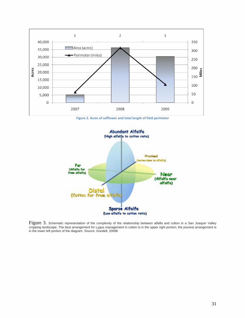
In the landscape, alfalfa acts as sponge, intercepting Lygus from other crops. When alfalfa habitat is managed, Lygus can be prevented from moving and establishing in cotton. By leaving a sufficient amount of uncut alfalfa during mowing in May and June, a large portion of the Lygus population can be herded into uncut strips (Summers et al 2004; Goodell, 2003). Similarly, if an area has an abundance and good distribution of alfalfa (Figure 3) in which cut and uncut fields are in close proximity, the uncut fields will act as a sink, drawing in Lygus from cut fields (Goodell, 2009b). In areas that have almost no alfalfa fields, Lygus is reported as a frequent problem in cotton. Having alfalfa in a landscape can provide a valuable management tool in mitigating Lygus movement into cotton and some farms have incorporated alfalfa as strategic part of their landscape plan. Implication of Deficit Irrigation in Alfalfa to Lygus IPM However, alfalfa can become as problematic as safflower if it is allowed to suffer irrigation stress. If the field is allowed to dry in July, Lygus will be forced out of the field just as if it were seed alfalfa. The alfalfa Lygus sink becomes a major Lygus source for cotton. The use of deficit irrigation on alfalfa as a water saving tactic has a major impact on IPM in the immediate area. Widespread adoption of deficit irrigation could shift the dynamics of the source/sink relations and result in increased risk to crop loss and increased use of insecticides to management Lygus. When deciding to place an alfalfa field into a deficit irrigation program, consider the field to be a source not a sink with resulting management risk and costs for bordering cotton. This role of alfalfa hay as major contributor to Lygus is a fundamental difference between southwestern desert landscapes and the SJV. In these areas, alfalfa hay is not harvested in mid-summer due to reduced quality and irrigation savings are implemented during this period. Management of the Lygus in the drying alfalfa field must be managed like safflower or alfalfa seed to prevent mass movement into susceptible cotton. Applications of insecticides will accomplish this goal but also destroy the natural enemy complex and disrupting an important ecological service alfalfa plays in the landscape. When developing landscape level IPM programs, it is essential that communication occur between production and pest management researchers. If a practice changes substantially the dynamics of the system, unintended consequences can occur. Integration between production and pest management is paramount if programs are to remain viable. Linking water issues with pest management is important. Communication is critical between industry working groups, UC work groups, as are discussions among participants at workshops, extension meetings, and state symposia. If deficit irrigation of alfalfa becomes more widespread, new approaches to Lygus management will be required. For example, an approach similar to strip harvest could be employed by continued irrigation on a limited, but critical number of strips in a field. These reduced acres could still be managed for harvest or simply watered to maintain them as suitable habitat to keep Lygus from moving. Each producer would need to conduct their own risk-benefit analysis to determine the value such an approach. The calculation of the degree of risk would still need to be conducted in order to truly determine the real cost of the decision. Component costs of allowing alfalfa to dry out in mid-summer might include:

29

• loss of production alfalfa hay (at expected quality for the period) • loss of cotton production due to increased Lygus damage • loss of ecological services provided by natural enemy complex in alfalfa • increased cost of insecticides to protect cotton • increased insecticide load in environment

Conclusion Changing major factors within landscape has substantial but unintended consequences. While the changes may be inevitable, the community within that ecological landscape can still develop approaches that mitigate predicted outcomes. This outcome is possible through communication and system integration to develop a new steady state in the landscape that minimizes risk to the environment, maximizes ecological services provided to the community and optimizes profit to the farmer. References: Adamczyk J.J. 2009. 62nd annual conference report on cotton insect research and control. Proceedings of the Beltwide Conferences, 2009:952-972 Carriere Y., Ellsworth P.C., Dutilleul P., Ellers-Kirk C, Barkley V. and Antilla L. 2006. A GIS-based approach for area-wide pest management: the scales of Lygus hesperus movements to cotton from alfalfa, weeds, and cotton. Ent Exp App 118(3):203–210 Goodell, P.B., 2003. Stripping (hay) for IPM: the value in maintaining Lygus habitat. Proceedings of the Alfalfa Seed Symposium, March 4, 2003. Five Points, CA. 10-12. Goodell, P.B. 2009a. Transcending spatial and temporal boundaries: What happens to IPM in cotton when landscapes radically change? Paper 35.3. 6th International IPM Symposium Program page 49. Goodell, PB. 2009b. Fifty years of the integrated control concept: the role of landscape ecology in IPM in San Joaquin Valley cotton. Pest Manag Sci 65:1293–1297 Goodell, P.B, K. Lynn and S.K. Mcfeeters. 2002. Using GIS approaches to study western tarnished plant bug in the SJV of California. Proceedings of the Beltwide Cotton Production Research Conferences. Atlanta GA. http://www.cotton.org/beltwide/proceedings/ Goodell, P.B., 2003. Stripping (hay) for IPM: the value in maintaining Lygus habitat. Proceedings of the Alfalfa Seed Symposium, March 4, 2003. Five Points, CA. 10-12. Goodell, P.B. and K. Lynn-Patterson. 2005. Managing Lygus in an ecological context. Proceedings of the Beltwide Cotton Production Research Conferences. New Orleans, LA. Proceedings of the Beltwide Conferences, 2005:1694-1701 Summers CG, PB Goodell, and Mueller SC. 2004. Lygus bug management by alfalfa harvest manipulation. Encyclopedia of Pest Management. (D Pimentel Editor) Vol. II. Pp. 322-325. CRC Press, Taylor & Francis Group, Boca Raton, FL.

30

Williams, M.R. 2009. Cotton insect losses. Proceedings Beltwide Cotton Conferences. San Antonio TX, 2009:897-940 Acknowledgements This work was made possible in part with a grant from USDA-CSREES Risk Avoidance & Mitigation Program (RAMP). The contribution of Doug Cary, Nathan Cannell, Idalia Orellana, Ashley Pedro and the GIS Laboratory at Kearney Ag Center is greatly appreciated. The cooperation of PCAs and farmers on the Westside of Fresno and Kings Counties is deeply appreciated and would not be possible without their support. Figures

Figure 1. Safflower acreage in Fresno‐Kings Counties from 2007 to 2009. Area was mapped as part of USDA‐CSREES RAMP study. Note the concentration of acres and minimizing of contact between safflower and bordering crops during the three year time period.

31

Figure 2. Acres of safflower and total length of field perimeter

Figure 3. Schematic representation of the complexity of the relationship between alfalfa and cotton in a San Joaquin Valley cropping landscape. The best arrangement for Lygus management in cotton is in the upper right portion; the poorest arrangement is in the lower left portion of the diagram. Source: Goodell, 2009b

32

Movement of Glassy-Winged Sharpshooter in a Deficit-Irrigated Citrus Orchard Rodrigo Krugner, USDA-ARS, San Joaquin Valley Agricultural Sciences Center, Parlier, CA

Russell L. Groves, Department of Entomology, University of Wisconsin, Madison, WI

Marshall W. Johnson, Department of Entomology, University of California, Riverside, CA James R. Hagler, USDA-ARS, Arid-land Agricultural Research Center, Maricopa, AZ Joseph G. Morse, Department of Entomology, University of California, Riverside, CA

Abstract. A two-year study was conducted in a citrus orchard [Citrus sinensis (L.) Osbeck cv. ‘Valencia’] to determine the effects of plant water stress on population density and movement of glassy-winged sharpshooter (GWSS), Homalodisca vitripennis (Germar). Experimental treatments included irrigation at 100% of the crop evapotranspiration rate (ETc) and continuous deficit-irrigation regimes at 80 and 60% ETc. Microclimate and plant conditions monitored included temperature and humidity in the tree canopy, leaf surface temperature, water potential, and fruit quality and yield. GWSS population density was monitored weekly by a combination of visual inspection, beat net sampling, and trapping. Movement of GWSS among treatment plots was quantified through a mark and capture technique using protein markers (soy milk, whole milk, and egg white) and yellow sticky traps. GWSS populations were negatively affected by severe plant water stress; however, population density was not linearly related to decreasing water availability in plants. Citrus trees irrigated at 60% ETc had significantly warmer leaves, lower xylem water potential, and consequently hosted fewer GWSS eggs, nymphs, and adults than trees irrigated at 80% ETc. Citrus trees irrigated at 100% ETc hosted similar numbers of GWSS as trees irrigated at 60 and 80% ETc. Although the adult GWSS population was reduced, on average, by 50% in trees under severe water stress, the total number of fruit and number of fruit across several fruit grade categories were significantly lower in the 60% ETc than in the 80 and 100% ETc irrigation treatments. The spatiotemporal distribution and movement of GWSS in the orchard will be discussed with emphasis on the development of strategies to focus control efforts, enhance the efficacy of biological control, and effectively limit the spread of Xylella fastidiosa induced diseases to susceptible crops. Introduction The glassy-winged sharpshooter (GWSS), Homalodisca vitripennis (Germar), is a xylem fluid-feeding leafhopper that transmits the bacterium Xylella fastidiosa Wells et al. into peach (Turner 1959), almond (Almeida and Purcell 2003), citrus (Damsteegt et al. 2006), and grapevines (Purcell and Saunders 1999) where it causes Pierce’s Disease (PD) (Davis et al. 1978). It is a highly polyphagous leafhopper with over 100 known hosts (Turner and Pollard 1959), but citrus is the most common overwintering and first generation reproductive host found in southern California (Blua et al. 1999). Therefore, with over 109,384 ha of citrus distributed throughout the state and nearly 13.1% of these hectares (14,356 ha) treated with imidacloprid in 2006 alone (CDFA 2006), integrated management tactics that are considered more ecologically sustainable and have less overall reliance on area-wide insecticide applications are warranted. During the last 40 years, a considerable volume of information has been generated to characterize the impact of plant water stress on insect outbreaks and regulation of insect

33

population dynamics. In general, resulting responses often appear to be insect feeding-guild dependent. In a recent analysis, which included results from 116 published studies, Huberty and Denno (2004) found strong negative effects of water stress on phloem-, xylem-, and mesophyll-feeders. Among the selected studies, only one study investigated the effect of plant water stress on the performance of a xylem feeder. While the effect of plant water stress appears to be deleterious to xylem feeding sharpshooters, deficit irrigation regimes applied during less vulnerable phenological stages of citrus fruit development have caused little to no impact, and in some instances, increased gross yields, fruit loads, and fruit quality (Goldhamer and Salinas 2000). Although significant new information is becoming available regarding the host selection behavior of xylem feeding insects, little is understood regarding the effect of plant water stress on GWSS population dynamics, which is critical to improving our understanding of vector ecology. The goal of this research was to generate novel information useful in the development of sustainable management strategies for control of GWSS populations, which might limit the spread of X. fastidiosa into susceptible crops. The objectives were to investigate the effects of continuous deficit irrigation regimes in citrus trees on the population dynamics of GWSS and associated natural enemies. Materials and Methods The study was conducted at Agricultural Operations at the University of California, Riverside, from April 2005 to June 2007 in a citrus orchard (cv. ‘Valencia’) that received three irrigation treatments: 1) trees irrigated at 100% of the crop evapotranspiration (ETc), 2) a continuous deficit-irrigated treatment maintained at 80% ETc, and 3) a continuous deficit-irrigated treatment at 60% of ETc. Plant conditions monitored included temperature and humidity in the tree canopy, leaf surface temperatures, and pre-dawn trunk water potential. In June 2006 and 2007, all oranges were harvested and immediately taken to a local commercial packing house where oranges were mechanically counted, sized, and color graded. Measurements of fruit sugar solids (°Brix) were also recorded. Populations of GWSS were sampled weekly from April 2005 to Dec 2005 and Feb 2006 to Dec 2006. A 3-min visual inspection of leaves and branches around sample trees was conducted to monitor for GWSS egg masses, nymphs, adults, and natural enemies. GWSS population density was also monitored by collecting beat net samples. Yellow sticky traps and protein markers were used to monitor insect activity and movement among irrigation treatments. Results Effect of irrigation deficit on microclimate and plant conditions. Higher temperatures inside the tree canopy were recorded during May to Sept 2005 in the 60% ETc treatment than in the 100% ETc treatment. Throughout the study, there were no significant differences in canopy relative humidity among the treatments. In general, leaf surface temperatures of trees irrigated with 60% ETc were higher than those of trees irrigated with 80% and 100% ETc. There was no difference between the 80% and 100% ETc treatments. Pre-dawn water potential measurements were lower in the 60% ETc treatment than in the 80% or 100% ETc treatments recorded among all time periods. There were no differences in water potential between the 80% and 100% ETc

34

treatments. In 2006, no differences in fruit sugar solid content were detected among the irrigation treatments. In 2007, fruit sugar solid contents were higher in trees irrigated at 60% (14.22 ± 0.19 °Brix) and 80% ETc (14.31 ± 0.17) than at 100% ETc (13.56 ± 0.15). In 2006, there were no differences in total numbers of harvested fruit and number of fruit per grade category among irrigation treatments. In 2007, the total number of harvested fruit and numbers of fruit across all fruit grade categories in the 60% ETc treatment were significantly lower than in the 80% and 100% ETc treatments. There were no significant differences in total number of fruit and number of fruit per grade category between the 80% and 100% ETc irrigation treatments. Effect of irrigation deficit on GWSS populations. During the visual inspections in 2005, fewer GWSS adults were found on trees irrigated with 60% of the ETc than with 80% and 100% ETc. There was no difference in the number of GWSS adults found per tree between the 80% and 100% ETc treatments. On average (± SEM), 1.1 ± 0.4, 2.4 ± 1.0, and 1.9 ± 0.4 GWSS adults were found per tree at the population peak in mid-July 2005 in the 60%, 80%, and 100% ETc treatments, respectively. In 2006, up to the peak of GWSS numbers in late-July, fewer adults were found on trees irrigated at 60% of the ETc than at 80% and 100% ETc. There was no difference in the number of GWSS adults found per tree between 80% and 100% ETc treatments. In the early-July to early-Oct interval, fewer adult GWSS were found in trees irrigated at 60% of the ETc than at 80% ETc. The number of adult GWSS was not different in the 100% ETc treatment vs. those in the 60% or the 80% ETc treatments. On average (± SEM), 5.4 ± 0.7, 13.1 ± 2.8, and 10.8 ± 1.7 adult GWSS were observed in visual counts per tree at the peak period in late-July 2006 in the 60%, 80%, and 100% ETc treatments, respectively. In 2005 and 2006, less than 1.0 and 2.2 GWSS egg masses were found per sampled tree per week, respectively. In 2005, no differences in the mean number of GWSS egg masses were observed among the irrigation treatments. In 2006, there appeared to be four peaks of GWSS oviposition. The first peak occurred between late-Feb to early-March. A second peak occurred from late-April to early-June and the third peak occurred between early-July to early-Sept. A discrete fourth peak occurred between late-Sept to late-Oct. Fewer GWSS egg masses were found in the 60% ETc treatment in comparison to the 80% or 100% ETc treatments during the second peak oviposition period of 2006. Yellow sticky traps documented the presence of adult GWSS throughout the 117 weekly trapping periods, but trapping periods after early-June showed a steady increase in insect activity to a peak in late July 2005 and 2006, with an average (± SEM) of 11.96 ± 1.16 and 95.22 ± 4.81 adults caught per trap per week, respectively. There were no differences in numbers of GWSS adults per trap per week among the irrigation treatments. Discussion Our measurements of microclimate and plant conditions in this field experiment indicated that water stress increased leaf surface temperatures and decreased trunk water potential. The two irrigation deficit regimes, 60% and 80% ETc, differentially affected the population dynamics of GWSS in the experimental citrus plots. Severe to moderate water-stressed trees (60% and 80% ETc) perhaps had increased solute concentrations used for osmotic adjustment (i.e., carbohydrates, amino acids, and organic acids) that might serve as feeding stimulants and

35

primary nutrients of insects (Mattson and Haack 1987). However, decreased water potential in more severe water-stress irrigation treatments (60% ETc) might have been an impediment to GWSS feeding because more energy would be required to extract xylem fluid out of the xylem vessels (Andersen et al. 1992). In contrast, well-watered plants (100% ETc) had lower mean water potentials that potentially facilitated extraction of xylem fluid, but more fluid would have to be ingested and filtered to compensate for a more dilute xylem food source. Thus, citrus trees irrigated with 80% ETc may combine two important plant characteristics for GWSS: 1) a nutrient-concentrated food source and 2) a water potential at acceptable levels for GWSS xylem fluid extraction, at least during periods of low transpirative demand by plants. Conclusion Findings from this study have generated significant new information regarding the host selection behavior of GWSS in California. Trees under severe water stress hosted fewer GWSS than trees maintained under moderate water stress. A more complete understanding of the effect of shorter water stress periods (i.e., regulated deficit irrigation regimes) and the operative host-plant cues that influence GWSS host selection behavior may result in the deployment of strategies to improve control efforts and contribute to limiting the spread of Xf induced diseases to susceptible crops. Funding Agencies Funding for this project was provided by the UC Division of Agriculture and Natural Resources, PD and GWSS Research Grants Program, the USDA-ARS, and a Specific Cooperative Agreement between the USDA-ARS and UC Riverside. References

Almeida, R.P.P., and A.H. Purcell. 2003. Homalodisca coagulata (Hemiptera: Cicadellidae)

transmission of Xylella fastidiosa to almond. Plant Dis. 87: 1255-1259. Andersen, P.C., B.V. Brodbeck, and R.F. Mizell III. 1992. Feeding by the leafhopper,

Homalodisca coagulata, in relation to xylem fluid chemistry and tension. J. Insect Physiol. 38: 611-622.

Blua, M.J., P.A. Phillips, and R.A. Redak. 1999. A new sharpshooter threatens both crops and ornamentals. Calif. Agric. 53: 22-25.

CDFA. 2006. County agricultural commissioner’s data, calendar year 2005. California Department of Food and Agriculture, Sacramento, CA, USA.

Damsteegt, V.D., R.H. Brlansky, P.A. Phillips, and A. Roy. 2006. Transmission of Xylella fastidiosa, causal agent of citrus variegated chlorosis, by the glassy-winged sharpshooter, Homalodisca coagulata. Plant Dis. 90: 567-570.

Davis, M.J., A.H. Purcell, and S.V. Thompson. 1978. Pierce’s disease of grapevines: isolation of the causal bacterium. Science 199: 75-77.

Goldhamer, D.A. and M. Salinas. 2000. Evaluation of regulated deficit irrigation on mature orange trees grown under high evaporative demand, pp. 227-231. In Proc., Intl. Soc. Citricult. IX Congr. ASHS Press, Alexandria, VA, USA.

36

Huberty, A. and R. Denno. 2004. Plant water stress and its consequences for herbivorous insects: a new synthesis. Ecology 85: 1383-1398.

Mattson, W.J., and R.A. Haack. 1987. The role of drought stress in provoking outbreaks of phytophagous insects, p. 365-408. In P. Barbosa and J. C. Schultz (eds.), Insect Outbreaks. Academic Press, Inc.: San Diego, California, USA; London, England, UK.

Purcell, A.H., and S.R. Saunders. 1999. Glassy-winged sharpshooter expected to increase plant disease. Calif. Agric. 53: 26-27.

Turner, W.F. 1959. Insect vectors of phony peach disease. Science 109: 87-88. Turner, W.F., and H.N. Pollard. 1959. Life histories and behavior of five insect vectors of

phony peach disease. U. S. Dep. Agric. Tech. Bull. 1188: 1-28.

37

Session II

Nutrient Management

Session Chairs:

Sharon Benes, CSU, Fresno Nathan Heeringa, Innovative Ag Services

38

Developing testing protocols to ensure the authenticity of fertilizers for organic agriculture

William R. Horwath, Professor of Soil Biogeochemistry

3226 Plant and Environmental Science Building, One Shields Ave., University of California, Davis, CA 95616, Tel: 530-754-6029, wrhorwath@ucdavis.edu

Introduction

There is growing concern about the authenticity and integrity of soil and crop amendments sold for use in organic production (“Organic farms unknowingly use synthetic fertilizer”, Sacramento Bee, Dec 28, 2008; see also letter from the Executive Director of the Organic Materials Review Institute, Feb. 20, 2009, http://omri.org/OMRI_PR.html). For example, synthetic ammonia is not permitted in organic production, but it may be added to a product claimed to be derived from fish because, as expected, the resulting product is very effective as a fertilizer, much cheaper to produce, and ensures a higher profit for the manufacturer. In addition, the product quality and consistency is enhanced giving the illusion that the “organic fertilizer” is of a better grade than other materials, or competing products on the market. Since much of the organic amendment certification process is based on trust, such adulterated products are often approved and labeled as suitable for organic agriculture. Depending on the degree of adulteration, basic laboratory tests often cannot indicate a problem. Analysis of nitrogen content, for example, may confirm a product label, but will not indicate the source of nitrogen. The problem has undermined public trust in the “organic” label of produce in California, and this could negatively affect growers of organic foods.

The development of guidelines and protocols to test organic fertilizers for their authenticity will contribute to restoring trust in producers of organic fertilizers, fairness of the marketplace, and the confidence of consumers being offered produce that has been grown according to organic standards. These guidelines and protocols are directly related to the goals of assisting the organic fertilizer industry efforts to increase public confidence in the food supply and to provide for an equitable marketplace.

There is a need to provide methods so that testing labs and regulatory agencies can detect adulteration of organic fertilizers. The development of such methods will provide the basis to develop standards to ensure the authenticity of organic amendments. The success of the guidelines and protocols will ensure that manufacturers of adulterated organic fertilizers and amendments will face the appropriate scrutiny to ensure the authenticity of their products. Legitimate producers of fertilizers will benefit by having a defined set of testing protocols to ensure the quality of their products. The guidelines and protocols will contribute to greater transparency and authenticity of fertilizer products intended for organic agriculture.

The need for research Previously, no systematic research has been undertaken to develop comprehensive

guidelines on testing the authenticity of organic fertilizers and amendments. However, some of the techniques that can be incorporated into the testing protocols, such as the use of stable isotope analysis, have been used in criminal forensic, ecosystem and physiological studies. Important to developing guidelines and protocols is the biogeochemical literature that addresses the sources, fractionation and pathways of carbon, nitrogen and oxygen isotopes within different

39

trophic levels of food webs and unique organismal metabolic pathways (Schimel 1993; Horwath et al. 2001). Other methodologies such as Fourier Transform Infrared (FTIR) and thermogravimetric techniques have been used extensively for forage quality analysis and in the food industry (van Groenigen and Horwath et al., 2001). A great deal of information that can be used to develop guidelines and protocols can be found in the literature although this information is highly fragmented (Table 1). Table 1. Examples of measured properties of materials potentially used in organic fertilizers and as adulterants, as reported in the scientific literature. The properties are the isotope ratios of carbon and nitrogen (d13C and d15N), carbon content (%C), nitrogen content (%), carbon to nitrogen ratio (C:N), and phosphorus content (%P).

delta 13C delta 15N %C %N C:N ratio

%P Reference

Commercial products

fish meal (anchovy)

-18 -13 42 11 to 3.8 Yokoyama et al. 2006

fish meal (herring)

11.5 1.7 Luzier et al. 1995

Natural materials

fish protein -22 to -17 10 to 16 3 to 5 Sherwood and Rose 2005

seabird guano

-20 to -18 9 to 11 22 13 to 17

Mizutani and Wada 1988

Synthetic materials

fertilizer ammonium

-4 to 2 Freyer and Aly 1974

urea -41 -1 Vitoria et al. 2004

The following example illustrates how a relatively simple measurement such as the carbon to nitrogen (C:N) ratio with a suggested threshold value, may be used to question the integrity of an organic fertilizer product (Figure 1). The preliminary data shown in Figure 3 represent fish-based fertilizers from several different suppliers. The N contained in fish tissue is organic, consisting primarily of protein-derived amino acids, which range in C:N from just above 1 to approximately 8. A product derived exclusively from fish should therefore not have a C:N lower than about 1 or 2, even in the extreme case that the protein consisted of mostly N-rich amino acids, such as arginine. Adulteration with ammonia/ammonium would increase the amount of N relative to C, decreasing the C:N ratio such that a C:N ratio that is too low could indicate some degree of adulteration. Indeed, all of the products which show a low C:N have the potential of

40

being adulterated. In combination with a more advanced measurement such as nitrogen isotope ratio (expressed as δ15N), a stronger tentative assessment can be done. Synthetic nitrogen has a low (zero to negative) δ15N value relative to fish-nitrogen (see table 1). This is because synthetic N is derived from atmospheric N2 (with a δ15N of zero), whereas animal tissues have higher δ15N values reflecting biochemical preference for retaining the heavier isotope as new tissue is synthesized and as the food chain advances to higher trophic levels (Peterson and Fry 1987, Kendall 1998). The addition of synthetic N to a product would therefore tend to lower the δ15N of an organic fertilizer derived solely from fish. Figure 1 shows that the samples with a low C:N ratio also had a relatively low δ15N value. As expected, there was a relationship between C:N and δ15N.

0

2

4

6

8

10

12

14

16

0 1 2 3 4 5 6C:N

d15N

Figure 1. The carbon to nitrogen ratio vs. the δ15N value of 11 fish-based fertilizers analyzed in our lab and at the UC Davis Stable Isotope Facility.

Other properties, such as ash content, nitrogen to phosphorus ratio, phosphorus content, and content of other elements, can vary widely depending on the nature of a product and the way in which it has been processed. For example, a product made primarily from fish flesh scraps (no bones) has less ash, phosphorus, and calcium compared to a product made from whole fish or fish offal. Nevertheless, such parameters may still be used to evaluate a product if the manufacturer’s claims regarding its composition are considered.

Constructing guidelines for quality assurance The evaluation and principal trends of properties of materials used to make organic fertilizers can be incorporated into a recommended course of action as shown in Figure 2. The flowchart is based on findings, such as those listed in Table 1. According to our present knowledge, the C:N ratio would be an easy-to-measure property giving a strong indication on the authenticity of a tested product. If the C:N ratio was suspect, further tests could be

Figure 2. A conceptual flow chart showing a recommended course of action for test labs and regulatory agencies. The purpose of these actions is to ascertain the authenticity of organic fertilizers. The example is based on preliminary results and illustrates how a series of tests will lead to a recommended inspection of a manufacturing facility if results look suspect.

41

recommended. Measurement of isotope ratios of C, N, and O would be recommended if multiple variables suggested that adulteration of a natural product with synthetic fertilizer might have occurred.

The guidelines for the testing labs and regulatory agencies will include all the information about a material and possible steps that need to be taken to evaluate such a product. The guidelines will provide the organic industry the tools necessary to evaluate fertilizers and ensure that the trust in the organic label has integrity.

References Freyer HD, Aly AIM. 1974. Nitrogen-15 variations in fertilizer nitrogen. Journal of Environmental Quality 3:405-406.

Horwath, W.R., C. van Kessel, U. Hartwig and D. Harris. 2001. Use of 13C isotopes to determine net carbon sequestration in soil under ambient and elevated CO2. R. Lal, J.M. Kimble, R.F. Follett and B.A. Stewart, Eds. Chapter 16 In: Assessment Methods for Soil Carbon. pp. 221-232.

Kendall C. 1998. Tracing nitrogen sources and cycles in catchments. In: Isotope Tracers in Catchment Hydrology. Kendall C, McDonnell JJ (Eds.) Elsevier.

Luzier JM, Summerfelt RC, Ketola HG. 1995. Partial replacement of fish meal with spray-dried blood powder to reduce phosphorus concentrations in diets for juvenile rainbow trout. Aquaculture Research 26:577-587.

Mizutani H, Wada E. 1988. Nitrogen and carbon isotope ratios in seabird rookeries and their ecological implications. Ecology 69:340-349.

Peterson BJ, Fry B. 1987. Stable isotopes in ecosystem studies. Annual Review of Ecology and Systematics 18:293-320.

Schimel, DS, 1993. Theory and application of tracers. Academic Press, Inc., San Diego California.

Sherwood GD, Rose GA. 2005. Stable isotope analysis of some representative fish and invertebrates of the Newfoundland and Labrador continental shelf food web. Estuarine, Coastal and Shelf Science 63:537-549.

van Groenigen, J.W., C.S. Mutters, W.R.Horwath, and C. van Kessel. 2003. NIR and DRAFT-MIR spectrometry of soils for predicting soil and crop parameters in a flooded field. Plant and Soil 250:155-165.

Vitoria L, Otero N, Soler A, Canals A. 2004. Fertilizer characterization: isotopic data (N, S, O, C, and Sr). Environmental Science and Technology 38:3254-3262.

Yokoyama H, Abo K, Ishihi Y. 2006. Quantifying aquaculture-derived organic matter in the sediment in and around a coastal fish farm using stable carbon and nitrogen isotope ratios. Aquaculture 254:411-425.

42

43

44

45

46

47

48

Nutritional Considerations When Converting to Micro-Irrigation

Jerome Pier, Ph.D., North Valley Division Agronomist, Crop Production Services, 509 West Weber Ave., Suite 201, Stockton, CA 95203

Phone (209) 610-0565, FAX (209) 464-4652, jerome.pier@cpsagu.com Introduction

Several factors are causing California growers to convert to micro-irrigation. Limited water availability, higher yields, environmental pressures and erratic fertilizer pricing are just a few of the reasons growers are deciding that drip or micro-sprinkler irrigation is a practical option. There are many highly qualified irrigation dealers available to design and install efficient, high performance micro-irrigation systems. However, there is a lack of after-sales agronomic support for first time micro-irrigation users. There are major agronomic differences between managing a flood, furrow, or sprinkler irrigation system and a micro-irrigation system. This presentation will give a new micro-irrigation user some plant nutrition guidelines to help shorten the learning curve.

Irrigation System Comparison Flood or furrow irrigation applies large volumes of water by gravity over long time periods. Flood irrigation intervals are long and application uniformities can be 50% or less. Solid set or impact sprinkler irrigation applies smaller volumes of water than flood irrigation fairly uniformly over large areas and water is applied more frequently. Sprinkler application uniformities are normally better than flood systems but there are potential water losses due to evaporation and wind may affect application uniformity. Micro-sprinklers apply smaller volumes of water over smaller areas than solid set sprinklers and have improved applications uniformities. Finally, surface and sub-surface drip irrigation apply the smallest amounts of water frequently and have the highest application uniformity of any irrigation system (Table 1.) Reduced water applications through micro-irrigation are due to the reduction in water being lost to leaching below the root zone, run-off and evaporation. The crop demands for water to achieve maximum yields do not change between systems, just the efficiency of water delivery changes.

Table 1 Ranges of application efficiencies for several irrigation systems. 1

Irrigation System Application Efficiency % Applied water to provide 1 inch in root zone

Furrow 35-60 1.7 - 2.8 Solid Set Sprinkler 60-85 1.2 – 1.7 Micro-spray 85-90 1.1 – 1.2 Surface or sub-surface drip 90-95 1.05 – 1.1

1Adapted from Sterling and Neibling. 1994. Final Report of the Water Conservation Task Force. IDWR Report. Idaho Department of Water Resources, Boise

Fertilizer Choices for Micro-Irrigation Micro-irrigation applies low volumes of water under low operating pressures. This is possible due to plastic emitters that create turbulent flow that dissipates the energy of water under pressure. The cross-sectional diameters of micro-irrigation emitters are very small. This means that micro-irrigation systems are susceptible to plugging from particulate matter. All

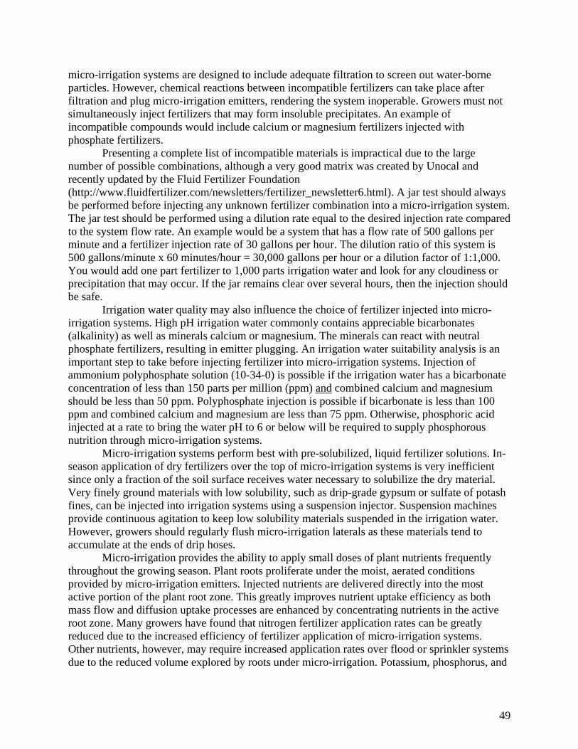
49

micro-irrigation systems are designed to include adequate filtration to screen out water-borne particles. However, chemical reactions between incompatible fertilizers can take place after filtration and plug micro-irrigation emitters, rendering the system inoperable. Growers must not simultaneously inject fertilizers that may form insoluble precipitates. An example of incompatible compounds would include calcium or magnesium fertilizers injected with phosphate fertilizers.

Presenting a complete list of incompatible materials is impractical due to the large number of possible combinations, although a very good matrix was created by Unocal and recently updated by the Fluid Fertilizer Foundation (http://www.fluidfertilizer.com/newsletters/fertilizer_newsletter6.html). A jar test should always be performed before injecting any unknown fertilizer combination into a micro-irrigation system. The jar test should be performed using a dilution rate equal to the desired injection rate compared to the system flow rate. An example would be a system that has a flow rate of 500 gallons per minute and a fertilizer injection rate of 30 gallons per hour. The dilution ratio of this system is 500 gallons/minute x 60 minutes/hour = 30,000 gallons per hour or a dilution factor of 1:1,000. You would add one part fertilizer to 1,000 parts irrigation water and look for any cloudiness or precipitation that may occur. If the jar remains clear over several hours, then the injection should be safe.

Irrigation water quality may also influence the choice of fertilizer injected into micro-irrigation systems. High pH irrigation water commonly contains appreciable bicarbonates (alkalinity) as well as minerals calcium or magnesium. The minerals can react with neutral phosphate fertilizers, resulting in emitter plugging. An irrigation water suitability analysis is an important step to take before injecting fertilizer into micro-irrigation systems. Injection of ammonium polyphosphate solution (10-34-0) is possible if the irrigation water has a bicarbonate concentration of less than 150 parts per million (ppm) and combined calcium and magnesium should be less than 50 ppm. Polyphosphate injection is possible if bicarbonate is less than 100 ppm and combined calcium and magnesium are less than 75 ppm. Otherwise, phosphoric acid injected at a rate to bring the water pH to 6 or below will be required to supply phosphorous nutrition through micro-irrigation systems.

Micro-irrigation systems perform best with pre-solubilized, liquid fertilizer solutions. In-season application of dry fertilizers over the top of micro-irrigation systems is very inefficient since only a fraction of the soil surface receives water necessary to solubilize the dry material. Very finely ground materials with low solubility, such as drip-grade gypsum or sulfate of potash fines, can be injected into irrigation systems using a suspension injector. Suspension machines provide continuous agitation to keep low solubility materials suspended in the irrigation water. However, growers should regularly flush micro-irrigation laterals as these materials tend to accumulate at the ends of drip hoses.

Micro-irrigation provides the ability to apply small doses of plant nutrients frequently throughout the growing season. Plant roots proliferate under the moist, aerated conditions provided by micro-irrigation emitters. Injected nutrients are delivered directly into the most active portion of the plant root zone. This greatly improves nutrient uptake efficiency as both mass flow and diffusion uptake processes are enhanced by concentrating nutrients in the active root zone. Many growers have found that nitrogen fertilizer application rates can be greatly reduced due to the increased efficiency of fertilizer application of micro-irrigation systems. Other nutrients, however, may require increased application rates over flood or sprinkler systems due to the reduced volume explored by roots under micro-irrigation. Potassium, phosphorus, and

50

micronutrients that are taken up by diffusion may become rapidly depleted under micro-irrigation. Providing ideal soil moisture and plant nutrition may also result in an increased yield potential such that, even though there is an improvement in nutrient uptake efficiency, there may be an overall increased fertilizer requirement. Plant tissue testing is a valuable tool to help inexperienced growers adjust fertilizer application rates to micro-irrigation.

Timing of fertigation during the irrigation set is an important factor in deriving the benefits of micro-irrigation. All pressurized irrigation systems require a certain amount of time to fill all laterals with water and achieve operating pressure. Injected fertilizers also require a certain amount of time to distribute throughout the micro-irrigation system. More-importantly, it takes longer to flush fertilizers from the slow moving water in micro-irrigation laterals than it does to distribute them. Therefore, the ideal time to inject fertilizer takes place in the middle of the irrigation set. If injection takes place before achieving operating pressure, there is a loss in fertilizer distribution uniformity. If the irrigation system is shut down soon after the end of the fertilizer injection, fertilizer remains in the laterals, encouraging microbial growth that can lead to plugging. A general rule of thumb is to stop fertilizer injection for an amount of time equal to twice the amount of time it takes to bring the system to operating pressure.

The timing of injection becomes more important when applying long set times to perennial crops requiring deep soil moisture. During long irrigations, mobile nutrients such as nitrate-nitrogen, urea-nitrogen, chelated micronutrients and others, can be leached below the root zone. Therefore, nutrients mobile in soil should be applied near the end of a long irrigation set while still allowing time for adequate flushing.

Water availability and economic pressures are increasing the number of growers converting to micro-irrigation. A knowledge of water quality and fertilizer compatibilities and micro-irrigation characteristics will allow new users to enjoy all the benefits of micro-irrigation without suffering from it’s limitations.

51

Fertilizer Prices: Getting the Right Information to Make Good Decisions

Robert Mikkelsen, International Plant Nutrition Institute 4125 Sattui Ct. Merced, CA 95348

Phone (209) 725-0382 (rmikkelsen@ipni.net) Introduction Rapid increases in fertilizer prices made headline news in 2008, causing politicians and the general public to be more aware of the fertilizer industry than ever before. As the prices of wheat, rice, and corn more than doubled, food riots erupted in some countries and caused governments to impose limits on crop exports. While the urgency associated with the food crises no longer appears in the headlines, the number of undernourished people in the world continues to grow. Fertilizer nutrients are worldwide commodities that are associated with global economics and demand, as well as societal stability. It is estimated that commercial fertilizer is responsible for 40 to 60% of the world’s food production (Stewart et al, 2005). World fertilizer consumption increased steadily from the early 1960’s through the mid 1980’s and declined through the mid 1990’s before rising again. It is clear that commercial fertilizer is necessary to maintain global food production at current levels and will become increasingly important as harvests must increase to match population growth. Proper management of nutrient sources is essential for meeting the challenges of increasing food production and achieving environmental goals. Making Fertilizer Decisions: Right Source, Right Rate, Right Time, Right Place (4Rs) Many factors are considered when making decisions related to nutrients. Although price is an important consideration, there are many other significant factors that must also be accounted for in arriving at a final purchase decision. Some of these factors can be easily quantified, but increasingly they include environmental, social, or economic factors. The decisions relate to selecting the nutrient that will provide the right source, which can be supplied to the crop at the right rate, applied at the right time, and delivered at the right place. While fertilizer price factors into these decisions, economic factors alone are not the only issue. I recently purchased a new car. In the process of making a selection, I knew that I could choose from many vehicles that could provide satisfactory transportation and get me to my destination. I then began to consider factors such as safety, reliability, fuel economy, comfort, and size. Many options were available to me as long as I was willing to pay for them. The price of a car from the dealer all depended on what features I wanted and could negotiate from competing dealers. Fertilizer pricing is also based on similar market principles. Where there is more than one fertilizer supplier in a region, a buyer generally looks for the best deal to meet the overall production goals. This will certainly include the fertilizer price, but also includes considerations of transportation, timeliness, financing, crop advice, and the availability of other production inputs. The lowest price is not always the best value.

52

A Closer Look at Key Nutrients: Nitrogen: At one time, North America was relatively self sufficient in nitrogen production. However, the U.S. is now the largest importer of nitrogen in the world. Natural gas is the primary raw material used in the synthesis of anhydrous ammonia, which is the fundamental product for making all N fertilizers. Natural gas accounts for 75 to 90% of the cost of ammonia production. Generally, the price of natural gas determines whether a nitrogen fertilizer plant will operate or not. Consider that industrial natural gas prices increased from $3/thousand cubic feet in 1998 to approximately $10 in 2008, and are currently near $6. North America producers use some of the most expensive natural gas in the world. For example, in 2006, the U.S. dollar price for natural gas (mm BTU) was $6.75 in the U.S., Latin America gas was between $0.85 to $2.50, Russian gas was $1.25, and North Africa/Middle Eastern natural gas was $0.75. Since natural gas is such an important cost in manufacturing nitrogen fertilizer, it is easy to see why production has shifted overseas to areas where energy is less expensive. Most of the imported ammonia is priced by obtaining quotes for delivery at New Orleans, Louisiana (NOLA), the main entry point for North America. Costs of freight, dollar exchange rates, broker profit, and warehousing add to the price. At the retail location, the local dealer needs to add their costs, blending expenses, risk, and a return on their investment to make delivery profitable. All of the fertilizer nitrogen in California is imported, largely by ocean vessel and rail car, thus transportation costs play a significant role in the final fertilizer price. Phosphorus: The main raw material used in the production of nearly all phosphate fertilizers is phosphate rock. Figure 1 shows the global deposits of rock phosphate currently being mined, those that have been mined in the recent past, and those shown to be potentially economic (McClellan and Van Kauwenbergh, 2004). The closest commercial rock phosphate deposits for California are the reserves in the south-east corner of Idaho, western Wyoming, and northern Utah. Additional expenses associated with environmental regulations and increasing difficulty in obtaining phosphate ore mining permits are hampering expansion in many areas of the U.S. Shifts in prices for natural gas and sulfur are manifested in increased phosphate fertilizer prices, since these components are required in processing rock phosphate and producing ammoniated phosphorus fertilizers. Sulfur is oxidized to sulfuric acid and reacted with the mined rock to solubilize the phosphate from the raw minerals. Ammonia is reacted with phosphoric acid to produce common phosphate fertilizer sources such as such as monoammonium phosphate, diammonium phosphate, and polyphosphate. Sulfur: Sulfur is one of the more common elements of the Earth’s crust. Most of the sulfur used in agriculture is extracted from natural gas and crude oil, since these fossil fuels contain between 0.1 to 3% S. Most of the world’s sulfur production is used to manufacture sulfuric acid and half of that is used for fertilizer production (mostly for processing rock phosphate). About one ton of sulfur is needed to produce a little more than 2 tons of diammonium phosphate.

53

Potassium: Potassium fertilizer (potash) comes from a variety of minerals, the most common being sylvite (KCl), sylvinite (KCl+NaCl) and langbeinite (K2SO4+MgSO4). The largest potassium reserves are located in Canada, while Russia, Belarus, and Germany also have large reserves. New production is expected in several locations of the world. The current cost of opening a new mine, such as those currently operating in central Canada is several billion dollars, posing a significant financial risk for new entry into the market when prices for the final product can change rapidly. The largest potassium production area in the U.S. is near Carlsbad, New Mexico. Utah is also the location of limited potassium production from the Great Salt Lake area and underground deposits near Moab. California once had a thriving potassium mining industry near the town of Trona, which is located in the region of Death Valley, CA. Fertilizer Pricing Issues: Fertilizer is a global commodity that is traded widely across the globe. Since it is a mature and valuable industry, there is a sophisticated infrastructure in place to allow this international trade to occur quickly and efficiently. There are several excellent industry publications that provide an overview of wholesale fertilizer prices on a regular basis. The most widely cited source of domestic fertilizer industry news and prices is the weekly publication “Green Markets”, an electronic newsletter available by subscription. Green Markets provides average wholesale fertilizer prices for many materials in key parts of North America, including California. Other commercial publications (such as Fertecon and ICIS Pricing) are also available by subscription. Global prices of a few key fertilizers are provided free by <www.fertilizer-index.com/Price-Index.asp> . The British publisher BCInsight Ltd. publishes several excellent magazines that cover global fertilizer issues (such as Fertilizer International; Nitrogen and Syngas; Sulphur). Similarly, FMB Consultants publishes a comprehensive magazine, Fertilizer Focus. A useful compilation of historic retail fertilizer prices is maintained by the USDA Economic Research Service. Although their statistical analysis lags behind by one year, it provides a reliable view of fertilizer markets in the United States. <www.ers.usda.gov/Data/FertilizerUse> Commercial fertilizer dealers in California are in daily contact with their wholesale suppliers to provide up-to-date information on pricing status that can change rapidly in response to global events. The local retail prices reflect added expenses due to transportation, regulatory requirements, labor, storage, blending, handling, and farm delivery. This additional cost will vary from region to region within the state and can change with the season of the year. For current retail pricing information, it is necessary to directly contact a local dealer to get an accurate quote.

54

Organic Sources of Nutrients: The market for organic nutrient sources is not sufficiently developed to have a centralized point of price information. The value of the essential plant nutrient may to some degree follow trends associated with the price of commercial fertilizer and its fungibility (one of its market competitors). Also consider that commercial fertilizer is often the original source of nutrients that go into most organic materials (such as many manures and composts). Since organic sources are much lower in nutrient concentration than commercial fertilizer (e.g 2% N in manure compared with 45% in urea) and they often contain significant amounts of water....then transportation and spreading costs become significant factors in the overall expense. Price quotes for organic materials should account for delivery at a specified location. Pricing information is available only by contacting a local provider. Information from outside the region is not useful (such as the price of poultry litter in Arkansas) since conditions there will differ greatly from California. A Look Ahead: The global reserves for nutrients are adequate for the foreseeable future (Fixen, 2009), but these are non-renewable resources that have a long, but finite supply. The costs of nutrients will likely rise over time as the most easily obtained minerals are consumed and ores are obtained from more difficult sites. It is important to implement management practices that will result in greater efficiency and wise stewardship of these valuable, non-renewable resources. Literature Cited: Fixen, P.E. 2009. World fertilizer nutrient reserves- A view to the future. Better Crops 93 (3):8-10. McClellan, G.H. and S.J. Van Kauwenbergh. 2004. World phosphate deposits. In Use of phosphate rocks for sustainable agriculture. FAO Land and Water Development Division and the Internaitonal Atomic energy Agency. Rome. Roberts, T.L. 2009. The role of fertilizer in growing the world’s food. Better Crops 93(2) 12-15. Stewart, M.W., D.W. Dibb, A.E. Johnston, and T.J. Smyth. 2005. The contribution of commercial fertilizer nutrients to food production. Agron. J. 97:1-6.

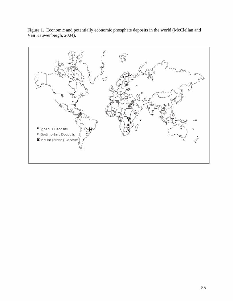
55

Figure 1. Economic and potentially economic phosphate deposits in the world (McClellan and Van Kauwenbergh, 2004).

56

Session III

Changing Landscapes: Drivers & Trends for

Production Agriculture

Session Chairs:

Lori Berger, CA Specialty Crops Council Ben Faber, UCCE, Ventura County

57

Sustainability Landscape: Practices AND Performance

Andrew Arnold, MS, Senior Consultant SureHarvest, 201 Needham Street, Modesto, CA 95354

Ph/fax: (209) 238-9556 www.sureharvest.com ABSTRACT The discussion of sustainable agriculture has gone from "what is it?" to "how do we do it?" as the agri-food chain continues to address economic, environmental and social issues. With new retail and foodservice pressures on suppliers to address sustainability in their operations, we are now in an era for production agriculture to look closely at their business operations through a “sustainability lens.” Early adopters of sustainable practice programs have been able to document adoption of practices along a sustainability continuum to benefit individual growers and, collectively, their crop sector. The next generation programs are now starting to implement quantitative performance metrics to better understand and measure resource management. The Stewardship Index for Specialty Crops is a multi-stakeholder initiative to develop a system for measuring sustainable performance throughout the specialty crop supply chain. The project is developing a suite of outcomes-based metrics to enable operators at any point along the supply chain to benchmark, compare, and communicate their own performance. The metrics results will then allow operators to better understand the relationship between practices and results. The Stewardship Index is not seeking to provide standards, but instead provide a yardstick for measuring sustainable outcomes. In the future, the project may also provide tools and resources to help specialty crop companies advance sustainability goals.

58

Return of the King: It’s Cotton Again in 2010!

Roger A. Isom Executive Vice President, California Cotton Ginners and Growers Associations

& President/CEO, Western Agricultural Processors Association 1785 N. Fine, Fresno, CA 93727

P: (559)252-0684 F: (559)252-0551 Email: roger@ccgga.org ABSTRACT After years of double digit declines due to decreased water availability, a huge influx of dairies and the corresponding conversion to silage and feed crops that go with it, as well as the tremendous conversion to permanent crops like almond and pistachios, cotton is marked to make a tremendous comeback in 2010. With only slightly more than 190,000 acres in 2009, early estimates for 2010 have cotton at somewhere between 300,000 and 400,000 acres! Some growers who got out of the cotton business four or five years ago are taking a look once again. Why the turn around? While we will never see the heyday we once enjoyed in California when we grew 1.6 million acres, many factors are contributing to the return of King Cotton! The end to the unrelenting dairy growth in the San Joaquin Valley, the drop off in nut tree plantings, softening of other competing commodity prices, and the introduction of “roundup ready” pima variety all have helped to heighten the interest in growing cotton in 2010. Coupled with what looks to be incredible fiber prices in 2010, “It’s Cotton Again in 2010”.

59

Session IV

Water Management

Session Chairs:

Larry Schwankl, UCCE, UC Davis David Goorahoo, CSU, Fresno

60

Deficit Irrigation Management Strategies and the Influence of Extended Maturation in Winegrape on Fruit Yield and Quality

Terry L. Prichard, Water Management Specialist

Dept of Land, Air and Water Resources-Hydrology UC Davis 2101 E. Earhart Avenue, Ste 200, Stockton, CA 95206

(209) 953-6120 tlprichard@ucdavis.edu

Introduction Deficit irrigation practices in winegrape have served to improve fruit quality at the cost of decreased yields. The practice of extended ripening, essentially extending the season or delaying harvest until certain flavors are obtained depresses yields through fruit dehydration. When extended maturation became more common in the early 2000’s it was presumed that deficit irrigation and extended ripening were synergistic in causing increased risk for crop reduction and potentially a reduction in fruit quality. In 2004 a field research trial was began to evaluate the effects of deficit irrigation and extended ripening on employed to mitigate vine health, fruit yield and quality of Syrah winegrapes. Of importance was the evaluation of practices yield loss and changes in fruit quality due to deficit irrigation and extended ripening practices. Methods and Materials

A Syrah vineyard using FPMS clone 6 on SO4 rootstock established in 1998 were used in this trial. The site is located near the town of Galt, California. Vine and row spacing is 5 and 11 feet, respectively. Vines are trained to Livingston Divided Canopy (LDC) and are shoot-positioned. The site has a moderate water-holding capacity, increasing in “stoniness” with depth. The well water supply is of good quality delivered via a drip irrigation system. The drip irrigation system was designed and installed to facilitate independent water delivery to individual 32 plots. A plot consists of twenty vines in each of three adjacent vine rows. Data were collected from the 16 central vines located in the central row of the three treatment rows. The experimental design is a randomized complete block, split-split-plot design with four replications of each of three irrigation strategy treatments. The total experimental area is about 2.4 acres Shoot thinning was utilized each year to remove non-productive shoots in all plots. Irrigation Strategy Treatments Irrigation strategies chosen include full potential water use (I-1) and 2 deficit irrigation approaches. Both deficit approaches relied on a level of water stress [-14 bars midday leaf water potential (MDLWP)] to occur prior to the initiation of irrigation. After the leaf water potential threshold was reached, irrigation volume was based on (1) land surface shaded at noon to determine a crop coefficient (Kc), (2) the evapotranspiration reference (ETo) using the Lodi CIMIS station #166, and (3) a 50% regulated deficit irrigation level (RDI). The relationship between land surface shaded at midday and Kc was developed by Larry Williams at the Kearney Ag Center using grapevine in a weighing lysimeter. Essentially, shaded area × 1.7 × ETo × RDI % = irrigation volume applied. Treatment I-3 received

61

50% on a weekly irrigation schedule until harvest of all maturity treatments. Treatment I-2 was irrigated like I-3 until 19º Brix (21 ºBrix in 2005) was reached. At that time, the irrigation volume was increased to 100% based on the canopy size and the current ETo. Irrigation was the same for all plots in the experimental area during establishment of the trial in the 2003 season; with treatments imposed 2004 – 2008. Fruit Maturation Treatments Maturity treatment targets were 24º, 26º, and 28 ºBrix (B-24, B-26 and B-28). Harvest date was determined by sampling berry Brix of each treatment. When the berry samples indicated the Brix treatment level was near, harvest was scheduled for the next day. Fruit maturation treatments were imposed from 2005 through 2008. Crop Load Treatments Crop load treatments were varied by the number of 2-bud spurs on each vine. The 14-spur treatment (S-14) resulted in 5.6 primary buds per foot of row and 0.51 buds per square foot. The 18-spur treatment (S-18) resulted in 7.2 buds per foot of row and 0.65 buds per square foot. The 18-spur treatment resulted in about a 28% increase in buds over the 14-spur treatment. Crop load treatments were imposed 2005-2008 by splitting the fruit maturation treatments plots. Results and Discussion

Three levels of fruit maturity were compared across three different irrigation strategies in a region III/IV Syrah vineyard during 2004 through 2008. Data presented are from years 2005 through 2008 since the long term effects of water deficits are of greatest interest. Significant differences in level of water stress were found between all treatments as measured by seasonal average midday leaf water potential each year. The average levels of water stress within irrigation treatments were similar each year. Irrigation treatment I-2, received an additional 4.0 inches of water at 19 ºBrix in contrast to treatment I-3. This strategy improved vine water relations significantly from increased water application through the remainder of the season. Water consumption was also significantly different among all irrigation treatments. The applied water varies by year as a function of climatic conditions during the season and different amounts of stored moisture at the beginning of the season. Consumed water volumes were similar within irrigation treatment between years. The deficit irrigation treatments I-2 and I-3 consumed 68% and 53% of the full potential consumptive use treatment I-1as an average of years 2005 through 2008. Both the deficit irrigation treatments resulted in higher water use efficiency compared to the full water treatment. Water-use efficiency, whether using applied water or consumed water vs. yield, resulted in a linear relationship. Yield Significant yield reductions occurred with deficit irrigation and extended maturation. Yield reductions, compared to full water (I-1) treatment, were: I-2 at 23% less yield and I-3 at 36% less. The mitigating effect of additional irrigation at 19 ºBrix (I-2) was to reduce yield loss due to deficit irrigation. The deficit irrigation treatment I-2 received 4.0 inches

62

of irrigation water more than the I-3 vines. However, the relationship between yield and water consumption remains linear (Figure 1). When yield is plotted as a function of water consumption (Figure1), it is a strong linear relationship with a R-squared statistic of 99.9%. Figure 1.

Yield as a function of water consumption Syrah 2005-2008 Galt

y = 0.4868x + 4.7188R2 = 0.9988

10

12

14

16

18

20

22

24

15 20 25 30 35 40

Water Consumption (inches)

Yiel

d (lb

/vin

e)

Yield component analysis using simple regression revealed fruit load differences explain 74.4% of the differences in yield while berry size explains 20.1%. The same irrigation treatments were imposed in the 2004 through the 2008 season. Water deficits in I-2 and I-3 were responsible for the decreased cluster number and fruit load. The number of clusters per vine was significantly reduced by 18 % in the continual deficit treatment 1-3 when compared to the other two treatments. Irrigation treatment I-2 cluster number was also significantly reduced from the full water treatment (I-1) by 7%. Significant yield reductions were also found between maturity (Brix) treatments across irrigation and spur treatments (Figure 2). Figure 2 illustrates the effect of water consumption upon yield combined with the change in yield due to extended maturities (or Brix treatments). This figure can be used to visualize the change in yield, as a result of different maturities across irrigation treatments. An example: consider the lowest irrigation level (I-3) where the effect of a 26 to 24 Brix maturity change would result in a 27% yield gain.

63

Figure 2.

Yield as a function of water consumption and harvest maturity% change from 26 Brix

101214161820222426

15 20 25 30 35 40

Water Consumption (inches)

Yiel

d (lb

/vin

e)

Overall

B-24

B-26

B-28

+27%+10% +11%

-12%-7%-6%

The average yield reduction from B-24 to B-26 was 10% while B-26 to B-28 was 18%. The yield reduction was primarily due to reduced berry size. Figure 3 illustrates the effect of berry size on yield at the different irrigation levels. It is a fairly linear change in berry size from B-24 to B-28 maturities. Figure 3.

Yield as a function of consumptive water use and berry size change from B-26 treatment

0.4

0.6

0.8

1

1.2

1.4

1.6

1.8

15 20 25 30 35 40Consumptive Water Use (in)

Ber

ry S

ize

(g/b

erry

)

B-24B-26B-28

+7% +7% +7%

-10% -8% -8%

The mitigating effect of adding crop load by pruning to 28% more spurs was to increase yield by 16% across all irrigation and Brix treatments. Figure 4 illustrates the relationship between water consumption and yield as the spur number changes. As the spur number increases from 14 to 18 per vine the yield increases 17% in the mid level irrigation treatment while it increases 21% in the full irrigation treatment.

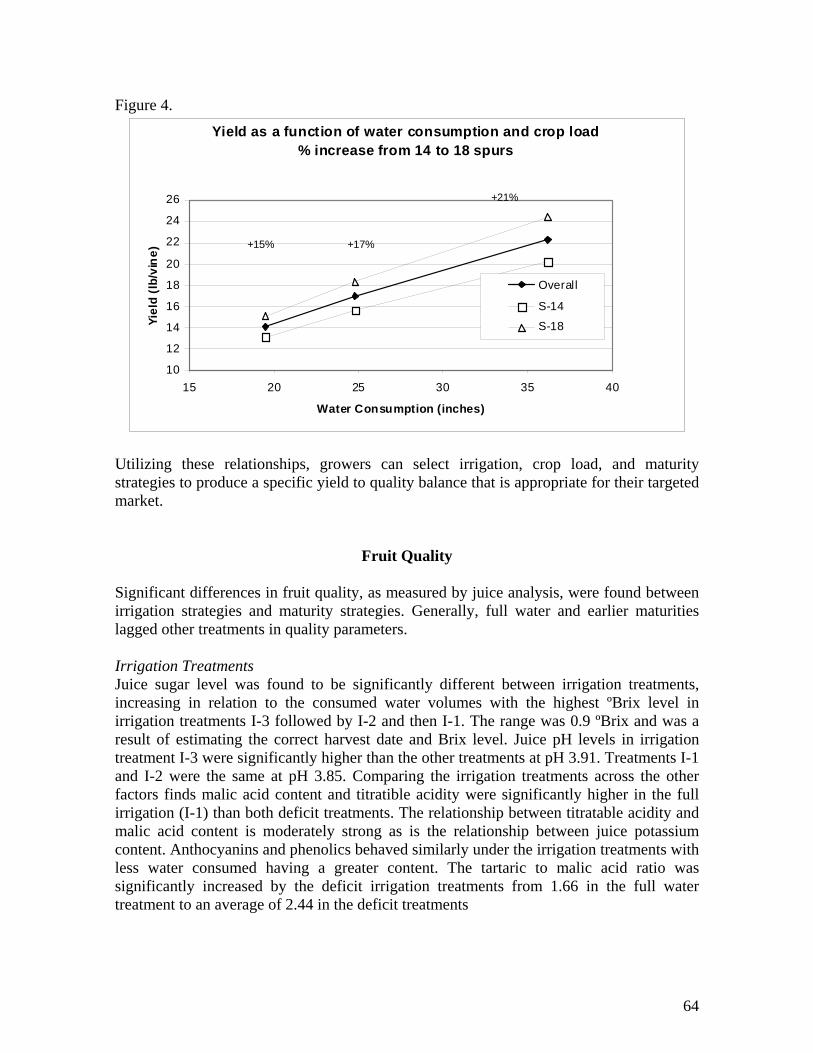
64

Figure 4.

Yield as a function of water consumption and crop load% increase from 14 to 18 spurs

10

12

14

16

18

20

22

24

26

15 20 25 30 35 40

Water Consumption (inches)

Yiel

d (l

b/vi

ne)

Overall

S-14

S-18

+15% +17%

+21%

Utilizing these relationships, growers can select irrigation, crop load, and maturity strategies to produce a specific yield to quality balance that is appropriate for their targeted market.

Fruit Quality

Significant differences in fruit quality, as measured by juice analysis, were found between irrigation strategies and maturity strategies. Generally, full water and earlier maturities lagged other treatments in quality parameters. Irrigation Treatments Juice sugar level was found to be significantly different between irrigation treatments, increasing in relation to the consumed water volumes with the highest ºBrix level in irrigation treatments I-3 followed by I-2 and then I-1. The range was 0.9 ºBrix and was a result of estimating the correct harvest date and Brix level. Juice pH levels in irrigation treatment I-3 were significantly higher than the other treatments at pH 3.91. Treatments I-1 and I-2 were the same at pH 3.85. Comparing the irrigation treatments across the other factors finds malic acid content and titratible acidity were significantly higher in the full irrigation (I-1) than both deficit treatments. The relationship between titratable acidity and malic acid content is moderately strong as is the relationship between juice potassium content. Anthocyanins and phenolics behaved similarly under the irrigation treatments with less water consumed having a greater content. The tartaric to malic acid ratio was significantly increased by the deficit irrigation treatments from 1.66 in the full water treatment to an average of 2.44 in the deficit treatments

65

Brix Treatments The ºBrix treatment targets were 24, 26, and 28 ºBrix. The actual averages were 24.2, 25.6, and 27.3. However, for year-to-year continuity the target ºBrix levels are used in this report. Comparing the ºBrix treatments across the irrigation and spur treatments finds a significant positive (increasing) relationship between ºBrix treatments and pH; and a negative (decreasing) relationship with titratible acidity as a function of increasing ºBrix. Malic acid content was significantly lower in the deficit treatments when compared to the full water treatment. Tartaric acid content was significantly higher in the B-28 treatment when compared to the B-24 and B-26 treatments. Malic acid contents were not significantly different; however the ratio of tartaric acid to malic acid was to be higher in the deficit treatments. Anthocyanins and phenolics behaved similarly under the irrigation treatments with less water consumed, having a larger content than the I-1 treatment. Spur Treatments No significant differences were found between any measured juice parameter. Summary

Deficit irrigation techniques and extended maturation (or delayed harvest) strategies each reduce yield over time as a result of decreased fruit load from fewer clusters and smaller berries while extended maturation decreases berry size. When comparing a full water irrigation strategy (I-1) to the continual deficit treatment (I-3) the yield reduction was 36%. The deficit strategy I-2 significantly improved yield over the continual deficit treatment I-3 however the increased applied water resulted in a predicted increased yield by preserving berry size. The improvement in yield I-2 over I-3 occurred while changes in most juice parameters were unchanged. The strategy of increasing fruit load by pruning to 30% more primary buds resulted in a 16% average yield boost while vine balance seems not to have been affected; no significant delay in harvest was found; and changes in Juice components were not significant. Utilizing water deficits, extended maturity harvest, and leaving more spurs at pruning to each has a distinct effect on yield and fruit quality. Any combination of these strategies should be carefully considered and compared to the quality changes and always compared to the value of the crop.

66

Regulated Deficit Irrigation for California Pistachio

Dr. David A. Goldhamer and Mr. Robert Beede Water Management Specialist and Kings County Farm Advisor

University of California Cooperative Extension The pistachio industry in CA is relatively young compared with other nut crops, including almonds and walnuts. Also, the industry tends to be dominated by a few large, growers and processors. They have readily embraced progressive production practices, including drip or microsprinkler irrigation, which is now the dominant form of irrigation industry-wide. As such, CA pistachio growers have a relatively high level of control of the distribution uniformity, timing, and amounts of applied water. Moreover, California pistachio growers were very quick to adopt useful research results on the impact of water stress on yield and crop quality. In terms of the later, pistachio is distinguished by more quality components than other nut crops. These include not only alternate bearing but embryo abortion; nuts that have full size hulls and shells but where the kernels die prematurely or don’t fill at all. Also, endocarp dehiscence (shell splitting) is required to produce the highest value nuts. Closed shell nuts at harvest cannot be marketed as snack food, which is the largest market for pistachios. Finally, the percent removal of filled nuts by mechanical shaking also impacts harvest yields. All of these yield components can be negatively impacted by water stress. Stages of Development The reproductive growth in pistachio trees can be divided into three stages based upon the development of the nut component parts: the hull+shell and the kernel. The development pattern of the nut components is shown in Fig. 1. The hull+shell grow rapidly from late April through mid May when full size is attained. This period is referred to as Stage 1. However, the feniculous, which will eventually evolve into the kernel, does not begin to grow until early July. Thus, from mid May through early July, the primary growth activity in the nut is thickening of the shell. Thus, there is a relatively low rate of dry matter accumulation in the nut from mid May through early July period, which is known as Stage 2, Rapid growth of the kernel begins in early July and remains so as harvest is approached. The biofix for this period, which is known as Stage 3, is the appearance of a distinct green color in the feniculous. Research (Spann et al., 2009) has identified the concomitant vegetative growth associated with these stages and their eventual importance as locations for fruiting positions. Early Vegetative and Reproductive growth; Growth Stage 1. Shoot growth occurs simultaneously with the current season reproductive growth (swelling buds that will form the crop) as well as with embryonic (inflorescence primodia) bud development for the following season’s crop from late April thru mid May in the northern hemisphere. Lateral inflorescences in the leaf axils are borne on shoots with generally a single apical vegetative bud. Buds differentiate in April, May and June, remain quiescent from July-September, and resume differentiation in October.

67

There are two types of shoot growth; preformed or neoformed. All components of a preformed shoot are differentiated in the dormant bud whereas in neoformed growth, some differentiation of its component parts can occur during the growing season. Most of the buds found on preformed growth are reproductive; there are very few lateral vegetative buds on preformed shoots. Most of the vegetative growth occurs from terminal buds. Preformed shoots tend to be short compared with neoformed shoots which are longer. This longer shoot growth is undesirable because it tends to be weak and hangs down in the orchard rows, making management and harvest difficult. For these reasons, grower typically remove these shoots on mature trees by pruning during the dormant season. However, long shoot growth may be desirable in young, developing trees to ensure the most rapid development of the tree canopy. Reproductive buds swelling begins in March. By mid April, there are 100-300 flowers per rachis. Pollination and fruit set occur at this time. There are generally 20-25 developing fruit per rachis and they grow rapidly, with the hull+shell attaining full size by about mid May. This event also generally coincides with a stiffening of the shell. Lag phase of reproductive growth; Growth Stage 2. From mid May through early July, the only activity in the nut is thickening of the shells, often called lignification. However, dry matter accumulation during this growth phase is low relative to the preceeding (Stage 1) and succeeding (Stage 3) periods. There may also be some additional shoot growth in late May. Reproductive buds that will form the following season’s fruit continue to differentiate through June. Sometimes there is an additional vegetative flush of growth in late June. Rapid kernel development; Growth Stage 3. This phase is characterized by the resumption of a high rate of dry matter accumulation in the nut due almost entirely to the rapid growth of the kernel. Within a matter of a few weeks, the kernel will entirely fill the nut cavity and begin to exert pressure on the shell. Shell splitting is primarily due to this expansion of the kernel (Polito and Pinney, 1999). Shell splitting generally begins in early August. At this time, the hull begins to breakdown, changing from turgid tissue that’s tightly bound to the shell to a papery, loosely connected covering that can easily be peeled from the shell. During Stage 3, leaves on the same shoot as developing fruit sometimes become yellow and defoliate. This is though to be the consequence of translocation of resources from the leaves to the fruit. A certain percentage, generally 10 to 30%, of the nuts do not fill. These are known as “blanks” or “aborted” nuts. With the former, there is no evidence of any development of the embryo whereas with the latter, the embryo development was aborted. The term “blanking” is sometimes used to describe both phenomena. The hulls of these nuts do not breakdown as with the filled nuts. They also are much more difficult to remove from the tree with mechanical shaking at harvest, resulting in a high percentage remaining in the tree.

68

Postharvest From harvest to the onset on defoliation, there is very little outward appearance of tree activity. Following the removal of fruit, reproductive bud differentiation resumes and continues through October. Trees generally defoliate in mid to late November due to leaf senescence, which is accelerated by low temperatures. Responses to Water Deficits Pistachio has a well deserved reputation of being drought tolerant. Behboudian et al. (1986) found measurable photosynthetic activity in the leaf even when leaf water potential was in excess of -5 MPa. The concluded that this was due to the fact that pistachio trees had a turgor pressure of about 3 MPa even when the leaf water potential was -6 MPa; a higher value that for even other xerophytes. Walker et al. (1988) also found that pistachio could maintain high turgor even with high soil salinity levels. Lin et al. (1981) found high photosynthesis and stomatal conductance in various pistachio species under severe stress. However, they concluded that this was primarily due to an extensive rooting system rather than xerophytic morphologic characteristics. Germana (1997) found that with unirrigated trees, P. atlantica had transpiration rates about three times higher than P. terebinthus. They pointed out that pistachio trees can transpire water at rates far higher than those normally found in mesophytes and that carbon assimilation with limited water supplies was much higher than other fruit crops, such as apple, peach, plum, cherry, citrus, and almond. Thus, pistachio is somewhat of a paradox; it has the ability to transpire at an extremely rapid rate, in part, due to the fact that its leaves are “isolaterals” with the upper and lower sides similarly structured with almost identical stomatal density and conductance but is also extremely drought tolerant. Stage 1. Spann et al. (unpublished) tested RDI regimes that imposed water deficits of about -1.6 MPa midday shaded leaf water potential on mature trees of “Kerman” on PG1, Atlantica, and UCB rootstocks during Stage 1 and both Stage 1 and Stage 2. They found that especially for the “short” shoots, those that are characterized as preformed growth, full elongation occurred by about the third week of April; well before the onset on Stage 2. There were generally no reductions in this short shoot length due to these early season water deficits (Fig. 2). However, stress during both Stages 1 and 2 significantly reduced the growth of the “long” shoots; the neoformed growth (Fig.2). Spann et al. (unpublished) concluded that the stress prevented the short shoots from growing into long shoots. This did not decrease the number of fruiting positions since they are located mostly on the short shoots. Indeed, they found no differences in fruit load, fruit size, and yield between these RDI regimes and the fully irrigated Control. They attribute this to the fact that most of the fruit was borne on the preformed growth and that reducing neoformed growth was actually beneficial in commercial since it must be pruned. Beede et al. (2004) concluded that water and pruning costs are about 30% of the total for California pistachio growers and thus, the reductions in consumptive use and pruning attributed to the early season stress would likely increase grower profit. Spann et al. (unpublished) found that with the UCB rootstock, they found some reduction in the total number of growing shoot per tree with both Stage 1 and Stage 2 stress and cautioned that this could reduce future yield if it were

69

to continue for a number of years. This confirmed earlier work of Goldhamer et al. (1987) that stress-related reductions in fruit load were primarily due to the reduction in the initiation of short shoots rather than potential or actual nuts per rachis.

Goldhamer and Beede (2004) imposed dryland conditions during Stage 1 with “Kerman” on Atlantica rootstock. They found that nut size was reduced by 6.1% relative to a fully irrigated Control but that shell splitting was increased by 14.0%. They theorized that the stress impacted shell growth more than kernel growth, resulting a greater splitting percentage. Since no other yield components were significantly affected, they reported slightly better total kernel yield of marketable product (split nuts) with Stage 1 stress. More recent research has confirmed that shell splitting can be increased with Stage 1 stress but at the expense of nut size (Goldhamer et al, 2005). Thus, the decision to use this RDI regime would depend on whether the grower had a severe problem with the production on closed shell nuts. Closed shell nuts can be as low as 5% of the harvested nut load and a high as 60%. Additionally, Stage 1 stress not only increased shell splitting but it increased the shell opening; the distance between shell halves at the distal end of the nut. This can result in the shell detaching from the kernel during commercial nut processing and while the loose kernels can bring a lower price than split nuts. Stage 2. Goldhamer and Beede (2004) evaulated an array of RDI treatments that imposed either dryland, applied water at 25% ETc, and applied water at 50% ETc during Stage 2 on mature “Kerman” on Atlantica rootstock under the high evaporative demand conditions of the western San Joanquin Valley in California. These Stage 2 deficit irrigation treatments were coupled with different postharverst regimes. They found that none of the Stage 2 stresses significantly reduced individual nut weight although there was a trend toward lighter nuts when Stage 2 irrigation was totally eliminated. One of these Stage 2 dryland treatments, when coupled with irrigation at 25% ETc postharvest, significantly reduced the yield of split nuts. Goldhamer and Beede (2004) concluded that Stage 2 was, indeed, a stress tolerant period and recommended an RDI regime that irrigated at 50% ETc during Stage 2. Sedaghati and Alipour (2006) reported that a June deficit irrigation of 20% less than the Control doubled early splits while a July deficit of 35% increased early splits by 30%. Early splits are nuts that split well before the onset of normal shell splitting. These nuts are not commercially viable. Moreover, they are susceptible to fungal diseases that can eventually result in Aflatoxin contamination. Doster and Michailides (1995) observed that avoiding water stressing stress during mid-May significantly decreased the incidence of early splits. Stage 3. Stress imposed during Stage 3 can have a dramatic negative impact on virtually all the yield components of pistachio. Goldhamer and Beede (2004) imposed a dryland treatments during Stage 3 and found that this reduced individual kernel weight by 10.6%, increased the sum of blanking and kernel abortion in the total tree nut load by 22.7%, and increased the production of closed shell nuts by 175%. Somewhat remarkably, the Stage 3 dryland treatment had no affect on total tree nut load. However, the yield of split nuts was reduced by 62.6%.

70

Goldhamer et al. (1991) reported that withholding irrigation during the first half of Stage 3, which reduced consumptive use by 320 mm, had no significant impact on shell splitting but increased the number of filled nuts left in the trees after mechanical shaking by 119%. On the other hand, dryland conditions during the last half of Stage 3 (a 200 mm reduction in consumptive use) both increased the production of closed shell nuts at harvest by 31.6% and the number of filled nuts retained on the tree after mechanical shaking by 50.0%. They concluded that Stage 3 was the most stress sensitive period of the season in pistachio. Of the numerous pistachio yield components, Goldhamer and Beede (2004) remarkably found that tree nut load was unaffected by any of the nine deficit irrigation treatments they imposed, including dryland conditions during Stage1, Stage 2, Stage 3, and postharvest and the various Stage 2 and postharvest stress combinations. When averaged over the last two years of their four year study, tree nut load ranged from 10900 to 12300 with the near fully irrigated Control being 11500 nuts per tree. This suggests that there was enough preformed shoot growth very early in the season, even with Stage 1 dryland conditions, to produce the number of nodes (fruiting positions) necessary to support a full crop and that stored winter rainfall (200 mm per year) was sufficient to support this growth. This ability of the pistachio tree to produce equal fruit loads under a variety of stress regimes highlights the importance of the preformed shoot growth from mid April to mid May; a period when trees would normally rely on stored winter rainfall rather than irrigation. Indeed, the early work of Spiegel-Roy (1977) found that 54 to 163 mm of annual precipitation was enough for dryland trees to differentiate enough flower buds to obtain appreciable yields. Water Production Function The optimal RDI regime suggested by Goldhamer et al. (2004) employs stress during Stage 2 and postharvest to achieve the same production as fully irrigated trees while reducing the consumptive use of water. We tested this approach in numerous field trials in the San Joaquin Valley of California. The results of these experiments are summarized in the production function shown in Fig. 3. While there is appreciable scatter in the data, it suggests that a plateau in the yield of marketable product is achieved with 10 to 20% less consumptive use than potential ETc. Said another way, reducing consumptive use by up to 20% can be generally be achieved with a plus or minus 10% impact on the yield of marketable product. This occurred with both Altantica and PG1 rootstocks. It should be emphasized that that a 10 to 20% reduction in ETc would translate into a higher percentage reduction in applied water. For example, if ETc was 1100 mm per of which 300 mm was effective rainfall, then applied irrigation water would have been 800 mm. A 15% reduction in ETc would reduce consumptive use by 165 mm; about a 21% reduction in applied water.

71

Suggested RDI Regimes Based on the assumption that Stage 2 and postharvest are most stress tolerant, Stage 1 is intermediately tolerant, and Stage 3 is least tolerant, one can develop an array of drought irrigation strategies based on meeting certain percentages of ETc during these periods (Table 1). The percentage amounts for each period vary depending on the available water supply. It should be pointed out that these recommendations are based on experimental results of applied water amounts generally above about 750 mm; nobody has tested RDI regimes below this amount. Thus, the suggested regimes for water supplies below 750 mm are our best estimate of what would result in optimal tree performance, again based on the stress sensitivities of each growth stage. Since the contribution of soil moisture to ETc is difficult to determine, especially early in the season, which makes RDI management by irrigating at certain percentages of ETc problematic, an alternative is to use a plant based indicator of tree water stress, such as the pressure chamber. The current state of the art in plant-based measurements is the pressure chamber. In the studies cited above, Goldhamer et al. (2005) found that midday shaded leaf water potential during Stage 1, Stage 2, and postharvest did not exceed -1.8 to -2.0 MPa. They choose to use shaded leaf water potential because it is not complicated by having to bag the leaves, as is the case with stem water potential measurements. Moreover, they found a good correlation between midday shaded leaf water potential and stem water potential (R2=0.948) as shown in Fig. 4. They also suggest that fully irrigated, mature pistachio trees grown under high evaporative demand conditions should have midday shaded leaf water potential values for Stage 1, Stage 2, Stage 3, and postharvest of -0.7 to -0.8 MPa, -0.8 to -1.0 MPa, -1.0 to -1.1 MPa, and -1.0 to -1.2 MPa, respectively. One factor that complicates taking water potential measurement on pistachio leaves is that at the onset of gas injection into the chamber, exudates, presumably from the phloem, appear at the cut end of the petiole. These can interfere with identifying the instant xylem fluids appear. One approach to eliminating this problem is to use a cotton swap to soak up these exudates prior to the appearance of the xylem fluid. Another approach to eliminating this problem uses blotting paper positioned at the cut end of the petiole that absorbs only xylem fluid but excludes what they called the “turpentine,” presumably the other interfering fluids. A third approach is to not uses individual leaves but small, interior shaded spurs that may have one to four leaves. The procedure involves covering the spur with a damp cloth just prior to excision. A few mm of bark is removed at the cut end with either a small knife or one’s thumbnail. The entire spur is placed in the chamber after the cloth is removed and the reading is taken. It’s quite easy to identify the appearance of the xylem since the no interference of phloem exudates and the cross-sectional area of view is larger than the leaf petiole. Goldhamer et al. (unpublished) found a good correlation between spur water potential and midday shaded leaf water potential (R2=0.944) as shown in Fig. 5. The slope of the relationship is about unity but the y intercept indicates that the spur water potential differs from the shaded leaf water potential reading by about -0.7 MPa.

72

One pistachio grower in California has observed that there is little need to irrigate male trees at to obtain full ETc since their only role is to supply pollen very early in the season. He suggests that irrigation can be eliminated or substantially reduced after Stage 1 with no negative impact on the subsequent season’s pollen formation. This can be accomplished relatively easily with microirrigation systems. References Beede, R. H, C. E. Kallsen, M. W. Freeman, L. Ferguson, B. A. Holtz, K. M. Klonskey, and R. L. DeMoura. 2004. Sample costs to establish and produce pistachios. Univ. of CA Coop. Extn. Publ. PI-SJ-04. 25 p. Behboudian, M. H, Walker, R. R., and E. Torokfalvy. 1986. Effects of water stress and salinity on photosynthesis of pistachio. Sci. Hort. 29:251-261. Doster, M. A. and T. J.Michailides. 1995. The development of early split pistachio nuts and their contamination by molds, aflatoxins, and insects. Acta Horticulturae 419:359-364. Germana, C. 1997. The response of pistachio trees to water stress as affected by two different rootstocks. Acta Horticulturae 449:pages unknown Goldhamer, D. A., Kjelgren, R., Beede, R., Moore, J. M., Lane, J., Menezes Jr., J., and G. Weinberger. 1984. Physiological response of pistachio to severe water stress. In: Annual Report. Crop Year 1983-1984. California Pistachio Industry, Fresno, CA, pp. 44-47. Goldhamer, D. A., Phene, B. C., Beede, R., Sherlin, L., Mahan, S., and D. Rose. 1987. Effects of sustained deficit irrigation on pistachio tree performance. In: Annual Report. Crop Year 1986-1987. California Pistachio Industry, Fresno, CA, pp. 61-66. Goldhamer, D. A., Beede, R. H., and S. Fusi. 1991. Effects of deficit irrigation timing on pistachio tree productivity. In: Annual Report. Crop Year 1990-1991. California Pistachio Industry, Fresno, CA, pp. 84-87. Goldhamer, D. A., and R. H. Beede. 2004. Regulated deficit irrigation effects on yield, nut quality and water-use efficiency of mature pistachio trees. J. Hort. Sci. and Biotechnology 79(4):538-545. Goldhamer, D. A., Beede, R.H., Michailides, T. J., Salinas, M., and M. Doster. 2005. Effects of regulated deficit irrigation on shell splitting and nut quality at harvest (second year report). In: Annual Report. Crop Year 2004-2005. California Pistachio Industry, Fresno, CA, pp. 104-106. Sedaghati, N. and H. Alipour. 2006. The effect of different time of irrigation on occurrence of early split (ES) of pistachio nuts. Acta Horticulturae 726:583-586.

73

Spann, T. M, Beede, R. H., and T. M DeJong. 2009. Contributions of short- and long-shoots to yield of ‘Kerman’ pistachio (Pistaca vera L.) In Press. Polito, V. S. and K. Pinney. 1999. Endocarp dehiscence in pistachio (Pistacia vera L.). Internacional Journal of Plant Sciences 160:827-835.

74

Table 1. Suggested RDI strategies for different available water supply senarios from 900 to 300 mm when potential ETc is 1100 mm.

900 mm Available Case

750 mm Available Case

600 mm Available Case

450 mm Available Case

300 mm Available Case

Date

Potential ETc in Period (mm)

Irri. Rate

(% ETc)

Applied Amount

(mm)

Irri. Rate

(% ETc)

Applied Amount

(mm)

Irri. Rate

(% ETc)

Applied Amount

(mm)

Irri. Rate

(% ETc)

Applied Amount

(mm)

Irri. Rate

(% ETc)

Applied Amount

(mm) Apr 16-30 33 100 33 50 16 50 16 25 8 10 3 May 1-15 59 100 59 50 30 50 30 25 15 10 6 May 16-31 91 50 45 25 23 25 23 25 23 10 9 Jun 1-15 122 50 61 25 31 25 31 10 12 10 12 Jun 16-30 137 50 68 25 34 25 34 10 14 10 14 Jul 1-15 128 100 128 100 128 75 96 10 13 10 13 Jul 16-31 123 100 123 100 123 75 93 75 93 50 62 Aug 1-15 124 100 124 100 124 75 93 75 93 50 62 Aug 16-31 100 100 100 100 100 75 75 75 75 50 50 Sept. 1-15 83 100 83 100 83 75 62 75 62 50 42 Sept. 16-30 56 100 56 25 14 25 14 25 14 10 6 Oct 1-15 35 100 35 25 9 25 9 25 9 10 4 Oct 16-31 19 100 19 25 5 25 5 25 5 10 2 Nov 1-15 10 100 10 25 2 25 2 25 2 10 1 Total 1121 946 722 583 438 284 Irrigations per season 30 25 19 16 12 8

Typical microsprinkler application Appl. Rate 1.47 ft3/hr Tree Spacing 289 ft2 Ppt. Rate 0.01 ft/hr Ppt. Rate 0.06 in/hr Amt. per Irr. 1.47 in/24hr Amt. per Irr. 37.2 mm/24hr

75

Fig. 1. Time course development of dry matter accumulation in pistachio nuts illustrating

the three growth stages. Vertical bars are plus and minus one standard error of the mean.

0.000

0.002

0.004

0.006

0.008

0.010

0.012

0.014

0.016

0.018

0.020

Apr 16 May 1 May 16 May 31 Jun 15 Jun 30 Jul 15 Jul 30 Aug 14 Aug 29

Frui

t Dry

Mat

ter A

ccum

ulat

ion

Rat

e (g

/d)

Stage 2 Stage 3Stage 1

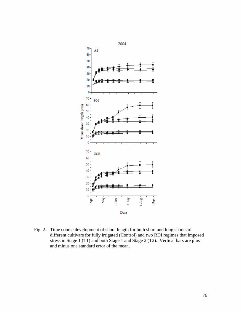
76

Fig. 2. Time course development of shoot length for both short and long shoots of

different cultivars for fully irrigated (Control) and two RDI regimes that imposed stress in Stage 1 (T1) and both Stage 1 and Stage 2 (T2). Vertical bars are plus and minus one standard error of the mean.

77

Fig. 3. Production function for developed using RDI strategies that imposed stress during Stages 1, 2,

and postharvest only for at least four year duration. Eight studies from US and Europe met this criterion and are presented. Dashed line shows linear regression from full yield, full ETc through zero yield, 7% ETc; the level considered necessary for tree survival.

40

50

60

70

80

90

100

110

40 50 60 70 80 90 100 110

Consumptive Use (ETc) Relative to Fully Irrigated Trees

Yie

ld o

f S

plit

Nu

ts R

ela

tive t

o F

ully I

rrig

ate

d T

ree

Kettleman City, CA, Atlantica

Madera, CA, PG1

Parlier, CA, Atlantica

Parlier, CA, PG1

Lost Hills, CA, Atlantica

Madera, CA, Atlantica

Turkey, Uzun

Spain, Terebinthus

78

Fig. 4. Relationship between midday shaded leaf water potential and midday shaded stem water

potential with linear best fit expression.

y = 1.18x + 0.725R2 = 0.948

0

5

10

15

20

25

30

0 5 10 15 20 25 30

Midday Shaded Stem Water Potential (-bars)

Mid

day S

had

ed

Leaf

Wate

r P

ote

nti

al

(-b

ars

)

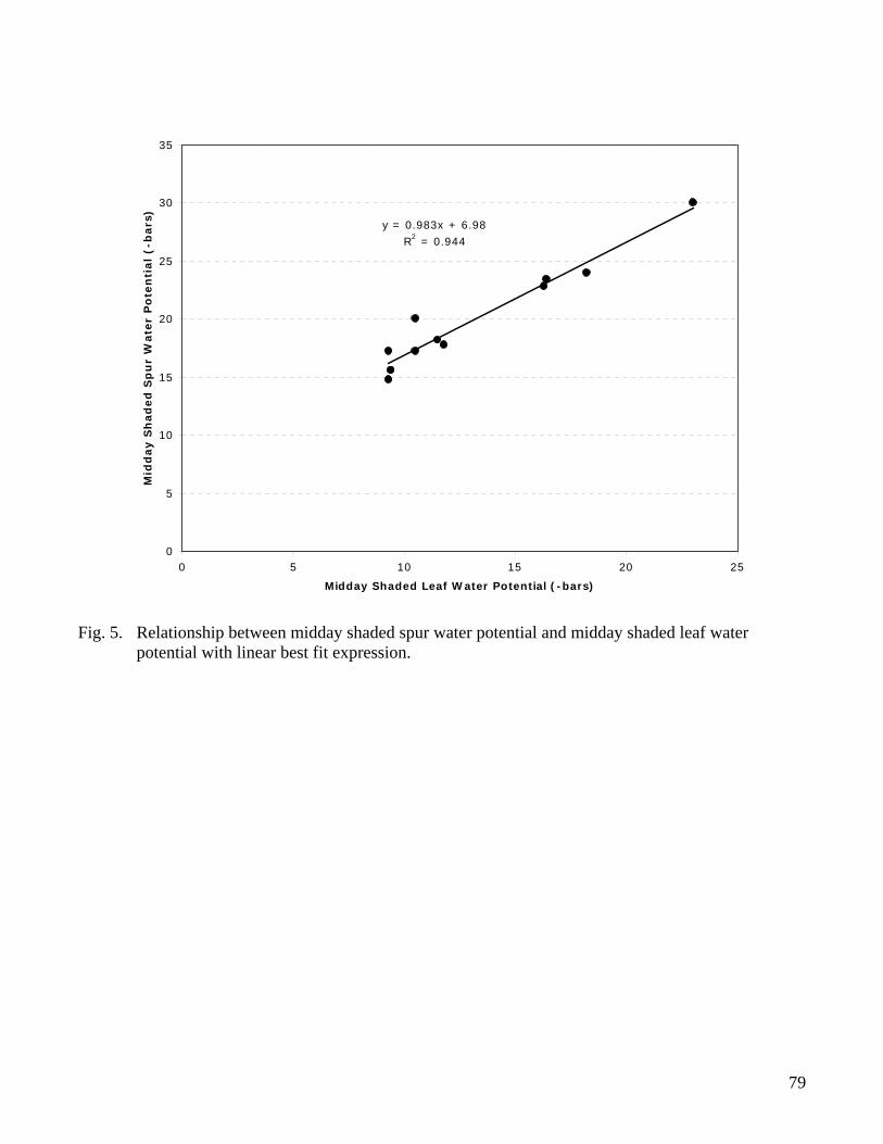
79

Fig. 5. Relationship between midday shaded spur water potential and midday shaded leaf water

potential with linear best fit expression.

y = 0.983x + 6.98R2 = 0.944

0

5

10

15

20

25

30

35

0 5 10 15 20 25

Midday Shaded Leaf Water Potential (-bars)

Mid

day S

had

ed

Sp

ur

Wate

r P

ote

nti

al

(-b

ars

)

80

Irrigating Corn with Limited Water Supplies

Carol Frate, Farm Advisor University of California Cooperative Extension, Tulare County

4437 S. Laspina St., Tulare, CA 93277 phone: 559-684-3300; fax: 559-685-3319; cafrate@ucdavis.edu

Introduction Field corn acreage in California from 2006 – 2008 ranged from 515,000 to 665,000 acres with approximately 75% harvested for silage (8). The Central Valley accounts for 98% of the state’s corn acreage. The Sacramento Valley contains 12% of the acreage, of which roughly two thirds is for grain. (In the past 3 years the percent of the acreage going to grain in the Sacramento Valley ranged from 54% in 2008 to 83% in 2007). The San Joaquin Valley has 86% of the corn acreage, of which 80% is for dairy silage. Some corn varieties are designed specifically for grain production while others are promoted for silage. However, many growers in the state choose “dual purpose” varieties that can be grown for either, enabling the farmer to evaluate the market and decide at the last minute whether to go for grain or silage. The state’s average yield of grain corn for 2006-2008 was just over 5 tons per acre. For that same period the average for silage corn was 26.7 tons per acre (70% moisture). While the emphasis of this paper is on field corn, the information provided should also apply to sweet corn. Corn and Corn Growth Corn is a monocot with the C4 photosynthetic pathway which is more efficient than the more common C3 pathway. C4 plants have higher water use efficiency than C3 plants and are better adapted to hot climates with intense sunlight than C3 plants. Other C4 plants include sorghum, sugarcane, and amaranths. Corn has a relatively small root system compared to sorghum. The majority of the water used by corn will be in the top 2-3 feet of soil. Depending on variety, a corn crop can go from planted seed to grain maturity in as short as 80 days (or less) or as long as 125 (or more) days. Varieties taking longer to mature usually have higher yields. In the southern San Joaquin Valley varieties are usually chosen that take 105 to 120 days to maturity. The longer season varieties would be for single crop grain production planted in March. Silage crops usually follow winter forage and are planted from late April through June and sometimes later. Visually, corn development is divided into the vegetative stage that lasts through tassel and the reproduction stages that include silking, pollination, and grain filling (5). Stress during the vegetative stage (any stress prior to 2 weeks before silking) can slow the appearance of new leaves, reduce leaf area expansion, reduce plant height, and delay crop maturity (9, 15). Stress during reproduction will hasten maturity and reduce yields. Crop Water Use Corn evapotranspiration (ET) estimates for the Central Valley range from 25 to 29 inches, depending on location within the Central Valley, time of planting, and season length for the variety chosen (11). At full canopy, ET is around 0.3 inches/day.

81

General strategies for coping with limited water include deficit irrigation of crops which can be stressed without significant loss of yield or quality, improving irrigation efficiency and/or uniformity, improving crop genetics to develop varieties more tolerant to water stress, or planting other crops. Deficit Irrigation of Corn Deficit irrigation can be defined as the application of water below the (ET) requirements of the crop (3). Deficit irrigation of tree and vine crops has been more successful than on annual crops. Reasons for this include yield determining processes in many fruit trees are not sensitive to water shortage at some stage of development, economic return is often due to quality and not as directly related to ET and biomass production as in many annual crops, and higher value crops often have micro-irrigation systems that enable application of small amounts of water with fine-tuned scheduling (3). What is the impact of irrigating corn below what is needed for maximum ET and does it matter if the stress is throughout the season or at specific times? Considering first season-long deficit irrigation, recognize that biomass production is tightly associated with ET. When ET is reduced from the optimum for a crop, biomass is reduced. From the silage point of view, any loss of biomass reduces yield. In addition silage quality is a concern. Fiber digestibility is a major component of silage quality. Papers reviewed for this presentation did not address if, or how much, water stress affects silage quality. However because the grain is a major component of silage quality, both grain and silage producers have a similar concern: what is the impact of limited water on grain production? Besides biomass reduction, water stress can affect the Harvest Index (HI) which is the fraction of the above-ground biomass that is harvested. To a point, corn can be stressed through the season so that the fraction of grain compared to the total above ground biomass does not decline. However, there is a reduction in yield because total biomass declines even though the percent of the biomass that is grain remains constant (3). Under this scenario, stress gradually increases during the season as the soil water reserve declines and the irrigation water applied is less than optimum ET. If too much stress occurs, then the HI declines. The amount of stress corn can withstand before the HI is impacted depends on soil type and ET demand. Realistically, it would be hard to manage even is a grower was willing to accept the yield decrease. If simply under-irrigating through the season is not a reasonable strategy, is there a time in corn development when water stress can be applied without impacting grain yield? Can an irrigation be skipped or the irrigation interval be extended significantly at a particular growth stage without impacting yield? Most studies demonstrate, and experience has shown, that there is no good time to stress corn. But if water stress is unavoidable, then it is best during the vegetative period up to 2 weeks prior to silk emergence. Stress during this vegetative period has the least impact on grain yield. It can result in shorter corn and may delay the appearance of new leaves and tassels. If water stress is severe, it may negatively impact nodal root development and a dry hard soil surface when brace roots start to grow may impede their development. These smaller root systems may lead to mature plants falling over when the field is irrigated (9). The second least damaging time for water stress is late season during grain fill when it can reduce photosynthesis and reduce movement of carbohydrates into the kernels. The number of kernels is not reduced but kernels are smaller than they would be if plants were well watered. If stress is extreme,

82

kernels can be shriveled. Additionally late season water stress can increase stalk rot leading to higher risk of lodging with subsequent harvest losses. The most important time to avoid water stress is the 2 weeks prior to silking through the 2 weeks following silking. Stress before silk emergence can delay silking relative to pollen resulting in insufficient pollen available for good fertilization. If the stress occurs during pollination, silks may desiccate, preventing pollen germination or the pollen tube from extending down the silk to fertilize each kernel. Kernel abortion can also occur. The result is an ear with reduced number of developing kernels. It has been estimated that severe stress 2 weeks prior to silking can reduce grain yield by 3-5% per day; at silking 3-8% per day; and during the 2 weeks following silking, 3-6% per day (9). Regulated deficit irrigation is not a strategy that is promising for corn as there is no really good time to impose stress. It is also a strategy that would be difficult to implement with furrow or flood irrigation, the most common types of irrigation for corn in the state, because it is hard to regulate the amount of water applied with these systems. Variety Selection Growers can choose from a wide selection of varieties. One characteristic of a variety is the relative days to maturity. Corn varieties grown for silage and planted in May are often “105 day” varieties. Corn planted in March for grain might be 125-day varieties. Generally a grower wants to have a variety that is a long as the climate allows because in general the more days to maturity, the higher the yield. Growers facing a shortage of water, however, may want to consider planting shorter season varieties. In the end, it may be better to have an adequately watered short season corn than a stressed longer season variety. Irrigation systems Because opportunities for reducing the amount of water available for ET are limited without yield loss in corn, improvement in utilizing the water applied is another strategy. Specifically, losses due to deep percolation or runoff must be reduced. Some water needs to drain below the root zone to remove salts but excessive drainage needs to be avoided. Fields and irrigation systems vary due to numerous factors, including soil types, slope, flow rate, and irrigation management. For the purpose of this paper, generalizations have to be made but it is important to realize that the alternatives mentioned need to be evaluated on a specific field with consideration of the performance of the irrigation system currently in use. Finally, the economics of significant changes in irrigation systems and management must be considered but are beyond the scope of this paper. Currently almost all of corn grown in the California is irrigated by surface irrigation, mostly furrow but some flood irrigation is also used. Depending on soil type and system design, these methods can be quite efficient, but often there is room for improvement. Corn roots are not particularly deep or well developed. Most water is taken up from the top 2 feet. Growers are often on a 7 – 10 day schedule. At maximum canopy, ET for corn is about a third of an inch per day. In 10 days, about 3 inches would be needed to refill the profile but many furrow systems would apply 4-6 inches just to get water to the end of the field. With pre-irrigation and irrigations following cultivation, application rates are commonly even higher.

83

For furrow irrigation the management strategy that most improves irrigation efficiency and uniformity is to shorten the irrigation run. If the on-field flow rate remains the same, halving the field length reduces the time needed for water to reach the end of the field by at least 30-40%, usually improves distribution uniformity by 10 – 15%, and often reduces deep percolation by more than half (4). With less time to reach the end of the field, less water is applied. However shortening the field will result in more surface runoff so a way to re-use this runoff water, such as a tail water recovery system, is needed. An example of the impact of shortening a field is found in Table 1. Alternate furrow irrigation can reduce subsurface drainage and runoff. In one study comparing alternate and every-row furrow irrigation in corn on different soil types, yields were equivalent for the two methods (4). With alternate furrow irrigation, 29% less water was applied than was applied with every-row irrigation. Alternate row irrigation has the added benefit of moving salts from the wet furrow across the bed and out of the seed row, which may be of benefit in some situations. However, some studies in different crops have shown a yield reduction with alternate furrow irrigation. Some soils, in particular those that crack across the bed are not very adaptable to alternate furrow irrigation. As always, care must be taken when trying new irrigation methods on a particular field. For many soils, strategies to reduce the amount of applied water would only need to be used on those irrigations following cultivation when infiltration is high. It is common that 6-9 inches (or more) can be applied in a pre-irrigation. In a soil that holds 1 inch of water per foot, this would wet the soil to 6-9 feet, much deeper than corn roots will effectively take up water. Irrigations that follow cultivation can also result in heavy applications of water. Plants are usually small at this stage and their root development limited resulting in much of the water applied not being available to the plants. A major challenge is how to limit the amount of water applied when irrigation occurs after the ground has been cultivated prior to planting or when plants are small. Torpedoes are heavy tube-sahped blocks pulled through furrows to smooth the floor of the furrow, allowing the water to run more quickly to the end of the field. In one study of a pre-irrigation event, torpedoes reduced the amount of water applied on a quarter mile run from 12.9 inches without torpedoes to 9.4 inches on the “torpedoed” furrows. In that same study the water was also monitored at 600 ft. In this case, shortening the field by half would have resulted in an application of 7.1 inches without torpedoes and 4.3 inches with torpedoes (Table 1). Another method to reduce infiltration with furrow irrigation is surge irrigation. With surge irrigation water is allowed to run a certain distance down the field and then the irrigation set is switched to a new set of furrows. While the alternate set of furrows get irrigated, the water in the original set drains. The water is then switched back to the original set where it runs beyond where it wetted before to a new distance. Then the water is turned back to the second set of furrows and this alternation between sets is repeated until the water reaches the end of the field. The idea is that when the water runs over the part of the furrow already wetted, infiltration is low, resulting in reduced water application. In the same study cited above on the impact of torpedoes, surge irrigation was also monitored (see Table 1). In the sets where surge irrigation was used, applied water was on average 75% of the amount applied on furrows without torpedoes and under continuous irrigation. It was not clear if surge provided a benefit to the irrigation sets that had been torpedoed probably due to issues of slope in block 5.

84

Table 1. Effects of surge irrigation, furrow torpedoes and field length on furrow-irrigation performance during a pre-irrigation event. (11) Applied water Block Torpedoed Flow at 1,250 ft at 600 ft 1 No Continuous 12.0 7.1 2 No Surge 9.1 5.4 3 No Surge 8.4 5.2 4 Yes Surge 7.8 5.0 5 Yes Surge 10.5 4.8 6 Yes Continuous 9.4 4.3 The benefit of surge irrigation depends on soil type. In 13 comparisons, 9 showed a reduction of 30% or more in the amount of water applied with surge irrigation compared to non-surged irrigation. Four comparisons showed a reduction of only 5% or less (4). Careful management is required to avoid under-irrigation or excess run-off and gated pipe is required. Although it can be done by manually switching irrigation sets, there are automated valves that reduce the labor involved. If considering options other than furrow irrigation, sprinklers provide the ability to apply small amounts of water. Due to the height of corn, overhead linears or center pivots would be needed if using sprinklers for the entire season. However, hand lines could be used for the pre-irrigation and early season applications for better control over the amount of water applied when corn has not emerged or is still small. As corn increases in height and “lay-by” occurs, growers could switch to furrow irrigation. This use of sprinklers for early season irrigations could reduce early season losses due to deep percolation and also reduce leaching of nitrates. It might be a valuable strategy for dairy manure management. There are a now over 25 center pivots in western Fresno County. Corn is not a common crop in this area but work at the UC West Side field station with an overhead linear has resulted in respectable yields of corn for grain. Corn is commonly grown under center pivots now in the Midwest (7). Corn has also been grown successfully with drip irrigation. Water quality and placement could be an issue if salt accumulation occurs (6). Conservation tillage may be a strategy to reduce water applied to corn by furrow or flood but not all growers report, at least initially, that irrigations with conservation tillage take less water than conventionally tilled fields. If the conservation practice results in mulch on the soil surface, the evaporation component of ET could be reduced. This could be significant because researchers in one study claimed evaporation accounted for over 30% of ET (10). Future Genetic Prospects Drought tolerance involves many genes and pathways. Factors such as root architecture, silking kinetics, and chlorophyll synthesis rates under stress are involved. Genetic mapping and molecular techniques are helping corn seed companies identify genes contributing to drought tolerance and to select them through traditional breeding methods. Gene segments can be cloned and then introduced into new hybrids through traditional breeding or through genetic engineering. Several companies are testing hybrids now for release in the not too distant future (see Table 2). Due to the number of genes involved, these improvements most likely will be gradual increases in yields.

85

Companies are also exploring transgenic improvement in which drought tolerant genes are identified in other plant species and then introduced into corn through genetic engineering methods. Improved varieties based on these techniques are further away from commercialization but are being developed. These foreign genes need to be introduced into corn, expressed, and tested for agronomic characteristics. In addition, the regulatory process will delay commercial release of these varieties once developed (14). Table 2. Examples of yield response for drought tolerant, intermediate, and susceptible hybrids (14). Grain yield (bushels/acre Hybrid Irrigation Dought stress % Yield loss from stress Tolerant 221 164 26 Intermediate 251 133 47 Susceptible 233 110 53 Alternative Crops If all else fails, growers may consider planting different crops. Grain and forage sorghums have shown to use less water than corn and in some studies yield comparable to corn under low water conditions (1,2). Some forage sorghums have quality close to or similar to corn (1). Summary Reducing water amounts below what is required for corn ET will result in biomass reduction and, unless stress is very slight and occurs early in the season, grain yield reduction. Even if growers wanted to try to minimally stress corn, irrigation systems commonly for corn irrigation in California do not allow for such close management of stress. There is no really good time to withhold water from corn and maintain yields. However, there is one growth stage to avoid water stress if at all possible and that is the 2 weeks before through the 2 weeks following silk emergence. If significant water savings can’t be obtained by withholding water from the crop, then the way water is applied to the field must be improved. Strategies to maximize limited water include changes to irrigation management, design, or systems. Surface run-off (“tail water”) needs to be utilized either through tail-water return systems or diversion to other fields being irrigated. Shortening runs or using alternate furrows may reduce water loss in furrow systems. Torpedoes, surge irrigation, or sprinklers in early irrigations, which tend to have the most loss due to deep percolation, have potential to save water. Variations in soil type, current irrigation system performance, water quality, crop alternatives, economics, and other factors require that no broad prescription can be applied to all situations. References 1. Bean, B.W., and T. McCollum III. Forage sorghum silage vs. corn silage. (http://www.amarillo.tamu.edu/library/.../brent_bean...sorghum/SilageVsCornSilage.pdf) 2. Farre, I. and J.M. Faci. 2006. Comparative response of maize (Zea mays. L) and sorghum (Sorghum bicolor L. Moench) to deficit irrigation in a Mediterranean environment. Agricultural Water Management 83:135 – 143.

86

3. Fereres, E. and M. A. Soriano, 2006. Deficit irrigation for reducing agricultural water use. Journal of Experimental Biology 58(2):147-159. 4. Hanson, B. and L. Schwankl. 1995. Surface Irrigation. University of California. 5. How a Corn Plant Develops. 1997. Special Report No. 48, Iowa State University of Science and Technology, Cooperative Extension Service, Ames, Iowa (http://www.extension.iastate.edu/hancock/info/corn.htm) 6. Kheira, A.A.A.2009. Comparison among different irrigation systems for deficit-irrigated corn in the Nile Valley. Agricultural Engineering International: the CIGR Ejournal. Manuscript LW 08 010. Vol. XI. (http://www.cigrjournal.org/index.php/Ejounral/article/view/1076/1158) 7. Lamm, F.R. and A.A. A. Kheira. 2009. Corn irrigation macromanagement at the seasonal boundaries – initiating and terminating the irrigation season. Proceedings of the 21st Annual Central Plains Irrigation Conference, February 24-25, Colby, Kansas, pp 40-60. (www.ksre.ksu.edu/sdi/Reports/2009/Lamm09SB.pdf) 8. National Agricultural Statistics Service, Crops and Plants, USDA http://www.nass.usda.gov/QuickStats/indexbysubject.jsp?Pass_group=Crops+%26+Plants 9. Nielsen, R.L. Corn growth and development: What goes on from planting to harvest. 2002. (http://www.agry.purdue.edu/Ext/pubs/AGRY-97-07_v1-1.pdf) 10. Payero, J.O., S.R. Melvin, S. Irmak, And D. Tarkelson. 2006. Yield response of corn to deficit irrigation in a semiarid climate. Agricultural Water Management 84: 101-112 11. Schwankl, L. and C. Frate. 2004. Alternative techniques improve irrigation and nutrient management on dairies. California Agriculture. 58:159-163. 12. Schwankl L. and A. Fulton, and T. Prichard. 2008. Determining Crop Evapotranspiration. In: California Dairy Quality Assurance Program Compliance through Education. (http://www.cdqa.org/binder.asp) 13. Stockle, C. O. and L.G. James. 1986. Analysis of deficit irrigation strategies for corn using crop growth simulation. Irrigation Science 10:85-98. 14. Strategies for improving drought tolerance in corn. 2009. In: CSA News, Vol. 54 pp 5-7. (http://www.agronomy.org/publications/csa-news) 15. Traore, S.B., R.E. Carlson, C. D. Pilcher, and M. E. Rice. 2000. Bt and non-Bt maize growth and development as affected by temperature and drought stress. Agronomy Journal 92:1027-1035.

87

Session V

Dairy Issues

Session Chairs:

Brook Gale, USDA-NRCS Nathan Herringa, Innovative Ag Services

88

Effect of Dairy Diets on Manure Mineral Composition

Alejandro R. Castillo, Farm Advisor – Dairy Science UC Cooperative Extension Merced County - 2145 Wardrobe Ave. Merced, CA 95341 -

Phone (209)385-7403, Fax (209)722-8856, Email (arcastillo@ucdavis.edu) Introduction Water Quality Regulations based on Waste Discharge Requirements (WDR) are affecting all dairy producers in California (CRWQCB, 2007). A WDR is based on: (1) Waste Management Plan (WMP) and (2) Nutrient Management Plan (NMP). According to the WMP requirements for each dairy, producers must be prepared with sufficient storage capacity to contain all the manure that their dairy produces to avoid illegal discharges on or off site. They must also be prepared to apply manure according to a NMP based on the chemical composition of their manure and soil, as well as crop requirements. Today, dairy producers are dealing with nitrogen balances. But, more nutrients (minerals) might be included in the near future. The NRC (National Research Council, 2005) identified 10 minerals with potential effects on crops yield or the environment (Cd, Cu, Fe, Hg, P, K, Na, Se, S, and Zn), where P is the main concern. The bioavailability of minerals of common feeds is not well characterized, and is affected by: intake level, feed type, variations of the same feed, interactions between mineral, soil fertilization, method of analysis, etc. (NRC, 2001, 2005). In the past years, one of the strategies to supply dietary minerals was to cover a high proportion (50% or more) of dairy animal requirements with a mineral mix composition with minimal or, in some cases, no consideration of mineral content in the other dietary ingredients. Data from NRC and mineral chemical analysis (mainly macro minerals) of the different dietary ingredients are also used to adjust mineral contents in dairy diets. To help dairy producers comply with future environmental regulations and analyze possible solutions, it is necessary to evaluate, (1) where we are in terms of mineral content in dairy diets and, (2) analyze possibilities to predict mineral excretion in lactating dairy cows. The aim of this work is to present information from two surveys carried out in Merced County, CA on more than 90 dairy farms to obtain information on: efficiency of nitrogen utilization, mineral contents and balances (excretion?) in dairy diets. Also, to discuss some possible solutions and future research needs on mineral supplementation in lactating dairy cows. Efficiency of nitrogen utilization Dietary efficiency of nitrogen utilization or the proportion of nitrogen from the diet harvested in the milk in lactating dairy animals was estimated in 0.26±0.03 (n=50 dairies), from 0.20 to 0.34 (Castillo, et al, 2005). More recently, a second survey was carried out in Merced County, CA a mean of 0.24±0.04, from 0.15 to 0.33 was obtained on 40 dairies. In both surveys, a high correlation between dietary efficiency of nitrogen utilization and feed conversion was observed. For an optimal 30% efficiency of nitrogen utilization it is expected a feed conversion of 1.6-1.7 lb milk per lb of dry matter intake. These results combine two important objectives for dairy producers, reducing manure production and improving economical efficiency of the dairy systems, producing more milk with the same amount of feed.

89

Dietary mineral content and balance in dairy diets Some results of the surveys carried out in Merced County, CA on mineral contents in the dairy diets are the following: Minerals considered a concern because of their potential effect on crop yields and the environment were 120% over the requirements in more than 60% of the dairies. Two minerals (Fe and Mn) were over 200% of NRC requirements in all dairies evaluated in this study. The Maximum Tolerable Levels for K, S, Fe, were exceeded in 5%, 47% and 15% of the dairies respectively (NRC, 2005). Some macrominerals (Ca, Mg, Cl, Na, S) in drinking water (≥ 500mgTotal Salts/L), should be included in the diet to control dietary mineral content, mineral balance, and excretion. Concentration of Ca, P, Na, S, and Cu in milk was different for high (mean 35kg [77lb] milk/cow per day) in respect to low (mean 25 kg [55lb] milk/cow per day) milk yield dairy cows. Feeding minerals according to NRC requirements maximized Mineral Milk Gross Utilization Efficiency (GUE = milk/intake). Dietary minerals’ content (Total Mixed Rations & water minerals) were highly correlated with percentages of minerals harvested in milk (GUE) and with the mineral balances (total intake – total milk output). These high correlations (R2 ≥0.80) among dietary mineral contents and mineral balances (total intake – total milk output), indicates that it is possible to predict mineral excretion in lactating dairy cows through mathematical models based on mineral contents in the dairy diets. Minerals excretion and manure green house gases (GHG) air emissions The normal bioavailability of trace minerals in dairy diets is very low. A high proportion of dietary trace minerals will be excreted through the feces. The effect of these minerals in the manure on GHG air emissions is not very well studied, particularly on manure from dairy diets and under different management conditions and sources of minerals. Recent studies indicate that some trace minerals may play an important role on the nitrogen cycle. Richardson et al. (2009) analyzed the mitigation of N2O by enhancing the transformation of NO3

- to N2, and describes the enzymes required to sequentially reduce NO3

- ion to N2 in the nitrogen cycle. Each enzyme uses a redox active metal cofactor, such molybdenum for NO3

- reduction, iron or copper for NO2- reduction, iron for NO reduction

and copper for N2O reduction. The relationship between dairy animals trace minerals nutrition and its possible relation to the nitrogen cycle and GHG air emissions in the manure open a new possibility for animal nutrition. Dairy diets should be adjusted according to the animal’s requirements and probably in the future, some nutrients (minerals) should be added in the diets to be excreted in the manure, and improve the efficiency of some specific chemical reactions to mitigate environmental impacts. According to Richardson et al (2009), a better understanding of the factors that influence nitrogen denitrifying process (trace minerals, bacteria, enzymes, etc) required more research. Final considerations Feed management in dairy farms should be planned to maximize dietary efficiency of nutrients (nitrogen) utilization. This will result in a better feed conversion or more money per unit of feed intake, and less manure to comply with environmental regulations.

90

Dairy diets affect mineral contents in the manure. Mineral excretion can be predicted through the mineral content in the diets. But, more research is needed to estimate the importance of some trace minerals in the manure on the nitrogen cycle. Chemical analyses of the different dietary ingredients are needed to control nitrogen utilization efficiency and mineral excretion. A data base with nutrient contents (including macro and trace minerals) of different forage crops and concentrate feeds in each dairy farm will be necessary to maximize animal performance, totally control dairy diets, nutrient excretion, manure chemical composition, and comply with air and water quality regulations mitigating environmental problems. References consulted California Regional Water Quality Control Board (CRWQCB). 2007. Waste Discharge

Requirements General Order for Existing Milking Cow Dairies. Order No R5-2007-0035. May 2007. 125p

Castillo, A.R., Kebreab, E., Beever, D.E. and France, J. 2000. A review of efficiency of nitrogen utilization in dairy cows and its relationship with the environmental pollution. J. Anim. & Feed Sci. 9:1-32

Castillo, A.R., J.E.P. Santos and J.H. Kirk. 2005. Feed conversion and efficiency of NPK utilization in lactating dairy cows. J. Dairy Sci. (88) Suppl.1 Abstract 252.

Castillo, A.R., J.E.P. Santos and T.J. Tabone. 2007. Estimation of mineral balances in dairy herds including minerals in the drinking water. California Agriculture 61(2)90-95.

Castillo, A.R. 2009. Whole-farm nutrient balances are an important tool for California dairy farms. California Agriculture 63(3):149-151.

Castillo, A.R., St-Pierre, N. and N. Silva del Rio. 2009. Mineral balances in California dairy farms. J. Dairy Sci. (92) Suppl. 1, Abstract 724.

Castillo, A.R., J Silva del Rio, N. and N. St-Pierre. 2009. Total mixed ration mineral contents in California dairy farms. J. Dairy Sci. (92) Suppl. 1, Abstract W293.

National Research Council (NRC). 2001. Nutrient Requirements of Dairy Cattle. 7th Revised Edition. Natl. Acad. Press. Washington, D.C.

National Research Council (NRC). 2005. Mineral Tolerance of Animals: Second Revised Edition. Natl. Acad. Press. Washington, D.C.

Richardson, D., H. Felgate, N. Watmough, A. Thomson and Baggs, E. 2009. Mitigating release of the potent greenhouse gas N2O from the nitrogen cycle – could enzymic regulation hold the key? Trends in Biotech. 27(7):388-394.

91

Update on Implementing Conservation Tillage on Central Valley Dairy Farms

Jeff Mitchell,1 Marsha Campbell-Mathews,2 William Horwath,3 Johan Six,4 Dan Munk,5 Anil Shrestha,6 Dino Giacomazzi,7 Tom Barcellos,8 Michael Crowell,9 Richie

Iest,10 Shannon Iest,10 Monte Bottens11, and Frank Gwerder12

1 Department of Plant Sciences, University of California, Davis, 9240 S. Riverbend Avenue, Parlier, CA 93648 Telephone (559) 646-6565, Fax (559) 646-6593,

mitchell@uckac.edu, 2Cooperative Extension Stanislaus County, 3Department of Soil Science, University of California, Davis, 4Department of Plant Sciences, University of California, Davis, Department of Plant Science, California State University, Fresno,

7Giacomazzi Dairy, Hanford, CA, 8Barcellos Farms, Tipton, CA, 9Bar-Vee Dairy, Turlock, CA, 10Iest Dairy, Chowchilla, CA, 11CalAgSolutions, Fresno, CA, and

12Gwerder Dairy, Modesto, CA

Conservation Tillage in Central Valley Forage Systems

California’s dairy industry is a huge contributor to the State’s economy. Dairy products have been California’s top agricultural commodity for a number of years (CDFA, 2008). They account for over 5 billion dollars in cash receipts, which is about 17% of the State’s overall agricultural output in recent times. California dairies require year-round availability of inexpensive, locally-produced forage materials. Common dairy forage production systems consist of winter small grains seeded either individually or in mixes in November and December. These winter forages are then harvested as “green chop” the following March through May. In conventional production systems, fields may be disked and deep-ripped a number of times following the harvest of these winter forages, disked again, relisted or bedded and then preirrigated for spring corn planting. Turnaround time between winter small grain forage harvest and spring corn planting routinely takes about two weeks. Spring silage corn is then produced for late-summer harvest. Occasionally, if weather and soil conditions permit, corn or another forage crop such as milo or sorghum-sudan, may be triple-cropped after an early planted corn crop with the second crop coming off in early fall. In most current production systems, intercrop tillage and seedbed preparation is done ahead of each successive crop. Such production systems, however, lend themselves quite well to a variety of conservation tillage (CT) approaches that have been developed in other production regions, and in recent years, a number of California dairy forage producers have begun experimenting with these reduced till forage production alternatives. The primary motivation for CT in dairy forage systems is to save time, labor and fuel. This is accomplished by reducing primary, intercrop tillage or soil preparation operations such as disking, plowing, chiseling and ripping to the greatest extent possible while still achieving adequate productivity. In general, there are advantages to seeding crops early as the earlier a crop such as corn is planted, the higher the yield. Corn stunt disease is also less severe in early corn than in later-planted corn. Minimizing or eliminating intercrop tillage using CT practices can reduce the time between winter forage harvest and corn

92

seeding from 2 – 3 weeks under conventional practices, down to 7 to 10 days or even less due to reduced time for tillage operations, and less water applied as preirrigation.

Conservation Tillage Corn Systems There are currently three general types of conservation tillage systems that are being used in San Joaquin Valley dairy forage production fields: complete no-till, strip-till, and a “one-pass” or “pass combination” operation in which several implements such as a light disk and a harrow are pulled in tandem to create seedbed conditions quite similar to conventional tillage. In no-till or zero-till, the only soil disturbance is the creation of a narrow slot by coulters or seed openers during planting (Photo 1). In strip-till, coulters cut residues ahead of subsoiling shanks that loosen the soil from a few to as many as 14 inches deep ahead of a planter (Photo 2). A strip-till implement can also be connected to a planter to enable a one-pass planting operation. Strip-till is sometimes referred to as “vertical till” because tillage is done in a vertical fashion in the soil profile, thereby preserving much of the residues on the soil surface. Finally, a variety of implements including basic disk harrows and other recently-introduced and more specialized “all-in-one” type tillers can also be used to accomplish the reduced pass approach. This latter CT system reduces the number of overall tillage operations while tilling the surface soil sufficiently to mix residues with the soil, thus providing seedbed conditions relatively comparable to standard tillage procedures (Photo 3).

Photo 1. 6-row Monosem twin-row no-till corn seeding in residue of winter wheat,

Turlock, CA 2007

93

Photo 2. Orthman 6-row strip-till implement preparing planting rows in winter

wheat residue prior to corn seeding, Turlock, CA, 2007

Photo 3. Wilcox Eliminator outfitted with an air-seeder for one-pass wheat seeding

with post-corn silage chopping seedbed preparation, Chowchilla, CA, 2008 Current estimates of Central Valley dairy silage and other major crop acreage under each of these various forms of conservation tillage management are indicated in Table 1. (Conservation Tillage Workgroup website: http://groups.ucanr.org/ucct/). In 2008, silage

94

production currently has the highest proportion of overall acreage under CT than other major crops in the Central Valley. Table 1. Nine-county (Kern, Kings, Tulare, Fresno, Madera, Merced, Stanislaus, San

Joaquin and Yolo) estimates of 2008 acreage under conservation (no-till, strip-till, ridge-till and mulch-till), minimum (> 40% reduction in overall tillage passes relative to conventional tillage management systems implemented in 2000), and conventional tillage acreage.

Commodity Total

Acreage Conventional Tillage

Minimum Tillage

Conservation Tillage

Conservation Tillage as %

of Total Tomatoes 257,698 249,295 157,482 8,402 3.3 Cotton 262,525 256,295 28,930 6,230 2.4 Edible dry beans

19,734 19734 1450 0 0

Corn silage 562,530 464,876 33,200 97,654 17.5 Corn for grain

135,798 130,332 33,200 5,466 4.0

Small grains for grain

401,521 349,954 38403 51,567 12.8

Small grains, hay or ensiled

533,274 475,56 76,926 57,710 10.8

Melons 37,292 36,525 200 767 2.1 The use of conservation tillage approaches to shorten the time window between silage crops depends on local weather conditions in a given year as well as the likelihood of having sufficient growing degree units for a given crop to mature sufficiently to make the effort worthwhile (Personal communication, Campbell-Mathews). However, in years where weather and soil and crop drying conditions allow it, triple-cropping may be a means for producing considerable silage tonnage as indicated in Table 2 below. Table 2. No-till triple-cropping silage tonnage at Barcellos Farms, Tipton, CA 2007 Crop Silage yield Winter small grain 21 t/ac No-till corn 39 t/ac No-till sorghum sudan 14 t/ac Total silage 74 t/ac

95

Soil “Conditioning” and Fuel Use Characteristics of Conservation Tillage Silage Production

Since 2007, we have monitored a number of cropping system attributes including silage production, % residue cover, tillage operations, soil bulk density, and soil carbon in silage crop fields associated with dairies in Modesto, Turlock, Chowchilla, and Hanford. Our intent in this effort is to sample and determine the extent to which each of these attributes might change over time under sustained conservation tillage management. Baseline condition determinations of a number of the cropping system attributes that the NRCS has developed, including the Soil Conditioning Index and the Soil Tillage Intensity Rating for the Hanford dairy site are presented below. Additional information on these four dairies will be presented in our oral discussion at the 2010 California Plant and Soil Conference. Table 3. Soil conditioning index, soil tillage intensity rating and estimates of diesel

fuel use for standard and conservation tillage wheat and corn silage production*

Cropping System SCI§ STIR

value# Diesel fuel use (gal/ac)

Fuel cost for entire simulation (US$/ac)

Corn and wheat

silage with conventional or

“standard” tillage

-2.0

703

19

52.52

Strip-till corn and no-till wheat silage

0.84 12.7 3.9 11.69

§SCI = soil conditioning index value. If the calculated index is a negative value, soil organic matter levels are predicted to decline under that production system. If the index is a positive value, soil organic matter levels are predicted to increase under that system. #STIR = Soil tillage intensity rating. It utilizes the speed, depth, surface disturbance percent and tillage type parameters to calculate a tillage intensity rating for the system used in growing a crop or a rotation. STIR ratings tend to show the differences in the degree of soil disturbance between systems. The kind, severity and number of ground disturbing passes are evaluated for the entire cropping rotation as shown in the management description. *Simulation runs contributed by Tom Gohlke and Rita Bickel, USDA Natural Resources Conservation Service

References California Department of Food and Agriculture. 2008. California Agricultural Resource Directory.

96

Session VI

Optimizing Agriculture with Diminishing Resources

Session Chairs:

Steve Grattan, UCCE, UC Davis Joe Voth, Paramount Farming Company

97

Salinity Management Options for Sustaining Agriculture On the Westside of the San Joaquin Valley

Jose I. Faria, P.E.; Chief, Special Investigations and Regional Water Management Branch South Central Region, California Department of Water Resources

3374 E. Shields Avenue, Fresno, CA 93726 E-mail : jifaria@water.ca.gov The San Joaquin Valley (SJV) is one of the world’s most productive farming and food processing regions of the world, bringing more than $30 billion to the local economy, the Western portion of the Valley is responsible for a significant part of this economy. However, continued salt buildup and water-logging in western valley soils has reduced this productivity and threatens both the agricultural sustainability and the groundwater stored under the valley’s floor, which is a major water supply source for the rapidly growing population and industries. In addition, the southern portion of the SJV is located in a closed basin and lacks a long-term reliable way of disposing drainage. Ultimately, agricultural lands with a shallow water table must have a drainage system to lower the water table, remove salts, and maintain productivity. If it were not for selenium in the drainage water and wildlife impacts associated with it, an out of valley drain would likely have been completed. Currently, in-valley salinity management systems are the only options to manage the salinity problem, only a small volume of salt leaves the valley into the ocean via the San Joaquin River. In an average year, surface water supply brings more than 1.2 million tons of salt per year into the Western SJV, irrigation water coming from deep wells below the Corcoran clay aquifer brings perhaps another 1 million tons of salt, agricultural fertilizers and soil amendments probably add another 1 million tons of salt, in addition dairies and other confined animal facilities, municipalities, industry (mostly food processors) tons, and oil fields in the southwestern portion of the valley add also a significant amount of salt into the SJV. Most of this salt continues to accumulate on top of the 480 million tons of salt already present in the marine soils of the western SJV. Only about 250,000 tons of salt leave the northern Valley via the San Joaquin River each year. Achieving a salt balance in the valley would sustain agriculture; however it would require removal of at least 3.5 million tons of salt per year. Over the years, understanding of drainage conditions and salinity problems in the valley has greatly improved. Currently, there are a number of options and tools that potentially could contribute to management of the salinity problems, including measures that are currently being practiced, as well as those that are as yet unproven and still under investigation. Among these options and tools, are regional and on-farm drainage management systems, water conservation technologies, desalination and brine concentration management technologies, salt utilization, real-time water quality management system for the San Joaquin River, and new salt tolerant crops for drainage water reuse. Aside from an out-of-valley solution, there is no single management solution option that can solve all the drainage related problems of the valley, and many options require interaction with other options to maximize benefits. In addition it would require significant funding, in many cases well beyond agriculture capabilities. The challenge is to identify the optimal mix of benefits and economics which differ as a result of variable conditions throughout the valley. My presentation will focus on salinity management options for the Westside of the San Joaquin Valley, presenting a variety of alternatives that utilize several of these options and tools, all of which represent current available technologies.

98 

Forage Production Using Saline Drainage Waters

Sharon Benes and Hitoshi Suyama*, Department of Plant Science, California State University, 2415 E. San Ramon, Ave., Fresno, CA 93740-8033, Tel: (559) 278-2255, sbenes@csufresno.edu

*now at Dellavalle Laboratories, Inc., Fresno, CA hitoshis@dellavallelab.com

Stephen R. Grattan, Department of Land, Air, and Water Resources (srgrattan@ucdavis.edu); Peter H. Robinson (phrobinson@ucdavis.edu) and Sergio O. Juchem (sdjuchem@ucdavis.edu),

Department of Animal Sciences, University of California, Davis.

Diganta Adhikari, Center for Irrigation Technology (CIT), California State University (diganta@csufresno.edu)

Introduction Salinity affects over 4.5 million acres of irrigated land in California (Letey et al., 2000). On the westside San Joaquin Valley (WSJV) shallow saline groundwater (< 10 ft. from the soil surface) and poor drainage affect between half a million and a million acres (SJVDIP, 1998), depending on the year and amount of irrigation water applied. Good drainage is essential for leaching to prevent salt accumulation in the root zone but a high saline water table can prevent such salinity control. Currently, shallow groundwater levels are lower than in the recent past due to cut-backs in surface water deliveries, but the outcome of the current irrigation water shortage has been increased pumping of groundwater and the application of more saline water to Westside soils. Whether it be the need to consume saline drainage water in years when shallow groundwater is a problem, or the need to grow crops more tolerant to saline irrigation water, the need for salt tolerant (and boron tolerant) plant material has increased dramatically in recent years.

Much research has been conducted over the last 20 years to allow the use of subsurface drainage systems for salinity and drainage control on the WSJV while managing the collected drainage water (DW) to minimize impacts from high selenium (Se) to wildlife. Re-use of DW for the irrigation of salt tolerant forages, halophytes, and energy crops is one management strategy currently implemented by various farmers in the area. At Red Rock Ranch (RRR) near Five Points, CA where most of this research was conducted, a saline DW re-use system called Integrated On-farm Drainage Management (IFDM) has been operating since 1995. Since 1997, we have evaluated forages and halophytes for their tolerance to saline-sodic, high boron DW and assessed the reclamation potential of soil amendments to reduce the negative impacts on soil hydraulic properties resulting from the application of these highly sodic waters. This paper will focus on the forage work. Salt Tolerant Forages

Fortunately, there are a large number of forages that can be irrigated with saline water and/or grown in saline-sodic soils with poor infiltration (Oster et al., 2001). At Westlake Farms, Kaffka et al. (2004) developed a beef cattle grazing system utilizing bermudagrass pastures (cvs. ‘Giant” and ‘Common’) irrigated with saline drainage water where the forage grew at salinities up to 22 dS/m ECe. Forages are also a good choice for saline soils because unlike field crops, they provide nearly complete vegetative cover of the soil surface which reduces capillary flow of

99 

water to the soil surface and salt accumulation in the root zone. Qadir and Oster (2004) also describe their ability to improve water penetration physically via root channels and chemically by the release of CO2 into the rhizosphere which solubilizes native calcite and reduces exchangeable sodium and its destabilizing effect on soil structure. Field Study (Red Rock Ranch) The productivity of five grass forages irrigated with saline DW was evaluated in large pastures at Red Rock Ranch. With the exception of alkali sacaton (Sporobolus airoides var.‘Solado’), all had adequate forage quality for most classes of ruminant animals (Suyama et al., 2007a). Salt tolerant alfalfa (50:50, vars. ‘Salado’ and ‘801S’) was included, but was irrigated with DW of lower salinity and was judged to be suitable only for soil salinities less than 10 dS/m ECe, even though growth was negatively affected. Similarly, tall fescue (Festuca arundinacea var. ‘Alta’) growing in a DW-irrigated field with soil salinity of 12 dS/m ECe had relatively low dry matter (DM) production and was found to be less salt tolerant than the other grass forages. From the field evaluation, ‘Jose’ tall wheatgrass (Thinopyron ponticum) emerged as the top candidate based on its high forage quality (9.3 MJ/kg DM) and salt tolerance (producing 3.1 tons DM/acre at soil salinities averaging 18.4 dS/m ECe). Creeping wildrye (Leymus triticoides, var. ‘Rio’) also performed well, producing 5.1 ton/acre at lower soil salinities (13 dS/m ECe), but its forage quality was lower than tall wheatgrass (metabolizable energy (ME) of 8.1, as compared to 9.1 MJ/kg DM).

Table 1. Forage performance under IFDM management at Red Rock Ranch. All forages were irrigated with saline drainage water, except alfalfa which was irrigated with either freshwater or a DW blend. Data are averages for Fall 2002 to 2004.

DW Dry Matter Forage Quality††††

irrigation ECw ECe†† Soil Boron SAR Production††† ME CP NDF Ash SeForages (yrs.)†

(ppm) (Tons/acre) (MJ/kg DM) (ppm)

Tall Wheatgrass 5 7.2 19.1 25.1 38.0 3.2 9.32 15.6 56.5 9.7 6.12" 5 9.8 17.6 23.0 35.3 3.0 9.22 11.3 62.1 8.0 7.38

Creeping wildrye 2 8.6 13.3 18.7 29.4 4.7 8.24 16.4 60.9 8.7 2.98" 5 9.8 12.9 18.7 28.1 5.5 7.91 13.9 65.1 8.1 10.7

Puccinellia 5 9.8 15.0 23.2 29.9 2.5 9.56 17.7 60.4 8.8 4.37Tall fescue 5 9.8 12.1 16.8 27.3 2.0 9.32 19.0 54.4 11.5 7.41Alkali sacaton 5 9.8 12.4 15.8 26.7 3.0 6.72 12.1 72.2 9.3 6.88Alfalfa/DW 1 6.7 6.9 7.1 17.5 7.4 9.62 23.7 37.5 9.9 1.45Alfalfa/FW 0 1.1 4.7 3.6 12.2 8.5 9.85 24.8 34.8 10.3 0.80 † Years of DW irrigation at the end of the second year of sampling. †† ECe = electrical conductivity of the saturated paste extract for 0-24 in. soil depth. ECw= irrigation water salinity. ††† Tons dry matter per acre based on 0% moisture. †††† Forage quality parameters include: metabolizable energy (ME), crude protein (CP), neutral detergent fiber (NDF) and ash

-----------(dS/m)----------- --------------------(% DM)--------------------

Greenhouse Study (Red Rock Ranch)

The forages growing at Red Rock Ranch could not be evaluated at the same soil salinity, so a subset of these forages were tested, along with bermudagrass, in the greenhouse where they were grown in 60:40 mix of Red Rock Ranch soil and sand which maintained the cracking clay characteristics and slow drainage (Suyama et al., 2007b) typical of these fine-textured soils. Treatments included three irrigation water qualities: non-saline (NS) (0.85 dS/m ECw, 1.2 SAR,

100 

and 0.07 ppm boron), moderately saline (MS) (11 dS/m ECw, 30.3 SAR, and 15.2 ppm boron) and high saline (HS) (18 dS/m ECw, 41.9 SAR, 27.6 ppm boron). In this experiment, ‘Jose’ tall wheatgrass was the most salt tolerant, having the highest DM production and relative yield under both MS and HS irrigation (Fig. 1). In fact, its relative yield (RY) was 85% in the HS treatment (21 dS/m ECe). As compared to tall wheatgrass, bermudagrass was less salt tolerant: its yield was high under NS irrigation, but was substantially reduced (RY = 45%) under high salinity.

Fig. 1. Average relative yield (RY) of forages under non-saline, moderately saline, and highly saline irrigation in a greenhouse study. Error bars represent the standard error. Relative yields were calculated as the ratio between the saline-irrigated and the non-saline treatment.

Forage ET under Saline Irrigation

When IFDM was first developed, shallow groundwater levels were very high and it was anticipated that growers utilizing subsurface drainage would need to dispose of large volumes of DW; thus it was desirable that candidate forages for IFDM maintain high water use (ET) under conditions of high salinity and high boron levels (Benes et al., 2006). Forage ET under DW irrigation was evaluated using two systems: sand-filled drainage lysimeters and surface renewal ET stations. Lysimeters: For the lysimeters, twelve sand-filled basins were installed in a 5-acre field receiving saline DW of 11-14 dS/m ECw. There were four lysimeters for each forage (tall wheatgrass, creeping wildrye, Paspalum (P. vaginatum)). The lysimeters consisted of a 4.3 x 4.3 ft. basin with a 2.5 ft. depth, that was lined with a rubber pond liner. Sand was used in the lysimeters to ensure proper drainage as the field soil had very slow drainage characteristics. Each lysimeter had its own irrigation and drainage system and was irrigated 4-5 times daily to

101 

maintain a constant salinity and water content within the root zone. A metered, electronic system refilled the lysimeter irrigation tanks nightly, replacing the water lost to ET during the previous day, and ET was calculated by volume balance. The volumetric ET (cm3) was then divided by the lysimeter area (cm2) to convert the ET to a depth basis (cm or mm). Vegetative cover in the lysimeters was recorded using digital images.

Under irrigation with the saline DW, cumulative ET was 58 in. for tall wheatgrass and 54 inches for creeping wildrye, and their seasonal crop coefficients were 0.98 and 0.92, respectively (Table 2). These high Kc’s under irrigation with DW averaging 13.7 dS/m are indicative of vigorous growth and high salt tolerance for both forages. Table 2. Seasonal ET and crop coefficients (Kclys) for forages† grown in lysimeters in 2005 under DW

irrigation (ECw = 13.7 dS/m). Measurement period = Jan. 20 to Dec. 28 (343 days). Data are means (±S.E.). N = 4.

Reference TWG CWR Paspalum ETo†† ET (in.) 57.9 (6.0) 54.2 (9.0) 50.2 (4.8) 59.1

Kclys 0.98 (0.10) 0.92 (0.08) 0.85 (0.08) . †TWG = 'Jose' tall wheatgrass, CWR= creeping wildrye, and Paspalum (P. vaginatum). ††California Irrigation Management Information System (CIMIS) station #105 (Westlands)

Surface Renewal (SR): Estimation of ET by the surface renewal method is a relatively new technique which utilizes weather stations similar to CIMIS, but also includes soil heat flux measurement. SR is considered to be particularly robust for measuring ET under conditions of sparse vegetation and surface heterogeneity (Drexler et al., 2004), and the fetch requirement is less than that required for many other popular meteorological approaches such as Bowen Ratio and Eddy co-variance methods, and SR is considerably less expensive (Snyder et al., 2007; Drexler et al., 2008). Crop coefficients determined from SR measurements (KcSR) in large pastures (>20 acres) showed good agreement with those from the lysimeters, being 1.0 for tall wheatgrass and 0.94 for creeping wildrye (Table 3). Thus, data from both ET measurement systems indicate that when irrigated with saline DW of 13 dS/m ECw or growing in pastures having soil salinities above 12 dS/m ECe, both forages are capable of consuming large volumes of saline DW. Table 3. Seasonal crop coefficients (KcSR) for tall wheatgrass (TWG) and creeping wildrye (CWR) as

estimated by surface renewal ET stations in large pastures. KcSR’s shown are the slope of scatter plots comparing ETc to ETo and r2 is the coefficient of determination. TWG CWR KcSR r2 KcSR r2

2005 1.01 [0.998] 0.95 [0.79]

2006 1.00 [0.983] 0.94 [0.83]

102 

Too Much Selenium?

Selenium is a trace element that is naturally present in WSJV soils and drainage waters due to the marine origin of the parent material from the coastal range. In 2002-2004 when DW was abundant and the pastures were heavily irrigated at Red Rock Ranch, tall wheatgrass and creeping wildrye accumulated from 3 to 11 ppm (mg/kg DM) of selenium in the herbage. The maximum tolerable concentration (MTC) of Se for most ruminants is 2-5 ppm (NRC, 1996), so forages with such high Se concentrations would theoretically need to be fed in a mixed ration. The question also arose as to whether cattle could be safely grazed on these forages. Therefore a team of plant, soil and animal scientists were assembled to conduct a grazing study with beef cattle to answer that question. Beef Cattle Grazing Study The objective of this study was to evaluate tissue Se accumulation, health and performance of beef heifers grazing on DW-irrigated forages containing elevated levels of Se (>2 ppm). Twenty acre pastures of ‘Jose’ tall wheatgrass (TWG) and creeping wildrye (CWR) located in the IFDM at Red Rock Ranch were utilized. These pastures were previously irrigated for 4-7 years with saline drainage water. During the study period, mainly tailwater was applied to the pastures due to a shortage of drainage water, but soil salinity remained high (12-24 dS/m ECe) as did total Se (2-4 ppm). The study was conducted over a two-year period (2007 and 2008).

Experimental Set-up: twenty Angus heifers purchased from a single herd were divided into four groups of five heifers that were balanced for body weight. Each pasture was divided into four 5-acre paddocks (i.e. A, B, C, D) which were rotationally grazed by two groups (north and south sub-paddocks) of 5 heifers (0.5 heifers/acre). In 2007, the heifers were approximately six months-old when entering the pastures and they grazed from May to November (190 d). In 2008, 9-10 month-old heifers were used and the grazing period was May to October (165 days). Blood, liver, and muscle samples were taken periodically from the animals.

Blood Se increased above recommended “safe levels” (NRC, 2001) approx. 45 days after the heifers entered the pastures in both years. In 2008, the increase was more rapid: within 20 days, blood Se concentration increased by 300% in TWG-grazed heifers, and by nearly 200% in CWR heifers (Fig. 2a). In 2007, heifers grazing TWG and CWR had similar concentrations of Se in blood at the end of grazing; but in 2008, the TWG-grazed heifers had higher blood Se than did CWR-grazed heifers (Fig. 2a). This was likely due to higher levels of Se in the TWG forage, especially in 2008.

Liver Se also increased rapidly in both years for heifers grazing TWG and CWR forage. In 2008, the heifers grazing TWG forage accumulated more Se in the liver than did those grazing on CWR (Fig. 2b). In 2007, the trend was the opposite (more Se in CWR-grazed heifers). This may have resulted from low forage (and Se) intake by TWG heifers in the final days of 2007 when forage availability was low in that pasture.

103 

0.0

0.2

0.4

0.6

0.8

1.0

1.2

1.4

-30 20 70 120 170

Blo

od S

e (p

pm)

.

Days in experimental pastures

CWR

TWG

0.0

0.5

1.0

1.5

2.0

2.5

3.0

-25 91 165

Liv

er S

e (p

pm

) .

Days in experimental pastures

CWR

TWG

Figs. 2a & b. Selenium accumulation in the blood and liver of beef heifers during the 2008 grazing

season (n= 10). Tall wheatgrass (TWG) = solid, red lines and creeping wildrye (CWR) = blue, dashed lines.

No clinical signs of Se toxicity were observed in the beef heifers in either year of grazing. TWG heifers gained more weight in 2007 (1.3 vs. 0.60 lb./day; P<0.01) than did CWR heifers and these body weight gains were higher than expected. However during 2008, the body weight gains were lower overall and did not differ between heifers grazing on TWG or CWR. This was likely due to the shortage of irrigation water and low quality of the forage available for grazing. Data from both years demonstrate that despite having Se concentrations in blood, liver, and muscle tissue well above recommended levels, young beef heifers can be safely grazed for one year on Se-enriched (2-4 ppm) TWG and CWR forage. This suggests that saline DW can be a valuable water resource for forage and beef cattle production. Se effects on heifer reproduction were not determined in this study, but could limit these operations to one-year feeder cattle only. Summary Our forage studies revealed that there are a number of salt tolerant forages suitable for IFDM systems. Overall, ‘Jose’ tall wheatgrass was favored due to its high ET under saline irrigation, high salt tolerance (adequate DM production up to 20 dS/m ECe soil salinity) and long growing season (late February through November). At locations such as Red Rock Ranch, forages irrigated with high Se drainage water can accumulate selenium to high concentrations (>2 ppm Se in the herbage), but results of our grazing study indicate that beef cattle can be safely grazed on these forages for one year. Weight gains were judged to be adequate for the tall wheatgrass grazed heifers, but only in 2007 when adequate water was available. Results of a Se depletion study (not discussed) also indicated that by 90 days post-grazing feeding, Se concentrations were reduced by approximately 75% in the liver, 50% in the blood, and 30% in the muscle. Thus these forages could potentially be used for a value-added, Se-enriched beef production system as there is interest in the antioxidant properties of Se and it potential to protect against cancer over the short term. Current research is also exploring their potential as a processed organic Se supplement to be fed to dairy cattle in Se-deficient production areas where supplementation with inorganic Se (selenate) is common. In conclusion, saline DW can be used for forage production systems supporting animal production. As agricultural water supplies become increasingly limited, saline drainage water may become a valuable, alternative water source.

104 

Literature Cited

1. Benes S., Grattan S., Finch C., and L. Basinal (2004). Chapter 6. Plant Selection for IFDM. In: A Landowner’s Manual: Managing Agricultural Irrigation Drainage Water. A guide for developing Integrated On-Farm Drainage Management systems. Eds. T. Jacobsen and L. Basinal (eds.). Grant 319H. California State Water Resources Control Board. Hudson Orth Communications, pp. 6-1 to 6-21. http://www.cati.csufresno.edu/cit/DrainageManual/index.htm

2. Drexler, J.Z, Snyder, R.L., Spano, D., Paw U., K.T. (2004). A review of models and micrometeorological methods used to estimate wetland evapotranspiration. Hydrol. Proc. 18, 2071-2101.

3. Drexler, J.Z., Anderson, F.E., Snyder, R.L. (2008). Evapotranspiration rates and crop coefficents for a restored marsh in the Sacramento-San Joaquin Delta, California, USA. Hydrol. Process. 22, 725-735.

4. Kaffka, S., Oster J., and Corwin D. (2002). Using forages and livestock to manage drainage water in the San Joaquin Valley. Proceedings of the International Union of Soil Scientists Annual Meeting, Bangkok Thailand. Symposium 34, Paper #2059.

5. Letey J. (2000). Soil salinity poses challenges for sustainable agriculture and wildlife.

CA Agriculture 54(2), Mar-April 2000. pp. 43-48. http://californiaagriculture.ucanr.org/

6. NRC (National Research Council) (1996). Nutrient Requirements of Beef Cattle, 7th ed. National Academy Press, Washington, DC, USA.

7. Oster, J.D., S.R. Kaffka, Shannon, M.C., and Grattan, S.R. (1999b). Saline-sodic drainage water: A resource for forage production? Proceeding of 17th International Congress on Irrigation and Drainage. 11-19 Sept., Granada, Spain.

8. Qadir, M. and Oster, J.D. (2004). Crop and irrigation management strategies for saline-sodic soils and waters aimed at environmentally sustainable agriculture. Sci. of the Total Environ. 323, 1-19.

9. SJVDIP (San Joaquin Valley Drainage Implementation Program) (1998). Drainage Management in the San Joaquin Valley. A Status Report. Feb. 1998, 65 pp.

10. Suyama H., Benes, S.E., Robinson P.H., Getachew, G., Grattan S.R., and Grieve C.M. (2007a). Biomass yield and nutritional quality of forage species under long-term irrigation with saline-sodic drainage water: field evaluation. Anim. Feed Sci. Technol. 135:329-345.

11. Suyama H., Benes, S.E., Robinson P.H., Grattan S.R., Grieve C.M. and Getachew, G. (2007b). Forage Productivity, and Quality under Irrigation with Saline-sodic Drainage Water: Greenhouse evaluation. Ag Water Management 88:159-172. http://www.sciencedirect.com/science?

105

Tree Tolerance to Salinity and Potential Toxicities due to Na, Cl, and B

Patrick H. Brown Department of Plant Sciences, MS #2

University of California, Davis, CA 95616 Approximately 4.5 million acres of irrigated cropland – primarily on the west side of the San Joaquin Valley – are affected in California by saline soils or saline irrigation water (Letey, 2000). Problems with salinity may be attributed to both osmotic effects (Na, Cl, SO4

- ) and to specific ion toxicities (Na, Cl, B) and imbalances of essential elements (Mg, Ca, S). The impact of salinity on crop growth is therefore highly dependent upon both the total ionic composition and the specific ion abundance, which varies widely with location, management and geologic source of water and soils. Generalizations as to the symptoms, causes and correction of salinity are difficult. Boron, though only a small contributor to total ion concentration, is frequently overlooked as a cause of saline-induced damage. Boron toxicity however can be a critical factor in determining crop performance and in the San Joaquin River watershed, Hall et al. (2004) demonstrated that salinity and boron concentrations were highly correlated over 17 years of surface water monitoring (see also Dhankhar and Dahiya, 1980). Direct ion toxicities are important causes of saline damage. Although the mechanisms are not fully understood, high B in plant tissues impairs growth and can cause leaf burn or shoot dieback but does not directly impair plant water relations. In contrast Na and Cl salinity can negatively impact crop growth by impairing plant water relations, disrupting normal plant function through toxic ion effects and inducing secondary nutritional disorders (Grattan and Grieve, 1999). These disorders may result from the effect of salinity on nutrient availability, competitive ion uptake, transport or partitioning disruptions within the plant. For example, salinity reduces P uptake and accumulation, and salinity dominated by Na+ not only reduces Ca2+ availability, but also reduces Ca2+ transport and mobility to growing regions of the plants. Salinity can directly affect nutrient uptake, with Na+ reducing K+ uptake or Cl- reducing NO3

- uptake. The interaction between B and salinity, however, is complicated and there are reports of synergistic, independent, and antagonistic effects depending on the plant species and the concentration of B and salinity in the root environment. Tree species, cultivars, rootstocks and management practices can also greatly impact the sensitivity of a plant species to both high B and salinity. Boron toxicity effects on trees: Though the mechanism of B toxicity damage to tree crops has not been identified the symptoms of toxicity and the tissue concentrations at which they occur have been the subject of numerous investigations. Species fall into two categories – Type 1 species exhibit marginal leaf burn of mature leaves (and subsequently younger leaves) when B in the root zone is excessive (Brown et al., 1999). Type 1 tree species include pistachio, walnut and citrus. In type 2 species, symptoms include shoot dieback and formation of gummy lesions in cambial tissues in response to excess B. Type 2 species include all Prunus, Pyrus, and Malus species as well as olive and pomegranate.

In pistachio, mature leaves develop B toxicity symptoms at whole leaf B concentrations of

around 400 ppm, while B in the necrotic margins of affected leaves can exceed 1000 ppm. Marginal necrosis on older leaves late in the season is characteristic in all Type 1 species grown under excess B

106

(Ashworth et al., 1985; Ferguson et al. (2002)). In walnut, B toxicity occurs also in the leaves, when the whole leaf B concentration reaches exceeds 350 ppm and margins exceed 720 ppm (Brown, unpublished observation). In contrast to type 1 species, almond, peach, apple, olive and closely related species show no B toxicity symptom in leaves, but rather exhibit shoot die-back, gummy exudates, or necrotic spots along the lower or middle part of a stem and in severe cases, whole shoot death (Maas, 1984; El-Motaium et al., 1994) and do not accumulate high levels of B in their leaves. In almond, it is not the leaf, but hull is the good indicator of B toxicity.

Choice of rootstock can significantly influence B uptake from soils and alter sensitivity to soil B

excess. Leaves of ‘Kerman’ pistachio on P. atlantica generally contained less B and exhibited less injury than those on the P. integerrima and UCB-1 when grown in the same location. Similar to pistachio, B injury in citrus occurs in leaves first, showing chlorosis and leaf tip and edge burn (Eaton and Blair, 1935; Haas, 1929; Kohl and Oertli, 1961). Papadakis et al. (2004a) observed that ‘Navelina’ orange plants were less sensitive to excess B when grafted on Swingle citrumelo than on sour orange. This was a result of reduced absorption of B and greater total retention in the rootstock of plants grafted on Swingle citrumelo than those grafted on sour orange rootstock. The result was confirmed in another study: ‘Clementine’ mandarin plants grafted on sour orange proved to be more sensitive to B toxicity than those grafted on Swingle citrumelo (Papadakis et al., 2004b). El-Motaium et al., (1994) demonstrated that plum (Myrobalan) and almond hybrid rootstocks (Hansens and Brights hybrid) were substantially more tolerant of high B then peach rootstocks (Nemaguard). Sodium and chloride toxicity effects: In almond and peach, Na+ and Cl- toxicity symptoms develop as necrosis on leaf tips and margins and later expands toward the midrib. Cl- and Na+ toxicity are often quite similar to those of B in type 1 species. Such symptoms are more prevalent later in a season. On a leaf dry-weight basis, Cl- is considered toxic when present in an amount greater than 0.3% while Na+ is toxic above 0.25%. In pistachio, Cl- above 0.3% results in symptoms (Beede et al., 2005). In citrus, toxicity symptoms usually appear when leaf Cl- levels reach about 1% of leaf dry weight however, based on reductions in yield, a leaf Cl- concentration as little as 0.2% should be considered excessive (Syvertsen et al., 1989). In many species visible Na+ toxicity symptoms appears when leaf Na+ levels reach 0.10-0.25% of leaf dry weight. Unlike B, which shows very strong partitioning within tree and leaf, Cl-, and Na+ are more uniformly distributed in pistachio (Ferguson et al., 2002). In stone fruit and almond trees, Na+ tends to accumulate in the woody tissues which limits its transport to leaves (Bernstein et al. 1956). As Na+ accumulation in the roots, trunk, and branches continues to increase greater amounts are transported to the leaves, resulting in leaf burn. Salt effects and tolerance: After reviewing available information on citrus cultivation under salinity in California, Maas (1993) suggested that grapefruit, lemons, and oranges are among the most sensitive of all agricultural crops. Fruit yields decrease about 13% for each 1.0 dS m-1 increase in electrical conductivity (EC) of the saturated-soil extract once soil salinity exceeds a threshold EC of 1.4 dS m-1. Maas (1990) suggested that the threshold for almond is 1.5 dS m-1 and for orange is 1.7 dS m-1. A 50% yield reduction will be reached at salinity of 2.8 dS m-1 for almond and 3.2 dS m-1 for orange (Table 1). Sanden et al. (2007) reported that pistachios might tolerate soil extract salinity (ECe) of up to 9.4 dS m-1, though this has not been demonstrated in long-term commercial trials in California.

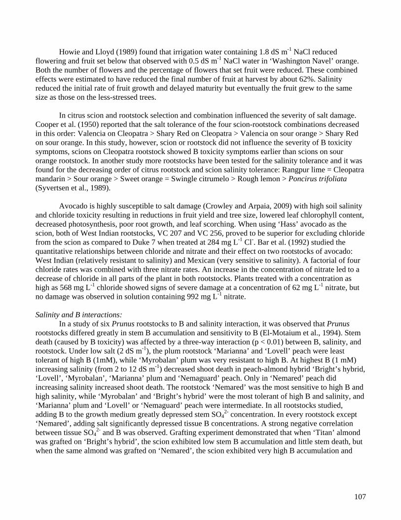
107

Howie and Lloyd (1989) found that irrigation water containing 1.8 dS m-1 NaCl reduced flowering and fruit set below that observed with 0.5 dS m-1 NaCl water in ‘Washington Navel’ orange. Both the number of flowers and the percentage of flowers that set fruit were reduced. These combined effects were estimated to have reduced the final number of fruit at harvest by about 62%. Salinity reduced the initial rate of fruit growth and delayed maturity but eventually the fruit grew to the same size as those on the less-stressed trees.

In citrus scion and rootstock selection and combination influenced the severity of salt damage.

Cooper et al. (1950) reported that the salt tolerance of the four scion-rootstock combinations decreased in this order: Valencia on Cleopatra > Shary Red on Cleopatra > Valencia on sour orange > Shary Red on sour orange. In this study, however, scion or rootstock did not influence the severity of B toxicity symptoms, scions on Cleopatra rootstock showed B toxicity symptoms earlier than scions on sour orange rootstock. In another study more rootstocks have been tested for the salinity tolerance and it was found for the decreasing order of citrus rootstock and scion salinity tolerance: Rangpur lime = Cleopatra mandarin > Sour orange > Sweet orange = Swingle citrumelo > Rough lemon > Poncirus trifoliata (Syvertsen et al., 1989).

Avocado is highly susceptible to salt damage (Crowley and Arpaia, 2009) with high soil salinity and chloride toxicity resulting in reductions in fruit yield and tree size, lowered leaf chlorophyll content, decreased photosynthesis, poor root growth, and leaf scorching. When using ‘Hass’ avocado as the scion, both of West Indian rootstocks, VC 207 and VC 256, proved to be superior for excluding chloride from the scion as compared to Duke 7 when treated at 284 mg L-1 Cl-. Bar et al. (1992) studied the quantitative relationships between chloride and nitrate and their effect on two rootstocks of avocado: West Indian (relatively resistant to salinity) and Mexican (very sensitive to salinity). A factorial of four chloride rates was combined with three nitrate rates. An increase in the concentration of nitrate led to a decrease of chloride in all parts of the plant in both rootstocks. Plants treated with a concentration as high as 568 mg L-1 chloride showed signs of severe damage at a concentration of 62 mg L-1 nitrate, but no damage was observed in solution containing 992 mg L-1 nitrate. Salinity and B interactions: In a study of six Prunus rootstocks to B and salinity interaction, it was observed that Prunus rootstocks differed greatly in stem B accumulation and sensitivity to B (El-Motaium et al., 1994). Stem death (caused by B toxicity) was affected by a three-way interaction (p < 0.01) between B, salinity, and rootstock. Under low salt (2 dS m-1), the plum rootstock ‘Marianna’ and ‘Lovell’ peach were least tolerant of high B (1mM), while ‘Myrobalan’ plum was very resistant to high B. At highest B (1 mM) increasing salinity (from 2 to 12 dS m-1) decreased shoot death in peach-almond hybrid ‘Bright’s hybrid, ‘Lovell’, ‘Myrobalan’, ‘Marianna’ plum and ‘Nemaguard’ peach. Only in ‘Nemared’ peach did increasing salinity increased shoot death. The rootstock ‘Nemared’ was the most sensitive to high B and high salinity, while ‘Myrobalan’ and ‘Bright’s hybrid’ were the most tolerant of high B and salinity, and ‘Marianna’ plum and ‘Lovell’ or ‘Nemaguard’ peach were intermediate. In all rootstocks studied, adding B to the growth medium greatly depressed stem SO4

2- concentration. In every rootstock except ‘Nemared’, adding salt significantly depressed tissue B concentrations. A strong negative correlation between tissue SO4

2- and B was observed. Grafting experiment demonstrated that when ‘Titan’ almond was grafted on ‘Bright’s hybrid’, the scion exhibited low stem B accumulation and little stem death, but when the same almond was grafted on ‘Nemared’, the scion exhibited very high B accumulation and

108

very high percentage stem death under high salt (12 dS m-1) in combination with high B (1 mM) treatments. In a sand tank study of ‘Kerman’ pistachio on three rootstocks with combined SO4

2- and Cl- salinity (3.5, 8.7, 12, or 16 dS m-1) and B (10 mg L-1) stress, Ferguson et al. (2002) demonstrated that all growth parameters (leaf area, trunk diameter and biomass) decreased as salinity increased, but were not significant until salinity exceeded 12 dS m-1. However, growth of ‘Kerman’ on P. atlantica and ‘UCB-1’ was considerably better than on P. integerrima at 16 dS m-1. The onset and severity of foliar injury differed among scions and treatments and was attributed primarily to B toxicity, rather than the effects of salinity. Concentrations of B in injured leaf tissue ranged from 1000 to 2500 ppm. Leaf injury decreased with increasing salinity, although leaf B was not significantly reduced suggesting an internal synergistic interaction between B and other mineral nutrients. However, for ‘Kerman’ on P. integerrima, the highest level of salinity produced the greatest injury, possibly as a combination of B plus Cl- and/or Na+ toxicity. References: Ashworth, Jr., LJ, Gaona SA, Surber E. 1985. Nutritional diseases of pistachio trees: potassium and

phosphorus deficiencies and chloride and boron toxicities. Phytopathology. 75: 1084-1091. Bar Y, Kafkafi U, Lahav E. 1992. Reducing chloride toxicity in avocado by nitrate.

http://www.avocadosource.com Beede RH, Brown PH, Kallsen C, Weinbaum SA. 2005. Diagnosing and correcting nutrient

deficiencies. In: Ferguson L (ed) Pistachio production manual. 4th edition. P. 147-157. Bernstein, L., J.W. Brown and H.E. Hayward. 1956. The influence of rootstock on growth and salt

accumulation in stone-fruit trees and almonds. Proc. Amer. Sot. Hort. Sci. 68:86-95. Brown PH, Hu H, Roberts WG. 1999. Occurrence of sugar alcohol determines boron toxicity symptoms

of ornamental species. J. Amer. Soc. Hort. Sci. 124: 347-352. Cooper WC, Cordell E. 1950. Salt and boron tolerance of Shary Red grapefruit and Valencia orange on

sour orange and Cleopatra mandarin rootstocks. Proc. Rio Grande Balley Hort. Inst. 4: 58-79. Crowley D, Arpaia M. 2009. Rootstock selections for improved salinity tolerance of avocado.

http://www.avocadosource.com Dhankhar DP, Dahiya SS. 1980. The effect of different levels of boron and soil salinity on the yield of

dry matter and its mineral composition in Ber (Zizyphus rotundifolia). Intl. Symp. Salt Affected Soils. Carnal pp. 396-403.

Eaton FM, Blair GY. 1935. Accumulation of boron by reciprocally grafted plants. Plant Physiology. 10: 411-424.

Ferguson L, Poss JA, Grattan SR, Grieve CM, Wang D, Wilson C, Donovan TJ, Chao C.-T. 2002. Pistachio rootstocks influence scion growth and ion relations under salinity and boron stress. J. Amer. Soc. Hort. Sce. 127: 194-199.

Grattan SR. 2002. Irrigation water salinity and crop production. University of California Agriculture and Natural Resources. Publication 8066. http://anrcatalog.ucdavis.edu.

Grattan SR, Grieve CM. 1999. Salinity mineral nutrient relations in horticultural crops. Scientia Horticulturae. 78: 127-157.

Gupta UC, Jame YW, Campbell CA, Leyshon AJ, Nicholaichuk W. 1985. Boron toxicity and deficiency: a review. Can J. Soil Sci. 65: 381-409.

Haas ARC. 1929. Toxic effect of boron on fruit trees. Bot. Gaze. 88: 113-131. Hall LW Jr., Killen WD, Anderson RD, Perry E. 2004. Analysis of historical salinity and boron surface

109

water monitoring data from the San Joaquin River watershed: 1985-2002. Environ. Monitoring and Assess. 95: 125-151.

Howie H, Lloyd J. 1989. Response of orchard ‘Washington Navel’ orange, Citrus sinensis (L) Osbeck to saline irrigation water. II Flowering, fruit set and fruit growth. Aust. J. Agric. Res. 40:371-380.

Kohl HC, Oertli JJ. 1961. Distribution of boron in leaves. Plant Physiology. 36: 420-424. Letey J. 2000. Soil salinity poses challenes for sustainable agriculture and wildlife. Calif. Agri. Future in

focus: 2000-2005. 54: 43-48. Maas EV. 1990. Crop salt tolerance. p. 262-304. In: K.K. Tanji (ed.). Agricultural salinity assessment

and management. ACSE Manuals and reports on Engineering Practice No. 71. Amer. Soc. Civil Eng. New York.

Maas EV. 1993. Salinity and citriculture. Tree physiology. 12: 195-216. Massai R, Remorini D, Tattini M. 2004. Gas exchange, water relations and osmotic adjustment in two

scion/rootstock combinations of Prunus under various salinity concentrations. Plant Soil. 259: 153-162.

Papadakis IE, Dimassi KN, Bosabalidis AM, Therios IN Patakas A, giannakoula A. 2004a. Effects of B excess on some physiological and anatomical parameters of ‘Navelina’ orange plants grafted on two rootstocks. Environ. And exp. Bot. 51: 247-257.

Papadakis IE, Dimassi KN, Bosabalidis AM, Therios IN, Patakas A, Ginnakoula A. 2004b. Boron toxicity in ‘Clementine’ mandarin plants grafted on two rootstocks. Plant Science 166: 539-547.

Rahmani A, Sardabi H, Daneshvar HA. 2006. Responses of cultivated and wild almonds to salinity. Acta Hort. 726, ISHS. 265-272.

Sanden B, Ferguson L, Kallsen C, Corwin D. 2007. Large-scale utilization of saline groundwater for development and irrigation of pistachios (P. integerrima) interplanted with cotton (G. barbadense). Acta Horticulturae. ISHS. 792:551-558.

Syvertsen JP, Boman B, Tucker DPH. 1989. Salinity in Florida citrus production. Proc. Fla. State Hort. Soc. 102: 61-64.

110

from Grattan SR (2002)

111

Salt Distributions and Salinity Management Under Drip Irrigation/Microirrigation

Blaine Hanson Department of Land, Air and Water Resources

University of California, Davis Drip irrigation has the potential of increased yield with less applied water. However, under saline conditions, adequate salinity control must occur to realize its potential. Drip irrigation has some specific advantages under saline conditions. First, no foliar absorption of salts occurs during irrigation. Second, the wetting pattern around emitters results in highly leached soil near the drip line, a zone where root density frequently is the highest, particularly for row crops. Third, high frequency drip irrigation can maintain relatively constant soil water content and soil salinity over time near drip lines. A main disadvantage of drip irrigation is salt accumulation near the periphery of the wetted pattern. Thus, the placement of emitters relative to the plant row is critical for crops that are sensitive to moderately sensitive to soil salinity. Salt accumulation above buried drip lines also is a concern. Salt Distribution Around Drip Lines Factors affecting root zone soil salinity under drip irrigation include the salinity of the irrigation water, amount of applied water, soil hydraulic characteristics, placement of drip lines relative to plant rows, subsurface vs. surface drip lines, and under saline, shallow ground water conditions, the ground water depth and salinity. The salt pattern will reflect the water flow patterns under drip irrigation. Near the emitter, soil salinity will approach the salinity of the irrigation water. Soil salinity increases slightly with radial distance from the emitter until near the periphery of the wetted pattern where large increases in salinity occur over small increases in radial distance. Salt leaching occurs near the drip line, whereas salt accumulates near the periphery of the wetted pattern. Under conditions of continued high frequency irrigation (multiple irrigations per week) over time in commercial fields, considerable leaching can occur beneath drip lines. Low salinity levels occurred near the drip lines and extended downward with salt accumulating between drip lines and near the edge of the bed in a sandy loam soil (fig. 1). Under subsurface drip irrigation, salt accumulated above the drip line with the highest levels near the soil surface indicating no leaching above the drip line. Leaching occurred below the drip line as indicated by the relatively low salinity levels near and extending below the drip line (fig. 2). Under saline, shallow ground water conditions, a relatively uniform soil salinity profile was found for a water table depth of about 6 ft (fig. 3A) for an irrigation water of EC of 0.3 dS/m-1. For a water table depth of about 3 ft, soil salinity varied spatially around the drip line (fig. 3B). Higher soil salinity near the drip line occurs for higher irrigation water salinity (not shown). Salinity Control under Drip Irrigation The key to profitable drip irrigation under saline conditions is adequate salinity control in the root zone. Salinity control involves leaching salts from the root zone by applying irrigation water in excess of the

112

soil moisture depletion. The leaching fraction, used as a measure of adequacy of leaching, is the ratio of the amount of water draining below the root zone to the amount of infiltrated water. Leaching under drip irrigation depends on the EC of the irrigation water, the amount of water applied, and the wetting pattern, which is also dependent on the applied amount and soil hydraulic characteristics. No leaching around the drip line due to insufficient applied water can cause a zone of high soil salinity near drip lines (fig. 4A), whereas a low salt zone occurs around drip lines under leaching conditions (fig. 4B). Increasing the applied water increases the leaching fraction, which results in more low salt soil around drip lines (not shown). Research has shown that as the low-salt zone increases, yield increases because of an increase in crop evapotranspiration due to a combination of lower soil salinity near the drip line, a larger zone of low salt soil around drip lines, and higher soil water contents near the drip line as the leaching fraction increases. Estimating Leaching Fractions Several methods have been historically used to determine leaching fractions in commercial fields. One method requires measurements of the irrigation water electrical conductivity (EC) and the average root zone soil salinity (ECe). Chloride concentrations are sometimes used instead of the EC. These data are then related to the leaching fraction using leaching curves or appropriate equations. However, both salt patterns and root patterns vary spatially around drip lines, which can introduce uncertainty in estimating leaching fractions using soil salinity data. The water balance is commonly used to estimate field wide leaching fractions using cumulative amounts of applied water and evapotranspiration for a given time period. The leaching amount is the difference between applied water and evapotranspiration. However, field studies indicate that the water balance method of estimating leaching fractions may be inappropriate under drip/microsprinker irrigation because it does not account for the effect of spatially-varying soil water patterns of drip irrigation/microirrigation which cause leaching below the drip lines, even for conditions considered to be deficit irrigation, i.e. applied water amounts are smaller than the 100% evapotranspiration. A USDA/ARS study estimated actual leaching fractions for drip-irrigated almonds in silt loam to clay loam soil using soil chloride concentrations. Amounts of applied irrigation water were 50%, 100%, and 150% of the evapotranspiration of the 100% water application. The water balance method indicated that no leaching occurred for the 50% and 100% applied water treatments and a 50% leaching fraction for the 150% treatment, but actual leaching fractions, calculated from chloride concentrations, were 4 to 6% for the 50% water treatment, 10 to 22% for the 100% treatment, and 31 to 36% for the 150% treatment. These values were based on the soil chloride levels of the first 3 to 5 feet from the tree at the bottom of the root zone.

A UC Davis study showed that under saline shallow ground water conditions, the field-wide leaching amounts calculated using the water balance approach revealed little or no field-wide leaching in four commercial fields of processing tomatoes, which suggested inadequate salinity control and raised questions about the long-term viability of drip irrigation under saline conditions. The soil salinity data, however, clearly showed substantial localized leaching around the drip lines and that the leaching was concentrated near the drip lines. Computer simulations revealed actual or localized leaching fractions of 7.7% (60% water application) to 30.5% (115% water application) and 24.5% for the 100% water

113

application. Even for applications considered to be severe deficit irrigation, drainage below the root zone occurred, caused by the wetting patterns under drip irrigation. Under subsurface drip irrigation, no leaching by drip irrigation occurs above the drip lines. Thus, periodic leaching either by rainfall or sprinkle irrigation is necessary to control root zone soil salinity above the drip lines. Sufficient leaching water should be applied to move the salts below the drip line, where they will eventually be leached by subsequent drip irrigation. The placement of drip lines relative to plant rows is critical in salinity control with drip irrigation, particularly for row crops. Salinity control will be best where drip lines and plant rows coincide because the root density of row crops generally will be the highest near the drip lines, where leaching will be the greatest. This may not be the case for tree/vine crops. Offsetting drip lines from plant rows can shift the zone of high root density away from the zone of highly leached soil, and in some cases, into the zone of salt accumulation. Considerations

• Seasonal water applications should be at least equal to the seasonal evapotranspiration. This amount of water provides sufficient localized leaching, and under conditions of saline shallow ground water, minimizes crop water use of the ground water, and prevents ground water intrusion into the root zone.

• The electrical conductivity of the low-salt soil around drip lines will reflect the electrical conductivity of the irrigation water. The effect of the irrigation water salinity on crop yield will depend on the crop’s sensitivity to yield, the salinity of the irrigation water, and the amount of leaching.

• Periodic leaching of salt accumulated above the buried drip lines will be necessary with sprinkle irrigation for stand establishment if winter and spring rainfall is insufficient.

• Drip irrigation systems should be designed for a high uniformity of applied water.

• Drip irrigation systems should be properly maintained to prevent emitter clogging.

114

ECe

Figure 1. Salt pattern under surface drip irrigation with two drip lines. Units of scale are dS/m.

Figure 2. Salinity pattern for subsurface drip line. Salinity units are dS/m.

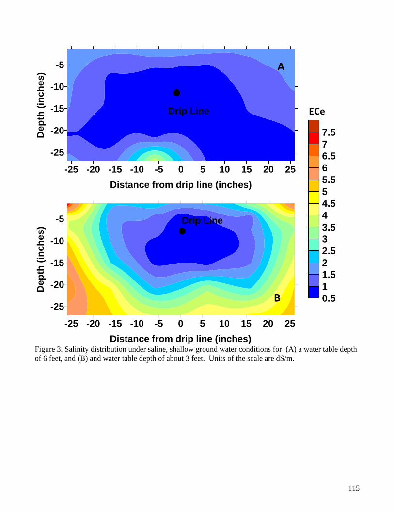
115

-25 -20 -15 -10 -5 0 5 10 15 20 25Distance from drip line (inches)

-25

-20

-15

-10

-5

Dep

th (i

nche

s)

Drip Line

A

0.511.522.533.544.555.566.577.5

ECe

-25 -20 -15 -10 -5 0 5 10 15 20 25Distance from drip line (inches)

-25

-20

-15

-10

-5

Dep

th (i

nche

s)

Drip Line

B

Figure 3. Salinity distribution under saline, shallow ground water conditions for (A) a water table depth of 6 feet, and (B) and water table depth of about 3 feet. Units of the scale are dS/m.

116

4 6 8 10 12 14 16 18-10

-8

-6

-4

-2

0.00.51.01.52.02.53.03.54.04.55.05.56.0

April

Drip Line

4 6 8 10 12 14 16 18 20 22Distance Across Bed (inches)

-12

-10

-8

-6

-4

-2

July

Dep

th (i

nche

s)

Drip Line

ECe

A

B

Figure 4. Salinity distribution for a (A) no leaching condition and (B) leaching condition. Units of the scale are dS/m.

117

Drip Irrigation Filtration and Water Treatment to Prevent Clogging

Larry Schwankl, UC Cooperative Extension UC Davis & UC Kearney Ag Center 559-646-6569 schwankl@uckac.edu

FILTRATION

Introduction

Filtration of water to remove particulate matter and biological contaminants is critical to the efficient operation of many pressurized irrigation systems, but it is particularly important for microirrigation systems. Drip and microsprinkler systems may use screen, disk, or sand media filters to remove small particulates and organic contaminants to prevent clogging. The choice of which filter to use is often based on the water quality. Filtration Requirements

The degree of filtration recommended for specific drip emitters and microsprinklers is available from the manufacturer and should be followed. The level of filtration is based primarily on the emitter flow pathway size. Filtration removes particles significantly smaller than the flow path size since smaller particles can “bridge”, often in conjunction with biological or chemical precipitate problems, and cause clogging. The degree of filtration of screen and disk filters is designated by the mesh size. The mesh size is the number of openings per inch of screen. The degree of filtration of sand media filters is determined by the size of the sand media particles with the sand media sizes referenced to equivalent mesh size (Table 1).

Table 1. Sand media size and screen mesh designation

Sand no. Effective sand size (in.)

Screen mesh designation

8 0.059 70 11 0.031 140 16 0.026 170 20 0.018 230 30 0.011 400

Mineral particulates in irrigation water range in size from sands to silts to clays. The equivalent mesh sizes for these mineral particles are given in Table 2. Few microirrigation systems require greater than 200-mesh filtration. Note that small sand particles, silts, and clays will pass through a 200-mesh screen. These very small particles can pass though drip emitters or microsprinklers, or they may settle out in the pipelines or lateral lines requiring flushing to be removed (discussed later).

118

Table 2. Particle size classification by mesh size.

Particle Size Mesh equivalent

Very coarse sand 10-180 mesh Coarse sand 18-35 mesh

Medium sand 35-60 mesh Fine sand 60-160 mesh

Very fine sand 160-270 mesh Silt 270-400 mesh Clay Smaller than 400 mesh

Types of Filters

Suction Screen Filters

Suction screens are used on centrifugal pump intakes where there is a significant problem with large particulates and trash in the water as can be the case from surface water sources such as rivers and streams. Used by themselves, they may provide adequate filtration for sprinkler irrigation systems, but not for microirrigation systems. Rather, they may be the first filtration step for microirrigation systems, removing the large particulates which would quickly overwhelm the screen, disk, or media filters also being used. To be effective, suction screen filters should filter out the contaminants and keep themselves clean. Some suction screen filters continually rotate and use water jets to clean the contaminants off the screen. The water flowing by the intake screen carries the contaminants downstream. Centrifugal Sand Separators

Centrifugal sand separators are well suited to removing larger sand particles which may be present in both surface water sources and in groundwater. They are designed to “swirl” the water passing through them, using centrifugal forces to remove the sand particles. Larger sand particles must be removed from microirrigation systems since they will cause clogging. While screen, disk, or sand media filters can all remove sand particles, large volumes of sand may clog these filters quickly. In microirrigation systems, centrifugal sand separators are often used as the first stage filtration method, followed by screen, disk, or sand media filters. Screen Filters

Two types of screen filters are common – pressurized screen filters and gravity flow screen filters. In a gravity flow screen filter, water is allowed to run over the screen filter, open to the atmosphere, with the filtered water falling through the screen and being collected. The contaminants caught on the screen are either washed off the screen by the water flowing across the steeply inclined screen, or, in another design a slightly-inclined screen is continually washed clean by a rotating jet which moves the contaminants into a collection trough. Use of a gravity screen filter requires the irrigation water to be pressurized following filtration. A pressurized screen filter is plumbed into the irrigation system and filtration is accomplished as the pressurized water passes through it. Screen filters are widely used in microirrigation systems, particularly where groundwater is used. Pressurized screen filters may not be appropriate for use with

119

water high in organic matter. The organic contaminants can quickly clog the screen and be difficult to remove. Once the screen is clogged, there may be a significant pressure loss across the screen and the flow rate through the screen may be substantially reduced. Installation of pressurized screen filters with upstream and downstream pressure gauges is recommended so that the manager can easily note when the screen needs cleaning. Some pressurized screen filters require the screen element to be manually removed for cleaning. Others have a backwash system so that the screens can be cleaned without disassembling the filter. Some of these backwash systems are operated manually while others allow the backwash to be done automatically, either on a set time interval and/or on a pressure loss across the screen, sensing system. The recommended, maximum flow rate through the screen filter will be specified by its manufacturer. Waters high in contaminants will clog the filter more quickly. Automatic backwash filters may be advantageous under these conditions, or an alternative would be a larger filter element (or more filters plumbed in parallel) to increase the interval between manual cleanings. Disk Filters

Disk filters consist of a stack of thin disks, tightly held together, each having a series of very small grooves along their sides. Water is filtered as it flows through the grooves. The degree of filtration is measured as mesh size. Disk filters effectively filter particulate matter and they will remove organic contaminants from the water but the organic contaminants tend to clog the disk filter quickly, necessitating frequent cleaning. Most disk filters must be disassembled and cleaned manually, but there are automatic backwash disk filters available. Where the water is high in organic matter, a disk filter with an automatic backwash system may be advantageous. The water required for backwashing disk filters is less than that for sand media filters.

Sand Media Filters

Sand media filters are tanks made of epoxy-coated metal or stainless steel. They are filled with a filtering media, often silica sand. The particle size of the media is selected according to the desired degree of filtration (Table 1). Water contaminants are filtered from the water as the water flows down through the media. An under-drain, made from either an epoxy cake or perforated pipe at the bottom of the tank, collects the filtered water and retains the filtering media during filtration. Sand media filters have a greater filtering capacity than screen or disk filters and can be used to remove both organic contaminants and particulate matter, making them well suited for filtering surface waters. At least two media filter tanks, plumbed in parallel, are required at a site so that as one filter is being backwashed, the other filter(s) can continue to provide water for the backwashing and for irrigation. Additional sand media filter tanks can be added if increased filtration capacity is needed. Frequently, a backup screen filter is placed downstream of the sand media filters to catch any sand escaping the media filters, either from routine operation or from failure of the media filter’s under-drain system. The recommended flow rate for sand media filters is 15 to 25 gallons per minute per square foot (35 to 60 cubic meters per hour per square meter) of filter surface area. Manufacturers of sand media filters provide recommended filter flow rates both for filtration and for backwashing of filters. These recommendations should be followed. Backwashing of sand media filters can either be done manually or automatically. When backwashing, a three-way valve at the top of the filter changes position and clean water passes upward from the under-drain system. This suspends and agitates the filter media with contaminants being

120

flushed out of the filter with the backwash water. Pressure gauges should be installed upstream and downstream of the filters and backwashing should be done when the pressure drop across the filters (approximately 5 psi) indicates that they are dirty. Automatic backwashing systems allow the media filters to be cleaned on a desired time interval or when the pressure drop across the filter exceeds a selected value. Disposal of backwash water can be a problem when using sand media filters. The backwash flow rate is nearly 200 gallons per minute (45 cubic meters per hour) for a typical 48-inch (1.2 meter) sand media filter, so a substantial volume of backwash water is generated. Some microirrigation system managers are even constrained to disposing of backwash water using reservoirs or tile drain systems. Microirrigation System Flushing

Small sand, silt, and clay particles pass through the filters used in microirrigation systems. These fine particles frequently settle in the pipelines and polyethylene lateral lines of microirrigation systems and, unless they are flushed out, can lead to clogging of drip emitters or microsprinklers. Appropriately sized flush-out valves should be located on the end of pipelines. These valves can be opened and the particles which have settled in the pipelines flushed out. Following flushing of the pipelines, the ends of the lateral lines should be opened, a few at a time, and allowed to flush clear. In drip irrigation systems designed for row crops, the lateral lines may be manifolded together to allow more convenient flushing. An alternative to manual flushing of lateral lines is to use self-flushing end caps on the lateral lines. These end caps allow a short flush at the beginning and end of the irrigation event. CHEMICAL TREATMENT

Chemical treatment of water for microirrigation systems is required when the water may cause chemical precipitate or biological clogging of the microirrigation drippers or microsprinklers. The chemical treatment varies depending on the clogging source. Biological Clogging

Biological clogging problems are most often associated with surface waters—waters that have been stored in reservoirs or ponds, or transported in canals, rivers, etc. While it is often difficult to identify the biological contaminant, algae and biological slimes are often major contributors to biological clogging. Groundwaters high in iron may also be a biological clogging hazard for microirrigation systems. The dissolved iron in the water provides an energy source for the iron bacteria. The gelatinous slime produced by the iron bacteria can clog emitters, often in conjunction with particulates (silt or clay particles, chemical precipitates, or other contaminants) for which they can provide a “glue” to bind particles together. Levels of Concern

Certainly any waters that appear “green” prior to use are capable of causing biological clogging but even surface waters which appear clean may be a clogging hazard. Since surface water quality can change drastically across the season, often caused by rising temperatures and falling water levels, it is often not worthwhile to attempt to quantify the biological clogging hazard. It is better to monitor the

121

microirrigation system for any sign of biological clogging and if it appears, treat the water. Often there is a history of biological clogging problems and the manager knows that treatment is required. Treatment

Biological treatment methods involve using a biocide that kills the biological contaminant. The two most common biocides used with microirrigation systems are chlorine and copper. Historically, chlorine products have been most frequently injected into microirrigation systems while copper products have been used to control biological growth in ponds and reservoirs. This has changed somewhat with the availability of new copper-based formulations developed for injection into microirrigation systems. The following are recommended levels of chlorine for biological contaminant control.

Injection Method Chlorine concentration at the end of the last lateral

Continuous injection 1-2 ppm

Periodic injection 10-20 ppm Contact time between the water with chlorine and biological contaminant is important. Periodic chlorine injections should be at least 4 hours and longer is better. Chlorine injections can continue up to system shutdown, with the chlorinated water left sitting in the lines. This may have limited effect on above-ground lines since they tend to drain out at the lowest point(s), but it may help clean up other pats of the system. Copper levels to provide effective biocide protection are also quite low, often copper levels less than 5 pm are effective. Follow manufacturer’s recommendation for formulations containing copper. Chemical Precipitate Clogging

Most chemical precipitate clogging problems are associated with groundwater sources. Elements in solution in the groundwater may precipitate above ground and if the precipitates may clog the microirrigation system’s small emitter passageways. There are many potential chemical precipitates which can cause clogging problems, but calcium carbonate (line) and iron are two of the more common problems. Lime precipitation is the most common and can occur when calcium and bicarbonate levels in the water are 2 meq/l or higher and the water pH is 7.5 or higher. The most common treatment for lime precipitation clogging is to lower water pH to 7.0 or below. A pH in the range of 6 to 6.5 is effective in removing the calcium carbonate precipitate while not being of risk to system components. Iron precipitate clogging is not as common as lime precipitation but it is more difficult to deal with. Iron precipitate clogging can occur when the iron levels are 0.2 ppm or higher although most problems occur when iron levels are 1 ppm or higher. Water pH only needs to be 4.0 or higher fro iron precipitation so this pH level includes nearly all waters. Most people deal with iron precipitation problems by pumping the groundwater into a pond or reservoir where the iron precipitates and settles out. Adequate time is needed for the small precipitates to settle. This dictates an adequately sized pond.

122

A relatively new way of dealing with iron and calcium carbonate precipitation problems is to continually inject a product containing phosphonate or phosphonic acid. The phosphonate (or phosphonic acid), injected at rates of 5 ppm or less, interfere with the precipitation. There are a number of anti-clogging formulations on the market which contain phosphonate or phosphonic acid as their active ingredient. Particularly for iron clogging problems, for which only aeration/precipitation and settling is the solution, the phosphonate or phosphonic acid products may be very beneficial.

123

Impacts of conservation tillage and cover cropping on productivity, profitability and soil properties in a San Joaquin Valley cotton / tomato production system

J.P. Mitchell1, W.R. Horwath2, R.J. Southard2, K.M. Klonsky3, , D.S. Munk4,

A.Shrestha5, T. Gohlke6, R. Bickel7, John Diener8, and Scott Schmidt9

1Department of Plant Sciences, University of California, Davis, 95616 mitchell@uckac.edu, , 2Department of Land, Air and Water Resources, University of California, Davis, 95616

wrhorwath@ucdavis.edu and rjsouthard@ucdavis.edu, 3Department of Agricultural and Natural Resource Economics, University of California, 95616 klonsky@primal.ucdavis.edu, 4Cooperative

Extension Fresno County, Fresno, CA 93702 dsmunk@ucdavis.edu, 5Department of Plant Science, California State University, Fresno, 93740 ashrestha@csufresno.edu, 6USDA Natural Resources

Conservation Service, West National Technology Support Center, Portland, OR 97232 tom.gohlke@por.usda.gov, 7USDA natural Resources Conservation Service, Davis, CA 95616

rita.bickel@ca.usda.gov, 8 Red Rock Ranch, Five Points, CA 93262 john@rrrinc.net, and 9Farming ‘D’, Five Points, CA 93624 sschmidt4@att.net

Abstract To determine their long-term impacts on productivity, profitability and soil properties, we evaluated standard (ST) and conservation (CT) tillage systems for a cotton / tomato rotation with (CC) and without (NO) winter cover crops in a Panoche clay loam (fine-loamy, mixed, superactive, Thermic Typic Haplocambids) soil in Five Points, CA from 1999 - 2007. In this study, the number of tractor trips across the field was reduced by about 50% for tomato and 40% for cotton in the CT systems relative to the ST approaches. Following the establishment of the tillage and cover crop treatments, tomato yields in the CTNO system were generally similar to or higher than yields in the STNO system. CT cotton yields were lower than ST yields in the first four years of the study, but similar in subsequent years. Rainfed cover crop biomass averaged about 3500 lbs throughout the study. After eight years, soil carbon was highest in the CTCC system and lowest in the STNO system. Mean Soil Conditioning Index values were 0.43 for the CTNO and 0.52 for the CTCC, and -0.71 and -0.96 for the STNO and STCC systems, respectively. Estimates of fuel use in the CT systems were 28% of those of the ST systems.

Introduction Lack of familiarity with conservation tillage (CT) practices for row crops such as tomatoes and cotton in California’s San Joaquin Valley (SJV) as well as uncertainties associated with managing risks when major changes in tillage operations are implemented have resulted in very little acreage of these crops currently being farmed using CT (Mitchell et al., 2009) In recent years, however, increased production costs and interest in reducing labor needs in SJV crop production systems have provided incentives for CT options, though adoption of these systems remains quite low (Conservation Tillage and Cropping Systems Workgroup, 2009). In 1999, we began research in Five Points, CA to evaluate conservation tillage tomato and cotton systems with and without winter cover crops in terms of productivity, costs, and soil carbon. Following the first four years of this study, no increases were seen in total soil carbon in the surface 0 – 30 cm of

124

soil, however a redistribution of both carbon and nitrogen was seen from deeper soil into the top 5 cm of soil under CT compared with traditional tillage (Veenstra et al., 2006). Similar to other long-term studies with cover cropping (Horwath et al., 2002), a significant increase in soil carbon and nitrogen was seen in the 0 – 30 cm layer (Veenstra et al., 2006). We report here aspects of how the tillage and cover crop systems performed after eight years of the study.

Materials and Methods A field comparison of conservation and standard tillage cotton and tomato rotations with and without winter cover crops was established in the fall of 1999 at the University of California West Side Research and Extension Center in Five Points, CA. The field was divided into two halves; a tomato (Lycopersicon esculentum)-cotton (Gossypium hirsutum L.) rotation was used in one half, and a cotton-tomato rotation was pursued in the other half to allow tomato and cotton plantings and experiments to occur within each year. Management treatments of standard tillage without cover crop (STNO), standard tillage with cover crop (STCC), conservation tillage without cover crop (CTNO), and conservation tillage with cover crop (CTCC) were replicated four times in a randomized complete block design on each half of the field. Treatment plots consisted of six beds, each measuring 9.1 x 82.3 m. Six-bed buffer areas separated tillage treatments to enable the different tractor operations that were used in each system. A cover crop mix of Juan triticale (Triticosecale Wittm.), Merced ryegrain (Secale cereale L.) and common vetch (Vicia sativa) was planted at a rate of 89.2 kg ha-1 (30% triticale, 30% ryegrain and 40% vetch by weight) in late October in the standard and conservation tillage plus cover crop plots and irrigated once in 1999. In each of the subsequent years, no irrigation was applied to the cover crops, which were planted in advance of any early winter rains. The cover crops were chopped in mid-March of the following years using a Buffalo Rolling Stalk Chopper (Fleischer, NE). In the STCC system, the chopped cover crop was disked into the soil to a depth of about eight inches and 1.52 m-wide beds were reformed prior to tomato transplanting. The chopped cover crop in the CTCC was sprayed with a 2% solution of glyphosate after chopping and left on the surface as a mulch. Conventional intercrop tillage practices that knock down and establish new beds following harvest were used in the standard tillage (ST) systems (Table 1). The conservation tillage systems were managed from the general principle of trying to reduce primary, intercrop tillage to the greatest extent possible. Zone production practices that restrict tractor traffic to furrows were used in the CT systems, and planting beds were not moved or destroyed in these systems during the entire four years. Table 1. Comparison of standard tillage (ST) and conservation tillage (CT) system operations with and without cover crops used in this study for tomato. (Each “X” indicates a separate instance of each operation) With cover crop Without cover crop Operation ST CT ST CT Shred cotton X X Undercut Cotton X X Disc XXXX XX Chisel X X Level (Triplane) X X List beds XX X

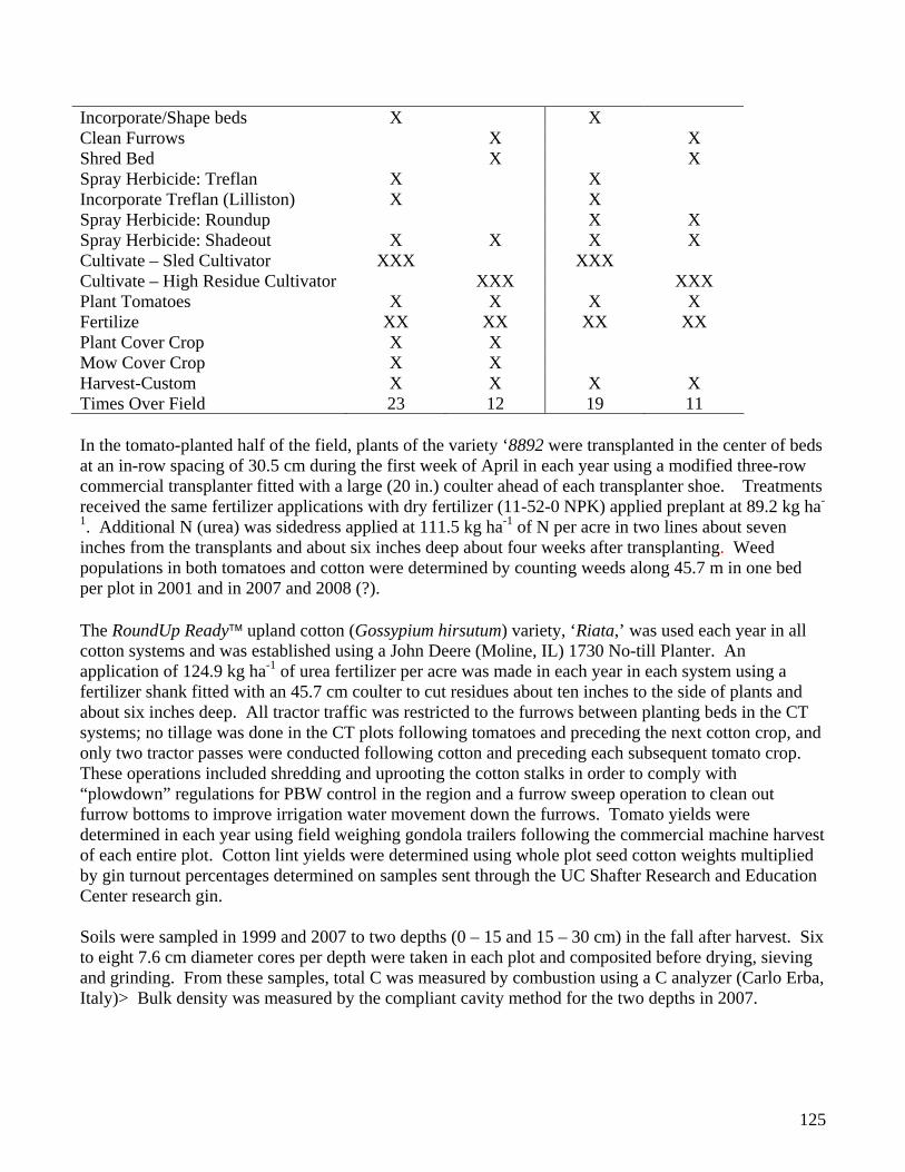
125

Incorporate/Shape beds X X Clean Furrows X X Shred Bed X X Spray Herbicide: Treflan X X Incorporate Treflan (Lilliston) X X Spray Herbicide: Roundup X X Spray Herbicide: Shadeout X X X X Cultivate – Sled Cultivator XXX XXX Cultivate – High Residue Cultivator XXX XXX Plant Tomatoes X X X X Fertilize XX XX XX XX Plant Cover Crop X X Mow Cover Crop X X Harvest-Custom X X X X Times Over Field 23 12 19 11 In the tomato-planted half of the field, plants of the variety ‘8892 were transplanted in the center of beds at an in-row spacing of 30.5 cm during the first week of April in each year using a modified three-row commercial transplanter fitted with a large (20 in.) coulter ahead of each transplanter shoe. Treatments received the same fertilizer applications with dry fertilizer (11-52-0 NPK) applied preplant at 89.2 kg ha-

1. Additional N (urea) was sidedress applied at 111.5 kg ha-1 of N per acre in two lines about seven inches from the transplants and about six inches deep about four weeks after transplanting. Weed populations in both tomatoes and cotton were determined by counting weeds along 45.7 m in one bed per plot in 2001 and in 2007 and 2008 (?). The RoundUp Ready™ upland cotton (Gossypium hirsutum) variety, ‘Riata,’ was used each year in all cotton systems and was established using a John Deere (Moline, IL) 1730 No-till Planter. An application of 124.9 kg ha-1 of urea fertilizer per acre was made in each year in each system using a fertilizer shank fitted with an 45.7 cm coulter to cut residues about ten inches to the side of plants and about six inches deep. All tractor traffic was restricted to the furrows between planting beds in the CT systems; no tillage was done in the CT plots following tomatoes and preceding the next cotton crop, and only two tractor passes were conducted following cotton and preceding each subsequent tomato crop. These operations included shredding and uprooting the cotton stalks in order to comply with “plowdown” regulations for PBW control in the region and a furrow sweep operation to clean out furrow bottoms to improve irrigation water movement down the furrows. Tomato yields were determined in each year using field weighing gondola trailers following the commercial machine harvest of each entire plot. Cotton lint yields were determined using whole plot seed cotton weights multiplied by gin turnout percentages determined on samples sent through the UC Shafter Research and Education Center research gin. Soils were sampled in 1999 and 2007 to two depths (0 – 15 and 15 – 30 cm) in the fall after harvest. Six to eight 7.6 cm diameter cores per depth were taken in each plot and composited before drying, sieving and grinding. From these samples, total C was measured by combustion using a C analyzer (Carlo Erba, Italy)> Bulk density was measured by the compliant cavity method for the two depths in 2007.

126

A calendar of operations was maintained for each of the systems and the equipment used and materials applied were recorded. The cost of each operation for each system was estimated using a model of a hypothetical farm under each of the four systems. The time required for each operation, fuel, lube, and repairs was generated using agricultural engineering equations. The input costs for seed, transplants, fertilizer and pesticides was obtained from local input suppliers and entered into the model. The cost of production and resource use for each of the systems were then compared. In particular, the model summarizes the labor requirements for both tractor operators and irrigation labor as well as fuel use. Finally, the yield data were used to calculate the expected gross returns using local market information. From this, the economic feasibility of each system was estimated and the relative profitability determined. Input and operations data were also used to estimate soil loss using the Revised Universal Soil Loss Equation (RUSLE) 2, to compute the soil condition index (SCI) and the soil tillage intensity index (STIR), and to estimate fuel use of each tillage / cover crop management system. The SCI and STIR are predictive soil management index tools that are required in several USDA Natural Resource Conservation Service (NRCS) criteria of practice standards that are used in assessing applications for Environmental Quality Incentives (EQIP) and Conservation Security (CSP) Programs of the Farm Security and Rural Investment Act of 2002 (Zobeck et al., 2007).

Results and Discussion Cover crop biomass Amounts of cover crop biomass produced during the study varied widely and closely corresponded to rainfall (Table 2). In 1999 – 2000, the cover crop was sprinkle-irrigated in order to establish the experimental treatments, however, in each of the following years, cover crop establishment and growth depended on winter rain. Cover crop biomass production over the 1999 – 2008 period averaged about 3,427 lbs of dry matter per acre. Table 2. Cover crop biomass in STCC and CTCC systems, 2000 – 2007 South 2000 2001 2002 2003 2004 2005 2006 2007 (lbs/ac) (lbs/ac) (lbs/ac) (lbs/ac) (lbs/ac) (lbs/ac) (lbs/ac) (lbs/ac) STCC 8036 3604 1226 2281 1732 6661 1461 28 CTCC 8344 2798 1895 5063 1744 8327 1282 66 North STCC 7850 4058 3121 2031 2449 5223 3320 10 CTCC 7889 3966 4236 3919 3192 5677 3169 58

Tomato and cotton productivity When averaged over the 2001 – 2008 period when the tillage system comparisons had been established, tomato yields were higher in the two systems without cover crops than in the CC systems, higher for the CT systems compared to the ST systems, and comparable to typical yields in Fresno County during these years. A significant cover crop X tillage system interaction that indicated higher yields in the CTCC than in the STCC systems. There was no year X cover crop X tillage system; the STNO, STCC< CTNO and CTCC effects on tomato yields were consistent year after year.

127

Higher tomato yields in the NO systems relative to the CC systems may have resulted form greater difficulties we experienced in transplanting tomatoes into the generally higher surface residue conditions of the CC systems and also the possibility of soil nitrogen immobilization in the CC systems which were predominantly composed of more triticale and rye relative to the legume, vetch. Cotton yields were generally higher in the ST systems during the first four years of the study, but there were no significant differences during later years. Soil conditioning index The SCI has been proposed by NRCS as a predictor of the consequences of management actions on soil organic carbon, but has recently been shown to be more closely associated with a more labile form of soil organic carbon known as particulate organic matter, or POM-C, as well as what have been termed the residue equivalent value (REV) that drives organic matter accumulation in the soil. The NRCS currently uses the SCI as one of its criteria for determining eligibility for Farm Bill conservation programs such as EQIP and CSP (Zobeck et al., 2007) The computed SCI values in Table 3 seem to be closely associated with the field operations that were used in the farm tillage and cover crop systems. SCI values were negative for the two ST systems and positive for the CT systems. Table 3. Tillage and cover crop system erosion estimates, soil condition index sub-factors, soil

tillage intensity rating and estimates of diesel fuel use. Croppin

g System*

Erosion Estimates‡ Soil conditioning index factors§

STIR (Averag

e Annual)

Diesel fuel use

Fuel cost for entire simulation

WEPS RUSLE2

OM FO ER SCI ($)

(Mg ha-

1) (Mg ha-

1)

STNO 2.1 0.2 -0.19 -1.6 0.01

1 -0.71 261 32 128.6

STCC 1.0 0.07 0.20 -2.9 0.53 -0.96 390 40 160.6 CTNO 0 0.04 -0.11 0.70 0.98 0.43 30.6 9.3 36.8 CTCC 0 0.03 0.18 0.63 0.99 0.52 37.1 11 43.27 * STNO = Standard tillage no cover crop, STCC = Standard tillage with cover crop, CTNO = Conservation tillage no cover cro CTCC = Conservation tillage with cover crop ‡ WEPS = wind erosion; RUSLE2 -= revised universal soil loss equation § SCI = soil conditioning index value; OM = SCI organic matter sub-factor; FO = SCI field operations subfactor; ER = SCI erosion subfactor; STIP = SCI soil tillage intensity rating

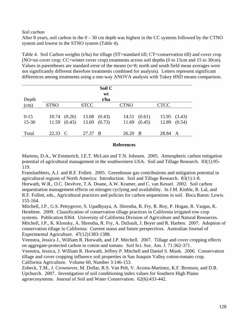
128

Soil carbon After 8 years, soil carbon in the 0 – 30 cm depth was highest in the CC systems followed by the CTNO system and lowest in the STNO system (Table 4). Table 4. Soil Carbon weights (t/ha) for tillage (ST=standard till; CT=conservation till) and cover crop (NO=no cover crop; CC=winter cover crop) treatments across soil depths (0 to 15cm and 15 to 30cm). Values in parentheses are standard error of the means (n=8; north and south field mean averages were not significantly different therefore treatments combined for analysis). Letters represent significant differences among treatments using a one-way ANOVA analysis with Tukey HSD means comparison.

Soil C

wt Depth t/ha (cm) STNO STCC CTNO CTCC 0-15 10.74 (0.26) 13.68 (0.43) 14.51 (0.61) 15.95 (3.43) 15-30 11.59 (0.43) 13.69 (0.73) 11.69 (0.45) 12.89 (0.54) Total 22.33 C 27.37 B 26.20 B 28.84 A

References

Martens, D.A., W.Emmerich, J.E.T. McLain and T.N. Johnsen. 2005. Atmospheric carbon mitigation potential of agricultural management in the southwestern USA. Soil and Tillage Research. 83(1):95-119. Fransluebbers, A.J. and R.F. Follett. 2005. Greenhouse gas contributions and mitigation potential in agricultural regions of North America: Introduction. Soil and Tillage Research. 83(1):1-8. Horwath, W.R., O.C. Devêvre, T.A. Doane, A.W. Kramer, and C. van Kessel. 2002. Soil carbon sequestration management effects on nitrogen cyclying and availability. In J.M. Kinble, R. Lal, and R.F. Follett, eds., Agricultural practices and policies for carbon sequestions in soil. Boca Raton: Lewis. 155-164. Mitchell, J.P., G.S. Pettygrove, S. Upadhyaya, A. Shrestha, R. Fry, R. Roy, P. Hogan, R. Vargas, K. Hembree. 2009. Classification of conservation tillage practices in California irrigated row crop systems. Publication 8364. University of California Division of Agriculture and Natural Resources. Mitchell, J.P., K. Klonsky, A. Shrestha, R. Fry, A. DuSault, J. Beyer and R. Harben. 2007. Adoption of conservation tillage in California: Current status and future perspectives. Australian Journal of Experimental Agriculture. 47(12)1383-1388. Veenstra, Jessica J., William R. Horwath, and J.P. Mitchell. 2007. Tillage and cover cropping effects on aggregate-protected carbon in cotton and tomato. Soil Sci. Soc. Am. J. 71:362-371. Veenstra, Jessica, J. William R. Horwath, Jeffrey P. Mitchell and Daniel S. Munk. 2006. Conservation tillage and cover cropping influence soil properties in San Joaquin Valley cotton-tomato crop. California Agriculture. Volume 60, Number 3:146-153. Zobeck, T.M., J. Crownover, M. Dollar, R.S. Van Pelt, V. Acosta-Martinez, K.F. Bronson, and D.R. Upchurch. 2007. Investigation of soil conditioning index values for Southern High Plains agroecosystems. Journal of Soil and Water Conservation. 62(6):433-442.

129

2010 Poster Abstracts

Session Chair:

Ben Faber, UCCE, Ventura County

130

POSTER SUBMISSION: Title of Paper: Determining The Abundance of Pine Bluegrass (Poa secunda Thurb.) on

The San Joaquin Experimental Range Author(s): M. Azevedo, B. Bourez, C. Koopmann, B. Roberts, and R. Denton Contact Name: B. Roberts Affiliation: Dept. of Plant Science, CSU Fresno and US Forest Service Address: 2415 East San Ramon Ave. M/S AS72, Fresno, CA 93740 Telephone: (559) 278-1758 Fax : (559) 278 7413 Email: baroberts@csufresno.edu ABSTRACT : The San Joaquin Experimental Range was established in 1934 as a prime example of annual plant-oak woodland, typical of the Sierra foothill rangelands of California. Situated just east of Fresno, it serves as a laboratory resource for the US Forest Service, UC Davis, and CSU Fresno for livestock production, grazing management, wildlife habitat and water shed research. These same institutions share in the management of the experimental range. The station ranges in elevations from 1,000 to 2,500 feet above sea level. This project was part of the Range Ecology and Management class (Spring 2009) where we conducted a field survey for pine bluegrass (Poa secunda Thurb.) along a major riparian water shed. Pine bluegrass is a native perennial bunchgrass, classified as “common” in abundance from a 1958 species survey conducted by California Forest and Range Experiment Station staff. “Common” refers to a species appearing on at least 1 sample quadrant compared to “Abundant” where the species appears on at least 75 percent of the sampled quadrants. The grazing history of the water shed has changed since1958, has this change impacted the abundance of pine bluegrass? The objective of this project was to create a new species data base and document pine bluegrass clusters on a GPS field map. This information will serve as a new base-line reference for future surveys and provide an updated abundance status of pine bluegrass for this specific water shed. Additional surveys will be conducted every spring to expand the data base reference on abundance classifications for pine bluegrass. Other species will be added to annual surveys to assist in developing management strategies for these annual grassland grazing systems.

131

POSTER SUBMISSION: Title of Paper: Theory and practice of silicon fertilizers

Author(s): Elena Bocharnikova

Contact Name: Elena Bocharnikova

Affiliation: visiting researcher, California State University, Fresno

Address: 2415 E. San Ramon Ave. M/S AS72, Fresno, CA 93740

Telephone: 559-278-2255

Fax : 559-278-7413

Email: mswk@rambler.ru

ABSTRACT: Silicon is the second widespread element on the Earth after oxygen. Besides inert forms of silicon (quartz, glass et al.), biogeochemically active forms of Si present in nature: monosilicic acid, polysilicic acid, and organosilicon compounds. Silicon plays a distinctive and significant role in soil formation processes, affecting soil properties and plant nutrition. Beginning in 1840, numerous laboratory, greenhouse, and field experiments have shown benefits of Si fertilization for crop productivity. Si fertilizers and Si soil amendments promote restoration of degraded soils as well as increased soil fertility. Silicon soil amendments provide reduction in Al toxicity in acid soils more effectively than lime. Silicon improves plant P nutrition. Active Si has a positive influence on soil microbial population. Plant adsorbs Si in the amounts higher than those of nitrogen, potassium, and phosphorus. As evident from recent studies, the plant adsorption of Si is realized with specific transport proteins. High concentrations of monosilicic acid (150 to 500 ppm of Si) and polysilicic acid (800 to 5000 ppm of Si) are tested in plant tissue. Numerous studies conducted in different countries have been demonstrated that optimization of plant Si nutrition protects cultivated plants against diseases, fungi and insects attacks without negative effects on the environment. The main function of Si in plant seems to be a formation of the natural plant defense system to be realized on several mechanisms. Silicon accumulated in epidermal tissues forms “a shield” that protects and mechanically strengthens plant. Polysilicic acid can provide reinforcing biosynthesis of anti-stress ferments and substances, which play an important role in plant immune system. The application of Si fertilizers or/and Si soil amendments benefits productivity and sustainability of agriculture.

132

POSTER SUBMISSION: Title of Paper: Estimating nitrate leaching for lettuce using suction lysimeters Author(s): Aaron Heinrich and Richard Smith Contact Name: Richard Smith Affiliation: University of California Cooperative Extension, Monterey County Address: 1432 Abbott Street, Salinas, CA 93901 Telephone: 831-759-7357 Fax : 831-758-3018 Email: rifsmith@ucdavis.edu ABSTRACT: Nitrate leaching in drip irrigated romaine lettuce was estimated for 5 nitrogen (N) fertilizer rates (10, 75, 150, 225, and 300 lbs N/A) using suction lysimeters (Irrometer Corp). One lysimeters per plot was placed two feet deep in the soil in the plant seedline, and suction was maintained at 20 to 30 cbar. Levels of nitrate leaching were estimated from the concentration of nitrate in the leachate and estimates of water movement in soil by measuring soil water content with a neutron probe before and after each irrigation. Nitrate leaching ranged from 42 lbs N/A for the lowest to 77 lbs N/A for the highest fertilizer treatments. Between 18-32% of the N leached during the season occurred with the water applied to germinate the crop. Although we found significant differences in soil nitrate concentrations between treatments, significant differences in nitrate leaching between treatments were not as obvious due to the high variability among replicates within a treatments. These data suggest that more lysimeters per plot are needed to overcome spatial variability. The combination of the shallow root system of lettuce and the irrigation requirements to germinate and grow the crop creates significant potential for nitrate leaching. However, with targeted applications of fertilizer based on soil testing and effective irrigation management, nitrate leaching can be minimized.

133

POSTER SUBMISSION: Title of Paper: Non target effects of the entomopathogenic nematode Steinernema

carpocapsae in pistachio orchards Author(s): Amanda K. Hodson, Edwin E. Lewis, Joel Siegel Contact Name: Amanda Hodson Affiliation: Entomology, University of California, Davis Address: One Shields Ave., Davis, CA 95616 Telephone: 530-792-8930 Fax: 530-752-5674 Email: akhodson@ucdavis.edu ABSTRACT: The entomopathogenic nematode,Steinernema carpocapsae is applied commercially in pistachio orchards to control overwintering navel orangeworm larvae (Amyelosis transitella. Lepidoptera: Pyralidae). However, S. carposcapsae likely interact with more specieis than just their intended target and may infect alternate hosts or provide food for native predators. This study quantifies the nematodes’ effects on soil arthropod diversity in two 40 acre orchards in Madera Co., California. Nematodes were applied by micro-sprinkler to 35 trees in a randomized block design in March 2008. Adjacent trees were designated as controls using temporary irrigation plugs. We compared invertebrate abundances in soil samples and pitfall traps 2 days before and 1, 3, 5, and 10 weeks after application. We repeated the experiment in a separate pistachio orchard in March 2009. We found significantly more isotomid collembolans and predatory mites under trees where nematodes were applied one week previously. Collembolans and mites may opportunistically eat the nematodes, decreasing their effectiveness as biological control agents. We also found significantly fewer earwigs (Forficula auricularia) under treated trees, suggesting a possible non target infection or behavioral repulsion.

134

POSTER SUBMISSION: Title of Paper: Effect of Seaweed Extract on Cluster architecture and Set of Pinot noir

wine grapes Author(s): D. Holden1, M. Ocafrain2, H. Little2, J. Norrie2 Contact Name: Holly Little Affiliation: 1Holden Research and Consulting 2Acadian AgriTech (A division of Acadian Seaplants, LTD) Address: 1Holden Research and Consulting, P.O. Box 1437, Camarillo, CA 93011,

USA 2Acadian AgriTech (A division of Acadian Seaplants, LTD), 30 Brown

Avenue, Dartmouth, NS B3B1X8, Canada Telephone: 530-219-5415 Fax : Email: hlittle@acadian.ca ABSTRACT: A three year trial, initiated in 2006 on Pinot noir wine grapes in California’s central coast was implemented to test the hypothesis that applications of seaweed extract (Acadian LSC, Acadian Seaplants Limited) will increase set and improve cluster architecture. This vineyard has historically had a problem with ‘shatter,’ the loss of berries shortly after bloom. Because of soil applications, a strip design was used, and the same vines received similar treatments each year. Treated clusters reached a greater percentage of their final weight earlier in the season than the control. More uniformity in ripening was also exhibited with seaweed treatment. In each year, cluster length was increased 8-15% at veraison. Set was increased 9-22%. No significant differences in pH, brix, or titraitable acidity were detected between treatments. Composite juice samples indicate little to no differences in juice quality. These results indicate that Acadian LSC is a viable option to help reduce shatter, increase rachis stretch, and overall yield, grape and bunch uniformity, in Pinot noir wine grapes, while still producing quality juice.

135

POSTER SUBMISSION: Title of Paper: Commercial extracts of the brown seaweed Ascophyllum nodosum

enhance growth and yield of strawberries Author(s): David Holden1, Robin Ross2 Contact Name: Robin Ross Affiliation: 1 Holden Research and Consulting, PO Box 1437, Camarillo, CA, USA 2 Acadian AgriTech (a division of Acadian Seaplants Limited.), 30 Brown

Avenue, Dartmouth, NS, Canada Telephone: 704 907-7010 Email: rer@acadian.ca ABSTRACT: Strawberry growers are often looking for sustainable products to enhance yields of their crop. Two winter and one summer study conducted in the Oxnard area of California over a three year period showed that applications of seaweed extract (Acadian LSC, Acadian Seaplants Limited) enhanced yield and growth of strawberries. In 2007, nine weeks after planting, whole plant weight increased 77%. Root length, surface area, volume, and number of tips were increased 27-74% when measured with WinRhizo software in 2009. Overall yield was enhanced in all studies, with more early flowers and fruit noted all three years. This yield increase may at least in part be due to an increase in the numbers of crowns. All three years, the numbers of crowns per plant were increased by 20% - 41%. These results indicate that seaweed extract is an excellent option for enhancing growth and yield of strawberries.

136

POSTER SUBMISSION Title of Paper: Efficacy of EarthRenew® OM Plus Fertilizer Formulation for Vegetable

Production: Phase 1- Pot Studies with Bell Peppers Author(s): Natalio Mendez, Dave Goorahoo and Florence Cassel S. Contact Name: Natalio Mendez Affiliation: Plant Science Department & Center for Irrigation Technology, California

State University, Fresno Address: 2415 E San Ramon Ave. M/S AS72, Fresno, CA 93740 Phone: 559-455-3099 Fax: 559-278-7413 Email: natemend805@csufresno.edu ABSTRACT: This study was conducted as part of the on-going effort to optimize fertilizer use efficiency in vegetable cropping systems typical of California. The overall goal of the research was to investigate the efficacy of manure based EarthRenew® Fertilizer (ERF) on bell peppers grown in a sandy loam and a salt affected clay soil. The ERF is a relatively new product derived from fresh cattle manure that has the potential to work as both an eco-fertilizer and as a soil conditioner. In this phase of the research we compared eight application protocols for ERF (T2, T3, T4… T9), to that of the typical farmer’s practice (T1) with urea ammonium nitrate (UAN) for bell peppers grown under greenhouse conditions. For each soil type, there were 27 completely randomized pots representing three replicates of the nine treatments. In addition to pepper yield, plant heights, above ground biomass and soil samples were analyzed 90 days after transplanting (DAT). In the sandy loam experiment, the fertilizer treatments had no significant effect on yields, plant heights and biomass dry weights. In the saline clay soil, there was a significant (P<0.05) difference in relative pepper yield, with the greatest effect due to the T9 protocol comprising of 120 lbs N/ac of ERF incorporated into the soil prior to transplanting and then 120 lbs N/ac added as UAN-32 during the growing season. Plants treated with 240 lbs N/ac applied UAN-32 in six applications throughout the season (T3) had significantly (P<0.05) more vegetative growth. Soil pH in both soils, and EC levels in the clay soils, were not significantly affected by the fertilizer applications. However, for the post harvest sandy loam soils, there was a significant (P<0.05) difference in the EC levels with the highest EC (1.7dS/m) occurring in soils fertilized with 240 lbs N/ac as UAN- 32 (T3).

137

POSTER SUBMISSION: Title of Pater: Characterization of Forficula auricularia as a host for the entomopathogenic

nematode, Steinernema carpocapsae Author(s): Melissa Moore, Amanda Hodson and Edwin Lewis Contact Name: Melissa Moore Affiliation: University of California, Davis, Nematology Department Address: One Shields Ave., Davis, CA 95616 Telephone: (919) 825-6763 Email: beemoore@ucdavis.edu ABSTRACT: The entomopathogenic nematode species Steinernema carpocapsae shows great potential for control of the naval orangeworm, Amylelois transitella, a common pest of pistachio. As with all agents of biological control, characterization of S. carpocapsae’s host range is of utmost importance. A recent ecological study conducted in Madera Co., Ca. indicates that releasing S. carpocasae reduces the population of Forficula auricularia, the European earwig. Laboratory inoculation confirmed that F. auricularia is indeed able to host the nematode. Study of this host-parasite interaction illuminates what is actually occurring in nature. It is established that S. carpocapsae is a sit-and-wait forager and therefore responds to host cues in a hierarchical manner, I.e. exposing S. carpocapsae to a host cuticle elicits a stronger response to CO2 than would be seen without cuticle exposure. Reproductive potential of the nematode depends on host quality and is correlated with CO2 response. In my study, I conduct an assay which measures S. carpocapsae’s response to carbon dioxide after expose to F. auricularia’s cuticle. I will correlate these results to the reproductive potential of S. carpocapsae in F. auricularia. The results of this study will enhance our understanding of EPN efficacy in control. If F. auricularia is shown to be a suitable host for S. carpocapasae, we can expect that the earwig would serve as a reservoir host, allowing the nematodes to persist in the field in the absence of the pest A. transitella.

138

POSTER SUBMISSION: Title of Paper: Irrigation and Variety Influences on Cotton Maturity Author(s): Dan Munk, Steve Wright, Bob Hutmacher and Jon Wroble Contact Name: Dan Munk Affiliation: University of California Cooperative Extension Address: 1720 S. Maple Ave, Fresno, CA 93702 Telephone: 559-456-7561 Fax : 559-456-7575 Email: dsmunk@ucdavis.edu ABSTRACT: San Joaquin Valley (SJV) cotton is a full season crop that is planted early in the spring and harvested in the late fall. Delays in planting can result in declining crop yield and quality, and proper agronomic management practices can also play a significant role. A late maturing crop can be subject to poor leaf defoliation and incomplete boll opening thereby affecting harvester efficiency and proper module storage conditions. This paper evaluates the role contrasting maturity class and irrigation management plays on late season crop maturity. A moderate maturity Acala cotton is contrasted with a moderately-late maturity Pima cotton and a late-maturity inter-specific hybrid variety. Each of these cotton types are compared in 4 irrigation main plots that include a UC Cooperative Extension irrigation guideline treatment, a low stress treatment and two deficit irrigation treatments. The results presented demonstrate the importance of good irrigation scheduling and variety influence in facilitating defoliation during optimum periods in the early fall as well as minimizing the potential for harvest, module storage and lint quality problems.

139

POSTER SUBMISSION Title of Paper: Response of Soil Moisture Sensor Readings to Salinity Author(s): Gerardo Orozco, Diganta D. Adhikari, and Dave Goorahoo Contact Name: Gerardo Orozco Affiliation: Center for Irrigation Technology & Plant Science Department, California

State University, Fresno Address: 5370 N.Chestnut Ave, MS-OF18, Fresno, CA 93740 Phone: 831-706-0086 Fax: 559-278-6033 Email: gorozco@csufresno.edu ABSTRACT: Smart Water Application Technologies™ (SWAT™) was initiated by water purveyors to promote residential irrigation water use efficiency through the use of state of the art irrigation technologies such as “smart” controllers and soil moisture sensors. With the use of “smart” controllers and soil moisture sensors, excess water can be saved by canceling water cycles scheduled for times when the soil is already saturated. A primary phase in this process is to evaluate the reliability, effectiveness and accuracy of various soil moisture sensors when exposed to different salinity levels and soil temperatures.

One set of sensors being evaluated operates on the principle of Time Domain Transmissometry (TDT). In this technique an electro-magnetic (EM) step pulse travels down a transmission line and a voltage threshold is detected at the other end of the transmission line. The transmission of the EM signal is directly related to the moisture content of the soil medium, and is therefore influenced by the salinity and temperature levels. Hence, in the current study, we focus on the effects of salinity on TDT soil moisture sensor readings. A series of tests were conducted under laboratory conditions in accordance with the standardized protocol established by the Irrigation Association.

Data generated for TDT sensors installed in a sandy loam maintained at 250C, at various salinity treatments (0, 1.5dS/m, 2.5dS/m and 3dS/m) indicate a high correlation (R2 values ranging from 0.95 to 0.99) between the volumetric moisture content measured by the sensor and our calculated values for the various salinity treatments. For the medium textured soil, we are currently repeating the tests for the above mentioned salinity treatments at temperatures of 300C and 350C. In future work, we will also evaluate the performance of the sensors when installed in relatively more coarse (sandy) and finer (clay) textured soils.

140

POSTER SUBMISSION: Title of Paper: Steam as a Methyl Bromide Alternative in California Cut Flower Production Author(s): Christine Rainbolta, Brad Hansonb, Steve Fennimoreb Contact Name: Christine Rainbolt Affiliation: (a) CSU-Fresno, (b) UC Davis Address: 2415 E. San Ramon Ave. M/S AS72, Fresno, CA Telephone: 559-313-2255 Email: crainbolt@csufresno.edu ABSTRACT: Cut flower growers in California have come to rely on methyl bromide as a broad spectrum fumigant that effectively controls soil-borne pathogens, weeds, and nematodes. Its short residual activity allows growers to maintain nearly constant production without risk of harming the crop. Although methyl bromide has been classified as an ozone depleting substance and is being phased out, cut flower growers have been granted a critical use exemption for the continued use due to the lack of economical and effective alternatives. However, fewer exemptions are granted each year and growers need to find alternative for pest management. A potential non-chemical alternative is steam. Steam has been used to sterilize potting media for over 100 years, but its efficacy on a field scale for California cut flowers has not been evaluated. In a 2009 commercial greenhouse trial, pathogen populations and oriental lily height and yield were compared among two steam application methods, hot-gas methyl bromide, and an untreated control. Steam treatments were applied using four rows of drain tile buried 12 inches apart and 12 inches deep or using lay-flat hose with 10 inches spikes spaced 10 inches apart pressed into the surface of the bed. Soil in the steam plots was heated to 70oC to a depth of 12 inches for at least 30 min. Plants were significantly taller in beds treated with steam or methyl bromide compared to the untreated control. However, differences in yield were not detected among treatments, possibly due to low and variable pathogen populations. Additional research is ongoing to determine if steam disinfestation can be an effective and economical alternative to methyl bromide for the California cut flower industry.

141

POSTER SUBMISSION: Title of Paper: Composted Green Waste and Dairy Manure as an Economically and

Environmentally Feasible Peat Alternative for the California Vegetable Transplant Industry

Author(s): B. Tenison, C. Cadena, C. Correia, and J.T. Bushoven Contact Name: John T. Bushoven Affiliation: California State University, Fresno Address: 2415 East San Ramon Ave M/S AS72, Fresno, CA 93740 Telephone: 559.278.7391 Fax : 559.278.7413 Email: jbushoven@csufresno.edu ABSTRACT: California is a leading producer of vegetables in the United States with an estimated value of $7.85 billion in 2007. Most of this production relies on the greenhouse transplant industry for seedling germination. Currently this industry relies on the use of propagation media composed primarily of various formulations of sphagnum peat, vermiculite and perlite. Among these three, peat is found in the highest percentage, often as high as 75%, primarily due to its desirable traits (e.g. high water holding capacity, good CEC etc.). Unfortunately use of such a high percentage is not without some cost, both ecologically since peat is a considered a non-renewable resource and its harvest significantly alters natural ecosystems, and economically with peat acquisition consuming a significant portion of the transplant industry’s annual propagation expenses. With this in mind, there is a considerable effort to identify regionally produced peat alternatives. Two such alternatives, found in large quantities in California’s Central Valley, are composted green waste and composted dairy manure. Disposal of either has become increasingly difficult due to increased restrictions on burning and/or landfill contributions and the high nitrogen content of animal manures. The objective of this study is two-fold: provide an economical and ecologically feasible 1) peat alternative for the vegetable transplant industry, and 2) waste disposal outlet for municipalities (green waste) and dairies (manure). For this study, germination rate/percentage, days to “first true leaf”, market readiness, and final shoot/root length of Broccoli (Brassica sp.) and Tomato (Solanum sp.) seedlings, were compared in seeds germinated in commercially available peat/perlite, composted green waste or dairy manure blends. Data from two trials at industry standard 45 day shipping dates will be presented.

142

POSTER SUBMISSION: Title of Paper: The Entomopathogenic nematode (Steinernema carpocapsae) and its

effects on European Earwigs (Forficula auricularia) Author(s): Lily N. Wu, Amanda Hodson, Edwin Lewis Contact Name: Lily N. Wu Affilitation: Department of Nematology, University of California, Davis Address: One Shields Avenue, Davis, CA 95616 Telephone: (415) 710-9920 Email: ayesanda@sbcglobal.net ABSTRACT: The entomopathogenic nematode Steinernema carpocapsae is a lethal parasite of insects that is applied to central valley pistachio orchards to control overwintering navel orangeworm larvae (Amyelosis transitella). After nematode application, fewer European earwigs (Forficula auricularia) were found under treated trees, suggesting possible non-target effects. F. auricularia, an omnivorous pest, forages on the soil surface and shares that habitat with S. carpocapsae. We hypothesize that F. auricularia is a possible host for S. carpocapsae, but that it should have evolutionary adaptations to avoid or survive infection by nematodes. We observed that some F. auricularia survive exposure to S. carpocapsae. When approximately 600 infective juvenile nematodes were applied to an adult F. auricularia in a 55mmx15mm Petri plate for 5 minutes, defensive grooming behaviors significantly increased in frequency. We observed that forceps scratching was performed by S. carpocapsae while controls did not scratch their forceps. To extend our studies, F. auricularia were exposed to S. carpocapsae for treatments 5 minutes, 1, 2, 4, 6, and 24 hours. We found that as weight increases, F. auricularia susceptibility to infection increases. At the same time, as exposure time increases, F. auricularia mortality increases. This experiment continues.

143

POSTER SUBMISSION Title of Paper: Yield and Quality of Tomatoes Subjected to Calcium Fertigation and

Acidification in Saline-Sodic Soils Author(s): Prasad Yadavali, Florence Cassel S., and Dave Goorahoo Contact Name: Prasad Yadavali Affiliation: Center for Irrigation Technology and Plant Science Department, California

State University, Fresno Address: 5370 N. Chestnut Ave. M/S OF18, Fresno, CA 93740 Phone: 559-289-9388 Fax: 559-278-6033 Email: prasadylv@csufresno.edu

ABSTRACT: Many growers in the San Joaquin Valley (SJV) of California are turning to high value crops and alternative irrigation systems to increase their revenues. Particularly, growers who had traditionally produced cotton in saline-sodic soils of the Westside SJV, are transitioning to vegetable crops, mainly processing tomatoes using sub-surface drip irrigation. However, vegetable production in saline environments presents new challenges due to the salt sensitivity of these crops. In saline-sodic soils, high sodium content and low calcium (Ca) availability is a major problem for tomato production. Therefore, the objective of this study was to compare different soil reclamation techniques, i.e., Ca fertigation and irrigation water acidification, in an effort to decrease soil pH and increase Ca availability, thereby improving Ca uptake by plants. The project was conducted at the Azcal Farms in Lemoore, CA in a tomato field which exhibited high saline-sodic properties. Four treatments were tested in the study with the applications of calcium-based fertilizers and acid through the sub-surface drip system. These treatments included: 1) Ca Thiosulfate, 2) Ca Ammonium Nitrate, 3) Sulfuric acid, and 4) control as Urea Ammonium Nitrate (UAN). The three first treatments were applied in conjunction with UAN. All four treatments were completely randomized and replicated four times. Results of the first year study conducted in 2009 indicated that the marketable tomato yield of the Ca Thiosulfate treatment (73 tons/ac) was significantly higher (P < 0.05) than that observed for the other treatments. However, no significant difference was observed in the occurrence of blossom-end rot between treatments. These results will be compared to calcium concentrations obtained from soil and tissue analyses, as well as to fruit quality parameters (color, brix).

144

POSTER SUBMISSION Title of Paper: Plant Uptake, Yield and Leaching Potential of Slow Release Nitrogen

Fertilizer Formulations Applied to Tomatoes Author(s): Shashi K.R. Yellareddygari, Dave Goorahoo and Florence Cassel S. Contact Name: Shashi K.R. Yellareddygari Affiliation: Plant Science Department & Center for Irrigation Technology, California

State University, Fresno Address: 2415 E San Ramon Ave. M/S AS72, Fresno, CA 93740 Phone: 559-824-9954 Fax: 559-278-7413 Email: shakiran@csufresno.edu ABSTRACT: Among the essential plant nutrients, nitrogen (N) is unique because of its potential to increase crops yields and to be lost to the environment. Advances in N fertilizer technology have produced slow release nitrogen fertilizers (SRNFs) aimed at supplying N at different growth stages, thereby maximizing the N uptake and minimizing losses due to leaching, volatilization and denitrification. In this first phase of a study to investigate the nitrogen use efficiency (NUE) of SRNF applied to vegetables, we evaluated the effect of two SRNF formulations, applied at relatively high rates, on tomato yield and the potential for nitrate leaching. During the summer of 2009, two experiments comprising of a split-plot design with four replicates, were conducted on sandy loam soils at the Center of Irrigation Technology (CIT), Fresno. In each experiment a SRNF formulation was compared to the conventional UAN fertilizer (main factor), applied at rates of 150, 225, and 300 lbs N/ac (subplot treatment). Soil and plant tissue samples collected at different growth stages are currently being analyzed to estimate the amount of nitrate available for leaching and N uptake by the crop, respectively. Yield data analyzed to date show that there was no significant difference between tomatoes treated with UAN-32 and the SRNF. The one time application of the SRNF represents a potential saving in energy, fuel and labor requirement in comparison to the multiple UAN fertilizer applications traditionally used in growing tomatoes.

145

NOTES

_______________________________________

_______________________________________

_______________________________________

_______________________________________

_______________________________________

_______________________________________

_______________________________________

_______________________________________

_______________________________________

_______________________________________

_______________________________________

_______________________________________

_______________________________________

_______________________________________

_______________________________________

_______________________________________

146

NOTES

_______________________________________

_______________________________________

_______________________________________

_______________________________________

_______________________________________

_______________________________________

_______________________________________

_______________________________________

_______________________________________

_______________________________________

_______________________________________

_______________________________________

_______________________________________

_______________________________________

_______________________________________

_______________________________________

147

NOTES

_______________________________________

_______________________________________

_______________________________________

_______________________________________

_______________________________________

_______________________________________

_______________________________________

_______________________________________

_______________________________________

_______________________________________

_______________________________________

_______________________________________

_______________________________________

_______________________________________

_______________________________________

_______________________________________

148

NOTES

_______________________________________

_______________________________________

_______________________________________

_______________________________________

_______________________________________

_______________________________________

_______________________________________

_______________________________________

_______________________________________

_______________________________________

_______________________________________

_______________________________________

_______________________________________

_______________________________________

_______________________________________

_______________________________________

149

NOTES

_______________________________________

_______________________________________

_______________________________________

_______________________________________

_______________________________________

_______________________________________

_______________________________________

_______________________________________

_______________________________________

_______________________________________

_______________________________________

_______________________________________

_______________________________________

_______________________________________

_______________________________________

_______________________________________

150

NOTES

_______________________________________

_______________________________________

_______________________________________

_______________________________________

_______________________________________

_______________________________________

_______________________________________

_______________________________________

_______________________________________

_______________________________________

_______________________________________

_______________________________________

_______________________________________

_______________________________________

_______________________________________

_______________________________________

151

California Chapter – American Society of Agronomy 2010 Plant and Soil Conference Evaluation Chapter web site: http://calasa.ucdavis.edu.

Please complete and return this form to the registration desk or drop it in the provided boxes. Thank you for your assistance in completing this survey. Your responses will help us improve future Chapter activities. 1. Conference Evaluation Agree Disagree Conference fulfilled my expectations 1 2 3 4 5 Conference provided useful information 1 2 3 4 5 Conference provided good contacts 1 2 3 4 5 2. What session topics do you recommend for future conferences?

a. _______________________________________________________________

b. _______________________________________________________________ 3. Please suggest Chapter members who would be an asset to the Chapter as Board members.

a. _______________________________________________________________

b. _______________________________________________________________ 4. Who would you suggest the Chapter honor in future years? The person should be nearing the

end of their career. Please provide their name, a brief statement regarding their contribution to California agriculture, and the name of a person who could tell us more about your proposed honoree.

_______________________________________________________________

_______________________________________________________________ 5 Please rank your preference for the location of next year’s conference. (Use 1 for first choice, 2

for second, etc.)

____ Fresno ____ Visalia ____ Modesto ____ Sacramento ____ Bakersfield

____ Other (please provide) _______________________ 6. Would having the speakers’ Powerpoint presentations, available on the CA ASA website after

the Conference, be an acceptable alternative to the written Proceedings? ______ Yes _____ No

7. Additional comments:______________________________________________________________ ____________________________________________________________________________________ _____________________________________________________________________________ _____________________________________________________________________________

Appendices

Late Arriving Abstracts

The Use of Organic Based Materials in Fertility Programs

Tom Gerecke

Actagro, P.O. Box 309, Biola, CA 93606 Phone (559) 843-2700 Fax (559) 843-2845

Originally, I was asked to speak on: managing microbes in crop production. When I balked, I was given today’s title: What to Expect from “The use of organic (humic) based materials in fertility programs” The first step today is to be sure we are on the same page. Although all humic materials are organic, not all organic materials are, or even contain humic substances. All forms of carbon added to the soil are not equivalent. Humic acid is a very complex, heterogeneous material that is very stable in the soil due to its unique, refractory nature. The persistence and effectiveness of humates in soil far exceeds that of composts and manures on a pound-for-pound basis. The task of studying humic substances is great enough, due to the enormous complexity of these materials, studying organic amendments which are still breaking down is worse. Humates do not comprise a single, pure substance; humates consist of an extraordinarily complex mixture of organic molecules that originate from the decomposition and humification of plant and animal matter (including microorganisms). Humification refers to the process whereby the plant and animal residues undergo major structural modification and essentially lose the primary character of the biological materials from which they originated. Although compost and manures have organic matter that may benefit crop production upon decomposition, the organic matter is not present in the form of humic acid. Composts and manures break down rapidly in the soil, with almost all of the added carbon being lost in a relatively short period. The humification process typically requires a minimum period of 20 to 30 years. The resulting humic materials are generally highly resistant to rapid microbial breakdown and thus persist for prolonged periods in the soil. Only after complete breakdown is the small amount of organic material remaining from the application of manure or compost sufficiently decomposed to be considered a humic substance or stable humus. If the land is tilled regularly, complete loss of compost-based and manure-based carbon will occur long before the organic matter has had a chance to undergo humification. It is precisely this which excludes manures, compost and compost tea from today’s discussion. Although they are organic and vastly changed from their original form, they truly haven’t finished the breakdown process and become a humic material regardless of any benefit(s) we could observe in the field. Leading Humic Substances expert, Dr. Patrick Mac MacCarthy from the Colorado School of Mines writes the following about what is and isn’t a humic substance: “Regular substances such as ammonium nitrate, proteins, carbohydrates etc. are each composed of a single, unique molecule and can thus be described in terms of specific chemical formulas and structures. Specific methods of analysis can be developed for each of these discrete materials. In contrast, humates cannot be represented by a unique chemical formula or composition and instead must be defined in the only way practical, that is, operationally. Humates are defined operationally in terms of the source from which they were obtained and in terms of their extraction behavior and solubility characteristics. The operational approach to defining humates is universally accepted because there is no reasonable alternative --- there is no method of chemical analysis that is uniquely specific to humic acid or humates in general.”

By definition, humates must originate from a peat, brown coal, leonardite, sediment, soil, or similar environment. So our first step in analyzing for Humic Acid content is to: 1. ESTABLISH THAT THE ORIGINATING SOURCE CONSTITUTES A SCIENTIFICALLY ACCEPTABLE ENVIRONMENT/SUBSTRATE FOR THE FORMATION AND ACCUMULATION OF HUMATES. Scientifically recognized environments/substrates for the formation and accumulation of humates include a geologic deposit (such as leonardite or a brown coal) or a peat, soil or sediment where the organic matter has undergone extensive humification. Then: 2. THE HUMATE-CONTAINING MATERIAL IS THEN SUBJECTED TO AN EXTRACTION PROCEDURE INVOLVING A STRONG BASE FOLLOWED BY TREATMENT WITH A STRONG ACID. This procedure results in the isolation of three humate fractions: humic acid, fulvic acid and humin.

Step 3 may then be used to determine the amount of each humate fraction obtained. 3. THE ISOLATED FRACTION FROM STEP 2 IS DRIED AND WEIGHED.

STEP 1 above insures that the source material is a genuine humate-bearing substance and eliminates materials such as composts, manures, lignosulfonates, etc. from being erroneously included as humate or humate-containing material. To show the potential errors achievable here, we sent a number of common organic materials to a large California laboratory for humic acid analysis:

In the cases of coffee, compost, Skoal and manure the results do NOT designate humic acid content since there is no humic acid in those materials. Properly interpreted, the results of those analyses represent the amount of to “base-extractable, acid-precipitatable” material in the sample, not humic acid. An even more accurate description of this material may be “base-extractable, acid-precipitatable recent organic matter”. Attributing the results of such an analysis to humic acid is a serious error. STEP 2 isolates the humate, if any, from the source material or sample. STEP 3 measures the amount of the humate fraction. Research on humic materials has gone on for years, since Dr. Leonard first applied “soft coal” to soils in 1955. He found that rates of at least 300 lbs/acre were necessary for crop growth responses. As the applied material did not visibly change much, many, various attempts have been made to extract the plant active components from leonardite; our Company holds patents on 6 of these. The State of California recognizes our patented processes do not result in just traditional humic acid and has granted us an “Organic Acids derived from Leonardite” label. Most all of my comments today will be based upon the use of leonardite extracts. The common methods of extraction have been worked out to make the liquid materials much more efficacious than the ore. Common extraction methods with a strong base get both fulvic and humic acids out of the leonardite at concentrations that are reasonably economical to use. Some manufacturers, like Actagro, utilize additional extraction procedures which yield products with further efficacy. Use of crushed, screened leonardite ore will only yield a minute quantity of water soluble humic materials per lb. It is reported that Dr. Leonard’s use rates were 300-2000 lbs/acre in order to see growth responses. The bulk of the beneficial material in leonardite ore remains locked inside without aggressive chemical extraction. Humic substances are complex aromatic macromolecules with amino acids, amino sugars and peptides, aliphatic compounds involved in aromatic group linkages, free and bound OH groups, quinone structures, N and O as bridge units and COOH groups variously located on the ring structures. Humic substances have high CEC and in some cases may display significant anion exchange ability as well. Their ability to interact with, attract and hold ions contributes to all of the benefits below. International research has established the following as the minimum benefits of soil applied humic acid:

1. moisture retention 2. reservoir for micronutrients (CEC) 3. soil pH buffer 4. nutrient transport 5. maintaining soil structure 6. redox character of soil 7. auxin-type effect 8. source of N, P, S 9. necessary for global plant life

Okay, so why hasn’t everyone who tries humic substances seen these responses above and more? Some reasons are:

• The materials are extraordinarily complex and difficult to characterize. • Studies have been done worldwide on any number of various extracts from various

substances at various rates by researchers who do and do not understand them. The confusion over what true humic substances are, and how the various materials are used in experiments doesn’t generate needed focus.

• We are still learning a lot about the complex chemistry of humic substances and the material and rates must be fit to the crop need. As an example; although pharmaceutical companies have more knowledge of their simpler chemicals than we do of humics, they spend millions on research for 1 drug because they are trying to elicit a specific response in one of 2 interacting systems (human and disease). The soil is at least as complex a system and we are trying to elicit a specific response in one of many interacting systems.

• We often don’t use humic substances at the right rate, often enough or at the correct time. Often our best responses are to more concentrated applications.

• Trials are conducted on poorly chosen or excessively variable sites, fields with limiting nutrients and fields with low to moderate yields aren’t usually best for measuring response. For example, if a test crop of drip tomatoes can only garner a 44 ton/acre yield in a very good yield year; there are some other things going on that may not allow treatment differences to be seen.

I would like to emphasize 4 areas with the most obvious value to growers: 1. Soil structure and salinity 2. Soil microbial stimulation 3. Nutrient availability 4. Plant Stimulation

Data on the benefits of stable soil humus for soil structure improvement or maintenance has been around for decades. It is not a stretch to think that a solution of reactive organic complexes of varying molecular size applied to the soil could aid soil structure. There is a strong tendency of humics to act as sort of a filamentous coating of soil components. The affinity of humic materials for calcium and for soil particles allows for aggregation of soil particles through a bridging action. Field experience shows that growers can get more out of gypsum use for water infiltration when a proper program of humic substances is used. This requires application more than once per year for best efficiency. Aggregated soil has many benefits, including improved pore space. Research in the Pacific Northwest has proven that repeated application of adequate rates of liquid humate materials increases the soil water holding capacity in the lighter soils utilized for potato culture. Clemson University studies on soil water permeability in potted soils also showed a significant improvement in water holding capacity in sandy loam with humate treatment. Obviously soil structural improvements can aid water retention, but they may additionally influence percolation and drainage, but this is not the only way that humic substances can help

with salinity problems. With their affinity for cations, each humic molecule can adsorb sodium, magnesium and other ions. The adsorption of such ions creates Na, Mg-humate bonds etc. This bonding doesn’t allow these ions to readily dissociate as simple dissolution does, so the apparent salinity at the plant root level is reduced. Indeed, the “salt Index” of a 0.1N Na-humate is very low, 0.36 versus 0.1N NaCl at 153.8. Humic materials, organic acids from leonardite, even simple organic acids act as buffers for salts, their ability to do this obviously depends upon their CEC, and concentration. In an extensive test overseas, peppers were germinated and grown in NaCl amended soil. Where humic acid was added to the soil (1000 and 2000 ppm), almost all of the seedling growth parameters and plant nutrient contents were positively affected by HA application. Further research by the same group shows cucumbers grown in saline soil had decreased fruit yields, but that humic acids at 1000 or 2000 ppm partly overcame the depressive effects of NaCl salinity. In controlled salt tolerance experiments with peach and apricot seedlings budded onto different rootstocks, soil application of a commercial, liquid humic acid every 2 weeks markedly reduced the harmful effects of salinity on the plants compared to the untreated. As with soil structure and salinity, specific, modern research on soil microbial stimulation is sporadic as much research has gone beyond the applied, to the basic. Humic acid, as a refractory mixture, isn’t readily decomposed by microbes but since it is so carbon rich, it is an energy source for many microorganisms. Presumably, the soil bacteria, fungi and actinomycetes degrade the functional groups first as the chemical bonds there are more readily attack. Arbuscular micorrhizal fungi seem particularly enhanced by application of humic substances. Humic substances are significant electron donors for microbial respiration under anaerobic conditions. Not all testing methods generate positive outcomes, as I have seen recently with our humic acid. The soil microbial carbon dioxide evolution test wasn’t sensitive enough to pick up humic acid treatment effects after 7 days, but a phospholipid fatty acid assay was. Even these positive results are incomplete, since there was no data past 7days we don’t know the full impacts of the treatments. One could suppose that recent organic matter additions with relatively simple carbon compounds would create a faster test response of this sort than the humic acid would. Therefore, maybe this stimulation in microbe communities seen below would have been even greater with a 2 or 3 week evaluation date.

Humic Acid Effects on Microbial Growth in Soil ‐ 7 daaPhospholipid Fatty Acids (nmol/g dry soil)

Treatment: Total Fungi Bacteria ActinomycetesActagro 10% Humic Acid 2# ai 26.1 ab 5.7 ab 13.5 ab 1.44 abActagro 10% Humic Acid 2# ai 30.2 a 6.6 a 16.0 a 1.61 ab+ 20 lbs P from 10‐34‐020 lbs P alone 22.0 b 4.4 b 11.6 b 1.28 bcNo humic, no P 14.9 c 2.6 c 8.0 c 1.09 c Nutrient availability is generally enhanced by humic substances. Soil nitrogen mineralization is generally encouraged by humic materials. All 3 common nitrogen fertilizer forms interact positively with humates. Urease is one of many soil enzymes that can be both inhibited and

stabilized by humic substances. Nitrification of ammonium to nitrate is subject to alteration by humates. Leaching of nitrate can be directly slowed by humic materials. All of these reactions are complex, affected by pH, concentration of humic acid, substrate and heavy metals, etc. so I cannot make any specific use recommendations for all situations. I can say that in my experience, nitrogen/humic fertilizer combinations can be economically beneficial. Everyone here should know that phosphorus fertilizers applied to soils are notoriously inefficient. Humic acids act to improve phosphorus availability in a number of ways. These materials can degrade low solubility phosphorus compounds in the soil, under both acidic and calcareous conditions. This adds a low background level of P to soil solutions where used. Second, humic substances bind aluminum, iron and calcium which form insoluble precipitates in soils of certain pH values. This is a means of keeping soluble P in a soluble form. Third, addition of humic acid to phosphorus fertilizers may see a number of organic acid functional group-phosphorus bonds. These complexes may increase fertilizer P efficiencies 20-70%. Certainly there is a minimum amount of humate necessary to see results and up to a point more is better and more bonding between organics and P is best. A combination of all the mechanisms may be at work simultaneously, so higher amounts of humates should have greater efficacy. This is what I have observed in the field as well. It is likely that some of the traditional research showing no phosphorus response in a certain crop (like trees and vines) would come out differently if redone today with a high efficiency phosphorus fertilizer. Potassium interacts positively with humic acids, though it gets little press. A number of excellent studies show significant benefit from applied soil humic acid and potassium availability. One study showed dilute humic acid solutions added to soil clays released fixed potassium, though not more than NH4-OAc. In another study, addition of soil humic acid decreased K fixation in a vermiculitic soil, like the high fixation soils we have from the Sierra Nevada. Activity against these 2 components of K inefficiency can join to make humic material additions to K fertilizers a winning combination. In a recent trial of ours, the addition of our leonardite derived organic acids in our reacted phosphorus product, to a vineyard for 3 seasons increased exchangeable soil potassium by about 40 ppm (about 30 %) over ammonium phosphate or nitrogen alone. The only K applied was barely enough annually to meet crop removal. Humic acids react with metal micronutrients; Zn, Mn, Fe, Cu to form complexes and chelates with the metals. The bonds formed between them generally are not as strong as with our industry standard synthetic chelates, and there isn’t likely to be the 6 fold coordination with the metal, due to molecular size, but this isn’t always a bad thing. There are cases where the strong affinity of a chelate for a metal may make it less available for plant uptake in the soil, than a metal-humic complex, since it doesn’t readily release the nutrient. Preference of a chelating agent for one metal over another at certain pH values makes their efficiency in alkaline soils a concern, if a chelated zinc in a calcareous soil releases zinc in favor of calcium, the zinc will precipitate as a metal hydroxide and you may not get all you expect out of the fertilizer. A concern has risen among some that the synthetic chelates may be microbially degraded more rapidly than the humate and leave the metal unprotected much sooner. My own experience with some extreme mobility with EDTA chelated zinc is another concern on a field basis. I observed EDTA Zn fertigated on a calcareous clay loam soil moved down to 9” with just 2 hours of drip

irrigation. On sandy loams and the like, this could be a significant loss. Polyvalent metal-humic chelates will be less mobile. Further, humics can act as an electron shuttle for iron reduction in soils. Humics added under anoxic conditions increased soluble iron (Fe++) relative to the control. This creates a greater chance for plant iron uptake. Plant growth stimulation from humic materials may be the most discussed aspect of humic performance of them all. Outrageous claims have been made, but great responses have also been seen. Originally, auxins were said to be in humic substances, but as our science has improved we no longer believe that is so. There are some auxin like responses seen, but we cannot specifically locate it in the extracts. Auxin precursors, auxin mimics, auxin production stimulators etc. may be present; many possibilities exist with such complex chemistry interacting with soils, microbes and plants. Increases in plant respiration rates with humate applications have been documented by very credible researchers. Another research group found such specific increases in iron especially and zinc in their studies, that they conclude growth responses from humic substances are simply nutritional. Since recent research has identified polyamines as a flowering stimulant, their presence in humic substances is yet another mechanism for crop response. Low concentrations of humic substances have shown a consistent ability to stimulate seed germination. Presumably this is from influence on respiration rate, but additional or more specific mechanisms are always under study. Some concern must be expressed regarding delivery of the right concentration of an effective material to the seed for imbibition. A variety of applications are attempted, many may prove ineffective. I have now seen enough crop response to humic substances in higher organic matter soils, that I no longer believe that the dogma of “no response to humic substances in higher organic matter soils”. Here are some trial results from the mid west with 3.7% OM. It clearly shows that early P plus extra humic substances were necessary for the stand increases seen. In high organic soils in the Northwest, we found we simply needed to add a higher rate than normal to see results. If adequate rates of materials are used in the right location and timing with a strong fertility program, you should be able to see (measure) at least a root growth response from humics. Some humic derived products which are processed past the minimum extraction for simple humic and fulvic acids are available in the market place which are more plant active than the common materials. The pure scientist sees a trial like this one and says you have fertilizer in that spray, so you cannot say that the response is purely to humic substances. Okay, that is valid, but field experience tells you that 2 sprays of 2 qts of 4-16-4 foliar will not give you a yield increase like this. In fact, our reaction of the N P K materials with the humic substances probably alters the conformation of the organics and contributes to the efficacy. I have mentioned many things today; some will disagree with part or all of it. I learned long ago that you cannot deny someone’s experience, even though you may not have a scientific explanation for all of it. With the complexities of the soil-plant eco-system and humic chemistry, researchers all over the world are spending years to increase understanding of seemingly small components. I cannot stand here and make promises of profitable crop responses all the time, regardless of material, rate etc. Things that sound too good to be true probably are. All of us will have trouble seeing an improvement under 10-15% visually. Tissue analyses are not often the best response measurement tool. I have now spent six years of field research with our materials which are humates, and I can almost always measure positive

responses in trials. Not every treatment is a winner every time, but our ongoing research program helps us identify products, rates and timings which produce profitable responses for the grower.