©2010 Elsevier, Inc.

Chapter 12

Aquatic Chemistry and Factors Controlling Nutrient Cycling

Dodds & Whiles

©2010 Elsevier, Inc.

FIGURE 12.1

The macrophyte Elodea with O2 bubbles from photosynthesis.

©2010 Elsevier, Inc.

FIGURE 12.2Chemical associations with dissolved, colloidal, and gravitoidal particles. The association is depicted with three trace substances, inorganic copper and magnesium ions, and the three-ringed organic compound phenanthrene. Dissolved chemicals depicted include a variety of organic chemicals. Colloidal particles include membrane pieces, viruses, inorganic precipitates, and aggregations of organic chemicals. Gravitoidal particles include clays, planktonic cells, and larger aggregates of organic and inorganic materials. (Redrawn from Gustafsson and Gschwend, 1997).

©2010 Elsevier, Inc.

FIGURE 12.3

Cumulative curves showing the frequency distribution of various ions in water running off of land. Each line shows the percentage of water samples with less than the corresponding concentration. (Redrawn from Davis and De Weist, 1966).

©2010 Elsevier, Inc.

FIGURE 12.4

Representative Gibbs free energy diagrams for ammonium and nitrate ions in oxidizing and reducing environments. The activation energy is the energy required to move from a state of high to low potential energy, and the energy yield is what is released when the transformation occurs. The activation energy plus the energy yield are required to accomplish a transformation from low to high potential energy.

©2010 Elsevier, Inc.

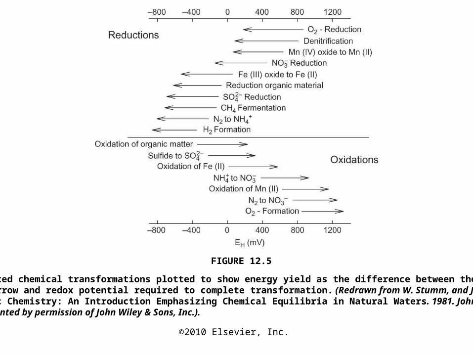
FIGURE 12.5

Microbe-mediated chemical transformations plotted to show energy yield as the difference between the tail and the head of the arrow and redox potential required to complete transformation. (Redrawn from W. Stumm, and J. J. Morgan, Aquatic Chemistry: An Introduction Emphasizing Chemical Equilibria in Natural Waters. 1981. John Wiley & Sons, Inc. Reprinted by permission of John Wiley & Sons, Inc.).

©2010 Elsevier, Inc.

FIGURE 12.6

Temporal patterns of temperature, O2, redox, and total iron in Esthwaite Water (an English lake) over a year. This type of figure is common for representing time series in lakes. The contours represent the boundaries of the values, with depth on the y axis and time on the x axis. (Redrawn from Mortimer, 1941).

©2010 Elsevier, Inc.

FIGURE 12.7

Saturation concentrations of dissolved O2 as a function of temperature and altitude. The equation that describes the curve is: ln (O2) 5 2.692 2 1.27 3 1024 (alt) 2 6.15 3 10210 (alt)2 2 0.0286 (temp) 1 2.72 3 1024 (temp)2 2 2.09 3 1026 (temp)3, where O2 5 mg L21, alt is altitude in meters, and temp is temperature in °C. (equations modified from Eaton et al., 1995).

©2010 Elsevier, Inc.

FIGURE 12.8

Diagram of a representative relationship between net photosynthetic rate and irradiance (A) and comparison of

high-light- and low-light-adapted species (B). The low-light species has a steeper α, lower compensation point and Pmax, and greater photoinhibition. Irradiance is in photosynthetically available radiation, and photosynthetic rate is in arbitrary units. A single species can acclimate to light in a similar fashion.

©2010 Elsevier, Inc.

FIGURE 12.9

Relationship between photosynthetic rate and temperature based on 94 measurements of stream epilithon production in 14 studies. (Reproduced with permission from DeNicola, 1996).

©2010 Elsevier, Inc.

FIGURE 12.10

Relationship between water velocity and photosynthetic rate of the benthic cyanobacterium Nostoc. (From Dodds, 1989, with permission of the Journal of Phycology).

©2010 Elsevier, Inc.

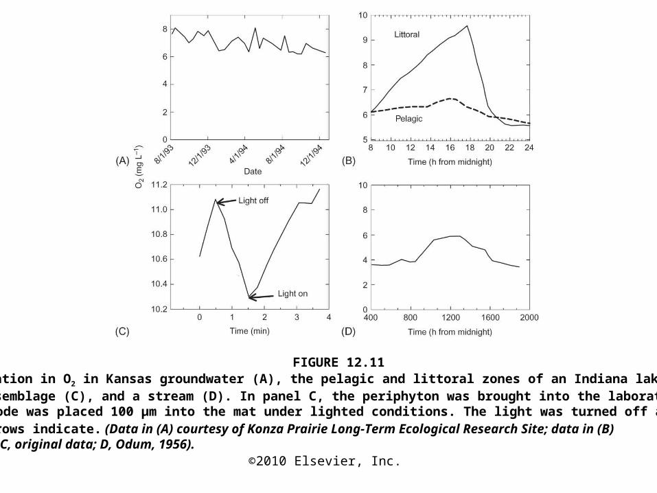
FIGURE 12.11Temporal variation in O2 in Kansas groundwater (A), the pelagic and littoral zones of an Indiana lake (B), a periphyton assemblage (C), and a stream (D). In panel C, the periphyton was brought into the laboratory, and an O2 microelectrode was placed 100 μm into the mat under lighted conditions. The light was turned off and back on where the arrows indicate. (Data in (A) courtesy of Konza Prairie Long-Term Ecological Research Site; data in (B) from Scott, 1923; C, original data; D, Odum, 1956).

©2010 Elsevier, Inc.

FIGURE 12.12

Robert Wetzel.

©2010 Elsevier, Inc.

FIGURE 12.13

O2 profiles from the stratified Triangle Lake, Oregon, on October 1, 1983, mid-morning (A) and from the South Saskatchewan River in an active algal mat, midday on June 9, 1993 (B). Note the lack of O2 in the hypolimnion and the possible deep photosynthetic activity (at 10–14 m) that causes a slight increase in O2 in panel A and the supersaturating O2 concentration at the sediment surface in panel B. (Data for panel A courtesy of R. W. Castenholz; data for B from Bott et al., 1997).

©2010 Elsevier, Inc.

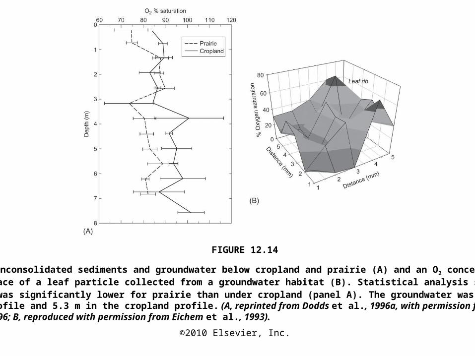
FIGURE 12.14

O2 profiles in unconsolidated sediments and groundwater below cropland and prairie (A) and an O2 concentration map at the surface of a leaf particle collected from a groundwater habitat (B). Statistical analysis showed that the O 2

concentration was significantly lower for prairie than under cropland (panel A). The groundwater was at 4.2 m in the prairie profile and 5.3 m in the cropland profile. (A, reprinted from Dodds et al., 1996a, with permission from Elsevier Science, 1996; B, reproduced with permission from Eichem et al., 1993).