The Value and Applicability of Bargaining in an

Intergenerational Setting

Gregory Howard*

Doctoral student

Department of Agricultural, Environmental, and Development Economics

Ohio State University

103 Agricultural Administration Building

2120 Fyffe Road

Columbus, OH 43210

Howard.761@buckeyemail.osu.edu

Selected Paper prepared for presentation at the Agricultural & Applied Economics

Association’s 2011 AAEA & NAREA Joint Annual Meeting, Pittsburgh, Pennsylvania, July

24-26, 2011

Copyright 2011 by Gregory Howard. All rights reserved. Readers may make verbatim copies of

this document for non-commercial purposes by any means, provided that this copyright notice

appears on all such copies.

* I thank my advisors, Tim Haab and Brian Roe, for helpful guidance and suggestions. I also thank Ben Anderson,

Carolina Castilla, Afif Naeem, and Carlianne Patrick for helpful comments, as well as seminar participants at Ohio

State University and the 2011 Midwest Economic Association Annual Conference. Financial support from the

Environmental Policy Initiative is gratefully acknowledged.

Abstract

This paper considers the effectiveness of a variation of Coasian bargaining as a policy

instrument for internalizing one or multiple intergenerational externalities. The variation

involves appointing a contemporary party to represent the interests of the affected parties who

are currently unable to represent themselves, either because they are too young or have not yet

been born. Potential criticisms of such a policy are considered and addressed, and precedents to

such a policy are put forth.

To test the value of such a policy, a two-period model in which two externalities exist in

the production/consumption decisions and with representative agents is used to compare the

welfare effects of four scenarios: 1) The agent in each period chooses allocations to maximize

utility in that period, 2) a benevolent social planner chooses allocations in both periods to

maximize a social welfare function, 3) the government assigns and enforces property rights and

acts as an intermediary in negotiations to determine allocations in each period, and 4) agents

choose allocations to maximize period-specific utility subject to a tax-and-subsidy regime

imposed by the government. The four scenarios are solved and comparative statics are analyzed

analytically where possible and through simulations when the model become analytically

intractable. The model is tested for robustness through sensitivity analysis of the model

parameters, adjusting the functional form of the social welfare function, and extending the model

to three periods.

I find that, contrary to general consensus in the literature, Coasian bargaining can be

adapted in such a way as to make it applicable in an intergenerational framework. In addition, I

find that the welfare outcomes of the Coasian bargaining scenario are marginally lower but

comparable to that of the tax-and-subsidy regime, and that both policy instrument scenarios have

similar comparative statics and sensitivity analyses. The main disparity between the two policy

regimes pertains to how increasing the effectiveness of research and development (R&D)

changes the optimal level of R&D. The tax-and-subsidy scenario finds that there is a positive

relationship between this parameter and the equilibrium level of R&D, while the bargaining

scenario yields a negative relationship.

1

Section 1: Introduction

When dealing with externalities that exist between two or more contemporary agents, the

environmental economic literature has recognized many different methods of internalizing the

external cost in order to achieve efficient outcomes (For a comparison of these different policies

under uncertainty, see Weitzman (1974)). These methods range from regulating prices through

taxes and subsidies (Pigou 1952, Cornes and Sandler 1985, Wittman 1985), to regulating

quantities through quotas and cap and trade, to more “decentralized” methods like Coasian

bargaining (Coase 1960). However, when attempting to resolve issues such as global warming,

the use of nuclear power, and biodiversity loss, the relevant externalities are not limited to the

current population, but instead extend to agents in future generations.

Coasian bargaining is generally considered an infeasible policy option when dealing with

intergenerational externalities as it relies on negotiations between parties separated by decades

(or even centuries). Padilla (2002) said, in reference to market solutions to intergenerational

externalities, “In particular, the ‘Coasian’ analysis is out of place: there is no possible agreement

between the parts because future generations are not present nor represented either.” (p. 72). This

is a legitimate objection, and it focuses on the decentralized nature of Coasian bargaining. We

face a permanent and inflexible constraint in which we are unable to move freely through time as

we do space. This constraint seems to irrevocably damn decentralized bargaining, as well as any

other potential decentralized policies, when the problem is intergenerational in nature. However,

decentralization is only half of the Coasian bargaining story. The feasibility of a decentralized

bargaining policy is dependent on not just the possibility of decentralization (meaning the

“policy” is implemented by the effected parties and not the government), but also on the ability

of these parties to bargain. This bargaining aspect is the baby that is thrown out with the

2

decentralization bath water. Because decentralization and bargaining are tied so closely in the

minds of economists, the profession often fails to consider the possibility of having one without

the other.

One might be incredulous toward any bargaining scheme in which the two affected

parties have no chance to negotiate. The future cannot sit opposite the present at any negotiating

table. However, should it be possible for a contemporary party to represent the interests of the

future, bargaining could once again be viable. If this party was the government, we would not be

engaging in Coasian bargaining per se, but instead in centralized bargaining. Having today’s

government represent a faceless future that does not yet exist is enough to raise further

objections (for example, how can today’s government presume to know the preferences of future

peoples?), but it would be erroneous to assume that centralized bargaining is unique among

policy instruments in such weaknesses. For example, when calibrating an optimal tax aimed at

internalizing an intergenerational externality, the government must be aware of the preferences

and endowments of people who have yet to be born. If they do not know these preferences and

endowment, or if their estimates are wildly inaccurate, the chosen tax rate is likely to be far from

optimal. Thus, for any policy, bargaining or otherwise, the government must have a good

estimate of future preferences to have any chance of implementing effective policy. It is

reasonable to be skeptical about our estimates of future preferences, but such skepticism is

equally damning to policies across the board.

In addition to possessing accurate estimates of future preferences and endowments, the

government (or any party representing the future) must also be committed to representing the

best interests of the future. This assumption is likewise fair game for skepticism and credulity. It

seems unlikely that politicians will forgo the interests of their constituents in order to negotiate

3

forcefully and effectively for parties who have no say in their reelection. This is the “missing

voter” problem addressed by Doeleman and Sandler (1998). If this is true, centralized bargaining

will not be effective. However, assuming that the government doesn’t actually care about the

future causes ALL policies aimed at internalizing intergenerational externalities to be ineffective,

not just centralized bargaining. If politicians care only about the interests of their constituents,

not only would bargaining policies fail, but any regulation of quantity or price will fail in similar

fashion. What hope is there for effective Cap and Trade legislation or carbon taxes that

accurately reflect the social cost of carbon when the government is unconcerned about the

interests of future generations, who are the beneficiaries of such action1? There is none.

It is also reasonable to suggest that transaction or information costs can be prohibitive

when it comes to bargaining outcomes. In the case of many heterogeneous parties negotiating on

either or both sides, it is likely that the costs of negotiating are high. Similarly, the existence of

private information can lead to parties “holding out” in negotiations and failing to achieve

efficient outcomes (Farrell 1987). Clearly, the existence of these real world frictions relegates

any bargaining policy to the world of second best outcomes. However, the same is undoubtedly

true for price and quantity regulations, as the cost of acquiring information on preferences, as

well as the cost of monitoring and enforcement, is certainly nonzero and in many cases

substantial. The question, then, is not whether bargaining policies are in all cases efficient or

superior to price and quantity alternatives, but rather whether bargaining policies are comparable

to these alternatives given the right circumstances.

1One could argue that governments could appear to care about future generation, without actually doing so, by

levying a tax to correct a contemporaneous externality if said tax has the unintended consequence of being beneficial

to future generations. If, however, a tax was purely detrimental to the present and beneficial to the future, this caveat

would not hold. In addition, even if the externality affects both contemporary and future parties, a tax that takes into

account only the interests of contemporary parties will not be an optimal tax.

4

The concept of assigning property rights to future generations in order to protect their

interests is not new. Pasqual and Souto (2003) argue that the assignment of resource rights can

help alleviate externalities between generations. They also consider various property rights

assignments and their respective implications for sustainability. The work of this paper deviates

from these previous efforts in several ways. First, this paper does not consider sustainability,

though the extension of the model presented herein to infinite periods would produce interesting

implications for sustainability. Second, Pasqual and Souto consider the property rights

assignment of a single resource that generates intergenerational externalities, while this paper

presents a model in which multiple externalities exist from multiple sources, each of which can

have rights assigned to it. Third, while previous work allows for the assignment and enforcement

of property or resource rights to the future, they do not consider the prospect of bargaining

between the present and the contemporary party representing the interests of the future.

Padilla (2002) advocates the assignment of property rights to future generations in the

interest of sustainability, arguing that failing to do so implicitly assigns property rights to the

present and is still “value laden.” (p. 75). Padilla eschews bargaining solutions as well as

“Pigouvian” solutions on the grounds that the market valuations assigned to the future are

unreliable and somewhat arbitrary. In addition, he acknowledges the “compensation rule,” in

which the present generation’s use of resources in a manner that violates the rights of future

generations should bear with it compulsory compensation from present to future (how to

determine appropriate compensation in the face of unreliable and arbitrary information is left

unclear). This is similar to Bromley’s (1989) liability rule. Padilla also advocates the

development of institutions “acting as representatives, defenders, and tutors,” of future

generations’ rights (2002, p. 80).

5

While there is no clear precedent in favor of representing the interests of future

generations as a matter of policy, it is standard practice to appoint parties to represent the

interests of children in both custody (Parley 1993) and neglect/abuse proceedings (Elrod 1995-

1996). In this context, the policy tool suggested in this paper is akin to appointing a class-action

guardian for future generations. In addition, it is common practice among many Native American

tribes, both historically and today, to consider the impact of any decision on the next seven

generations of the tribe (Trosper 1995). While such a system is not identical to the one proposed

in this paper, as it involves no bargaining, it is similar in its intention of internalizing

externalities affecting unborn generations.

The purpose of this paper is to demonstrate the usefulness of Coasian bargaining in the

case of multiple intergenerational externalities. For the remainder of this paper, the term Coasian

bargaining refers to bargaining in which a contemporary agency represents the interests of the

future. This agency could be the government, in which case Coasian Bargaining is a misnomer.

However, this agency can also be decentralized. For instance, in an attempt to protect

biodiversity, organizations like the Sierra Club or the WWF could potentially represent the

interests of the future in negotiations. The model that follows considers an economy with

multiple externalities. This is done for two reasons. First, this is more realistic. Whether we like

it or not, externalities abound, especially when taking an intergenerational outlook. Just as GHG

emissions, biodiversity loss, and deforestation generate negative externalities, R&D research,

carbon sequestration, and investing in education generate positive externalities. In addition,

multiple externalities are examined because in a model with a single externality, the method of

payment in bargaining situations is purely monetary. For all intents and purposes (especially if

we are considering centralized bargaining), this is not much different from a tax. A model with

6

multiple externalities, on the other hand, provides additional methods of compensation between

the parties.

I develop a two period model (period 1 being the present and period 2 being the future) in

which the choices of the present generate two externalities, one positive and one negative, for the

future. I then solve the model under four different scenarios: 1) The representative agent in each

period chooses allocations to optimize his own utility, 2) a benevolent social planner chooses

allocations to maximize a social welfare function, 3) a Coasian bargaining scenario in which the

present and future negotiate, through a government intermediary, to determine allocations, and 4)

a tax-and-subsidy regime in which the government taxes the source of the negative externality

and subsidizes the source of the positive externality. I compare the equilibria and comparative

statics of these four scenarios, analytically where possible and using simulations when the

problem becomes analytically intractable.

One obvious conclusion from this paper is that the planner’s optimization produces

significantly greater social welfare than does the individual period optimizations. In general, the

Coasian bargaining solution does not achieve the first-best outcome, but is still significantly

superior to the individual optimization scenario. I also find that the tax-and-subsidy regime is

likewise superior to the individual optimization and marginally outperforms the Coasian

bargaining regime, but not to the extent that it is justifiable to dismiss the Coasian bargaining

regime out of hand when considering policy instruments.

The rest of the paper proceeds as follows. Section 2 presents the elements of the model.

Section 3 solves the model in the case of individual periods optimizing separately and compares

this equilibrium with equilibrium allocations derived from a social planner’s problem. Section 4

7

solves the model using the Coasian bargaining framework of assigning property rights and

entering into negotiations to decide the final allocations in the economy. Section 5 introduces

and solves for a tax-and-subsidy regime. Section 6 presents a numerical analysis with which to

compare the four scenarios. This section also provides sensitivity analyses for the parameters of

the model, adjusts the functional form of the social welfare function, and extends the model to

three periods in order to test for model robustness. Section 7 concludes and suggests possible

extensions.

Section 2: Model

The model consists of a closed economy where agents produce a composite consumption

good over two periods, t = 1, 2. Each period has one representative agent who exists for that

period only. While each period has its own representative agent, all agents across periods are

identical in their preferences, production function, and total labor endowment L. For simplicity I

assume agents do not value leisure. They allocate their labor between resource extraction, Lr, and

final good production, Lf. Resource extraction is a linear function of labor and follows:

rt = r(Lrt) = Lrt, (1)

Where rt is the resources extracted for use in period t, so one unit of labor extracts one unit of

resource. The resource stock available in the following period is defined as Rt+1 = Rt – rt. The use

of resources in the production process generates pollution, which has a deleterious effect on

welfare in future periods. The use of the resource in final good production generates pollution at

a constant one-to-one rate, while pollution already in existence dissipates, giving rise to the

pollution growth function

8

Pt+1 = δPt + rt, (2)

where Pt is pollution in period t and 0 ≤ δ ≤ 1. This may seem like a strong assumption, but it is

based on a reasonable argument. Clearly an agent will not commit labor to extract resources and

then not use the resources in production, so resources extracted will always equal resources used

in production. Assuming the resource is homogeneous, the first unit used should not produce

more pollution than the nth

unit. The one assumption that is unrealistic is the assumption that the

marginal productivity of labor in resource extraction is constant. This assumption was made for

simplicity and could be relaxed in future manifestations of this model. Production in each period

is Cobb-Douglass and exhibits constant returns to scale. Production takes the form

Yt = F(Lft , rt) = TtLftαrt

1 – α = TtLft

αLrt

(1 – α). (3)

In this formulation 0 < α < 1 and Tt represents total factor productivity in period t. Output can be

used as either current consumption or invested in research and development (R&D), Yt = Ct + At,

where Ct is consumption and At is R&D spending in time period t. Consumption represents the

benefit of production for the current population, while R&D reflects production that improves

total factor productivity for future periods. In this way, TFP evolves according to the rule

Tt+1 = γTt + ρAt, (4)

Where γ > 1 reflects advances in TFP that occur even in the absence of R&D and ρ reflects the

marginal contribution of research and development to TFP. While I acknowledge that assuming

R&D spending benefits only the future is at best tenuous and more likely highly inaccurate, such

an assumption is made for the sake of model simplicity and exists without loss of generality. The

important (and certainly not groundbreaking) finding regarding R&D spending is that the social

planner will choose a level of R&D spending higher than the level chosen by an individual

9

optimizer. If the social planner allocates X units to R&D, it makes no real difference whether the

private optimizer allocates zero or X/2, the basic qualitative finding is the same.

Utility in each period is given by the utility function

Ut(Ct, Pt) = log(Ct) – D(Pt) = log(Yt – At) – φPt1+θ

, (5)

Where D(.) is the pollution damage function and U(.) is monotonically increasing and concave

in its first argument. θ > 0, which implies that damages are convex in Pt. Convexity of the

environmental damage function is a common assumption of the literature (see, for example,

Babu, Kavi Kumar, and Murthy 1997). Often environmental quality enters positively and

concavely into the utility function. This is equivalent to a convex environmental quality damage

function. I also considered the model assuming values of θ between -1 and 0, reflecting strict

concavity of the environmental damage function, and the results were not significantly different.

Additionally and without loss of generality, we assume that P1 = 0. We also assume that R1 is

sufficiently large so that resource constraints will not bind in either period.

Section 3: Individual and Planner Optimizations

In this section, I examine two possible outcomes: that of the agent in each period

optimizing their individual utility function and that of a social planner optimizing an additive

combination of welfare for both periods. In the individual optimization scenario, the first period

faces the following problem:

���Lf1, Lr1, A1

{log(T1Lf1αLr1

(1 – α) – A1)}, (6)

10

subject to Lf1 + Lr1 ≤ L,

0 ≤ A1, Lf1, Lr1.

In this scenario, the constraint on A1 is binding, so no R&D spending occurs in equilibrium. The

first order conditions for Lf1 and Lr1 are as follows:

Lf1: αT1Lf1

α – 1Lr1(1 – α)

T1Lf1αLr1

(1 – α) – A1

= µ, (7)

Lr1: (1-α)T1Lf1

αLr1 – α

T1Lf1αLr1

(1 – α) – A1

= µ, (8)

where µ is the Lagrange multiplier for the labor constraint. Combining equations (7) and (8), we

derive the following equality:

(1-α)T1Lf1αLr1

–α = αT1Lf1

α – 1Lr1

(1 – α). (9)

Explicit values for Lf1 and Lr1 are easily found and shown in the appendix, but the important

result is that period 1 allocates labor so as to equate the marginal products of the two labor

choices, MPLf1 = MPLr1. Period 2 is faced with a similar, but not identical, optimization

problem:

���Lf2, Lr2, A2

{ log(γT1Lf2αLr2

(1 – α) – A2) – φLr1

(1+θ)}, (10)

subject to Lf2 + Lr2 ≤ L,

0 ≤ A2, Lf1, Lr1.

11

Once again, I find that the R&D constraint binds, leaving A2 equal to zero. In addition, period 2

will also allocate labor in a manner that equates the marginal product of Lf2 with the marginal

product of Lr2.

I turn next to the central planner’s problem. The goal of the central planner is defined

here as maximizing the weighted sum of period-specific utilities. This can be formally written as

���� �,���,��,Lf2, Lr2, A2

{ log(T1Lf1αLr1

(1 – α) – A1) +

β[log((γT1 + ρA1)Lf2αLr2

(1 – α) – A2) – φLr1

(1+θ)]} (11)

Subject to Lf1 + Lr1 ≤ L,

Lf2 + Lr2 ≤ L,

0 ≤ A1, A2, Lf1, Lr1, Lf2, Lr2.

In this formulation, β is the weight assigned to period 2 and the weight assigned to period 1 is

normalized to 1. I use the term “weighted sum,” as opposed to “discounted sum” because I put

no restrictions on the value of β. The typical restriction in the literature is β < 1. This is

sometimes due to mathematical necessity and sometimes stems from the observation that

individuals tend to discount future consumption. In either case, I find it an unnecessary

assumption for the purposes of this model.

As is demonstrated in the appendix, the planner’s allocation of labor and R&D in period

2 is identical to the allocations achieved using the individual optimization method. There is,

however, an important difference in period 1 allocations between the two solution methods,

assuming β ≠ 0 (If β = 0, the planner’s problem becomes equivalent to the problem faced by

12

period 1 in the individual optimization problem). This divergence can be seen by considering the

first order condition with respect to Lr1,

(1-α)T1Lf1

αLr1 –α

T1Lf1αLr1

(1 – α) – A1

= µ1 + β φ(1 + θ)Lr1θ. (12)

In this formulation, µ1 is the Lagrange multiplier associated with the period 1 labor constraint.

Combining equation (12) with the first order condition with respect to Lf1 (which is identical to

the result in the individual optimization example, equation (7)) yields a new maximization

condition:

(1-α)T1Lf1

αLr1–α

T1Lf1αLr1

(1 – α) – A1

= αT1Lf1

α – 1Lr1(1 – α)

T1Lf1αLr1

(1 – α) – A1

+ β φ(1 + θ)Lr1θ. (13)

A rather intuitive and well documented result can be seen from this equation. Individual welfare

maximization yields different allocations for labor than does the social planner maximization, so

long as the social planner uses a nonzero weight β. In this way, intergenerational externalities are

no different than externalities imposed upon contemporary agents. In addition to this finding, we

can derive an optimal level of A1 from the first order condition as shown below:

A1 = ρβTLf1

αLr1(1 – α) – γT

�(�� �) . (14)

Analysis of this finding enables us to state the following proposition:

Proposition 1: The equilibrium value of A1 in the social planner’s problem will be strictly

positive (and therefore different from the individual optimization scenario) provided γ <

ρβ Lf1αLr1(1 – α). In addition, the equilibrium value of A1 is negatively correlated with the

parameter γ and positively correlated with β and ρ.

13

The derivations of the comparative statics that support Proposition 1 are in the appendix.

These findings are supported by economic intuition, as one would expect that increasing the

relative weight assigned to period 2, β, places more emphasis on future welfare and results in a

higher equilibrium A1. Similarly, increasing ρ (the marginal increase in TFP from R&D

spending) increases the marginal future gains from research and development, and as such

increases in ρ result in greater equilibrium A1. Lastly, increasing γ (the multiplicative increase in

TFP in the absence of R&D) while keeping ρ constant decreases the productivity gains from

R&D relative to the baseline productivity gains achieved without R&D spending. In other words,

increasing γ makes the future better off, and as such the need for R&D spending is lessened and

equilibrium A1 falls. In addition to the externality produced by the resource, the planner’s

scenario corrects the externality related to research and development. When optimizing

individually, the first period underinvests in R&D, just as they overexploit the resource.

As mentioned earlier, setting β = 0 collapses the planner’s problem into the period 1

individual optimization problem. Setting β = 0 in equation (14) returns a negative number.

Combining this finding with the nonnegativity constraint presented in equation (11) yields an

equilibrium level of R&D spending of zero, the same result found in the individual optimization

problem.

Equations (13), (14), and the labor constraint give us three equations which we can use to

find equilibrium solutions for the three variables in question: A1, Lf1, and Lr1. The equilibrium

values cannot be obtained analytically, but instead must be derived using numerical methods.

This will be done for a variety of parameter values in Section 6.

14

Section 4: Coasian Bargaining

I now assume the existence of a societal agency that can assign and enforce property

rights between different generations. Such an agency is not far-fetched, as governments routinely

protect natural resources, such as forestry and wildlife, in order to ensure their existence for

future generations. This, in essence, this is equivalent to the assignment of property rights to

agents in the future. We will also assume that this agency performs its duties at no cost.

This agency could assign the resource rights to either period 1 or period 2. The pattern of

property rights assignment has important welfare and equity implications for the model (for a

more detailed elaboration, see Howarth and Norgaard 1990). In the context of our current model,

it makes more sense to assign the resource rights to period 2 for several reasons. First, the model

is composed in such a manner as to leave period 2 no means to pay period 1 in exchange for the

right to use resources (There are, of course, viable methods of compensation from the future to

the present, foremost among them being the ability of the present to acquire deficits that must be

paid off by the future). In addition, there is reason to believe that compensation should be paid

by the party that is imposing the externality, in this case period 1, rather than by the “victim.”

This is known as the polluter pays principle (Conversely, it may also be argued that productivity

gains will make the future more affluent than their present counterparts, and as such the future is

in a better position to bear the weight of compensation). Lastly, a positive externality exists in

the model in the extent to which period 1 engages in R&D. By assuming that period 1 is under

no obligation to generate research and development, I implicitly assign property rights to period

1 (i.e. the right to not engage in R&D). By assigning the resource rights to the future, I am

assigning one set of rights to each period.

15

Once property rights have been accordingly assigned, I model negotiations between

periods in the form of an ultimatum game similar to Schweizer (1988) in which the period 1

agent makes an offer (A1, r1) and the agency, representing the interests of the period 2 agent, can

either accept or reject. In the offer, compensation will be paid to period 2 in the form of

increased levels of period 1 R&D. This will be accompanied by period 2 granting the right of

period 1 to extract and use a specified amount of the resource, r1. Because period 2 controls the

resource property rights and the resource stock is sufficiently large, the optimal allocation for

period 2 will be identical to the allocations found in the previous section of the paper. Period 2

will accept any offer so long as the resultant utility from accepting the offer is greater than or

equal to the utility achieved without the offer. Formally, the offer must satisfy the following

condition:

log((γT1 + ρA1)Lf2αLr2

(1 – α)) – φr1

(1 + θ) ≥ log(γT1Lf2

αLr2

(1 – α)). (15)

Rearranging this condition, period 2 will accept any offer (r1, A1) that satisfies

r1 ≤ φ-1

(log[ (γT1 + ρA1)

γT1])

1/(1 + θ). (16)

This equation can be rewritten to solve for A1 and combined with equation (1) to yield

A1 ≥ [γT1exp(φLr1(1 + θ)

) – γT1]/ρ. (17)

Because period 1 gets no direct benefit from A1, this will hold with equality.

The comparative statics (see appendix for derivations) for equation (17) allow me to

make the following proposition:

16

Proposition 2: The equilibrium value A1 in the Coasian bargaining scenario is increasing in Lr1

and γ (the multiplicative increase in TFP in the absence of R&D) and is decreasing in ρ

(the marginal increase in TFP from R&D spending).

This is an interesting finding, as the comparative statics for γ and ρ in the social planner’s

problem were decreasing and increasing, respectively. This difference can be explained by

considering the different goals of the decision makers in each problem. In the planner’s problem,

the planner chooses a level of R&D in which the marginal benefits of research and development

equal the marginal costs. Increasing ρ in this case increases the marginal benefits without

affecting the marginal costs to the present, and as such A1 increases with ρ. Conversely,

increasing γ decreases the marginal effectiveness of R&D spending due to the concavity of the

utility function, and as such A1 decreases with increases in γ. In the Coasian bargaining solution

the equilibrium equation is set by the agent in period 1. Her goal is to equalize the total benefits

of R&D with the total damages incurred in period 2 from resource use in period 1.2 In this case,

increasing ρ increases the total benefits of A1, so for a given level Lr1 the amount of R&D

spending needed to equalize total benefits and damages is lower. Increasing γ, on the other hand,

effectively decreases the utility gained from a given level of R&D spending. As a result, period 1

must offer a greater level of A1 to equalize utility gains with utility losses for period 2. Ergo,

increasing γ increases equilibrium A1.

Using equation (17), which I will call the acceptance constraint, I can now articulate the

maximization problem faced by period 1:

2 In a world where the resource constraint is binding, Period 1 must set the total benefits of R&D equal to the total

damages in period 2 resulting from period 1 using the resource plus the disutility from lost production in period 2

due to the transfer of resources to period 1.

17

���� �,���

{ log[T1Lf1αLr1

(1 – α) – (γT1exp(φLr1

(1 + θ)) – γT1)/ρ]} (18)

Subject to Lf1 + Lr1 ≤ L,

0 ≤ Lf1, Lr1.

The first order conditions are as follows:

Lf1: ραT1Lf1

α – 1Lr1(1 – α)

ρT1Lf1αLr1

(1 – α) – (γT1exp(φLr1(1 + θ)) – γT1)

= µ, (19)

Lr1: ρ(1-α)T1Lf1

αLr1–α – γTφ(1 + θ)Lr1

θexp(φLr1(1 + θ))

ρT1Lf1αLr1

(1 – α) – (γT1exp(φLr1(1 + θ)) – γT1)

= µ. (20)

Solving for µ leaves two variables (Lr1 and Lf1) and two equations (a combination of equations

(19) and (20) as well as the labor constraint). The equilibrium solutions for these variables

cannot be solved analytically, but they are obtained through numerical methods in Section 6.

Section 5: Tax and Subsidy Regime

I will now consider the equilibrium allocation of labor and R&D when a different policy

instrument is being used, specifically a tax and subsidy regime. In this policy, the government

will levy a per-unit tax τ on resource use in the present. The revenue from this tax will then be

invested in research and development. The agent in each time period optimizes individually, but

takes the government’s tax/subsidy as given. We assume that the government can see the optimal

response to the tax from both periods and can use this knowledge to choose a tax level that

maximizes the government’s social welfare function (SWF), which we take to be equivalent to

18

the social planner’s SWF outlined in Section 3. In this case, period 1 faces the following

optimization problem:

maxLf1, Lr1, A1Log(TLf1

αLr1

1 – α – τLr1 − A1), (21)

Subject to Lf1 + Lr1 ≤ L,

0 ≤ A1, Lf1, Lr1 .

As in the individual optimization scenario, the chosen level of A1 will be zero. The other two

first order conditions can be combined to yield the following equality:

αTLf1α – 1

Lr11 – α

= (1 – α)TLf1αLr1

-α – τ. (22)

This equation shows that the optimal distribution of labor in period 1 depends on the tax rate τ.

The allocations of Lf2, Lr2, and A2 are not influenced by τ. A demonstration of this is included in

the appendix.

The government is then faced with the following optimization problem:

max {Log[TLf1(τ)αLr1(τ)

1 – α – τLr1(τ)] +

β(Log[(γT + ρτLr1(τ))Lf2(τ)αLr2(τ)

1 – α] – φLr1(τ)

1 + θ), (23)

Subject to 0 ≤ τ.

This problem can equivalently be written:

max� �,���,τ Log[TLf1αLr1

1 – α – τLr1] +

β(Log[(γT + ρτLr1)Lf2αLr2

1 – α] – φLr1

1 + θ), (24)

19

Subject to Lf1 + Lr1 ≤ L,

αTLf1α – 1

Lr11 – α

= (1 – α)TLf1αLr1

-α – τ.

This optimization problem cannot be solved analytically. However, using the second constraint

in equation (24) I can eliminate τ in the maximization problem. After doing so, the first order

conditions are as follows:

Lf1: αTLf1

α – 1Lr11 – α – α(1 – α)TLf1

α – 1Lr11 – α + α(α – 1)TLf1

α – 2Lr12 – α

αTLf1αLr1

1 – α + αTLf1α – 1Lr1

2 – α +

β[ρ(α(1 – α)TLf1

α – 1Lr11 – α – α(α – 1)TLf1

α – 2Lr12 – α)]

γT + ρ[(1 – α)TLf1αLr1

1 – α – αTLf1α – 1Lr1

2 – α] = µ, (25)

Lr1: (1 – α)TLf1

αLr1-α – (1 – α)2TLf1

αLr1-α + α(2 – α)TLf1

α – 1Lr11 – α

αTLf1αLr1

1 – α + αTLf1α – 1Lr1

2 – α +

β[ρ[(1 – α)2TLf1

αLr1-α – α(2 – α)TLf1

α – 1Lr11 – α]

γT + ρ[(1 – α)TLf1αLr1

1 – α – αTLf1α – 1Lr1

2 – α] - φ(1 + θ)Lr1

θ] (26)

=µ,

where µ is the Lagrange multiplier for the labor constraint. Solving for µ leaves two variables

and two equations (a combination of (25) and (26) as well as the labor constraint). The

equilibrium allocations cannot be solved analytically, but may be solved using numerical

methods.

Section 6: Numerical Methods and Robustness

20

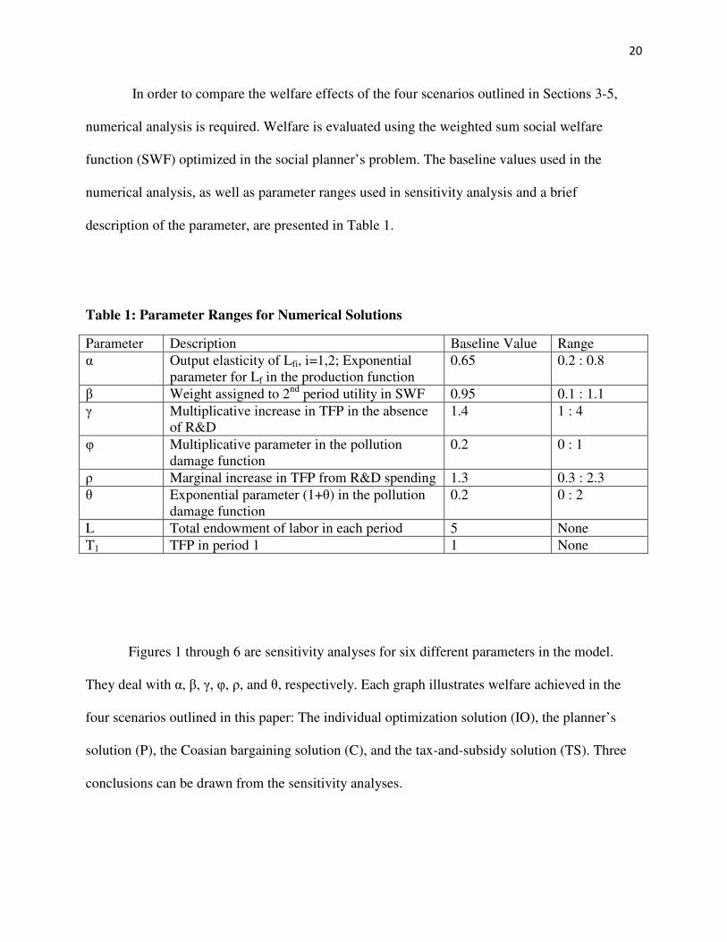
In order to compare the welfare effects of the four scenarios outlined in Sections 3-5,

numerical analysis is required. Welfare is evaluated using the weighted sum social welfare

function (SWF) optimized in the social planner’s problem. The baseline values used in the

numerical analysis, as well as parameter ranges used in sensitivity analysis and a brief

description of the parameter, are presented in Table 1.

Table 1: Parameter Ranges for Numerical Solutions

Parameter Description Baseline Value Range

α Output elasticity of Lfi, i=1,2; Exponential

parameter for Lf in the production function

0.65 0.2 : 0.8

β Weight assigned to 2nd

period utility in SWF 0.95 0.1 : 1.1

γ Multiplicative increase in TFP in the absence

of R&D

1.4 1 : 4

φ Multiplicative parameter in the pollution

damage function

0.2 0 : 1

ρ Marginal increase in TFP from R&D spending 1.3 0.3 : 2.3

θ Exponential parameter (1+θ) in the pollution

damage function

0.2 0 : 2

L Total endowment of labor in each period 5 None

T1 TFP in period 1 1 None

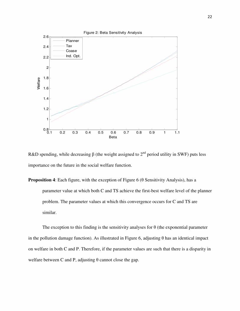
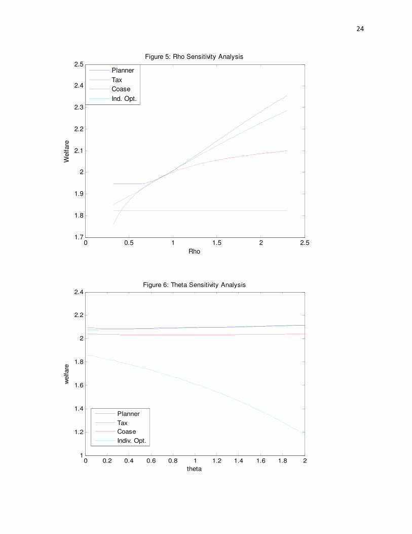
Figures 1 through 6 are sensitivity analyses for six different parameters in the model.

They deal with α, β, γ, φ, ρ, and θ, respectively. Each graph illustrates welfare achieved in the

four scenarios outlined in this paper: The individual optimization solution (IO), the planner’s

solution (P), the Coasian bargaining solution (C), and the tax-and-subsidy solution (TS). Three

conclusions can be drawn from the sensitivity analyses.

21

Proposition 3: both the TS regime and the C regime are significant improvements over the IO

solution. The welfare achieved in IO rivals that of TS and C only in two instances: very

low values of ρ and very low values of β.

This outcome makes intuitive sense. The individual optimization scenario leads to no

R&D spending and heavily favors utility in the present over utility in the future. Decreasing the

value of ρ (the marginal increase in TFP from R&D spending) decreases the marginal benefit of

0.2 0.3 0.4 0.5 0.6 0.7 0.8 0.91.4

1.6

1.8

2

2.2

2.4

2.6

2.8

Figure 1: Alpha Sensitivity Analysis

Alpha

Welfare

Planner

Tax

Coase

Ind. Opt.

22

R&D spending, while decreasing β (the weight assigned to 2nd

period utility in SWF) puts less

importance on the future in the social welfare function.

Proposition 4: Each figure, with the exception of Figure 6 (θ Sensitivity Analysis), has a

parameter value at which both C and TS achieve the first-best welfare level of the planner

problem. The parameter values at which this convergence occurs for C and TS are

similar.

The exception to this finding is the sensitivity analyses for θ (the exponential parameter

in the pollution damage function). As illustrated in Figure 6, adjusting θ has an identical impact

on welfare in both C and P. Therefore, if the parameter values are such that there is a disparity in

welfare between C and P, adjusting θ cannot close the gap.

0.1 0.2 0.3 0.4 0.5 0.6 0.7 0.8 0.9 1 1.10.8

1

1.2

1.4

1.6

1.8

2

2.2

2.4

2.6Figure 2: Beta Sensitivity Analysis

Beta

Welfare

Planner

Tax

Coase

Ind. Opt.

23

1 1.5 2 2.5 3 3.5 41.5

2

2.5

3Figure 3: Gamma Sensitivity Analysis

Gamma

Welfare

Planner

Tax

Coase

Ind. Opt.

0 0.1 0.2 0.3 0.4 0.5 0.6 0.7 0.8 0.9 10

0.5

1

1.5

2

2.5Figure 4: Phi Sensitivity Analysis

phi

welfare

Planner

Tax

Coase

Indiv. Opt.

24

0 0.5 1 1.5 2 2.51.7

1.8

1.9

2

2.1

2.2

2.3

2.4

2.5Figure 5: Rho Sensitivity Analysis

Rho

Welfare

Planner

Tax

Coase

Ind. Opt.

0 0.2 0.4 0.6 0.8 1 1.2 1.4 1.6 1.8 21

1.2

1.4

1.6

1.8

2

2.2

2.4Figure 6: Theta Sensitivity Analysis

theta

welfare

Planner

Tax

Coase

Indiv. Opt.

25

Proposition 5: As each parameter moves away from the range where both policy instruments

achieve their first-best outcomes, TS tends to outperform C. The one exception is Figure

1 (α Sensitivity Analysis).

The difference is modest for all parameters except ρ (the marginal increase in TFP from

R&D spending), where the divergence in welfare between a tax-and subsidy regime and the

Coasian bargaining regime is significant. My discussion of the comparative statics for ρ in

section 4 may explain this result, as changing ρ has different marginal effects in C than it does in

P and TS. This difference is also highlighted in Figure 7, which shows that the Coasian

bargaining solution has equilibrium R&D decreasing in ρ while the Planner and Tax-and-subsidy

solutions have equilibrium R&D increasing in ρ. In addition, Figure 1 shows that C outperforms

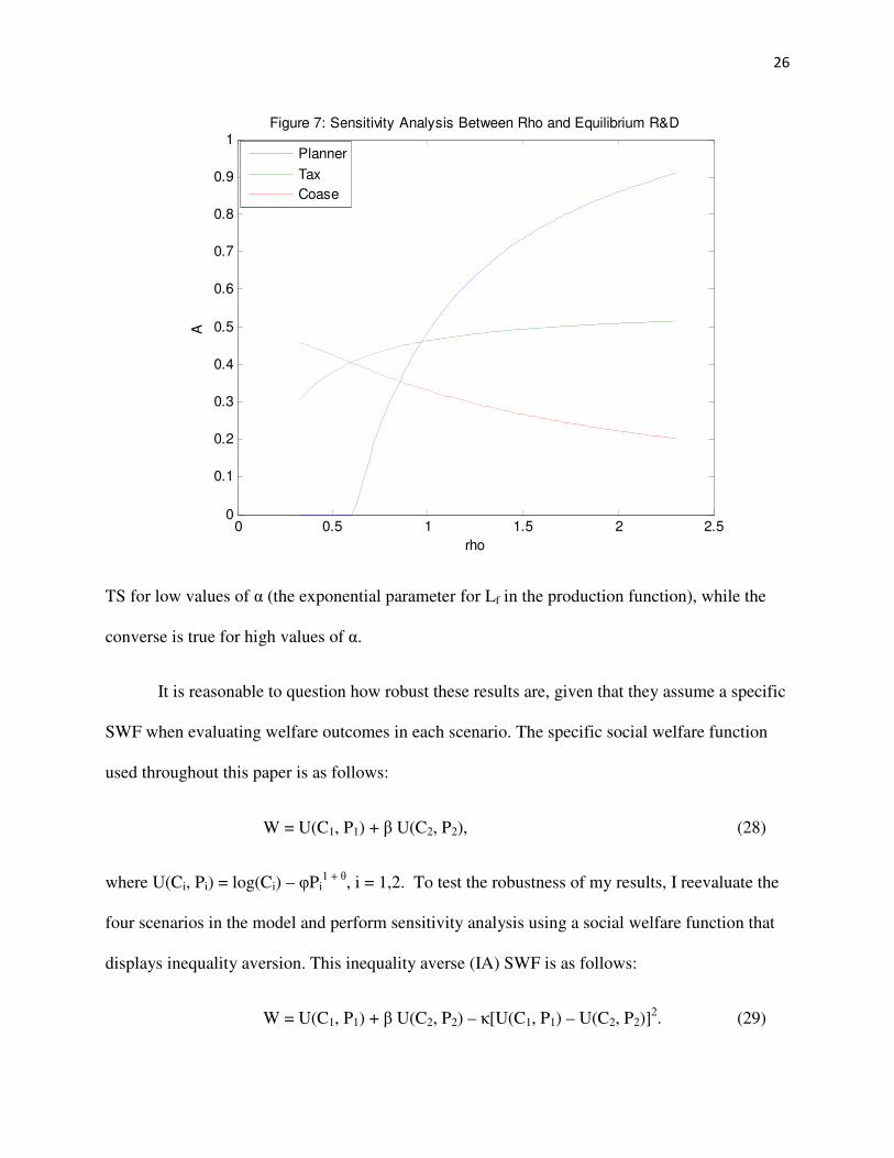
26

TS for low values of α (the exponential parameter for Lf in the production function), while the

converse is true for high values of α.

It is reasonable to question how robust these results are, given that they assume a specific

SWF when evaluating welfare outcomes in each scenario. The specific social welfare function

used throughout this paper is as follows:

W = U(C1, P1) + β U(C2, P2), (28)

where U(Ci, Pi) = log(Ci) – φPi1 + θ

, i = 1,2. To test the robustness of my results, I reevaluate the

four scenarios in the model and perform sensitivity analysis using a social welfare function that

displays inequality aversion. This inequality averse (IA) SWF is as follows:

W = U(C1, P1) + β U(C2, P2) – κ[U(C1, P1) – U(C2, P2)]2. (29)

0 0.5 1 1.5 2 2.50

0.1

0.2

0.3

0.4

0.5

0.6

0.7

0.8

0.9

1Figure 7: Sensitivity Analysis Between Rho and Equilibrium R&D

rho

A

Planner

Tax

Coase

27

Sensitivity analyses for both social welfare functions are shown side-by-side in the

appendix. The propositions put forth earlier in this section all still hold using a social welfare

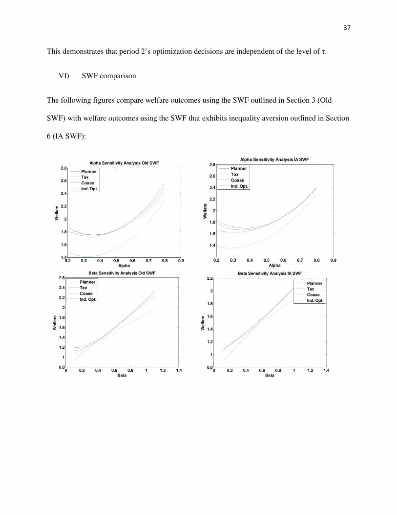
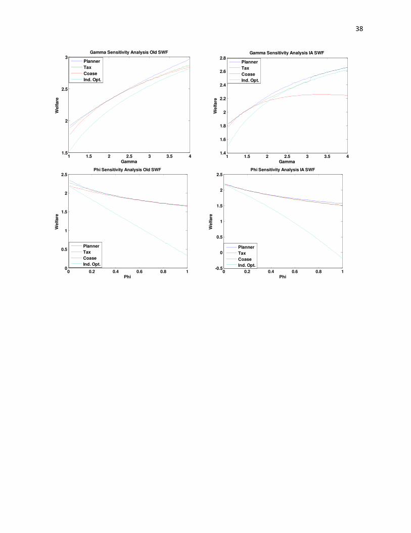
function that displays inequality aversion with a few small caveats. First, C does significantly

worse for high values of γ (the multiplicative increase in TFP in the absence of R&D) using the

IA SWF, even achieving less welfare than IO. Second, unlike with the normal SWF, C does not

outperform TS for low values of α using the IA SWF. Lastly, C does outperform TS (though not

by much) in the sensitivity analysis of θ (the exponential parameter in the pollution damage

function) using the IA SWF. With these small exceptions, the findings of this paper are borne out

even under changes in the functional form of the social welfare function, which suggests that the

results and conclusions herein are robust.

It is also reasonable to question whether the results presented above are due to the 2

period nature of the model. In order to test whether the above propositions hold when the number

of periods is increased, the model was extended by adding a third period. In doing so, relatively

few changes were necessary for the individual optimization and planner scenarios. The SWF

used in the planner and tax scenarios becomes W = U(C1) + βU(C2) + β2U(C3). For the Coasian

bargaining scenario, joint ownership of the resource in period 1 is given to the period 2 and 3

agents. This means that an offer must be made by the period 1 agent which is accepted by the

agents of both subsequent periods in order for the period 1 agent to have access to the resource.

However, this additional complication does not affect the resultant offer. This is made evident by

the following proposition:

Proposition 6: Any offer accepted by the period 2 agent will be accepted by the period 3 agent

so long as δ ≤ 1 (Proof in the appendix).

28

In period 2, ownership of the resource is given to the period 3 agent, so the period 2 and 3

agents must likewise bargain over allocation of the resource and R&D spending.

In the tax and subsidy scenario, two distinct taxes and subsidies are levied. The

government chooses the optimal tax rates, and by extension the optimal subsidies, by

maximizing the planner SWF subject to resource and feasability constraints as well as the

constraints that outline how agents in periods 1 and 2 will react to taxes. For simplicity I assume

that all of the period 1 tax is immediately spent on the period 1 subsidy. The assumption is trivial

in the present model, as period 1 R&D spending is clearly more valuable to the social

planner/government than period 2 R&D spending. This is a result of period 1 R&D being

beneficial to production on both periods 2 and 3, while period 2 R&D is beneficial to production

in period 3 alone. With the introduction of additional avenues of investment with some positive

rate of return, however, this assumption may be more restrictive. While it is clear that one unit of

A1 is preferred to one unit of A2, it is possible that (1+r) units of A2 is preferred to one unit of A1,

where r is the rate of return on the alternative investment. For the purposes of the present model,

however, this is not an issue.

As can be seen in the appendix, including a third period to the model does not

significantly impact any of the findings presented above, and in fact the sensitivity analyses

performed on the main parameters are strikingly similar between the 2- and 3-period models.

This suggests that the results are not an artifact of the small number of periods, but in fact are

robust to variations of model length.

Section 7: Conclusion

29

Intergenerational externalities add a layer of uncertainty that is generally absent in their

intragenerational counterparts. In order to properly internalize such an externality, one must

make assumptions about the endowments and preferences of a party that has not yet been born.

This is true no matter what policy instrument one uses. It has, however, been argued that Coasian

Bargaining is particularly ill-equipped to handle intergenerational externalities, as negotiations

between the present and future are seen as impossible. However, the appointment of a

contemporary party to represent the interests of the future in present-day negotiations allows

bargaining policies to circumvent such difficulties. There are additional objections that may be

raised regarding the ability and willingness of any contemporary party to know and represent the

interests of the future, but I argue that these same problems also exist for any alternate policy

option. Moreover, allowing a governing body to represent the future in property rights

negotiations is appealing in the sense that it will drastically diminish transaction costs, one of the

main inhibitors of Coasian bargaining theory. Declining negotiation costs is a common outcome

whenever a governing body is able to adequately represent the interests of a large, diverse, and

widespread group.

In this paper I consider a two period model in which two externalities exist. One

externality concerns pollution created in resource extraction and production, while the other

stems from underinvestment in research and development. I show that each time period

maximizing their personal welfare leads to allocations that are different from the first-best

allocations derived using the planner’s problem. Next, I consider a Coasian bargaining situation

in which the present has the right to invest nothing in R&D while the future controls the property

rights of the resource needed for production. I derive the condition under which the equilibrium

bargaining outcome achieves allocations equivalent to the planner’s problem, as well as how

30

deviations from this condition affect both externalities. I then compare the effectiveness of

Coasian bargaining policy to a tax-and-subsidy policy. I find that, in general, the tax-and-subsidy

policy fares slightly better than the Coasian bargaining policy, but not in such a significant way

as to warrant completely dismissing Coasian bargaining as a potential policy instrument.

While it is true that the tax-and-subsidy regime marginally outperforms the Coasian

bargaining regime in my model, I do not find this to be a discouraging result. The theme and

important finding of this paper is not that Coasian bargaining is at all times a superior policy

instrument when dealing with intergenerational externalities. Rather, this paper demonstrates that

the traditional notion of Coasian bargaining, which makes no intuitive sense in intergenerational

issues, can be adapted and adjusted into a form that is feasible and, from a welfare perspective,

competitive with other potential policies. Clearly there will be issues for which the cost of

enforcing property rights will be immense, or transaction cost will be prohibitive. For these

issues, Coasian bargaining will not be feasible. However, if issues exist for which these problems

are not as pronounced and a tax or quantity regulation has proven exceedingly difficult, either

economically or politically, Coasian bargaining may be an effective and welcome alternative.

As an example, suppose a large quantity of fossil fuel was discovered on a tract of land

owned by the government. Several companies are vying for the right to extract and sell the

resource. The government is mindful of the intergenerational externalities that exist in fossil fuel

consumption, and as such wish to increase the price in an attempt to optimize the extraction path

of the resource. One method they could use to this end is to allow companies to submit bids and

accept the bid that is deemed the best for the future, provided accepting the bid is considered to

improve future welfare over letting the resource remain in the ground. These bids could contain

multiple compensation methods, from money payments to R&D spending to emissions decreases

31

in other areas of the company, so long as these compensations have a positive impact on future

welfare. In this way, the adjusted Coasian Bargaining tool has more potential flexibility than a

tax in the right situation.

This is a simple model that can be enriched in many different ways. Possible future

extensions of the model include allowing the resource constraint to bind, increasing the number

of periods in the model to some arbitrary number N or to infinity, using more general forms or

comparing additional different forms of both the individual period utility functions and the social

welfare function, and adding altruism to the period utility function. In addition to utility

functions, several other functional forms were specified, from production and extraction

functions to environmental damage functions. The model could be extended to treat these

functional forms more generally. The model could also be changed to include some form of cash

or output transfers, with transfers from the future to the present being in the form of debt

accumulated by the present and paid by the future. The model could introduce additional

frictions in the form of transaction and property rights enforcement costs for Coasian bargaining,

as well as implementation and monitoring costs for other policy instruments. The negotiations

that take place in the model could be expanded in complexity beyond that of a very basic

ultimatum game. Lastly, the basic concept underlying this model could be applied to an

overlapping generations (OLG) model form, either over a discrete or infinite time period. Each

of these extensions would introduce an additional layer of complexity that could prove

informative, both in our theoretical understanding of intergenerational externalities and in our

comprehension of the policy options we possess when addressing these externalities.

32

References

Babu, P. Guruswamy, K.S. Kavi Kumar, and N.S. Murthy. 1997. “An Overlapping Generations

Model with Exhaustible Resources and Stock Pollution.” Ecological Economics 21: 35-

43.

Bromley, D., 1989. “Entitlements, Missing Markets, and Environmental Uncertainty.” Journal of

Environmental Economics and Management 17, 181-194.

Coase, R. 1960. “The Problem of Social Cost.” Journal of Law and Economics, 3: 1-44.

Cornes, R. and T. Sandler. 1985. “Externalities, Expectations, and Pigouvian Taxes.” Journal of

Environmenal Economics and Management 12 (1): 1-13.

Doeleman, J. and T. Sandler. 1998. “The Intergenerational Case of Missing Markets and Missing

Voters.” Land Economics, 74 (1): 1-15.

Elrod, Linda D. 1995-1996. ”An Analysis of the Proposed Standards of Practice for Lawyers

Representing Children in Abuse and Neglect Cases.” Fordham Law Review, 64: 1999-

2011.

Farrell, J. 1987. “Information and the Coase Theorem.” The Journal of Economics Perspectives

1 (2): 113-29.

Howarth, R. and R. Norgaard. 1990. “Intergenerational Resource Rights, Efficiency, and Social

Optimality.” Land Economics 66 (1): 1-11.

Key, N. and Kaplan, J. 2007. “Multiple Environmental Externalities and Manure Management

Policy.” Journal of Agricultural and Resource Economics 31 (1): 115-34.

33

Padilla, E., 2002. “Intergenerational Equity and Sustainability.” Ecological Economics 41: 69-

83.

Parley, Louis I. 1993. “Representing Children in Custody Litigation.” Journal of the American

Academy of Matrimonial Lawyers, 11: 45-64.

Pasqual, J., and Souto, G., 2003. “Sustainability in Natural Resource Management.” Ecological

Economics 46: 47-59.

Pigou, A. 1952. The Economics of Welfare. London: Macmillan.

Schweizer, U. 1988. “Externalities and the Coase Theorem: Hypothesis or Result?” Journal of

Institutional and Theoretical Economics 144: 245-66.

Trosper, Ronald L. 1995. “Traditional American Indian Economic Policy.” American Indian

Culture and Research Journal, 19: 65-95.

Weitzman, M. 1974. “Prices vs. Quantities.” The Review of Economic Studies 41 (4): 477-491.

Wittman, D. 1985. “Pigovian Taxes Which Work in the Small-Number Case.” Journal of

Environmental Economics and Management 12 (2): 44-54.

Appendix

I) Equilibrium labor allocations when each period optimizes individually

Using equation (9), we can solve for Lf1 in terms of Lr1:

34

Lf1 = α

(1- α) Lr1. (A1)

Combining this with the resource constraint yields the equilibrium allocations

Lf1 = αL, (A2)

Lr1 = (1 – α)L. (A3)

Similarly, we can solve for Lf2 in terms of Lr2:

Lf2 = α

(1- α) Lr2. (A4)

Combining this with the resource constraint yields the equilibrium allocations

Lf2 = αL, (A5)

Lr2 = (1 – α)L. (A6)

II) Equilibrium allocations under the social planner

The first order conditions, in addition to equation (12), are

Lf1: αT1Lf1

α – 1Lr1(1 – α)

T1Lf1αLr1

(1 – α) – A1

= µ1, (A7)

A1: �

T1Lf1αLr1

(1 – α) – A1

= �� Lf2

αLr2(1 – α)

(γT1 + ρA1)Lf2αLr2

(1 – α) – A2

, (A8)

Lf2: βα(γT1 + ρA1)Lf2

α – 1Lr2(1 – α)

(γT1 + A1)Lf2αLr2

(1 – α) – A2

= µ2, (A9)

35

Lr2: !"1− #$(%T1 + ρ A1)Lf2

αLr2–α

(γT1 + ρA1)Lf2αLr2

(1 – α) – A2

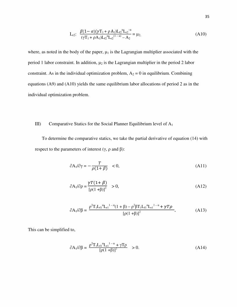
= µ2, (A10)

where, as noted in the body of the paper, µ1 is the Lagrangian multiplier associated with the

period 1 labor constraint. In addition, µ2 is the Lagrangian multiplier in the period 2 labor

constraint. As in the individual optimization problem, A2 = 0 in equilibrium. Combining

equations (A9) and (A10) yields the same equilibrium labor allocations of period 2 as in the

individual optimization problem.

III) Comparative Statics for the Social Planner Equilibrium level of A1

To determine the comparative statics, we take the partial derivative of equation (14) with

respect to the parameters of interest (γ, ρ and β):

∂A1/∂γ = − &'(1+ !) < 0, (A11)

∂A1/∂ρ = )*(�� �)

[ρ(1 +β)]2 > 0, (A12)

∂A1/∂β = ρ2T1Lf1

αLr11 – α(1 + β) – ρ2βT1Lf1

αLr11 – α � )*�

[ρ(1 +β)]2 . (A13)

This can be simplified to,

∂A1/∂β = ρ2T1Lf1

αLr11 – α + γTρ

[ρ(1 +β)]2 > 0. (A14)

36

IV) Comparative Statics for the Coasian Bargaining Equilibrium level of A1

To determine the comparative statics, we take the partial derivative of equation (17) with

respect to the parameters of interest (γ, ρ and Lr1):

∂A1/∂γ = *

� [exp(φLr1

1 + θ) – 1] ≥ 0, (A15)

∂A1/∂ρ = − %&ρ2 [exp(φLr1

1 + θ) – 1] ≤ 0, (A16)

∂A1/∂Lr1 = ρ-1γTφ(1 + θ)Lr1

θexp(φLr1

1 + θ) > 0. (A17)

In addition, equations (A15) and (A16) are strictly greater than zero if Lr1 is strictly positive.

V) Evaluating the Period 2 allocations using the tax and subsidy regime

When the government initiates a tax and subsidy regime as described in section 5, period

2 faces the following optimization problem:

maxLf2, Lr2, A2 Log[(γT + ρτLr1)Lf2

αLr2

1 – α – A2] – φLr1

1 + θ, (A18)

Subject to Lf2 + Lr2 ≤ L,

0 ≤ Lf2, Lr2, A2.

It is clear that A2 = 0. Using the first order conditions of the Lagrangian with respect to Lf2 and

Lr2 and combining them yields the equation:

Lf2 = α

(1- α) Lr2. (A19)

37

This demonstrates that period 2’s optimization decisions are independent of the level of τ.

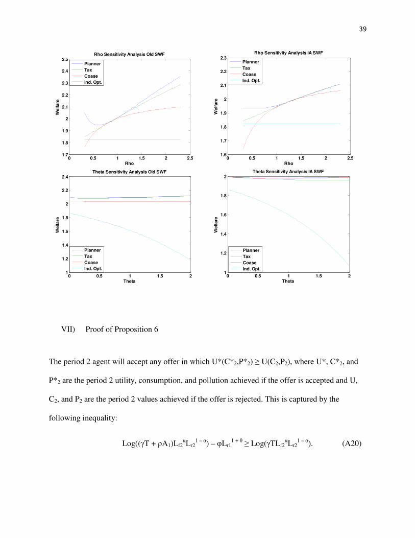
VI) SWF comparison

The following figures compare welfare outcomes using the SWF outlined in Section 3 (Old

SWF) with welfare outcomes using the SWF that exhibits inequality aversion outlined in Section

6 (IA SWF):

0.2 0.3 0.4 0.5 0.6 0.7 0.8 0.91.4

1.6

1.8

2

2.2

2.4

2.6

2.8Alpha Sensitivity Analysis Old SWF

Alpha

We

lfa

re

Planner

Tax

Coase

Ind. Opt.

0.2 0.3 0.4 0.5 0.6 0.7 0.8 0.9

1.4

1.6

1.8

2

2.2

2.4

2.6

2.8Alpha Sensitivity Analysis IA SWF

Alpha

We

lfa

re

Planner

Tax

Coase

Ind. Opt.

0 0.2 0.4 0.6 0.8 1 1.2 1.40.8

1

1.2

1.4

1.6

1.8

2

2.2

2.4

2.6Beta Sensitivity Analysis Old SWF

Beta

We

lfa

re

Planner

Tax

Coase

Ind. Opt.

0 0.2 0.4 0.6 0.8 1 1.2 1.40.8

1

1.2

1.4

1.6

1.8

2

2.2

Beta Sensitivity Analysis IA SWF

Beta

We

lfa

re

Planner

Tax

Coase

Ind. Opt.

38

1 1.5 2 2.5 3 3.5 41.5

2

2.5

3Gamma Sensitivity Analysis Old SWF

Gamma

We

lfa

re

Planner

Tax

Coase

Ind. Opt.

1 1.5 2 2.5 3 3.5 41.4

1.6

1.8

2

2.2

2.4

2.6

2.8Gamma Sensitivity Analysis IA SWF

Gamma

We

lfa

re

Planner

Tax

Coase

Ind. Opt.

0 0.2 0.4 0.6 0.8 10

0.5

1

1.5

2

2.5Phi Sensitivity Analysis Old SWF

Phi

Welf

are

Planner

Tax

Coase

Ind. Opt.

0 0.2 0.4 0.6 0.8 1-0.5

0

0.5

1

1.5

2

2.5Phi Sensitivity Analysis IA SWF

Phi

Welf

are

Planner

Tax

Coase

Ind. Opt.

39

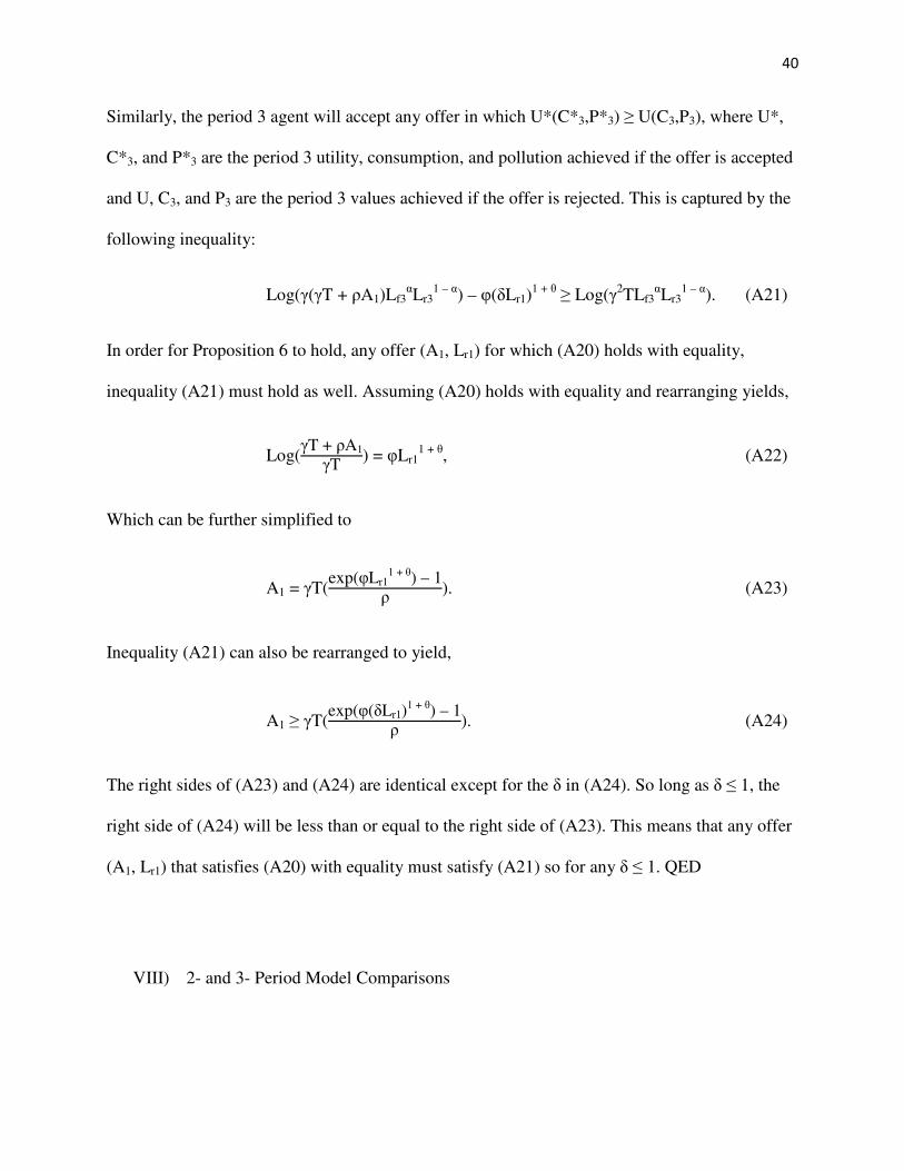
VII) Proof of Proposition 6

The period 2 agent will accept any offer in which U*(C*2,P*2) ≥ U(C2,P2), where U*, C*2, and

P*2 are the period 2 utility, consumption, and pollution achieved if the offer is accepted and U,

C2, and P2 are the period 2 values achieved if the offer is rejected. This is captured by the

following inequality:

Log((γT + ρA1)Lf2αLr2

1 – α) – φLr1

1 + θ ≥ Log(γTLf2

αLr2

1 – α). (A20)

0 0.5 1 1.5 2 2.51.7

1.8

1.9

2

2.1

2.2

2.3

2.4

2.5Rho Sensitivity Analysis Old SWF

Rho

We

lfare

Planner

Tax

Coase

Ind. Opt.

0 0.5 1 1.5 2 2.51.6

1.7

1.8

1.9

2

2.1

2.2

2.3Rho Sensitivity Analysis IA SWF

Rho

We

lfa

re

Planner

Tax

Coase

Ind. Opt.

0 0.5 1 1.5 21

1.2

1.4

1.6

1.8

2

2.2

2.4Theta Sensitivity Analysis Old SWF

Theta

Welf

are

Planner

Tax

Coase

Ind. Opt.

0 0.5 1 1.5 21

1.2

1.4

1.6

1.8

2Theta Sensitivity Analysis IA SWF

Theta

We

lfa

re

Planner

Tax

Coase

Ind. Opt.

40

Similarly, the period 3 agent will accept any offer in which U*(C*3,P*3) ≥ U(C3,P3), where U*,

C*3, and P*3 are the period 3 utility, consumption, and pollution achieved if the offer is accepted

and U, C3, and P3 are the period 3 values achieved if the offer is rejected. This is captured by the

following inequality:

Log(γ(γT + ρA1)Lf3αLr3

1 – α) – φ(δLr1)

1 + θ ≥ Log(γ

2TLf3

αLr3

1 – α). (A21)

In order for Proposition 6 to hold, any offer (A1, Lr1) for which (A20) holds with equality,

inequality (A21) must hold as well. Assuming (A20) holds with equality and rearranging yields,

Log(γT + ρA1

γT) = φLr1

1 + θ, (A22)

Which can be further simplified to

A1 = γT(exp(φLr1

1 + θ) – 1

ρ). (A23)

Inequality (A21) can also be rearranged to yield,

A1 ≥ γT(exp(φ(δLr1)

1 + θ) – 1

ρ). (A24)

The right sides of (A23) and (A24) are identical except for the δ in (A24). So long as δ ≤ 1, the

right side of (A24) will be less than or equal to the right side of (A23). This means that any offer

(A1, Lr1) that satisfies (A20) with equality must satisfy (A21) so for any δ ≤ 1. QED

VIII) 2- and 3- Period Model Comparisons

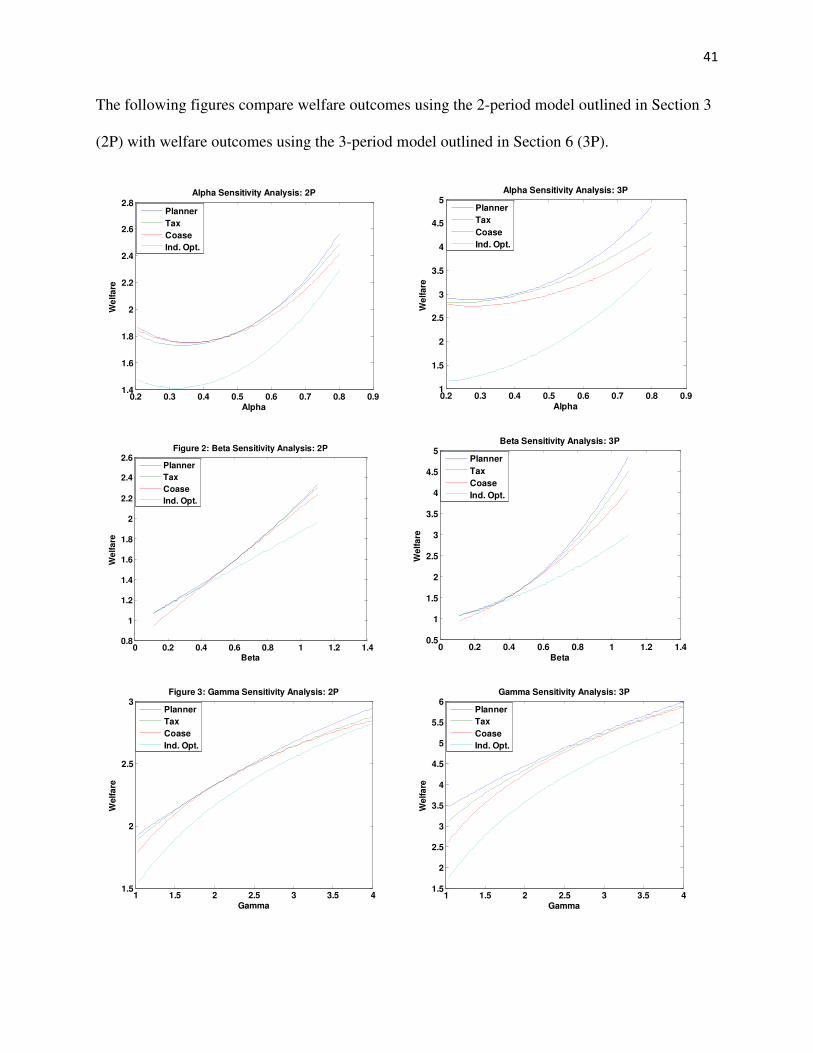
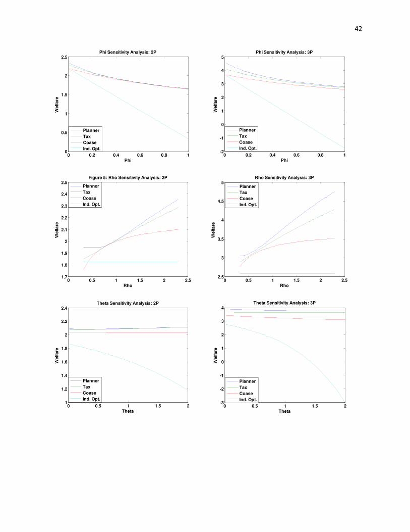
41

The following figures compare welfare outcomes using the 2-period model outlined in Section 3

(2P) with welfare outcomes using the 3-period model outlined in Section 6 (3P).

0.2 0.3 0.4 0.5 0.6 0.7 0.8 0.91.4

1.6

1.8

2

2.2

2.4

2.6

2.8Alpha Sensitivity Analysis: 2P

Alpha

We

lfa

re

Planner

Tax

Coase

Ind. Opt.

0.2 0.3 0.4 0.5 0.6 0.7 0.8 0.91

1.5

2

2.5

3

3.5

4

4.5

5Alpha Sensitivity Analysis: 3P

Alpha

We

lfa

re

Planner

Tax

Coase

Ind. Opt.

0 0.2 0.4 0.6 0.8 1 1.2 1.40.8

1

1.2

1.4

1.6

1.8

2

2.2

2.4

2.6Figure 2: Beta Sensitivity Analysis: 2P

Beta

We

lfa

re

Planner

Tax

Coase

Ind. Opt.

0 0.2 0.4 0.6 0.8 1 1.2 1.40.5

1

1.5

2

2.5

3

3.5

4

4.5

5Beta Sensitivity Analysis: 3P

Beta

We

lfa

re

Planner

Tax

Coase

Ind. Opt.

1 1.5 2 2.5 3 3.5 41.5

2

2.5

3Figure 3: Gamma Sensitivity Analysis: 2P

Gamma

Welf

are

Planner

Tax

Coase

Ind. Opt.

1 1.5 2 2.5 3 3.5 41.5

2

2.5

3

3.5

4

4.5

5

5.5

6Gamma Sensitivity Analysis: 3P

Gamma

We

lfa

re

Planner

Tax

Coase

Ind. Opt.

42

0 0.2 0.4 0.6 0.8 10

0.5

1

1.5

2

2.5Phi Sensitivity Analysis: 2P

Phi

Welf

are

Planner

Tax

Coase

Ind. Opt.

0 0.2 0.4 0.6 0.8 1-2

-1

0

1

2

3

4

5Phi Sensitivity Analysis: 3P

Phi

We

lfa

re

Planner

Tax

Coase

Ind. Opt.

0 0.5 1 1.5 2 2.51.7

1.8

1.9

2

2.1

2.2

2.3

2.4

2.5Figure 5: Rho Sensitivity Analysis: 2P

Rho

Welf

are

Planner

Tax

Coase

Ind. Opt.

0 0.5 1 1.5 2 2.52.5

3

3.5

4

4.5

5Rho Sensitivity Analysis: 3P

Rho

Welf

are

Planner

Tax

Coase

Ind. Opt.

0 0.5 1 1.5 21

1.2

1.4

1.6

1.8

2

2.2

2.4Theta Sensitivity Analysis: 2P

Theta

Welf

are

Planner

Tax

Coase

Ind. Opt.

0 0.5 1 1.5 2-3

-2

-1

0

1

2

3

4Theta Sensitivity Analysis: 3P

Theta

We

lfa

re

Planner

Tax

Coase

Ind. Opt.