2011 lab book v3

8/3/2019 2011 lab book V3

http://slidepdf.com/reader/full/2011-lab-book-v3 1/117

Lead lab 2011Monday, February 06, 2012

Exercise (Class) Calibrate Your Writing 2Reading/Reference: Sampling Methods 4

Soil Sampling (Chicago Department Public Health) 5House Dust Sampling (ASTME-1728-95) 7Vacuum Dust Sampling 9Water Sampling 10Blood Sampling 11Hand Dust Sampling 12Lead in Toys, Cosmetics, Glazes 13

Exercise (Lab) Sampling a Population of Potatoes 14Reading Statistics of Sampling and Measuring 26Exercise (Lab) Electronic Statistics and Measurements 42Reading/Reference: Extractions 53

Hot Plate Acid Digestion EPA 200.2 54Sequential Soil Extractions 56Microwave Digestion 58

Exercise: (Class) Lead by Spot Tests 56Exercise: (Lab) Lead by Dithizone Extraction and UV-Vis 60Exercise: (Lab) Lead by Calcein Blue and Fluorescence Quenching 70Exercise: (Lab) IR Determination of Pb binding to EDTA 76Exercise: (Lab) NMR and Lead 207 in EDTA 79Exercise: (???) Circular Dichroism and binding of lead to calmodulin 83Exercise(Lab) Lead ISE 84Exercise(Lab) Lead by ASV 97

Exercise:(Lab) Lead by Flame Atomic Absorption 102

1

8/3/2019 2011 lab book V3


1 Revised 2010

Calibrate Your Writing

This lab is a writing intensive lab where the work and writing are a collaborative process. Thecollaborative process requires certain documentation in order to be successful. The designationwriting intensive has specific requirements, one of which is that the student obtain feedback onhis/her writing and be required to revise their work based on the feedback.

In order to facilitate this collaborative writing intensive process we will begin by “A” reviewingadvantages/disadvantages of collaborative work and “B” “calibrating” what we consider to begood quality writing.

Procedure

A. Collaborations

1. Read the attached article on the value of collaborations in the commercial laboratory.

2. As an individual, list 3 benefits and 3 pitfalls of team work. For the 3 pitfalls, pick 1 andwrite a 1 paragraph protocol (series of steps, checks, benchmarks) that would minimizethat pitfall.

3. Gather into your group and share your list of 3 benefits and 3 pitfalls. Collectively prepare a report to be included in your writeup.

B. Calibrating the Quality of Your Writing

1. Each person in your group should Read the two lab reports entitled: “GFAA Group Aversion 1" and “version 2". Rank the two as “poor, good, excellent”.

2. Compare your rankings with the other members of your group. Do you agree? If youagree go to step 5.

3. If you do not agree each person should separately read the two lab reports entitled:“GFAA Group E version 1" and “version 2". Rank the two as “poor, good, excellent.”

4. Compare your rankings with other members of your group. Do you agree? If you do notagree consult with the “coach”.

5. Based on your ranking set up some specific numerical scale based on (but not limited tothe following criteria)

General: Grammar, spelling, paragraph lead sentence and follow up withinthe paragraph; lead into next paragraph, over all “flow” of the text

2

8/3/2019 2011 lab book V3


Scientific: Ease of readability of the tables and graphs; do you feel capable of reproducing the work with the material presented?

Clarity: Can you follow the objective of the students? Did they tell astory? Did they “milk the cow” in extracting all of the meaningfrom the data? Did they discuss the meaning of their graphs (or

conversely, did their graphs contribute to the flow of the story?)Lab Book Was their attached lab book data clear - would you be able to writea patent from it?

Group Work Did the students indicate who did what job in the lab clearly?

6. Using the numerical scale you have developed, apply that scale to the 3 lab reportsentitled “ICPMS Group B” “C” and “D”

1Appendix Article: Teamwork, C&EN, Nov. 15, 1999

Series of previous lab reports to be read and calibrated

3

8/3/2019 2011 lab book V3


Sampling

MethodsSoil samplingDust Sampling with Wet WipesDust Sampling by VacuumWater SamplingBlood SamplingHand Dust SamplingLead in Toys

Lead in Cosmetics1Lead in Glazes

4

8/3/2019 2011 lab book V3


1 Soil Sampling

SYNOPSIS: A soil sample procedure recommended by the Chicago

Department of Health is followed. The sampling is designed tocover the largest area as well as the areas most likely to deviatein soil lead content. The sampling is also designed to createrepresentative samples at any one given site.

PROCEDURE:

Make an area map with buildings and boundaries (sidewalks, driveways, etc.)See next page.

1. Sample two feet from building every 10 feet along the side.2. Wipe a plastic spoon with a tissue and dig a 1 inch diameter andno more than 1 inch deep sample. Combine all samples along agiven side of the building into a sealable plastic bag and label.(Date, Building, map location, student)

3. Sample play areas separately (in 10 ft intervals). Each sample iskept separate in own bag and labeled according to position onmap, student, date.

REPORT In addition to materials, methods, and results, your report shouldinclude:

1. How were your samples randomized?2. What efforts were taken to avoid contaminating the sample?3. How were the samples labeled in order to achieve good quality

control?4. In soil sampling, what effect will the depth of sampling have on

your sample (see Chapter 10, gasoline dispersion of lead)?5. How was the sample stabilized to prevent losses in transit and

storage? Be specific for the type of sample you have.6. Attach a neatly drawn map of your sampling and attach it to your

report.

8/3/2019 2011 lab book V3


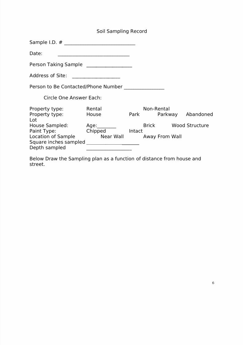
Soil Sampling Record

Sample I.D. # ______________________________

Date: ______________________________

Person Taking Sample ___________________

Address of Site: ____________________

Person to Be Contacted/Phone Number _________________

Circle One Answer Each:

Property type: Rental Non-RentalProperty type: House Park Parkway Abandoned

LotHouse Sampled: Age:________ Brick Wood StructurePaint Type: Chipped IntactLocation of Sample Near Wall Away From WallSquare inches sampled ______________________ Depth sampled ___________________

Below Draw the Sampling plan as a function of distance from house andstreet.

6

8/3/2019 2011 lab book V3


House Dust Sampling

SYNOPSIS A sampling procedure for house dust is used that is extractedfrom various housing authorities and from ASTM E-1728-95

INTRODUCTION Two types of sampling procedures are used for house dust. Theseinclude wet wiping and vacuuming with a high velocity vacuum. Thelatter is becoming standard, however wet wiping can be convenient forowner/occupant sampling. When wet sampling is used the key is toprovide an adequate control (un-used wipe). In general therelationship between wet wiping and vacuum sampling is linear, withthe lead measured from wet wipes generally being higher thanmeasured from vacuuming. It is presumed that the higher level of leadis biased for the wet wipe procedure.

PROCEDURE

1. Make a number of disposable 1 ft square (i.d.) templates fromcardboard. The number should equal the number of samples to beobtained.

2. Draw a map of the house floor plan.3. Select a room, one which is most likely to be occupied by children

(living room or bed room). Draw a floor plan for the room.4. Put on powderless gloves. Powder can cause false positives for lead.5. Open box of wipes. Through away three to remove any contamination

due to opening of the box.6. Remove one wipe and place in a clean baggie and Label it with your

name, the date, the house, the room, and title it "control #1".7. You should plan collecting a control for every 10 samples. When you

are down you should have a minimum of three controls (in separatebaggies) and a control sampling rate of 5%..

8. Sample at the door and/or in the window sill and/or below the windowsill.

9. Lay down the template, taping the outer edges in place. Remove onewipe and with gentle pressure wipe the entire surface inside thetemplate clean, using an S motion.

10. Transfer the sample to a clean baggie and label it with your name, thedate, the house, the room, the location sampled in the room, and titleit with the location.

11. After 10 samples, set aside in a clean baggie and labeled as above,another control.

7

8/3/2019 2011 lab book V3


REPORT In addition to materials, methods, and results, your report shouldinclude the following information:

1. How were your samples randomized?2. What efforts were taken to avoid contaminating the sample?

3. How were the samples labeled in order to achieve good qualitycontrol?4. How was the sample stabilized to prevent losses in transit and

storage? Be specific for the type of sample you have.5. Why is the total size sampled important? Why are the common areas

for sampling near windows and/or doors?6. Attach a neatly drawn map of your sampling and attach it to your

report.

Hust Dust Sampling Record

Sample I.D. # ______________________________

Date: ______________________________

Person Taking Sample ___________________

Baby Wipe Lot Number ____________________________

Address of Housing Unit: ____________________

Person to Be Contacted/Phone Number _________________

Circle One Answer Each:

Property type: Rental Non-RentalRoom sampled Living Room Kitchen Child'sBedroomSample type: Surface Washed Surface Un-usedWipePaint Type: Chipped IntactLocation of Sample Window Sill Floor near window floor

near doorSquare inches sampled ______________________

Below Draw the Floor Plan of the Room.

8

8/3/2019 2011 lab book V3


9

8/3/2019 2011 lab book V3


Vacuum Dust Sampling

SYNOPSIS: Dust is sampled using a filter and vacuum. The advantage of this method is a smaller amount of material to be digested.

Materials:Personal air sampling pump (an aquarium pump may serve)0.8 μm pore size, 37-mm diameter cellulose ester filterfilter holdertweezerstubing 0.60 cm inside diameterpowderless glovessoap bubble calibration devicetape

Method

1. In the lab calibrate the air flow by the pump with a soap bubble (seenext page). The flow rate should be 1-5 L/min calibrated to 5%.

2. Keep note of the calibration of the pump within the lab book.3. Put on the powderless gloves4. Assemble the collection filter device, consisting of the filter holder and

filter paper. Seal the filter holder with plastic tape and label.5. Attach the 0.60 tubing to the top of the filter capsule. The end of the

tubing should be cut to a 45 angle.

6. Attach the 0.60 cm i.d. tubing to the bottom of the filter capsule and tothe pump. The distance should be greater than 5, but less than 10 cm.

7. Place the template (1 ft square i.d. disposable cardboard) on thesurface and tape down.8. Move the Nozzle across the surface (in contact but without pressure)

with the 45 cut flat on the surface at a rate of 10 to 20 cm/s. Vacuumentire surface in a side to side motion.

9. Repeat but at a 90 degree angle from the first vacuuming.10. Repeat at the original direction.

10

8/3/2019 2011 lab book V3


Water Sampling

SYNPOSIS Sample procedures for obtaining tap water are given. Themethod used is that recommended by the Water Works

Association .

PROCEDURE

1. Take first morning cold water sample from kitchen tap: Let coldwater run 30 s. Rinse plastic bottle several times. Fill to neckand cap.

2. Let cold water run for 1 minute and take a second labeledsample.

3. Let cold water run for 5 minutes and take a third labeled sample.4. Acidify each sample to pH 1.5 or 2 with concentrated HCl.

REPORT In addition to materials, methods, and results, your report shouldinclude the following information:


control?4. How was the sample stabilized to prevent losses in transit and

storage? Be specific for the type of sample you have.5. Attach a neatly drawn map of your sampling and attach it to your

report.

11

8/3/2019 2011 lab book V3


Blood Sampling

SYNOPSIS Blood samples are taken for measurement of lead. The methodused was that recommended by the CDC in 1991.

MaterialSoapAlcohol swabsSterile cotton ballsSilicone spray or swabsExamination gloves (powderless)Capillary fingerprick (Drummond Sci.)Bandages

PROCEDURE

1. Rinse gloves to remove powder and put on.2. Wash the childs hands with soap and dry.3. Use the middle finger and check that it has no visible infection orwound.4. Massage the finger to increase blood circulation.5. Grasp the finger between the thumb and index finger with the palm of

the child’s hand up.6. Clean the ball or pad of the finger with alcohol swab. Dry with sterile

cotton ball.

7. Apply the silicone barrier.8. Puncture with the capillary fingerprick - using potassium EDTA treated

wiretol micropipettes (Drummond Sci.).9. To get blood flowing massage finger gently.10. Seal one end with Critoseal (Thomas Co. Phil, Pa.) cap and one end a

critocap.11. Store < 8 weeks at 8oC or 10 days at ambient temp.12. Stop bleeding and cover fingertip with bandaid.

REPORT In addition to materials, methods, and results, your report should

include the following information:


control?

12

8/3/2019 2011 lab book V3


4. How was the sample stabilized to prevent losses in transit andstorage? Be specific for the type of sample you have.

13

8/3/2019 2011 lab book V3


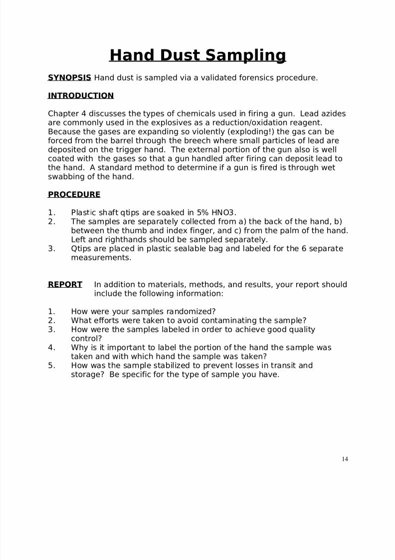
Hand Dust Sampling

SYNOPSIS Hand dust is sampled via a validated forensics procedure.

INTRODUCTION

Chapter 4 discusses the types of chemicals used in firing a gun. Lead azidesare commonly used in the explosives as a reduction/oxidation reagent.Because the gases are expanding so violently (exploding!) the gas can beforced from the barrel through the breech where small particles of lead aredeposited on the trigger hand. The external portion of the gun also is wellcoated with the gases so that a gun handled after firing can deposit lead tothe hand. A standard method to determine if a gun is fired is through wetswabbing of the hand.

PROCEDURE

1. Plastic shaft qtips are soaked in 5% HNO3.2. The samples are separately collected from a) the back of the hand, b)

between the thumb and index finger, and c) from the palm of the hand.Left and righthands should be sampled separately.

3. Qtips are placed in plastic sealable bag and labeled for the 6 separatemeasurements.

REPORT In addition to materials, methods, and results, your report should

include the following information:


control?4. Why is it important to label the portion of the hand the sample was

taken and with which hand the sample was taken?5. How was the sample stabilized to prevent losses in transit and

storage? Be specific for the type of sample you have.

14

8/3/2019 2011 lab book V3


Lead In ToysHenry Browner: Screening Testing for Lead and Cadmium in Toys and Other Materials Using AAS

Journal of Chemical Educatio, 82, 4, 2005, 611

Consumer Products Safety Commission: CPSC-CH-E1002-08: Standard Operating Procedures forDetermination of Total Lead in non-metal children’s produces, Feb. 1, 2009

CPSC-CH-E1001-08 Standard Operating Procedures for Determining total lead in Children’s MetalProducts Dec. 4, 2008

Lead in Cosmetics

Lead in GlazesLead in Glazes: ASTM C 103Lead in Glazes: ASTM C1035 Jarcho, Saul, American Antiquity, 30, 1, 1964, Lead in the Bones of Pre-historic Lead-Glaze PottersA Meiklejohn. British Journal of Industrial Medicine, 1963, 20, 169, The Successful Prevention of LeadPoisoning in the Glazing of Earthenware in the North Staffordshire Potteries.

15

8/3/2019 2011 lab book V3


Revised 20101

Statistics Analyzed on SpreadSheets

SYNOPSISStudents have an introduction of lab recording, reporting, determination of standard deviations associated with random error, use of Excel. Read theNew England Journal of Medicine( http://www.luc.edu/faculty/afitch/Articles/Needleman%20NEJM%201979.pdf ) Needleman article and “Introduction to Statistics and Sampling” beforecoming to lab.

INTRODUCTIONIn this experiment students will collect data from two or more visibly

different populations. The random spread of the populations as a function of sampling size will be followed on a spread sheet as a histogram. Theresolution between the populations will also be followed. In addition,students will compute the standard deviation of the populations and followthe magnitude of the standard deviation as a function of population size.Finally, students will determine, by ANOVA (analysis of variance), if the twopopulations are statistically (significantly) different.

Testable SKILL OUTCOMES1. Review and/or learn basic spreadsheets “tricks” (see end of

document) (copy, paste, highlight, keyboard shortcuts)2. Review and/or learn basic spreadsheet calculations for standarddeviation, average, searching minimum, maximum, histogramand ANOVA functions

3. Review and/or learn graphing in a spreadsheet.4. Quality Control – multiple operators, random sampling as sources

of error.5. Learn how to create Gaussian curves and understand how the

parameters of a normal population allow us to maximize thequality of our measurements

6. Understand qualitatively and quantitatively how to place a

numerical value on certainty.

READING: “Introduction to Statistics and Sampling” posted on the Lead labweb page.

MATERIALS Several sacks of red and white potatoes.

16

http://www.luc.edu/faculty/afitch/Articles/Needleman%20NEJM%201979.pdf

http://www.luc.edu/faculty/afitch/Articles/Statistics.pdf

http://www.luc.edu/faculty/afitch/Articles/Needleman%20NEJM%201979.pdf

http://www.luc.edu/faculty/afitch/Articles/Statistics.pdf

8/3/2019 2011 lab book V3


SCENARIO A potato farmer has arrived in town with several sample sacksof sorted potatoes to show to potential grocers to demonstrate quality. Inaddition the farmer had several truck loads of potatoes to sell, however thetrucks were over turned so all the non-sample product were jumbled. Your job is to use the sample sacks to create a method to re-sort the potatoes.

You need to be able when done (using an ANOVA) to assure the grocers theprobable impurity of the resorted potatoes. The farmer is employing familymembers to help in the resorting process, all of whom are color blind.Furthermore, the farmer is cheap and will not purchase any equipmentbeyond strings and rulers to help in the sorting.

PROCEDURE

a. Break into several groups of 2 students each. Name your groups witha unique identifier. Divide each type of potato proportionally betweengroups.

b. Create a method to analyze within the lab the red and white potatoeswithout using color. The method must be numerical.1 The method mustinclude quality control measures which identify various sources of error and measures or accounts for those errors. The errors may stemfrom instruments used or from the operator. The method must also takeinto account a pre-determined procedure for obtaining a representativesubset of the population for measurement.

c. Confer with other groups and discuss your method. Choose a methodwhich all groups will use that appears to be the most efficient and

which has the best quality control. Begin measurements.

d. Transcribe your data into Excel spreadsheet as a series 4 columns. Thefirst column should be the number of potatoes measured from 1 to N. The second column should be the measurement you have chosen inyour method. The third column will identify the group from which thedata is obtained. This is most easily accomplished if one student readsout the data to another who is recording the data. To facilitategraphing and other Excel manipulations leave a blank row at the topand bottom of your column of data.

1 Instructor: bring strings, rulers, scissors, bucket of water if you wish. Students willnormally choose to do the circumference. The best result is obtained when using the longaxis for circumference. Students should be asked what source of error will occur in themethod and how to create a greater throughput. I.E. if each student samples then there willbe variability from student to student. A good method is to ask students to measure thesame potato 4 times and chose the student with the least standard deviation. to make themeasurement).

17

8/3/2019 2011 lab book V3


In the image above empty rows are highlighted.

e. Do not sort your data. Exchange data with other groups, keeping track of measurements deriving from other groups, by placing the group unique identifier in thefourth column.

1. Create a Frequency Plot of your first set of potatoes (your unique groups set of data)

ii. Determine the largest and smallest measurements made. At the end of the

measurement column type in the formula:=min(data set)

To highlight the data set right click on the first measurement, then holddown CNTRL, SHIFT, ↓ (the down arrow simultaneously). (Note thiscommand will highlight all the data until it reaches an empty row, which iswhy we left a blank row at the end of a given set of data).

In the next row find the largest measurement for that type of potato bytyping in the formula:

=max(data set)

Highlight the data set by holding down CNTRL, SHIFT, ↓

Copy your formulas left to right across your various data sets.Highlight the two formulas, then using the keyboard ALT, E, C. The“Alt” command allows you to access the command tab at the top of the page. “E” indicates that you wish to open the “edit” tab, and the“C” indicates that you wish to use the “copy” command. To copy you

18

8/3/2019 2011 lab book V3


can play the cursor on the lower right box that appears in thehighlighted cells and drag to the right.

iii. Create “bins”. You are familiar with this process when an instructorshows the distribution of grades in a class in which the number of

students getting an exam score is plotted on the y axis vs the grade“bin”. The range of the grade bins is from the minimum grade to themaximum grade or from 0 to 100%. The bin width for the grades isvariable (90-91% vs 90-95% vs 90-100%).

Your range of bins for your measurements should be fromslightly smaller than your smallest number to slightly larger than yourlargest number from all classes of potatoes as you will be plottingmultiple sets of data in a single graph. The bin width will affect thegraph you ultimately get. You want neither too large of bin (all gradesbetween 0-100%) nor too small (sorting grades by 0.5%).

Create a column for your bins. In the first cell type the value of the lowest bin, ENTER. Return to the value and highlight it. Create thebins by typing ALT, E, I, S. This will open a command box labeledseries. Type ALT, C to indicate your bins will be in a column ratherthan in a row. Type ALT, S to highlight the step box. This determinesvalue you increment (bin width). Type ALT, O to highlight the stop box.Enter the maximum value for the range of bins. ENTER to create thecolumn of bins.

iv. Sort your data into bins. ALT, T, D, D, ENTER, then ↑or ↓ to “Histogram”,

and then ENTER which opens a command box “Histogram” in whichthe cursor is in the Input Range box. Either type in the range of yourdata (for example A1:A20) and then type ALT I to access the bin range.Or: click on the Excel sheet icon at the right of the command line andthen highlight the data range; click on the Excel icon again to re-enterthe command box. Type ALT I to access the bin command line. Usinga similar procedure enter the bin range. Type ALT O to highlight thecommand line which specifies where the sorted data is to be placed.Place the cursor in the command line and then specify by typing in acell address or by using the icon to move to the cell address. ENTER toget your sorted data.

In order to facilitate graphing you need to create an empty row aboveand below the sorted data. Do not include the label row and do notinclude the “more” row.

v. Create the Frequency Plot. Highlight the bins (x value) and the sorteddata (y value). ALT, I, H to activate the chart commands. ALT, C and ↑

19

8/3/2019 2011 lab book V3


or ↓ to XY scatter. ALT, T to activate the subtypes. ↑or ↓ to eitherpoints, or points with straight lines. (NEVER use the curved lines asthis indicates that you have some knowledge of the mathematicsrelating the value of y to x). ALT, N to enter the commands for theplot.

20

8/3/2019 2011 lab book V3


2. Create a Gaussian Curve associated with your Histogram.

i. Calculate the standard deviation of the population of potatoes. Goto the bottom of the column of data (below your minimum andmaximum calculations) and type

=stdev(cell range)

Again you can highlight the cell range by activating the last or first cellin the range and then CNTRL SHIFT ↑or ↓.

ii. Name the cell containing the stdev. To name this cell highlight thecell. You should see a small box just above the cell ranges and belowthe command bar that displays the address of the cell you havehighlighted. Click and the address will go gray. Backspace to erase. Type in a unique name for this cell. Remember you will be making

several calculations of standard deviation for different size populationsof the same potato group and for different types of populations so you

should choose a name like stdevredall for a standard deviation of all of the red potatoes.

21

8/3/2019 2011 lab book V3


iii. Calculate the average of the population of potatoes. In the next rowtype

=average(cell range)

Name this cell so that you can refer to it when writing formulas.

iv. Calculate the predicted frequency or Gaussian. A perfectly randompopulation should have a frequency plot described by the equation:

2

2

1

exp2

1

−

−

= σ

µ

π σ

x

y (1)

Where y is the probability of finding a particular measurement betweenx and dx (the bin width) when the average is x and the standard deviationis σ . For a normalized population the area under the curve is 1 and thepeak height is 0.33. To match our data we need to scale the Gaussian by theexpected peak height for our population value (N) distributed over x-dx (binsize).

)(dx N A =2

2

1

exp2

−

−

= σ

µ

π σ

x A

y

Create a cell with the value of “A” and name it as “peakheight”

Move your cursor to an empty column and to the same row as yourfirst (lowest numerical value) bin. Type in Equation 1 using Excellanguage as:

=(peakheight/(stderedall *sqrt(2*pi()))*(exp(-0.5*((bin-averedall )/stdevredall )^2)

In this equation where it says bin, highlight the “bin” for the row youare in. Stderedall refers to the cell in which you have calculated thestandard deviation using all of the red potatoes. Averedall refers tothe cell in which you calculated the average using all of the red

22

8/3/2019 2011 lab book V3


potatoes. peakheight refers the value “total measurements xbinwidth)

(Another way to always refer to a unique cell is to insert $ into the celladdress. A $ before the column ($A1, for example) indicates that Excel

should always refer to column A when copying the formula, yet allowsthe row to move down as the formula is copied down. A $ before therow (A$1) indicates that Excel should always refer to row 1 whencopying the formula but allow the column to move as the formula iscopied to the right or left. If the cell is referred to as ($A$1) when theformula is copies it will always refer to cell A1.)

Copy your formula down so that each “bin” has a projected frequencyvalue.

iv. Add the expected value to the histogram plot. Highlight the top

or bottom cell of the calculated, predicted, frequencies andsimultaneously press CNTRL SHIFT ↑or ↓ to highlight yourcalculated values. ALT, E, C to activate the cells. Then go toyour plot page. ALT, E, paste.

To insert a set of data into your graph that has different X valuesuse paste special and indicate that the first column containsthe x values.

3. Calculate the estimated width of your Gaussian by taking thederivative of the Gaussian.

i. Insert 2 columns adjacent to your calculated (theoretical)frequency values.

ii. The first column will be the mid bin value. If, for example the cellcontaining the first bin is Q10, in row 10 of your column type

=Q10+(Q11-Q10)/2

iii. Copy this formula down to the N-1 bin rowiv. The second column will contain the derivative of the frequency (y

axis). If the computed frequency begins in cell R10, in row 10 of your second column type

=(R11-R10)/(Q11-Q10)

v. Plot the first column as x and the second column as y in thesame graph as your theoretical frequency.

23

8/3/2019 2011 lab book V3


vi. Calculate the standard deviation by taking the max and min of your just calculated derivative data. Calculate the differencebetween the x location of the max and the x location at zero. Dothe same for the min. The two values should be similar and

should be similar to your calculated standard devition in 2.iii above.

Describe verbally the shape of your derivative curve withrespect to the raw data curve.

4. Repeat 1&2

i. Repeat the analysis for increasing population of measurements byincluding data for this kind of pototo from other groups. Be sure toget a mean and average deviation for each group’s sample of measurements so that you can discuss the effect of multipleoperators in your data analysis.

j. Repeat the analysis for the different kinds of potatoes.

k. Copy (without sorting) all of the data into one large population of measurements and repeat 1 & 2.

5. Difference between Experimental Histogram and Model Gaussian

One way to test if your model Gaussian is “good” is to calculatethe absolute difference between the Gaussian and theexperimental histogram at every point and sum. A convenientway to get an absolute value is to square.

i. In a new column in the same row as the first bin number type the

Excel formula: =(histogram value-model value)^2ii. Copy this down to the end of the bin numbers.iii. Sum this column of data. This represents the sum of squares.iv. Repeat for different populations. What happens to the sum of

squares for different size populations?

6. Calculate the Resolution of your red and potato populations

Resolution refers to how well separated your histograms are. Resolution iscalculated as:

(

+

−=

22

ba

ab

W W

x x R

24

8/3/2019 2011 lab book V3


where i x refers to the mean of population I and Wi refers to the baseline

width of peak i. The baseline width can be obtained by triangulating thepeak.7. Calculate the Analysis of Variance of your red and potatopopulations

i. You will need to have the raw data for your red and white potatopopulations in adjacent columns. Copy and move your data to someconvenient location.

ii. ALT, T, D, D, ENTER. Use the arrow key to move to ANOVA, singlefactor. ENTER. The command box for the ANOVA is now displayed. Highlightboth columns of data for the input range.

iii. If you wish to test that you can be 95% certain that there are twodifferent populations set the alpha factor to 0.05. If you wish to test that you

can be 99% certain that there are two different set the alpha factor to 0.01.

iv. Activate the output range and set it to some convenient location.ENTER.

v. If the calculated F value is greater than the F critical value then youare alpha confident that you have two different populations of potatos.

8. Compute a running averages and running standard deviations.2

i. A running value is one that is calculated with an ever increasingpopulation. That is, for two points compute the average and standarddeviation of two points. For three points compute the average of threepoints and the standard deviation of those three points.

Place your cursor in an empty column in the row of your first datapoint. For example if your first measurement for red potatoes is in cella10 place your cursor in some column, row 10. Type in the followingformula:

=average(A10:A$10)

2 Instructor: At this point it is very important that the sampling have been random as well as having a random population of potatoes. If the sampling procedure was random then the standard deviation will decrease as thesquare of the number of measurements made. If the sampling was not random, the plot will not demonstrate this point.

25

8/3/2019 2011 lab book V3


Copy this formula down the column to the last row of data. You shouldsee that the formula starts by calculating the average of A10:A10; thenA11:A10; then A12:A10; and so on.

ii. Repeat this process for a running standard deviation:

=stdev(A10:A$10)

iii. Make a plot of the average circumference and standard deviation as afunction of sample number.

26

8/3/2019 2011 lab book V3


9. Analyze the Needleman Data. You can obtain the Needleman data in an Excel sheet form the Lead Lab web page.

This data was abstracted from the NIH report ORI 91-27.Data is reported as a percent of the total, where the total is N. The ORIreport investigated several allegations of scientific misconduct broughtagainst Needleman. One of these charges was that the selection of childrenas part of the low lead cohort (<6 ppm tooth lead) and of the high leadcohort (>24 ppm tooth lead) was misleading as the selection criteriachanged. A second charge was that the data was amended between 1979and 1982 in such a way as to imply that high tooth lead affected Verbal IQsin a uniform fashion. The ORI report stated: (p. 33) “According to theHearing Board, the preponderance of evidence indicated that Dr. Needlemandeliberately misrepresented the subject inclusion/exclusion procedures in his

original and subsequent publications. The Board speculated that thismisrepresentation may have been done to make the subjectinclusion/exclusion procedures appear much more rigorous than they were. The Board determined that this violates a principle of scientific inquiry,namely that procedures be described so that the observations could bereplicated by other investigators (Hearing Board Report, pages 39 and 64).Later in the ORI report (p. 75): As alleged by the complainants, the DRIanalysis shows that the graphs presented do not explicitly deal with thepossible effects of covariates such as age. The DRI analysis indicates thatthe 1982 Note contains errors, inconsistencies and misleading statementswhose combined impact is to favor a “simple shift” lead effect throughout

the entire VIQ range. The correction and clarification of the points raisedabove would serve scientific interests as well as, potentially, those of publicpolicy.

i. Use the data to construct frequency plots of the 1978comparison between the verbal IQ of children with high toothlead and children with low tooth lead.

ii. Use the data to construct frequency plots of the 1982 amendedset of data as compared to the 1978 data for the low tooth leadchildren..

http://www.luc.edu/faculty/afitch/Lead%20Lab.htm

http://www.luc.edu/faculty/afitch/Lead%20Lab.htm

8/3/2019 2011 lab book V3


REPORT Your report should have

A. A meaningful or descriptive title. (Neither Red and White Potatoes, nor First Lab aredescriptive titles).

B. A marked section (I) for the introduction or purpose.

C. A marked section (II) for materials and methods.

This section includes reagents used and their manufacturers and dilutions used inthe lab. If there are any changes in what is used or how much of a reagent is used,it should be noted here. Additionally, all instrumentation, including manufacturer and model number, any variable used and the settings for the lab should be noted.If reagents were made by the students, all calculations involving dilutions etcshould be included.

D. A marked section (III) for results in which graphs and tables are presented. Graphs are

both numbered and given a title. Graphs follow within the report immediately after thefirst time they are mentioned, and should be in numerical sequence.

E. A marked section (IV) for summary/discussion. Your lab report willbe marked down in grade if your summary/discussion section is simplya list of answers to the following questions. These questions are to beused as starting points or ideas.

1. In what ways does the quality of your data change when youincrease the number of samples measured? Give both graphs

and verbal descriptions of the graphs and numerical valueswhich describe the quality of the data?2. How well can you resolve the two types of potatoes? Does the

resolution change with increased sample size?3. Did your measurement protocol adequately account for all types

of possible sources of variation in the measurements?4. For the Needleman data

a. What has happened to the data between 1979 and 1982?

b. From the data estimate the Resolution between the verbalIQ of children with high and low lead. Why mightpublic policy be based on different standards for R than

analytical chemistry? What might be the consequenceof failure to act?5. If you were to re-do this laboratory would you change your

“protocol”? Explain your answer.

8/3/2019 2011 lab book V3


EXCEL TIP SHEET

Π is written as pi()Times *Divide /

Square root sqrt(number here)Standard deviation stdev(cell range)Average average(cell range)Mininium minimum(cell range)Maximum maximum(cell range)Exp exp(number here)

Making a copied equation refer always to a unique cell (for example A10):$A10 always refer to column A when copying the formula. When copying

down or up the row will will change proportionally.A$10 always refer to row 10. When copying left or right the column will

change proportionally.$A$10 cell A10 will always be referred to even when copying the formula updown or left and right.

ALT – will allow you to reach the command line at the two of the sheet by thekeyboard instead of using the mouse. If you get in the habit of doing thisyou will save literally hours of time. Follow with the indicated underlinedletter for the tab of the command line.

To highlight a column (or row) of data to copy or alter or paste the easiest way toavoid endless mouse scrolling is to make certain that your data is always

bookended by an empty row at the top and bottom (or left and right).Highlight the cell at the top (or bottom) of the column to be copied thensimulataneously press the CNTRL SHIFT and arrow key to get all the datahighlighted.

To fill a column with a set of numbers. Type in the first number you want in the desired cell;Enter. Then arrow up to highlight the cell. ALT, E, I, S. This will open a commandbox labeled series. Type ALT, C to indicate you want to create thenumber series in a column rather than in a row. Type ALT, S tohighlight the step box. This determines value you increment. TypeALT, O to highlight the stop box. Enter the maximum value for the

range of numbers. ENTER to create the column of numbers.

8/3/2019 2011 lab book V3


(Reading) 1Statistics of Measurements

A measurement can be considered to be an average of a small sample

from a population of an infinite series of measurements (a population) whichare influenced by the measurement process in random and non-randomfashions. Thus one's "true" weight may be at 145 lbs but wishful thinkingand a squinting eye (determinate error) sets the weight at 140 lbs. If oneweighs oneself everyday (Figure 1) for one year, a plot of those dailymeasurements will show some fluctuation about the "true" value. Ahistogram is also a measure of the fluctuation (Figure 5). The histogramrepresents a Gaussian or normal population that has not been sampledadequately. A “normal” curve is described by the function:

( )

2

121

exp2

x x

f xσ

σ π

−−

=

t

1where f(x) is the probability of observing the number (number of observations expected), σ is the variance which is estimated by thestandard deviation, s, x is the value of x and x is the mean value of x.Physicists and mathematicians refer to this as the zeroth moment. Thenormal error curve is shown in Figure 2.

Table Statistical MomentsMoment Function Common

nameformula

0 F(x) Probability( )

21

21 exp2

x

f x

µ

σ

σ π

−

− =

1 x Mean oraverage ( ) x f x dx µ

∞

−∞

= ∫ 2 x Standard

deviation ( )2 2 x f x dxσ µ ∞

−∞

= −

∫

3 skew shape( )3 2 2 skew x f x dx µσ µ

∞

−∞

= + +

∫

1 This curve has the following characteristics:

8/3/2019 2011 lab book V3


a. There is a peak at x = ìb. The peak is symmetric

c. 1 There are inflection points on either side of the peak whichdefine σ, which accounts for 68.3% of the measurements.

The first and second derivatives of the error curve are also shown. Thefirst derivative crosses the x axis at the mean of the population. The mean isthe first moment of the population and can be calculated by equation 2:

Figure 1 My weight over summer plotted as a function of pounds vs days. The first 11 days represent average

summer weight (baseline). The next 10 days represent weight gain during vacation, and the final section

represents weight gain on the beginning of the semester. The line marked peak to peak variation represents the

maximum and minimum weights measured during the beginning of the school year.

Figure 1 My weight over summer plotted as a function of pounds vs days. The first 11 days represent average

summer weight (baseline). The next 10 days represent weight gain during vacation, and the final section

represents weight gain on the beginning of the semester. The line marked peak to peak variation represents the

maximum and minimum weights measured during the beginning of the school year.

31

8/3/2019 2011 lab book V3


Figure 1 The standard (s=1, μ=0) error curve, with its first and second derivatives showing that the curve

has inflection points at s ± 1. The inflection points are observed in the first derivative as the points at

which the curve crosses the x axis and in the second derivative as peaks.

Figure 1 The standard (s=1, μ=0) error curve, with its first and second derivatives showing that the curve

has inflection points at s ± 1. The inflection points are observed in the first derivative as the points at

which the curve crosses the x axis and in the second derivative as peaks.

igure1 Histogramorfrequencyplot of theweight datafromabovefigureforthe“baseline”and“vacation” portionsof thedata. Thestripedareasrepresent thefit normal curvetothedata(solid) basedonthecalculated meanandstandarddeviations. Notethat the“real”dataisnot well approximatedbythenormal datawiththis

populationsize, andthat theestimatedpopulations signficantly overlap.

32

8/3/2019 2011 lab book V3


Figure 1 A Normal or Gaussian or error curve for samples of an N-1,000,000 member

true population with a population standard deviation of 1. The sample size, n, increases

from 3, 6, 9, 10, 15, 20, 25, 30, 50, to 75. As the sample size increases the standard

deviation of the sample decreases while the peak associated with the mean increases .

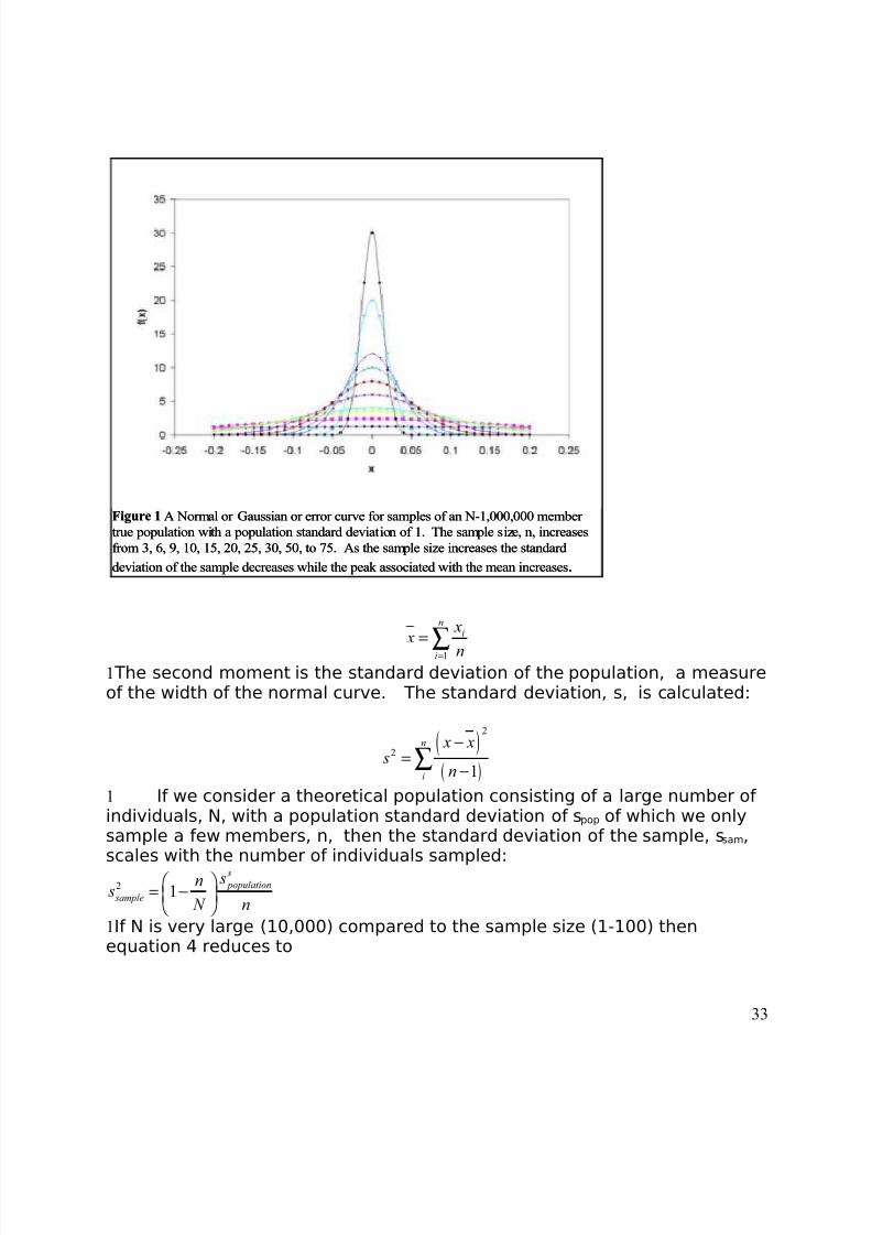
Figure 1 A Normal or Gaussian or error curve for samples of an N-1,000,000 member

true population with a population standard deviation of 1. The sample size, n, increases

from 3, 6, 9, 10, 15, 20, 25, 30, 50, to 75. As the sample size increases the standard

deviation of the sample decreases while the peak associated with the mean increases .

1

ni

i

x x

n=

=

∑1 The second moment is the standard deviation of the population, a measureof the width of the normal curve. The standard deviation, s, is calculated:

( )( )

2

2

1

n

i

x x s

n

−=

−∑1 If we consider a theoretical population consisting of a large number of individuals, N, with a population standard deviation of spop of which we onlysample a few members, n, then the standard deviation of the sample, ssam,scales with the number of individuals sampled:

2 1

s

population

sample

sn s

N n

= −

1If N is very large (10,000) compared to the sample size (1-100) thenequation 4 reduces to

33

8/3/2019 2011 lab book V3


population

sample

sample

s s

n=

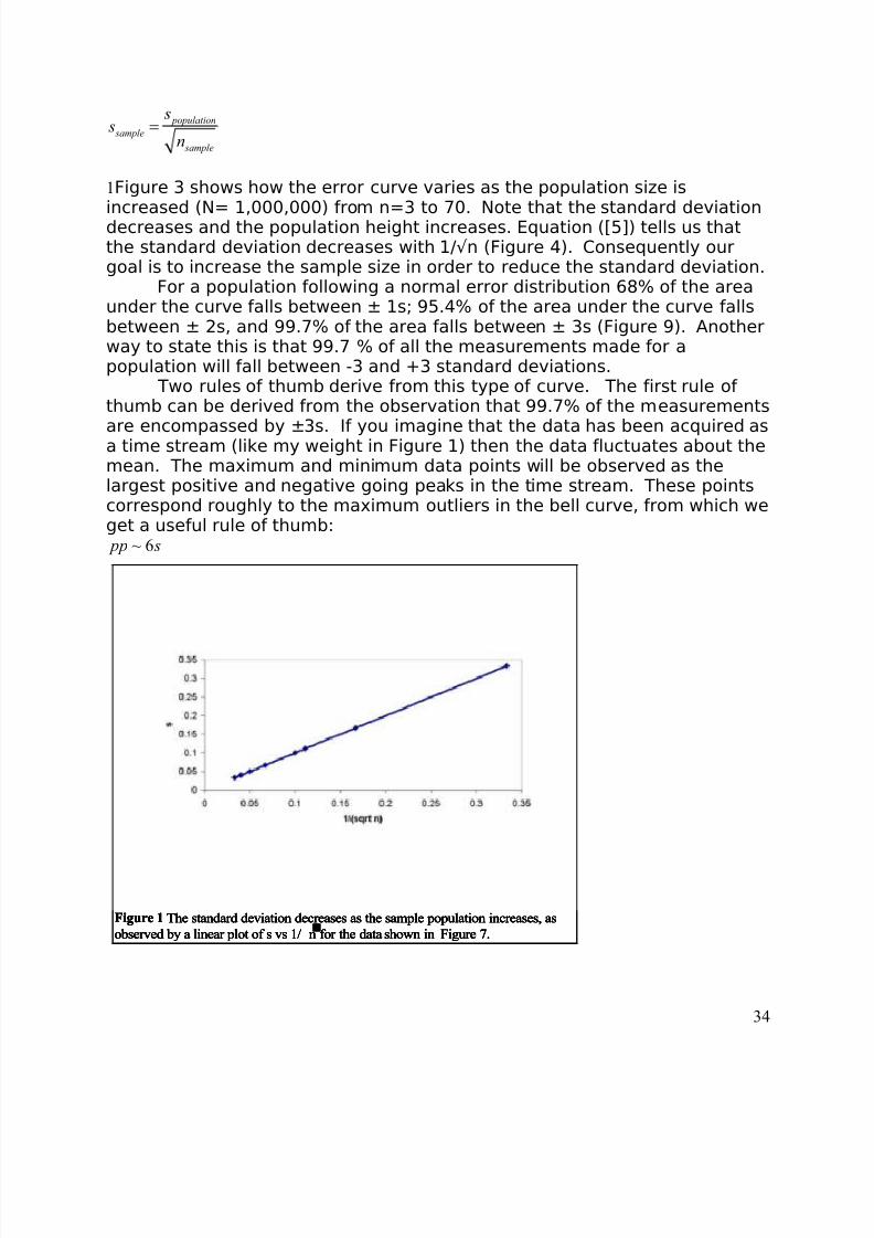
1Figure 3 shows how the error curve varies as the population size is

increased (N= 1,000,000) from n=3 to 70. Note that the standard deviationdecreases and the population height increases. Equation ([5]) tells us thatthe standard deviation decreases with 1/√n (Figure 4). Consequently ourgoal is to increase the sample size in order to reduce the standard deviation.

For a population following a normal error distribution 68% of the areaunder the curve falls between ± 1s; 95.4% of the area under the curve fallsbetween ± 2s, and 99.7% of the area falls between ± 3s (Figure 9). Anotherway to state this is that 99.7 % of all the measurements made for apopulation will fall between -3 and +3 standard deviations.

Two rules of thumb derive from this type of curve. The first rule of thumb can be derived from the observation that 99.7% of the measurements

are encompassed by ±3s. If you imagine that the data has been acquired asa time stream (like my weight in Figure 1) then the data fluctuates about themean. The maximum and minimum data points will be observed as thelargest positive and negative going peaks in the time stream. These pointscorrespond roughly to the maximum outliers in the bell curve, from which weget a useful rule of thumb:

~ 6 pp s

Figure 1 The standard deviation decreases as the sample population increases, as

observed by a linear plot of s vs 1/n for the data shown in Figure 7.







34

8/3/2019 2011 lab book V3


Figure 1 A normal error curve contains 68.3% of the measurements between ±1s ; 95.4% of the

measurements (area under curve) between ± 2s; and 99.74% of the measurements between ±3s.

Triangulation of the peak (drawing a line along each side of the curve through the inflection point,

estimates the peak base width between ±2s (4s total) and ±3s (6s total). The top of the peak

(between ±0.05s) accounts for 3.98% of the population of measurements.

Figure 1 A normal error curve contains 68.3% of the measurements between ±1s ; 95.4% of the

measurements (area under curve) between ± 2s; and 99.74% of the measurements between ±3s.

Triangulation of the peak (drawing a line along each side of the curve through the inflection point,

estimates the peak base width between ±2s (4s total) and ±3s (6s total). The top of the peak

(between ±0.05s) accounts for 3.98% of the population of measurements.

1where pp represents the peak to peak distance between the largest positiveand negative going peaks.

The second rule of thumb is that the area under a very narrowsegment at the peak contains a fixed proportion of the population (forexample ±0.05s contains 3.98% of all the individuals within the population)

(Figure 6). Therefore as the population size increases the peak height willscale also (e.g. 3.98% of n= 100 is 3.98 and of n=1000 is 39.8). For thisreason the peak height is often used to measure the intensity of a signal,assuming that the signal has a normal error shape.

To scale for the peak height the Gaussian equation is modified by apre-exponential factor, A, which is the peak height.

21

21( )

2

x

f x A e

µ

σ

σ π

− − =

1 The rule of thumb, peak height proportional to area under peak, fails whenthe population is skewed.

The third moment (Table 2) tells whether or not the population isskewed, or, in fact, an ideal, random population. The formula for the thirdmoment is given as:

35

8/3/2019 2011 lab book V3


( )3

21

n x x skew

ns

−= ∑

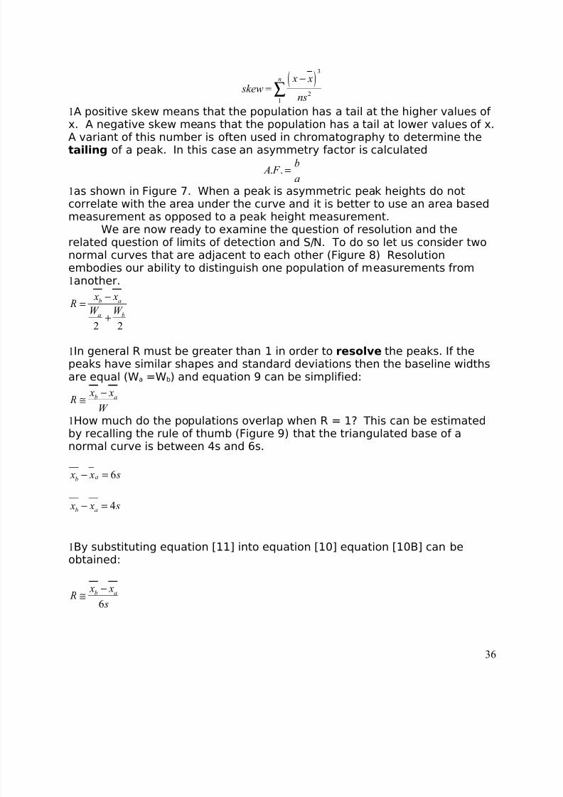
1A positive skew means that the population has a tail at the higher values of x. A negative skew means that the population has a tail at lower values of x.

A variant of this number is often used in chromatography to determine thetailing of a peak. In this case an asymmetry factor is calculated

. .b

A F a

=

1as shown in Figure 7. When a peak is asymmetric peak heights do notcorrelate with the area under the curve and it is better to use an area basedmeasurement as opposed to a peak height measurement.

We are now ready to examine the question of resolution and therelated question of limits of detection and S/N. To do so let us consider twonormal curves that are adjacent to each other (Figure 8) Resolutionembodies our ability to distinguish one population of measurements from

1another.

2 2

b a

a b

x x R

W W

−=

+

1In general R must be greater than 1 in order to resolve the peaks. If thepeaks have similar shapes and standard deviations then the baseline widthsare equal (Wa =Wb) and equation 9 can be simplified:

b a x x

RW

−≅

1How much do the populations overlap when R = 1? This can be estimatedby recalling the rule of thumb (Figure 9) that the triangulated base of anormal curve is between 4s and 6s.

6ab x x s− =

4b a x x s− =

1By substituting equation [11] into equation [10] equation [10B] can be

obtained:

6b a

x x R

s

−≅

36

8/3/2019 2011 lab book V3


4b a x x

R s

−≅

1In this class we generally use the first of equations [10B].If the means are 6s apart then each population “touches” when 3s has

been covered. The population that extends beyond 3s is (100-99.7)/2 =0.15%. Thus 0.15% of the population of A lies under the bell curve for thepopulation of B and vice versa. If the means are really only 4s apart thenpopulation A touches population B at 2s from the mean of A. The populationthat extends beyond 2s is (100-95.4)/2 = 2.3%. Thus a resolution of 1means that between 0.15 and 2.3% of the population could fall in the secondbell curve.

For our example involving vacation weights the resolution (usingequation 10B) of the vacation (not school!!) weight from the baseline weightis R = (141.9-140)/6(.329) = 0.96. Since R <1 we have not completelyresolved the vacation weight from the baseline weight. Resolution could be

accomplished by either having me gain more weight during vacation (changethe slope of the curve) or by having the standard deviation decreased (onlyweigh myself in the same clothes every day).

The limit of detection is similar to resolution as it is also based on theidea of overlapping bell curves. Analytical chemists consider that onepopulation can be detected when the mean signal for the population lies 3standard deviations away from the mean signal for the blank or baseline:

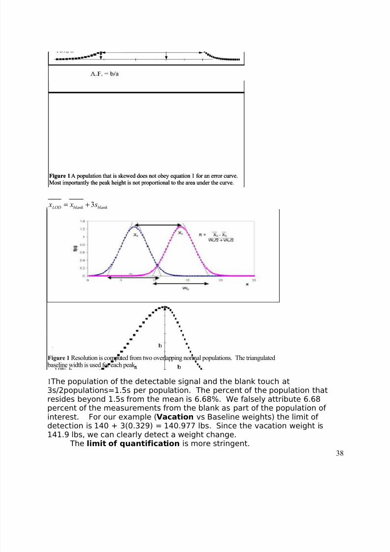
Figure 1 Resolution is computed from two overlapping normal populations. The triangulated baseline width is used for each peak.Figure 1 Resolution is computed from two overlapping normal populations. The triangulated

baseline width is used for each peak.

37

8/3/2019 2011 lab book V3


Figure 1 A population that is skewed does not obey equation 1 for an error curve.

Most importantly the peak height is not proportional to the area under the curve.Figure 1 A population that is skewed does not obey equation 1 for an error curve.

Most importantly the peak height is not proportional to the area under the curve.

3 LOD blank blank x x s= +

Figure 1 Resolution is computed from two overlapping normal populations. The triangulated baseline width is used for each peak.Figure 1 Resolution is computed from two overlapping normal populations. The triangulated baseline width is used for each peak.

1 The population of the detectable signal and the blank touch at3s/2populations=1.5s per population. The percent of the population thatresides beyond 1.5s from the mean is 6.68%. We falsely attribute 6.68percent of the measurements from the blank as part of the population of interest. For our example (Vacation vs Baseline weights) the limit of detection is 140 + 3(0.329) = 140.977 lbs. Since the vacation weight is141.9 lbs, we can clearly detect a weight change.

The limit of quantification is more stringent.38

8/3/2019 2011 lab book V3


9 LOQ blank blank x x s= +

1In our example (Vacation vs baseline weights) the limit of quantificationwill be 140 + 6(0.329) = 141.97. The weight change during vacation was

141.9 lbs so that we are not able to quantify the weight change.A very similar measurement is termed the signal to noise ratio S/N.

In this number the signal, S, is the difference between the mean of the signaland the mean of the blank, while the noise, N, is the standard deviation, s, of the blank:

signal blank

blank

x xS

N s

−=

1Referring to the time based plot of the weight gain (Figure 1) we note thatthere are fluctuations of weight around a mean in the area marked baselineand the area marked vacation. The distance from the maximum to the

minimum is termed the peak to peak fluctuation and was noted asapproximating 6s (equation 6). From this plot we can determine the S/N of the vacation weight as (140.977-140)/(142.8-141.2)/6) = 3.66.

Analysis of VarianceSuppose that the resolution between populations is small enough that

it is not immediately visually apparent, i.e. baseline resolution is notobserved and the peaks overlap to the extent that they appear as a singlelarge “lumpy” peak. How is this situation handled?

An example is to look at the histogram of weights in Figure 2 and applya statistical test to “resolve” the populations. The first step is to assume that

the bar graph in Figure 5 represents a random homogeneous population. Arandom population assumption allows us to make use of normal or Gaussianmathematics.

In order to assign confidence in our data we first assume that they canbe described by the normal curve formulas (equations 1-3). We thencompute the mean and standard deviation1(width) of our population, usethese numbers to compute the expected number of observations, and plotthis curve as an overlay of the histogram of real data. If the match is good(as measured by deviations from the histogram to the expectedobservations) then we accept the computation. If the match is poor then wemust check to see if we really have two or more populations. (An

examination of the Figure 1 shows that the error curves estimated from thesample population do not actually match the data very well).

As an example let's determine if the vacation weight is part of therandom fluctuations in weight with time or is truly a separation weightpopulation. We will perform an analysis of variance on the system asshown in Figure 9. The actual computation for an analysis of variance is rote(or by formula) but the concept behind the analysis of variance is to find a

39

8/3/2019 2011 lab book V3


theoretical population curve or curves that best matches the histogram(shown visually in Figure5). The tool by which a population is judged to fit a model of a single or amultiple population is the F statistic. This statistic computes the expectedmismatch between acquired data and the predicted population based on the

population size and the uncertainity one is prepared to expect. When thecalculated F value is greater than the expected F value there is too muchvariation in the attempt to match the data to a single population. Thealternative hypothesis, that the data is better described by two samplepopulations, is correct.

The best way to learn to do an ANOVA (analysis of variance) is to followthe example 1step by step. An ANOVA can also be calculated on a spreadsheet such as Excel.

Calibration Curve.Each measurement we make of the signal for a concentration consists

of a histogram of measurements centered around a mean signal with astandard deviation associated with the measurement. We can construct acalibration curve using these variable measurements. For the sake of argument, let us assume that the baseline weight (Figure 4) was associatedwith eating 1500 calories/day, the vacation weight gain was associated witheating 4000/day and the semester weight gain with eating 6000 calories/day. Using all the data shown we can construct a calibration curve (Figure10).

The “calibration” curve is constructed with two sets of data. The firstincludes all the weight measurements and illustrates the “scatter” of data,similar to the baseline of a Gaussian curve. The second set of data is

constructed from the mean of the scattered data and the standard deviationassociated with that mean for each calorie/day value. This data has beenused to create a regression curve which projects backward to the weightassociated with zero calories per day (how easy it is to “misrepresent” withstatistics!!!).

The errors associated with calibration curves are computed in a fashionsimilar to the ANOVA. The variability of all the measurements is the sum of the variability in the x population, the variability in the y population and thevariability along the line:

40

8/3/2019 2011 lab book V3


Sample Normal" Vacation Totals

i=1n j = 1 j = 2 j =1k 1 140 141.7

2 140.1 141.93 139.8 141.44 140.6 142.35 140 142.36 139.8 140.67 139.6 142.3

8 140 142.79 140.8 141.710 139.7 141.611 140.2

n j 11 10 n = 11+10=21

mean 140.05 141.85s 0.36705 0.5961s2 0.1347 0.3561

T j = inxij 1.5406x103 1.4185x103 T = T j = 2959.1

( xij)2 215769x105 2.01217.4 SS =416986.8

TSS = total sum squares = SS-(T2/n) = 21.4381

BSSS = between samples sum squares = j=1k (T j

2/n j) - (T2/n) = 16.885

BSMS = between sample mean square = BSSS/(k-1) = 16.885/(2-1) = 16.885

R = residual error = TSS-BSSS = 21.438-16.885 = 4.55

RMS = residual mean square = R/(n-k) = 4.55/(21-2) = 0.2395

Fcalculated > predicted at 5% probability of randomness then difference is significant

=BSMS/RMS = 16.885/0.2395 = 70.477Fk-1,n-1,α = F1,20,0.05 = 4.35 (from table)

Figure 1: An example calculation of analysis of variance (ANOVA) using the data from Figure 4. The

value for the theoretical F number is found in the appendix.

Sample Normal" Vacation Totals

i=1n j = 1 j = 2 j =1k 1 140 141.7

2 140.1 141.93 139.8 141.44 140.6 142.35 140 142.36 139.8 140.67 139.6 142.3

8 140 142.79 140.8 141.710 139.7 141.611 140.2

n j 11 10 n = 11+10=21

mean 140.05 141.85s 0.36705 0.5961s2 0.1347 0.3561

T j =inxij 1.5406x103 1.4185x103 T =T j = 2959.1

( xij)2 215769x105 2.01217.4 SS =416986.8

TSS = total sum squares = SS-(T2/n) = 21.4381

BSSS = between samples sum squares = j=1k (T j

2/n j) - (T2/n) = 16.885

BSMS = between sample mean square = BSSS/(k-1) = 16.885/(2-1) = 16.885

R = residual error = TSS-BSSS = 21.438-16.885 = 4.55

RMS = residual mean square = R/(n-k) = 4.55/(21-2) = 0.2395

Fcalculated > predicted at 5% probability of randomness then difference is significant

=BSMS/RMS = 16.885/0.2395 = 70.477Fk-1,n-1,α = F1,20,0.05 = 4.35 (from table)

Figure 1: An example calculation of analysis of variance (ANOVA) using the data from Figure 4. The

value for the theoretical F number is found in the appendix.

41

8/3/2019 2011 lab book V3


2 2 2

q x y xy

x

q q q q

x y y

∂ ∂ ∂ ∂ σ σ σ σ

∂ ∂ ∂ ∂

= + +

1where σxy is the variability along the line:

1

1 ( )( ) N

xy i line i line

i

x x y y N

σ =

= − −∑1 The differences between the measurement and the line should berandomly distributed in positive and negative directions, therefore the sumof the differences should go to zero. In this case the variance associatedwith an individual measurement should approach the randomness in the xand y populations:

22

2 2

2

2

1

x y

q

q q

x yr

∂ ∂ σ σ

∂ ∂

σ

+ =

−1What this equation states is that a good fit (r2 goes to 1) occurs when thevariance along the x axis summed to the variance along the y axis is close toor equal to the total variability of the 1data. We expect r to be >0.9 for agood linear fit to the data.

How good is good for a given population size? If we report an r valueof 1 for a two point line we have zero confidence in the value of r = 1,because we can always fit a straight line through two points. If r = 1 on aline with 100 points we are much more confident in the value of r. A line of three points with an r=0.9 would have a random chance of such acorrelation 29% of the time. Thus we are only 71% confident that the line isthe appropriate fit through the data. If we have a five point line with anr=0.9 we have a 3.7% change of random events giving us the line, or we are96.3% confident that the r value is accurate.

Another useful piece of information can be obtained by an analysis of the variability of the data in the regression. A backwards projection of themagnitude of error along the regression1line can be used to get an estimate of the variability associated with theintercept (blank). This is useful in cases where the analyst has fouled up andforgotten to obtain the requisite 3 measurements of the blank fordetermination of the standard deviation of the blank. An estimate of thestandard deviation of the blank can be obtained by error analysis of theintercept. Most standard statistical packages performing linear regressionswill give intercept error estimates. The error associated with the means andwith the fit to the line are used to also project backward the error barsassociated with the blank (see Figure 10).Wednesday, March 03, 2010

Creating a RegressionLineConfidence Plot using excel

42

8/3/2019 2011 lab book V3


(based on the web site: Author: Bernard Liengmehttp://people.stfx.ca/bliengme/ExcelTips/RegressionAnalysisConfidence2.htm )

Assume you have the following data:

Experimentaldata

x y0.0 8.98

12.0 8.14

29.5 6.67

43.0 6.08

53.0 5.90

62.5 5.83

75.5 4.68

85.0 4.20

93.0 3.72

A regression analysis by Excel gives you the following output:

SUMMARY OUTPUT

Regression Statistics

Multiple R 0.987152266

R Square 0.974469597

Adjusted R Square 0.970822396

Standard Error 0.296663064 SYX

Observations 9 n

ANOVA

df SS MS F

Regression 1 23.51449274 23.51449 267.1829

Residual 7 0.616062815 0.088009

Total 8 24.13055556

Coefficients Standard Error t Stat P-value

b Intercept 8.704027305 0.191564504 45.43654 6.54E-10

m X Variable 1 -0.053222152 0.003256028 -16.3457 7.82E-07

Highlighted in yellow are some of the values we will need to create our confidence limits plot: the standard error,Syx, the number of observations, n, the intercept, b, and the slope, m.We also need to calculate the mean (average) of the x values and the square of difference of each x value from thatmean, then sum:

Experimentaldata

x y 8301.39 SSX

43

8/3/2019 2011 lab book V3


0.0 8.98 2539.04

12.0 8.14 1473.71

29.5 6.67 436.35

43.0 6.08 54.60

53.0 5.90 6.82

62.5 5.83 146.68

75.5 4.68 630.57

85.0 4.20 1197.93

93.0 3.72 1815.71

average: 50.3889

The value in the third column is obtained as (x-50.3889)^2. The yellow highlighted value 8301.39 is the sum of thedeviation of x from the mean of x.

The last value we need is the t value for a given probability (or confidence we want) and degrees of freedomassociated with our regression (n-2). For this example n= 9 so n-2=7. To have a 95% confidence limits, we want 5%error so we type in to some cell”

=tinv(prob, deg free)=tinv(0.05,7)

The returned value is 2.365.

All of the necessary values are shown in Bernard Liengme’s examples as:

Derived values

Slope, m m -0.053 SLOPE(y,x)

Intercept, b b 8.704 INTERCEPT(y,x)

Observations, n n 9.000 COUNT(x)

Std error in estimate, Syx SYX 0.297 STEYX(y,x)Average x XAVG 50.389 AVERAGE(x)

SSX SSX 8301.389 DEVSQ(x)

t(α ,df) t 2.365 TINV(0.05,n-2)

To calculate the confidence limit (Cl):

=t*SYX*SQRT(1/n+(A18-XAVG)^2/SSX)

=(m*A18+b)+B18

44

8/3/2019 2011 lab book V3


Regression line confidence interval

x CI y+CI y-CI

0 0.45 9.16 8.25

10 0.39 8.56 7.78

20 0.33 7.97 7.3130 0.28 7.39 6.83

40 0.25 6.82 6.33

50 0.23 6.28 5.81

60 0.25 5.76 5.27

70 0.28 5.26 4.70

80 0.33 4.77 4.12

90 0.38 4.30 3.53

100 0.45 3.83 2.93

In this image A18 is the pink cell, Cl stands for confidence limit. Next calculate the range of y values that youwould expect from

( )[ ] Cl xbm y ±+=The third column predicts the value of y

( )[ ] Cl xbm y ++=While the fourth column predicts the lower expected value of y:

( )[ ] Cl xbm y −+=

Create a plot of the observed values of y as symbols and the predicted higher and lower limits of y as lines:

45

8/3/2019 2011 lab book V3


9.00

10.00

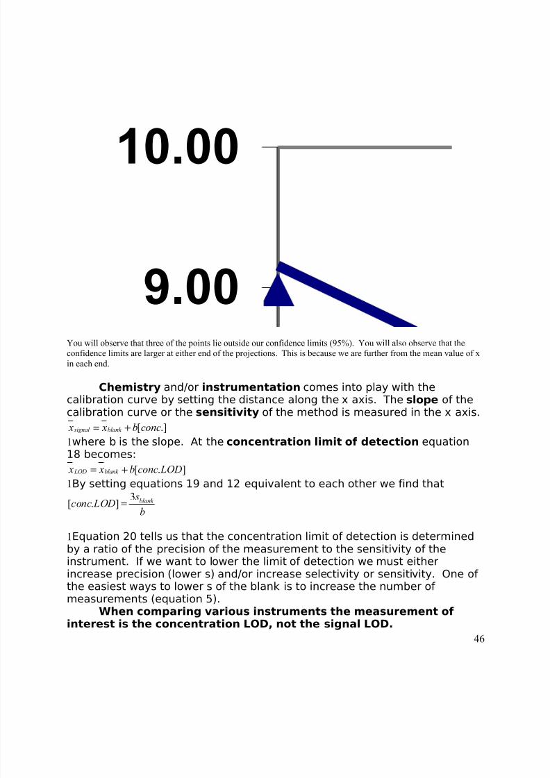
You will observe that three of the points lie outside our confidence limits (95%). You will also observe that theconfidence limits are larger at either end of the projections. This is because we are further from the mean value of xin each end.

Chemistry and/or instrumentation comes into play with thecalibration curve by setting the distance along the x axis. The slope of the

calibration curve or the sensitivity of the method is measured in the x axis.[ .] signal blank x x b conc= +

1where b is the slope. At the concentration limit of detection equation18 becomes:

[ . ] LOD blank x x b conc LOD= +1By setting equations 19 and 12 equivalent to each other we find that

3[ . ] blank

sconc LOD

b=

1Equation 20 tells us that the concentration limit of detection is determinedby a ratio of the precision of the measurement to the sensitivity of theinstrument. If we want to lower the limit of detection we must eitherincrease precision (lower s) and/or increase selectivity or sensitivity. One of the easiest ways to lower s of the blank is to increase the number of measurements (equation 5).

When comparing various instruments the measurement of interest is the concentration LOD, not the signal LOD.

46

8/3/2019 2011 lab book V3


Not only are LOD and sensitivity of the method important, but also thelinear range. The linear range is the concentration range over which asingle slope “b” applies. There are very few instrumental methods whichhave large linear ranges coupled to low limits of detection. Figure 11illustrates a typical instrumental calibration curve with the linear range

denoted.

47

8/3/2019 2011 lab book V3


Revised #2 2011 Matthew Reichert

Electronic Enhancement of S/N,

Frequency encoding, and BoxcarFiltering

Synopsis:Students are provided out put of data from an analog filter from which

they create a Bode plot and determine the time constant of the filter.Students are also provided with a set of data which they filter digitally bysliding boxcars and by waveform summation. Students create data for aFourier transform and apply a Fourier transform to the data.

Testable Skill Acquired1. Students continue to build familiarity with spreadsheet

manipulations2. Students reinforce ability to plot data on a spreadsheet3. Students reinforce the concepts of signal enhancement by

increased sampling4. Students perform a spreadsheet based Fourier Transform

smoothing of the data.5. Students perform boxcar filtering and wave form summations,

and demonstrate the concept of noise reduction proportional tosquare root of sample number

6. Students construct a Bode plot then determine the cut off frequency.

7. Students shift a signal’s frequency

Filtering DataAll of the “tricks” practiced below assume that any experimental data can beassumed to be the sum of a series of sin waves:

( )( )

( )( )

V V

nt n f

V V t n f

t

i

i

n

m e a s u r e d s i g n a l t i m e n o i s

=

= +

∑ s i n

s i n( )

2

2

1

π

π

(1 and 2)

In these first two filters the assumption is that the signal waveform isreproducible and the noise component is random.

48

8/3/2019 2011 lab book V3


The next three exercises illustrate methods of enhancing the signal rely uponthe fact that often noise is a high frequency component. Sometimes a signalis deliberately shifted in frequency to separate the signal from the noise.Much of the noise can be removed immediately before digitization of thesignal by application of a low pass filter. Alternatively signal can be

decomposed into its various frequency components and the noisefrequencies isolated and removed via a Fourier transform technique.

49

8/3/2019 2011 lab book V3


A. Sliding BoxcarIn the boxcar digital filtering the assumption is that any noise added to

the signal has equivalent excursions positive and negative from theunpolluted signal. As a consequence an average of a series of closelyspaced points should result in destructive interference of positive and

negative excursions:

1. Open the spreadsheet for the Boxcar exercise..2. To form a 3 point sliding boxcar, in cell E11 type

=average(D10.D12)Copy this formula to the cell E205. You should 1 less data point at thetop and bottom of your 3 boxcar data than in the original raw data.

3. To from a 5 point sliding boxcar, in cell F12 type=average(D10.D14)

Copy this formula to cell F204. You should have 2 less data points atthe top and bottom of your 5 boxcar data than in the original raw data.

4. To from a 7 point sliding box car, in cell G13 type=average(D10.D16)

Copy this formula to cell G203. You should have 3 less data points atthe top and bottom of your 7 boxcar data than in the original raw data.

6. To form a 9 point sliding boxcar, in cell H14 type=average(D10.D18)Copy this formula to cell H202. You should have 4 less data points

at the top and bottom of your 9 boxcar data than in the original rawdata.

7. To form a 25 point sliding boxcar in cell I22 type=average(D10.D34)Copy this formula to cell I96. You should have 12 less data points atthe top and bottom of your 9 boxcar data than in the original rawdata.

8. Produce a graph showing what happens to your data as the size of the boxcar increase

50

8/3/2019 2011 lab book V3


B. Waveform SummationFor waveform summation the noise should decrease because the

standard deviation of a population decreases with the number of measurements:

( ) s x x

n

n2

2

1 1= −

−∑ (3)

If we consider a theoretical population consisting of a large number of individuals, N, with a population standard deviation of spop of which we onlysample a few members, n, then the standard deviation of the sample, ssam,scales with the number of individuals sampled:

sn

N

s

n s a m p l e

p o p u2

2

1= −

(4)

If N is very large (10,000) compared to the sample size (1-100) thenequation 4 reduces to

s s

n s a m p l e

p o p u l

s a m

= (5)

This last equation indicates that as the sample size increases the standarddeviation of the sample will decrease.

1. In your excel sheet go to tab “16 waveforms”.2. Average waveforms 1 through 4; 1 through 9 and 1 through 16.

3. Determine noise of waveform 1, average of 1 through 4,average of 1 through 9 and average of 1 through 16waveforms. The noise is pp/6. The waveform you have is asine wave. Expand your graphs to the point that the top of the sin wave is nearly flat to make the peak to peakmeasurement.

4. Plot the noise as both a function of the number of waveforms (1, 4,9, and 16) and as a function of the sqrt of the number of averagedwaveforms. Which is a better plot? Why?5. What will happen if you shift the data of one waveform slightlydown so that it is out of phase?

51

8/3/2019 2011 lab book V3


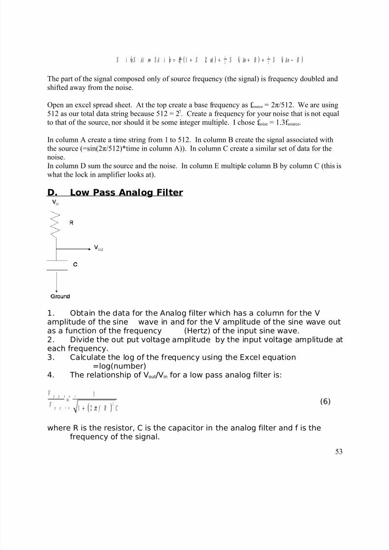
C. Frequency Encoding the Sample. Frequency encoding is accomplished by putting the source beam on a chopper so that thesignal generated is tied to a known frequency, while the background (noise) is on some baselineor variable frequency. What this allows you to do is to recover the signal frequency and removethe noise frequency through the use of a lock-in-amplifier . The way it works is the following.

The source is chopped onto a frequency, f source, with an amplitude Asource

( ) ( ) I n t e n i s y A f t s o u r c e s o u r c e s o u r = s i n2 π

The source beam is sent to the sample cell where it is altered by interaction with the sampleleading to a different amplitude:

( ) I n t e n i s y A

xf t s i g n a l

s o u r c e

s o u r =

s i n2 π

While in the sample cell noise is collected that has its own peculiar frequency, f noise

( ) I n t e n i s y A f t n o i s e n o i s e n o i s= s i n2 π

The detector observes the sum of the sample intensity at the source frequency and the noise

intensity at the noise frequency

( ) ( ) I n t e n i s y A

xf t A f t e c t o r

s o u r c e

s o u r c e n o i s e n o i sd e t s i n s i n=

+2 2π π

To get only the sample intensity a clever trip is pulled. The output of the detector is multiplied by the source frequency:

52

sourcechopper Source signal

noise

Reference beam

Signal beam

multiplysourcechopper Source signal

noise

Reference beam

Signal beam

multiply

8/3/2019 2011 lab book V3


( ) ( ) ( ) ( )S i n AS i n AS i n B S i n A S i n A B S i n A B+ = + + + + −12

12

121 2

The part of the signal composed only of source frequency (the signal) is frequency doubled andshifted away from the noise.

Open an excel spread sheet. At the top create a base frequency as f source = 2π/512. We are using512 as our total data string because 512 = 27. Create a frequency for your noise that is not equalto that of the source, nor should it be some integer multiple. I chose f noise = 1.3f source.

In column A create a time string from 1 to 512. In column B create the signal associated withthe source (=sin(2π/512)*time in column A)). In column C create a similar set of data for thenoise.In column D sum the source and the noise. In column E multiple column B by column C (this iswhat the lock in amplifier looks at).

D. Low Pass Analog Filter

1. Obtain the data for the Analog filter which has a column for the Vamplitude of the sine wave in and for the V amplitude of the sine wave outas a function of the frequency (Hertz) of the input sine wave.2. Divide the out put voltage amplitude by the input voltage amplitude ateach frequency.3. Calculate the log of the frequency using the Excel equation

=log(number)4. The relationship of Vout/Vin for a low pass analog filter is:

( )

V

V f R C

p p o u t

p p i n

=+

1

1 22

π (6)

where R is the resistor, C is the capacitor in the analog filter and f is thefrequency of the signal.

53

8/3/2019 2011 lab book V3


When:

R C f

=1

2 π

(7)

the ratio of the out put signal to input signal is:

V

V

o u t

i n

=+

= =1

1 1

1

20 7 0

2. (8)

A plot of V

V

o u

i n

vs. log Hz is called a Bode plot. Locate on your Bode plot the cutoff frequency where Vout/Vin is

0.707. From the frequency determine the RC value from equation (8). What is the bandwidth (frequency range that

is passed) of this low pass filter?

E. Fourier Transform Exercise

In the equation below there are 9 different sin waves each a multiple of abase frequency (1) with an amplitude scaled to the base frequency asshown in the frequency plot below.

( )( ) ( )( ) ( )( ) ( )( )V V f t V

f t V

f t V

f t V

f t t = + + + +1

1 1 1 12

32 3

52 5

72 7

1 72 1 7s i n ( ) s i n s i n s i n . . . . s i nπ π π π π (9)

12000

54

8/3/2019 2011 lab book V3


The equation, which represents, the sum of nine individual sin wavesapproximates a square wave when plotted in the time domain:

15000

e

As seen above every time varying signal can be considered a sum of sin waves. Another way to express the summation of sin waves is as a Fourier series:

( ) ( ) ( ){ } f x A a x B a xd = +∞

∫ α α c o s s i n0

(10)

where the amplitudes of A(α) and B(α) are themselves integrals of sin waves.A Fourier transform of the time varying data in equation (6) to reveal thefrequency dependent data is obtained by the function:

( ){ } ( ) ( )ℑ = =− ∞

∞−∫ f x F x f x e d i a x

(11)

This math manipulation can be discretized to work in a spreadsheet as

( ) ( ) F x f x W m N n m

x

N

= ==∑ , , , . . . .1 2

1 (12)

55

8/3/2019 2011 lab book V3


Solution of N

2

multiplication operations are required which made it an

undesirable application. However performing the operation as a matrix set

results in a fast Fourier transform (FFT) which can be used even within fairly

simple computational packages including Excel.

This is very useful because an analog signal converted to a digital set

of data within the computer can be manipulated by the FFT transform to

derive a frequency spectrum of the signal. If the source of the noise is

known it can be removed from the frequency spectrum and the time domain

signal reformed minus noise.

The point of this exercise is to transform the unfiltered data. Since you have artificiallyconstructed the unfiltered data (a square wave) from different frequency sin waves a transforminto F.T. space should yield back information about the different frequencies. The F.T. can be performed in Excel, but takes a little bit of trickery.

Fourier Transform by Excel

To perform a fast Fourier transform by excel your time varying data must be a string (in acolumn) that is 2n long (2, 4, 8, 16, 32,512....). The digital FT performed by excel does not makereference to your measured time, but treats your data as a string of data from n to 2n.

Open an excel spread sheet. At the top create a base frequency as f source = 2π/512. We are using512 as our total data string because 512 = 27.

In column A create a time string from 1 to 512. In column B create the signal associated withthe source (=sin{(2π/512)*(time in column A}). The sin function should include (2πtime/512).

In subsequent columns create the higher frequencies required to obtain a square wave:

( )( ) ( )( ) ( )( ) ( )( )V V f t V

f t V

f t V

f t V

f t t = + + + +1

1 1 1 12

32 3

52 5

72 7

1 72 1 7s i n ( ) s i n s i n s i n . . . . s i nπ π π π π

where V1 is the amplitude (V1 = 1 for this analysis) and 2πf is the source frequency. In the finalcolumn create a square wave by summing all of the sin waves. Plot this to see that you doindeed have a square wave.

56

8/3/2019 2011 lab book V3


Calculate the rise time of the signal. The rise time is the measure of time it takes the instrumentto move from 10% to 90% of the full signal. It is a measure of how fast you can make themeasurement with out distortion. The rise time is expressed as:

( ) f f f

t r

∆=

−=

3

1

2

1

12

It can be seen that the rise is inversely related to the range of frequencies in the measurement.The higher the range of frequencies (bandwidth) the faster the rise time (that’s a good thing!).For modern op amp based instruments there is no low frequency roll of so that t r is defined only by the high frequency roll off point

( ) 212 3

1

3

1

2

1

f f f f t r ≈

∆=

−=

Rise time

10%

90%

Sin(f)

Sin(f) +1/3sin(3f)

Sin(f) +1/3sin(3f) +1/5sin(5f)

Sin(f) +1/3sin(3f) +1/5sin(5f)+1/7(sin(7f)

Open the tools pack and go to Fourier transform. Specify the 512 data points associated with thedetector (the summed data). Tell it to place the transformation in the column next to the summeddata.

The transformed data placed will be a complex number representation of the amplitude of thefrequency components for 0 (f source), then 1(f source), then 2(f source) and so on. (An aside: we havedeliberately created our source frequency to pass one cycle in 512 second. If you use the FFT in

other applications, the fft considers the fundamental period of the frequency to be what happens

in the 512 data points you scan). The first point in the column of transformed data willrepresent 0 frequency, or DC. Each sequential box will represent the amplitude of frequency 1

57

8/3/2019 2011 lab book V3


(1cycle/512 second), frequency 2 and so forth up to point 256 at which point the numbers displaythe amplitude of each decreasing frequency.

The data displayed is a complex number. To convert to something you can graph create another containing the equation =imabs(transformed data column).

Create a histogram of the imabs column. You do not need to use the Histogram package in

Excel or to create bins here. Simply highlight the data in column F including only the 2nd

through the ~ 30 data points (base frequency to frequency multiple 30). Using that singlecolumn insert a bar graph. The computer will automatically assign numbers 1, 2..... to your xaxis. The data you highlighted will be the y axis or height of the bar graph. In this bar graph youshould see at least two frequency components. One component is the base frequency or signal

and the second is the high frequency noise sitting on top of it.

To filter the data create another column. Every number in this column should be zero except for the point representing the base frequency (point 2 in the column containing the transformed

data). Copy the complex number in column of transformed data over. Note, for someunexplained reason you will find a duplicate of this number at the end of the data string. Copythe complex number at the end of the column that is identical to the one you just copied as well.

Now re-create a time string of data by performing the inverse fft on the column of the copied andfiltered fft data. To do this, go to tools, Fourier Transform. In the Fourier Transform command box you click inverse. Tell the computer to place the data in an unused column. This data needsto be truncated. To truncate the data type =value(column) into the neighboring column.

Now plot the data from the previously created column as an xy scatter plot. You should see a beautiful noise free sin wave identical to the original noise free sin wave you generated or acquired.

Report:

In addition to introduction, materials, methods, and data, results, and dataanalysis use all of the following questions to construct an essay. Do notwrite the answers out question by question. Integrate them into acoherent essay. You may wish to consider other issues not listedbelow.

1 How does this type of analog filtering of sine waves relate to conceptsdiscussed in the statistics lab?

2. How can the circuit be reconfigured to create a high pass filter?3. What would be the cut-off frequency of this high pass filter?

4. When you observed the Signal summed to the Noise did youobserve a "beat" frequency?

58

8/3/2019 2011 lab book V3


5. Why does the boxcar averaging lower the amplitude of the highfrequency component?6. In what way does the amplitude of the high frequency component vary

with the size of the boxcar. Be very specific both in words and in mathand graphs. (Hint compute s from the peak to peak variation of the

high frequency component).7. Do you think that it is appropriate to average five points together evenwhen the signal is clearly variable with time? Would it be appropriateto average 100 points together? Why or why not? What might be abetter way of averaging the data?8. How does the S/N change when you sum waveforms? What

might be a problem in summing a waveform?9. Which worked best: FT or summing or boxcar?10. What would be a problem with doing a mathematical FT?11. How well did your frequency encoding work? Using the

examples in this dry lab how might you clean up the noise from

the encoded signal?12. What is meant by the rise time? Did any of your data relate to theconcept of rise time?

59

8/3/2019 2011 lab book V3


Extraction

MethodsHot Plate Acid Digestion (EPA 200.2)Sequential Soil ExtractionsMicrowave Digestion

60

8/3/2019 2011 lab book V3


Hot Plate Digestions

SYNOPSIS: Samples to be used the rest of the semester will beprepared and stored. The

general procedure is that given as a standard by the EPA. The digestedsample will be measured on all instrumental methods in the rest of thesemester.

PROCEDURE:

1. Obtain 11 50 mL beakers.3. Mix the sample thoroughly to achieve homogeneity. Pick out debris

and bugs. Grind soil to small particle size. Weigh five 1.00 g samplesinto separate erlenmeyer flasks. Weight a sixth sample into a weighingdish, label and set aside to air dry. Reweigh during the next lab

section. This will be your control for the dry weight of the soil.4. Place a weighing dish on the balance. Note the dish weight and/or tareto zero. Successively inject aliquots of de-ionized water each timenoting the new successive weight. Determine the relative standarddeviation associated with the pipette volume.

5. To two of the soil samples and one empty (three total) flasks, add 100uL of 1000 ppm Pb standard. The two soil spikes and the one soil-lesssample will constitute controls, as will the one soil-less lead-lesssample.

These steps will take about 1-1.5 hours.6. In hood, to each flask, add 10 mL of 1:1 HNO3:H2O, mix and cover with

a watch glass and heat to 95C, without boiling, for 15 minutes. A Diallevel of about 3 on the hot plate should be approximately right. Cool.(You may speed up cooling by placing the erlenmeyer flask in a largerbeaker filled with cold tap water). Add 5 mL of concentrated HNO3,heat without boiling for 30 minutes to complete the oxidation.Elevate the watch glass on a bent piece of glass tubing and evaporateto 5 mL without boiling.The entire step 6 will take about 1-1.5 hours.

7. Cool, add 2 mL water and 3 mL of 30% H2O2. Warm on hot platecovered. "Care must be taken to ensure that losses do not occur dueto excessively vigorous effervescence." Heat until end of bubbling.

Elevate the watch glass on a bent piece of glass tubing and evaporateto 5 mL without boiling. Step 7 will take about 2 hours.

8. Cool and dilute in a volumetric with de-ionized water to 100 mL.9. Let sediment by sitting overnight and remove supernatant to acid-

washed basic EDTA rinsed storage bottle. Label.

61

8/3/2019 2011 lab book V3


REPORT In addition to materials, methods, and results your report shouldinclude the following information:

1. How will you make use of the controls?2. Why is HNO3 used and not HCl (or H2SO4) to digest your sample? At

what temperature does NO3

-

decompose? (See Chapter 7: equation7.5, incinerators).3. Why can't you boil your samples?4. How long do you need to digest the sample to get all the lead out?5. In what chemical forms will lead most likely be in your soil sample?

Which will be hardest to solubilize?6. Would you expect soils near a galena ore body (vol. i) to have the

same rate of digestion as soils in an urban playground?7. What implications might this have for the bioavailability of lead when

ingested?8. What materials in this lab would you consider hazardous?

9. Give a chemical reason for acid rinsing and EDTA rinsing your storagebottles.

62

8/3/2019 2011 lab book V3


Sequential Soil Extractions

SYNOPSIS In order to determine the availability of the soil lead, the soilmay be extracted with sequentially more powerful extractants. The method

shown below is based on that of Soon and Abboud:

PROCEDURE

1. Extract soils with distilled deionized (DD) water:a. Weigh 3 g of air-dried (<2 mm) soil into 120 mL

Erlenmeyer flask and add DD water.b. Shake soils for 2 hours 120 cycles/min with pure

water.c. Filter through a Whatman No. 42 filter paper.d. Save supernatant.

2. Extract soils with 1 M ammonium acetate/acetic acid (pH 7).3. Extract soils with dilute 1 M HNO3:a. 1 M HNO3: add 250 mL of concentrated HNO3 to 3 L

of distilled deionized water and dilute to 4 liters.b. Weigh 3 g of air-dried soil (< 2 mm) into a 125 mL

Erlenmeyer flask and add 30 mL of 1 M HNO3

extractant.c. Shake at 2 hours at a speed of 120 cycles/min.d. Filter through a Whatman No. 42 filter paper. Save filtrate for

analysis.4. Extract soils with EDTA:

a. 0.05 M EDTA (pH 7): dissolve 93.05 g of EDTA (di-sodium salt) in approximately 4 L of distilled anddeionized water (DD). Adjust to pH 7.0 with 7 MNH4OH, and make up to 5 L with DD water.

b. Weigh 5 g of air-dried (< 2 mm) soil into a 125 mLErlenmeyer flask and add 25 mL of 0.05 M EDTAsolution.

c. Shake for 1 hour at a speed of 120 cycles/min.d. Filter through a Whatman No. 42 filter paper after

shaking, save filtrate for analysis.

5. Extract with concentrated HNO3 and peroxide:a. Follow instructions given for a single total extraction of lead

(Experiment 10 )

Report In addition to title, introduction, materials and methods, include anessay based on the following questions:

63

8/3/2019 2011 lab book V3


1. Compare your extraction procedure to the possible forms of leadin the soil. Suggest what soil chemical form will be released (hintconsider solubilities) with each form of the extractant.

2. Which one will be most likely to relate to the acid digestible form of lead in a stomach acid environment?

3. From a public health standard, how will you interpret your resultsfor a single total lead acid digestion?4. Would you suggest that the cost of sequential extractions would beworthwhile for public health surveys?

64

8/3/2019 2011 lab book V3


Microwave Digestions

65

8/3/2019 2011 lab book V3


Commercial Spot Tests Synopsis: Students make spot tests of lead content using a commercial

stick.

READINGS Pages 269-273 in Critical Reviews

Procedure 1. Obtain three commercial lead sticks from the hardware store.2. To one: apply a drop of 1000 ppm Pb to the end of the stick and let

dry. Observe any color developed.3. To the second, apply a drop of 100 ppm Pb to the end of the stick and

let dry. Observe any color developed.4. To the second: apply a drop of 1000 ppm Zn to the end of the stick

and let dry. Observe any color developed.

Report

1. Was there a color difference between 100 and 1000 ppm Pb?2. Did Zn give a positive test on the lead stick? Wh or why not? What

implications might this have for using the gravimetric method of analysis with a soil sample digest?

1Articles on spot tests:

Ranyuk, Elena et al. Organic Letters 2009, Vol II, 4, 987-990 Diaminoanthraquinone-Linked Polyazomacrocycle: Efficient and Simple colorimetric Sensor for Lead in Aqueous Solution..

66

8/3/2019 2011 lab book V3


Revised 1/2011 Maria Kamm111 Chelation by Dithizone

Extraction + UV-VisSYNOPSIS Lead is selectively removed from an aqueous phase into an

organic phase by a chelating agent. The molecular electronictransition of the chelating reagent is perturbed by the presenceof lead causing a UV-Vis absorption band which can bemonitored. The selectivity of the process will be monitored bydifference spectroscopy in the presence of Zn2+. Students alsolearn how to deconvolute a spectra to account for backgroundabsorbance.

READINGSRead pages 304-309 in the Critical Reviews. Review the sectionon soluble lead chemistry on pages 273-279. Attached is anarticle describing some of the chemistry of dithizone. Theattached article is not as complete as the Critical Reviewsdiscussion.

Testable Skills 1. Ability to perform a deconvolution on a set of experimental data

2. Create a baseline subtracted standard curve3. Explain why UV-Vis absorption bands can be

considered to be Gaussian in shape in the

frequency domain.4. Explain the chemistry of the dithizone method.

The Dithizone Method This method was the first truly sensitive measure of lead. Adoption of

its use lead to the discovery of wide spread child lead poisoning in Baltimorein the 1930s. The method relies upon the development of a UV-Visabsorption band for a complex of lead dithizone that is resolved from theabsorption bands of the unreacted dithizone.

67

8/3/2019 2011 lab book V3


Because the lead band is resolved from the complex it can be measured inthe presence of the unreacted dithizone.

Despite the fact that the lead dithizone peak is reasonably resolvedfrom the unreacted dithizone the absorbance measured is the sum of bothreacted and unreacted dithizone:

A A Am e a s u r e d u n r e a c t e dl e a d d i t h i, , ,5 5 5 5 5 5 5 5 5= + − [1]

To get an accurate calibration curve you must subtract the absorbancecontribution of the unreacted dithizone. There are three ways to do this.

Method 1. The first is to create two calibration curves for the puredithizone. One calibration curve should be at a wavelength that isunaffected by the presence of the lead dithizone (for example ~640-680nm). Determine the molar absorptivity for free dithizone at this wavelengthfrom the slope of the calibration curve and the known thickness of thecuvette (typically 1 cm).

( ) [ ] A b F r e ed i t h i f r e ed i t h i z o z n e6 8 0 6 8 0= ε , [2]

The second calibration curve should be at the wavelength at which you willmeasure the complex (555 nm). Again, determine the molar absorptivity of the free dithizone at this wavelength from the slope of the calibration curve.

( ) [ ] A b F r e ed i t h i f r e ed i t h i z o n e f r e ed i t h i z o z n e5 5 5 5 5 5, ,= ε [3]

Solve the two equations for the absorbance contribution from free dithizone

at 555nm.

68

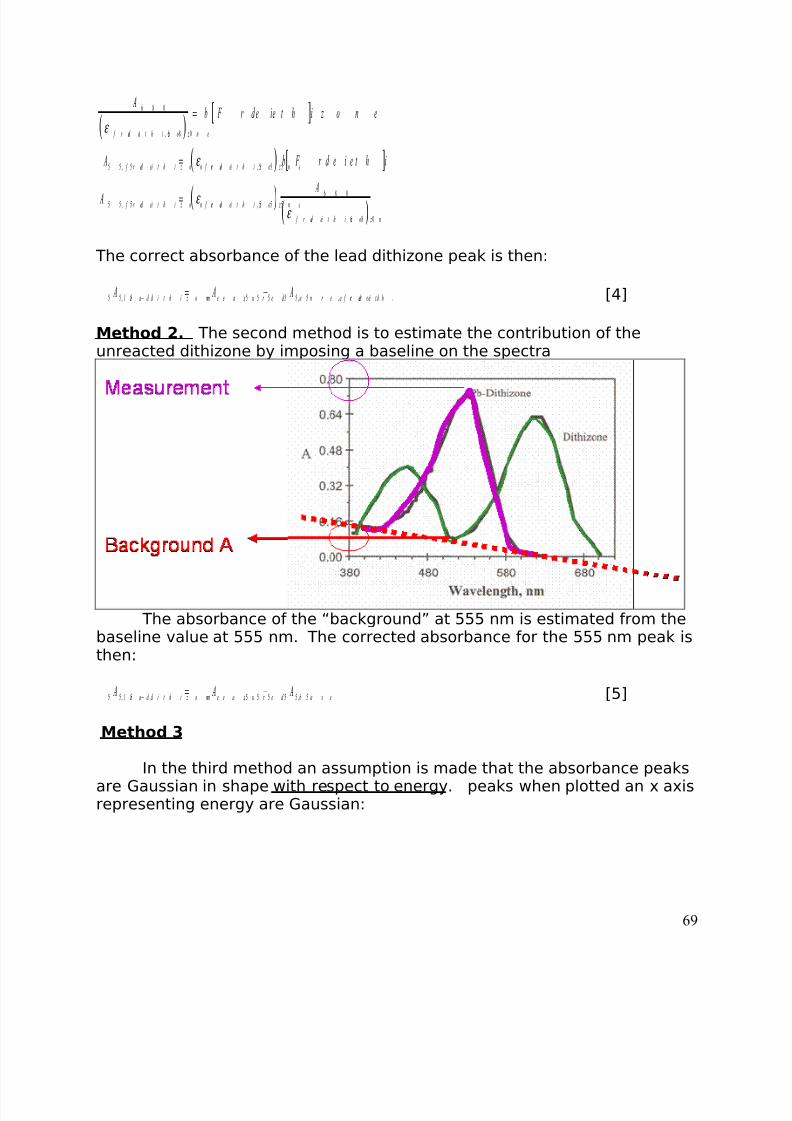
8/3/2019 2011 lab book V3


( )[ ]

( ) [ ]

( ) ( )

Ab F r e ed i t h i z o n e

A b F r e ed i t h i

A A

f r e ed i t h i z o z n e

f r e ed i t h i z o n e f r e ed i t h i z o z n e

f r e ed i t h i z o n e f r e ed i t h i z o z n e

f r e ed i t h i z o z n

6 8 0

6 8 0

5 5 5 5 5 5

5 5 5 5 5 56 8 0

6 8 0

ε

ε

ε

ε

,

, ,

, ,

,

=

=

=

The correct absorbance of the lead dithizone peak is then:

A A Al e a d d i t h i z o n em e a s u r e d u n r e a c t e d f r e ed i t h i5 5 5 5 5 5 5 5 5, , , ,− = − [4]

Method 2. The second method is to estimate the contribution of theunreacted dithizone by imposing a baseline on the spectra

The absorbance of the “background” at 555 nm is estimated from thebaseline value at 555 nm. The corrected absorbance for the 555 nm peak isthen:

A A Al e a d d i t h i z o n em e a s u r e d b a s e5 5 5 5 5 5 5 5 5, , ,− = − [5]

Method 3

In the third method an assumption is made that the absorbance peaks

are Gaussian in shape with respect to energy. peaks when plotted an x axisrepresenting energy are Gaussian:

69

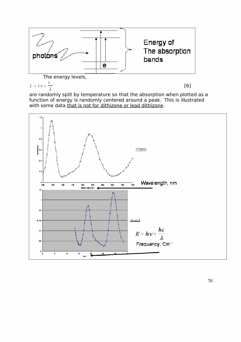
8/3/2019 2011 lab book V3


The energy levels,

E hh

= =ν λ

[6]

are randomly split by temperature so that the absorption when plotted as afunction of energy is randomly centered around a peak. This is illustratedwith some data that is not for dithizone or lead dithizone.

70

8/3/2019 2011 lab book V3


Notice that the peaks swap position on the x axis, but more importantlybecome distinctly more “Gaussian” in shape, and, as such, can be modeledas Gaussians.

In a previous lab we introduced the normalized Gaussian:

y

x

=

−−

1

2

1

2

σ π

µ

σ

e x p [7]In order to match the peak heights in this lab we use:

y A

x

=−

−

e x p

1

2

µ

σ [8]

In the next graph the data has been modeled as individual Guassians (dottedlines) summed. The summed Gaussian is subtracted from the measuredabsorbance, the difference squared, and plotted (dashed line). Notice thatfor this particular plot the sum of squared difference is large, indicating thatthe estimated Gaussian fit is poor.

1.2

In the next plot the sum of squared differences has gone very nearly to zero,indicating that a good fit has been obtained:

71

8/3/2019 2011 lab book V3


1.2

r b a n c e

Once a “good” fit is obtained the contribution of each band to the signal can be taken from theindividual peak heights. In the figure above for example, the absorbance at 22 cm-1 is the sumtwo contributions each of which can be determined.

72

8/3/2019 2011 lab book V3


INSTRUMENT 845 UV-Vis systemIn the soft ware you will be integrating data over a period

of time. Watch the count time! (How does that relate to1

N σ ∝ and the

quality of your data?)

GLASSWARE Six 100 mL volumetricsSeparatory flaskAssorted BeakersMicropipettes, 2 mL pipette, 5 mL pipettes

SOLUTIONS The dithizone must be made fresh on the day of use as it is unstable.

(How would you prove this to yourself?)

Wash bottle of acetone

10 mg dithizone/L Methylene chloride, CH2Cl2 The solvent should be pure from the manufacturer. If not

can lead to major problems with the method.20 g of KCN diluted to 1 L in the buffer (can omit, but what is the

purpose?)Buffer: 225 mL of 0.2 M sodium carbonate, 25 mL of 0.2 M sodium

bicarbonate, diluted to 1000 mL. (0.2 M anhydrous sodiumcarbonate from 21.2 g in 1000 mL; 0.2 M anhydroussodium bicarbonate from 16.8g in 1000 mL) results in pH11.

1000 ppm Pb stock solution.

1000 ppm Zn stock solution

CAUTION!!!!!If you use gloves to protect your hands from the organic reagents the

gloves should be free of powder as the powder will cause a false positive. This lab was a staple (standard method) for 40 years, but any lack of cleanliness will cause this method to fail.

PROCEDURE

A. Wavelength scanning.1. Set the range (F2) to 400-700 nm. Run blank (methylene

chloride) (F8).2. Scan 2 mL of 0.001% dithizone in CH2Cl2 solution over 400nm to

700 nm.Set the y scale to some preset value and print. Also, export datafor further work in Excel.

73

8/3/2019 2011 lab book V3


Repeat this experiment with new additions of dithizone in CH2Cl2three times.

WHY??

3. Add 5 ml of stock dithizone/CH2Cl2 solution to a separatory flask.

Add 100 μL of concentrated NH4OH (What is the purpose of NH4OH?) and 100 μl of 1000 ppm stock Pb. Shake 15-20seconds. Measure the exact number of seconds. Do notestimate. One student should be shaker and should use thesame shaking procedure every time. The green dithizonesolution should turn "carmine" red or pink. Wait for the phasesto separate. Remove the organic layer of the solution frombottom of separatory funnel and monitor it's absorbance from400nm to 700 nm.

4. Superimpose the plots of the dithizone and the lead and note

the region where the lead chelate absorbs as compared to thefree dithizone.

5. Export and save data to an excel format.

B. Calibration curve. For this method you should be able to get a calibration curve linearfrom 0.1 to 4 ppm. You will have to make these solutions up.

1. Place 10 mL of lead standard in separatory funnel. Add 4 mL of dithizone solution and 10 ml of buffer solution. Shake well for 1

minute. Measure this time exactly with a second handwatch. Allow the phases to separate. Pull CH2Cl2 solution frombottom of separatory funnel scan between 400 and 700 nm.Export the data.

2. Rinse the cuvette and funnel with MeOH and then acetone betweensamples.

3. Repeat for the Zn standards.

C. Background Correction for the Calibration Curve by Deconvolution

Use Excel to deconvolute the spectral data. Deconvolution is

necessary in this experiment because there will be a large amount of unreacted dithizone present which will cause the baselines to varysubstantially. If you measure the peak absorbance and plot it vs theadded lead you will often get poor calibration curves because the peakabsorbance contains absorbance from the un-reacted dithizone.

74

8/3/2019 2011 lab book V3


1. Open your data in excel.. You should have the wavelength incolumn A, and the absorbance in column B. Insert a new columnbetween A and B. In cell b2 type the formula: =10,000/A2 andcopy down to the end of data in column A. This represents thereciprocal of the wavelength (1/nm) which is a measure of

energy.2. Insert 10 rows, so that the labels for the columns are in row 11.3. In column D, rows 4 through 7 type the following labels: peak

frequency, peak A, s.4. In cells E11 through J11 type the labels: band1, band2, band3,

band4, sum, sqr diff. In cell J8 type the label “sum sqr diff”.5. Find your peak frequencies, and peak absorbances by plotting

1/nm vs A. You should find a major peak frequency of interestnear 0.002 1/nm and some other peak at different locations.

6. Estimate the standard deviation of the peaks from the basewidth of the peaks.

7. In cells E4, E5, and E6 enter your band1 peak frequency,absorbance and standard deviation. Do this for each of thebands you think you have. (You may need to insert columns, if you think you have more than 4 bands).

8. Compute the signal contributed by band 1. Type in cell E13=E$5*(EXP(-0.5*(($B13-E$4)/E$6)^2))Copy down to the end of the data, and into columns F, G, and H.

9. In cell E10 type the formula =max(data string for column E) tofind the modeled peak absorbance. Copy this formula into cellsF10, G10, and H10.

10. Plot your computed absorbance bands in your previous plot..

11. In cell I13 type the Excel formula: =sum(E13.H13) and copydown.

12. In cell H13 type the Excel formula = (C13-I13)^2 and copy down13. In cell J9 type the formula to sum the entire column H.14. Open up “solver” in your tools tab.15. In “solver” set the target cell to J9. Solver will start changing

values in cells $D$4:$H$7 (your estimated values of peaklocation, peak height and peak standard deviation for your fourestimated bands) one by one to try and drive the value in cell J9to zero. Remember, when the value of the sum of the square of differences goes to zero then you have a perfect match between

your modeled set of peaks and the experimental data.16. In order that solver does not wander off into finding solutions

that are not plausible set “subject to constaints” that the valuesyou are changing are not allowed to go to negative numbers:$D$4:$h$7>0.001

75

8/3/2019 2011 lab book V3


17. The modeled peak absorbance of each of the bands can be foundin cells E10 through H10. Use the value obtained bydeconvoluting the lead dithizone peak for your calibration curve.

18. Repeat with each of the spectra obtained with lead additions.

D. Environmental Sample

If you have digested some environmental sample for analysisprocedure is the same, except that it must be adjusted for thepresence of the nitric acid. The extraction of lead into the organicphase by dithizone requires the dithizone to have lost some protons. The pH of your 5 mL of sample extract should be adjusted to pH 10.9(use, a pH electrode).If your sample absorbance is large (>2) dilute the sample. Whendiluting the sample, dilute into the buffer. Check the pH of the dilutedsample and adjust to pH 10.9.

REPORT In addition to materials, methods, and results, report:

1. What are the figures of merit for your method and how do theycompare with any of the other methods you have tried?

2. What is the chemistry of the separation?3. The official method has you add both citrate and cyanide? What is the

purpose of adding citrate and cyanide in the official method?4. Why does the pH have to be adjusted to 10.9?5. What constitutes a blank in this procedure? What are the sources of

error embodied in the standard deviation of the blank? How would you

determine the source of error attributed solely to the UV-Visspectrometer?

6. What was the estimated time to analyze one single standard?7. Are there any problems with disposal of hazardous materials?8. Identify the chromophore in dithizone. A chromophore is the portion of

the molecule that absorbs light. What electronic perturbation givesrise to the change in color when complexed with lead?

76

8/3/2019 2011 lab book V3


9. How does deconvoluting the data to remove background or blankabsorbance compare to doing a baseline subtraction? Which do youprefer?

10. How well resolved is the lead dithizone complex absorption peak fromthe unreacted dithizone peaks?

11. Why can you treat absorption bands as Gaussian curves?12. What is the selectivity of the method for lead as compared to Zn?

Questions for the UV-Vis lab (Dithizone)

Articles are located in “Appendix”; tab 3 III

1. In your lab you add CN to the buffer to “mask” the zinc. There is an article from 2008

Nihjuma Kayal and Nahar Sing, Chemistry Central Journal, “Selective masking and

demasking for the stepwise complexometric determination of aluminum, lead and zinc from the

same solution.

Does the masking procedure proposed by the authors have any thing in common with the methodused in our dithizone lab?What problems to the authors attempt to solve with their method?

2. The masking reagent we use is CN-. It can complex with Fe3+ to form Fe(CN)63- as shown in

the article

Kassim Inorganica Chimica Acta, 1978, 27, 243-248, Oxidation of Thiols(II). Kinetics and Mechanism of Oxidation of Diphenylthiocarbazone (dithizone) with hexacyanoferrate(III) in

Acid Medium

What are the kinetics of the reaction of Fe(CN)63- with dithizone? Do they vary with pH? What

implications does that have for our method?

3. Does the method of chelation/extraction using dithizone continue to have applications today?

Questions to consider if you run an environmental sample

13. If you are using a soil or dust solution, convert the ppm of your LOD to ppm inthe soil using the dilutions and measured quantities of soil used in the extraction procedure. How does the LOD compare with the cutoff between what is considered to becontaminated and un-contaminated soils?14. How does sample matrix affect your results, if at all?

1 Materials

: Excel for Chemists: Deconvolution

77

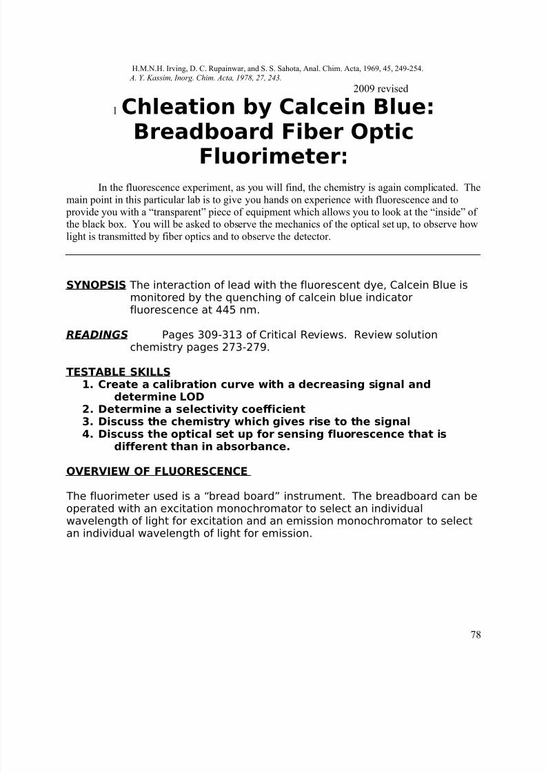
8/3/2019 2011 lab book V3


H.M.N.H. Irving, D. C. Rupainwar, and S. S. Sahota, Anal. Chim. Acta, 1969, 45, 249-254. A. Y. Kassim, Inorg. Chim. Acta, 1978, 27, 243.

2009 revised

1 Chleation by Calcein Blue:

Breadboard Fiber OpticFluorimeter:

In the fluorescence experiment, as you will find, the chemistry is again complicated. Themain point in this particular lab is to give you hands on experience with fluorescence and to provide you with a “transparent” piece of equipment which allows you to look at the “inside” of the black box. You will be asked to observe the mechanics of the optical set up, to observe howlight is transmitted by fiber optics and to observe the detector.

SYNOPSIS The interaction of lead with the fluorescent dye, Calcein Blue ismonitored by the quenching of calcein blue indicatorfluorescence at 445 nm.

READINGS Pages 309-313 of Critical Reviews. Review solutionchemistry pages 273-279.

TESTABLE SKILLS1. Create a calibration curve with a decreasing signal and

determine LOD

2. Determine a selectivity coefficient3. Discuss the chemistry which gives rise to the signal4. Discuss the optical set up for sensing fluorescence that is

different than in absorbance.

OVERVIEW OF FLUORESCENCE

The fluorimeter used is a “bread board” instrument. The breadboard can beoperated with an excitation monochromator to select an individualwavelength of light for excitation and an emission monochromator to selectan individual wavelength of light for emission.

78

8/3/2019 2011 lab book V3


The current set up (2009) uses a different set up with a 180o excitation to

emission angle.

The signal of the blank and samples may be contaminated by excitationwavelengths that reflect off the container interior. This can be reduced byplacing black electric tape on both the interior and exterior of the vial.Placing black tape on the interior could, however, result in crosscontamination. .

Calcein Blue Fluorescence Quenching by Lead.Calcein Blue is a molecule which contains two basic molecular units.

The ring structure is the optically active site of the molecule. The attached

79

8/3/2019 2011 lab book V3


chelating arm is the site which binds metal ions. The ring structure iscapable of intense absorbance and intense emission.

The signal is pH dependent because the absorption band at 320 (pH 6-8)moves to longer wavelengths near 370 when the –OH group becomesdeprotonated (pH 8-10). For our instrument we use the entire spectra forexcitation, so we will still see emission, however as the emission intensity isa function of the absorbance emission will vary with pH. As a result we mustcontrol the pH to a range of 6-8. This pH is also optimal because it keeps thebulk of lead in the divalent cationic form.

80

8/3/2019 2011 lab book V3


The emission is quenched with the addition of Pb2+. Most chemists wouldsuggest that quenching is the result of the heavy metal status of lead inwhich a local magnetic field caused by the density of electrons on leadenhances electron spin flip into the triplet state which has lower probabilityof emission. NMR studies suggest that quenching by lead is accomplished by

binding of lead to the phenolic OH preventing an excited state resonancestructure which leads to emission. In either case the selectivity of themethod is likely to be low.

Because the signal decreases with increasing Pb2+ the limit of detection iscalculated as

X X s L O D b l a n k b l a= − 3

81

8/3/2019 2011 lab book V3


SOLUTIONS

2M NaOAc (50 mL) + 2M HOAc (50 mL): pH ~∼ 5Stock 1000 ppm Pb, Cd0.01% aqueous solution of Calcein Blue (10 mL) (4-

methylumbelliferone-8-methylene-iminodiacetic acid)

Dissolve 4.6 mg CB in 10 mL buffer

The molarity of this solution is can be calculated from themolecular weight of the CB (321.29 g/mole)

Fluorimeter

To OperateTurn on Power Supply for Lamp.Unlock the output dial.

At same time: push in pre-adjust button and dial output dial to5.4 Amps.Release pre-adjust and lock output dial.Press Lamp start button until lamp fires.

PROCEDURE

1. Attach one of the “long” ends of the bifurcated fiber optic into thesource. Attach the other “long” end into the Ocean Optics detector.

2. Cover the joined end of the fiber optic bundle and observe the spectra.It should have a very low signal intensity.

3. Uncover the joined end of the fiber optic bundle and observe thespectra. The intensity of light observed is due to “pick up” of the lightfrom within the lab.

4. Cover a 20 dram vial inside and out with black electrical tape. Placeenough CB free solution (contains any other reagents such as buffersand salts but no CB) into the vial to cover the bottom. Cork the vialwith a cork that has a “hole” for the fiber optic tip. Place the fiberoptic near the top of the vial and observe the spectra. The light youobserve represents light reflected from the interior of the vial. Move

the fiber tip within the vial until you find a location that has the lowestreflected intensity. Mark that distance. You will make all of yourobservations at that tip distance within the vial.

5. Check the pH of a fresh solution of 10 mL CB. The pH should bebetween 6 and 8. Place the solution into the vial and take an emissionspectra using the software to integrate at various times. Choose your

82

8/3/2019 2011 lab book V3


times to increase by the square of N. (For example integrate for 4, 9,16, etc. s). Make at least three measurements of this blank reading.

6. Add Pb2+in increments and monitor the emission spectra at eachincrement. Increments begin with 25 uL, a second 25 uL, 50 uL, 100uL, then add by 100 uL until a total of 1000 uL have been added. Then

add 200 uL increments until a total of 2000 uL have been added. Thenadd 1000 uL for a total of 3000 uL.7. Repeat 5 & 6 for Cd2+

REPORT In addition to methods, materials and results, include thefollowing:

1. Describe the chemistry of the procedure.2. Map out in detail a method for the analysis of lead.3. What might be some serious problems with your method? (I.e.

interferences?, background from your soil sample?) I.E., what are the

effects of matrix in this method?4. What would be the estimated time involved in a single measurement?5. What is the probable structure of the fluorescing compound at

intermediate pH values? How does Pb2+ interact with it do reduce thefluorescence? Construct a reasonable chemical argument as to thesensitivity of the method to pH.

6. Would there be any problems with disposal of hazardous materials?7. How easy would you anticipate it be to instruct a technician on this

method?8. What are the figures of merit for this method.9. What is the selectivity of the method when compared to quenching by

Cd2+

?

1 Materials:

Playa Cesar et al Environmental Science Technology 2006, 40 917-923: Molecular and Quantitativeanalysis of metal ion binding to humic acids from sewage sludge and sludge amended soils by

fluorescence spectroscopy Deo, Sandhya and Hilary Arnold Godwin, Journal of the American Chemical Society 2000, 122, 174-175, A

selective Ratiometric Fluroescence Sensor for Pb 2+

83

8/3/2019 2011 lab book V3


1IR Determination of Pb bindingto EDTA

SYNOPSIS The binding of Pb to EDTA will be studied using the vibrationalchanges in EDTA when Pb is added. An FTIR instrument is used.

READINGS 279-285 on EDTA and 319-325 on vibrational spectroscopy inCritical Reviews

SuppliesKBr SlidesNujol OilMortar and Pestle

Glassware

One 30 mL beaker

CAUTIONS AND PROBLEMS This method is quite difficult because it relies on accurately bringing asolution chemistry down to a dry state. Lead EDTA has very differentconformations and structures in the wet and dry states. Samplepreparation must be performed with extreme care.

Solutions

These should be made up before this lab.

Combine 1.000 g (0.00342 moles) of Na-EDTA and 1.133 g (0.00342moles) of Pb(NO3)2 in 10 mL of water and adjust the pH with 0.6 M NaOH to apH 9-10 value under continuous stirring. Discontinue stirring as soon asthere is no solid material left and dry the sample at 80 oC for more than 3days.

Sample Preparation

Weigh out five 10 mg EDTA samples and to each of them add 0, 0.25,0.5, 0.75, and 1 stoichiometric molar amounts of EDTA-Pb complex. Grindthese separately to a fine paste on an Agate mortar about 15 minutes. Add1 to 2 drops mineral oil and grind again. Use a rubber policeman to transferthe paste/oil to KBr plate . Press between two plates to create a thin filmthat is almost translucent.

84

8/3/2019 2011 lab book V3


Experiment

1. Take a spectrum of Nujol by itself. Export the data.

For our FT instrument the data will be exported into a text file. To get it into

a form you can manipulate in excel you will need to import the data and delineate it into an Excel format. A. Go to Data/Get External Data/Import Text FileB. In the Import Text File command box indicate that the data is

delimited, and enter C. On the next command box indicate that the data is delimited by

commas and hit enter D. You should be able to simply hit finish, finish and find your data

imported into Excel in a readable format

2. Obtain a spectrum of pure EDTA in Nujol. Compare the peaks that youobserve to those listed in Table 27, p321 in Critical reviews.

3. Run each of the lead samples. Pay particular attention to the regionbetween 1500 and 1700 cm-1.

4. Overlay the different mole ratio spectrum.

REPORT: Report, in addition to materials, methods and results.

1. Why is the lead EDTA complex formed at pH 7? Give two separatereasons.

2. Why does the sample have to be ground to less than 2 µm particlesize?

I. Identify, with Table 27, page 321 in Critical Reviews, the majorabsorption bands of EDTA.

4. Can you observe the Pb-N band? Why or Why not? What would youneed to do to see this band?

5. Prepare a table which quantitates the decrease in the C=O band andthe increase in the C=O-Pb band. Is the decrease quantitative? Whatis the LOD?

6. Quantitate the effect of the increasing of co-added spectrums on theS/N of the spectrum. Plot the S/N as a function of square root of theco-added spectrum. Is the plot consistent with what you expect?

7. How does the k value for Pb-O compare to Pb-S?8. Discuss the use of EDTA has a chelation therapy for lead. What are

some of the pitfalls? How would you design a chelate to overcomethose pitfalls?

85

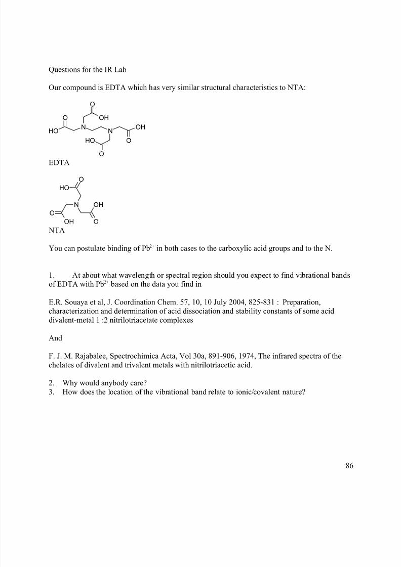
8/3/2019 2011 lab book V3


Questions for the IR Lab

Our compound is EDTA which has very similar structural characteristics to NTA:

O

OH

N

O

OHN OH

O OH

O

EDTA

N

O

OH O

OH

O

OH

NTA

You can postulate binding of Pb2+ in both cases to the carboxylic acid groups and to the N.

1. At about what wavelength or spectral region should you expect to find vibrational bandsof EDTA with Pb2+ based on the data you find in

E.R. Souaya et al, J. Coordination Chem. 57, 10, 10 July 2004, 825-831 : Preparation,characterization and determination of acid dissociation and stability constants of some aciddivalent-metal 1 :2 nitrilotriacetate complexes

And

F. J. M. Rajabalee, Spectrochimica Acta, Vol 30a, 891-906, 1974, The infrared spectra of thechelates of divalent and trivalent metals with nitrilotriacetic acid.

2. Why would anybody care?3. How does the location of the vibrational band relate to ionic/covalent nature?

86

8/3/2019 2011 lab book V3


NMR lead 207 .

SYNOPSIS The natural abundance of 207-Pb is determined by proton NMR from a

lead-EDTA chelate. The structure of binding of EDTA-Pb in solution isalso investigated.

READINGS Review all preceding labs on EDTA and Lead. Review labs on pH, Read section on EDTA and again EDTA and NMR (pages 325-329 in Critical Reviews), also read section in IR and EDTA:(pages319-325).

Caution This lab is extremely sensitive to the mole ratio of EDTA to Pb and tothe pH. The binding of lead to EDTA changes with pH, which changes

the linewidths so that resolution can be lost. Furthermore the207

Pbcoupling through the nitrogen depends on the half life of that bondwhich is also dependent upon the mole ratio and pH.

INSTRUMENTpH meterNMR (Varian EM 360A 60 MHz magnet coupled to an Elbit ATI series2000 FT console)

CHEMICALS TMS as a reference

D2OPb(NO3)2 Na2EDTASodium bicarbonateSodium carbonate

Buffer Preparation (pH 9.2)0.2 M Na2CO3 = 0.0212 g of anhydrous Na2CO3 in 1 mL of D2O0.2 M NaHCO3 = 0.0168 g of anhydrous NaHCO3 in 1 mL of D2O

Combine 0.46 ml of 0.2 M soidum bicarbonate with 0.04 mL of 0.2 M

sodium carbonate and dilute it with 0.5 ml of D2O.

Note: A better NMR spectrum resolution can be obtained by adjustingthe sample pH with dilute NaOD instead of using the buffer. However,the final volume (if needed) would have to be measured after the pH isadjusted. Also a small pH electrode would be needed.

87

8/3/2019 2011 lab book V3


Sample PreparationDry the powdered lead nitrate two hours at about 130 C to removewater.Dry the Na2EDTA-H2O 4 days at 100oC to remove water. The molecularweight of the dried EDTA is 336.2 g/mole.

Preparation of a 1:1 mole ratio EDTA/Pb.

0.0250 g Na2EDTA * 1 mole Na2EDTA/336.2 g = 7.437x10-5moleNa2EDTA7.437x10-5 mole Na2EDTA * 1 mole Pb(NO3)2/1mole Na2EDTA *####/1molePb(NO3)2

= 0.02463g Pb(NO3)2

1. Combining equal molar amounts of Na2EDTA (0.0250 g) and Pb(NO3)2

(0.02463g) in a Wheaton 4 ml sample vial.

2. Add 0.8 mL of D2O. A white precipitate will be formed. Add NaOD.3. Sonicate (about 5 min.) at room temperature to speed up the EDTA/Pbcomplex formation.

4. As soon as there was no solid material left in the vial the sample wastransferred to an NMR tube.

5. Perform all references against water.

Note to instructor: Samples of the pure EDTA at this buffer should beobtained also.

Students may wish to observe the change in the EDTA with pH by

changing the bicarbonate buffer.Students may wish to observe the change in the spectra with different mole ratios of lead to EDTA. The best experiment is to increase theamount of lead present.

METHOD

1. Obtain an NMR spectra for each of the solutions2. On the spectra acquire the peak area separately for each of the

doublet peaks and the central peak.

REPORT

1. Identify the major peaks in your NMR spectrum. (Recall that the peakheights correlate with the number of protons.)

2. Why don't the ethylenic protons shift to the same extent as the acetateprotons?

88

8/3/2019 2011 lab book V3


3. Would you expect differences in this spectrum and that of Zn-EDTA?Do you think you could resolve the two species if they were presentsimulataneously in your sample?

4. Compute the % relative abundance of lead 207from the side bands.Does your value compare well with the published data?

5. Would you be able to tell the difference between a lead ore from twodifferent mines with this method. (Calculate the std. deviation andcompare it to the std. Deviation associated with variation in207-Pb.

6. Can you think of a use for this method with respect to the analyticalissues faced in the lead-environmental controversy?

7. Why can't we perform the analysis in water?8. Compute the % natural abundance of 207-Pb.9. Measure and identify the chemical shift associated with the protons in

EDTA in each of the 5 spectra.10. Measure the spin-spin coupling constant, J(Pb-H), for the 207Pb deriveddoublet.

11. Measure the peak width at half height for the doublet peaks associatedwith 207Pb in each spectra.12 From the peak width calculate the lifetime of the complex.13. Plot the lifetime of the complex as a function of mole fraction of thecomplex.14. What importance might the lifetime of the chelate-metal complex have

on use of the chelate in lead poisoning therapy?15. Are there any problems with disposal of hazardous materials?16. How easy would it be to instruct a technician on this method?

1 Articles Alicia Glatfelter et al The Analyst. 2006 131, 1207-1209: Quantitative

determination of lead in a mixture of lead(II) halide using solid-state

207Pb NMR spectroscopy.

Additional questions for NMR based on the three articles:

1. Rabenstein, Nuclear Magnetic Resonance Studies of Solution chemistry of Metal Complexes.

2. Dowd,: The 1H NMR structure of bo9vine Pb2+ osteocalcin and implications for lead

toxicity; Biochimica et Biophysica Acta

3 .Glatfelter, Quantitative Determination of Lead in Mixtures of Lead (II) Halides Using Solid-

State 207 Pb NMR spectroscopy; The Analyst;

89

8/3/2019 2011 lab book V3


Questions1. Look at Figure 1 of Rabenstein. Qualitatively describe the different shapes of the NMR peak in Figure 1. How do they change with the concentration of excess NTA added to the solution?Do you see any similarities in peak shape when looking at your PbEDTA NMR?

2. How does Rabenstein explain those peak differences?

3. How might a study of PbEDTA by NMR contribute to an understanding of its use as a pharmacologic agent?

4. Look next at Dowd’s article. Does this article relay on the 207-Pb coupling to proton NMR?Or does the information that the authors obtain rely on the changes in conformation and changesin electron density driven by any type of isotope? Why does Dowd choose Ca2+ as acomparison for this article?

5. (See Glatfelter). Where is the signal found in Glatfelter’s study of 207Pb directly compared

to the proton coupled effect of 207Pb on EDTA?

6. In Glatfelter’s article compare the instrumental parameters used to those used in your experiment, specifically MHz of the instrument, co-added spectra, reference compound, pluswidth, and relaxation delay. Are there major differences? If so speculate why there might bemajor differences.

7. What is the total time required for each spectra? How does that compare to your PbEDTAexperiment? Why should there be such a difference?

90

8/3/2019 2011 lab book V3


Circular Dichroism: Binding of Lead to Osteocalcein

R. Andrew Atkinson et al European Journal of biochemistry 232, 515-521,1995. Conformational studies of osteocalcin in Solution

T. L. Dowd et al biochimica et Bioophysica Acta 1784 2007 1534-1545, The1H NM strcture of bovine Pb2+ osteocaclin and implications for lead toxicity

T. L. Dowd et al The effect of Pb2+ on the structure of hydroxyapatite and properties of osteocaclin Biochimica et biophysica Acta 1535 2001 153-163

91

8/3/2019 2011 lab book V3


Revised 1/2011 Mary Van Osptal

PbS/Ag2S Based Ion SelectiveElectrode

Pb-EDTA Potentiometric Titration.Potentiometric titrations are one of the most accurate methods to

determine endpoints (the point at which the lead is consumed completely byEDTA). However, a titration must be done under very specific conditions toalleviate any problems due to pH, precipitate, or effects of the ISE. Twoimportant aspects to understand about ISE titrations are the effects of protonconcentration, and the formation of Pb(OH)2. For the ISE to detect all thelead, then it cannot be “held up” by the competitors. If the instrumentalmethod is sampling only the liquid phase of the system then the precipitatewill not be measured and a negative determinate error is imparted to the

entire analytical scheme.

SYNOPSIS: This lab is designed to illustrate the role of pH in detecting thepresence of lead. Students will monitor the lead concentration and pH insolution through a titration with EDTA using a lead ion selective electrode(ISE). Key concepts in this lab will be the effective ionic strength on themeasurements, ion selective electrodes, and calculation of leadconcentration during titration. This lab will also give further practice on theuse of spreadsheet calculations and manipulations.

READINGS Read pages 273-276 in Critical Reviews on solution

soluble chelates and pages 291-293 on ion selective electrodes.An attached article illustrates the design, construction, andfunction of a polymer based ISE based on chemistry similar tothe dithizone UV-Vis lab.

Testable Skills 1. Construct alpha plots given the appropriate information.2. Create a calibration curve3. Calculate concentration of lead at each point in titration curve.4. List/Define limits and advantages of the method5. Explain the chemistry which results in a signal

PRE-LABBefore coming to lab the student should1. Calculate an alpha fraction plot vs pH for lead.2. Use literature data for Pb in chloride system to calculate sequentialformation constants.Complex equilibria and calculations of formation constants frompotentiometric data

92

8/3/2019 2011 lab book V3


A metal ion can bind to a ligand (L=Cl-, CN-, OH-, etc.) in sequential steps.Reaction Constant Conc in terms of stepwise and overall

formation constants[1] M + L = ML K 1 [ML] = K 1[M][L][2] ML + L = ML2 K 2 [ML2] = K 2[ML][L] = K 1K 2[M][L]2 = 2[M][L]2

[3] ML2 + L = ML3 K 3 [ML3] = K 3[ML2][L] = K 1K 2K 3[M][L]3

=3[M][L]

3

[n] ML(n-1) + L = MLn K n [MLn] = K n[ML(n-1)][L] = K 1K 2...K n[M][L]n = n[M][L]n

Each reaction has been solved for the equilibrium concentration of theappropriate species in terms of the sequential or step-wise equilibriumconstants, K i, and in terms of the overall equilibrium constant,i.A mass balance for all forms of the metal is written as:CM = [M] + [ML] + [ML2] + [ML3] ...+ [MLn]

(1)which can be replaced by the concentration terms shown above:

CM = [M] + K 1[M][L] + 2[M][L]2 + 3[M][L]3 + ..... n[M][L]n

(2)We can define a denominator “D” as:

D = CM/[M] = 1 + K 1[L] + 2[L]2 + 3[L]3 + .....n[L]n

(3) To calculate the fraction of the total amount of metal in each form we definethe “alpha” fractions:0 = [M]/CM = 1/D (4)1 = [ML]/CM = K 1[M][L]/CM = K 1[L]/D

(5)2 = [ML2]/CM = 2[M][L]2/CM = 2[L]2/D (6)3 = [ML3]/CM = 3[M][L]3/CM = 3[L]3/D (7)n = [Mln]/CM = n[M][L]n/CM = n[L]n/D (8)

Typically the alpha fractions are plotted against the ligand concentration. This allows one to see what form of the metal is most prevalent at any givenligand concentration.

93

8/3/2019 2011 lab book V3


1.2

o

n

Figure 1 Alpha Plot of lead speciation as a function of pH

Figure 1 is a plot of only two the lead species, Pb2+, and Pb(OH)+, as afunction of pH.. You will make a full plot of all alpha fractions using aspreadsheet.

Pb/Hydroxide alpha plotUsing a spreadsheet create and alpha plot fraction for lead using thefollowing constants:logK 1 = 7.82Log2 = 10.88Log3 = 13.94Log4 = 16.30 This is easiest done with the following set upColumn A: pH values from 1 to 14 in some small incrementColumn B: [OH-] values corresponding to the pHColumn C: D = 1 + K 1[OH-] + 2[OH-]2 + 3[OH-]3 + .....n[OH-]n

Column D: 0 = 1/DColumn E: 1 = K 1[OH-]/DColumn F: 2=2[OH-]2/DColumn G: 3=3[OH-]3/DColumn H: 4=4[OH-]4/DHere is a picture of my spread sheet:

94

8/3/2019 2011 lab book V3


Ion Selective ElectrodesIn potentiometric methods the selective charge distribution across amembrane is monitored as a potential. Charge distribution arise due to twoprocesses, interfacial equilibria, and membrane mobility of the ion (seeFigure 2).

95

8/3/2019 2011 lab book V3


Figure 2: Diagram of solid phase and solution phase processes for the leadion selective electrode.

In Figure 2 there is a mobility of Ag+ ions through a mixed crystal of PbS/Ag2Sthat is controlled by solubility of the two crystals and by the bulk solutionconcentration. If on the interior of the crystal is a fixed solution of silver, and

if Ag+

moves across the crystal in response to a concentration gradient, thencharge will be differentially displaced due to movement of cations but not of anions. Since voltage is defined as the amount of charge, Q, stored over thetotal possible stored charge (capacitance), C:

V Q

C = (9)

a voltage develops which can be measured across the crystal. The chargestored depends upon the mobility of Ag+ within the crystal.

When all goes well and the silver ion activity is controlled by lead ionactivity in solution then the response of the electrode to the lead ionactivity is given by the Nikolsky equation:

( ) E c o n st R T z F

a k ai

i i j j

z i z j= + +t a n . l o g/

2 3 0 3 (10)

where E is the measured voltage (V), the constant relates to the internalfilling solution, R is the natural gas constant, T is the temperature in Kelvin, Fis Faraday's constant, zi is the valence of the ion, i, (here Pb2+) measured,and ai is the activity of the ion measured. Temperature is clearly important:

96

Pb2+

S2-

Ag+

Pb2+

S2-Pb2+

Pb2+

S2-

S2-

Ag+

S2-

S2-

S2-

Pb2+

Ag+

S2-

H+

Cl-

SO42-

Pb2+

S2-

Ag+

Pb2+

S2-Pb2+

Pb2+

S2-

S2-

Ag+

S2-

S2-

S2-

Pb2+

Ag+

S2-

H+

Cl-

SO42-

8/3/2019 2011 lab book V3


Assuming room temperature and combining constants we find:

( ) E c o n st m V

za k a

i

i i j j

z z j= + +t a n.

l o g /5 91 6

1 (11)

The activity of the ion is related to the concentration of the ion via theactivity coefficient:a f C i i i= (12)

The activity coefficient is a function of the ionic strength, I, of the solution:

l o g.

f z I

I z =

−+

0 5 1

1

2

(13)

where the ionic strength of a solution is affected the concentrations of all of the ions and their charge, z.

I C zi i= ∑1

22 (14)

Clearly equation 11 indicates that the voltage measurement will behighly dependent upon the ionic strength of the solution, therefore it is oftensuggested that an ionic strength buffer be used.

Equation 11 also indicates that the electrode may respond directly toother ions which are mobile within the solid state membrane. This particulartype of lead ion selective electrode responds directly to protons which arealso mobile within the crystal lattice. In Figure 3 (from the Orion Lead IonSelective Electrode manual) it can be observed that at pH 8 it is theoreticallypossible to measure 10-6 M lead ion, while at pH 2 the limit of detection isapproached at ~10-3 M lead ion.

97

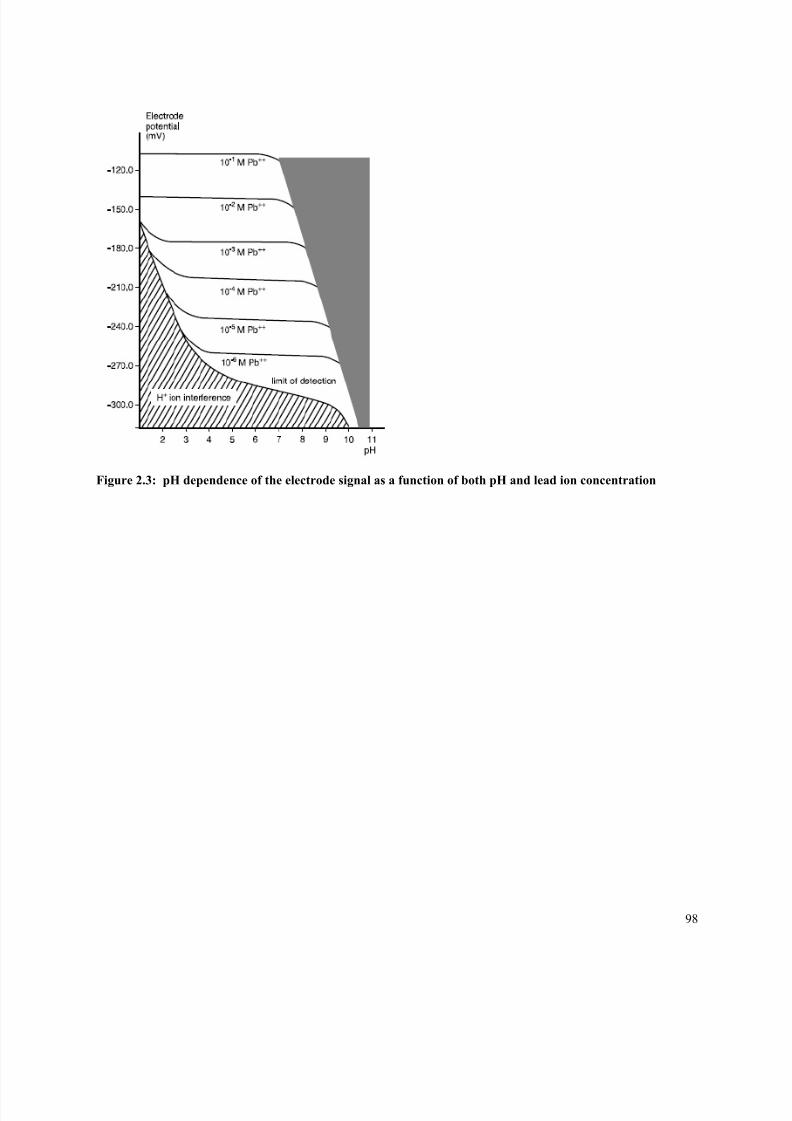
8/3/2019 2011 lab book V3


Figure 2.3: pH dependence of the electrode signal as a function of both pH and lead ion concentration

98

8/3/2019 2011 lab book V3


GLASSWAREBeakersVolumetric pipet (10mL)

EQUIPMENT

Lead Ion selective electrodeSCE electrode (if needed)Voltmeter (connected to computer)Stir bar/Stir platepH meter (to check pH) Thermometer (to measure temperature)Calibrated pipets (100µL to 1000µL)

SOLUTIONS0.001M Pb2+ solution (from 1000ppm stock solution) (Pb(NO3)2) (MW =331.22g/mol)

0.01M EDTA solution (Na2EDTA)1M NaNO3 solution (Ionic Strength Adjustor)Methanol with Formaldehyde

Add three drops of 36% formaldehyde to 1,000 mL reagent grademethanol. What is the purpose of this reagent? (see yourarticles!!!)

Buffer – 0.1M acetate pH 5 buffer0.1 NH4Cl/NH3 pH 10 buffer0.1 M NaOH, HNO3 to adjust pH

CAUTIONS AND PROBLEMS The ion selective electrode responds to free sulfide, to lead,and to pH effects. As a consequence the pH must not dropbelow pH 4.5, nor should it exceed pH 8. When the pH exceedsthese limits the calibration curve obtained will not be correct.The method is further complicated by the slow equilibrationtime required for the electrode.

PROCEDURE1. Connect leads of the Saturated Calomel Electrode and Pb ISE to

voltmeter. Check which way you connect them and continue to

connect in exactly the same manner in any subsequent experiments,otherwise your reading will change from positive to negative.

2. If Pb electrode is dirty, polish gently on polishing strips. (See

instructions in your Appendix for the Orion PbS ISE).

3. Rinse electrodes, blot dry.99

8/3/2019 2011 lab book V3


4. Test slope of electrode

a. Place the electrode in a solution of with 0.5mL 1000ppm Pb and

5mL methanol, record potential

b. Add 5mL more to solution and record potentialc. The change in potential for a decade (exponential) should be

between 25-30mV.

A. Temporal response and calibration curves5. Measure each of the standard solutions for both pH and mV. You

may have to wait up to or more than ½ hour for the voltage tostabilize. The computer will monitor you’re your potential every5 seconds; however you must keep an eye on the pH. Monitorthe pH and mV at 1 minute intervals. Record the voltage and

time as you are doing this. Your data may look like this:Milliseconds pH mV

750 7.81 -196.8

780 7.89 -196.1

810 7.91 -193.9

840 7.89 -191.6

870 7.91 -190

900 7.9 -188.5

930 7.91 -187.2

960 7.9 -186.3

990 7.9 -185.5

1020 7.9 -185.2

1050 7.9 -184.5

1080 7.9 -184.1

1110 7.89 -183.8

1140 7.9 -183.4

1170 7.88 -182.9

-184

-182

100

8/3/2019 2011 lab book V3


6. Notice that there is a definite time required to reach equilibriumat the electrode surface. You will want to monitor the time (plotit!) and wait for a stable reading before you add more material toyour solution. When the change in mV is less than 0.5 mVbetween minutes readings you may be near an equilibrium. The

best way to tell if you have come to equilibrium is to plot in labas you acquire the data the mV reading vs time. The pH shouldbe identical for each of the standards and should be 4.5otherwise you will not get a calibration curve when you are done.

7. You will need to take the mV reading of one of the standardsat least three times in order to determine an experimentalstandard deviation necessary for your LOD calculation.

8. You will perform a calibration using the same solution as in the

titration. Make up several standards. How many standards should you

make up, and at what concentrations? Look at the potential vs. pH plot

found in this lab and think about the pHs at which the electrode best

performs.

9. Wait for the potential to stabilize and record. Make a calibration curve.

Plot potential reading (mV) vs. the log[Pb concentration]. Be sure to

allow for dilution and for the fact that the response is with the

logarithm of concentration. Determine your equation, and find the

slope. What value should this be?

mV = A + Blog[Pb2+]B. Pb-EDTA Titration

10. Place electrode, pH meter, stir bar into a 100mL beaker of

a. 10mL 0.001M Pb2+ solution

b. 10mL methanol

c. 2mL buffer

d. 0.25mL ISA

11. You have two choices for buffer, a 0.10M acetate buffer at about

pH 5, and a phosphate buffer at pH 10. Which buffer do you think you

should use and how can you figure that out? Think about pH, the alpha

plot of Pb(OH)2

12. Once you have determined your best buffer, Record initial pH

and potential. It may take 10-20 minutes for it to stabilize. Be patient!

101

8/3/2019 2011 lab book V3


13. Add 100uL of 0.01M EDTA at a time, record the potential once it

stabilizes.

14. Determine the endpoint before you come to lab so you know

what to expect it.

15. Take data until the endpoint and just a few points past (about 5).

This may be difficult. After the endpoint, how much lead is left in

solution? What is the ISE detecting now? If the electrode potential

starts to change direction, what do you think is happening? What may

the excess EDTA be attracted to in the electrode?

16. It may be helpful to graph this in excel as the titration goes on, it

will show you if you are getting a curve.

17. Calculate the concentration of lead in each step. Make sure to

compare this to an expected titration curve (found in Ch. 14 of Harris

Quant Chemical Analysis).

18. To show your final titration curve, please provide a curve with pM

(Pb2+) vs. EDTA added and another with potential vs. EDTA added.

B. Estimate the selectivity coefficient for the Pb ISE for H+ usingthe fixed interference method (FIM) in which the fixed interferenceis 0.003162 M H+ (pH 2.5). Your calibration curves may look like this:

102

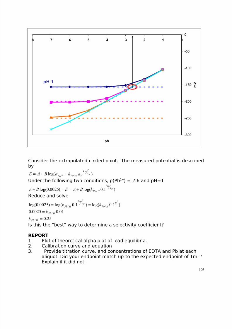
8/3/2019 2011 lab book V3


Consider the extrapolated circled point. The measured potential is describedby

)log( /2H

Pb

z

z

H H Pb Pb ak a B A E ++= +

Under the following two conditions, p(Pb2+) = 2.6 and pH=1

)1.0log()0025.0log( / H

Pb

z

z

H Pbk B A E B A +==+

Reduce and solve

25.0

01.00025.0

)1.0log()1.0log()0025.0log(

/

/

12

//

==

==

H Pb

H Pb

H Pb

z z

H Pb

k

k

k k H

Pb

Is this the “best” way to determine a selectivity coefficient?

REPORT1. Plot of theoretical alpha plot of lead equilibria.2. Calibration curve and equation3. Provide titration curve, and concentrations of EDTA and Pb at each

aliquot. Did your endpoint match up to the expected endpoint of 1mL?Explain if it did not.

103

-300

-250

-200

-150

-100

-50

0

012345678

pM

m VpH 1

8/3/2019 2011 lab book V3


4. Why did we use NaNO3 instead of NaCl for the ionic strength buffer?5. Why did we check to make sure that the solutions had a pH<5 for the

calibration curve?7. What is the purpose of the added methanol/formaldehyde? Hint:

Something about the chemistry of S in air.

8. Why does there seem to be a time response to the mV readings? Whatis the response time? Explain what is happening at the electrode interface. 9. What buffer did you choose and why? Describe any observations that

occurred with the buffers?10. Why does the pH drop as you add more EDTA? Think about the

reaction happening between EDTA and Pb.11. What implications does this chemistry have for lead analysis?12. What implications does this chemistry have for lead in the pipes toyour household? (Hint think about what pH your tap water is).13. Where might this technique be useful, and where might it not be usefuldue to limitations you experienced in lab?

Your T.A. will chose questions from the following for you to focuson.

REPORT (Remember – write an essay which weaves together thequestions – do not simply answer the questions in sequence). Youmay find some questions are irrelevant or you may find that youhave additional questions you wish to explore.

1. Plot of theoretical alpha plot of lead equilibria.2. Does your calibration curve for the lead ISE at pH 6 have the “right”

slope? Why or why not?

3. Does your calibration curve for the lead ISE at pH 2.5 have the “right”slope? Why or why not?

4. Why did we use NaClO4 instead of NaCl for the ionic strength buffer?5. Why did we check to make sure that the solutions had a pH<5 for the

calibration curve?

Question 6 relates to the article: Michael L. Clay and Vaneica Y. Young, Anal. Chem., 1993,65, 1094-1099, Corrosion of Lead Ion Selective Electrode Membranes: Effect of White

Light.

6. What information, inferences, hints, does this article give us about the procedure

recommended by the Pb ISE electrode and incorporated into the instructions of our lab?

Questions 7-9 relate to the article: Leo Lehrman: Studies in the precipitation of copper and tin groups using hydrogen sulfide.

7. Leo Lehrman, article from the 1930s, indicates in Part I of his article that there are chemicalinferences (GIGO alert: Garbage In = Garbage Out) complicating the analysis of lead by

104

8/3/2019 2011 lab book V3


sulfide precipitation. What are those complications? What causes on of those complicationsfor the method outlined by Lehrman?

8. Did Lehrman give a LOD? If so, what was it and how did he define it? Did he shown anycalibration curve? If so, what was the linear range?

9. How was Lehrman’s method made selective for lead compared to cadmium?

Questions 10-12 relate to the article: Pekka Sten and Willis Forsling , Colloids and Surfaces,172 (2000) 7-31: Precipitation of lead sulfide for surface chemical studies.

10. Sten precipitates Pb(NO3)2 by S2- while monitoring Pb2+ with an ISE. What is the

composition of the Pb ISE Orion 94-82 electrode that he uses?

11. How do the authors pinpoint the exact end point of the titration?

12. What is the effect of the time (slow or rapid) of the S

2-

addition on the ISE reading? Isthat effect due to the bulk solution reaction

Pb2+(aq)+S2−(aq)⇔PbS(

or to rates of reactions at the surface of the electrode?

Questions 13-16 relate to the article: F. C. Guthrie and J. T. Nance, J. Appl. Chem., I,March, 1951, 109: Determination of Lead as basic lead chromate and its application to the separation of lead from silver

13. Guthrie and Nance choose to determine Pb2+ by CrO42-. They identify several

interferences, which compromise the results. What are they?

14. Do they give a calibration curve?

15. Do they give an LOD? If so, what is it and how was it determined?

16. What is the response time that you measure in your experiment? In answering this question be sure to specify what concentration you are measuring the response time at. Will this makea difference?

Questions 17-20 relate to the article: K. Shipgun, O. V. Basanova, and Yu. A. Zolotov,

Sensors and Actuators B 10 (1992) 15-20, Performance of solid-membrane cation-selectiveelectrodes for flow-injection potentiometry.

17. This article addresses a feature that your lab calls attention to which is the rise time. How dothe authors define and measure rise time? How is that the same or different than the rise timeas defined in your S/N lab?

105

8/3/2019 2011 lab book V3


18. Were the authors able to determine the cause of the dynamic response time to your satisfaction?

19. Do they give LOD for their method? If so how do they determine it?

20. Do they give a selectivity coefficient for their method? Which ions interfere the most? Howdo their values for Pb/H compare with the value you calculate?

Question 21 relates to the following articles:

Maria Fouskaki and Nikolas A. Chaniotakis, Anal. Chem. 2005, 77, 1780-1784: Thick

membrane, solid contact ion selective electrode for the detection of lead at picomolar levels.

Satsuo Kamata and Kazuhiro Onoyama, Anal. Chem. 1991, 63, 1295-1298, Lead-Selective

Membrane Electrode using methylene bis(diisobutyldithiocarbamate) neutral carrier

Warren L. Erdahl, Clifford J. Chapman, Richard W. Taylor and Douglas R. Pfeiffer , TheJournal of Biological Chemistry, 275, 10, 2000, 7071-7079: Ionomycin, a carboxylic acid ionophore, transports Pb2+ with High selectivity

Wei-Jun Zhang, Chun-Yan LI, Xiao-Bing Zhang, and Zhen Jin, Analytical Letters, 40,1023-1035, 2007, Synthesis of an Amide-Linked diporphyrin Xanthene as a neutral carrier for Lead(II)-sensitive electrode

Langxing Chen, Jia Zhang, Wenfeng Zhao, Xiwen He, Yu Liu, Journal of ElectroanalyticalChemistry, 589 (2006) 106-111, Double-armed calyx[4]arene amide derivatives as ionophores for lead ion-selective electrodes

21. For the five articles above find the following information if available:a. What is the LOD and how was it defined?b. What is the response time?c. Were selectivity coefficients measured, and if so, against what ions?

d. Is a value of S/N given?e. These articles were chosen to illustrate the fact that the response tolead is induced by complexation of the ion by some reagent. Find the5 compounds used to induce selectivity to lead and include an imageof the compounds. Some useful sites for finding structures areChemIDPlus or NISTbook . Do they have any functional features incommon?

Questions 22-24 relate to the optional section of the lab

22.. (Optional) Compare your experimental alpha plot to your theoretical lead vs pH alpha plot. Do the plots match? Why or why not?23. What implications does this chemistry have for lead analysis?24. What implications does this c hemistry have for lead in the pipes to your household?

(Hint think about what pH your tap water is).

106

http://chem.sis.nlm.nih.gov/chemidplus/

http://webbook.nist.gov/chemistry/

http://chem.sis.nlm.nih.gov/chemidplus/

http://webbook.nist.gov/chemistry/

8/3/2019 2011 lab book V3


1

1 Anodic Stripping Voltammetry:

Formation of Metallic LeadSYNOPSIS Lead is reduced to metallic lead and concentrated into the small

volume of the mercury drop. After a set concentration period thelead in the drop is monitored by it's enhanced oxidation peak. The limit of detection can be adjusted by the concentrating time.Contaminate metals do not interfere because of the potentialdependence of the method. Organics in the matrix may affectthe mercury drop stability, since the surface tension of themercury drop is affected by adsorbates and by the saltconcentration in the solution. A standard addition method will be

used. (1

,2

,3

). The solution conditions can be manipulated tochemically resolve the Pb from the Sn peak.

READINGS pages 285-291 in Critical Reviews. Three articles are attached. The first illustrates chemical methods of resolving Pb from Cdusing Br complexation. The second article discusses the effect of Br on inducing Pb adsorption to Hg surfaces. The third articlegives a method for lead analysis in blood by use of a mercuryplated microelectrode.

Modulating Potentials to Achieve Resolution

To resolve Pb2+ and Sn2+ in the anodic stripping lab the potential associated with stripping thelead in the presence of a chelate must be calculated as compared to stripping tin. The basic ideais a LeChatlier’s principle:

Pb ⇆ Pb2+ + 2e + xL ⇆ PbL + PbL2 + PbL3 +......

By adding the ligand to the solution the reaction is shifted to the right (oxidation).

In electrochemistry reactions are always written as reduction reactions:

Pb2+ + 2e ⇆ Pb Eo pb

[ ] [ ]++ ==−=22

1log

059.0ln

Pbn

V E

Pb

Pb

nF

RT E E

Pb

o

Pbequil

107

8/3/2019 2011 lab book V3


To solve this equation we must make use of our strategy used during the alpha fraction plots:

[ ] [ ]2

2 PbL PbL Pb Pb

total ++=

+

Where L is some ligand like chloride or bromide or EDTAwhich can be written as:

[ ] [ ][ ] [ ][ ] [ ][ ] ....32123

2212

21

2 +++==++++ L Pb K K K L Pb K K L Pb K Pb Pb f f f f f f total

This is equation can be reduced to:

[ ][ ] [ ] [ ]

total

f f f f f f

Pb

L K K K L K K L K

Pb

3

123

2

121

2

11 +++=+

Finally our equation for the reduction of lead becomes:

Pb2+total + 2e ⇆ Pb

and the Nernst equation becomes:

[ ] [ ] [ ]

+++

−=total

f f f f f f o

Pb

L K K K L K K L K

n E E

3

123

2

1211log

0591.0

Which in turn becomes

[ ] [ ] [ ]( )

−

+++−=

total

f f f f f f

o

Pbn L K K K L K K L K

n E E

1log

0591.01log

0591.0 3

123

2

121

Or

total

o

Pbn E E

1

log

0591.0'

−=

From the above you can easily set up an excel sheet to see what would be the potential of lead vstin reduction as a function of the concentration of some ligand.

The citrate solution system will be more complicated because it will depend upon pH and thedeprotonation of the acid.

For chloride in the spread sheet set up column one as pL (-log[L]). The second column is then[L] (=10^(-a#)). The third column then can be the apparent formal potential for lead and the

fourth column the apparent formal potential for tin.

One only needs to set up a few rows at the top of the spread sheet for the appropriate constantsfor the formation of the ligand/metal species.

108

8/3/2019 2011 lab book V3


GLASSWARE 2 4 neck flasks1 L volumetric flask50 mL volumetric500 mL volumetric

SOLUTIONS1. “Blank” Buffer = 1 L of (0.12 HCl + 10 mM NaCl)

Conc. HCl = 12.1 M, so 10 mL conc. HCl/1L = 0.12 M. For this a graduatedcylinder is sufficient.

NaCl

M L g

mole Xg 01.0

144.58

1=

×

×

X = 0.5844 g500 mL of 0.1 mM HgCl2 in 0.12 M HCl

mM L g

mole Xg 1.0

5.05.271

1=

×

×

X = 13.575 mg2. 1000 ppm Pb stock solution

1000 ppm Cd stock solution = 1 g Cd/103g soln = 1 g Cd/L

( ) L

Cd g

LCdCl g

Cd g CdCl Xg

)(1

1

1

)(3.183

)(4.112

2

2=××

X = 2.03 g/L or 0.2g / 100mL

PROCEDURES

Deposit Mercury Film

1. Purge 30 mL of your mercury solution for 3 minutes with N2 to remove O2.

2. While the solution is purging polish your carbon electrode (gently!) with alumina andrinse with large amounts of D.I. water. Look at the surface under a microscope.

3. Pull the nitrogen out and cap tightly.4. Connect up leads. The carbon electrode is the working (WE) electrode, the SCE is the

reference (RE) electrode and the small stub of Pt is the counter (CE) electrode. You mayhave to connect the ground wire also.

5. Turn on stir bar. The bottom of the flask is curved so turn past "2" until the bar is freelymoving and then back down to "2".

6. Deposit mercury by sitting at -900 mV relative to the resting potential for 3 minutes. Theresting potential can be found under Cyclic Voltammetry (CV) option of the softwaremenu. Note that if it is unstable the circuit probably is not closed (the electrodes are not

connected properly). Check the WE surface under a microscope again. You shouldobserve a gray mercury film on the surface.

Anodic Stripping Voltammetry: Optimization

1. Purge 30 mL of blank solution (no Hg in the solution).2. Place mercury film carbon electrode in the purged solution.

109

8/3/2019 2011 lab book V3


3. Start the stirrer.4. Using a pipette inject 15 μL of 1000 ppm Pb solution. Adjust the initial and the final

potentials to -900 mV and +100mV relative to the resting potential, respectively. Depositthe lead for 15s. Turn off the stirrer for at least 15 s (rest time). Take a scan and plot,determine currents. If you are using ASV option the stirrer should be turned off well

before the deposition time is up. In this mode the software will automatically take a scanfor you. Anodic stripping of Pb should be expected at ~ -500mV. If there is an additional peak towards the final potential (positive end) it is due to anodic stripping of the mercuryfilm. Thus, it should be avoided.

5. Repeat scan three times. You will have to do it in CV mode and extract the necessarydata from it since the software sweeps the potential in cycles from initial to final, andfrom final to initial, and etc.

6. Change deposition time to 30 s, 60s, and 120 s, and record corresponding scans. Themethod that you employ to find the current, i.e. scanning, should stay consistentthroughout the experiment since successive scans will not necessarily produce the samedata. For example, if you have used the first scan then you should use only the first scan

obtained after each additional deposition.7. Choose the most appropriate deposition time and create a standard curve. It should bemade with an internal calibration by adding 0.5 mL of stock Cd (1000 ppm) to thesolution and adding successive amounts of 15 μL Pb. You should have at least 5 points.

8. When you are done with the standard addition, add enough Pb to have a total addition of 1 mL.

Samples

1. Take 25 mL of your sample and add 15 mL of the matrixmodifier.

2. Deaerate, and obtain ASV under same conditions as for thestandard curve.

REPORT In addition to material, methods and results, include:

1. Use the std. add. method data to calculate the LOD, LOQ, linear range,and r value of your standard curve for this method.

2. How does the LOD of this method compare with the value necessary tomeasure the soil samples?

3. What is the relative standard deviation for your measurement of 3 ppmPb. How does it compare with previous measurements?

4. What constitutes a blank in this procedure? What are the sources of error embodied in the standard deviation of the blank? How would youdetermine the source of error attributed solely to the ASV?

5. How does sample matrix affect your results?6. What was the estimated time for turn around in samples?7. Are there any problems with disposal of hazardous materials?8. How easy would it be to instruct a technician on this method?

110

8/3/2019 2011 lab book V3


9. How easy would it be to construct a paper trail for this method?10. How does preconcentration time (deposition) scale with the signal?11. Which metals will interfere the most with Pb? How well resolved was

the Cd peak from the Pb peak?12. How was the baseline handled in this experiment?

13. What is the advantage of the standard addition method?14. What is the point of the N2 purge?15. Why does the ASV experiment show a peak? Why does the peak

current decay to background?16. What is the point of the added HCl and NaCl?17. Calculate the resolution of the Pb and Cd peaks.

Additional Questions for ASV based on the four articles

1.Brand: the Silver Electrode in Square-Wave Anodic Stripping voltammetry. Determination of

Pb2+ without Removal of Oxygen

2. Feldman: Determination of Lead in Blood by Square Wave Anodic Stripping voltammetry at

a Carbon Disk Ultramicroelectrode

3. Liu: Indium as Internal Standard in Square Wave Anodic Stripping Analysis of Lead in

Blood with Microelectrode Arrays

4. Zelic: Bromide induced adsorption of lead ions on mercury electrodes

Questions:

1. In Brand’s article why does he/she want to use a silver electrode instead of the electrode thatwe used? What detection limit does he/she report? What problems arise from use of the silver compared to our mercury film? The author reports two measures for sensitivity. What are theyand how are they different? Is the Pb peak well resolved from the copper peak?

2. In Feldman’s article why does he/she want to use a carbon electrode instead of the electrodethat we used? What is the major analytical problem that the authors address to achieve goodresults in this paper? Do they report their S/N; LOD; etc?

3. What electrode surface are they in Liu’s article using? Is it modified with Hg? In Figure 1In is not baseline resolved from Pb. How do they ultimately manage to achieve resolution? Theauthors use In as an internal standard. What is an internal standard and why have they decided itneeds to be added to the analysis of lead in blood? Figure 3 shows the raw data for thecalibration curve using 100 ppb In as an internal standard. How do the authors use the data tocreate a calibration curve based on the internal standard and the lead concentration?

111

8/3/2019 2011 lab book V3


4. In the preceding article by Liu the In and Pb peaks are resolved by judicious Br additions. Inthe article by Zelic the reason for peak differences are investigated. What do they ultimatelyconclude about the use of PbBr2; PbCl2; and PbI2?

1 Flame Atomic Absorption Spectrometry

SYNOPSIS Lead in liquid samples is aspirated into a flame to dry andatomize the sample. The atom vapor is probed with amonochromatic beam of light specific for the excitation of valence electrons in Pb. Depending on the instrument used,automatic background correction is performed.

READINGSRead pages 293-301 in Critical Reviews.

INSTRUMENT

GLASSWARE Clean all Glassware (WHY? - what chemical process canoccur?)

A. Wash with 6 M HNO3

B. Rinse with de-ionized H2OC. Rinse with dilute basic EDTAD. Rinse with de-ionized H2O.

SOLUTIONSA. Stock solution of: 0.2% HNO3, 0.2 mg NH4H2PO4, and 0.01 mg

Mg(NO3)2 per injection. What is the purpose of the Mg(NO3 )2,HNO3, and NH4H2PO4?

1. 1-2%HNO3 per solutionvolume = ((0.2%)(1000mL))/(70%) = 2.86 mL per 1 L

2. Make up lead standards between 0.1 and 20 ppm in orderto determine LOD by diluting stock standard with 1-2%

HNO3

PROCEDURE

Mode AA-BGABS

λ 283.3 nm

112

8/3/2019 2011 lab book V3


slit low 0.7 nmsignal Peak Area Time 7.0 secondsEnergy 60 (should be > 50)

113

8/3/2019 2011 lab book V3


A. Turn on the Power to the main instrument control panel.B. Turn on the “stand-by” switch to run.C. Turn on the Power switch to the automatic burner control

system.D. Turn on Acetylene gas tank and adjust for proper gas flow.

E. Retighten air release vale on the air compressor and start the air compressor.F. If needed, insert the proper hollow cathode lamp into the turret

and plug the lamb into the corresponding receptacle (Notelocation of lamp).

G. Enter in the proper lamp #, and then press Lamp # key.H. Enter the operating current, and press the LAMP MA key.I. Enter the desired wavelength (ë), and press the ë slew key J. Enter the desired slit width, and press the slit high key.K. Press the ë Peak key. Allow the instrument to adjust the

wavelength until the wavelength appears on the board.

L. Enter the desired integration time (sec) and then press the t key.M. Press the Set Up key. Maximize the Lamp intensity by adjusting

the x, y, and z position of the lamp. (Your T.A. should do this for you.)

N. Select the appropriate mode of operation. Press the AA-BG key for atomic absorption with background correction.

O. Aspirate the blank or wash solution for 2 min to remove any memory effect from previous experiments.

P. Run Experiment. / C. Samples

1. Run your standards from low to high concentration. For thelowest standard or for the blank aspirate the solution threeseparate times.

If you have unknowns:, after every 10 unknown or samples, run anadditional calibration curve.

REPORT In addition to materials, methods, and results your report shouldinclude the following information:

1. Compute the relative standard deviation of your injection

technique.2. What is the LOD, LOQ, linear range, and r value of your standard curve

for this method? How does your LOD compare with the expected value(see Table at front of this book).

3. If you used internal standards, did your internal standards show yourtechnique (digestion + FAA) to be reliable?

114

8/3/2019 2011 lab book V3


4. Do you attribute all of the variation in your measurements to either theFAA measurement and the digestion process?

5 What is the relative standard deviation for your measurement of thelowest standard and/or the blank?

6. What is the purpose of the added HNO3?

7. What is the main instrumental error? What causes the non-Gaussianshape (Absorbance vs time) of the absorbance peak?8. How does sample matrix affect the atomization process?9. Would you expect to be able to measure the emission of light by

exciting lead in a flame? Consider which line you want to monitor andwhether it can be successfully excited in a normal flame temperature.

10. With this instrument, as configured in the lab, what would be the bestway of determining the background absorbance?

11. What was the estimated time for turn around in samples?12. Are there any problems with disposal of hazardous materials?13. How easy would it be to instruct a technician on this method?

1 Articles

Chin-Bin Ke and K-C Lin Spatially Resolved Temperature Determination of an Air/Acetylene Flame Using the TwoStep Laser-enhanced Ionization Technique. Applied Spectrsocopy 52, 2, 1998, 187.

115

8/3/2019 2011 lab book V3


1

116

8/3/2019 2011 lab book V3


1 . Goncalves, M. de L. S., L. Sigg, L. Stumm, Env. Sci. Tech. 1985, 19, 141-146.

2 . Feldman, B. J., J. D. Osterloh, B. H., Hates, and A. D'Alessandr., Anal. chem.,1994, 66, 1983-1987.

3 . Aldstadt, J. H. and H. D. Dewald, Anal. Chem. 1992, 64, 3176-3179.

2011 lab book v3

Documents