2012, studies in history and philosophy of modern physics
TRANSCRIPT

1
1
Assessing climate model projections: state of the art and philosophical reflections 2
2012, Studies in History and Philosophy of Modern Physics, 43(4), pp. 258-276. 3 https://www.sciencedirect.com/science/article/pii/S1355219812000536 4
5
6
Joel Katzav 7
The Department of Philosophy and Ethics, Eindhoven University of Technology, the 8
Netherlands 9
10
Henk A. Dijkstra 11
Institute for Marine and Atmospheric Research, Utrecht University, the Netherlands 12
13
A. T. J. (Jos) de Laat 14
The Royal Netherlands Meteorological Institute, the Netherlands 15
16
17
18
19
20
21
22
23
24
25
26
27
28
29
30
31
32
33
34
35
36
37
38
39
40
41
42
43
44
45
46
47
48
49
50
brought to you by COREView metadata, citation and similar papers at core.ac.uk
provided by PhilSci Archive

2
51
Abstract 52
The present paper draws on climate science and the philosophy of science in order to 53
evaluate climate-model-based approaches to assessing climate projections. We 54
analyze the difficulties that arise in such assessment and outline criteria of adequacy 55
for approaches to it. In addition, we offer a critical overview of the approaches used in 56
the IPCC working group one fourth report, including the confidence building, 57
Bayesian and likelihood approaches. Finally, we consider approaches that do not 58
feature in the IPCC reports, including three approaches drawn from the philosophy of 59
science. We find that all available approaches face substantial challenges, with IPCC 60
approaches having as a primary source of difficulty their goal of providing 61
probabilistic assessments. 62
63
64
65
66
67
68
69
70
71
72
73
74
75
76
77
78
79
80
81
82

3
83
1. Introduction 84
The climate system is the system of processes that underlie the behavior of 85
atmospheric, oceanic and cryospheric phenomena such as atmospheric temperature, 86
precipitation, sea-ice extent and ocean salinity. Climate models are designed to 87
simulate the seasonal and longer term behavior of the climate system. They are 88
mathematical, computer implemented representations that comprise two kinds of 89
elements. They comprise basic physical theory – e.g., conservation principles such as 90
conservation of momentum and heat – that is used explicitly to describe the evolution 91
of some physical quantities – e.g., temperature, wind velocity and properties of water 92
vapor. Climate models also comprise parameterizations. Parameterizations are 93
substitutes for explicit representations of physical processes, substitutes that are used 94
where lack of knowledge and/or limitations in computational resources make explicit 95
representation impossible. Individual cloud formation, for example, typically occurs 96
on a scale that is much smaller than global climate model (GCM) resolution and thus 97
cannot be explicitly resolved. Instead, parameterizations capturing assumed 98
relationships between model grid-average quantities and cloud properties are used. 99
The basic theory of a climate model can be formulated using equations for the 100
time derivatives of the model’s state vector variables, xi, i = 1, ..., n, as is 101
schematically represented by 102
)(),,...,,...( 11 tGtyyxxFt
xinni
i +=
(1) 103
In Eqt. (1), t denotes time, the functions Gi represent external forcing factors 104
and how these function together to change the state vector quantities, and the Fi 105
represent the many physical, chemical and biological factors in the climate system and 106
how these function together to change the state vector quantities. External forcing 107
4
factors – e.g., greenhouse gas concentrations, solar irradiance strength, anthropogenic 108
aerosol concentrations and volcanic aerosol optical depth – are factors that might 109
affect the climate system but that are, or are treated as being, external to this system. 110
The xi represent those quantities the evolution of which is explicitly described 111
by basic theory, that is the evolution of which is captured by partial time derivatives. 112
The yi represent quantities that are not explicitly described by basic theory. So these 113
variables must be treated as functions of the xi, i.e., the yi must be parameterized. In 114
this case, the parameterizations are schematically represented in Eqt. (2). 115
y i = Hi(x1,...,xn ) (2) 116
Given initial conditions xi(t0) at time t = t0 and boundary conditions, the climate 117
model calculates values of the state vector at a later time t = t1 in accordance with 118
Eqt. (1). 119
Climate models play an essential role in identifying the causes of climate 120
change and in generating projections. Projections are conditional predictions of 121
climatic quantities. Each projection tells us how one or more such quantities would 122
evolve were external forcing to be at certain levels in the future. Some approaches to 123
assessing projections derive projections, and assess their quality, at least partly 124
independently of climate models. They might, for example, use observations to decide 125
how to extend simulations of present climate into the future (Stott et al., 2006) or 126
derive projections from, and assess them on the basis of, observations (Bentley, 2010; 127
Siddall et al., 2010). We focus on climate-model-based assessment. Such assessment 128
is of the projections of one or more climate models and is assessment in which how 129
good models are in some respect or another is used to determine projection quality. A 130
climate model projection (CMP) quality is a qualitative or quantitative measure, such 131
as a probability, that is indicative of what we should suppose about CMP accuracy. 132
5
It is well recognized within the climate science community that climate-133
model-based assessment of projection quality needs to take into account the effects of 134
climate model limitations on projection accuracy (Randall et al., 2007; Smith, 2006; 135
Stainforth et al., 2007a). Following Smith (2006) and Stainforth (2007a), we 136
distinguish between the following main types of climate model limitations: 137
(a) External forcing inaccuracy – inaccuracy in a model's representation of 138
external forcing, that is in the Gi in Eqt. (1). 139
140
(b) Initial condition inaccuracy – inaccuracy in the data used to initialize 141
climate model simulations, that is in the xi(t0). 142
143
(c) Model imperfection – limitations in a model's representation of the climate 144
system or in our knowledge of how to construct this representation, 145
including: 146
147
1. Model parameterization limitations – limitations in our knowledge of 148
what the optimal or the appropriate parameter values and parameterization 149
schemes for a model are. This amounts, in the special case where 150
parameterizations are captured by Eqt. (2), to limitations in our knowledge 151
of which functions Hi one should include from among available 152
alternatives. 153
154
2. Structural inadequacy – inaccuracy in how a model represents the 155
climate system which cannot be compensated for by resetting model 156
parameters or replacing model parameterizations with other available 157
parameterization schemes. Structural inaccuracy in Eqt. (1) is manifested 158
in an insufficient number of variables xi and yi as well as in the need for 159
new functions of these variables. 160
161
Parameterization limitations are illustrated by the enduring uncertainty about climate 162
sensitivity and associated model parameters and parameterization schemes. A 163
relatively recent review of climate sensitivity estimates underscores the limited ability 164
to determine its upper bound as well as the persistent difficulty in narrowing its likely 165
range beyond 2 to 4.5 °C (Knutti and Hegerl, 2008). The 21 GCMs used by Working 166
Group One of the IPCC fourth report (WG1 AR4) illustrate structural inadequacy. 167
These sophisticated models are the models of the World Climate Research 168
Programme's Coupled Model Intercomparison Project phase 3 (CMIP3) (Meehl et al., 169
6
2007a). Some important sub-grid and larger than grid phenomena that are relevant to 170
the evolution of the climate system are not accurately represented by these models, 171
some are only represented by a few of the models and some are not represented at all. 172
Parameterization of cloud formation, for example, is such that even the best available 173
parameterizations suffer from substantial limitations (Randall et al., 2003). None of 174
the models represent the carbon cycle, only some represent the indirect aerosol effect 175
and only two represent stratospheric chemistry (CMIP3, 2007). The models also omit 176
many of the important effects of land use change (Mahmood et al., 2010; Pielke, 177
2005). Many of their limitations, e.g., the limited ability to represent surface heat 178
fluxes as well as sea ice distribution and seasonal changes, are the result of a 179
combination of structural inadequacy and parameterization limitations (Randall et al., 180
2007, p. 616). CMIP3 simulations illustrate initial condition inaccuracy. Due to 181
constraints of computational power and to limited observations, these simulations start 182
from selected points of control integrations rather than from actual observations of 183
historical climate (Hurrell et al., 2009). 184
The most ambitious assessments of projection quality, and these are primarily 185
climate-model-based assessments, are those of WG1. The first three WG1 reports rely 186
primarily on the climate-model-based approach that we will call the confidence 187
building approach. This is an informal approach that aims to establish confidence in 188
models, and thereby in their projections, by appealing to models’ physical basis and 189
success at representing observed and past climate. In the first two reports, however, 190
no uniform view about what confidence in models teaches about CMP quality is 191
adopted (IPCC 1990; IPCC 1996). The summary for policymakers in the WG1 192
contribution to the IPCC first assessment report, for example, qualifies projections 193
using diverse phrases such as 'we predict that', ‘confidence is low that’ and ‘it is likely 194
7
that’ (IPCC 1990). A more systematic view is found in WG1's contribution to the 195
third IPCC assessment report (WG1 TAR). It made use of a guidance note to authors 196
which recommends that main results be qualified by degrees of confidence that are 197
calibrated to probability ranges (Moss and Schneider, 2000). The summary for 198
policymakers provided by WG1 TAR does assign projections such degrees of 199
confidence. It expresses degrees of confidence as degrees of likelihood and takes, e.g., 200
'very likely' to mean having a chance between 90 and 99 %, and 'likely' to mean 201
having a chance between 66 % and 90 %. The chapter on projections of future climate 202
change, however, defines degrees of confidence in terms of agreement between 203
models. A very likely projection, for example, is defined (roughly) as one that is 204
physically plausible and is agreed upon by all models used (IPCC 2001). 205
WG1 AR4’s assessment of projection quality has two stages. First, confidence 206
in models is established as in previous reports. This is mostly achieved in Chapter 8 – 207
which describes, among other things, successful simulations of natural variability 208
(Randall et al., 2007) – and in chapter 9 – which focuses on identifying the causes of 209
climate change, but also characterizes model successes at simulating 20th century 210
climate change (Hegerl et al., 2007). The second stage is carried out in Chapter 10 – 211
which provides WG1 AR4’s global projections (Meehl et al., 2007b) – and Chapter 11 212
– which focuses on regional projections (Christensen et al., 2007). In these chapters, 213
expert judgment is used to assign qualities to projections given established confidence 214
in models and the results of formal, probabilistic projection assessment (Meehl et al., 215
2007b). WG1 AR4 is the first WG1 report that makes extensive use of formal 216
assessment, though it recognizes that such approaches are in their infancy 217
(Christensen et al., 2007; Randall et al., 2007). Both climate-model-based and partly 218
climate-model-independent formal approaches are used. 219
8
Although WG1 AR4 assesses models using degrees of confidence, it does not 220
assess projections in these terms. Nor does it equate projection likelihoods with 221
degrees of agreement among models. It does, however, implement the advice to 222
provide probabilistically calibrated likelihoods of projections (IPCC 2005). For 223
example, unlike WG1 TAR, WG1 AR4 provides explicit likelihood estimates for 224
projected ranges of global mean surface temperature (GMST) changes. It estimates 225
that the increase in GMST by the end of the century is likely to fall within -40 to +60 226
% of the average GCM warming simulated for each emission scenario and provides 227
broader uncertainty margins than the GCM ensemble in particular because GCMs do 228
not capture uncertainty in the carbon cycle (Fig. 2). 229
The sophistication of WG1 AR4’s assessments was enabled by the increasing 230
ability to use multi-GCM and perturbed physics GCM ensembles. Thus, while WG1’s 231
first two reports relied on simple models to produce long term GMST projections, 232
WG1 TAR and WG1 AR4 relied primarily on state-of-the-art GCM ensembles to 233
assess these and other projections. WG1 AR4 nevertheless still relied on simpler 234
models, including intermediate complexity and energy balance models (Randall et al., 235
2007). 236
In this review, we provide a critical discussion of the (climate-model-based) 237
approaches to assessing projection quality relied on in WG1 AR4 and more recent 238
work by climate scientists. In doing so, we build on the substantial climate science 239
literature, including WG1 AR4 itself. We, however, extend this literature using the 240
perspective of the philosophy of science. Our discussion does focus more than climate 241
scientists themselves tend to on precisely why assessing projection quality is difficult, 242
on what is required of an adequate approach to such assessment and on the limitations 243
of existing approaches. We, nevertheless, also address some of the practical concerns 244

9
of climate scientists. We outline three views of how to assess scientific claims that are 245
drawn from the philosophy of science and consider how they might further assist in 246
assessing projection quality. Important issues that space does not allow us to address 247
are the special difficulties that assessment of regional projection quality raises. An 248
issue that deserves more attention than we have given it is that of how uncertainty 249
about data complicates assessing projection quality. 250
We begin (Section 2) by considering what kinds of qualities should be 251
assigned to projections, especially whether probabilistic qualities should be assigned. 252
We then (Section 3) discuss why assessing projection quality is difficult and outline 253
criteria for adequate approaches to doing so. Using these criteria, we proceed to 254
discuss (Sections 4–7) the approaches that were used in WG1 AR4, namely the 255
confidence building, the subjective Bayesian and the likelihood approaches. Finally 256
(Section 8), we discuss approaches that are not used, or are not prominent in, WG1 257
AR4, including the possibilist and three philosophy-of-science-based approaches. 258
259
2. Probabilistic and non-probabilistic assessment 260
Probabilistic assessment of projection quality will here be taken to include assigning 261
probabilities or informative probability ranges to projections or projection ranges. 262
Such assessment has been argued for on the ground that it is better suited to handling 263
the inevitable uncertainty about projections than deterministic assessments are 264
(Raisanen and Palmer, 2001). But philosophers of science, computer scientists and 265
others point out that probabilities fail to represent uncertainty when ignorance is deep 266
enough (Halpern, 2003; Norton, 2011). Assigning a probability to a prediction 267
involves, given standard probability frameworks, specifying the space of possible 268
outcomes as well as the chances that the predicted outcomes will obtain. These, 269
10
however, are things we may well be uncertain about given sufficient ignorance. For 270
example, we might be trying to assess the probability that a die will land on '6' when 271
our information about the kind and bias of the die is limited. We might have the 272
information that it can exhibit the numerals '1', '6' and '8' as well as the symbol '*', but 273
not have any information about what other symbols might be exhibited or, beyond the 274
information that '6' has a greater chance of occurring than the other known symbols, 275
the chances of symbols being exhibited. The die need not be a six sided die. In such 276
circumstances, it appears that assigning a probability to the outcome '6' will 277
misrepresent our uncertainty. 278
Assigning probability ranges and probabilities to ranges can face the same 279
difficulties as assigning probabilities to single predictions. In the above example, 280
uncertainty about the space of possibilities is such that it would be inappropriate to 281
assign the outcome '6' a range that is more informative than the unhelpful 'somewhere 282
between 0 and 1'. The same is true about assigning the range of outcomes '1', '6' and 283
'8' a probability. 284
One might suggest that, at least when the possible states of a system are 285
known, we should apply the principle of indifference. According to this principle, 286
where knowledge does not suffice to decide between possibilities in an outcome 287
space, they should be assigned equal probabilities. Some work in climate science 288
acknowledges that this principle is problematic, but suggests that it can be applied 289
with suitable caution (Frame et al., 2005). Most philosophers argue that the principle 290
should be rejected (Strevens, 2006a). We cannot know that the principle of 291
indifference will yield reliable predictions when properly applied (North, 2010). If, 292
for example, we aim to represent complete ignorance of what value climate sensitivity 293
has within the range 2 to 4.5 °C, it is natural to assign equal probabilities to values in 294
11
this range. Yet whether doing so is reliable across scenarios in which greenhouse 295
gasses double depends on what climate sensitivity actually tends to be across such 296
scenarios and it is knowledge of this tendency that is, given the assumed ignorance, 297
lacking. Further, we can only define a probability distribution given a description of 298
an outcome space and there is no non-arbitrary way of describing such a space under 299
ignorance (Norton, 2008; Strevens, 2006a). What probability should we assign to 300
climate sensitivity's being between 2 and 4 °C, given complete ignorance within the 301
range 2 to 6 °C? 50 % is the answer, when the outcome space is taken to be the given 302
climate sensitivity range and outcomes are treated as equiprobable. But other answers 303
are correct if alternative outcome spaces are selected, say if the outcome space is 304
taken to be a function not just of climate sensitivity but also of feedbacks upon which 305
climate sensitivity depends. And in the supposed state of ignorance about climate 306
sensitivity, we will not have a principled way of selecting a single outcome space. 307
Although the case of the die is artificial, our knowledge in it does share some 308
features with our knowledge of the climate system. We are, for example, uncertain 309
about what possible states the climate system might exhibit, as already stated in the 310
case of climate sensitivity. A central question in what follows is to what extent our 311
ignorance of the climate system is such that probabilistic assessment of projection 312
quality is inappropriate. 313
Acknowledging that probabilistic assessment is inappropriate in some case is 314
by no means then to give up on assessment. Assigning non-probabilistic qualities can 315
commit us to less than assigning probabilities or probability ranges and thus can better 316
represent uncertainty. Judging that it is a real possibility that climate sensitivity is 2 317
°C does not require taking a position on the full range of climate sensitivity. Nor need 318
rankings of climate sensitivities according to plausibility do so. Other non-319
12
probabilistic qualities the assignment of which is less demanding than that of 320
probabilities or probability ranges are sets of probability ranges and the degree to 321
which claims have withstood severe tests (see Halpern (2003) for a discussion, and 322
formal treatment, of a variety of non-probabilistic qualities. We discuss severe-test-323
based and real-possibility-based assessments in sections 8.4 and 8.1 respectively). 324
325
3. Why is assessing projection quality difficult? 326
Projections, recall, are predictions that are conditional on assumptions about external 327
forcing. So errors in assumptions about external forcing are not relevant to assessing 328
projection quality. Such assessment need only take into account the effects of initial 329
condition inaccuracy and model imperfection. In the present section, we consider why 330
these kinds of limitations make assessing projection quality difficult. This question is 331
not answered just by noting that climate models have limitations. Scientific models 332
are in general limited, but it is not generally true that assessing their predictions is a 333
serious problem. Consider standard Newtonian models of the Earth-Sun system. Such 334
models suffer from structural inadequacy. They represent the Earth and the Sun as 335
point masses. Moreover, they tell us that the Earth and the Sun exert gravitational 336
forces on each other, something that general relativity assures us is not strictly true. 337
Still, assessing to what extent we can trust the predictions these models are used to 338
generate is something we typically know how to do. 339
340
3.1 Initial condition inaccuracy and its impact on assessing projections 341
We begin by considering the difficulties associated with initial condition error. Work 342
in climate science emphasizes the highly nonlinear nature of the climate system (Le 343
Treut et al., 2007; Rial et al., 2004), a nature that is reflected in the typically nonlinear 344

13
form of the Fi in Eqt. (1). Nonlinear systems are systems in which slight changes to 345
initial conditions can give rise to non-proportional changes of quantities over time 346
(Lorenz, 1963). This high sensitivity can make accurate prediction inherently difficult. 347
Any errors in simulations of highly nonlinear systems, including even minor errors in 348
initial condition settings, might be multiplied over time quickly. The high sensitivity 349
to initial conditions also, as climate scientists note, threatens to make assessing 350
prediction quality difficult. The way in which error grows over time in such systems 351
cannot be assumed to be linear and might depend on how the system itself develops 352
(Palmer, 2000; Palmer et al., 2005). 353
However, how serious a problem sensitivity to initial conditions is for 354
assessing projection quality is not a straightforward matter. The known inaccuracy in 355
model initial condition settings means that high sensitivity of the evolution of climatic 356
quantities to initial conditions might be important. Yet, a climatic quantity the 357
evolution of which is going to be highly nonlinear at one temporal scale may continue 358
to exhibit approximately linear evolution on another such scale. Greenland ice volume 359
may, for example, evolve linearly in time over the coming few decades but 360
nonlinearly over more than three centuries (Lenton et al., 2008). If this is so, 361
nonlinearity will only be a limited obstacle to assessing projections of Greenland ice 362
volume. More generally, whether, and to what extent, a climatic process is nonlinear 363
will depend on the desired projection accuracy, the quantity of interest, the actual 364
period and region of interest and the temporal and spatial scale of interest (IPCC 365
2001). Thus, whether the highly nonlinear behavior of the climate system is a problem 366
for assessing projection quality will have to be determined on a case by case basis. 367
368
3.2 Tuning and its impact on assessing projections 369
14
Further features of climate modeling complicate determining the impact of model 370
imperfection on CMP quality. The first of these features is tuning. Tuning is the 371
modification of parameterization scheme parameters so as to accommodate – create 372
agreement with – old data. A prominent instance is the setting of parameters 373
associated with the small-scale mixing processes in the ocean. Tuning to current day 374
conditions is hard to avoid given the limited available data about the climate system. 375
Moreover, climate scientists worry that when model success results from 376
accommodation, it provides less confirmation of model abilities than success that 377
results from out-of-sample prediction, that is from prediction that is made prior to the 378
availability of the data but that nevertheless accurately captures the data (Knutti, 379
2008; Smith, 2006; Stainforth et al., 2007a). Prominently, there is the suspicion that 380
accommodation threatens to guarantee success irrespective of whether models 381
correctly capture those underlying processes within the climate system that are 382
relevant to its long term evolution (Schwartz et al., 2007). This impacts assessing 383
projection quality. Difficulty in assessing the extent to which a model's basic 384
assumptions hold will give rise to difficulty in assessing its projections. 385
Work in the philosophy of science, however, shows that whether, and under 386
what conditions, the accommodation of data provides reduced confirmation is an 387
unresolved one (Barrett and Stanford, 2006). On the one hand, some philosophers do 388
worry that accommodation raises the threat of generating empirical success 389
irrespective of whether one’s theoretical assumptions are correct (Worrall, 2010). On 390
the other hand, if we prioritize out-of-sample prediction over accommodation, 391
evidence might be good evidence of the suitability of model A for generating a set of 392
projections R for the late 21st century and not so good evidence for the suitability of 393
model B for this purpose even though the models are intrinsically identical. This 394
15
might occur because the developers of model B happen to learn, while those of A do 395
not learn, of relevant evidence at the stage of model development. In such 396
circumstances, the developers of B might end up accommodating the evidence while 397
the developers of A successfully predict it. Resulting differing degrees of confidence 398
in the models would, paradoxically, have to be maintained even if it were recognized 399
that the models are intrinsically identical. If accommodated evidence as such is poor 400
evidence, what determines whether evidence is good evidence for a model is the 401
model's history and not just its intrinsic characteristics (see, e.g., Hudson (2007) for 402
worries about the value of out-of-sample prediction). 403
Unfortunately, while the philosophy of science literature tells us that tuning 404
might not be so bad, it still leaves open the possibility that it is problematic. So how 405
tuning affects CMP accuracy still needs to be addressed. 406
Of course, different approaches to parameterization affect CMP quality 407
differently. For example, stochastic parameterizations, i.e., parameterizations that 408
introduce small but random variations in certain model parameters or variables, are 409
arguably sometimes better than standard deterministic parameterizations (Palmer et 410
al., 2005). The worries about tuning, however, arise for all available parameterization 411
techniques. 412
413
3.3 The long term nature of projections and its impact on assessing projections 414
A second factor that, according to some climate scientists, complicates determining 415
the impact of model imperfection is the fact that climate models cannot be tested 416
repeatedly across relevant temporal domains (Frame et al., 2007; Knutti, 2008). We 417
can repeatedly compare weather model forecasts with observations. Success 418
frequencies can then be used to provide probabilistic estimates of model fitness for the 419

16
purpose of generating accurate forecasts. Recently, some old CMPs have been directly 420
assessed (Hargreaves, 2010). But many CMPs have fulfillment conditions that are 421
never realized and, anyway, CMPs are generally too long term to allow repeated 422
direct testing. Thus, it has been argued, it is hard to take the impact of many model 423
implemented assumptions about long term climate into account in assessing model 424
suitability for generating projections. 425
But the fact that we cannot test our models’ predictions over the time scales of 426
the predictions is not itself a difficulty. Consider predictions of Earth orbit variation 427
induced changes in solar radiation at the top of atmosphere over the next million 428
years. Here, predictions are generated using model implemented theory about orbital 429
physics, including Newtonian mechanics and an understanding of its limitations 430
(Laskar et al., 2004). This theory is what grounds confidence in the predictions, 431
though the theory and the models based upon it are only tested against relatively 432
short-term data. As the general views we will discuss about how scientific claims are 433
assessed illustrate, there is no need to assume that estimates of a model’s ability must 434
be, or are, made on the basis of numerous observations of how well the model has 435
done in the past. 436
437
3.4 Basic theory, recognized model imperfection and assessing projections 438
There are nevertheless two more factors other than tuning that complicate taking into 439
account the effects of model imperfection in assessing projection quality. The first, 440
which is not explicitly discussed in the climate science literature but which climate 441
scientists no doubt recognize, is the combination of known model imperfection with 442
the fact that the background knowledge used in constructing models provides a 443
limited constraint on model construction. 444

17
Philosophers of science observe that theory provides essential information 445
about model reliability (Humphreys, 2004). Newtonian physics, general relativity and 446
other theories provide essential information about when, and to what extent, we can 447
neglect aspects of the solar system in applying Newtonian theory to model the orbit of 448
the Earth. The same, we have noted, is true of models of how changes in the Earth's 449
orbit affect top of the atmosphere solar radiation. In the case of climate modeling, 450
however, the extent to which theory can guide climate model construction and 451
projection quality assessment is limited. After all, parameterization is introduced 452
precisely because of a limited ability to apply explicit theory in model construction. 453
We do not, for example, have a quantitative theory of the main mechanisms of 454
the stratospheric circulation. As a result, while our partial understanding of these 455
mechanisms can be used in arguing that CMIP3 GCMs’ limited ability to represent 456
the stratosphere adversely affects their simulations of tropospheric climate change, the 457
way and extent to which it does so will remain a matter of ongoing investigation (as 458
in, e.g., Dall' Amico (2010)). 459
A limited ability to apply theory in model construction will even make it 460
difficult to decide what we can learn about CMP accuracy from whatever success 461
models have. For easy, relatively theory neutral, ways of drawing conclusions from 462
model successes are hard to come by given model imperfection. 463
Model imperfection implies that models will only have limited empirical 464
success, as indeed is found in the case of climate models. The strongest claim reported 465
by WG1 AR4 on behalf of simulated GCM multi-model annual mean surface 466
temperatures is that, outside of data poor regions such as the polar regions, simulated 467
temperatures were usually within 2 °C of observed temperatures. For most latitudes, 468
the error in simulated zonally averaged outgoing shortwave radiation was about 6%. 469

18
Simulation of the strength of the Atlantic Meridional Overturning Circulation (MOC) 470
suffers from substantial inaccuracies (Fig. 3). And the same is true of simulation of 471
precipitation patterns, especially on regional scales (Randall et al., 2007). Such 472
inaccuracies short-circuit a simple argument for assigning a high quality to CMPs, 473
namely one that assigns them such a quality on the ground that they were generated 474
by models which simulate data well across the board. Indeed, there is reason to think 475
that increased ability to simulate the current mean climate state across large sets of 476
climate variables is a limited constraint on CMP accuracy (Abe et al., 2009; Knutti et 477
al., 2010). For example, it has been shown (Knutti et al., 2010) that the range of 478
CMPs of precipitation trends is not substantially affected by whether it is produced by 479
all the CMIP3 models or by a subset of high performing models. Assessment of a 480
projection's quality requires correctly identifying which, if any, aspects of model 481
performance are relevant to the projection's accuracy. 482
Further difficulty in figuring out what to infer from what model success there 483
is arises from the well recognized interdependency of climatic processes. Changes in 484
some climatic processes inevitably give rise to changes in others. Changes in cloud 485
cover, land usage, soil hydrology, boundary layer structure and aerosols will, for 486
example, affect surface temperature trends and vice versa. Thus, an accurate 487
simulation of some quantity x will require an appropriate simulation of related 488
quantities upon which x depends. And our assessment of the quality of a projection of 489
x will have to take into account both the accuracy with which x has been simulated 490
and the accuracy with which related quantities have been simulated. One cannot 491
simply argue that since some models simulate a certain climatic quantity well, their 492
projections of this quantity are good (Parker, 2009). 493
19
Easy, relatively theory neutral ways of assessing what to infer from limited 494
model successes might also be hampered by structural instability, which is, like high 495
sensitivity to changes in initial conditions, a feature of nonlinear systems. A system is 496
structurally unstable when slight changes to its underlying dynamics would give rise 497
to qualitatively different system evolutions. Components of the climate system do 498
exhibit structural instability (Ghil et al., 2008; McWilliams, 2007). This means that 499
minor observed errors in simulating current climate might, given model imperfection, 500
lead to substantial errors in CMPs. 501
502
3.5 Unrecognized model imperfection and assessing projections 503
The final source of difficulty for assessing projection quality in light of model 504
imperfection is the possibility, worried about by scientists from all fields, that our 505
models are wrong in unrecognized ways. Empirically successful theories and models 506
have often turned out to rest on mistaken assumptions about which theoretical – that is 507
not directly observable – processes and entities explain observable phenomena 508
(Laudan, 1981). This is true of theories and models of the climate system. Prior to the 509
1990s, for example, climate models that were used to provide spatial simulations of 510
global surface temperatures did not include a representation of the role of aerosols in 511
the climate system and this turned out to be a surprisingly substantial incompleteness 512
in the simulations (Wigley, 1994). Moreover, current candidates for substantially 513
underestimated forcing, feedbacks and internal variability exist (e.g., terrestrial 514
biogeochemical feedbacks (Arneth et al., 2010) and feedbacks amplifying the effects 515
of solar luminosity (Kirkby, 2007)). 516
Some philosophers have concluded, largely on the basis of the history of 517
successful but superseded theories and models, that a theory or model's predictive 518
20
success should not be used to justify belief in what the theory or model tells us about 519
theoretical entities and processes (see, e.g., Stanford (2006)). On their view, theories 520
and models should be taken to be no more than tools for predicting observable 521
phenomena. The sad truth, however, is that it is currently unclear what we are entitled 522
to assume about how complete empirically successful theories and models are (see 523
Saatsi (2005) and Psillos (1999) for two of many further alternative perspectives on 524
this unresolved issue). In particular, it is unclear what we are entitled to assume about 525
how complete climate models and our knowledge of the climate system are, including 526
about how complete our knowledge of climatic factors that are materially relevant to 527
CMP accuracy is. This complicates assessment. For example, difficulty in estimating 528
the completeness of GCMs' representations of the effects of solar luminosity 529
fluctuations means difficulty in assessing projections of GMST trends. 530
531
3.6 Criteria of adequacy for approaches to assessing projections 532
Our discussion of why assessing projection quality is difficult helps to spell out 533
criteria of adequacy for approaches to such assessment. Adequate approaches will, 534
given initial condition inaccuracy, have to assess projection quality in light of the 535
possible path dependent nature of error propagation. Given the inevitable use of 536
parameterization, they will have to take the possible effects of tuning into account. 537
They will also have to take the impact of model imperfection into account. Doing so 538
involves paying attention to climate models’ limited ability to simulate climate, to the 539
difficulty in determining which aspects of model empirical success are relevant to 540
assessing which projections, to the interdependence of the evolution of climatic 541
quantities along with the effect of this interdependence on error propagation and to 542
possible structural instability. Doing so also requires attending to the history induced 543
21
lack of clarity about unrecognized model imperfection. If the claim is that we are 544
entitled to ignore the history of successful but superseded models and thus to cease 545
worrying about unrecognized model imperfection, we need to be told why. Otherwise, 546
the impact of unrecognized climate model limitations on the accuracy of their 547
projections needs to be taken into account. 548
Since we know that only some of the projections of climate models will be 549
accurate, an adequate approach to assessing projection quality will have to provide 550
projection (or class of projections) specific assessments (Gleckler et al., 2008; Parker, 551
2009). It should judge the quality of a CMP on the basis of how fit the model or 552
models which generated it are for the purpose of doing so, i.e., for the purpose of 553
correctly answering the question the CMP answers. 554
555
4. The confidence building approach 556
We now discuss the confidence building approach to assessing projection quality. 557
This approach, recall, focuses on what model agreement with physical theory as well 558
as model simulation accuracy confirm. Better grounding in physical theory and 559
increased accuracy in simulation of observed and past climate is used to increase 560
confidence in models and hence in CMPs. Given the emphasis on grounding in 561
physical theory, the reliance here is primarily on GCMs. 562
In the uncertainty assessment guidance note for WG1 AR4 lead authors, 563
degrees of confidence in models are interpreted probabilistically. Specifically, they 564
are calibrated to chance ranges, e.g., very high confidence in a model is interpreted as 565
its having an at least 9 in 10 chance of being correct (IPCC 2005). The chance that a 566
model is correct can be thought of as the model’s propensity to yield correct results 567
with a certain frequency, but neither the guidance note nor the report itself indicate 568
22
how chances should be interpreted. Indeed, they do not indicate how the talk of 569
chances of models' being correct relates to the talk of CMP likelihoods, and the report 570
does not go beyond establishing increased confidence in models in order to assign 571
them specific degrees of confidence. This last fact makes it unclear how the report’s 572
use of ‘increased confidence’ relates to the explication of degrees of confidence in 573
terms of chances. Better grounding in physical theory is illustrated by the, at least 574
partly theoretically motivated, inclusion in some GCMs of interactive aerosol modules 575
(Randall et al., 2007). Illustrations of improved simulation accuracy are given below. 576
577
4.1 Initial condition inaccuracy and the confidence building approach 578
WG1 AR4 states that many climatic quantities of interest, including those relating to 579
anthropogenic climate change, are much less prone to nonlinear sensitivity to initial 580
conditions than weather related quantities and are thus more amenable to prediction 581
(Le Treut et al., 2007). This relative insensitivity to initial conditions is argued for 582
primarily on the basis of GCM simulations in which initial conditions are varied. 583
Notably, CMIP3 multi-model simulations of 20th century GMST, in which ranges 584
reflect different initial condition runs of participating models, suggest little internal 585
variability in GMST over periods of decades and almost none over the whole century 586
(See Fig. 1 and (Hawkins and Sutton, 2009)). 587
WG1 AR4 acknowledges that confidence in simulations of response to 588
changes in initial conditions depends on resolving worries about the effects of 589
relevant model imperfection (Meehl et al., 2007b). But the claim is that these worries 590
can be mitigated by examining how well GCMs simulate important sources of the 591
climate system's nonlinear responses, e.g., the El Niño – Southern Oscillation (ENSO) 592
and the MOC. Thus, the ability of GCMs to simulate observed nonlinear change in the 593
23
Atlantic MOC in response to fresh water influx has been used to argue that they can 594
produce reliable projections of aspects of 21st century MOC behavior but that 595
confidence in projections beyond the 21st century is very limited (Pitman and Stouffer, 596
2006). 597
Computational resources, however, only allowed a very limited range of initial 598
conditions to be explored by CMIP3 GCMs (CMIP3, 2007). As to the question of the 599
extent to which GCM ability to simulate (in)sensitivity to initial conditions does help 600
with assessment in light of model imperfection and tuning, it is addressed in the 601
following sections. Here we only note that the need to address this question has been 602
made pressing since WG1 AR4. Recent work suggests that GCMs do not adequately 603
capture the structure of the climate system prior to abrupt changes in the past and are, 604
in some circumstances, insufficiently sensitive to initial conditions. They can, for 605
example, only simulate the cessation of the MOC under about 10 times of the best 606
estimate of actual fresh water influx that has brought it about in the past (Valdes, 607
2011). There is, in addition, a spate of studies according to which CMIP3 GCMs 608
substantially underestimate the extent to which 20th century GMST anomalies are due 609
to internal variability, including initial condition variability, on multidecadal scales 610
(Semenov et al., 2010; Swanson et al., 2009; Wu et al., 2011). Some work suggests 611
that the underestimates extend to periods of 50 to 80 years in length (Wyatt et al., 612
2011). 613
Recognizing the potential significance of initial conditions to improving 614
multidecadal CMPs, some recent work aims to take on the challenge of limited 615
available data in order to initialize simulation runs to actual observed initial 616
conditions (Hurrell et al., 2009). More extensive exploration of the impact of varying 617

24
GCM simulation initial condition settings is also being carried out (Branstator and 618
Teng, 2010). 619
620
4.2 Parameterization, tuning and the confidence building approach 621
WG1 AR4 addresses the difficulty of assessing projection quality in light of tuning by 622
taking increased simulation accuracy to increase confidence in models only when this 623
accuracy is not a result of direct tuning, i.e., only when it is not the result of tuning a 624
parameter for a certain quantity to observations of that quantity (Randall et al., 2007, 625
p. 596). But tuning can be indirect. GCMs do not possess parameters for GMST 626
trends, and thus cannot be directly tuned to observations of these trends. Nevertheless, 627
there is (CCSP, 2009) substantial uncertainty about radiative forcings, and especially 628
about aerosol forcing, allowing forcing parameters to be tuned to yield close 629
agreement between simulated and observed 20th century mean GMST trends (Fig. 1). 630
That this tuning occurs is, as is widely recognized within the climate science 631
community, suggested by the observation that different models achieve such 632
agreement by substantially different combinations of estimates of climate sensitivity 633
and radiative forcing [CCSP, 2009; Knutti, 2008b]. 634
The difficulty in assessing projection quality in light of parameterization 635
limitations is partly, if implicitly, addressed by noting improvements in 636
parameterization schemes since the publication of WG1 TAR. As schemes that 637
incorporate a better understanding of the climate system and show better agreement 638
with data become available, we acquire a better understanding of the limitations of 639
older schemes and increase trust in model performance. Such improvement, however, 640
leaves open the question of how to handle worries about tuning. Moreover, increased 641
quality of parameterizations does not indicate how to assess the impact of the 642
25
inevitable remaining underdetermination in parameterization choice on projection 643
quality. Thus, it remains unclear how accurate CMPs actually are. 644
Another strategy that is not explicitly discussed in WG1 AR4, but which is 645
consistent with the confidence building approach, is suggested by the idea that 646
grounding in basic theory increases confidence in models. Perhaps, in some cases, the 647
role of basic theory in generating CMPs is sufficient so as to eliminate, or 648
substantially reduce, worries arising from the use of parameterizations. It has been 649
argued that while simulating the feedback effect of increased water vapor inevitably 650
makes use of parameterizations, this effect is dominated by processes that are 651
represented by the equations of fluid dynamics and thus will continue to be accurately 652
simulated by climate models (Dessler and Sherwood, 2009). It has also been 653
suggested that, since GCMs use the equations of fluid dynamics, our ability to predict 654
nonlinear MOC evolution that results from its fundamental properties is beginning to 655
mature, unlike our ability to predict nonlinear evolution it might exhibit as a result of 656
terrestrial ecosystems (Pitman and Stouffer, 2006). 657
One difficulty here is how to determine that properties represented by basic 658
physical theory largely determine the evolution of projected quantities. Insofar as 659
estimates that this is so rely on – as, e.g., Dessler and Sherwood (2009) rely on – 660
climate model results, it is assumed that available parameterizations are adequate and 661
the reliance on parameterization is not bypassed. Further, even if we have managed to 662
isolate properties that are represented by basic theory and determine the evolution of a 663
projected quantity, we cannot escape worries relating to the use of parameterization. 664
Parameterization always plays an essential role even in descriptions of subsystems of 665
the climate for which we possess basic equations. Basic equation discretization in 666
GCMs brings with it grid-scale dependent parameterization, e.g., grid-scale dependent 667

26
convection parameterization, of subgrid processes. How this discretization and 668
associated parameterization affects CMP accuracy, especially in light of how it affects 669
model ability to simulate highly nonlinear dynamics, needs adequate treatment. 670
671
4.3 Structural inadequacy and the confidence building approach 672
Increased model grounding in basic physical theory and increased accuracy in 673
simulation results across a range of such results does indicate increased structural 674
adequacy. Moreover, confidence building exercises do typically acknowledge a wide 675
variety of model limitations. What we need, however, are arguments connecting 676
increased success with the quality of specific classes of CMPs. This includes 677
arguments addressing the issue of how total remaining inadequacy affects CMP 678
quality. 679
Thus, for example, WG1 AR4 offers information such as that more state-of-680
the-art models no longer use flux adjustments, that resolution in the best models is 681
improving, that more physical processes are now represented in models and that more 682
such processes are explicitly represented (Randall et al., 2007). But we need 683
arguments that connect these successes to an overall estimate of remaining structural 684
inadequacy and tell us what this inadequacy means for the quality of specific classes 685
of CMPs. It is one thing to be shown that simulated multi-model mean surface 686
temperatures are, outside of data poor regions, usually within 2 °C of observed 687
temperatures, another to be shown how this information bears on the quality of CMPs 688
of mean surface temperature trends and yet another to be shown how it bears on the 689
quality CMPs of mean precipitation trends. 690
While the needed arguments can be further developed, it remains to be seen 691
how far they can be developed. Further, it is likely that these arguments will, to a 692

27
substantial extent, be based on theory and expert judgment, thus limiting the extent to 693
which the confidence building approach is model based. 694
695
4.4 The appeal to paleoclimate 696
An important distinction needs to be made between model ability to simulate 20th 697
century climate and model ability to simulate paleoclimate. The latter provides 698
opportunities for out-of-sample testing, as WG1 AR4 notes (Jansen et al., 2007, p. 699
440). Such testing is of particular significance as it has the potential to help in 700
addressing the question of the extent to which tuning to current climate is a problem. 701
Indeed, there is growing recognition of the importance of palaeodata, including of its 702
importance for model assessment (Caseldine et al., 2010). In this context, there is an 703
ongoing debate about whether to conclude that GCMs lack representations of crucial 704
mechanisms/feedbacks because these models have difficulties in accurately 705
simulating past warm, equable climates with a weak equator-to-pole temperature 706
gradient (Huber and Caballero, 2011; Spicer et al., 2008). 707
Although this may change in the future, the burden of assessing models in 708
light of data nevertheless currently rests firmly on the ability of models to simulate 709
recent climate. This is so for at least three reasons. First, simulation experiments with 710
paleodata are still limited. WG1 AR4’s appeal to such simulations is confined 711
primarily to two instances. WG1 AR4 uses model ability to simulate aspects of the 712
climate system during the Last Glacial Maximum (LGM) in order further to support 713
the claim that models have captured the primary feedbacks operating in the climate 714
system at the time (Jansen et al., 2007, p. 452). WG1 AR4 also uses model ability to 715
simulate climate responses to orbital forcing during the mid-Holocene in order to 716
improve confidence in model ability to simulate responses to such forcing (Jansen et 717

28
al., 2007, p. 459). Second, most of the models WG1 AR4 relies on in generating 718
projections are not among the models it relies on in discussing paleoclimate 719
simulations (Schmidt, 2010). And when the same models are relied on in both 720
contexts, model resolution usually varies across the contexts (Braconnot et al., 2007). 721
Practical constraints mean lower resolution models have to be used to simulate 722
paleoclimate. Thus it is unclear what the paleoclimate simulation successes allow us 723
to conclude about model fitness for the purpose of generating projections. Third, there 724
are substantial, unresolved issues about how uncertain paleoclimate reconstructions 725
are, and thus about what we can learn from them (Snyder, 2010; Wunsch, 2010). 726
727
4.5 Inter-model results, robust projections and the confidence building approach 728
The confidence building approach is strengthened, both in WG1 AR4 and elsewhere, 729
by noting that state-of-the-art GCMs provide a robust and unambiguous picture of the 730
evolution of some large scale features of climate. Such multi-model results are 731
supposed to increase confidence in projections. For example, state-of-the-art GCMs 732
predict that GMST evolution will be roughly linear over much of this century, thus 733
supposedly reducing worries about the sensitivity of such evolution to initial condition 734
changes and to minor variations in model structure (Knutti, 2008). 735
How does the appeal to multi-model results help in assessing projection 736
quality, as opposed to improving projection accuracy? We outline two views about 737
how it does so and then critically discuss these views. 738
A common assumption in formal analyses of multi-model ensemble results, 739
and to some extent in applications of the confidence building approach, is that model 740
errors are independent of each other and thus tend to cancel out in calculations of 741
multi-model means (Meehl et al., 2007b; Palmer et al., 2005; Tebaldi and Knutti, 742
29
2007). Indeed, there is empirical evidence that multi-model means are more accurate 743
than are the results of individual models (see Gleckler et al. (2008) as well as, for 744
further references, Knutti et al. (2010)). Given the assumptions of error independence 745
and of error cancellation, one could argue that we can expect a reduction of error in 746
ensemble means with increased model numbers and thus can take the number of 747
models used in generating means to be an indicator of CMP quality (Tebaldi and 748
Knutti, 2007). 749
In addition, or alternatively, one can assume that ensemble models are to some 750
extent independent of each other in that they explore alternative model structures and 751
parameterizations that are consistent with our knowledge of the climate system 752
(Murphy et al., 2007). Ensemble projection ranges can then be viewed as at least 753
partial explorations of our uncertainty about the climate system and can thus be used 754
to tell us something about projection quality. One might suggest, in particular, that the 755
greater the extent to which the range of uncertainty is explored by an ensemble, the 756
greater the extent to which the projections/projection ranges it produces are robust or 757
insensitive to uncertain assumptions and thus the more probable these results are 758
(Weisberg (2006) describes the general logic behind appeals to robustness). Multi-759
model ensemble projection ranges are sometimes interpreted probabilistically, e.g., 760
the range of generated projections is supposed to span the range of possibilities and 761
each projection is assigned a probability equal to the fraction of models that generate 762
it (as in Räisanen and Palmer (2001) and, to some extent, in WG1 TAR (IPCC 2001)). 763
The appeal to multi-model results does not, and is not intended to, address the 764
issue of tuning or the difficulty of figuring out what to infer about the quality of 765
specific CMPs from the partial empirical successes of models. Further, worries about 766

30
the use of multi-model ensembles have been raised both within and without climate 767
science. 768
Philosophers have pointed out that individual model error can only cancel out 769
to a limited extent because limited knowledge and limited computational resources 770
mean that where one model's error is not repeated by another model, the other model 771
will probably have to introduce a different error (Odenbaugh and Alexandrova, 2011). 772
Limited knowledge and limited computational resources also mean that substantial 773
model imperfection will inevitably be shared across models in ensembles (Odenbaugh 774
and Alexandrova, 2011). Multi-model ensembles in all fields of research accordingly 775
inevitably leave us with substantial error the impact of which on results is not 776
estimated. So, while coming to rely on multi-model ensembles might entitle us to be 777
more confident in projections than we would have been otherwise, it does not appear 778
to allow us to assign qualities that, like probabilities and informative probability 779
ranges, involve specifying the full range of possible evolutions of projected quantities. 780
Climate scientists’ examination of GCM ensemble results confirms that such 781
ensembles only provide limited improvement in agreement with empirical data and 782
that much of the remaining disagreement arises from biases that are systematic across 783
ensemble members (Knutti et al., 2010). For present day temperature, for example, 784
half of the bias exhibited by the ensemble of models used by CMIP3 would remain 785
even if the ensemble were enlarged to include an indefinite number of models of 786
similar quality (Fig. 4). The observation that models share model imperfections is also 787
acknowledged in climate science research, including in WG1 AR4. Climate modelers 788
tend to aim at constructing the best models they can for their shared purposes and in 789
doing so inevitably use shared knowledge and similar technology. As a result, climate 790
models tend to be similar, sharing many of the same imperfections (Allen and Ingram, 791

31
2002; Knutti, 2010; Meehl et al., 2007b; Stainforth et al., 2007a; Tebaldi and Knutti, 792
2007). 793
A related problem is that, although model limitations are extensively examined 794
in the literature, discussion of the extent to which models in specific multi-model 795
ensembles differ in ways that are relevant to assessing projections is limited (Knutti et 796
al., 2010). 797
Recognizing the limited extent to which model error cancels out, some climate 798
scientists have suggested that we should not assume that the larger the ensemble the 799
closer means are to representing reality. Instead, they suggest, one should assume that 800
the correct climate and the climates simulated by models in an ensemble are drawn 801
from the same distribution, e.g., from the standard normal (Gaussian) distribution. 802
Under this new assumption, the failure of an increase in ensemble size to improve 803
simulation results is no longer interpreted as indicating systematic bias. One can then, 804
the suggestion is, assume that when a proportion r of an ensemble yield a given 805
projection, r is the probability of that projection (Annan and Hargreaves, 2010). But 806
the assumption that model probability distributions coincide with the real climate 807
distribution cannot be made in general, as is illustrated in the case of the already 808
mentioned GCM inability realistically to simulate historical Atlantic MOC collapse. 809
Indeed, structural inadequacy that is known to be shared by ensemble models means 810
that we know that the correct climate cannot be represented by current models. 811
Let us now look at the second argument for appealing to inter-model results in 812
assessing projection quality, the one according to which multi-model ensembles allow 813
us to explore our uncertainty. Since existing climate models share many uncertain 814
assumptions, the projections/projection ranges multi-model ensembles produce do not 815
reflect full explorations of our uncertainty (Parker, 2011; Pirtle et al., 2010). 816

32
Moreover, once again, such ensembles do not allow assigning projection qualities the 817
assignment of which involves estimating the full range of possible evolutions of 818
projected quantities. 819
The GCMs used by WG1 AR4 only sample some of the recognized range of 820
uncertainty about aerosol forcing, perhaps because of the already mentioned tuning 821
relating to this forcing. As a result, the spread of estimated temperature anomalies 822
these models provide (Fig. 1) substantially underestimates the uncertainty about this 823
anomaly and, accordingly, would be misleading as a guide to projection quality 824
(Schwartz et al., 2007). So too, if we take the range of natural variability covered by 825
the simulations represented in Fig. 1 to reflect our uncertainty about natural variability 826
over the next three decades, we will assign a very low probability to the prediction 827
that natural variability will substantially affect GMST trends over this period. 828
Keeping in mind, however, that these models may well similarly and substantially 829
underestimate internal variability over the next 30 years would lead us to reduce our 830
confidence in this prediction. Worse, if we cannot estimate the probability that the 831
ensemble is wrong (something the ensemble cannot help us with!) about internal 832
variability here, we are not in a position to assign the prediction a probability. 833
A number of suggestions have been made within the climate science 834
community about how partially to address the above worries about the use of multi-835
model ensembles. Assessments that are explicit about the extent to which climate 836
models in any multi-model ensemble differ in ways that are relevant to assessing 837
projection quality should be offered (IPCC 2010; Knutti et al., 2010). If, for example, 838
internal variability in the MOC is an important source of uncertainty for projections of 839
mean sea surface temperatures over the next 30 years and our ensemble is in the 840
business of making such projections, it should be clear to what extent the simulations 841
33
produced by the ensemble differ from each other in ways that explore how internal 842
variability in the MOC might occur. Assessing projection quality relevant differences 843
in models is a substantial task, one that goes well beyond the standard multi-model 844
exercise. 845
In addition, while limited knowledge and resources, e.g., restrictions to certain 846
grid resolutions, mean that there is no question of exploring all of existing uncertainty, 847
provision of second and third best guess modeling attempts could provide a clearer 848
picture of our uncertainty and its impact on CMP quality (Knutti et al., 2010; Smith, 849
2006). 850
A difficulty to keep in mind is that of determining how a model component 851
that is shared by complex models that differ in complex ways affects CMP quality. 852
Assessment of model components and their impact on model performance is a 853
challenge that is – because of the need to evaluate models in light of background 854
knowledge – part and parcel of assessing models fitness for purpose. This challenge is 855
complicated when the projection is generated by complex models that implement 856
common components but differ in other complex ways. For the same component may, 857
as a result, function in different ways in different models (Lenhard and Winsberg, 858
2010). Examining how a parameterization of cloud microphysics affects CMPs may, 859
for example, be hampered if the parameterization scheme is embedded in models that 860
substantially differ in other parameterizations and/or basic theory. 861
The comparison of substantially differing models will also exacerbate existing 862
challenges for synthesizing the results of multi-model ensembles. Climate scientists 863
have noted that synthesizing the results of different models using a multi-model mean 864
can be misleading even when, as in the case of the CMIP3 models, the models 865
incorporate only, and only standard, representations of atmosphere, ocean, sea ice and 866
34
land [Knutti et al., 2010]. For example, the CMIP3 multi-model mean of projected 867
local precipitation changes over the next century is 50 % smaller than that which 868
would be expected if we were to assume that at least one, we know not which, of the 869
CMIP3 models is correct. So it seems that using a mean in this case is misleading 870
about what the models describe (Knutti et al., 2010). Synthesizing the results of 871
different models may be even more misleading where models differ substantially in 872
how they represent processes or in which processes they represent, e.g., if some of the 873
models do and some do not include representations of biogeochemical cycles (Tebaldi 874
and Knutti, 2007). In such circumstances, for example, a mean produced by two 875
models may well be a state that is impossible according to both models. 876
877
5. The subjective Bayesian approach 878
Perhaps the main approach to supplement the confidence building approach in WG1 879
AR4 is the subjective Bayesian approach. We first consider this formal, 880
supplementary approach as it is used to assess projection quality in light of difficulties 881
in parameter choice (Hegerl et al., 2006; Murphy et al., 2004). We then consider how 882
it has been extended. 883
884
5.1 The subjective Bayesian approach to parameter estimation 885
A simple, but representative, application of the standard version of the Bayesian 886
approach to parameter, including projection parameter, estimation involves 887
calculating the posterior probability distribution function P(F | data, M) using Bayes’ 888
theorem, as in Eqt. (3) (Frame et al., 2007). P(F | data, M) specifies the probabilities 889
of values of a parameter, F, given data and a model M. P(data | F, M) is the likelihood 890
of F and captures, as a function of values of F, the probability that the data would be 891

35
simulated by M. In the Bayesian context, ‘the likelihood of F’ refers to a probability 892
function for data rather than, as it would on the WG1 AR4 use of ‘likelihood’, to a 893
probability range for F. The prior probability distribution function P(F | M) is the 894
probability distribution function of F given only M and thus prior to consideration of 895
the data. P(data) is a normalizing constant required to ensure that the probabilities 896
sum up to 1. 897
P(F | data, M) = P(data | F , M)P(F | M)/P(data) (3) 898
899
The probabilities in Eqt. (3) are, on the subjective Bayesian approach, to be 900
interpreted as precise, quantitative measures of strength of belief, so called 'degrees of 901
belief'. What makes the subjective Bayesian approach subjective is that unconstrained 902
expert opinion – the beliefs of certain subjects irrespective of whether they meet 903
objective criteria of rationality such as being well grounded in empirical evidence – is 904
used as a central source for selecting prior probability distributions. Still, the 905
subjective Bayesian approach often uses uniform assignments of priors. In doing so, it 906
borrows from what is usually called 'objective Bayesianism' (see Strevens (2006b) for 907
a discussion of the different forms of Bayesian approaches to science). 908
Bayes’ theorem allows us to take existing estimates of parameter uncertainty – 909
here captured by P(F | M) – and to constrain these using information from perturbed 910
physics experiments about how well a model simulates data as a function of parameter 911
settings – information here captured by the likelihood function P(data | F , M). 912
Assume experts provide prior probability distributions for parameters relating to total 913
radiative and present-day indirect aerosol forcing and that we calculate the probability 914
that a model gives, as a function of the parameters' values, to observed oceanic and 915
atmospheric temperature change. Bayes' rule can then yield posterior probability 916

36
distributions for the parameters (Fig. 5). Bayesian parameter estimation has tended to 917
rely on models of intermediate complexity and on energy balance models. 918
The Bayesian hope is that the constraints provided by simulation success on 919
parameter estimates will increase the objectivity of such estimates. Moreover, Bayes' 920
theorem provides, what the confidence building approach does not provide, a clear 921
mechanism that relates simulation accuracy to conclusions about CMP quality, thus 922
helping to address the problem of what to infer from available simulation accuracy 923
given the existence of model imperfection. 924
Nevertheless, the standard version of the Bayesian approach to parameter 925
estimation faces substantial problems. The standard interpretation of the probability 926
distributions P(F | M) and P(F | data, M) is that they are probability distributions for F 927
that are conditional on the correctness of a version of M. In the present context, what 928
is being assumed to be correct is a model version in which one or more parameters are 929
unspecified within a certain range. For the goal is to select parameter values from 930
within a range of such values. Now, it is on the basis of the standard interpretation of 931
P(F | M) and P(F | data, M) that standard justifications, using so-called Dutch Book 932
arguments, for updating beliefs in accord with Bayes' theorem proceed. Dutch Book 933
arguments generally assume that the, typically statistical, model versions upon which 934
probabilities are conditional are correct. It is argued that, given this assumption, the 935
believer would end up with beliefs that are not as true as they might have been, or 936
would incur a financial loss, if his or her beliefs were not updated in accord with 937
Bayes' theorem (see Jeffrey (1990) and Vineberg (2011) for examples). But if, as in 938
the cases we are concerned with, the model version upon which distributions are 939
conditional is not correct, applying Bayes' theorem may offer no advantage and may 940
be a disadvantage. 941

37
Assume that our subject relies on a CMIP3 GCM to determine whether a 942
specified fresh water influx will lead to a collapse in the MOC and that the specified 943
influx is a tenth of that needed to get the model to simulate collapse. Assume also that 944
some exploration of plausible parameter settings in the GCM does not alter results 945
substantially. Applying Bayes's theorem on the assumption that the model is, up to 946
plausible parameter modification, correct means that the probability we assign the 947
outcome ‘collapse’ is 0. The modeler acquiesces to the theorem. Unfortunately, as we 948
now know, the model's results are misleading here. In this case, not applying Bayes' 949
theorem may lead to more realistic judgments. 950
Thus, the standard use of Bayes' theorem in parameter estimation requires an 951
alternative to the standard interpretation of its conditional probabilities. We will also 952
need an alternative to the standard justifications for applying Bayes' theorem. 953
Even if we have settled on some interpretation of the conditional posterior 954
probabilities produced by Eqt. (3), there remains the question of what we can infer 955
about reality from these probabilities. There remains, in other words, the question of 956
what distribution of probabilities for F, P(F), we should adopt given the conditional 957
distribution P(F | data, M). We might have a probability distribution for climate 958
sensitivity that is conditional on the data and a model. But what should we infer from 959
this about actual climate sensitivity? We cannot properly answer such questions until 960
we have gone beyond assessing how parameter choice affects projection quality and 961
have also assessed how structural inadequacy, parameterization scheme choice and 962
initial condition inaccuracy do so (Rougier, 2007). 963
Rougier provides a non-standard version of the Bayesian approach to 964
parameter estimation that has the substantial advantage of allowing us to factor in 965
estimates of structural inadequacy into subjective Bayesian parameter estimates 966
38
(Rougier, 2007). Nevertheless, his work takes estimates of structural inadequacy as 967
given and thus does not, by itself, tell us how more comprehensive assessments of 968
projection quality are to be produced. 969
Additional difficulties for the Bayesian approach relate to the usage of prior 970
probabilities. We rehearse two familiar worries about this usage. First, estimates of 971
P(F | M) are usually made after data that bears on the estimates is in hand and it is 972
hard to estimate what probability distribution would be assigned to F independently of 973
knowledge of this data. Failure properly to estimate P(F | M) may lead to counting 974
the same data twice, once in estimating priors and once in estimating likelihoods 975
(Frame et al., 2007). 976
Second, while some climate scientists have argued that the explicit setting out 977
of subjective priors by experts is desirable because it makes subjective judgments 978
explicit (Hargreaves, 2010), philosophers of science have pointed out that it leaves 979
open the question of the extent to which experts’ views are evidence based and thus 980
puts reliable and unreliable priors on a par (Sober, 2002). This issue becomes 981
particularly worrying in the context of climate modeling. We know that prior selection 982
may be based on results involving tuning and be required even when data 983
underdetermines parameter value choice. So there is a risk that assigning a prior to a 984
parameter value will beg the question against alternative choices and thus yield 985
estimates of climatic variables we are by no means obliged to accept. The worry of 986
question begging is exacerbated by arguments to the effect that the influence of 987
likelihoods, and thus of data, on the shape and width of prior distributions is often 988
minor (Frame et al., 2005). 989
A common way of trying to minimize the impact of the appeal to expert 990
opinion is to represent the state of ignorance that existed prior to the consideration of 991

39
likelihoods using uniform prior distributions within expert specified ranges. We have 992
already seen that uniform distributions are not suitable for representing ignorance. 993
Moreover, to assume a uniform prior distribution will often be to ignore knowledge 994
we have of the relative plausibility of various prior assignments (Annan and 995
Hargreaves, 2011; Rougier, 2007). So too, a uniform assignment of priors for one 996
parameter will sometimes, because of the non-linear relationship between some model 997
variables, provide a non-uniform prior assignment to another (Frame et al., 2005). It 998
has been suggested that best practice given the worries about prior selection is to 999
provide readers with posteriors as well as likelihoods. This would somewhat clarify 1000
the role data actually have had in determining posteriors (Frame et al., 2007). 1001
Another way in which the influence of priors might be minimized is by 1002
repeated updating of posteriors in response to new evidence over time. As already 1003
noted, however, evidence with which to test models is mostly limited to familiar 20th 1004
century datasets. There is thus currently limited scope for successive updating of 1005
priors. 1006
As to the idea that the appeal to likelihoods in deriving posterior probabilities 1007
will provide an objective constraint on parameter selection, it also has problems. 1008
Likelihoods measure agreement with data, irrespective of whether such agreement 1009
results from tuning (Katzav, 2011). In addition, we have seen that an adequate 1010
assessment of projection quality needs to take into account not only agreement with 1011
data, but also how error for each simulated quantity develops over projection 1012
scenarios as a function of error associated with other such quantities. Finally, there are 1013
various likelihood metrics or ways of measuring agreement with data. Choice between 1014
these and how such choice affects posteriors is only beginning to be explored (see, 1015
e.g., Ishizaki et al. (2010)). 1016

40
1017
1018
5.2 The subjective Bayesian approach and multi-model ensembles 1019
The subjective Bayesian approach has been extended to assessing multi-GCM 1020
ensemble output. This extension, which will be called the subjective Bayesian MM 1021
approach, involves taking an ensemble and producing a statistical model of its 1022
simulation results. Comparing the statistical model and available data yields a 1023
likelihood function that captures the probability the ensemble gives to the data. Bayes' 1024
theorem can then be used, in conjunction with the likelihood function and estimates of 1025
prior probability distributions for the statistical model’s parameters, in order to 1026
produce a posterior probability distribution for these parameters (Furrer et al., 2007a; 1027
Furrer et al., 2007b; Leith and Chandler, 2010; Tebaldi et al., 2005; Tebaldi and 1028
Knutti, 2007). 1029
Some variants of the subjective Bayesian MM approach give each ensemble 1030
model equal weight in calculating ensemble posterior probability distributions (Leith 1031
and Chandler, 2010). Other variants weight the contribution of each ensemble model 1032
to posteriors as a function of how well the model simulates aspects of the climate 1033
system (Tebaldi et al., 2005). 1034
Many analyses, e.g., those in WG1 TAR and some of those in WG1 AR4, of 1035
multi-model ensemble results produce projections that are just averages of individual 1036
model results and that have uncertainty ranges which reflect inter-model variability. 1037
This does not yield probabilistic estimates of multi-model ensemble results. The 1038
subjective Bayesian MM approach does yield such estimates. The hope is that doing 1039
so helps to take into account structural inadequacy and limited knowledge of how to 1040
select parameterization schemes. The subjective Bayesian MM approach does not 1041
explicitly tackle the issue of how initial condition inaccuracy affects CMP quality. 1042

41
The subjective Bayesian MM approach suffers from many of the problems of 1043
the subjective Bayesian approach to parameter estimation. The subjective Bayesian 1044
MM approach faces the problems that arise from the use of prior probabilities. It also 1045
suffers from the problems relating to the choice of likelihood metrics and the failure 1046
to take into account how error for each simulated quantity develops as a function of 1047
error associated with other such quantities. Even weighting models in assessing 1048
projection quality is not a clear advantage given that the data used to do so may well 1049
have already been used in model construction. 1050
Finally, there remain the issues of how to interpret the conditional 1051
probabilities used in Bayes' theorem given model imperfection and of how the 1052
conditional probabilities produced by Bayes' theorem relate to unconditional 1053
probabilities. On the subjective Bayesian MM approach, one updates priors on the 1054
assumption that the statistical model of multi-model ensemble results is correct. 1055
However, given that we know that multi-model ensemble results are biased, this 1056
assumption is false. And any inference from probabilities that are conditional upon 1057
data and an ensemble to unconditional probabilities can only be made given a full 1058
assessment of the effects of initial condition error and model imperfection on CMP 1059
accuracy. We have seen, however, that multi-model ensembles do not provide such an 1060
assessment. 1061
1062
6. The likelihood approach 1063
One response to the subjective Bayesian approach’s difficulties with subjective prior 1064
probabilities is to try to avoid the use of priors all together. This is what the likelihood 1065
approach does using GCMs. It aims to produce probability distributions for 1066
parameters solely in light of how well models simulate data as a function of parameter 1067
42
settings, that is solely in light of likelihood functions such as P(data | F, M) (Allen et 1068
al., 2006). Doing so requires not discounting any parameter settings prior to 1069
simulation and thus providing likelihood functions that span a much broader range of 1070
parameter values than is usual. This has become possible, though usually only in 1071
experiments that perturb the parameters of a single model structure, with the 1072
distributed computing techniques used by climateprediction.net (Frame et al., 2007). 1073
The results of such attempts are distributions that are less biased due to those 1074
parameters that are perturbed, but that are far broader than those otherwise produced. 1075
An application of the likelihood approach is as follows: we take the climate 1076
sensitivities of each of a multi-thousand climateprediction.net ensemble of GCM 1077
variants and estimate the true climate sensitivity to be a weighted sum of these 1078
sensitivities. The weight of each sensitivity is determined by the probability the 1079
variant it belongs to gives to observations of a number of climatic quantities, 1080
including mean sea level temperature, precipitation and surface heat fluxes (Piani et 1081
al., 2005). 1082
The likelihood approach can also be used to minimize the impact of structural 1083
inadequacy and uncertainty about choice of parameterization scheme on CMP 1084
accuracy. It can do so by producing assessments that are only based on the best 1085
simulations available for specific parameter settings (Sanderson et al., 2008). But 1086
focusing on best results does not take into account how they are affected by initial 1087
condition inaccuracy, tuning or aspects of model imperfection other than parameter 1088
choice uncertainty. The same is true of what might be called the multi-model 1089
likelihood approach. This approach uses correlations between GCMs’ predictions of 1090
trends for a quantity and related observations formally to select the best predictions 1091
(Boe et al., 2009; Shukla et al., 2006). 1092
43
1093
7. Putting it all together 1094
As we have noted, WG1 AR4 often uses expert judgment that takes the results of the 1095
approaches we have been discussing, as well as partly model-independent approaches, 1096
into consideration in assigning final projection qualities. Insofar as final assignments 1097
are model based, however, the shared limitations of the approaches we have been 1098
discussing remain untouched. In particular, insofar as final assessments are model 1099
based, they face serious challenges when it comes to assessing projection quality in 1100
light of structural inadequacy, tuning and initial condition inaccuracy. Moreover, they 1101
continue to be challenged by the task of assigning probabilities and informative 1102
probability ranges to projections. 1103
1104
8. Assessing projections: what else can be done? 1105
We now examine approaches that differ from those that play center stage in WG1 1106
AR4. The first approach, the possibilist approach, is described in the climate science 1107
literature but is primarily non-probabilistic. The remaining approaches are 1108
philosophy-of-science-based approaches. There are currently four main, but not 1109
necessarily mutually exclusive, philosophical approaches to assessing scientific 1110
claims. One of these is the already discussed subjective Bayesian approach. The other 1111
three are those that are discussed below. 1112
1113
8.1 The possibilist approach 1114
On the possibilist approach, we should present the range of alternative projections 1115
provided by models as is, insisting that they are no more than possibilities to be taken 1116
into account by researchers and decision makers and that they provide only a lower 1117

44
bound to the maximal range of uncertainty (Stainforth et al., 2007a; Stainforth et al., 1118
2007b). Climate model results should, accordingly, be presented using plots of the 1119
actual frequencies with which models have produced specific projections (as in Fig. 1120
6). At the same time, one can supplement projected ranges with informal, though 1121
sometimes probabilistic, assessments of confidence in projections that appeal, as the 1122
confidence building approach appeals, to inter-model agreement and agreement with 1123
physical theory (Stainforth et al., 2007a). 1124
Informal approaches to assessing projection quality must address the same 1125
central challenges that quantitative approaches must address. So, insofar as the 1126
possibilist position allows informal probabilistic assessments of projection quality, it 1127
must address the difficulties that all probabilistic approaches face. However, one 1128
could easily purge the possibilist approach of all probabilistic elements and assess 1129
projections solely in terms of their being possibilities. Moreover, there are obvious 1130
ways to develop purely possibilistic assessment further. Purely possibilistic 1131
assessment can, in particular, be used to rank projections. Possibilities can, for 1132
example, be ranked in terms of how remote they are. 1133
The purged possibilist approach would still face challenges. Presenting CMPs 1134
as possibilities worthy of consideration involves taking a stance on how CMPs relate 1135
to reality. For example, if we are presented with an extreme climate sensitivity range 1136
of 2 to 11 K (Fig. 6) and are told that these are possibilities that should not have been 1137
neglected by AR3 WG1's headline uncertainty ranges (Stainforth et al., 2005), a claim 1138
is implicitly being made about which climate behavior is a real possibility. It is 1139
implied that these possibilities are unlike, for example, the possibility that the United 1140
States will more than halve its budget deficit by 2015. Thus a possibilist assessment of 1141
projection quality needs to be accompanied by an examination of whether the 1142

45
projections are indeed real possibilities. The same considerations apply to ‘worst case 1143
scenarios’ when these are put forward as worthy of discussion in policy settings or 1144
research. The threat that arises when we do not make sure that possibilities being 1145
considered are real possibilities is that, just as we sometimes underestimate our 1146
certainty, we will sometimes exaggerate our uncertainty. 1147
Nevertheless, the challenges facing purely possibilistic assessment are 1148
substantially more manageable than those facing probabilistic assessment. To say that 1149
something is a real possibility at some time t is, roughly, to say that it is consistent 1150
with the overall way things have been up until t and that nothing known excludes it 1151
(see Deutsch (1990) for a similar definition). A case for a projection’s being a real 1152
possibility can, accordingly, be made just by arguing that we have an understanding of 1153
the overall way relevant aspects of the climate system are, showing that the 1154
projection’s correctness is consistent with this understanding and showing that we do 1155
not know that there is something that ensures that the projection is wrong. There is, as 1156
observed in discussing probabilistic representations of ignorance, no need to specify a 1157
full range of alternatives to the projection here. Further, state-of-the-art GCMs can 1158
sometimes play an important role in establishing that their projections are real 1159
possibilites. State-of-the-art GCMs’ projections of GMST are, for example and given 1160
the extent to which GCMs capture our knowledge of the climate system, real 1161
possibilities. 1162
1163
8.2 The critical approach 1164
The first philosophy-of-science-based approach that is not discussed in the IPCC 1165
reports and that will be discussed here is the critical approach (Freedman, 2009; 1166
Longino, 1990). According to this approach, scientific claims are rational to the extent 1167

46
that they result from open, critical discussion. Longino offers a prominent view of 1168
what such discussion involves. She holds that open critical discussion occurs within a 1169
community to the degree that the community has recognized avenues for criticism of 1170
evidence, methods, assumptions and reasoning; the community's members share 1171
standards of criticism; the community is responsive to criticism and intellectual 1172
authority is shared equally among qualified members (Longino, 1990). Petersen offers 1173
what can be thought of as a version of the critical approach, one that is designed to 1174
assist in, among other things, assessing CMP quality. He provides procedures, and a 1175
classification of types of uncertainty, that are supposed to help systematizing 1176
qualitative assessments of model assumptions and thus to facilitate open, critical 1177
discussion of the quality of model-based-claims (Petersen, 2012). 1178
The motivation for the critical approach is twofold. On the one hand, 1179
according to its proponents, critical discussion allows overcoming individual 1180
subjective bias. On the other hand, there are no available standards beyond our current 1181
standards by which scientific claims can be judged. So, it is argued, rationality cannot 1182
amount to more than the application of available standards of critical discussion and 1183
the acceptance of the deliverances of these standards. 1184
The critical approach is not really an alternative to the approaches used in 1185
WG1 AR4. Rather it is a framework that tells us in what conditions the deliverances 1186
of these approaches are acceptable. Petersen’s framework could, for example, be used 1187
to guide applying the confidence building approach. 1188
Further, according to the critical approach, we can recognize that an 1189
assessment of the quality of a projection is limited while nevertheless accepting the 1190
projection. For, on this approach, where acceptance of models' fitness for the purpose 1191
generating projections is a result of open, critical discussion, accepting the models' 1192

47
projections is reasonable even if the discussion in question has substantial limitations, 1193
e.g., if the impact of unknown structural inadequacy on the projections has not been 1194
taken into account. The critical approach would thus, for example, warrant trust in 1195
state-of-the-art GCMs for the purpose of generating the GMST projections presented 1196
in Fig. 2, subject to expert correction in light of known GCM limitations and provided 1197
that the trust results from open, critical discussion. 1198
Acceptance of models' fitness for purpose can, however and as Longino's 1199
criteria for such criticism state, only be the result of open, critical discussion if there 1200
are shared standards for assessing fitness for purpose. In the absence of shared 1201
standards, agreement will be the result of the arbitrary preference of some standards 1202
over others rather than the uptake and assessment of relevant alternatives. In the case 1203
of CMP assessment, what we need for acceptance of model fitness for purpose to be 1204
the result of open, critical discussion is agreement about issues such as whether 1205
assessment should be probabilistic, whether it should be formal and so on. The present 1206
paper makes it clear, however, that it would be premature to agree on these issues and, 1207
indeed, that there is no such agreement. 1208
A more general worry about the critical approach is that, by itself, it leaves 1209
unaddressed the question of when the results of open, critical discussion are reliable 1210
(Crasnow, 1993). Unless we have an assessment of how reliable current critical 1211
discussion of model fitness for purpose is, it is unclear why we should accept the 1212
results of such discussion. 1213
1214
8.3 Inference to the best explanation and climate model evaluation 1215
The next philosophy based approach to assessing projection quality is the inference to 1216
the best explanation (IBE) approach (Lipton, 2004). In discussing the confidence 1217
48
building approach we saw model confidence being increased on the basis of 1218
improvement in model virtues such as agreement with background knowledge 1219
(including grounding in basic theory), increased realism, agreement with observations 1220
and model scope – that is, roughly, the number of distinct classes of facts a model 1221
simulates. An additional model virtue that is appealed to in climate modeling 1222
(Shackley, 1997) but is not explicitly discussed in WG1 AR4 is simplicity – which is 1223
directly tied to the number and complexity of model assumptions. Yet WG1 AR4 1224
does not, recall, tell us how to map combinations of model virtues onto non-1225
comparative assessments of model confidence. It tells us when confidence should be 1226
increased on the basis of model virtues but not when confidence should be high. The 1227
IBE approach does and does so in a way that aims to take structural inadequacy into 1228
account. 1229
Theories and models explain phenomena in the sense that they provide 1230
derivations or simulations that show how phenomena are caused or fit into broader 1231
patterns of phenomena (Bokulich, 2011). Thus, GCMs can be said to explain GMST 1232
trends and rising sea levels because the simulations they provide show how these 1233
phenomena causally depend on anthropogenic greenhouse gas trends. How good the 1234
explanations of a model or theory are depends on what combination of virtues the 1235
model or theory has. How good a climate model’s explanations are, for example, 1236
depends on how accurate its simulations are, how detailed its descriptions of climatic 1237
mechanisms are, the extent to which it can simulate climate in different periods and so 1238
on. This allows proponents of the IBE approach to propose that how confident we 1239
should be in a theory or model depends on how good the explanations it provides are, 1240
and thus on how good its virtues make its explanations (Lipton, 2004; Thagard, 1978). 1241
49
That is, it allows the proposal that IBE determines how confident we should be in our 1242
explanations. IBE, as applied to models, is just that form of inference which involves: 1243
(i) the possession of alternative explanations of a body of data, where 1244
each alternative explanation rests on a model that explains the data; 1245
(ii) a determination of which of the available alternative models that 1246
explain the data provides the best available explanation of the data, i.e., 1247
of which of these models has the best combination of explanatory 1248
virtues; 1249
(iii) an inference to the approximate truth of that model which provides the 1250
best available explanation, provided that the model explains the data 1251
well enough (this standard presentation of IBE has been adapted from 1252
Katzav (2012)). 1253
Since very successful theories do turn out to suffer from unexpected 1254
imperfections, even the most optimistic proponents of the IBE approach only allow 1255
that the very best explanations are good enough. Explanations that are good enough 1256
are usually identified with explanations that are not only empirically successful, 1257
simple, of wide scope and well grounded in background knowledge but that also 1258
provide confirmed novel predictions, that is confirmed predictions of phenomena that 1259
were out-of-sample when they were made and unexpected at the time. The idea 1260
behind this stringent definition is that, while it is true that the history of science 1261
provides examples of successful theories and models that have turned out to be 1262
fundamentally wrong, those theories or models which generate confirmed novel 1263
predictions arguably tend to survive, at least as approximations, in later theories (see 1264
Psillos (1999, pp. 101-111) for a standard discussion). Newtonian mechanics is one of 1265
the most successful theories ever, and it lead to its share of novel and confirmed 1266

50
predictions. Of course, like the already mentioned Newtonian Earth-Sun models,, 1267
Newtonian mechanics appears to be fundamentally wrong in many ways. But 1268
Newtonian mechanics can still be argued to be approximately true. After all, general 1269
relativity does show that we can recover the central equations of Newtonian 1270
mechanics given the right approximations. 1271
Unfortunately, IBE does not provide a way of assessing the quality of specific 1272
classes of CMPs from climate model successes. The IBE approach, like the 1273
confidence building approach in WG1 AR4, provides a way of establishing 1274
confidence in models as wholes (Katzav, 2012). 1275
Further, how accurate a climate model is depends not only on how good its 1276
explanations are but also on how well its parameterization schemes have been 1277
engineered to compensate for our limited ability to model climate. So confidence in a 1278
climate model, or in its fitness for some purpose, should not depend solely on the 1279
quality of its explanations (Katzav, 2012). As to the question whether, in any case, 1280
climate models' explanations are good enough to warrant inferring their approximate 1281
correctness, it is too complex to be addressed here. 1282
We also need to note the dispute about whether IBE should be relied on. When 1283
asked why we should think that IBE allows us to infer the approximate correctness of 1284
models when the future might provide us with surprises about model imperfection, 1285
proponents of IBE answer that we can only explain the success of our models by 1286
supposing that they are approximately true. The success of models would, otherwise, 1287
be a miracle (see, e.g., Musgrave (1988) and Worrall (2010)). Winsberg, however, 1288
provides examples of highly successful principles that do not appear to be 1289
approximately true (Winsberg, 2006). Opponents of IBE point out, further, that the 1290
justification of IBE is itself a kind of IBE and thus begs the question of whether IBE 1291

51
is acceptable (Laudan, 1981). The justification aims to get us to trust IBE on the 1292
grounds that the best explanation for the successes of a model is its approximate truth. 1293
Some, partly in light of the circular justification of IBE, aim to eschew IBE all 1294
together. Others, accepting that IBE cannot future proof our estimates of how good 1295
our models are, weaken IBE so that it is a form of inference that allows us to rank 1296
models according to explanatory capacity but that leaves open the question of how our 1297
best models relate to the truth. Yet others insist that IBE is fine roughly as it is, 1298
arguing that it is impossible, on pain of an infinite regress, to provide non-circular 1299
justification of all basic inferential principles and that IBE is a good candidate 1300
fundamental principle for justifying models and theories (see Psillos (1999) for a 1301
discussion of some of these views). 1302
1303
8.4 Severe testing, climate models and climate model projections 1304
The remaining approach to assessing scientific claims that we will discuss is the 1305
severe testing approach. The idea behind the severe testing approach is that the 1306
deliberate search for error is the way to get to the truth. Thus, on this approach, we 1307
should assess scientific claims on the basis of how well they have withstood severe 1308
testing or probing of their weaknesses (Mayo, 1996; Popper, 2005; Rowbottom, 1309
2011). There are a variety of definitions of ‘severe test’. One prominent definition is 1310
Mayo's (Mayo, 1996; Parker, 2008). It, however, requires that for a test of a claim to 1311
be severe it must be very unlikely that the claim would pass the test if the claim were 1312
false, a requirement that very few tests of climate model fitness for purpose fulfill and 1313
thus which would render the severe testing approach largely unhelpful here. We, 1314
accordingly, explore the usefulness of the main alternative definition, which is 1315
Popper's. 1316

52
According to Popper, an empirical test of a theory or model is severe to the 1317
extent that background knowledge tells us that it is improbable that the theory or 1318
model will pass the test. Background knowledge consists in established theories or 1319
models other than those being tested (Popper, 2002, p. 150). Popper offers the 1919 1320
test of general relativity’s prediction of the precise bending of light in the Sun’s 1321
gravitational field as an example of a severe test. The observed bending was 1322
improbable and indeed inexplicable in light of background knowledge at the time, 1323
which basically consisted in Newtonian mechanics. For similar reasons, the precise 1324
precession of Mercury also provided a severe test of general relativity. 1325
A crucial difference between the severe testing approach and the approaches 1326
pursued by WG1 AR4 is that the severe testing approach never allows mere 1327
agreement, or increased agreement, with observations to count in favor of a claim. 1328
That simulation of observed phenomena has been successful does not tell us how 1329
unexpected the data are and thus how severely the data have tested our claims. If, for 1330
example, the successful simulation is the result of tuning, then the success is not 1331
improbable, no severe test has been carried out and no increased confidence in model 1332
fitness for purpose is warranted. Notice, however, that the fact that claims are tested 1333
against in-sample data is not itself supposed to be problematic as long as the data does 1334
severely test the claims [Mayo, 1996]. This is illustrated by the prediction of the 1335
precession of Mercury. The prediction was not novel or even out-of-sample. It was 1336
well measured by Le Verrier in 1859 and was known by Einstein when he constructed 1337
his theory (Earman and Glymour, 1978). Another crucial difference between the 1338
severe testing approach and those pursued by WG1 AR4 is that the severe testing 1339
approach is not probabilistic. The degree to which a set of claims have withstood 1340
severe tests, what Popper calls their degree of corroboration, is not a probability. 1341
53
How might one apply a (Popperian) severe testing approach to assessing 1342
projection quality? What we need, from a severe testing perspective, is a framework 1343
that assigns a degree of corroboration to a CMP, p, as a function of how well the 1344
model (or ensemble of models), m, which generated p has withstood severe tests of its 1345
fitness for the purpose of doing so. Such severe tests would consist in examining the 1346
performance of some of those of m's predictions the successes of which would be both 1347
relevant to assessing m's fitness for the purpose of generating p and improbable in 1348
light of background knowledge. Assessing, for example, a GCM’s projection of 21st 1349
century GMST would involve assessing how well the GCM performs at severe tests 1350
of relevant predictions of 20th century climate and/or paleoclimate. That is it would 1351
involve assessing how well the GCM performs at simulating relevant features of the 1352
climate system that we expect will seriously challenge its abilities. A relevant 1353
prediction will be one the accuracy of which is indicative of the accuracy of the 1354
projection of 21st century GMST. Examples of relevant features of the climate the 1355
accurate simulation of which will be a challenge to IPCC-AR5 models are the effects 1356
of strong ENSO events on the GMST, effects of Atlantic sea surface temperature 1357
variations (associated with the MOC) on the GMST and special aspects of the GMST 1358
such as its late 30s and early 40s positive trends. That these data will challenge IPCC-1359
AR5 models is suggested by the difficulty CMIP3 models have in adequately 1360
simulating them (Katzav, 2011). 1361
The above ideas about applying the severe testing approach will, as a step 1362
towards their operationalization, be elaborated on somewhat and put more formally. p 1363
is corroborated by data just in case the data are probable in light of p but improbable 1364
in light of background knowledge, B. Symbolically, p is corroborated by data just in 1365
case P(data | B) < 0.5 and C(p | data, B) satisfies 1366
54
C(p | data, B) P(data | p, B) - P(data | B) > 0 (4) 1367
Here P(data | p, B) is the probability of the data in light of p and B, and P(data | B) is 1368
the probability of the data in light of B alone. C(p | data, B) itself results when the 1369
right hand side of (1) is normalized so as to yield a result that is between 1 and -1, 1370
where 1 signifies the highest degree of corroboration and -1 signifies the highest 1371
degree of falsification (Popper, 1983). 1372
Now, we want to assign a degree of corroboration to p as a function of the 1373
fitness of m for the purpose of generating p. So one could identify P(data | p, B) with 1374
the probability that m gives to data which are relevant to testing m's fitness for the 1375
purpose of generating p, that is with P(data | q, m), where q is m's prediction about the 1376
relevant data. One could also identify P(data | B) with the probability given to the 1377
relevant data by an established rival, m1, to m, that is with P(data | q1, m1), where q1 1378
is m1's prediction for the data. Thus, in the context of assessing m’s suitability for 1379
generating p, (4) could be interpreted as: 1380
C(p | data, m, m1) P(data | q, m) - P(data | q1, m1) > 0 (5) 1381
If one's focus is on assessing IPCC-AR5 projections of 21st century GMST, it is 1382
natural to identify the probability background knowledge gives to data with the 1383
probability the CMIP3 ensemble gives to them. Accordingly, one could, for example, 1384
calculate the degree of corroboration of the projection of GMST of a particular AR5 1385
GCM for the 21st century in light of the model's simulation of data relating to ENSO 1386
strength by calculating the difference between the probability the model gives to these 1387
data – P(data | q, m) in (5) – and the probability the CMIP3 ensemble gives to them – 1388
P(data | q1, m1) in (5). 1389
How might the severe testing approach help us with the difficulties involved in 1390
assessing projection quality? The severe testing approach allows us to bypass any 1391
55
worries we might have about tuning since it only counts success that does not result 1392
from tuning, success that surely does exist, in favor of CMPs (Katzav, 2011). The 1393
severe testing approach can thus, at least, be used as a check on the results of 1394
approaches that do not take tuning into account. If, for example, the subjective 1395
Bayesian approach assigns a high probability to a projection and the severe testing 1396
approach gives the projection a high degree of corroboration, we can at least have 1397
some assurance that the probabilistic result is not undermined by tuning. 1398
Underdetermination in choice between parameters/available parameterization 1399
schemes might also be addressed by the severe testing approach. Substituting different 1400
parameterization schemes into a model might result in varying degrees of 1401
corroboration, as might perturbing the model’s parameter settings. Where such 1402
variations exist, they allow ranking model fitness for purpose as a function of 1403
parameter settings/parameterization schemes. Similarly, degrees of corroboration can 1404
be used to rank fitness for purpose of models with different structures. The resulting 1405
assessment has, like assessment in terms of real possibilities, the advantage that it is 1406
less demanding than probabilistic assessment or assessment that is in terms of truth or 1407
approximate truth. Ranking two CMPs as to their degrees of corroboration, for 1408
example, only requires comparing the two CMPs. It does not require specifying the 1409
full range of alternatives to the CMPs. Nor does it require that we take some stand on 1410
how close the CMPs are to the truth, and thus that we take a stand on the effects of 1411
unknown structural inadequacy on CMP accuracy. Popper's view is that a ranking in 1412
terms of degrees of corroboration only provides us with a ranking of our conjectures 1413
about the truth. The most highly corroborated claim would thus, on this suggestion, be 1414
our best conjecture about the truth. Being our best conjecture about the truth is, in 1415
principle, compatible with being far from the truth. 1416
56
Consider now some of the limitations of the severe testing approach. To begin 1417
with, while the fact that the severe testing approach is, in some respects, less 1418
demanding than other approaches has its advantages, it also have its disadvantages. 1419
Suppose we rank a claim according to degree of corroboration. What does this imply 1420
for the usability of the claim in research and in decision making? Popper’s suggestion 1421
that the most highly corroborated claim is our best conjecture about the truth suggests 1422
a role for corroboration in the context of research. But when is our best conjecture 1423
close enough to the truth to be relevant to practice, e.g., to decision making (Salmon, 1424
1981)? Popper’s response is not straightforward (Miller, 2005). However, one can 1425
make use of Popper’s idea that claims should be assessed by severe tests without 1426
buying into the rest of his views about science. The beginnings of an alternative 1427
response is as follows: the overall degree of corroboration of a claim depends not just 1428
on how the claim has done at this or that single test, but also on how broadly it has 1429
been tested. A claim's degree of corroboration is thus correlated with the extent to 1430
which the claim is consistent with the overall way things are and, therefore, with the 1431
extent to which the claim is a real possibility. A high enough degree of corroboration 1432
will, accordingly, allow us to conclude that a claim is a real possibility and that it 1433
should be used in decision making. 1434
Another basic worry is that our description of the severe testing approach 1435
presupposes that we are able to determine, prior to using the severe testing approach, 1436
whether data are relevant to assessing fitness for purpose. This includes sometimes 1437
being able to determine, independently of the severe testing approach, that inaccuracy 1438
in simulating a quantity is not substantially relevant to the accuracy of projections of 1439
other quantities. But being able to provide such determinations is something we 1440
required of adequate approaches to assessing projection quality. 1441
57
1442
9. Conclusion 1443
There remain substantial difficulties for WG1 AR4’s (climate-model-based) 1444
approaches to assessing projection quality, particularly because they aim at 1445
probabilistic assessment. Indeed, worries about probabilistic assessment of projection 1446
quality are increasingly being raised by those working on projection quality 1447
assessment (Parker, 2010; Smith, 2006; Stainforth et al., 2007a). 1448
The commonly used versions of the subjective Bayesian approach leave us, 1449
because of their limited ability to represent known climate model imperfection, with a 1450
puzzle about why Bayesian updating should be used. Rougier’s version does allow a 1451
more complete representation of model imperfection, though it does not actually 1452
provide us with a way of assessing such imperfection. The likelihood approach was 1453
only briefly discussed. It is limited to assessment that takes uncertainty about 1454
parameter choice into account. The confidence building approach has the advantage 1455
of flexibility. It can, since confidence need not be expressed probabilistically, provide 1456
non-probabilistic assessments. So too, the argumentation it uses can in principle be 1457
extended to providing assessments of fitness for purpose, though it currently tends to 1458
stop at assessing models as such. 1459
In examining approaches not used in WG1 AR4, we saw that the similarity 1460
between the confidence building and IBE approaches suggests that IBE might be used 1461
to extend the confidence building approach. The many who do not share in the 1462
skepticism about IBE will be tempted to use the criterion of explanatory goodness in 1463
order to establish the approximate correctness of climate models. At the same time, 1464
we saw that the IBE approach does not help us to select which CMPs we are entitled 1465
to be confident in. We also saw that considering explanatory quality alone is not the 1466
58
appropriate way of assessing climate model performance. The critical approach 1467
provides not so much a way of assessing projection quality as one of systematizing 1468
such assessments and legitimizing its results. The legitimization it would provide, 1469
however, is problematic because of the lack of agreement about how to assess 1470
projection quality and because of the need to address the question of when consensus 1471
is a guide to truth. 1472
The possibilist and severe testing approaches are promising in that they 1473
propose specific non-probabilistic measures of CMP quality. The severe testing 1474
approach has the additional advantage that it provides a way of trying to get a handle 1475
on the effects of tuning on CMP accuracy. As we have noted, however, both 1476
possibilist and severe testing approaches face problems. 1477
Some of the difficulties that arise in assessing projection quality are 1478
difficulties that would arise irrespective of actual projection accuracy. Tuning may 1479
well not affect the ability of models reliably to generate some important class of 1480
projections. But our uncertainty about the very practice of tuning means that, even if 1481
the projections in question are accurate and reliably generated, we will find it difficult 1482
to decide whether they are accurate. Similarly, the non-linear nature of the climate 1483
system may well not adversely affect the accuracy of some class of projections. But 1484
our uncertainty about whether non-linearity is pertinent to the projections will mean 1485
that we will find it difficult to decide whether they are accurate. This is frustrating, but 1486
does not alter the predicament we find ourselves in with respect to developing 1487
adequate approaches to assessing projection quality. 1488
1489
References 1490
1491
Abe, M., H. Shiogama, J. C. Hargreaves, J. D. Annan, T. Nozawa and S. Emori, 1492
Correlation between Inter-Model Similarities in Spatial Pattern for Present and 1493
Projected Future Mean Climate, Sola, 5, 133-136, 2009. 1494

59
Allen, M. R., J. Kettleborough and D. A. Stainforth, Model error in weather and 1495
climate forecasting, in Predictability of weather and climate, edited by T. 1496
Palmer and R. Hagedorn, pp. 391-427, Cambridge University Press, 1497
Cambridge, 2006. 1498
Allen, M. R. and W. J. Ingram, Constraints on future changes in climate and the 1499
hydrologic cycle, Nature, 419(6903), 224-232, 2002. 1500
Annan, J. D. and J. C. Hargreaves, Reliability of the CMIP3 ensemble, Geophys. Res. 1501
Lett., 37(2), L02703, 2010. 1502
Annan, J. D. and J. C. Hargreaves, On the generation and interpretation of 1503
probabilistic estimates of climate sensitivity, Climatic Change, 104(3-4), 423-1504
436, 2011. 1505
Arneth, A., S. P. Harrison, S. Zaehle, K. Tsigaridis, S. Menon, P. J. Bartlein, J. 1506
Feichter, A. Korhola, M. Kulmala, D. O'Donnell, G. Schurgers, S. Sorvari and 1507
T. Vesala, Terrestrial biogeochemical feedbacks in the climate system, Nature 1508
Geosci, 3(8), 525-532, 2010. 1509
Barrett, J. and P. K. Stanford, Prediction, in The Philosophy of Science: An 1510
Encyclopedia, edited by J. Pfeifer and S. Sarkar, pp. 589-599, Routledge, New 1511
York, 2006. 1512
Bentley, M. J., The Antarctic palaeo record and its role in improving predictions of 1513
future Antarctic Ice Sheet change, Journal of Quaternary Science, 25(1), 5-18, 1514
2010. 1515
Boe, J., A. Hall and X. Qu, September sea-ice cover in the Arctic Ocean projected to 1516
vanish by 2100, Nature Geosci, 2(5), 341-343, 2009. 1517
Bokulich, A., How scientific models can explain, Synthese, 180(1), 33-45, 2011. 1518
Braconnot, P., B. Otto-Bliesner, S. Harrison, S. Joussaume, J. Y. Peterchmitt, A. be-1519
Ouchi, M. Crucifix, E. Driesschaert, T. Fichefet, C. D. Hewitt, M. Kageyama, 1520
A. Kitoh, A. Laine, M. F. Loutre, O. Marti, U. Merkel, G. Ramstein, P. 1521
Valdes, S. L. Weber, Y. Yu and Y. Zhao, Results of PMIP2 coupled 1522
simulations of the Mid-Holocene and Last Glacial Maximum - Part 1: 1523
experiments and large-scale features, Climate of the Past, 3(2), 261-277, 2007. 1524
Branstator, G. and H. Teng, Two Limits of Initial-Value Decadal Predictability in a 1525
CGCM, J. Climate, 23(23), 6292-6311, 2010. 1526
Caseldine, C. J., C. Turney and A. J. Long, IPCC and palaeoclimate - an evolving 1527
story?, Journal of Quaternary Science, 25(1), 1-4, 2010. 1528
CCSP, Atmospheric Aerosol Properties and Climate Impacts. A Report by the U.S. 1529
Climate Change Science Program and the Subcommittee on Global Change 1530
Research. [Mian Chin, Ralph A. Kahn, and Stephen E. Schwartz (eds.)]. 1531
National Aeronautics and Space Administration, Washington, D.C., USA., 1532
2009. 1533

60
Christensen, J. H., B. Hewitson, A. Busuioc, A. Chen, X. Gao, I. Held, R. Jones, R. K. 1534
Kolli, W. T. Kwon, R. Laprise, V. Magaña Rueda, L. Mearns, C. G. 1535
Menéndez, J. Räisanen, A. Rinke, A. Sarr and P. Whetton, Regional Climate 1536
Projections, in Climate Change 2007: The Physical Science Basis. 1537
Contribution of Working Group I to the Fourth Assessment Report of the 1538
Intergovernmental Panel on Climate Change, edited by S. Solomon, D. Qin, 1539
M. Manning, Z. Chen, M. Marquis, K. M. Averyt, M. Tignor and H. L. Miller, 1540
Cambridge University Press, Cambridge, United Kingdom and New York, 1541
NY, USA, 2007. 1542
CMIP3, World Climate Research Programme's Coupled Model Intercomparison 1543
Project phase 3 multi-model dataset (on line), http://www-pcmdi. llnl. 1544
gov/ipcc/about_ipcc. php, 2007. 1545
Crasnow, S. L., Can Science be Objective? Longino's Science as Social Knowledge, 1546
Hypatia, 8, 194-201, 1993. 1547
Dall' Amico, M., P. Stott, A. Scaife, L. Gray, K. Rosenlof and A. Karpechko, Impact 1548
of stratospheric variability on tropospheric climate change, Climate Dynamics, 1549
34(2), 399-417, 2010. 1550
Dessler, A. E. and S. C. Sherwood, Atmospheric Science: A Matter of Humidity, 1551
Science, 323(5917), 1020-1021, 2009. 1552
Deutsch, H., Real Possibility, Nous, 24(5), 751-755, 1990. 1553
Earman, J. and C. Glymour, Einstein and Hilbert - 2 Months in History of General 1554
Relativity, Archive for History of Exact Sciences, 19(3), 291-308, 1978. 1555
Frame, D. J., B. B. B. Booth, J. A. Kettleborough, D. A. Stainforth, J. M. Gregory, M. 1556
Collins and M. R. Allen, Constraining climate forecasts: The role of prior 1557
assumptions, Geophysical Research Letters, 32(9), L09702, 2005. 1558
Frame, D. J., N. E. Faull, M. M. Joshi and M. R. Allen, Probabilistic climate 1559
forecasts and inductive problems, Philosophical Transactions of the Royal 1560
Society A-Mathematical Physical and Engineering Sciences, 365(1857), 1971-1561
1992, 2007. 1562
Freedman, K., Diversity and the Fate of Objectivity, Social Epistemology, 23(1), 45-1563
56, 2009. 1564
Furrer, R., R. Knutti, S. R. Sain, D. W. Nychka and G. A. Meehl, Spatial patterns of 1565
probabilistic temperature change projections from a multivariate Bayesian 1566
analysis, Geophysical Research Letters, 34(6), L06711, 2007a. 1567
Furrer, R., S. R. Sain, D. Nychka and G. A. Meehl, Multivariate Bayesian analysis of 1568
atmosphere - Ocean general circulation models, Environmental and Ecological 1569
Statistics, 14(3), 249-266, 2007b. 1570
Ghil, M., M. D. Chekroun and E. Simonnet, Climate dynamics and fluid mechanics: 1571
Natural variability and related uncertainties, Physica D: Nonlinear 1572
Phenomena, 237(14-17), 2111-2126, 2008. 1573
61
Gleckler, P. J., K. E. Taylor and C. Doutriaux, Performance metrics for climate 1574
models, Journal of Geophysical Research-Atmospheres, 113(6), D06104, 1575
2008. 1576
Halpern, J. Y., Reasoning about uncertainty, MIT Press, London and Cambridge 1577
Massachusetts, 2003. 1578
Hargreaves, J., Skill and uncertainty in climate models, Wiley Interdisciplinary 1579
Reviews: Climate Change, 556-564, 2010. 1580
Hawkins, E. and R. Sutton, The Potential to Narrow Uncertainty in Regional Climate 1581
Predictions, Bull. Amer. Meteor. Soc., 90(8), 1095-1107, 2009. 1582
Hegerl, G. C., T. J. Crowley, W. T. Hyde and D. J. Frame, Climate sensitivity 1583
constrained by temperature reconstructions over the past seven centuries, 1584
Nature, 440(7087), 1029-1032, 2006. 1585
Hegerl, G. C., F. W. Zwiers, P. Braconnot, N. P. Gillett, Y. Yuo, J. A. Marengo 1586
Orsini, N. Nicholls, J. E. Penner and P. A. Stott, Understanding and 1587
Attributing Climate Change, Cambridge University Press, Cambridge, United 1588
Kingdom and New York, NY, USA, 2007. 1589
Huber, M. and R. Caballero, The early Eocene equable climate problem revisited, 1590
Clim. Past, 7(2), 603-633, 2011. 1591
Hudson, R., What is Really at Issue with Novel Predictions?, Synthese, 155(1), 1-20, 1592
2007. 1593
Humphreys, P., Extending ourselves: computational science, empiricism and 1594
scientific method, Oxford University Press, Oxford, 2004. 1595
Hurrell, J., G. Meehl, D. Bader, T. Delworth, B. Kirtman and B. Wielicki, A Unified 1596
Modeling Approach to Climate System Prediction, Bull. Amer. Meteor. Soc., 1597
90(12), 1819-1832, 2009. 1598
IPCC 1990, Climate Change: The IPCC Scientific Assessment, Cambridge University 1599
Press, Cambridge, UK and New York, 1990. 1600
IPCC 1996, Climate Change 1995: The Science of Climate Change. Contribution of 1601
Working Group I to the Second Assessment Report of the Intergovernmental 1602
Panel on Climate Change, Cambridge University Press, Cambridge, UK and 1603
New York, 1996. 1604
IPCC 2001, Climate change 2001: The scientific basis. Contribution of Working 1605
Group I to the Third Assessment Report of the Intergovernmental Panel on 1606
Climate Change, Cambridge University Press, Cambridge, 2001. 1607
IPCC 2005, Guidance Notes for Lead Authors of the IPCC Fourth Assessment 1608
Report on Addressing Uncertainties (on line), http://www. ipcc. 1609
ch/meetings/ar4-workshops-express-meetings/uncertainty-guidance-note. pdf, 1610
2005. 1611

62
IPCC 2007, Climate Change 2007: Synthesis Report. Contribution of Working 1612
Groups I, II and III to the Fourth Assessment Report of the Intergovernmental 1613
Panel on Climate Change [Core Writing Team, Pachauri, R.K and Reisinger, 1614
A. (eds.)]. IPCC, Geneva, Switzerland, 104 pp., 2007. 1615
IPCC 2010, Report of the Intergovernmental Panel on Climate Change Expert 1616
Meeting on Assessing and Combining Multi Model Climate Projections, IPCC 1617
Working Group I Technical Support Unit, University of Bern, Bern, 2010. 1618
Ishizaki, Y., T. Nakaegawa and I. Takayabu, Comparison of Three Bayesian 1619
Approaches to Project Surface Air Temperature Changes over Japan Due to 1620
Global Warming, Sola, 6, 21-24, 2010. 1621
Jansen, E., J.Overpeck, K.R.Briffa, J.-C.Duplessy, F.Joos, V.Masson-Delmotte, 1622
D.Olago, B.Otto-Bliesner, W.R.Peltier, S.Rahmstorf, R.Ramesh, D.Raynaud, 1623
D.Rind, O.Solomina, R.Villalba and D.Zhang, Palaeoclimate, in Climate 1624
Change 2007: The Physical Science Basis. Contribution of Working Group I 1625
to the Fourth Assessment Report of the Intergovernmental Panel on Climate 1626
Change, edited by S. Solomon, D. Qin, M. Manning, Z. Chen, M. Marquis, K. 1627
M. Averyt, M. Tignor and H. L. Miller, Cambridge University Press, 1628
Cambridge, UK and New York, 2007. 1629
Jeffrey, R. C., The logic of decision, The University of Chicago Press, Chicago and 1630
London, 1990. 1631
Katzav, J., Should we assess climate model predictions in light of severe tests?, Eos, 1632
Transactions American Geophysical Union, 92(23), 195, 2011. 1633
Katzav, J., Hybrid models, climate models and inference to the best explanation, 1634
British Journal for the Philosophy of Science, doi: 10.1093/bjps/axs002, 2012. 1635
Kirkby, J., Cosmic Rays and Climate, Surveys in Geophysics, 28(5), 333-375, 2007. 1636
Knutti, R., Should we believe model predictions of future climate change?, 1637
Philosophical Transactions of the Royal Society A-Mathematical Physical and 1638
Engineering Sciences, 366(1885), 4647-4664, 2008. 1639
Knutti, R., The end of model democracy?, Climatic Change, 102, 395-404, 2010. 1640
Knutti, R., R. Furrer, C. Tebaldi, J. Cermak and G. A. Meehl, Challenges in 1641
Combining Projections from Multiple Climate Models, J. Climate, 23(10), 1642
2739-2758, 2010. 1643
Knutti, R., T. F. Stocker, F. Joos and G. K. Plattner, Constraints on radiative forcing 1644
and future climate change from observations and climate model ensembles, 1645
Nature, 416(6882), 719-723, 2002. 1646
Knutti, R. and G. C. Hegerl, The equilibrium sensitivity of the Earth's temperature to 1647
radiation changes, Nature Geosci, 1(11), 735-743, 2008. 1648
63
Laskar, J., P. Robutel, F. Joutel, M. Gastineau, A. C. M. Correia and B. Levrard, A 1649
long-term numerical solution for the insolation quantities of the Earth, 1650
Astronomy & Astrophysics, 428(1), 261-285, 2004. 1651
Laudan, L., A Confutation of Convergent Realism, Philosophy of Science, 48(1), 19-1652
49, 1981. 1653
Le Treut, H., R. Somerville, U. Cubasch, Y. Ding, C. Mauritzen, A. Mokssit, T. 1654
Peterson and M. Prather, Historical overview of climate change, in Climate 1655
Change 2007: The Physical Science Basis. Contribution of Working Group I 1656
to the Fourth Assessment Report of the Intergovernmental Panel on Climate 1657
Change, edited by S. Solomon, D. Qin, M. Manning, Z. Chen, M. Marquis, K. 1658
M. Averyt, M. Tignor and H. L. Miller, Cambridge University Press, New 1659
York, 2007. 1660
Leith, N. A. and R. E. Chandler, A framework for interpreting climate model outputs, 1661
Journal of the Royal Statistical Society Series C-Applied Statistics, 59, 279-1662
296, 2010. 1663
Lenhard, J. and E. Winsberg, Holism, entrenchment, and the future of climate model 1664
pluralism, Studies In History and Philosophy of Science Part B: Studies In 1665
History and Philosophy of Modern Physics, 41(3), 253-262, 2010. 1666
Lenton, T. M., H. Held, E. Kriegler, J. W. Hall, W. Lucht, S. Rahmstorf and H. J. 1667
Schellnhuber, Tipping elements in the Earth's climate system, Proceedings of 1668
the National Academy of Sciences of the United States of America, 105(6), 1669
1786-1793, 2008. 1670
Lipton, P., Inference to the best explanation, Routledge, London and New York, 1671
2004. 1672
Longino, H. E., Science as Social Knowledge: Values and Objectivity in Scientific 1673
Inquiry, Princeton University Press, Princeton, 1990. 1674
Lorenz, E., Deterministic Nonperiodic Flow, Journal of Atmospheric Science, 20, 1675
103-141, 1963. 1676
Mahmood, R., R. A. Pielke, K. G. Hubbard, D. Niyogi, G. Bonan, P. Lawrence, R. 1677
McNider, C. McAlpine, A. Etter, S. Gameda, B. D. Qian, A. Carleton, A. 1678
Beltran-Przekurat, T. Chase, A. I. Quintanar, J. O. Adegoke, S. 1679
Vezhapparambu, G. Conner, S. Asefi, E. Sertel, D. R. Legates, Y. L. Wu, R. 1680
Hale, O. W. Frauenfeld, A. Watts, M. Shepherd, C. Mitra, V. G. Anantharaj, 1681
S. Fall, R. Lund, A. Trevino, P. Blanken, J. Y. Du, H. I. Chang, R. E. Leeper, 1682
U. S. Nair, S. Dobler, R. Deo and J. Syktus, Impacts of Land Use/Land Cover 1683
Change on Climate and Future Research Priorities, Bull. Amer. Meteor. Soc., 1684
91(1), 37-46, 2010. 1685
Mayo, D. G., Error and the Growth of Experimental Knowledge, The University of 1686
Chicago Press, Chicago and London, 1996. 1687
McWilliams, J. C., Irreducible imprecision in atmospheric and oceanic simulations, 1688
Proceedings of the National Academy of Sciences, 104(21), 8709-8713, 2007. 1689

64
Meehl, G. A., C. Covey, T. Delworth, M. Latif, B. McAvaney, J. F. B. Mitchell, R. J. 1690
Stouffer and K. E. Taylor, The WCRP CMIP3 multimodel dataset - A new era 1691
in climate change research, Bull. Amer. Meteor. Soc., 88(9), 1383-1394, 1692
2007a. 1693
Meehl, G. A., T. F. Stocker, W. D. Collins, P. Friedlingstein, A. P. Gaye, J. M. 1694
Gregory, A. Kitoh, R. Knutti, J. M. Murphy, A. Noda, S. C. B. Raper, I. G. 1695
Watterson, A. J. Weaver and Z.-C. Zhao, Global Climate Projections, in 1696
Climate Change 2007: The Physical Science Basis. Contribution of Working 1697
Group I to the Fourth Assessment Report of the Intergovernmental Panel on 1698
Climate Change, edited by S. Solomon, D. Qin, M. Manning, Z. Chen, M. 1699
Marquis, K. M. Averyt, M. Tignor and H. L. Miller, Cambridge University 1700
Press, Cambridge, United Kingdom and New York, NY, USA, 2007b. 1701
Miller, D., Out of error: further essays on critical rationalism, Ashgate Publishing 1702
Limited, Aldershot, 2005. 1703
Moss, R. and S. H. Schneider, Uncertainties in the IPCC TAR: Recommendations to 1704
lead authors for more consistent assessment and reporting, in Guidance papers 1705
on the cross cutting issues of the third assessment report of the IPCC. 1706
Technical report., pp. 33-51, World Meteorological Organization, Geneva, 1707
2000. 1708
Murphy, J. M., B. B. B. Booth, M. Collins, G. R. Harris, D. M. H. Sexton and M. J. 1709
Webb, A Methodology for Probabilistic Predictions of Regional Climate 1710
Change from Perturbed Physics Ensembles, Philosophical Transactions: 1711
Mathematical, Physical and Engineering Sciences, 365(1857), 1993-2028, 1712
2007. 1713
Murphy, J. M., D. M. H. Sexton, D. N. Barnett, G. S. Jones, M. J. Webb and M. 1714
Collins, Quantification of modelling uncertainties in a large ensemble of 1715
climate change simulations, Nature, 430(7001), 768-772, 2004. 1716
Musgrave, A., The ultimate argument for scientific realism, in Relativism and realism 1717
in science, edited by R. Nola, pp. 229-252, Kluwer, Dordrecht, 1988. 1718
North, J., An empirical approach to symmetry and probability, Studies in History and 1719
Philosophy of Modern Physics, 41(1), 27-40, 2010. 1720
Norton, J. D., Ignorance and indifference, Philosophy of Science, 75(1), 45-68, 2008. 1721
Norton, J. D., Challenges to Bayesian Confirmation Theory, in Philosophy of 1722
Statistics, vol. 7, edited by P. S. Bandyopadhyay and M. Forster, pp. 391-440, 1723
Elsevier, New York, 2011. 1724
Odenbaugh, J. and A. Alexandrova, Buyer beware: robustness analyses in economics 1725
and biology, Biology and Philosophy, 26(5), 757-771, 2011. 1726
Palmer, T. N., Predicting uncertainty in forecasts of weather and climate, Reports on 1727
Progress in Physics, 63(2), 71-116, 2000. 1728
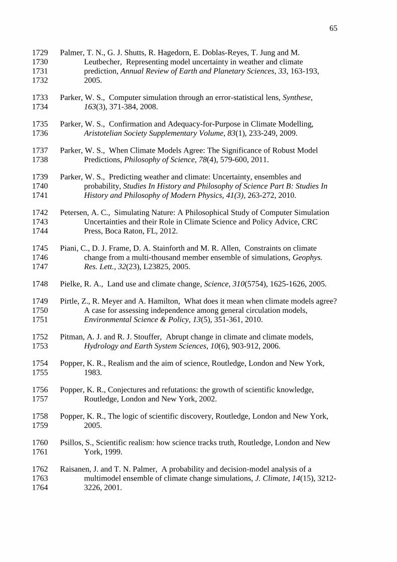
65
Palmer, T. N., G. J. Shutts, R. Hagedorn, E. Doblas-Reyes, T. Jung and M. 1729
Leutbecher, Representing model uncertainty in weather and climate 1730
prediction, Annual Review of Earth and Planetary Sciences, 33, 163-193, 1731
2005. 1732
Parker, W. S., Computer simulation through an error-statistical lens, Synthese, 1733
163(3), 371-384, 2008. 1734
Parker, W. S., Confirmation and Adequacy-for-Purpose in Climate Modelling, 1735
Aristotelian Society Supplementary Volume, 83(1), 233-249, 2009. 1736
Parker, W. S., When Climate Models Agree: The Significance of Robust Model 1737
Predictions, Philosophy of Science, 78(4), 579-600, 2011. 1738
Parker, W. S., Predicting weather and climate: Uncertainty, ensembles and 1739
probability, Studies In History and Philosophy of Science Part B: Studies In 1740
History and Philosophy of Modern Physics, 41(3), 263-272, 2010. 1741
Petersen, A. C., Simulating Nature: A Philosophical Study of Computer Simulation 1742
Uncertainties and their Role in Climate Science and Policy Advice, CRC 1743
Press, Boca Raton, FL, 2012. 1744
Piani, C., D. J. Frame, D. A. Stainforth and M. R. Allen, Constraints on climate 1745
change from a multi-thousand member ensemble of simulations, Geophys. 1746
Res. Lett., 32(23), L23825, 2005. 1747
Pielke, R. A., Land use and climate change, Science, 310(5754), 1625-1626, 2005. 1748
Pirtle, Z., R. Meyer and A. Hamilton, What does it mean when climate models agree? 1749
A case for assessing independence among general circulation models, 1750
Environmental Science & Policy, 13(5), 351-361, 2010. 1751
Pitman, A. J. and R. J. Stouffer, Abrupt change in climate and climate models, 1752
Hydrology and Earth System Sciences, 10(6), 903-912, 2006. 1753
Popper, K. R., Realism and the aim of science, Routledge, London and New York, 1754
1983. 1755
Popper, K. R., Conjectures and refutations: the growth of scientific knowledge, 1756
Routledge, London and New York, 2002. 1757
Popper, K. R., The logic of scientific discovery, Routledge, London and New York, 1758
2005. 1759
Psillos, S., Scientific realism: how science tracks truth, Routledge, London and New 1760
York, 1999. 1761
Raisanen, J. and T. N. Palmer, A probability and decision-model analysis of a 1762
multimodel ensemble of climate change simulations, J. Climate, 14(15), 3212-1763
3226, 2001. 1764
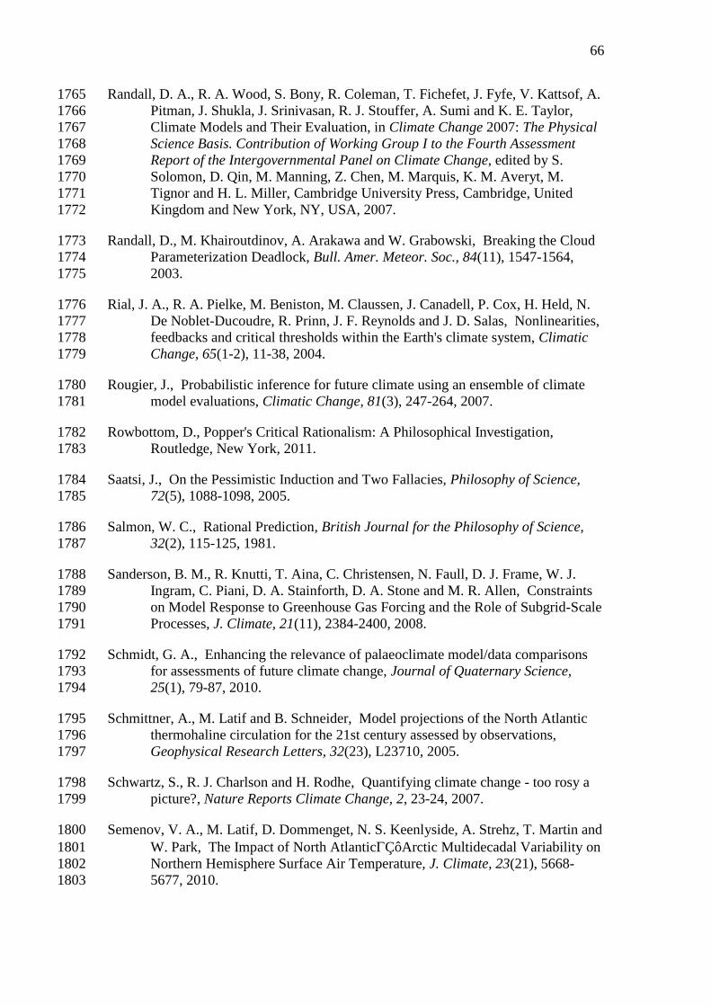
66
Randall, D. A., R. A. Wood, S. Bony, R. Coleman, T. Fichefet, J. Fyfe, V. Kattsof, A. 1765
Pitman, J. Shukla, J. Srinivasan, R. J. Stouffer, A. Sumi and K. E. Taylor, 1766
Climate Models and Their Evaluation, in Climate Change 2007: The Physical 1767
Science Basis. Contribution of Working Group I to the Fourth Assessment 1768
Report of the Intergovernmental Panel on Climate Change, edited by S. 1769
Solomon, D. Qin, M. Manning, Z. Chen, M. Marquis, K. M. Averyt, M. 1770
Tignor and H. L. Miller, Cambridge University Press, Cambridge, United 1771
Kingdom and New York, NY, USA, 2007. 1772
Randall, D., M. Khairoutdinov, A. Arakawa and W. Grabowski, Breaking the Cloud 1773
Parameterization Deadlock, Bull. Amer. Meteor. Soc., 84(11), 1547-1564, 1774
2003. 1775
Rial, J. A., R. A. Pielke, M. Beniston, M. Claussen, J. Canadell, P. Cox, H. Held, N. 1776
De Noblet-Ducoudre, R. Prinn, J. F. Reynolds and J. D. Salas, Nonlinearities, 1777
feedbacks and critical thresholds within the Earth's climate system, Climatic 1778
Change, 65(1-2), 11-38, 2004. 1779
Rougier, J., Probabilistic inference for future climate using an ensemble of climate 1780
model evaluations, Climatic Change, 81(3), 247-264, 2007. 1781
Rowbottom, D., Popper's Critical Rationalism: A Philosophical Investigation, 1782
Routledge, New York, 2011. 1783
Saatsi, J., On the Pessimistic Induction and Two Fallacies, Philosophy of Science, 1784
72(5), 1088-1098, 2005. 1785
Salmon, W. C., Rational Prediction, British Journal for the Philosophy of Science, 1786
32(2), 115-125, 1981. 1787
Sanderson, B. M., R. Knutti, T. Aina, C. Christensen, N. Faull, D. J. Frame, W. J. 1788
Ingram, C. Piani, D. A. Stainforth, D. A. Stone and M. R. Allen, Constraints 1789
on Model Response to Greenhouse Gas Forcing and the Role of Subgrid-Scale 1790
Processes, J. Climate, 21(11), 2384-2400, 2008. 1791
Schmidt, G. A., Enhancing the relevance of palaeoclimate model/data comparisons 1792
for assessments of future climate change, Journal of Quaternary Science, 1793
25(1), 79-87, 2010. 1794
Schmittner, A., M. Latif and B. Schneider, Model projections of the North Atlantic 1795
thermohaline circulation for the 21st century assessed by observations, 1796
Geophysical Research Letters, 32(23), L23710, 2005. 1797
Schwartz, S., R. J. Charlson and H. Rodhe, Quantifying climate change - too rosy a 1798
picture?, Nature Reports Climate Change, 2, 23-24, 2007. 1799
Semenov, V. A., M. Latif, D. Dommenget, N. S. Keenlyside, A. Strehz, T. Martin and 1800
W. Park, The Impact of North AtlanticÇôArctic Multidecadal Variability on 1801
Northern Hemisphere Surface Air Temperature, J. Climate, 23(21), 5668-1802
5677, 2010. 1803
67
Shackley, S., Epistemic lifestyles in climate change modeling, in Changing the 1804
atmosphere, edited by C. A. Miller and Edwards P.N., pp. 109-133, The MIT 1805
Press, Cambridge Mass. and London, 1997. 1806
Shukla, J., T. DelSole, M. Fennessy, J. Kinter and D. Paolino, Climate model fidelity 1807
and projections of climate change, Geophys. Res. Lett., 33(7), L07702, 2006. 1808
Siddall, M., A. be-Ouchi, M. Andersen, F. Antonioli, J. Bamber, E. Bard, J. Clark, P. 1809
Clark, P. Deschamps, A. Dutton, M. Elliot, C. Gallup, N. Gomez, J. Gregory, 1810
P. Huybers, K. Kawarnura, M. Kelly, K. Lambeck, T. Lowell, J. Milrovica, B. 1811
Otto-Bliesner, D. Richards, J. Stanford, C. Stirling, T. Stocker, A. Thomas, B. 1812
Thompson, T. Tornqvist, N. V. Riveiros, C. Waelbroeck, Y. Yokoyama and S. 1813
Y. Yu, The sea-level conundrum: case studies from palaeo-archives, Journal 1814
of Quaternary Science, 25(1), 19-25, 2010. 1815
Smith, L. A., Predictability past, predictability present, in Predictability of Weather 1816
and Climate, edited by T. Palmer and R. Hagedorn, pp. 217-250, Cambridge 1817
University Press, Cambridge, 2006. 1818
Snyder, C. W., The value of paleoclimate research in our changing climate, Climatic 1819
Change, 100(3-4), 407-418, 2010. 1820
Sober, E., Bayesianism — its Scope and Limits, in Bayes' Theorem, edited by R. 1821
Swinburne, pp. 21-38, Oxford University Press, Oxford, 2002. 1822
Spicer, R. A., A. Ahlberg, A. B. Herman, C. C. Hofmann, M. Raikevich, P. J. Valdes 1823
and P. J. Markwick, The Late Cretaceous continental interior of Siberia: A 1824
challenge for climate models, Earth and Planetary Science Letters, 267(1-2), 1825
228-235, 2008. 1826
Stainforth, D. A., T. Aina, C. Christensen, M. Collins, N. Faull, D. J. Frame, J. A. 1827
Kettleborough, S. Knight, A. Martin, J. M. Murphy, C. Piani, D. Sexton, L. A. 1828
Smith, R. A. Spicer, A. J. Thorpe and M. R. Allen, Uncertainty in predictions 1829
of the climate response to rising levels of greenhouse gases, Nature, 1830
433(7024), 403-406, 2005. 1831
Stainforth, D. A., M. R. Allen, E. R. Tredger and L. A. Smith, Confidence, 1832
uncertainty and decision-support relevance in climate predictions, 1833
Philosophical Transactions of the Royal Society A-Mathematical Physical and 1834
Engineering Sciences, 365(1857), 2145-2161, 2007a. 1835
Stainforth, D. A., T. E. Downing, R. Washington, A. Lopez and M. New, Issues in 1836
the interpretation of climate model ensembles to inform decisions, 1837
Philosophical Transactions of the Royal Society A-Mathematical Physical and 1838
Engineering Sciences, 365(1857), 2163-2177, 2007b. 1839
Stanford, P. K., Exceeding Our Grasp: Science, History, and the Problem of 1840
Unconceived Alternatives, Oxford University Press, New York, 2006. 1841
Stott, P. A., J. F. B. Mitchell, M. R. Allen, T. L. Delworth, J. M. Gregory, G. A. 1842
Meehl and B. D. Santer, Observational Constraints on Past Attributable 1843

68
Warming and Predictions of Future Global Warming, J. Climate, 19(13), 1844
3055-3069, 2006. 1845
Strevens, M., Probability and chance, in Macmillan Encyclopedia of Philosophy, vol. 1846
8, edited by D. M. Borchert, pp. 24-40, MacMillan Reference USA. Thomson 1847
Gale., New York, 2006a. 1848
Strevens, M., The Bayesian Approach to the Philosophy of Science, in Encyclopedia 1849
of Philosophy, edited by D. M. Borchert, Macmillan Reference, Detroit, 1850
2006b. 1851
Swanson, K. L., G. Sugihara and A. A. Tsonis, Long-term natural variability and 1852
20th century climate change, Proceedings of the National Academy of 1853
Sciences, 106(38), 16120-16123, 2009. 1854
Tebaldi, C. and R. Knutti, The use of the multi-model ensemble in probabilistic 1855
climate projections, Philosophical Transactions of the Royal Society A-1856
Mathematical Physical and Engineering Sciences, 365(1857), 2053-2075, 1857
2007. 1858
Tebaldi, C., R. L. Smith, D. Nychka and L. O. Mearns, Quantifying uncertainty in 1859
projections of regional climate change: A Bayesian approach to the analysis of 1860
multimodel ensembles, J. Climate, 18(10), 1524-1540, 2005. 1861
Thagard, P. R., Best Explanation - Criteria for Theory Choice, Journal of Philosophy, 1862
75(2), 76-92, 1978. 1863
Valdes, P., Built for stability, Nature Geosci, 4(7), 414-416, 2011. 1864
Vineberg, S., Dutch Book Arguments (on line), the Stanford Encyclopedia of 1865
Philosophy, http://plato. stanford. edu/archives/sum2011/entries/dutch-book/, 1866
2011. 1867
Weisberg, M., Robustness analysis, Philosophy of Science, 73(5), 730-742, 2006. 1868
Wigley, T. M. L., Climate-Change - Outlook Becoming Hazier, Nature, 369(6483), 1869
709-710, 1994. 1870
Winsberg, E., Models of success versus the success of models: Reliability without 1871
truth, Synthese, 152(1), 1-19, 2006. 1872
Worrall, J., Error, tests and theory confirmation, in Error and Inference: Recent 1873
Exchanges on Experimental Reasoning, Reliability, and the Objectivity and 1874
Rationality of Science, edited by D. G. Mayo and A. Spanos, pp. 125-154, 1875
Cambridge University Press, New York, 2010. 1876
Wu, Z., N. Huang, J. Wallace, B. Smoliak and X. Chen, On the time-varying trend in 1877
global-mean surface temperature, Climate Dynamics, 1-15, 2011. 1878
Wunsch, C., Towards understanding the Paleocean, Quaternary Science Reviews, 1879
29(17-18), 1960-1967, 2010. 1880

69
Wyatt, M., S. Kravtsov and A. Tsonis, Atlantic Multidecadal Oscillation and 1881
Northern Hemisphere's climate variability, Climate Dynamics, 1-21, 2011. 1882
1883
Captions 1884
Fig. 1 Temperature changes relative to the corresponding average for 1901-1950 1885
(°C) from decade to decade from 1906 to 2005 over the entire globe, global land area 1886
and the global ocean. The black line indicates observed temperature change, while 1887
the colored bands show the combined range covered by 90% of recent model 1888
simulations. Red indicates simulations that include natural and human factors, while 1889
blue indicates simulations that include only natural factors. Dashed black lines 1890
indicate decades and continental regions for which there are substantially fewer 1891
observations. Adapted from Hegerl et al., FAQ9.2, Fig. 1 (2007, p. 703). 1892
1893
Fig. 2 Projected 21st century global mean temperatures changes for various 1894
greenhouse gas emission scenarios. Solid lines are multi-model global averages of 1895
surface warming for scenarios A2, A1B and B1, shown as continuations of the 20th-1896
century simulations. These projections also take into account emissions of short-lived 1897
GHGs and aerosols. The pink line is not a scenario, but is for Atmosphere-Ocean 1898
General Circulation Model (AOGCM) simulations where atmospheric concentrations 1899
are held constant at year 2000 values. The bars at the right of the figure indicate the 1900
best estimate (solid line within each bar) and the likely range assessed for the six 1901
SRES marker scenarios at 2090-2099. All temperatures are relative to the period 1902
1980-1999. Adapted from the Synthesis Report for IPCC AR4, Fig. 3.2 (2007, p. 7). 1903
1904
Fig. 3 Evolution of the MOC at 30°N in simulations with the suite of comprehensive 1905
coupled climate models from 1850 to 2100 using 20th Century Climate in Coupled 1906
Models (20C3M) simulations for 1850 to 1999 and the SRES A1B emissions scenario 1907
for 1999 to 2100. Some of the models continue the integration to year 2200 with the 1908
forcing held constant at the values of year 2100. Observationally based estimates of 1909
late-20th century MOC are shown as vertical bars on the left. Adapted from Meehl et 1910
al., Fig. 10.15 (2007b, p. 773), who build on Schmittner et al. (2005). 1911
1912
Fig. 4. Root-mean-square (RMS) error of 1980–99 surface temperature (averaged 1913
over space, relative to the 40-year reanalysis of the European Centre of Medium 1914
range Weather Forecast) shown as a function of the number of models included in the 1915
model average. Panel (a) shows the December-January-February period (DJF), 1916
panel (b) the June-July-August (JJA) period. Red dashed lines indicate the range 1917
covered by randomly sampling the models for the subset; the red solid line indicates 1918
the average. The RMS error converges to a constant value that is more than half of 1919
the initial value for one model. The black dashed line is a theoretical RMS. If the 1920
model biases were independent, then the RMS error for a large sample of models 1921
should decrease with the square root of the number of models (dotted). The blue line 1922
results if the models are sorted by how well they agree with DJF and JJA 1923
observations combined, and it indicates that the average of a few good models 1924
outperforms an average of more models with poorer performance. Adapted from 1925
Knutti et al., Figs 3(c) and 3(d) (2010, p. 2744). 1926
1927
Fig. 5 Constraints on the radiative forcing from the observed atmospheric and 1928
oceanic warming. Probability density functions (PDF) for the total (anthropogenic 1929
and natural) radiative forcing (a–c) and the indirect aerosol forcing (d–f) in the year 1930
70
2000 are based on 25,000 Monte Carlo simulations. The initially assumed PDFs are 1931
given in a and d. The requirement that the model matches the temperature 1932
observations strongly narrows the PDFs (b and e). If in addition the climate 1933
sensitivity is restricted to the range adopted by the IPCC (1.5–4.5 K), the PDFs in c 1934
and f are obtained. Adapted from Knutti et al., Fig. 2 (2002, p. 720). 1935
1936
Fig. 6. The response to parameter perturbations: the frequency distribution of 1937
simulated climate sensitivity using all model versions (black), all model versions 1938
except those with perturbations to the cloud-to-rain conversion threshold (red), and 1939
all model versions except those with perturbations to the entrainment coefficient 1940
(blue). Adapted from Stainforth et al, Fig. 2(a) (2005, p. 404). 1941
1942
Figures 1943
1944 Fig. 1 1945
1946
1947
Fig. 2 1948
1949
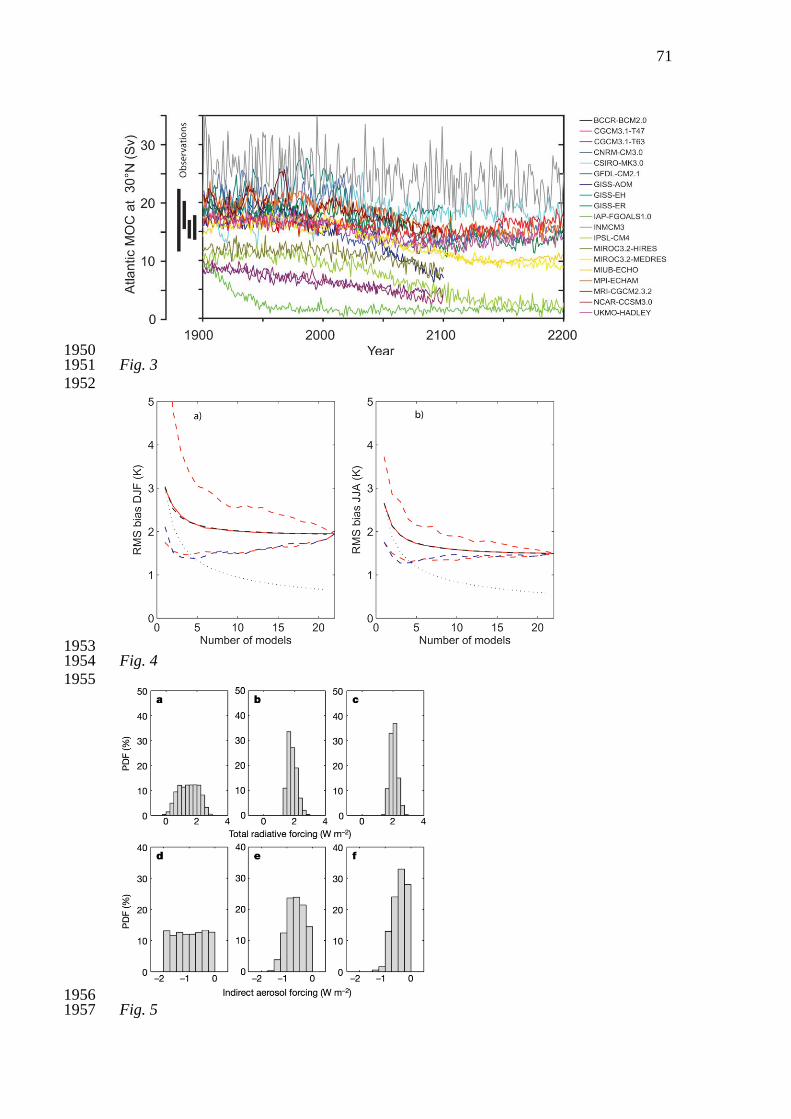
71
1950 Fig. 3 1951
1952
1953 Fig. 4 1954
1955
1956 Fig. 5 1957
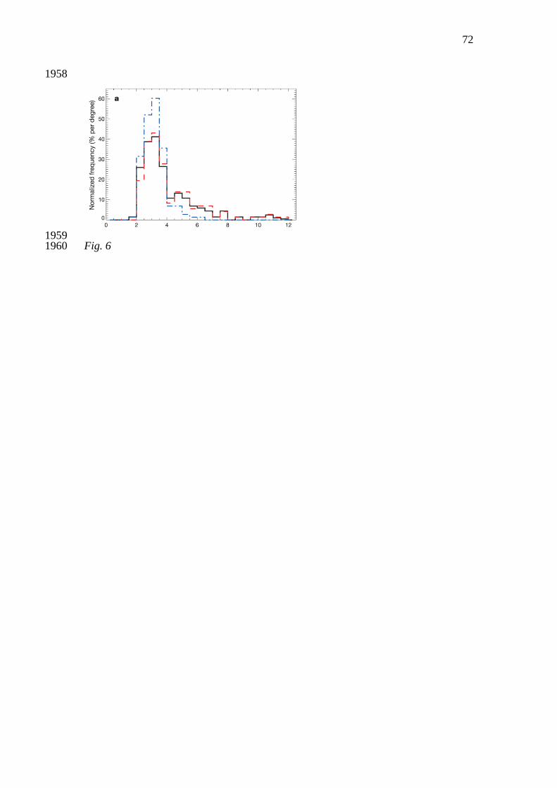
72
1958
1959 Fig. 6 1960