2015 report - santa barbara - home
TRANSCRIPT

SOUTHERN COASTAL
SANTA BARBARA STREAMS AND ESTUARIES
BIOASSESSMENT PROGRAM
2015 REPORT
Prepared for:
City of Santa Barbara, Creeks Division
County of Santa Barbara,
Project Clean Water
Prepared By:
www.ecologyconsultantsinc.com

Ecology Consultants, Inc.
Southern Coastal Santa Barbara Streams and Estuaries Bioassessment Program Page 2 2015 Report
Executive Summary Introduction
This report summarizes the results of the 2015 Southern Coastal Santa Barbara Streams and Estuaries Bioassessment Program, an effort funded by the City of Santa Barbara and County of Santa Barbara. This is the 16th year of the Program, which began in 2000. Ecology Consultants, Inc. (Ecology) prepared this report, and serves as the City and County’s consultant for the Program. The purpose of the Program is to assess and monitor the “biological integrity” of study streams and estuaries as they respond through time to natural and human influences. The Program involves annual collection and analyses of benthic macroinvertebrate (BMI) samples and other pertinent physiochemical and biological data at study streams and estuaries using U.S. Environmental Protection Agency (USEPA) endorsed rapid bioassessment methodology. BMI samples are analyzed in the laboratory to determine BMI abundance, composition, and diversity. Study sites have included the range available along a disturbance gradient, from “reference” sites that are fairly intact in form with little urbanization in their watersheds to “highly disturbed” sites that have been substantially altered in form and drain highly urbanized watersheds. Intermediate “moderately disturbed” sites have also been surveyed.
Local streams have been studied since 2000, and a BMI based Index of Biological Integrity (IBI) was constructed by Ecology in 2004, and updated in 2009 and again last year. The IBI yields a numeric score and classifies the biological integrity of a given stream as Very Poor, Poor, Fair, Good, or Excellent based on the contents of the BMI sample collected from the stream. By condensing complex biological data into an easily understood score and classification of biological integrity, the IBI serves as an effective tool for the City and County in monitoring the condition of local streams, and evaluating the benefits or consequences of watershed management actions. Local estuaries have been studied since 2011. A major goal is to identify several reliable BMI indicator metrics that show significant differences trends along a disturbance gradient in local estuaries. Such indicator BMI metrics will be the foundation in developing a reliable IBI or similar tool for assessing the condition of local estuaries, which hopefully can be produced after another year or two of study.
Study Area
The study area encompasses approximately 80 km of the southern Santa Barbara County coast from the Rincon Creek watershed at the Santa Barbara/Ventura County line west to Jalama Creek just north of Point Conception. There are approximately 50 1st to 5th order coastal streams along this stretch of coast, all of which drain the southern face of the Santa Ynez Mountains. 51 different stream study reaches in 20 watersheds have been surveyed on one or more occasions during the 16 years of the Program, while 10 different estuaries have been studied once or more over the last 5 years.
Results
Over the past 16 years, the Program has provided a wealth of information regarding the physiochemical habitat conditions and biota (particularly the BMI community) of local streams, and the influences of natural physiochemical and climatic variability and human development. The following statements can be made based on the research completed thus far:

Ecology Consultants, Inc.
Southern Coastal Santa Barbara Streams and Estuaries Bioassessment Program Page 3 2015 Report
• Negative impacts of human land use on local stream communities (particularly BMIs) have been documented with highly significant statistical test results. Degradation of stream communities (e.g., lower IBI scores and loss of sensitive species), as well as physiochemical habitat conditions, has increased linearly with increased watershed development. Urban development has been shown to have greater impacts on stream communities than has agricultural development.
• The IBI is highly effective as an indicator of biological integrity, with highly significant relationships with indicies of human disturbance. The IBI has properly differentiated between REF, MOD DIST, and HIGH DIST with a high degree of accuracy and consistency.
• Major episodic disturbances including extreme stream flows, drought conditions, and wildfires have been definitively shown to negatively impact stream communities, as evidenced by lower IBI scores and loss or significant reduction of sensitive BMI and vertebrate taxa following such events. In recent years, BMI communities have progressively declined at several sites in response to prolonged drought and resulting loss of flow and low dissolved oxygen levels. Local stream BMI communities have proven to be resilient, typically showing dramatic recovery from extreme episodic disturbances in a year or two. However, some of the more sensitive species (e.g., rainbow trout) have yet to return to streams impacted by wildfires, drought, and/or floods, and may require many years to recover.
• Stream habitat restoration sites M2 and AB5 have shown improved habitat conditions, but significant improvements in the BMI community have not occurred thus far. Channel and riparian restoration at these sites did not address larger scale impairments in hydrology, geomorphology, water quality, habitat continuity and connectivity that have resulted from alteration of their respective watersheds. Whether or not current and future restoration efforts will improve the BMI community at M2 and AB5 can only be evaluated via continued monitoring through time.
The Program effort to study local estuaries is still new relative to our study of streams. Based on the limited data set available for estuaries, the following can be stated thus far:
• Determining the impacts of human land use on the BMI communities in local estuaries has proven to be more difficult compared with streams. One reason for this is the fact that there are fewer estuaries in the study area compared with streams, particularly in the REF category (i.e., only Gaviota and Jalama studied thus far). Also, wide salinity fluctuations make estuaries harsh environments where a relatively small number of BMI taxa can survive when compared with streams. Taxa richness has not proven to be a reliable indicator of estuary condition as it has in streams. We have identified several taxa that are more abundant in the REF estuaries, which are the basis of the metric % sens BMIs. This and possibly other metrics may be utilized to develop and IBI or similar assessment tool for local estuaries.
• More replication and diversification of REF estuaries having greater physiochemical variability will be needed to gain more confidence in our ability to understand the influences of salinity and other physiochemical parameters on indicator BMI metrics.

Ecology Consultants, Inc.
Southern Coastal Santa Barbara Streams and Estuaries Bioassessment Program Page 4 2015 Report
TABLE OF CONTENTS
Page I. INTRODUCTION .......................................................................................................... 6 II. STUDY AREA ............................................................................................................ 12 III. METHODS ............................................................................................................ 17
A. Field Surveys ............................................................................................. 17 B. Laboratory Analysis .................................................................................... 19 C. GIS Analyses ............................................................................................. 20 D. Review of Topographic Maps and Aerial Photographs ................................... 20 E. Study Reach Grouping ................................................................................ 20 F. Calculation of Core Metrics for Streams ....................................................... 21 G. Core Metric Scoring Ranges for Streams ...................................................... 22 H. IBI Classifications of Biological Integrity and Scoring Ranges for Streams ...... 22 I. Data Analyses for Streams .......................................................................... 23 J. Calculation of BMI Metrics for Estuaries ....................................................... 24 K. Evaluating Estuary BMI Taxa and Metrics for Disturbance Sensitivity ............. 25 L. Evaluating Salinity Effects on Estuary BMI Taxa and Metrics ......................... 25
IV. RESULTS AND DISCUSSION .......................................................................................... 26 A. Physiochemical and Biological Data ............................................................. 26 B. Streams .................................................................................................... 26 C. Estuaries ................................................................................................... 47
V. CLOSING ............................................................................................................ 61 VI. ACKNOWLEDGEMENTS ................................................................................................ 63 VI. REFERENCES ............................................................................................................ 64 APPENDIX: DATA TABLES AND ESTUARY HABITAT ASSESSMENT SCORING SHEET
PLATES Page
Plate 1 Reference Stream Reach Example ................................................................. 9 Plate 2 Disturbed Stream Reach Example ............................................................... 10
FIGURES Page
Figure 1 Study Area ................................................................................................ 13 Figure 2 Gaviota Coast Study Reaches...................................................................... 14 Figure 3 Santa Barbara and Goleta Area Study Reaches ........................................... 15 Figure 4 Carpinteria Area Study Reaches .................................................................. 16 Figure 5 Carpinteria Creek Watershed IBI Scores ...................................................... 28 Figure 6 Sycamore Creek Watershed IBI Scores ........................................................ 30 Figure 7 Mission Creek Watershed IBI Scores ........................................................... 34 Figure 8 Arroyo Burro Creek Watershed IBI Scores ................................................... 36 Figure 9 San Jose Creek Watershed IBI Scores ......................................................... 38

Ecology Consultants, Inc.
Southern Coastal Santa Barbara Streams and Estuaries Bioassessment Program Page 5 2015 Report
Figure 10 Arroyo Hondo Creek Watershed IBI Scores .................................................. 40 Figure 11 Gaviota Creek Watershed IBI Scores ........................................................... 41 Figure 12 ANOVAs of IBI Score for F-F, F-P, and P-P Flow Groups ............................... 43 Figure 13 ANOVAs of IBI Score for REF Reaches by Year ............................................ 44 Figure 14 ANOVAs of IBI Score for HIGH DIST, MOD DIST, and REF Groups for Selected Years ........................................................................................... 46 Figure 15 ANOVAs of Mean Abundance of Selected BMI Taxa in Estuaries .................... 57 Figure 16 ANOVAs of % Sensitive BMIs and % Tolerant BMIs in Estuaries ................... 58 Figure 17 Linear Regression of % Sensitive BMIs vs. Salinity, REF Group ..................... 59
TABLES Page
Table 1 Study Reaches ........................................................................................... 12 Table 2 Core Metric Scoring Ranges ........................................................................ 22 Table 3 IBI Classifications of Biological Integrity ...................................................... 23 Table 4 BMI Metrics Calculated for Study Estuaries .................................................. 24

Ecology Consultants, Inc.
Southern Coastal Santa Barbara Streams and Estuaries Bioassessment Program Page 6 2015 Report
I. Introduction
This report summarizes the results of the 2015 Southern Coastal Santa Barbara Streams and Estuaries Bioassessment Program, an effort funded by the City of Santa Barbara and County of Santa Barbara. This is the 16th year of the Program, which began in 2000. Ecology Consultants, Inc. (Ecology) prepared this report, and serves as the City and County’s consultant for the Program. The purpose of the Program is to assess and monitor the “biological integrity” of study streams and estuaries as they respond through time to natural and human influences. The Program involves annual collection and analyses of benthic macroinvertebrates (BMIs) and other pertinent physiochemical and biological data at study streams and estuaries using United States Environmental Protection Agency (USEPA) endorsed rapid bioassessment methodology. BMIs are aquatic insects, crustaceans, mollusks, worms, and other invertebrates of a half-millimeter in length or greater that inhabit the bottom substrata of streams, lakes, ponds, estuaries, ocean waters, and other water bodies for at least part of their life cycles. BMI samples are analyzed in the laboratory to determine BMI abundance, composition, and diversity. Scores and classifications of biological integrity are determined for study streams using the BMI based Index of Biological Integrity (IBI) constructed by Ecology. The IBI was initially built in 2004, updated in 2009, and updated again last year in 2014.
What is biological integrity?
“Biological integrity” can be defined as “the ability (of a water body) to support and maintain a balanced, integrated, adaptive community of organisms having a species composition, diversity, and functional organization comparable to that of natural habitat of the region.” (Miller et al., 1988). In other words, biological integrity can be thought of as the overall biological condition of a water body in comparison to natural, more or less pristine habitat in the same region. Natural perturbations such as heavy floods, droughts, and wildfires, as well as human disturbances (e.g., to hydrology, geomorphology, water chemistry, etc.) have been shown to negatively impact the biological integrity of waters locally and around the world.
How do we determine, or measure, biological integrity?
“Bioassessment” is the science of determining, or measuring, the biological integrity of water bodies by evaluating the composition of the biological communities that inhabit them. The origins of bioassessment in the United States and Europe date back to the late 1800’s. Within the last 30 years, the incorporation of bioassessment into water monitoring programs has increased dramatically throughout the United States because of the development of rapid, cost-effective assessment and data analysis techniques (Rosenberg and Resh, 1993). Currently, bioassessment is used throughout the U.S. and the world to assess, monitor, and manage the integrity of streams, rivers, lakes, ponds, estuaries, and coastal marine waters.
The foundation of bioassessment is the fact that individual aquatic species have varying habitat requirements and abilities to withstand natural and human disturbances. Thus, the composition of the biological community, or the species present and their relative abundances, provides a valuable indication of biological integrity. The disturbance sensitivity of each unique species depends on their physiology, size, habitat requirements, survival strategy (i.e., primary producer, filter feeder, grazer, predator, etc.), and of course the nature of the disturbance(s).

Ecology Consultants, Inc.
Southern Coastal Santa Barbara Streams and Estuaries Bioassessment Program Page 7 2015 Report
As an example, the presence of viable salmonid populations in coastal California streams generally indicates good biological integrity. To thrive, salmonids require cool, clean, well-oxygenated stream water, clean cobble/gravel beds for spawning, deep pools for cover from predators, and an adequate aquatic invertebrate and vertebrate prey base. Salmonids are especially sensitive to increased fine sediment loads, higher stream temperatures, low dissolved oxygen levels, water pollutants, and other habitat modifications such as the construction of dams and other migration barriers that typically occur in areas with intensive human development. While species such as salmonids that are sensitive to habitat disturbances are typically reduced or eliminated in highly disturbed water bodies, disturbance tolerant species may persist or even flourish. Disturbed waters typically have a biological community composed of a smaller number of more disturbance tolerant taxa compared to more natural, pristine waters, which typically have higher numbers of taxa, including those that are disturbance sensitive.
Beyond individual species, measurements of the biological community, or “biological metrics”, relating to abundance, species richness, proportion of disturbance sensitive species, and trophic structure have been shown to be reliable indicators of biological integrity in hundreds of bioassessment studies around the world. The reliability of such metrics as indicators of biological integrity depends on the strength of their relationships with measures of habitat disturbance.
How does human development impact habitat conditions in local streams and estuaries?
The study area encompasses the southern slopes of the Santa Ynez mountains from the Santa Barbara/Ventura County line to Point Conception. In general, human development is minimal in the northern mountainous areas, with some grazing, orchards and light residential uses in the foothills, transitioning to more intensive agriculture and urban development further southward where there are extensive coastal plains. The majority of development is concentrated in the cities of Santa Barbara, Goleta, and Carpinteria. Disturbance is limited mostly to orchards, grazing, and rural residential uses west of Goleta to Point Conception.
Generally, the nature and magnitude of disturbance in local streams and estuaries is proportional to the cumulative intensity and extent of development in their watersheds. Plates
Rainbow trout in Rattlesnake Creek
View to south from East Camino Cielo above Rattlesnake Canyon (Mission Creek drainage)

Ecology Consultants, Inc.
Southern Coastal Santa Barbara Streams and Estuaries Bioassessment Program Page 8 2015 Report
1 and 2 provide examples of two stream study reaches: (1) a relatively pristine stream in the undeveloped mountains, and (2) a disturbed stream on the urbanized coastal plain. The plates show the positions of these two stream reaches in their respective watersheds, surrounding land uses, and photographs of stream habitat conditions and aquatic species. Common forms of human disturbance in local streams and estuaries include: (1) altered hydrology and geomorphology due to water diversions, urban and agricultural land development, and flood control projects; (2) burying of stream and estuary substrate due to increased deposition of fine sediments from eroding agricultural fields and stream banks; (3) loss of riparian and upland habitat essential to many aquatic species; (4) loss of stream and estuary habitat complexity, algal blooms, elevated water temperatures, wider fluctuations in dissolved oxygen, and loss of energy inputs due stream channelization and removal of riparian vegetation; (5) degraded water quality due to inputs of fertilizers, pesticides, petroleum hydrocarbons, heavy metals, and other pollutants; (6) habitat fragmentation and barriers to species movement and migration due to the construction of in-stream barriers such as dams, road crossings, bridges, and culverts; (7) introductions of invasive, non-native plants and animals, which can outcompete and threaten the long-term viability of native species; and (8) disturbances to vegetation and/or wildlife associated with trampling, noise, lighting, air pollution, and predation by domestic pets.
What is the streams IBI? What does it tell us?
The streams IBI developed for this Program is a multimetric tool that provides a standardized, integrative, and readily understandable scale for measuring the biological integrity of local streams. Because biological assemblages vary in response to natural physical and chemical gradients that occur through geographic space, IBIs are calculated for specific regions and water body types (i.e., streams, lakes, estuaries, etc.) with similar ecological characteristics. The term multimetric refers to an IBI being constructed by combining several individual biological metrics into a single index. Our IBI uses 7 BMI metrics derived from the BMI samples collected at the study stream reaches. These “core metrics” are all highly sensitive to human disturbance as determined through rigorous statistical analyses, and collectively represent several aspects of BMI community structure including relative abundances of disturbance sensitive and tolerant taxa, taxonomic richness, and trophic structure. Values for each core metric at a study stream are scored on a dimensionless numeric scale (e.g., from 0 to 10) relative to the known distribution of values for sites along a human disturbance gradient. Higher scores (e.g., a 10) represent the conditions at the most pristine sites, whereas lower scores indicate greater departure from pristine conditions. Scores assigned to the individual core metrics are equally weighted and combined into an overall score. The IBI classifies the biological integrity of a given stream as Very Poor, Poor, Fair, Good, or Excellent based on the overall score. The IBI serves as an effective tool for the City and County in monitoring the condition of local streams, devising and prioritizing watershed management actions, and evaluating their benefits or consequences.
BMI sampling in Gobernador Creek

Ecology Consultants, Inc.
Southern Coastal Santa Barbara Streams and Estuaries Bioassessment Program Page 9 2015 Report
Plate 1: Reference Stream Reach Example
Stream reach location marked on map (left) by black dot. Upstream watershed drains wilderness lands (olive green and brown in map). Downstream agricultural (light green) and urban (grey) lands (downstream) do not affect this stream reach. Stream has unaltered hydrology and form, with natural bed and banks, alternating riffles and pools, boulder and cobble beds (no excessive fine sediments), and intact mostly native riparian vegetation with mature canopy trees. Stream habitat is optimal for a variety of aquatic and riparian species, including a diverse BMI community and several sensitive aquatic vertebrates including rainbow/steelhead trout, California newt, and southwestern pond turtle (below).

Ecology Consultants, Inc.
Southern Coastal Santa Barbara Streams and Estuaries Bioassessment Program Page 10 2015 Report
Plate 2: Disturbed Stream Reach Example
Stream reach location marked on map (left) by black dot. Stream drains urban (grey), agricultural (light green) and wilderness lands (olive green/brown). Impervious surfaces (urban), channelization, and increased fine sediment loads (agriculture) have altered stream hydrology and form, and water pollutants (e.g., nutrients, pesticides, hydrocarbons) are present. Stream banks have been largely denuded of native vegetation, resulting in unstable, eroding banks, establishment of invasive non-native plants (e.g., Arundo donax below), algal blooms, and wide fluctuations in water temperature and dissolved oxygen. Fine sediments largely smother boulder, cobble, and gravel that would provide stable aquatic habitat. Sensitive BMIs and aquatic vertebrates are largely absent due to habitat degradation.

Ecology Consultants, Inc.
Southern Coastal Santa Barbara Streams and Estuaries Bioassessment Program Page 11 2015 Report
Why use BMIs? There are several reasons why BMIs are useful as biological indicators. First, BMIs are a critical component of aquatic ecosystems, often representing a large proportion of community biomass, performing important functions in the cycling of nutrients and energy, and constituting food sources for vertebrate predators such as fish and amphibians. Major changes in BMI assemblages can have profound ramifications for aquatic ecosystems. Secondly, the responsiveness of BMIs to environmental perturbations, including human impacts, is well documented. Information is available on the life histories, distributions, habitat requirements, and disturbance tolerances of most BMIs. In the case of local streams, BMIs also are far more abundant and diverse compared to aquatic vertebrates (e.g., fish and amphibians), and are relatively easy to collect.
Estuaries
In 2011 the Program was expanded to include estuaries. Estuaries are open water bodies where a freshwater stream meets and mixes with saltwater from the ocean, creating brackish water conditions with salinities that vary depending on fluctuating seasonal inputs from the stream and ocean. USEPA endorsed rapid bioassessment methods for estuaries have been used to collect BMI samples and other pertinent physiochemical and biological data in local estuaries.
Over the past 5 years a data set has been compiled for local estuaries. Study sites have included the range available along a disturbance gradient, from “reference” sites that are fairly intact in form with little urbanization in their watersheds to “highly disturbed” sites that have been substantially altered in form and drain highly urbanized watersheds. Intermediate “moderately disturbed” sites have also been surveyed. A total of 9 estuaries were studied this year. A goal in studying local estuaries is to identify reliable BMI indicator metrics that show significant trends along a disturbance gradient. Hopefully, such indicator BMI metrics will be the foundation in developing an IBI or similar tool for local estuaries within the next year or two.
Stoneflies and Hemiptera in Gobernador Creek
Mission Creek estuary (high disturbance)
Jalama Creek estuary (low disturbance)
Ecology Consultants, Inc.
Southern Coastal Santa Barbara Streams and Estuaries Bioassessment Program Page 12 2015 Report
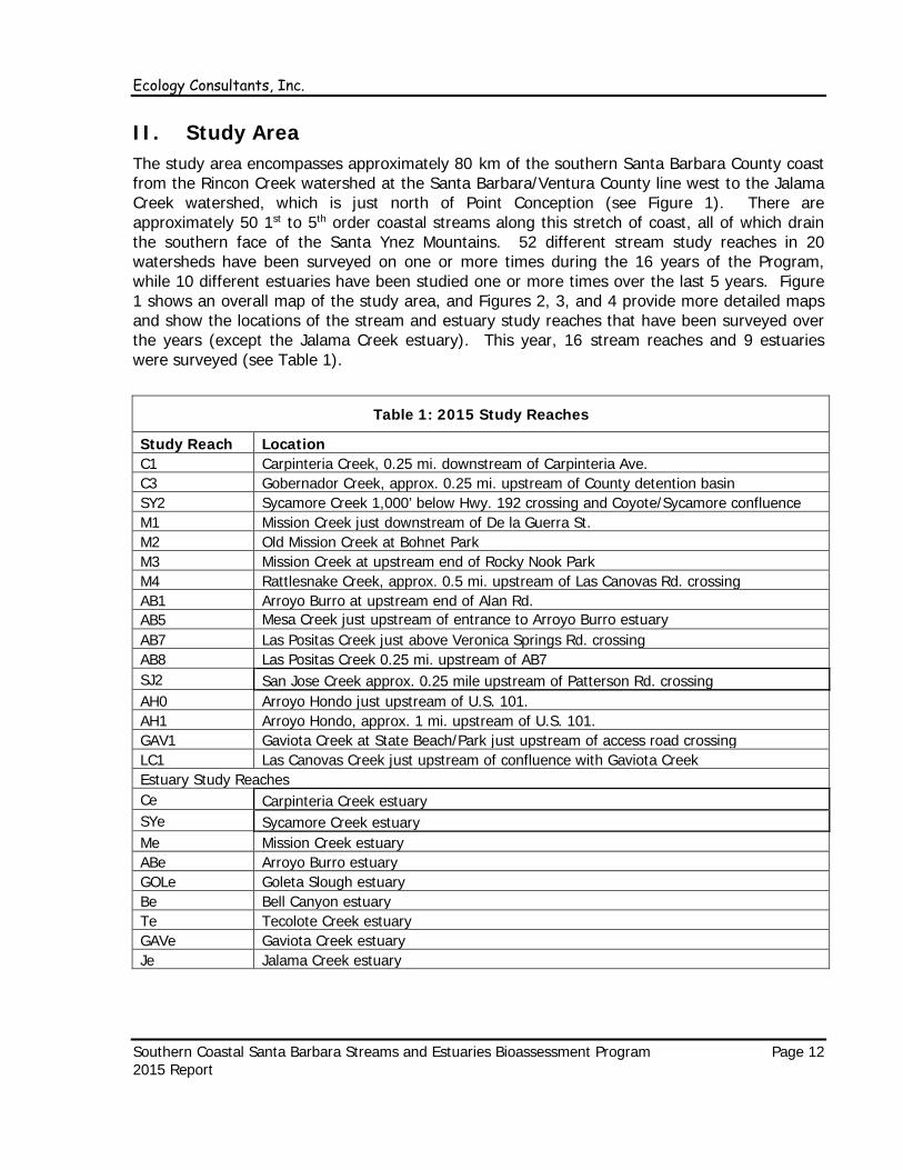
II. Study Area The study area encompasses approximately 80 km of the southern Santa Barbara County coast from the Rincon Creek watershed at the Santa Barbara/Ventura County line west to the Jalama Creek watershed, which is just north of Point Conception (see Figure 1). There are approximately 50 1st to 5th order coastal streams along this stretch of coast, all of which drain the southern face of the Santa Ynez Mountains. 52 different stream study reaches in 20 watersheds have been surveyed on one or more times during the 16 years of the Program, while 10 different estuaries have been studied one or more times over the last 5 years. Figure 1 shows an overall map of the study area, and Figures 2, 3, and 4 provide more detailed maps and show the locations of the stream and estuary study reaches that have been surveyed over the years (except the Jalama Creek estuary). This year, 16 stream reaches and 9 estuaries were surveyed (see Table 1).
Table 1: 2015 Study Reaches
Study Reach Location C1 Carpinteria Creek, 0.25 mi. downstream of Carpinteria Ave. C3 Gobernador Creek, approx. 0.25 mi. upstream of County detention basin SY2 Sycamore Creek 1,000’ below Hwy. 192 crossing and Coyote/Sycamore confluence M1 Mission Creek just downstream of De la Guerra St. M2 Old Mission Creek at Bohnet Park M3 Mission Creek at upstream end of Rocky Nook Park M4 Rattlesnake Creek, approx. 0.5 mi. upstream of Las Canovas Rd. crossing AB1 Arroyo Burro at upstream end of Alan Rd. AB5 Mesa Creek just upstream of entrance to Arroyo Burro estuary AB7 Las Positas Creek just above Veronica Springs Rd. crossing AB8 Las Positas Creek 0.25 mi. upstream of AB7 SJ2 San Jose Creek approx. 0.25 mile upstream of Patterson Rd. crossing AH0 Arroyo Hondo just upstream of U.S. 101. AH1 Arroyo Hondo, approx. 1 mi. upstream of U.S. 101. GAV1 Gaviota Creek at State Beach/Park just upstream of access road crossing LC1 Las Canovas Creek just upstream of confluence with Gaviota Creek Estuary Study Reaches Ce Carpinteria Creek estuary SYe Sycamore Creek estuary Me Mission Creek estuary ABe Arroyo Burro estuary GOLe Goleta Slough estuary Be Bell Canyon estuary Te Tecolote Creek estuary GAVe Gaviota Creek estuary Je Jalama Creek estuary

Ecology Consultants, Inc.
Southern Coastal Santa Barbara Streams and Estuaries Bioassessment Program Page 13 2015 Report
FIGURE 1: STUDY AREA
Source: Delorme Topoquads
N
Study Area

Ecology Consultants, Inc.
Southern Coastal Santa Barbara Streams and Estuaries Bioassessment Program Page 14 2015 Report
FIGURE 2: GAVIOTA COAST STUDY REACHES
SO2 AH1
San Onofre Creek
Arroyo Hondo
EC1
Refugio Creek
R2
R1 GAV1
Gaviota Creek
N
SO1
GAV2
AH2
Scale: 1 centimeter = 1 kilometer Source: Delorme Topoquads (1999) Study creeks emphasized for ease of recognition
San Onofre Creek
Arroyo Hondo Creek AH1
Refugio Creek
R2
R1
EC1
El Capitan Creek
SO2
GAVe R0
LC1
AH0

Ecology Consultants, Inc.
FIGURE 3: SANTA BARBARA AND GOLETA AREA STUDY REACHES
Southern Coastal Santa Barbara Streams and Estuaries Bioassessment Program Page 15 2015 Report
AT1
SJ1
SJ2
SJ3
AB2 AT2
N
San Jose Creek
Arroyo Burro
AB1 M1
M3
M2
Mission Creek SY1
Sycamore Creek
Scale: 1 centimeter = 1.5 kilometers Source: Delorme Topoquads (1999)
Atascadero Creek
San Antonio Creek
Maria Ygnacio Creek
MY1
SA1
Dos Pueblos Creek
DP1
T1
T3
Tecolote Creek
SJ4
MY2
MY3
SA2
M4
M6
M5
AB3
T2
AB7 AB8
AB5
AB6 SY2 AB4
ABe Me
SYe
Te Be
GOLe

Ecology Consultants, Inc.
Southern Coastal Santa Barbara Streams and Estuaries Bioassessment Program Page 16 2015 Report
FIGURE 4: CARPINTERIA AREA STUDY REACHES
N
RIN1
Scale: 1 centimeter = 2 kilometers
C1 C2
Carpinteria Creek
Rincon Creek
C3 AP1 F1
Santa Monica
Creek Franklin
Creek
Source: Delorme Topoquads (1999) Study streams emphasized for ease of recognition
Arroyo Paredon
Creek
SM1 RIN0 Ce

Ecology Consultants, Inc.
Southern Coastal Santa Barbara Streams and Estuaries Bioassessment Program Page 17 2015 Report
III. Methods
Physiochemical and biological data for the stream and estuary study reaches was gathered through a combination of methods including field surveys, laboratory analyses, spatial data analyses using geographic information system (GIS) software, and review of United States Geological Survey (USGS) 7.5-minute quadrangle maps and recent aerial photographs. BMI parameters were calculated from the raw data. Statistical tests including linear regressions and analyses of variance (ANOVA) were used to evaluate the streams and estuaries data for relationships with physiochemical parameters and measures of human disturbance. Further discussion of methods is provided below.
A. Field Surveys
1. Streams
Stream surveys involve annual collection of BMI samples and other pertinent physiochemical and biological data at study streams and estuaries using USEPA endorsed rapid bioassessment methodology. Our sampling methodology has been consistent since 2000, and is very similar to that currently used for the California Surface Water Ambient Monitoring Program (SWAMP), the methods of which have varied over the years. As in previous years of the Program, field surveys were conducted in the spring during base stream flow conditions (i.e., low flows). The sampling was conducted in May. Sampling in the spring during base flow conditions provides consistency in the sampling from year to year, as the local stream biota is known to undergo seasonal succession (Cooper et al., 1986). The following was completed during each field survey:
• General observations were recorded on a standardized field data sheet, including location, date, time, weather, stream flow conditions, water clarity, and human impacts.
• A 100-meter study reach was delineated along the stream. Stream habitat units (i.e., riffles, runs, pools, etc.) within the study reach were mapped and quantified as a percentage of the total reach length.
• Stream wetted and channel bottom width were measured at three transects in the study reach. The three transects were established at the 25, 50 and 75 meter marks. Wetted perimeter width is the cross-sectional distance of streambed that is inundated with surface water. Channel bottom width is the cross-sectional distance between the bottoms of the stream banks.
• Riparian canopy cover was estimated in the center of the stream channel at the three transects using a spherical densitometer.
• Plant and wildlife species observed in the stream and riparian zone were noted and recorded.
• Water temperature, conductance, pH, and dissolved oxygen concentration were measured in the field using YSI and Oakton handheld meters. Two measurements of each parameter were made, one in a riffle and the other in a pool, and the two values were averaged.

Ecology Consultants, Inc.
Southern Coastal Santa Barbara Streams and Estuaries Bioassessment Program Page 18 2015 Report
• One composite BMI sample was collected from each study reach using a standardized method based on the “multi-habitat” approach described in the USEPA’s Rapid Bioassessment Protocols for Use in Streams and Wadeable Rivers (Barbour et al., 1999). Each sample represents approximately one square meter of stream bottom, collected from 10 individual, 0.1-square meter locations (an approximately 30 cm square). The 10 locations that constituted the sample were selected based on the relative area each stream habitat (i.e., riffles, pools, falls, etc.) covered in the section of stream sampled. For example, if a stream reach contained approximately 50 percent riffles and 50 percent pools, five locations in riffles and five in pools were selected and sampled. Samples were collected using a D-frame net with 500 µm mesh. In locations with flowing water (e.g., riffles and runs), the net was held upright against the stream bottom, and substrata immediately upstream within the 0.1-square meter area was scraped and stirred up for approximately 15 seconds using feet and hands. Dislodged BMIs and stream bottom materials were carried into the net by the stream current. In areas with little or no current (e.g., pools), stream bottom material was stirred up by foot, followed by a quick sweep of the net through the water column to capture dislodged BMIs. This was repeated three times in each pool sampling location.
• After each BMI sample was collected, it was rinsed with water in a 500 µm sieve to wash out fine sediments, transferred to a plastic container, and preserved in 70 percent ethanol.
• A stream habitat assessment was completed using a new protocol developed by Ecology. The new protocol is similar to the U.S. EPA method used in previous years, but the habitat components and scoring criteria have been revised based on our 15 years of experience studying local streams. The old U.S. EPA provided a good basis to begin from, but some categories were redundant, and scoring criteria in some cases did not apply well to local streams. The new protocol yields a total score from 0 to 100 points for each study stream based on the assessment stream path and form (0-20), habitat diversity (0-10), habitat connectivity (0-10), hydrology (0-10), water column depth/velocity/quality (0-10), substrate/erosion/sedimentation (0-10), riparian vegetation cover/composition (0-10), riparian/upland buffer (0-10), and foot traffic/noise/lighting (0-10). The new habitat assessment is provided in the Appendix.
• Quality control measures were incorporated into the field surveys to insure accurate and consistent data gathering. Water monitoring equipment was calibrated regularly. Field crew members were trained to properly operate equipment, take measurements, collect BMI samples, and conduct stream habitat assessments.
2. Estuaries
Ecology conducted a rapid bioassessment survey in each study estuary in early October. Methodology was based on the Tier 1 approach described in Estuarine and Coastal Marine Waters: Bioassessment and Biocriteria Technical Guidance (Bowman et al., 2000). The Tier 1 approach is intended to provide an assessment of coastal wetland habitats based on sampling of one or more biological assemblages (e.g., algae, invertebrates, fish, etc.) and collecting data on water chemistry and bottom characteristics. The following was completed:
Ecology Consultants, Inc.
Southern Coastal Santa Barbara Streams and Estuaries Bioassessment Program Page 19 2015 Report
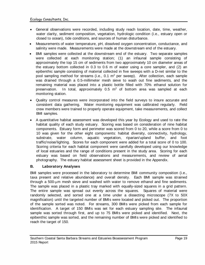
• General observations were recorded, including study reach location, date, time, weather, water clarity, sediment composition, vegetation, hydrologic condition (i.e., estuary open or closed to ocean), tide conditions, and sources of human disturbance.
• Measurements of water temperature, pH, dissolved oxygen concentration, conductance, and salinity were made. Measurements were made at the downstream end of the estuary.
• BMI samples were collected at the downstream end of the estuary. Two separate samples were collected at each monitoring station; (1) an infaunal sample consisting of approximately the top 15 cm of sediments from two approximately 10 cm diameter areas of the estuary bottom collected in 0.3 to 0.6 m of water using a core sampler, and (2) an epibenthic sample consisting of material collected in five sweeps with a D-net similar to the pool sampling method for streams (i.e., 0.1 m2 per sweep). After collection, each sample was drained through a 0.5-millimeter mesh sieve to wash out fine sediments, and the remaining material was placed into a plastic bottle filled with 70% ethanol solution for preservation. In total, approximately 0.5 m2 of bottom area was sampled at each monitoring station.
• Quality control measures were incorporated into the field surveys to insure accurate and consistent data gathering. Water monitoring equipment was calibrated regularly. Field crew members were trained to properly operate equipment, take measurements, and collect BMI samples.
• A quantitative habitat assessment was developed this year by Ecology and used to rate the habitat quality of each study estuary. Scoring was based on consideration of nine habitat components. Estuary form and perimeter was scored from 0 to 20, while a score from 0 to 10 was given for the other eight components: habitat diversity, connectivity, hydrology, substrate, water column, aquatic vegetation, riparian/upland buffer, and foot traffic/noise/lighting. Scores for each component were added for a total score of 0 to 100. Scoring criteria for each habitat component were carefully developed using our knowledge of local estuaries and the range of conditions present in the study area. Scoring for each estuary was based on field observations and measurements, and review of aerial photography. The estuary habitat assessment sheet is provided in the Appendix.
B. Laboratory Analyses
BMI samples were processed in the laboratory to determine BMI community composition (i.e., taxa present and relative abundance) and overall density. Each BMI sample was strained through a 500-µm mesh sieve and washed with water to remove ethanol and fine sediments. The sample was placed in a plastic tray marked with equally-sized squares in a grid pattern. The entire sample was spread out evenly across the squares. Squares of material were randomly selected, and sorted one at a time under a dissecting microscope (7X to 50X magnification) until the targeted number of BMIs were located and picked out. The proportion of the sample sorted was noted. For streams, 300 BMIs were picked from each sample for identification. A target of 150 BMIs was set for each estuary sampling site. The infaunal sample was sorted through first, and up to 75 BMIs were picked and identified. Next, the epibenthic sample was sorted, and the remaining number of BMIs were picked and identified to reach the target of 150.

Ecology Consultants, Inc.
Southern Coastal Santa Barbara Streams and Estuaries Bioassessment Program Page 20 2015 Report
BMIs were identified with the aid of taxonomic references including Merritt and Cummings (2008) and Smith and Carlton (1975). Insect taxa were identified to the family level. Non-insect taxa (e.g., oligochaetes, crustaceans, etc.) were typically identified to order or class. After sorting and identification, BMIs were bottled in 70 percent ethanol for storage. BMI sample processing methods were clearly established and strictly followed to ensure random selection and accurate enumeration and identification of BMIs.
C. GIS Analyses
GIS Arcview software was used to calculate upstream watershed area and watershed land use covers for each study reach. Watershed areas were calculated based on watershed boundaries generated in Arcview. Watershed land uses and percent cover for each study reach were calculated by superimposing watershed boundaries over a digital land cover GIS layer for the region. The land cover layer was produced the California Department of Forestry and Fire Protection’s (CDF) Fire and Resource Assessment Program (FRAP). The CDF land use map for the region showed coverage by the following eight land use categories: urban, agriculture, herbaceous, hardwood, shrub, conifer, water, and barren/other. Recent aerial photographs (2014 to 2015) of the region available on Google Earth were reviewed to refine the GIS land use layer.
The parameter “% watershed disturbed” was calculated for each study reach by using the following equation:
% watershed disturbed = % urban + % agriculture + 0.25(% herbaceous)
Herbaceous areas were counted as partially (i.e., a quarter) disturbed to reflect that much of the herbaceous lands in this region are used for livestock grazing or are previously cleared land. Such areas typically have lower habitat value and can contribute higher volumes of fine sediments to streams via erosion.
D. Review of Topographic Maps
USGS 7.5-minute quadrangle topographic maps (1:24,000 scale) for the study area were reviewed to determine stream order, elevation, and gradient for each study reach. Gradient was determined by dividing the elevation change between topographic contours immediately upstream and downstream of the study reach by the stream length between the contours. Stream length was determined by tracing a map wheel over the stream path.
E. Study Reach Grouping
Stream and estuary study reaches were placed into three different groups based on their level of human disturbance. These disturbance groups were assigned to study reaches “a priori”, or before the analyses of biological data, based on (1) physical habitat assessment scores, and (2) % upstream watershed disturbed. This approach allowed both reach and watershed scale impacts to be considered in the a priori assessment of habitat condition, both of which have been shown to be important predictors of BMI community composition in this and many other bioassessment studies. The following criteria are used to classify study reaches:
REF = Reaches that are in a “reference condition”, or are minimally to lightly disturbed by human activities. Habitat assessment score is 75/100 or greater, and no
Ecology Consultants, Inc.
Southern Coastal Santa Barbara Streams and Estuaries Bioassessment Program Page 21 2015 Report
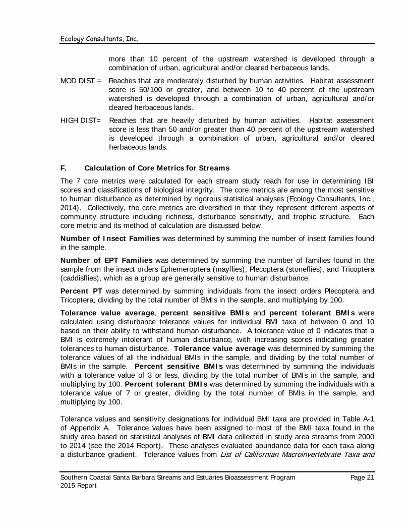
more than 10 percent of the upstream watershed is developed through a combination of urban, agricultural and/or cleared herbaceous lands.
MOD DIST = Reaches that are moderately disturbed by human activities. Habitat assessment score is 50/100 or greater, and between 10 to 40 percent of the upstream watershed is developed through a combination of urban, agricultural and/or cleared herbaceous lands.
HIGH DIST= Reaches that are heavily disturbed by human activities. Habitat assessment score is less than 50 and/or greater than 40 percent of the upstream watershed is developed through a combination of urban, agricultural and/or cleared herbaceous lands.
F. Calculation of Core Metrics for Streams
The 7 core metrics were calculated for each stream study reach for use in determining IBI scores and classifications of biological integrity. The core metrics are among the most sensitive to human disturbance as determined by rigorous statistical analyses (Ecology Consultants, Inc., 2014). Collectively, the core metrics are diversified in that they represent different aspects of community structure including richness, disturbance sensitivity, and trophic structure. Each core metric and its method of calculation are discussed below.
Number of Insect Families was determined by summing the number of insect families found in the sample.
Number of EPT Families was determined by summing the number of families found in the sample from the insect orders Ephemeroptera (mayflies), Plecoptera (stoneflies), and Tricoptera (caddisflies), which as a group are generally sensitive to human disturbance.
Percent PT was determined by summing individuals from the insect orders Plecoptera and Tricoptera, dividing by the total number of BMIs in the sample, and multiplying by 100.
Tolerance value average, percent sensitive BMIs and percent tolerant BMIs were calculated using disturbance tolerance values for individual BMI taxa of between 0 and 10 based on their ability to withstand human disturbance. A tolerance value of 0 indicates that a BMI is extremely intolerant of human disturbance, with increasing scores indicating greater tolerances to human disturbance. Tolerance value average was determined by summing the tolerance values of all the individual BMIs in the sample, and dividing by the total number of BMIs in the sample. Percent sensitive BMIs was determined by summing the individuals with a tolerance value of 3 or less, dividing by the total number of BMIs in the sample, and multiplying by 100. Percent tolerant BMIs was determined by summing the individuals with a tolerance value of 7 or greater, dividing by the total number of BMIs in the sample, and multiplying by 100.
Tolerance values and sensitivity designations for individual BMI taxa are provided in Table A-1 of Appendix A. Tolerance values have been assigned to most of the BMI taxa found in the study area based on statistical analyses of BMI data collected in study area streams from 2000 to 2014 (see the 2014 Report). These analyses evaluated abundance data for each taxa along a disturbance gradient. Tolerance values from List of Californian Macroinvertebrate Taxa and

Ecology Consultants, Inc.
Southern Coastal Santa Barbara Streams and Estuaries Bioassessment Program Page 22 2015 Report
Standard Taxonomic Effort (California Department of Fish and Game, 2002) were used for taxa that did not occur in sufficient abundance in local streams to allow for meaningful statistical analyses. 8 taxa that occur in the study area did not meet abundance criteria established in the 2014 analyses, nor did they have tolerance values in List of Californian Macroinvertebrate Taxa and Standard Taxonomic Effort. Thus, no tolerance values are provided for these taxa.
Percent predators + shredders was determined by summing individual BMIs with a predator or shedder functional feeding group designation, dividing by the total number of BMIs in the sample, and multiplying by 100. Functional feeding group designations were obtained from An Introduction to the Aquatic Insects of North America (Merritt and Cummins, 2008).
G. Core Metric Scoring Ranges for Streams
The IBI provides scoring ranges of between 0 and 10 for each of the seven core metrics (see Table 2). See the 2014 Report for discussion of how core metric scoring ranges were determined. For core metrics that decrease with increasing human disturbance (e.g., # insect families), higher values corresponded with higher scores. For core metrics that increase with increasing human disturbance (e.g., tolerance value average), lower values corresponded with higher scores.
Table 2: Core Metric Scoring Ranges
Score # EPT families
% sens BMIs TV Avg. # insect
families % shredders +predators %PT % tol BMIs
10 ≥15 ≥58 ≤3.62 ≥ 28 ≥ 25 ≥ 20 ≤ 16 9 14 44 to 57 3.63 to 4.40 26, 27 18 to 24 15 to 19 17 to 27 8 13 37 to 43 4.41 to 4.79 23 to 25 16, 17 13, 14 28 to 32 7 11, 12 29 to 36 4.80 to 5.18 21, 22 14, 15 10 to 12 33 to 37 6 9, 10 21 to 28 5.19 to 5.56 19, 20 12, 13 7 to 9 38 to 42 5 7, 8 17 to 20 5.57 to 5.91 17, 18 10, 11 5, 6 43 to 49 4 5, 6 12 to 16 5.92 to 6.26 15, 16 8, 9 4 50 to 57 3 4 7 to 11 6.27 to 6.60 13, 14 6, 7 3 58 to 65 2 3 2 to 6 6.61 to 6.93 11, 12 4, 5 2 66 to 73 1 2 1 6.94 to 7.53 6 to 10 3, 4 1 74 to 90 0 0, 1 0 ≥7.54 ≤ 5 ≤ 1 0 ≥ 91
H. IBI Classifications of Biological Integrity and Scoring Ranges for Streams
Individual scores for the 7 core metrics are summed to provide a total score of between 0 and 70 for the study reach. The IBI provides 5 classifications of biological integrity based on the total score: Excellent, Good, Fair, Poor, and Very Poor. IBI classifications and scoring ranges are provided in Table 3. See the 2014 report for discussion of how ranges were set for the 5 classifications of biological integrity.

Ecology Consultants, Inc.
Southern Coastal Santa Barbara Streams and Estuaries Bioassessment Program Page 23 2015 Report
Table 3 IBI Classifications of Biological Integrity (Streams)
Category Scoring Range
Excellent 59 to 70
Good 46 to 58
Fair 29 to 45
Poor 11 to 28
Very Poor 0 to 10
I. Data Analyses for Streams
Individual Streams Study Reaches
A discussion of each stream study reach is provided, including physiochemical conditions, biological data, and IBI scores as determined through field surveys, lab work, and review of maps, aerial photos, and GIS. Study stream photographs are provided, as are graphs to illustrate IBI score trends through time.
Drought Effects
Analyses in previous years have shown significant negative effects to streams BMI communities and IBI scores following natural episodic disturbances including (1) very high rainfall and peak stream flows that occurred in winter 2004/2005, and (2) major wildfires including the Gaviota (2004), Gap (2008), Tea (2008), and Jesusita (2009) fires. In general, BMI communities recovered within a year or two following the extreme flows and fires. More recently (i.e., last year), negative effects to streams BMI communities and downward trends in IBI scores became evident in response to the current prolonged drought, which has reached 4 years in duration. While most of the stream study reaches have maintained perennial flow during drought periods that lasted a year or two, many have experienced partial or complete drying of riffles and even pools for substantial lengths of time over the past two years.
Last year’s analyses showed a downward trend in stream IBI scores in 2013, and even more so in 2014 in response to the ongoing drought. As the drought continued this year, it was anticipated that the downward trend on streams IBI scores would continue as well. Analyses of Variance (ANOVAs) were used to explore the nature and strength of relationships between stream flow at individual study reaches and IBI scores, core metrics, and other BMI parameters. Study reaches were partitioned into stream flow groups based on the following criteria:
1. (F-F): Flowing in spring, flowing the previous fall 2. (F-P): Flowing in spring, pools only or dry previous fall 3. (P-P): Pools only in spring, pools only or dry previous fall
An ANOVA compares the means and distributions of a given metric among multiple sampling groups, and indicates the probability that the means for the groups are the same. The probability that the means are the same is expressed as p, which is between 0 and 1. The lower the p, the lower the probability that the group means are the same. A p of 0.05 (i.e.,

Ecology Consultants, Inc.
Southern Coastal Santa Barbara Streams and Estuaries Bioassessment Program Page 24 2015 Report
5%) or less is generally accepted as indicating a statistically significant difference between group means.
Replicates for the ANOVAs included stream study reaches from 2012 to 2015, as we began making fall (late September or early October) observations of stream study reaches in 2011. ANOVAs were completed separately by disturbance group (i.e., REF, MOD DIST, and HIGH DIST) to account for the fact that human disturbance can greatly influence the BMI community, and was expected to mask any effects of drought at HIGH DIST and possibly at MOD DIST streams.
Year-to-Year Trends in IBI Scores
ANOVAs were completed to compare IBI scores for the 3 disturbance groups (REF, MOD DIST, and HIGH DIST) to see whether the IBI differentiated between disturbance groups this year and in the past. ANOVAs were also competed to compare IBI scores for REF study reaches for individual years from 2000 to 2015.
J. Calculation of BMI Metrics for Estuaries
14 BMI metrics were calculated for the study estuaries, including measures of abundance, diversity, disturbance sensitivity, and trophic structure (see Table 2). Many of the metrics calculated are similar to some used effectively as indicators of biological condition in one or more recent estuarine studies conducted throughout the nation.
Table 4: BMI Metrics Calculated for Study Estuaries
BMI Metric Abbreviation Units of Measurement
Method of Calculation
BMI density None # per m2 Lab # of taxa # taxa None Lab # of sensitive taxa # sens taxa None Lab # of tolerant taxa # tol taxa None Lab # sensitive taxa/# tolerant taxa # sens/ # tol None Lab % sensitive BMIs % sens BMIs % Lab % tolerant BMIs % tol BMIs % Lab % insects None % Lab % non-insects None % Lab % dominant taxon None % Lab % 2 dominant taxa None % Lab % predators % pred % Lab % collector-gatherers % cg % Lab 100+(%collector-gatherers – %predators) 100+(%cg-%pred) % Lab
BMI density (number of individuals per m2) was calculated by dividing the number of specimens picked out of the sample by the subsampled area. Richness parameters were determined by counting the number of specified taxa identified in each sample. % sensitive BMIs, and % tolerant BMIs were calculated by adding the number of BMIs in the sample labeled as either “sensitive” or “tolerant” to human disturbance, dividing by the total number of individuals in the sample, and multiplying by 100. # sensitive taxa and # tolerant taxa were calculated by adding
Ecology Consultants, Inc.
Southern Coastal Santa Barbara Streams and Estuaries Bioassessment Program Page 25 2015 Report
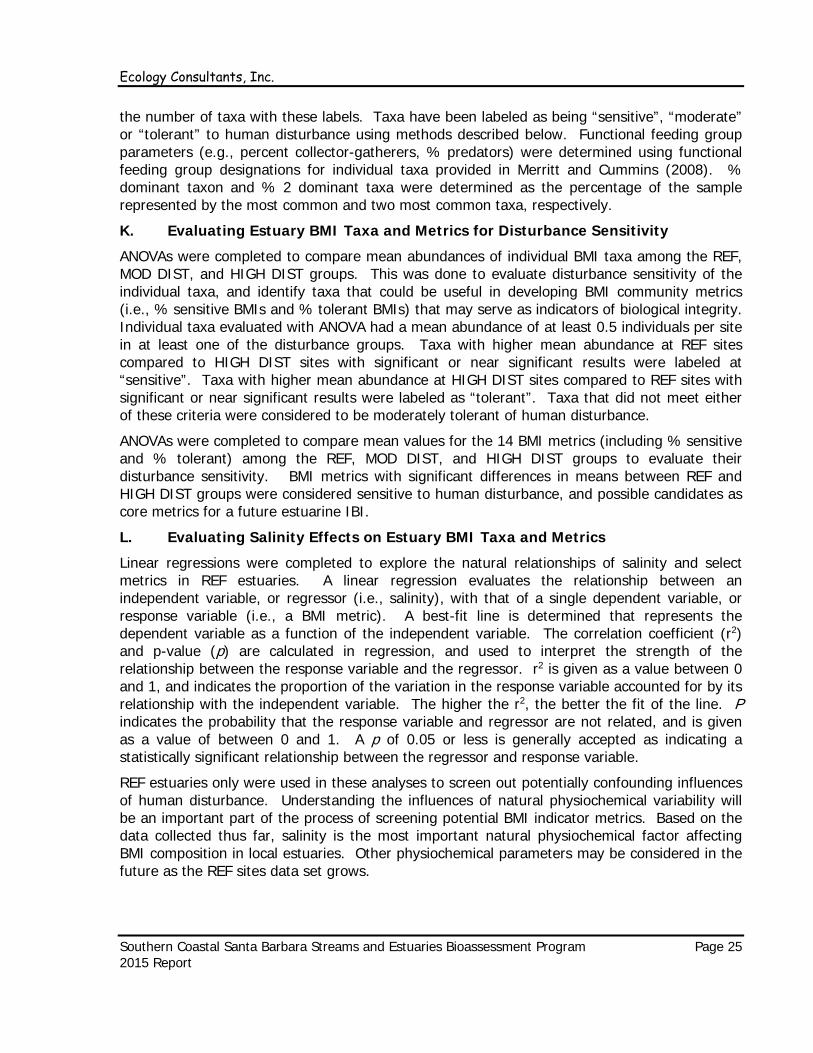
the number of taxa with these labels. Taxa have been labeled as being “sensitive”, “moderate” or “tolerant” to human disturbance using methods described below. Functional feeding group parameters (e.g., percent collector-gatherers, % predators) were determined using functional feeding group designations for individual taxa provided in Merritt and Cummins (2008). % dominant taxon and % 2 dominant taxa were determined as the percentage of the sample represented by the most common and two most common taxa, respectively.
K. Evaluating Estuary BMI Taxa and Metrics for Disturbance Sensitivity
ANOVAs were completed to compare mean abundances of individual BMI taxa among the REF, MOD DIST, and HIGH DIST groups. This was done to evaluate disturbance sensitivity of the individual taxa, and identify taxa that could be useful in developing BMI community metrics (i.e., % sensitive BMIs and % tolerant BMIs) that may serve as indicators of biological integrity. Individual taxa evaluated with ANOVA had a mean abundance of at least 0.5 individuals per site in at least one of the disturbance groups. Taxa with higher mean abundance at REF sites compared to HIGH DIST sites with significant or near significant results were labeled at “sensitive”. Taxa with higher mean abundance at HIGH DIST sites compared to REF sites with significant or near significant results were labeled as “tolerant”. Taxa that did not meet either of these criteria were considered to be moderately tolerant of human disturbance.
ANOVAs were completed to compare mean values for the 14 BMI metrics (including % sensitive and % tolerant) among the REF, MOD DIST, and HIGH DIST groups to evaluate their disturbance sensitivity. BMI metrics with significant differences in means between REF and HIGH DIST groups were considered sensitive to human disturbance, and possible candidates as core metrics for a future estuarine IBI.
L. Evaluating Salinity Effects on Estuary BMI Taxa and Metrics
Linear regressions were completed to explore the natural relationships of salinity and select metrics in REF estuaries. A linear regression evaluates the relationship between an independent variable, or regressor (i.e., salinity), with that of a single dependent variable, or response variable (i.e., a BMI metric). A best-fit line is determined that represents the dependent variable as a function of the independent variable. The correlation coefficient (r2) and p-value (p) are calculated in regression, and used to interpret the strength of the relationship between the response variable and the regressor. r2 is given as a value between 0 and 1, and indicates the proportion of the variation in the response variable accounted for by its relationship with the independent variable. The higher the r2, the better the fit of the line. P indicates the probability that the response variable and regressor are not related, and is given as a value of between 0 and 1. A p of 0.05 or less is generally accepted as indicating a statistically significant relationship between the regressor and response variable.
REF estuaries only were used in these analyses to screen out potentially confounding influences of human disturbance. Understanding the influences of natural physiochemical variability will be an important part of the process of screening potential BMI indicator metrics. Based on the data collected thus far, salinity is the most important natural physiochemical factor affecting BMI composition in local estuaries. Other physiochemical parameters may be considered in the future as the REF sites data set grows.

Ecology Consultants, Inc.
Southern Coastal Santa Barbara Streams and Estuaries Bioassessment Program Page 26 2015 Report
IV. Results and Discussion
A. Physiochemical and Biological Data
Table A-1 in the Appendix provides physiochemical data collected at the streams this year and in previous years of study. Table A-1 also lists BMI taxa and abundances for each stream studied, as well as BMI density, core metric values, and IBI score. Tolerance values and functional feeding groups are provided for individual BMI taxa. Table A-2 provides a list of the plant species observed at each stream, and the number and percentage of native vs. introduced plant species observed. Table A-3 provides a list of vertebrate species observed at the streams. For streams that have been surveyed multiple times, plant and vertebrate species observations are combined. Table A-4 provides physiochemical and BMI data and metrics for study estuaries.
B. Streams
1. Stream Study Reaches
The following discusses IBI scores at the individual streams for 2015, and compares this year’s scores to previous years. Physical habitat conditions, rainfall and stream flow patterns, and other factors that have likely affected the stream biota are also discussed.
Carpinteria Creek Watershed
C1 is located in lower Carpinteria Creek just downstream of the 8th St. pedestrian bridge at an elevation of 15’. Gradient is low at 0.01. This is a MOD DIST reach, with 80% undisturbed, 17% agricultural, and 3% agricultural lands in its upstream watershed of 9,598 acres. Peak elevation in the Carpinteria Creek watershed is approximately 4,700’. Habitat assessment score was 55 this year, and has ranged from 50 to 63 in 15 years of study. C1 is abutted by residential neighborhoods and vacant fields, and has natural soil banks with some loose riprap and old pipe and wire revetment present. The streambed is composed of small boulders, cobble, gravel, and sand, and normally has gentle riffles and 0.5-3’ deep pools. Flow was very low but continuous through C1, with slow narrow riffles, and pools that were showing signs of stagnation. The riparian corridor was 30-60’ in width, containing many mature cottonwoods and sycamores of 50’ or more in height, and a generally dense understory. Due to a lack of scouring flows, emergent vegetation, primarily horsetails (Equisetum spp.) and watercress (Rorippa nasturtium-aquaticum), have established in much of the streambed. 63% of the 56 plant species recorded at C1 are native. Riparian canopy cover was 90%, and has ranged from 50 to 90%. Lower Carpinteria Creek is moderately fragmented from the upper mainstem and tributaries by partial barriers at
C1 (above) and C3 (below): Low but continuous flow, natural boulder/cobble substrate, stream channel is thick with vegetation due to lack of scouring.

Ecology Consultants, Inc.
Southern Coastal Santa Barbara Streams and Estuaries Bioassessment Program Page 27 2015 Report
U.S. 101 and other road crossings and debris basins. Noise, lighting, and human traffic impacts at C1 are moderate.
C3 is in Gobernador Creek (Carpinteria Creek tributary) ¼-mile upstream of the debris basin at an elevation of 420’. C3 is a REF study reach, with an upstream watershed of 4,517 acres of 100% undisturbed wilderness lands and peak elevation of approximately 4,700’. Human disturbances upstream of C3 are limited to dirt roads and cattle ranching. In the past there was a 2” metal pipe running down the stream indicating a possible surface water diversion, but these were washed out. It is unknown if there are currently any major surface water withdrawals from the stream. This section of Gobernador Creek has moderate gradient (0.03) and passes through a narrow gorge. Canyon walls are composed of exposed bedrock and soil slopes, and the streambed is formed in the bedrock with large boulders, small boulders, cobble, gravel, and sand substrate. Riffles and cascades alternate with pools of varying sizes and depths of 1’ to 4’. Flow was low but continuous through C3 this year, and flow has typically been perennial over the years. Overall, stream habitat is excellent, as reflected by a habitat assessment score of 85 this year, ranging from 85 to 93 in 15 years of study. The riparian corridor is dense and dominated by mature white alders (Alnus rhombifolia), sycamores, and coast live oaks, with riparian canopy cover of 95% this year and range of 70-100% overall. While 83% of the 69 plant species recorded at C3 are native, approximately 30-40% of the riparian understory cover is non-native, mostly thoroughwort (Ageratina ademorpha) and cape ivy (Senecio mikanioides). Due to a lack of scouring flows, emergent vegetation, primarily horsetails and thoroughwort, were established in much of the streambed this spring.
C1 had favorable water temperature (17.0 ºC), pH (7.6) and dissolved oxygen (6.7 mg/l), but elevated specific conductance (1,821 µS), likely indicating that there are pollution inputs (i.e., increased ionic dissolved solids) from agricultural and urban runoff. In the past specific conductance typically has been in the 1,200-1,800 µS range. C3 also had favorable water temperature (13.4 ºC), pH (7.9) and dissolved oxygen (8.2 mg/l). Specific conductance was much lower (1,120 µS) than at C1, yet the highest it has been in 15 years of study at C3, where it has typically been in the 600-800 µS range. The previous high was 1,000 µS last year. The higher mineral content in the water is presumably a side effect of the prolonged drought, which has resulted less contribution of relatively diluted rainwater to surface flows, and concentration of dissolved minerals in the shallow groundwater deposits that feed surface flows in the dry season.
IBI score at C1 was 5 (Very Poor), and within the range (0 to 19) from 15 years of study (see Figure 5). The consistently low IBI scores for C1 over the years are puzzling. This site has good substrate dominated by cobble, gravel, and sand, well-defined riffles and pools, natural banks and a decent riparian corridor with numerous mature canopy trees. The basic water quality parameters measured have shown signs of disturbance in the form of moderately high conductivity and somewhat variable dissolved oxygen, but not alarmingly so. The watershed has little urban use (3%), some agriculture (17%), and is mostly undisturbed wilderness (80%). Other sites such as SJ2, AB1, and SY2 with similar or greater habitat disturbances have consistently had higher IBI scores compared to C1. A likely contributor to low IBI scores at C1 is a lack of flowing water in the dry season in low rainfall years. This site has always been wet in fall observations, but last September (2014), while it had pools, there was no visible flow, and dissolved oxygen was very low at 2.0 mg/l. Similar conditions were observed in September

Ecology Consultants, Inc.
Southern Coastal Santa Barbara Streams and Estuaries Bioassessment Program Page 28 2015 Report
2013 as well. Lack of flow and dissolved oxygen crashes in the dry season could be responsible for a loss of many BMI taxa in drought years. However, the BMI community at C1 has been depauparate as well following wet years when flow has been perennial, which would allow establishment of a more diverse BMI community in a healthier stream. More detailed analyses of the water chemistry at C1 and determination of upstream water pollutant sources may shed light on other causes of biological impairment at C1.
IBI score was 14, Poor at C3 this year, the lowest in 15 years of study at this site (see Figure 5). IBI score was also Poor last year (24). C3 is a REF stream that typically scores in the Good to Excellent range. C3 had only standing pools in September 2013 and 2014, presumably with low dissolved oxygen levels. The past 2 years C3 has been characterized by much lower than normal EPT and insect family richness, and a higher proportion of tolerant BMIs, mostly Chironomidae, which made up over 60% of the sample this year. Similar patterns have been observed in other REF and MOD DIST stream reaches including M3, M4 and AB3 that dried in the dry season in drought years.
30 vertebrate species have been observed over the years at C1, including 2 aquatic species: Pacific tree frogs (Psuedacris regilla) and three-spine sticklebacks (Gasterosteus acleatus). At C3, 37 vertebrate species have been observed, including 5 aquatic species: rainbow trout (Oncorhynchus mykiss) and California newts (Taricha torosa), both observed in large numbers in most years, and two-striped garter snake (Thamnophis hammondii), California tree frog (Pseudacris cadaverina), and Pacific tree frog. However, no trout have been observed at C3 the last 2 years, presumably due to drying over the last couple of summers due to the drought.
01020304050607080
2000 2001 2002 2003 2004 2005 2006 2007 2008 2009 2010 2011 2012 2013 2014 2015
IBI S
core
Year
Figure 5: Carpinteria Creek Watershed IBI Scores
C1
C3

Ecology Consultants, Inc.
Southern Coastal Santa Barbara Streams and Estuaries Bioassessment Program Page 29 2015 Report
Sycamore Creek Watershed
SY1, located in lower Sycamore Creek just downstream of Mason St., was completely dry for the second straight year and therefore was not surveyed. SY2 is located in the foothills near the middle of the Sycamore Creek watershed at an elevation of 170’ above sea level. Gradient is moderate at 0.03. This is HIGH DIST reach due to its high level of watershed development, with 52% undisturbed, 46% urban, and 2% agricultural lands in its upstream watershed of 1,956 acres. Peak elevation in the Sycamore Creek watershed is approximately 2,100’. Habitat assessment score was 65 this year, and has ranged from 55 to 68 in 12 years of study. Just above its banks SY2 is tightly abutted by Sycamore Cyn. Rd. on its east, and a steep slope planted with avocados to the west, with homes tightly abutting the stream upstream and downstream of SY2. Several driveways cross the stream upstream and downstream of SY2, the bridges having grade drops that act as significant movement barriers, fragmenting the stream habitat. The stream has mostly natural bedrock and boulder bed and banks, with steep riffles, cascades, falls, and pools. There is some riprap and asphalt debris in the stream channel. As in previous years, high levels of fine sediments were present, partially filling pools and moderately to highly embedding much of the riffle cobbles and gravels. Sources of fine sediments include erosional areas from large landslides in the upper canyons and middle reaches, particularly where Sycamore Creek and its tributaries cut through Monterey and Rincon shale formations. Past residential lot grading without proper erosion control measures in the upper watershed also contributes to erosion problems (Questa, 2005).
Stream flow was very low but continuous throughout SY2 during this year’s spring survey, showing the effects of the 4-year drought. Riffles were very shallow (1” or less deep) and narrow (less than 1’) but were flowing. Pools were generally narrower and shallower compared to wetter years, ranging in depth from 0.5’ to 2.0’. The stream banks support a narrow corridor of mostly native riparian vegetation with a canopy dominated by mature sycamore (Plantanus racemosa), coast live oak (Quercus agrifolia), and willows (Salix spp.). Riparian canopy cover was 90%, and has ranged from 72 to 100% in previous years. Due to the absence of significant scouring flows, the stream channel has become choked with emergent herbaceous plants and riparian vines, mostly horsetail, Poison oak (Toxicodendron diversilobum), and California blackberry (Rubus urinus). 46% of the 41 plant species recorded at SY2 are native. Human impacts at the site include noise and lighting from the Sycamore Cyn. Rd. and nearby homes, and human traffic in the streambed and banks as evidenced by
SY2: upstream view
SY2: vegetated streambed
SY2: Red-eared slider
Ecology Consultants, Inc.
Southern Coastal Santa Barbara Streams and Estuaries Bioassessment Program Page 30 2015 Report
trampling of riparian vegetation and the presence of bottles and other trash.
Water chemistry measurements at SY2 were typical of previous years, with low water temperature (14.6ºC), adequate dissolved oxygen (6.3 mg/l), and high specific conductance (2,282 µS). Over the years, Sycamore Creek study reaches have had consistently higher conductance compared study reaches in other nearby watersheds (e.g., Mission Creek, Arroyo Burro, Montecito Creek), with similar human development patterns. While high stream conductance is a common symptom of pollutant loading from human sources, it can also be due to naturally high mineral content in shallow groundwater, which varies considerably in mineral content locally due to influences of surrounding bedrock (Questa, 2005). In the case of Sycamore Creek, both natural and human factors almost certainly contribute to high conductivity.
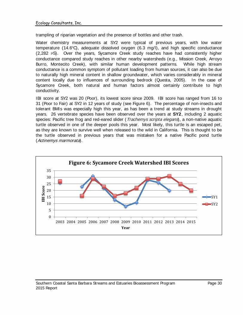
IBI score at SY2 was 20 (Poor), its lowest score since 2009. IBI score has ranged from 16 to 31 (Poor to Fair) at SY2 in 12 years of study (see Figure 6). The percentage of non-insects and tolerant BMIs was especially high this year, as has been a trend at study streams in drought years. 26 vertebrate species have been observed over the years at SY2, including 2 aquatic species: Pacific tree frog and red-eared slider (Trachemys scripta elegans), a non-native aquatic turtle observed in one of the deeper pools this year. Most likely, this turtle is an escaped pet, as they are known to survive well when released to the wild in California. This is thought to be the turtle observed in previous years that was mistaken for a native Pacific pond turtle (Actinemys marmorata).
05
101520253035
2003 2004 2005 2006 2007 2008 2009 2010 2011 2012 2013 2014 2015
IBI S
core
Year
Figure 6: Sycamore Creek Watershed IBI Scores
SY1
SY2

Ecology Consultants, Inc.
Southern Coastal Santa Barbara Streams and Estuaries Bioassessment Program Page 31 2015 Report
Mission Creek Watershed
M1 is located in lower Mission Creek just downstream of De la Guerra St. at an elevation of 40’. Gradient is low at 0.01. This is a HIGH DIST reach, with 49% undisturbed, 49% urban, and 2% agricultural lands in its upstream watershed of 6,799 acres. Peak elevation in the Mission Creek watershed is approximately 4,000’. Habitat assessment score was 23 this year, and has ranged from 23 to 35 in 15 years of study. M1 is tightly abutted by homes and commercial uses along both of its banks, which are composed mostly of hard concrete walls, with rip rap armored earth banks in sections. The streambed is composed of cobble, gravel, and sand, and normally has gentle riffles and 0.5’ to 3’ deep pools. Riffle areas were dry this year, with residual pools present. The patchy riparian canopy at M1 was limited to a few mature sycamores, white alders and ornamental trees. Riparian canopy cover was 68%, and has ranged from 28 to 71%. Riparian understory herbs, vines, and grasses were thick in the streambed. 47% of the 43 plant species recorded at M1 are native. The habitat of lower Mission Creek is severely constrained and fragmented by adjacent urban development, road crossings, and the ½-mile long concrete channel beginning just upstream of M1. Noise, lighting, and human traffic impacts to the stream are high. M2 is located in the old Mission Creek channel at Bohnet Park at 50’ in elevation. Gradient is low at 0.02. This is a HIGH DIST reach, with 24% undisturbed and 76% urban lands in its upstream watershed of 643 acres with a peak elevation of 400’. Old Mission Creek, which historically was the main channel of Mission Creek, was cut off and replaced by the concrete channel north of U.S. 101 during the construction of the highway. Old Mission Creek now receives runoff only from urban areas and natural slopes of the Santa Barbara west side. Habitat assessment score at M2 was 40 this year, and has ranged from 20 to 45 in 12 years of study. Bohnet Park buffers the stream on both sides from nearby residential and commercial development. M2 has earthen, highly erodable banks that are armored with chain link curtains and large boulders in sections. The streambed is composed of angular cobble, gravel, sand, and finer sediments and has gentle riffles and shallow, small pools that are 0.5’ to 1’ deep and 4’ to 6’ wide. Stream flow was low but continuous through M2 this year, and stronger than at most study reaches. The riparian corridor has benefited from plantings of native species in 2002. The dense riparian canopy is dominated by maturing willows, sycamores, white alders, and black cottonwoods (Populus balsamifera trichocarpa) 20
M1: standing pools
M1: dry riffles
M2: continuous flow, riffle and pool habitat intact

Ecology Consultants, Inc.
Southern Coastal Santa Barbara Streams and Estuaries Bioassessment Program Page 32 2015 Report
to 40 feet high. Riparian canopy cover was 91% this year, and has ranged from 18 to 95%. Riparian understory herbs, vines, and grasses are somewhat patchy. 71% of the 52 plant species recorded at M2 are native. The restoration project also included the development of an upstream oxbow (i.e., bend) and bioswale intended to filter urban storm water, and later an ultraviolet disinfection system to reduce bacteria levels in the water. Besides storm water, the stream regularly receives surface flows from groundwater pumping. Noise, lighting, and human traffic impacts to the stream are high due to the popularity of Bohnet Park and the density of nearby development. M3 is located in upper Mission Creek at Rocky Nook Park at 400 feet in elevation. Gradient is high at 0.07. This is a MOD DIST reach, with 80% undisturbed, 18% suburban, and 2% agricultural lands in its upstream watershed of 4,142 acres. Peak elevation in M3’s watershed is approximately 4,000’. Habitat assessment score was 80 this year, and has ranged from 68 to 85 in 14 years of study. Other than day use areas and trails from Rocky Nook Park, M3 is immediately adjoined by a natural floodplain, natural rock and soil banks, and natural boulder-dominated streambed with riffles, cascades/falls and plunge pools. The streambed contains clean cobble and gravel deposits ideal for rainbow/steelhead trout spawning, and sand and fine sediment deposits in pools. This year stream flow at M3 was continuous but very low in riffles and cascades, and pools ranged from 0.5’ to 2’ deep. The riparian canopy at M3 is dominated by mature sycamore, coast live oak, and white alder. Riparian canopy cover was 93%, and has ranged from 85% to 99%. Riparian understory herbs, vines, and grasses were dense in the streambed due to the lack of scouring flows. 72% of the 60 plant species recorded at M3 are native. The habitat of upper Mission Creek is fragmented by several road crossings and grade drops. Noise, lighting, and human traffic impacts to the stream are moderate due to the popularity of Rocky Nook Park and nearby roads. M4 is located in Rattlesnake Creek, a tributary of upper Mission Creek that drains the Rattlesnake Canyon wilderness area. M4 is at 1,000 feet in elevation, and has a high gradient of 0.08. This is a REF reach, with 98% undisturbed and 2% suburban lands in its upstream watershed of 1,376 acres. Peak elevation in the watershed is approximately 3,700’. Habitat assessment score was 85 this year, and has ranged from 73 to 95 in 10 years of study. M4 flows through a narrow, natural canyon and has steep rock and soil banks, and a natural streambed formed in bedrock and boulders with riffles, cascades, falls and plunge pools. Substrate is similar to M3, and is also ideal for rainbow/steelhead trout spawning when sufficient flow is present. This year stream flow at M4 was not continuous. There was very low flow in some riffles, but other sections were dry, thus pools were isolated and stagnant. Pools ranged from 1’ to 3’ deep. The dense riparian canopy is composed of mature sycamore, coast
M3: Watercress fills the channel due to low flow
M4: old rock dam eroding, residual plunge pool

Ecology Consultants, Inc.
Southern Coastal Santa Barbara Streams and Estuaries Bioassessment Program Page 33 2015 Report
live oak, and white alder. Riparian canopy cover was 98%, and has ranged from 93% to 100%. Riparian understory herbs, vines, and grasses are sparse due to heavy shading and near vertical bedrock canyon walls. 97% of the 38 plant species recorded at M4 are native. Rattlesnake Creek is fragmented by a large debris dam ¼-mile downstream of M4, which is a migration barrier to some aquatic species. The remains of an old rock dam create a waterfall 5’ high at the upper end of M4, although this impediment is eroding and was 15’ high just a few years ago, and there are several natural falls upstream. Noise, lighting, and human traffic impacts to the stream are low at M4 due to its limited accessibility.
M1 had lower than normal water temperature (16.0 ºC) and pH (7.4), and moderate specific conductance (1,193 µS). Dissolved oxygen was very low (2.2 mg/l) in residual pools due to the lack of stream flow and circulation. M2, which had continuous stream flow, had similar water chemistry readings as in previous years, with moderate temperature (18.9 ºC) and pH (8.2), optimal dissolved oxygen (9.8 mg/l), and elevated specific conductance (1,267 µS). Both M1 and M2 are subject to significant pollutant inputs from urban runoff. M3, which had continuous flow, had similar water temperature (15.6 ºC), dissolved oxygen (9.2 mg/l), pH (7.9) and specific conductance (1,148 µS) compared to previous years. Water quality is generally good at this site, with only minor pollution inputs expected due to the low level of development upstream. M4, which was limited to standing pools this year, had similar temperature (15.6 ºC), pH (7.4) and specific conductance (956 µS) compared to previous years, but like M1 had very low dissolved oxygen (2.5 mg/l) due to a lack of surface flow and circulation.
IBI score at M1 was 0 (Very Poor) this year, and 9 (Very Poor) at M2 (see Figure 7). IBI score has been in the Very Poor or lower Poor range at both sites over the years. These sites are both characterized by low proportion of sensitive taxa, EPT taxa, predators and shredders, low EPT and insect richness, and high proportion of tolerant taxa. As was case this year, M2 typically scores slightly better than M1. IBI score at M3 was 32 (Fair), which is on the lower end for this study reach, which typically scores from Fair to Good. Low flow levels and drying over last summer is a probable cause of lower IBI score, as M3 had only standing pools in September 2014. IBI score at M4 was 4 (Very Poor) this year, which is a drastic drop from last year, when the stream scored 48 (Good). M4 is a REF study reach and typically scores in the Good to Excellent range. The prolonged drought has severely impacted this study reach, which had only standing pools last September (2014), and at the time of this year’s spring survey. The lack of riffle habitat and extremely low dissolved oxygen levels in residual pools created inhospitable conditions this year for many BMI taxa that typically inhabit M4. The effects of the drought on M4 are even more dramatic than those of the Jesusita Fire of 2009, which burned the majority of the upper Mission Creek watershed, and coupled with erosive flood flows the following winter caused a drastic drop in IBI scores at M4 (13, Poor) and M3 (20, Poor) the following spring.
A total of 25, 24, 29, and 21 vertebrate species have been observed over the years at M1, M2, M3, and M4. Pacific tree frogs have been observed at all 4 study reaches. Three-spined stickleback and mosquitofish (non-native) have been observed at M1. California newts (Taricha torosa) were observed at M4 this year, but not at M3. Rainbow trout were not observed at M3 or M4 this year. Newts and trout were regularly observed at both M3 and M4 in the past. Trout have not been seen at either study reach since the Jesusita Fire in May 2009, which combined with strong scouring flows and erosion the following winter devastated the landscape

Ecology Consultants, Inc.
Southern Coastal Santa Barbara Streams and Estuaries Bioassessment Program Page 34 2015 Report
and stream community. While the BMI community and California newt populations appeared to recover from the fire effects over 2 to 3 years, trout have not recolonized M3 or M4. California tree frog (Pseudacris cadaverina) has been observed at M4.
Arroyo Burro Watershed
AB1 is located in lower Arroyo Burro just upstream of the north end of Alan Rd. at an elevation of 25’. Gradient is low at 0.01. This HIGH DIST reach has 51% undisturbed, 38% urban, 7% agricultural and 4% herbaceous lands in its upstream watershed of 5,646 acres. Peak elevation in the Arroyo Burro watershed is approximately 4,000’. Habitat assessment score was 55 this year, ranging from 53 to 55 in 13 years of study. AB1 is bordered by vacant land and natural hills to the west, and a 75-100’ wide riparian/upland buffer and Las Positas Rd. to the east. Stream banks are moderately steep and sandy, and stream flow was continuous through gentle cobble and gravel riffles and sand-bottomed pools 1’ to 4’ deep. Lower Arroyo Burro, fed by Veronica Springs, is among the most consistent perennial streams in the study area. The patchy riparian canopy at AB1 is mostly willows, with a few coast live oaks and young sycamores and white alders. There are also stands of invasive non-native Arundo donax. Riparian canopy cover was 85% this year, and has ranged from 40% to 97%. Riparian understory herbs, vines, and grasses were dense in the streambed and banks. 54% of the 56 plant species recorded at AB1 are native. Lower Arroyo Burro is highly fragmented by urban development and several grade drops, while noise, lighting, and human traffic impacts to the stream are moderate to high.
0
10
20
30
40
50
60
70
2000 2001 2002 2003 2004 2005 2006 2007 2008 2009 2010 2011 2012 2013 2014 2015
IBI S
core
Year
Figure 7: Mission Creek Watershed IBI Scores
M1
M2
M3
M4
Good riffle and pool habitat at low gradient AB1

Ecology Consultants, Inc.
Southern Coastal Santa Barbara Streams and Estuaries Bioassessment Program Page 35 2015 Report
AB5 is the downstream most section of Mesa Creek where it empties into Arroyo Burro estuary at 10’ elevation. Mesa Creek drains a small, mostly urbanized (70%) watershed of 275 acres. Peak elevation in the watershed is approximately 400’. AB5 (HIGH DIST) is bordered by natural hills to the south, and Cliff Dr. to the north with a 15-20’ wide intervening riparian corridor. Habitat assessment score was 45 this year, and has ranged from 38 to 48 in 9 years of study. AB5 was daylighted in 2007, prior to which it was an underground storm drain. AB5 has soil and clay bedrock banks, a narrow, 3’ wide channel bottom with poorly developed substrate that consists mostly of soft muds, and bedrock, with some angular gravel and cobble. Planted in 2007, riparian vegetation is dominated by dense willows and alders up to 30’ high, and the understory is also dense. 79% of the 43 plant species recorded at AB5 are native. Riparian canopy cover was 100% this year, as in the previous 3 years. Mesa Creek is highly fragmented by urban development and road crossings. Noise, lighting, and human traffic impacts to the stream are moderate to high.
AB7 and AB8 (both HIGH DIST) in Las Positas Creek, a small tributary of lower Arroyo Burro, are very similar and are separated by an approximately ¼-mile long open concrete channel. Las Positas Creek has a watershed area of 355 acres and is 43% urban, 17% wilderness, 2% agriculture, and 38% herbaceous, most being the Santa Barbara golf course. Peak elevation in the watershed is approximately 250’. Currently, the City of Santa Barbara is exploring options for this section Las Positas Creek, inclusive of AB7, AB8, and the concrete channel, which is open to direct sunlight, causing pulsed increases in water temperature. Habitat assessment score was 28 at AB7 and AB8 this year. AB7 and AB8 are straightened, approximately 20’ wide from top of bank to bank, and tightly abutted by Las Positas Rd. to the east and homes to the west. The banks and sections of the streambed were densely vegetated, predominately by willows and a mix of native and non-native understory plants, and are soil with sections of exposed bedrock and riprap, with concrete wing walls at road crossings. Exposed bedrock creates pools with intervening falls and riffles, and stream bottom substrate includes exposed bedrock, angular cobble and gravel, sand and fines. Flow in both study reaches was very low but continuous, with a trickle in falls and riffles. The stream is highly fragmented by adjoining residential areas and road crossings. Riparian canopy cover was 93% at AB7 and 92% at AB8. 56% of the 16 plant species recorded at AB7 are native, compared with 59% of 17 at AB8.
AB7: dense horsetails in channel bottom (above)
Concrete channel (above) between AB7 and AB8 (below)
AB5 (below): clay substrate, dense native riparian vegetation

Ecology Consultants, Inc.
Southern Coastal Santa Barbara Streams and Estuaries Bioassessment Program Page 36 2015 Report
Noise, lighting, and human traffic impacts to AB7 and AB8 are very high.
As in previous years, AB1 had cool water temperature (15.9 ºC), normal pH (7.9), optimal dissolved oxygen (8.9 mg/l) and elevated specific conductance (1,886 µS). Water chemistry readings at AB7 (15.9 ºC, 7.9, 8.9 mg/l, and 1,669 µS) and AB8 (15.4 ºC, 7.9, 10.5 mg/l, and 2,305 µS) were similar. The weather was cloudy and approximately 65 ºF when AB7 and AB8 were surveyed, thus there was not a substantial warming effect from the concrete channel, as often occurs on warm, sunny days. AB5 had cool water temperature (15.9 ºC), normal pH (7.9), and optimal dissolved oxygen (8.9 mg/l). Specific conductance (4,089 µS) was very high as in all previous years of study. While the high conductivity levels at the lower Arroyo Burro watershed study reaches is likely contributed to by naturally hard ground water inputs from springs and seeps, pollutant inputs from urban runoff are also expected to be a contributing factor.
AB1 had an IBI score of 17 (Poor) this year, and has ranged from 6 to 25 in 13 years of study (see Figure 8). AB5 had an IBI score of 5 (Very Poor), ranging from 4 to 14 over 9 years. IBI scores at AB7 and AB8 this year were 23 and 13, respectively (both Poor). The lower Arroyo Burro watershed sites have an impaired BMI community (especially AB5) generally characterized by low proportion of sensitive taxa, EPT taxa, predators and shredders, low EPT and insect richness, and high proportion of tolerant taxa. However, these sites have had perennial flow despite the recent drought, and IBI scores have generally been higher compared to study reaches in the lower reaches of other nearby streams that have experienced drying effects in recent years (e.g., Mission and Sycamore Creeks).
A total of 31, 22, 10, and 8 vertebrate species have been observed at AB1, AB5, AB7, and AB8. Three-spine sticklebacks and Pacific tree frogs have been observed at all 4 study reaches.
0
5
10
15
20
25
30
2002 2003 2004 2005 2006 2007 2008 2009 2010 2011 2012 2013 2014 2015
IBI S
core
Year
Figure 8: Arroyo Burro Watershed IBI Scores
AB1
AB5
AB7
AB8
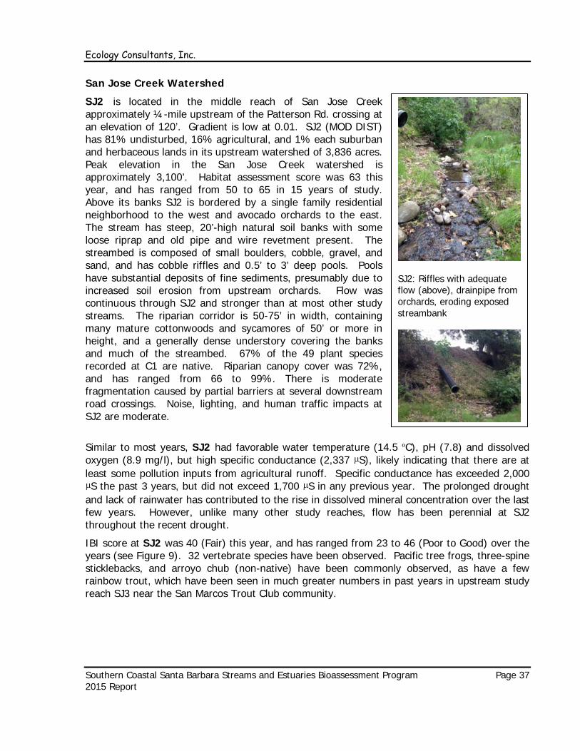
Ecology Consultants, Inc.
Southern Coastal Santa Barbara Streams and Estuaries Bioassessment Program Page 37 2015 Report
San Jose Creek Watershed
SJ2 is located in the middle reach of San Jose Creek approximately ¼-mile upstream of the Patterson Rd. crossing at an elevation of 120’. Gradient is low at 0.01. SJ2 (MOD DIST) has 81% undisturbed, 16% agricultural, and 1% each suburban and herbaceous lands in its upstream watershed of 3,836 acres. Peak elevation in the San Jose Creek watershed is approximately 3,100’. Habitat assessment score was 63 this year, and has ranged from 50 to 65 in 15 years of study. Above its banks SJ2 is bordered by a single family residential neighborhood to the west and avocado orchards to the east. The stream has steep, 20’-high natural soil banks with some loose riprap and old pipe and wire revetment present. The streambed is composed of small boulders, cobble, gravel, and sand, and has cobble riffles and 0.5’ to 3’ deep pools. Pools have substantial deposits of fine sediments, presumably due to increased soil erosion from upstream orchards. Flow was continuous through SJ2 and stronger than at most other study streams. The riparian corridor is 50-75’ in width, containing many mature cottonwoods and sycamores of 50’ or more in height, and a generally dense understory covering the banks and much of the streambed. 67% of the 49 plant species recorded at C1 are native. Riparian canopy cover was 72%, and has ranged from 66 to 99%. There is moderate fragmentation caused by partial barriers at several downstream road crossings. Noise, lighting, and human traffic impacts at SJ2 are moderate.
Similar to most years, SJ2 had favorable water temperature (14.5 ºC), pH (7.8) and dissolved oxygen (8.9 mg/l), but high specific conductance (2,337 µS), likely indicating that there are at least some pollution inputs from agricultural runoff. Specific conductance has exceeded 2,000 µS the past 3 years, but did not exceed 1,700 µS in any previous year. The prolonged drought and lack of rainwater has contributed to the rise in dissolved mineral concentration over the last few years. However, unlike many other study reaches, flow has been perennial at SJ2 throughout the recent drought.
IBI score at SJ2 was 40 (Fair) this year, and has ranged from 23 to 46 (Poor to Good) over the years (see Figure 9). 32 vertebrate species have been observed. Pacific tree frogs, three-spine sticklebacks, and arroyo chub (non-native) have been commonly observed, as have a few rainbow trout, which have been seen in much greater numbers in past years in upstream study reach SJ3 near the San Marcos Trout Club community.
SJ2: Riffles with adequate flow (above), drainpipe from orchards, eroding exposed streambank
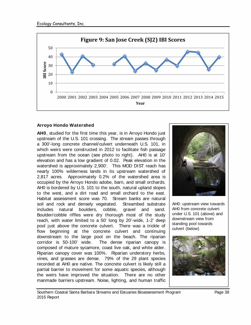
Ecology Consultants, Inc.
Southern Coastal Santa Barbara Streams and Estuaries Bioassessment Program Page 38 2015 Report
Arroyo Hondo Watershed
AH0, studied for the first time this year, is in Arroyo Hondo just upstream of the U.S. 101 crossing. The stream passes through a 300’-long concrete channel/culvert underneath U.S. 101, in which weirs were constructed in 2012 to facilitate fish passage upstream from the ocean (see photo to right). AH0 is at 10’ elevation and has a low gradient of 0.02. Peak elevation in the watershed is approximately 2,900’. This MOD DIST reach has nearly 100% wilderness lands in its upstream watershed of 2,817 acres. Approximately 0.2% of the watershed area is occupied by the Arroyo Hondo adobe, barn, and small orchards. AH0 is bordered by U.S. 101 to the south, natural upland slopes to the west, and a dirt road and small orchard to the east. Habitat assessment score was 70. Stream banks are natural soil and rock and densely vegetated. Streambed substrate includes natural boulders, cobble, gravel and sand. Boulder/cobble riffles were dry thorough most of the study reach, with water limited to a 50’ long by 20’-wide, 1-2’ deep pool just above the concrete culvert. There was a trickle of flow beginning at the concrete culvert and continuing downstream to the large pool on the beach. The riparian corridor is 50-100’ wide. The dense riparian canopy is composed of mature sycamore, coast live oak, and white alder. Riparian canopy cover was 100%. Riparian understory herbs, vines, and grasses are dense. 79% of the 29 plant species recorded at AH0 are native. The concrete culvert is likely still a partial barrier to movement for some aquatic species, although the weirs have improved the situation. There are no other manmade barriers upstream. Noise, lighting, and human traffic
0
10
20
30
40
50
2000 2001 2002 2003 2004 2005 2006 2007 2008 2009 2010 2011 2012 2013 2014 2015
IBI S
core
Year
Figure 9: San Jose Creek (SJ2) IBI Scores
AH0: upstream view towards AH0 from concrete culvert under U.S. 101 (above) and downstream view from standing pool towards culvert (below)

Ecology Consultants, Inc.
Southern Coastal Santa Barbara Streams and Estuaries Bioassessment Program Page 39 2015 Report
impacts to the stream are low/moderate, at AH0 due to the proximity of U.S. 101.
AH1 is located in Arroyo Hondo approximately 1 mile upstream of U.S. 101 at an elevation of 150’. This REF study reach has moderate gradient (0.04) and a watershed area of 2,583 acres that is 100% undisturbed wilderness. A dirt road that extends along the stream about ¼-mile upstream of the study reach is the only human disturbance. Habitat assessment score was 93 this year, had has been between 93 and 95 in 15 years of study. The stream has natural soil and rock banks and natural boulder-dominated streambed with riffles, cascades/falls and plunge pools. The streambed contains clean cobble and gravel deposits ideal for rainbow/steelhead trout spawning, and sand and fine sediment deposits in pools. This year stream flow at AH1 was low but continuous in riffles and cascades, and pools ranged from 1-3’ deep. The riparian canopy at AH1 is dominated by mature sycamore, coast live oak, and white alder. Riparian canopy cover was 99%, and has ranged from 91 to 100%. Riparian understory herbs, vines, and grasses were patchy, as much of the stream banks are made up of large boulders. 81% of the 48 plant species recorded at AH1 are native. Besides the U.S. 101 crossing, there is little habitat fragmentation in Arroyo Hondo, and human traffic impacts to the stream are very low.
AH0, which was limited to standing pools this year, had favorable temperature (16.6 ºC), pH (7.1) and specific conductance (1,092 µS), but very low dissolved oxygen (2.1 mg/l) due to a lack of surface flow and circulation. AH1, which has had perennial flow throughout the recent drought, had optimal water temperature (15.0 ºC), dissolved oxygen (10.3 mg/l), and pH (8.1). Specific conductance (1,126 µS) was favorably low compared to most other study reaches this year, but more than 25% higher compared to any previous year at AH1, indicating that mineral concentrations in the water have become more concentrated due to the drought.
IBI score at AH1 was 55 (Good), and this REF stream has typically scored in the Good or Excellent range in previous years of study (see Figure 10). IBI score at AH0 was 3 (Very Poor). AH0 would be expected to score in the Good to Excellent range when there is sufficient flow and adequate dissolved oxygen. The lack of riffle habitat and extremely low dissolved oxygen levels in residual pools created inhospitable conditions this year for most BMI taxa.
14 vertebrate species were observed at AH0 this year, including red-legged frogs (Rana draytonii) and Pacific tree frogs. 36 vertebrate species have been observed over the years at AH1, including 5 aquatic species. AH1 was the only stream study reach with rainbow trout this year. Other aquatic vertebrates observed at AH1 over the years include southwestern pond turtle, two-striped garter snake (Thamnophis hammondii), Pacific tree frog, and California tree frog.
AH1: cool clean water, ideal substrate for trout spawning.

Ecology Consultants, Inc.
Southern Coastal Santa Barbara Streams and Estuaries Bioassessment Program Page 40 2015 Report
Gaviota Creek Watershed
GAV1 is located in lower Gaviota Creek just upstream of the crossing of the entrance road into Gaviota State Beach at an elevation of 15’. Gradient is low at 0.01. GAV1 (MOD DIST) has 59% undisturbed 40% grazed herbaceous and 1% urban (i.e., roads) lands in its upstream watershed of 12,791 acres. Peak elevation in the watershed is approximately 2,700’. Habitat assessment score was 80 this year, and has ranged from 68 to 85 in 12 years of study. The stream has low, gradually sloped sandy soil banks and a wide floodplain with a thick willow-dominated riparian forest that also includes coast live oaks, sycamores, black cottonwoods, and dense understory plants. Due to a lack of scouring flows the past few years, riparian vegetation has become thick in the streambed, as evidenced by 94% riparian canopy cover this year. This parameter had ranged from 0-80% in previous years. 65% of the 60 plant species recorded at GAV1 are native. The streambed at GAV1 has gentle cobble-dominated riffles and 0.5’ to 3.0’ deep pools underlain mostly by sand and fine sediments. Flow was reduced to a trickle in riffles at the time of the spring survey this year, as it has been in the past few years. The downstream access road crossing and several upstream crossings by U.S. 101 create grade changes that inhibit movement by most fish and other aquatic species, thus partially fragmenting the aquatic habitat. Noise, lighting, and human traffic impacts at GAV1 from U.S. 101 and Gaviota State Beach are moderate.
LC1 (MOD DIST) is located in Las Canovas Creek just upstream of its confluence with Gaviota Creek at an elevation of 320’. This site is high gradient (0.06) and drains an upstream watershed of 1,024 acres that is comprised of 89% undisturbed wilderness, 11% herbaceous lands, and less than 0.5% urbanized lands including a paved road and several rural residential structures. Peak elevation in the watershed is approximately 2,700’. LC1 is abutted by the paved road above its northern bank, and wilderness to the south. Habitat assessment score
GAV1: thick riparian canopy with watercress filling much of streambed
0
20
40
60
80IB
I Sco
re
Year
Table 10: Arroyo Hondo Watershed IBI Scores
AH0
AH1

Ecology Consultants, Inc.
Southern Coastal Santa Barbara Streams and Estuaries Bioassessment Program Page 41 2015 Report
was 73. The stream has steep rock and soil banks that are actively eroding. The northern bank has been fortified in sections with loose boulders in an effort to protect the access road. The boulder-dominated streambed has alternating falls/cascades and pools of 1’ to 3’ deep. Flow was low but continuous throughout LC1. Fine sediments largely embed underlying cobble and gravel deposits in much of the streambed, particularly in pools. Mature alders, sycamores, and coast live oaks form a dense riparian canopy (94% cover), with dense understory plants. 74% of the 23 plant species recorded at LC1 are native. The culvert connecting Las Canovas Creek to Gaviota Creek under U.S. 101 creates a grade drop that likely inhibits movement of most fish and other aquatic species. Noise, lighting, and human traffic impacts at LC1 are light.
GAV1 had low stream temperature (15.1 ºC), optimal dissolved oxygen (7.3 mg/l), normal pH (7.7), and elevated conductivity (2,518 µS), as has been the case for the last several years. Comparatively, tributary LC1 had lower temperature (14.3 ºC), higher dissolved oxygen (10.4 mg/l) and pH (8.2), and much lower conductivity (838 µS).
IBI score was 11 (Poor) at GAV1 this year, its lowest score in 12 years of study, and slightly worse than last year (14, Poor) (see Figure 11). The past two years, GAV1 has had low insect/EPT richness and representation by other sensitive taxa, predators, and shredders, and a high proportion of tolerant taxa including chironomids and non-insects, which made up about 80% of the sample this year and 70% last year. IBI scores have varied widely at GAV1 over the years, having been as high as 54 in 2013, and reaching the Good category several times. As with many other streams, the drought appears to have limited the BMI community at GAV1 the past two years, it dried to the point of having standing pools only, and presumably low dissolved oxygen levels, in September 2013 and 2014. LC1 had an IBI score of 43 (Fair), having high EPT and insect family richness, fair representation by other sensitive taxa and shredders+predators, and fairly high proportion of tolerant taxa, particularly gastropods and chironomids. This site has continued to have perennial flow despite the recent drought, as observed in September 2014 and 2015.
36 vertebrate species have been observed at GAV1 over the years, including 5 aquatic species: three-spine sticklebacks, arroyo chubs, southwestern pond turtles, western toads, and Pacific tree frogs. 13 vertebrate species were observed at LC1 this year, including California newts and Pacific tree frogs.
0102030405060
2002 2003 2004 2005 2006 2007 2008 2009 2010 2011 2012 2013 2014 2015
IBI S
core
Year
Figure 11: Gaviota Creek Watershed IBI Scores
GAV1
LC1

Ecology Consultants, Inc.
Southern Coastal Santa Barbara Streams and Estuaries Bioassessment Program Page 42 2015 Report
2. Drought Effects
Table A-5 in the Appendix summarizes the results of the ANOVAs comparing IBI scores by disturbance group (REF, MOD DIST, and HIGH DIST) for the 3 flow groups:
1. (F-F): Flow in spring and Flow previous fall 2. (F-P): Flow in spring, Pools only or dry previous fall 3. (P-P): Pools in spring, Pools only or dry previous fall
There were not discernable differences in IBI score among flow groups at HIGH DIST sites, as apparently the high level of human disturbance impacts masked any effects from the drought. For REF sites, mean IBI score was significantly higher for the F-F group (51) compared to F-P (22) and P-P (4) groups (p=0.0006, r2= 0.77). Results for MOD DIST sites were similar (mean IBI score 44 for F-F group, 18 for F-P group, 3 for P-P group, <0.0001, r2= 0.74). We combined the REF and MOD DIST groups to improve statistical power (i.e., due to a greater number of samples). Differences in mean IBI score were highly significant between the F-F (47), F-P (19), and P-P (4) groups (p<0.0001, r2= 0.74). Figure 12 illustrates the results for the HIGH DIST and REF+MOD DIST groups.
All 7 BMI core metrics had far better values for F-F compared to F-P and P-P groups for the REF+MOD DIST groups, all with high levels of significance (p range <0.0001 to 0.0005, r2 range 0.42 to 0.64) (see Table A-5). The results with respect to IBI scores and core metrics show that where stream flow is intermittent the aquatic community is stressed due to loss of riffle habitat, stagnation of residual pools and low dissolved oxygen levels, or complete drying. In such conditions, many aquatic inhabitants become limited or disappear including vertebrates such as steelhead/rainbow trout and other fish, and many sensitive BMIs including Caenidae, Lepidostomatidae, Glossostomatidae, Rhyacophilidae, and Elmidae, all of which had significantly (p<0.05) or near-significantly (0.05<p≤0.10) higher abundances for the F-F group compared to F-P and P-P groups for REF+MOD DIST sites (see Table A-5). What persists in these stressed conditions or rapidly recolonizes when flow returns are some amphibians (e.g., tree frogs) and tolerant BMIs including Chironomidae, Dytisidae, and Simulidae, all of which had significantly or near significantly higher abundances in the F-P group compared to the F-F group. Interestingly, mean BMI density was not different between flow groups for REF+MOD DIST sites (p=0.32, r2= 0.08).
3. Year-to-Year Trends in IBI Scores
The results of the ANOVA of IBI score year to year for the REF group (n=66) are summarized in Table A-6. Figure 13 illustrates the ANOVA. Using only REF sites eliminated any potentially confounding influences of human disturbance on IBI scores, allowing the relationship between IBI scores and rainfall to be more clearly examined.
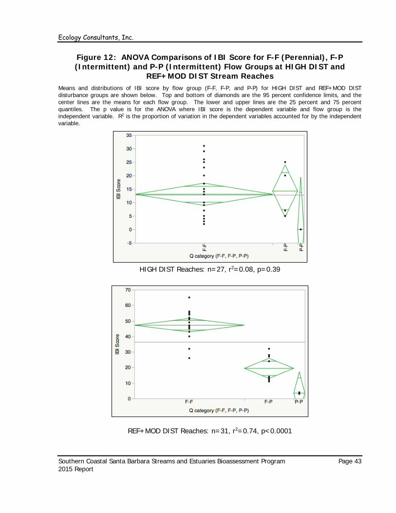
Ecology Consultants, Inc.
Southern Coastal Santa Barbara Streams and Estuaries Bioassessment Program Page 43 2015 Report
Figure 12: ANOVA Comparisons of IBI Score for F-F (Perennial), F-P (Intermittent) and P-P (Intermittent) Flow Groups at HIGH DIST and
REF+MOD DIST Stream Reaches Means and distributions of IBI score by flow group (F-F, F-P, and P-P) for HIGH DIST and REF+MOD DIST disturbance groups are shown below. Top and bottom of diamonds are the 95 percent confidence limits, and the center lines are the means for each flow group. The lower and upper lines are the 25 percent and 75 percent quantiles. The p value is for the ANOVA where IBI score is the dependent variable and flow group is the independent variable. R2 is the proportion of variation in the dependent variables accounted for by the independent variable.
HIGH DIST Reaches: n=27, r2=0.08, p=0.39
REF+MOD DIST Reaches: n=31, r2=0.74, p<0.0001

Ecology Consultants, Inc.
Southern Coastal Santa Barbara Streams and Estuaries Bioassessment Program Page 44 2015 Report
Figure 13: ANOVA Comparisons of IBI Score for REF Study Reaches by Year
Means and distributions of IBI score for REF study reaches by year are shown below. Top and bottom of diamonds are the 95 percent confidence limits, and the center lines are the means for each dis group. The lower and upper lines are the 25 percent and 75 percent quantiles. The p value is for the ANOVA where IBI score is the dependent variable and year is the independent variable. R2 is the proportion of variation in the dependent variables accounted for by the independent variable. (p<0.0001, r2 = 0.59, n=66).

Ecology Consultants, Inc.
Southern Coastal Santa Barbara Streams and Estuaries Bioassessment Program Page 45 2015 Report
The REF group had significantly lower IBI scores for three years compared to most of the other years:
1. 2005, which had a mean IBI score of 37 and was the second highest rainfall year in over 130 years of records, and:
2. 2014, which had a mean IBI score of 33, and was the 3rd consecutive year of severe drought, and one of the lowest rainfall years on record.
3. 2015, which had a mean IBI score of 24, and was the 4th consecutive year of severe drought, and one of the lowest rainfall years on record.
There were not any other significant differences in mean IBI score among years for the REF streams. The remaining years had average IBI scores ranging from 47 to 63. Based on the above, IBI scores appear to be naturally lower immediately following extremely high rainfall years, and after periods of prolonged drought, compared to more moderate rainfall years. This makes sense, as:
• Extremely high rainfall years produce high stream discharges that scour and wash out large quantities of streambed material and BMIs in some sections, and bury them in others. The following spring, the BMI community is in a state of recovery, as evidenced by lower overall BMI density, lower relative abundances of many taxa such as pool dwelling Caenidae and Leptohyphidae, Ostracoda, and Gastropoda, and higher relative abundances of early colonizers including Baetidae and Simulidae.
• Periods of prolonged drought (i.e., 2011 to 2015) can result in the loss of surface flow in normally perennial streams. When surface flow ceases, aquatic habitat becomes greatly reduced (i.e., standing pools with dissolved oxygen crashes) or is completely lost (dry), and relatively few aquatic taxa can survive. The aquatic community begins to recover when stream flows return via colonization from remaining wet reaches of the stream or other watersheds (e.g., by aerial insects). This state of recovery is typically reflected by lower BMI community integrity (and lower IBI scores) when surveys are completed the following spring.
• More normal rainfall years typically create more stable and sustained flows, which create the conditions for a more balanced and mature BMI community, and more stable, higher IBI scores.
The ANOVAs comparing IBI score by disturbance group for each year summarized in Table A-7, and Figure 14 illustrates the ANOVAs for select years (2012 and 2015). From 2000 to 2014, there were significant differences amongst the disturbance groups in mean IBI score, which increased appropriately from HIGH DIST to MOD DIST to REF every year. This includes 2005, the extreme high rainfall year, and 2014, which followed three consecutive years of drought. MOD DIST and REF scores were depressed in 2005 and 2014, but the IBI still differentiated appropriately between each disturbance group. This year (2015) was the first time that there were not any significant differences in mean IBI score between disturbance groups. The prolonged drought caused intermittent flow conditions in 2014 and 2015 at 2 of the 3 REF study reaches, M4 (IBI score 4, Very Poor) and C3 (IBI score 14, Poor). These study reaches have typically scored in the Good to Excellent range in years of perennial flow. AH1 was the only REF study reach with year-round flow the past two years, and had an IBI score of 55 (Good).

Ecology Consultants, Inc.
Southern Coastal Santa Barbara Streams and Estuaries Bioassessment Program Page 46 2015 Report
Figure 14: ANOVAs of IBI Score for HIGH DIST, MOD DIST, and REF Disturbance Groups for Selected Years
Means and distributions of IBI score for each of the three disturbance groups for selected years (2012 and 2015) are shown below. Top and bottom of diamonds are the 95 percent confidence
limits, and the center lines are the means. The lower and upper lines are the 25 percent and 75 percent quantiles.
2012 (p<0.0001, r2 =
0.85, n=14)
2015 (p=0.2497, r2 =
0.19, n=16)

Ecology Consultants, Inc.
Southern Coastal Santa Barbara Streams and Estuaries Bioassessment Program Page 47 2015 Report
C. Estuaries
The following discusses the physiochemical attributes and BMI communities of each individual estuary and their respective watersheds. Photographs are also provided. See Table A-4 for a summary of data collected at the study estuaries.
1. Study Estuaries
Carpinteria Creek Estuary
The Carpinteria Creek estuary (MOD DIST) has an upstream watershed of approximately 9,600 acres, including approximately 80% wilderness, 17% agriculture, and 3% urban development. The estuary is approximately 800’ long by 20-100’ wide, and had a maximum depth of 2.5’ feet deep in the center, as compared to 4’ deep last year. The width, depth, and overall volume of water were noticeably lower this year, as was the case in all the study estuaries due to the drought. The estuary was closed from the ocean by an approximately 150’ wide sand berm. Tide conditions were high at the time of the survey. Bottom substrate was mostly sand. There was a thin surface layer of fine sediment and organic detritus along most of the bottom area, with scattered clumps of submerged algae and organic litter. There are sand dunes along the southern boundary of the estuary, and fringing vegetation ranged from 10-60’ in width and was composed of approximately 80% natives including cattails, pickleweed, and salt grass, and 20% non-natives including iceplant and ornamental shrubs. The estuary is abutted to the east and west by campgrounds of Carpintera State Beach, and is bisected by a bridge. There is heavy human traffic in this area from the adjacent campsites, bridge, and State beach. Habitat assessment score was 53/100.
Water chemistry measurements were taken at the surface and at 1.5’ depth near the downstream end of the estuary. Water surface temperature was 23.4 ºC, salinity was 1.5 ppt, dissolved oxygen was low at 3.6 mg/l, and pH was 7.8. Near the bottom temperature was 23.0 ºC, salinity was 1.4 ppt, and dissolved oxygen was 3.5 mg/l. Like last year, the water column was well mixed, but surprisingly salinity was lower compared to last year (5.2 ppt), as was dissolved oxygen (6.5 mg/l last year).
A total of 7 different BMI taxa were observed at the Carpinteria Creek estuary this fall, and BMI density was high at 2,143/m2, as compared to 9 taxa and 3,000/ m2 last year. Chironomidae
Carpinteria Creek estuary: wide beach berm and lower water level compared to previous years.

Ecology Consultants, Inc.
Southern Coastal Santa Barbara Streams and Estuaries Bioassessment Program Page 48 2015 Report
was the most abundant taxa, and Oligochaeta, Cladocera, Gastropoda, and Baetidae were found in significant numbers. These taxa were all found in significant numbers last year.
Sycamore Creek Estuary
Sycamore Creek estuary (HIGH DIST) has an upstream watershed of approximately 2,600 acres, including approximately 43% wilderness, 55% urban development, and 2% agriculture (mainly orchards). Upstream of Cabrillo Blvd., the estuary is a channelized extension of Sycamore Creek, and approximately 25-30’ wide and 1-2’ deep in the center. This section was not surveyed due to access problems. Downstream of Cabrillo Blvd. the estuary stretched along the beach for approximately 30’ long and 10-20’ wide at the time of the field survey on September 23. The estuary was closed to the ocean by a natural sand berm of approximately 150’ wide. Tide conditions were low at the time of the survey (11 AM). The estuary was smaller and shallower (1.5’ maximum depth) compared to previous years. Bottom substrate was mostly sand. There was a thin surface layer of fine sediment and organic detritus along most of the bottom area, and scattered clumps of submerged algae, submerged grass, and organic litter. Fringing vegetation ranged from 0-10’ wide around the estuary, and was composed of approximately 20% native and 80% non-native cover. There is heavy human traffic in this area from the adjacent roadways, boardwalk, and beach. Habitat assessment score was 20/100.
Water surface temperature was 25.7 ºC, salinity was high at 9.1 ppt, dissolved oxygen was 14.6 mg/l, and pH was 8.6. Near the bottom temperature was 24.4 ºC and salinity was 9.1 ppt. Overall, the water column was well mixed, and salinity was about half of last year (19.1 ppt).
This fall, a total of 7 BMI taxa were observed and BMI density was 3,000/ m2, compared to 6 taxa and 1,579/ m2 last year. The most abundant taxa this year were Corixidae, Ostracoda, and Chironomidae, also with some Oligochaeta and Polychaeta. BMI composition was similar last year.
Above: Estuary perimeter reduced due to drought, vegetation growing in previously inundated area (mid-right). Below: Submerged grass bed in remaining estuary at Cabrillo Blvd. bridge.

Ecology Consultants, Inc.
Southern Coastal Santa Barbara Streams and Estuaries Bioassessment Program Page 49 2015 Report
Mission Creek Estuary
The Mission Creek estuary (HIGH DIST) has an upstream watershed of approximately 6,900 acres, including approximately 48% wilderness, 50% urban development, and 2% agriculture (mainly orchards). Upstream of Cabrillo Blvd., the estuary is a channelized extension of Mission Creek, and approximately 40 feet wide and 4 to 5 feet deep in the center. This section was not surveyed due to access problems. Downstream of Cabrillo Blvd. the estuary stretched along the beach for approximately 600’ in length and 30-80’ wide on September 23. The estuary did not connect with the Laguna Channel to the east as it has in previous years. The estuary was closed from the ocean by an approximately 100’ wide sand berm at mid-tide. Maximum water depth was 3’, and bottom substrate was mostly sand. There was a thin surface layer of fine sediment and organic detritus along most of the bottom area, and scattered clumps of submerged algae and grass and organic material. Sand dunes along the northern boundary of the estuary are sparsely vegetated with ice plant and a few native shrubs and herbs. Fringing marsh vegetation including cattails, pickleweed and non-native grasses were more prominent and wider (up to 20’) along the western and eastern edges compared to previous years. Overall, vegetation was approximately 40% native and 60% non-native in overall cover. There is heavy human traffic in this area from the adjacent roadways, boardwalk, Stern’s Wharf and the beach. Habitat assessment score was 40/100.
Water chemistry and BMI sampling was conducted along the southern margin end nearest the ocean. Water chemistry was fairly uniform with depth, with temperatures of 27.1-26.2 ºC, salinity of 3.0-3.1 ppt, dissolved oxygen of 14.0 mg/l, and pH of 7.5.
6 BMI taxa were observed at the Mission Creek estuary this fall, and BMI density was low at 288/m2, as compared with 10 BMI taxa and BMI density of 1,765/m2 last year. Ostracoda comprised about half of the BMIs collected this year, and Chironomidae, Amphipoda (Gammaridae), and Baetidae were also present.
Above: westerly view across the estuary. Below: northerly view across the estuary, notice marsh vegetation establishing along northern fringe.

Ecology Consultants, Inc.
Southern Coastal Santa Barbara Streams and Estuaries Bioassessment Program Page 50 2015 Report
Arroyo Burro Estuary
Arroyo Burro estuary (HIGH DIST) has an upstream watershed of approximately 6,800 acres, including approximately 49% wilderness, 4% herbaceous open space, 7% agriculture (mainly orchards), and 40% urban development. The upstream inlet to the estuary is just below the Cliff Drive bridge. The estuary was approximately 1,500’ long, 30-50’ wide, and up to 4’ deep at the time of the September 23 survey. For the majority of its length, this estuary is bordered by natural scrub vegetation and cliffs to the east, and Hendry’s beach and parking area to the west. The northern upstream portion of the estuary is surrounded by thick, mostly native marsh and riparian forest of 25-100’ in width that was enhanced by a major habitat restoration project undertaken by the City. The estuary was closed to the ocean by a 50’-wide beach berm at the time of the September 23 survey during mid-tide conditions. Bottom substrate was composed mostly of sand, with a thin layer of fine sediments and detritus and scattered algae and organic material. Some cobble and gravel was present nearest the upstream end. Noise, lighting and human traffic impacts are high. Habitat assessment score was 50/100.
Water chemistry and BMI sampling was conducted at the downstream estuary margin. Unlike past years, there was no stratification of water chemistry readings with depth. Water temperature was 25.5-26.0 ºC, salinity 6.2-6.3 ppt, dissolved oxygen 12.9 mg/l, and pH 8.3.
Oddly, only 2 BMIs (both Chironomidae) were found in the samples collected at the Arroyo Burro estuary this year. BMI density has typically ranged from 800-2,500/m2 in past years, and 5-10 different BMI taxa have been found. 50 to 100 6-8” long Striped Mullet (Mugil cephalus) were observed schooling in the lower estuary, and bird activity was heavy as usual in and around the estuary.
Northerly view from downstream end of the estuary. Mouth closed to ocean, which is unusual for this site.

Ecology Consultants, Inc.
Southern Coastal Santa Barbara Streams and Estuaries Bioassessment Program Page 51 2015 Report
Goleta Slough Estuary
The Goleta Slough estuary (HIGH DIST) has the largest watershed area of all study estuaries at 30,400 acres, and receives runoff from several major tributary streams including Tecolotito Creek, San Jose Creek, San Pedro Creek, Maria Ygnacio Creek, and Atascadero Creek. The watershed consists of 53% wilderness, 25% agriculture, 20% urban, and 2% herbaceous undeveloped lands. The 430-acre Goleta Slough wetlands include the approximately 1,200’ long, 100-300’ wide estuary along Goleta Beach, upstream creek and tidal channels, salt marsh, salt flats and freshwater marsh. The estuary was up to 5’ deep and closed to the ocean by a 100’ wide sand berm at the time of the September 23 survey during high tide conditions. The estuary is bordered by 100’ high cliffs and natural scrub and wetland vegetation to the north and Goleta Beach including the Beachside restaurant and pier parking area to the south. The southern banks are armored with riprap to protect the parking area, and vegetation in this area is sparse and composed mostly of ornamental shrubs. The estuary bottom substrate was composed mostly of sand, with a thin layer of fine sediments and detritus and scattered algae and organic material. Noise, lighting and human traffic impacts are high. Habitat assessment score was 53/100.
Water chemistry and BMI sampling was conducted at the southern, downstream estuary margin. Water chemistry readings were uniform with depth, with very high water temperature (31.0-31.2 ºC) and dissolved oxygen (22.5 mg/l), high salinity (21.6-21.9 ppt), and pH of 8.3. Last year salinity was extremely high at over 43 ppt, dissolved oxygen was very low at 2.5 mg/l, and water temperature was lower at 22.8 ºC.
This fall, 3 BMI taxa, Amphipoda (Corophiidae), Ostracoda, and Polychaeta were observed in significant numbers, and BMI density was 417/ m2 in Goleta Slough, compared to 4 taxa and 1,923/ m2 last year. BMI composition was similar last year, but Corixidae were also present.
Goleta Slough: greater surface area and depth make drought effects less noticeable than many smaller sites. Extensive algae beds (below).

Ecology Consultants, Inc.
Southern Coastal Santa Barbara Streams and Estuaries Bioassessment Program Page 52 2015 Report
Tecolote Creek Estuary
Tecolote Creek estuary (MOD DIST) has an upstream watershed of approximately 3,700 acres, with land cover of approximately 75% wilderness, 2% herbaceous, 19% agriculture (mainly orchards), and 4% urban development. The estuary is long and narrow, extending north to south approximately 500 feet in length, with a width of 20 to 40 feet. The estuary was closed from the ocean by an approximately 50 feet wide sand berm at the time of the September 18 survey during mid tide conditions. Water levels were noticeably lower (2’ maximum depth) than previous years due to the drought. Bottom substrate was mostly sand, with some gravel and cobble near the mouth. There was a thin surface layer of fine sediment and organic detritus and scattered clumps of submerged algae, grass, and organic litter. The area surrounding the estuary has been restored and preserved as a natural habitat area, which was presumably a condition of developing the Baccara Resort to the west. Thick riparian scrub and coastal scrub habitat with approximately 90 percent native cover and a width of about 300 feet borders both west and east sides of the estuary. Unpaved trails extend through the habitat area to the beach and a clubhouse that is part of the Baccara Resort. A footbridge crosses the estuary at its upstream end. Overall, human traffic and noise are light to moderate. Habitat assessment score was 75/100.
Water and BMI sampling was completed at the downstream end of the estuary. Water chemistry readings were uniform with depth, with water temperature of 24.1-24.5 ºC, dissolved oxygen of 11.2 mg/l, salinity of 2.0 ppt and pH of 8.2.
This year 10 BMI taxa were observed at the estuary, and BMI density was 229/m2, compared to 5 BMI taxa and 79/m2 last year. The most abundant taxa were Ostracoda and Chironomidae, while Gammaridae, Coenagrionidae, Hydrophilidae, Dolichopodidae and Gastropoda were also found in significant numbers.
Tecolote Estuary: water level lower than previous years (2’ max. depth), surrounded by thick cattail/tule beds.

Ecology Consultants, Inc.
Southern Coastal Santa Barbara Streams and Estuaries Bioassessment Program Page 53 2015 Report
Bell Canyon Estuary
Bell Canyon estuary (MOD DIST) has an upstream watershed of approximately 3,900 acres, with land cover of approximately 75% wilderness, 6% herbaceous, 14% agriculture (mainly orchards), and 5% urban development. Bell Canyon estuary is about ¼-mile east of the Tecolote estuary, both having very similar watershed size and land use patterns. Bell Canyon estuary was closed from the ocean by an approximately 100 feet wide sand berm at the time of the September 18 survey during mid tide conditions. Water levels were very low with approximately 200’ length, 10-20’ width, and only 0.5’ maximum depth. Bottom substrate was mostly sand with a thin surface layer of fine sediment and organic detritus and scattered clumps of submerged algae and organic litter. The estuary is bordered by natural areas immediately to the west and north, the Sandpiper Golf Course to the east, and an oil and gas plant is situated further north. Fringing vegetation is approximately 60% native (e.g., tule beds, riparian scrub) and 40% non-native (e.g., ornamental trees and shrubs). Human traffic and noise are moderate. Habitat assessment score was 70/100.
Water and BMI sampling was completed at the downstream end of the estuary. Water chemistry readings were uniform with depth, with very high water temperature (30.4 ºC) and dissolved oxygen (15.1 mg/l), pH of 8.2, and salinity of 4.1 ppt and pH of 8.2. Salinity was very high last year at 31.5 ppt.
This year 6 BMI taxa were observed at Bell Canyon estuary, and BMI density was 556/m2, compared to 4 BMI taxa and 3,000/m2 last year. The most abundant taxa this year was Ostracoda, which made up almost 80% of the BMIs sampled. BMI composition was very similar last year, which is interesting given the dramatic drop in salinity.
Bell Estuary: Surface area greatly reduced, maximum depth less than 1’ due to drought. Area shown in bottom photo was completely inundated last year.
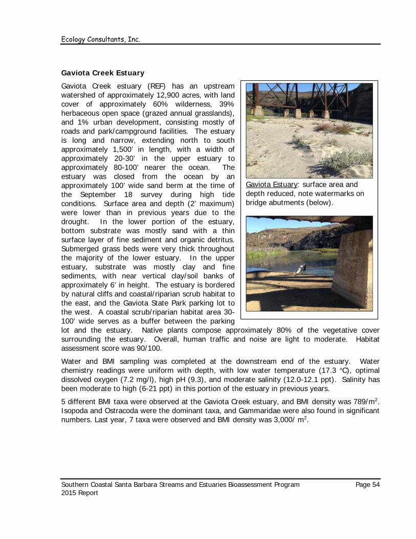
Ecology Consultants, Inc.
Southern Coastal Santa Barbara Streams and Estuaries Bioassessment Program Page 54 2015 Report
Gaviota Creek Estuary
Gaviota Creek estuary (REF) has an upstream watershed of approximately 12,900 acres, with land cover of approximately 60% wilderness, 39% herbaceous open space (grazed annual grasslands), and 1% urban development, consisting mostly of roads and park/campground facilities. The estuary is long and narrow, extending north to south approximately 1,500’ in length, with a width of approximately 20-30’ in the upper estuary to approximately 80-100’ nearer the ocean. The estuary was closed from the ocean by an approximately 100’ wide sand berm at the time of the September 18 survey during high tide conditions. Surface area and depth (2’ maximum) were lower than in previous years due to the drought. In the lower portion of the estuary, bottom substrate was mostly sand with a thin surface layer of fine sediment and organic detritus. Submerged grass beds were very thick throughout the majority of the lower estuary. In the upper estuary, substrate was mostly clay and fine sediments, with near vertical clay/soil banks of approximately 6’ in height. The estuary is bordered by natural cliffs and coastal/riparian scrub habitat to the east, and the Gaviota State Park parking lot to the west. A coastal scrub/riparian habitat area 30-100’ wide serves as a buffer between the parking lot and the estuary. Native plants compose approximately 80% of the vegetative cover surrounding the estuary. Overall, human traffic and noise are light to moderate. Habitat assessment score was 90/100.
Water and BMI sampling was completed at the downstream end of the estuary. Water chemistry readings were uniform with depth, with low water temperature (17.3 ºC), optimal dissolved oxygen (7.2 mg/l), high pH (9.3), and moderate salinity (12.0-12.1 ppt). Salinity has been moderate to high (6-21 ppt) in this portion of the estuary in previous years.
5 different BMI taxa were observed at the Gaviota Creek estuary, and BMI density was 789/m2. Isopoda and Ostracoda were the dominant taxa, and Gammaridae were also found in significant numbers. Last year, 7 taxa were observed and BMI density was 3,000/ m2.
Gaviota Estuary: surface area and depth reduced, note watermarks on bridge abutments (below).
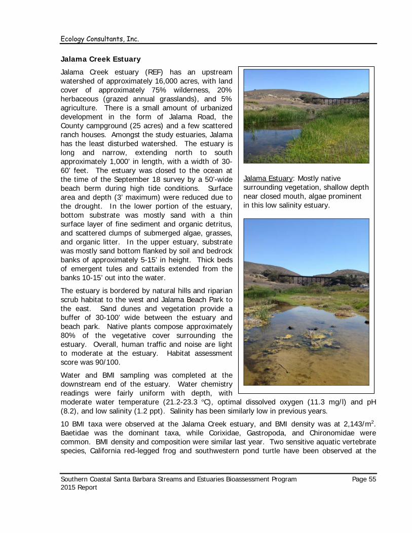
Ecology Consultants, Inc.
Southern Coastal Santa Barbara Streams and Estuaries Bioassessment Program Page 55 2015 Report
Jalama Creek Estuary
Jalama Creek estuary (REF) has an upstream watershed of approximately 16,000 acres, with land cover of approximately 75% wilderness, 20% herbaceous (grazed annual grasslands), and 5% agriculture. There is a small amount of urbanized development in the form of Jalama Road, the County campground (25 acres) and a few scattered ranch houses. Amongst the study estuaries, Jalama has the least disturbed watershed. The estuary is long and narrow, extending north to south approximately 1,000’ in length, with a width of 30-60’ feet. The estuary was closed to the ocean at the time of the September 18 survey by a 50’-wide beach berm during high tide conditions. Surface area and depth (3’ maximum) were reduced due to the drought. In the lower portion of the estuary, bottom substrate was mostly sand with a thin surface layer of fine sediment and organic detritus, and scattered clumps of submerged algae, grasses, and organic litter. In the upper estuary, substrate was mostly sand bottom flanked by soil and bedrock banks of approximately 5-15’ in height. Thick beds of emergent tules and cattails extended from the banks 10-15’ out into the water.
The estuary is bordered by natural hills and riparian scrub habitat to the west and Jalama Beach Park to the east. Sand dunes and vegetation provide a buffer of 30-100’ wide between the estuary and beach park. Native plants compose approximately 80% of the vegetative cover surrounding the estuary. Overall, human traffic and noise are light to moderate at the estuary. Habitat assessment score was 90/100.
Water and BMI sampling was completed at the downstream end of the estuary. Water chemistry readings were fairly uniform with depth, with moderate water temperature (21.2-23.3 ºC), optimal dissolved oxygen (11.3 mg/l) and pH (8.2), and low salinity (1.2 ppt). Salinity has been similarly low in previous years.
10 BMI taxa were observed at the Jalama Creek estuary, and BMI density was at 2,143/m2. Baetidae was the dominant taxa, while Corixidae, Gastropoda, and Chironomidae were common. BMI density and composition were similar last year. Two sensitive aquatic vertebrate species, California red-legged frog and southwestern pond turtle have been observed at the
Jalama Estuary: Mostly native surrounding vegetation, shallow depth near closed mouth, algae prominent in this low salinity estuary.

Ecology Consultants, Inc.
Southern Coastal Santa Barbara Streams and Estuaries Bioassessment Program Page 56 2015 Report
Jalama estuary during the bioassessment surveys. Sensitive aquatic vertebrates have not been observed at any of the other study estuaries.
2. Estuary BMI Indicator Taxa and Metrics
BMI Taxa
Results of the ANOVAs of individual BMI taxa by disturbance group are summarized in Table A-8. Figure 15 illustrates ANOVAs for selected taxa. Sensitive taxa, or those with significantly higher mean abundance at REF sites compared to HIGH DIST sites, were Isopoda (p=0.0001, r2 = 0.37), Gammaridae (p=0.0013, r2 = 0.29), Mystidacea (p=0.0072, r2 = 0.22), Baetidae (p=0.19, r2 = 0.01), and Acari (p=0.02, r2 = 0.18). Aeshnidae (p=0.14, r2 = 0.10) also had higher mean abundance at REF sites compared to HIGH DIST sites, although not with significant results (i.e., p>0.05).
Taxa with higher mean abundance at HIGH DIST sites compared to REF sites include Corixidae (p=0.17, r2 = 0.09), Ostracoda (p=0.22, r2 = 0.07), Oligochaeta (p=0.46, r2 = 0.04), Dytisidae (p=0.58, r2 = 0.03), Cladocera (p=0.70, r2 = 0.02), Ephydridae (p=0.70, r2 = 0.02), and Bivalvia (zebra mussel) (p=0.62, r2 = 0.02). The statistical test results for these “tolerant” taxa are not nearly as strong as those for the sensitive taxa. The spotty distribution of many of the tolerant taxa in many cases contributed to relatively low r2 and high p.
Chironomidae had significantly highest mean abundance at MOD DIST sites (p=0.01, r2 = 0.21), as did Coenagrionidae (p=0.04, r2 = 0.15). Ceratopogonidae (p=0.06, r2 = 0.13) and Hydrophilidae (p=0.19, r2 = 0.08) also had highest mean abundance at MOD DIST sites, although not at a significant level. Gastropoda abundance was higher at REF and HIGH DIST sites and lowest at MOD DIST (p=0.38, r2 = 0.05), and Polychaeta (p=0.29, r2 = 0.06) showed the same pattern. Copepoda (p=0.79, r2 = 0.01) had similar mean abundance for all three disturbance groups. All of these taxa can be considered to have moderate disturbance tolerance. No tolerance sensitivity was assigned to Corophiidae, as it has only been observed at very high salinity sites, all of which have been HIGH DIST thus far.
BMI Metrics
Results of the BMI metric ANOVAs by disturbance group are summarized in Table A-9. The 6 taxa identified above as being sensitive to human disturbance (Isopoda, Gammaridae, Mystidacea, Acari, Baetidae, and Aeshnidae) were combined into % sens BMIs. The 7 taxa identified above as being tolerant of disturbance (Ostracoda, Corixidae, Oligochaeta, Dytisidae, Cladocera, Ephydridae, and zebra mussel) were combined into % tol BMIs. Figure 16 illustrates ANOVAs for % sens BMIs and % tol BMIs.
% sens BMIs is the best indicator metric thus far. It decreases in mean value from REF to MOD DIST to HIGH DIST, with the REF mean being significantly higher compared to MOD DIST and HIGH DIST means with impressive p (<0.0001) and r2 (0.74). % tol BMIs trends in the opposite fashion, decreasing in mean value from HIGH DIST to MOD DIST to REF, with the HIGH DIST mean being significantly higher than the REF mean, but with less impressive p (0.0005) and r2 (0.32).

Ecology Consultants, Inc.
Southern Coastal Santa Barbara Streams and Estuaries Bioassessment Program Page 57 2015 Report
Figure 15: ANOVAs of Mean Abundance of Selected BMI Taxa in Estuaries for REF, MOD DIST, and HIGH DIST Groups
Baetidae and Corixidae abundance for each of the three disturbance groups are shown below. Top and bottom of diamonds are the 95 percent confidence limits, and the center lines are the means. The lower and upper lines are the 25 percent and 75 percent quantiles. N=42.
Corixidae p=0.17
r2 = 0.09
High Disturbance Tolerance
Baetidae p=0.01
r2 = 0.19
Low Disturbance Tolerance

Ecology Consultants, Inc.
Southern Coastal Santa Barbara Streams and Estuaries Bioassessment Program Page 58 2015 Report
Figure 16: ANOVAs of % Sensitive BMIs and % Tolerant BMIs in Estuaries for REF, MOD DIST, and HIGH DIST Groups
% sensitive BMIs and % tolerant BMIs for each of the three disturbance groups are shown
below. Top and bottom of diamonds are the 95 percent confidence limits, and the center lines are the means. The lower and upper lines are the 25 percent and 75 percent quantiles. N=42
P<0.0001 r2 = 0.76
P=0.0005 r2 = 0.32

Ecology Consultants, Inc.
Southern Coastal Santa Barbara Streams and Estuaries Bioassessment Program Page 59 2015 Report
%cg, 100+(%cg-%pred), and # taxa decrease in mean value along a disturbance gradient, while % pred, % dominant taxa, and % two dominant taxa increase. However, r2 is relatively low (0.08-0.16) for these metrics, and %cg is the only one that had a statistically significant difference in means. # sens taxa (p=0.0005, r2 = 0.33), and #sens/#tol taxa p=0.0009, r2 = 0.30) had significantly highest means for the REF group, but for both the MOD DIST group had a lower mean value than the HIGH DIST group. Mean values of % insects and % non-insects were most extreme for the MOD DIST group (p=0.06, r2 = 0.13), with REF and HIGH DIST means being similar. BMI density had no discernable differences between REF, MOD DIST, and HIGH DIST groups.
Year-to-Year Variability in % Sens BMIs and % Tol BMIs
Table A-10 summarizes ANOVA results for % sens BMIs and % tol BMIs by disturbance group for each individual year: 2012, 2013, 2014, and 2015. % sens BMIs has shown a consistent pattern of increasing values from HIGH DIST to MOD DIST to REF sites, with significantly highest mean value for the REF sites, with r2 ranging from 0.60 to 0.92 and p ranging from 0.01 to <0.0001. % sens BMIs has been a consistent indicator of estuary condition thus far despite the progression of a severe prolonged drought beginning in 2012, and a resulting general pattern of decreasing width, depth, volume, and surface area in local estuaries over that time. In 2012 and 2013, % tol BMIs showed a pattern of decreasing values from HIGH DIST to MOD DIST to REF sites, with significantly highest mean value for the HIGH DIST sites, with high r2 (0.80 and 0.78) and low p (0.0008 and 0.01). However, this pattern was not been evident the past two years (p=0.81, r2 = 0.05 in 2014 and p=0.81, r2 = 0.07 in 2015). The severe prolonged drought and resulting changes in water volume, depth, and chemistry may be a cause of the inconsistency of % tol BMIs as an indicator metric the past 2 years.
Salinity Effects at REF Sites
The 10 REF replicates studied thus far have had a salinity range of 0.8 to 21.7 ppt. Based on the test results, salinity appeared to have no influence on % sens BMIs (p=0.84, r2 = 0.01) or % tol BMIs (p=0.62, r2 = 0.03) within this salinity range. Figure 17 shows the regression for % sens BMIs vs. salinity.
These test results must be considered preliminary given the low number of replicates, and the fact that they have come from only two distinct estuaries (Jalama and Gaviota). More replication and diversification of REF estuaries having greater physiochemical variability will be needed to gain more confidence in our ability to understand the influences of salinity and other physiochemical
Figure 17: Linear Regression of % Sensitive BMIs vs. Salinity, REF Group (n=10)

Ecology Consultants, Inc.
Southern Coastal Santa Barbara Streams and Estuaries Bioassessment Program Page 60 2015 Report
parameters on potential indicator BMI metrics. Understanding natural physiochemical influences will be a key step in evaluating the suitability of potential core BMI metrics for inclusion in a future estuarine IBI, as it has been in developing the streams IBI.
There are patterns with respect to common, individual BMI taxa and salinity. Gastropoda, Acari, and Cladocera have been found only in low salinity (5 ppt or less). Baetidae, Dytisidae, Coenagrionidae, and Isopoda have been common in low to moderate salinity (up to 18 ppt). Chironimidae, Corixidae, Ostracoda, Oligochaeta, Copepoda, Isopoda, and Gammaridae have been common in all salinities. Polychaeta and Corophiidae have been found only in high salinity.

Ecology Consultants, Inc.
Southern Coastal Santa Barbara Streams and Estuaries Bioassessment Program Page 61 2015 Report
V. Closing
Over the past 16 years, the Program has provided a wealth of information regarding the physiochemical habitat conditions and biota (particularly the BMI community) present in local streams. The influences of natural physiochemical and climatic variability and human development on local stream communities have been extensively examined. The following statements can be made based on the research completed thus far:
• Negative impacts of human land use on local stream communities (particularly BMIs) have been documented with highly significant statistical test results. Degradation of stream communities (e.g., lower IBI scores and loss of sensitive species), as well as physiochemical habitat conditions, has increased linearly with increased watershed development. Urban development has been shown to have greater impacts on stream communities than has agricultural development.
• The IBI is highly effective as an indicator of biological integrity, with highly significant relationships with indicies of human disturbance. The IBI has properly differentiated between REF, MOD DIST, and HIGH DIST with a high degree of accuracy and consistency. However, major natural disturbances including major floods, prolonged drought, and large wildfires can have profound although temporary impacts to stream BMI communities and also IBI scores (see below).
• Major episodic disturbances including extreme stream flows, drought conditions, and wildfires have been definitively shown to negatively impact stream communities, as evidenced by lower IBI scores and loss or significant reduction of sensitive BMI and vertebrate taxa following such events. In recent years, BMI communities have progressively declined at several sites in response to prolonged drought and resulting loss of flow and low dissolved oxygen levels. Local stream BMI communities have proven to be resilient, typically showing dramatic recovery from extreme episodic disturbances in a year or two. However, some of the more sensitive species (e.g., rainbow trout) have yet to return to streams impacted by wildfires, drought, and/or floods, and may require many years to recover.
• Stream habitat restoration sites M2 and AB5 have shown improved habitat conditions, but significant improvements in the BMI community have not occurred thus far at these sites. Channel and riparian restoration at these sites did not address larger scale impairments in hydrology, geomorphology, water quality, habitat continuity and connectivity that have resulted from alteration of their respective watersheds. Much of this watershed-scale impairment cannot be undone from a practical sense. Whether or not current and future restoration efforts will improve the BMI community at M2 and AB5 can only be evaluated via continued monitoring through time.
The Program effort to study local estuaries is still new relative to our study of streams. Based on the limited data set available for estuaries, the following can be stated thus far:
• Determining the impacts of human land use on the BMI communities in local estuaries has proven to be more difficult compared with streams thus far. One reason for this is the fact that there are fewer estuaries in the study area compared with streams, particularly in the REF category (i.e., only Gaviota and Jalama studied thus far). Also,

Ecology Consultants, Inc.
Southern Coastal Santa Barbara Streams and Estuaries Bioassessment Program Page 62 2015 Report
the wide salinity fluctuations that occur through time makes estuaries harsh environments where a relatively small number of BMI taxa can survive when compared with streams. Taxa richness has not proven to be a reliable indicator of estuary condition thus far as it has in streams. However, we have identified several taxa that are more abundant in the REF estuaries, which are the basis of the metric % sens BMIs, which does appear so far to be a reliable indicator of estuary condition. There are other metrics that have had significant differences between REF and MOD DIST groups (e.g., % tol BMIs, # sens BMI taxa, % cg, etc.), but so far their relationships with disturbance have probably not been tight enough for them to be used effectively as core metrics in a future estuarine IBI. If other reliable core metrics cannot be identified, % sensitive BMIs could be used as the indicator of estuary condition, or tolerance values could be determined for estuary taxa and a biotic index score could be calculated (i.e., like the core metric TV value from the streams IBI).
• While salinity certainly has major influences on the composition of the BMI community in local estuaries (i.e., the specific taxa present), thus far it has had no significant effects on % sens BMIs, or % tol BMIs. More replication and diversification of REF estuaries having greater physiochemical variability will be needed to gain more confidence in our ability to understand the influences of salinity and other physiochemical parameters on indicator BMI metrics. Understanding natural physiochemical influences will be a key step in evaluating the reliability of potential core BMI metrics.
• Developing an IBI or similar tool for local estuaries is a major goal of this Program. Based on the progress made thus far, it is hoped this goal will be attained through another year or two of study.

Ecology Consultants, Inc.
Southern Coastal Santa Barbara Streams and Estuaries Bioassessment Program Page 63 2015 Report
VI. Acknowledgements
Thanks to the City of Santa Barbara and County of Santa Barbara for their funding and support of this Program over the last 15 years. George Johnson and Jill Murray of the City, Creeks Division have made substantial contributions in helping determine the scope of work each year and reviewing Program annual reports, as has Cathleen Garnand of the County, Project Clean Water. George Johnson and Willie Brummett (County Project Clean Water) have assisted with field surveys over the years, as has Tommy Liddell (formerly of County Project Clean Water).
Thanks also to Scott Cooper, Research Professor of Aquatic Ecology at the University of California, Santa Barbara. Scott has provided invaluable contributions as a reviewer of analyses, plans, and reports throughout the 15 years of the Program.

Ecology Consultants, Inc.
Southern Coastal Santa Barbara Streams and Estuaries Bioassessment Program Page 64 2015 Report
VII. References
Barbour, M.T., J. Gerritsen, B.D. Snyder, and J.B. Stribling. 1999. Rapid Bioassessment Protocols for Use in Creeks and Wadeable Rivers: Periphyton, Benthic Macroinvertebrates and Fish, Second Edition, EPA 841-B-99-002. U.S. Environmental Protection Agency, Office of Water. Washington, D.C.
Bowman, M.L., J. Gerritsen, G.R. Gibson, and B.D. Snyder. 2000. Estuarine and Coastal Waters: Bioassessment and Biocriteria Technical Guidance. U.S. Environmental Protection Agency, Office of Water. Washington, D.C.
Burt, W.H., and R.P. Grossenheider. 1976. A Field Guide to the Mammals, North America North of Mexico. Third Edition. Houghton Mifflin Company. Boston, New York.
California Department of Fish and Game, Aquatic Bioassessment Laboratory. 2002. List of Californian Macroinvertebrate Taxa and Standard Taxonomic Effort. Revised April 30, 2002.
City of Santa Barbara. 2014. Fiscal Year 2013 Water Quality Report.
Coombs J.S. and J. M. Melack. 2013. The initial impacts of a wildfire on hydrology and suspended sediment and nutrient export in California chaparral watersheds. Hydrological Processes, 27, 3842–3851.
Cooper, S.D., Dudley T.L., and N. Hemphill. 1986. The Biology of Chaparral Streams in Southern California. Proceedings of the Chaparral Ecosystems Research Conference, May 16-17, 1985, Santa Barbara, California. California Water Resources Center, University of California Santa Barbara. Report No. 62. June, 1986.
Cooper, S.D., P. Sam Lake, P.S., Sabater, S., Melack, J.M., and J.L. Sabo. 2013. The effects of land use changes on streams and rivers in Mediterranean climates. Hydrobiologia 719: 383-425.
County of Santa Barbara, Project Clean Water. 2002. Santa Barbara County Coastal Creeks Bioassessment Program, Annual Report, Year 2001.
County of Santa Barbara. 2008. Gap Fire Emergency Watershed Response Plan.
County of Santa Barbara. 2009. Tea Fire Perimeter Map.
County of Santa Barbara. 2009. Jesusita Fire Perimeter Map.
Dale, N. 1986. Flowering Plants, the Santa Monica Mountains, Coastal and Chaparral Regions of Southern California. Published by Capra Press in cooperation with the California Native Plant Society.
Ecology Consultants, Inc. 2010. Southern Coastal Santa Barbara County Creeks Bioassessment Program, 2009 Report and Updated Index of Biological Integrity.
Hickman, J.C. 1993. The Jepson Manual, Higher Plants of California. University of California Press. Berkeley, CA.
Ecology Consultants, Inc.
Southern Coastal Santa Barbara Streams and Estuaries Bioassessment Program Page 65 2015 Report
McAuley, M. 1996. Wildflowers of the Santa Monica Mountains. Second Edition. Canyon Publishing Company. Canoga Park, California.
Merritt, R.W. and K.W. Cummins. 1996. An Introduction to the Aquatic Insects of North America, Third Edition. Kendall/Hunt Publishing Company.
Moyle, P.B. 2002. Inland Fishes of California. University of California Press.
Pennak, Robert W. 1953. Freshwater Invertebrates of the United States. The Ronald Press Company.
Peterson, R.T. 1990. A Field Guide to Western Birds. Third Edition. Houghton Mifflin Company. Boston, New York.
Questa Engineering. 2005. Existing Conditions Study of the Arroyo Burro, Mission, Sycamore, and Laguna Creek Watersheds. Prepared for the City of Santa Barbara Creeks/Water Quality Improvement Division.
Ranasinghe, J.A., A.M. Barnett, K. Schiff, D.E. Montagne, C. Brantley, C. Beegan, D.B. Cadien, C. Cash, G.B. Deets, D.R. Diener, T.K. Mikel, R.W. Smith, R.G. Velarde, S.D. Watts, and S.B. Weisberg. 2007. Southern California Bight 2003 Regional Monitoring Program: III. Benthic Macrofauna. Southern California Coastal Water Research Project. Costa Mesa, CA.
Smith, Ralph I. and James T. Carlton. 1975. Light’s Manual: Intertidal Invertebrates of the Central California Coast. Third Edition. University of California Press.
Stebbins, R.C. 1985. A Field Guide to Western Reptiles and Amphibians. Second Edition. Houghton Mifflin Company. Boston, New York.
Stewart, B.P. and C.R. Nelson. 1994. Nymphs of North American Stonefly Genera (Plecoptera). University of North Texas Press. Denton, Texas.
Thompson, B, Weisberg S, Melwani A, Lowe S, Ranasinghe JA, Cadien DB, Dauer DM, Diaz RJ,
Fields W, Kellogg M et al.. 2011. Low levels of agreement among experts using best professional judgment to assess benthic condition in the San Francisco Estuary and Delta. Ecological Indicators. 12(1):167-173.
United States Geological Survey. Various dates. 7.5 minute quadrangle topographic maps. Verkaik, I., M. Rieradevall, S. D. Cooper, J. M. Melack, T. L. Dudley and N. Prat. 2013. Fire as a
disturbance in Mediterranean climate streams. Hydrobiologia 719: 353-382. Weisberg, SB, Thompson B, Ranasinghe JA, Lowe S, Melwani A. 2012. Benthic macrofaunal
assemblages of the San Francisco Estuary and Delta, USA. Environmental Monitoring Assessment.

Ecology Consultants, Inc.
Southern Coastal Santa Barbara Streams and Estuaries Bioassessment Program Page 66 2015 Report
APPENDIX

Ecology Consultants, Inc. Table A-1: Streams Physiochemical and BMI Data, 2000-2015
Southern Coastal Santa Barbara Streams and Estuaries Bioassessment Program2015 ReportAppendix A Page A1-1
Tolerance Value 5 2 1 0 2 2 0 0 0 2 3 3 1 5 5 2 4 4 0 5 2 5 2 3 4 5S(0-3), M(4-6), T(7-10) M S S S S S S S S S S S S M M S M M S M S M S S M M
Primary FFG cg cg cg cg cg cg p sh p p NA sc sc cf ph sh om s sh cf p sc p sh p sh
Stud
y R
each
es
Year
Dis
turb
ance
Gro
up
Ord
er
Elev
atio
n (ft
.)
Gra
dien
t
wat
ersh
ed a
rea
% w
ilder
ness
% u
rban
% a
gric
ultu
re
% h
erba
ceou
s
% u
ndis
turb
ed
Stre
am te
mp.
(c)
pH Dis
solv
ed o
xyge
n (m
g/l)
Con
duct
ivity
(mic
roS)
Spec
ific
cond
. (m
icro
S @
25
c)
% ri
paria
n ca
nopy
cov
er
Wet
wid
th (f
t)
Q n
ext F
all (
Flow
, Poo
ls, D
ry)
Q p
revi
ous
Fall
(F,P
,D)
Q c
ateg
ory
(F-F
, F-P
, P-P
)
NEW
HA
SC
OR
E
Stre
am p
ath/
form
(20)
habi
tat d
iver
sity
conn
ectiv
ity
hydr
olog
y
Dep
th-V
eloc
ity-W
Q
Subs
trat
e-er
osio
n-se
dim
enta
tion
Veg
cove
r-co
mpo
sitio
n
Rip
-Upl
veg
buf
fer w
idth
Foot
traf
/noi
se/li
ghtin
g
IBI S
core
Cla
ss. o
f Int
egrit
y
BM
I den
sity
(#/s
q. m
)
# EP
T fa
mili
es
# in
sect
fam
ilies
% P
T
% s
h+pr
ed
Tole
ranc
e Va
lue
Avg
.
% s
ens
BM
Is
% to
l BM
Is
Bae
tidae
Cae
nida
e
Emph
emer
ellid
ae
Hep
tage
nida
e
Lept
ohyp
hida
e
Lept
ophl
ebiid
ae
Chl
orop
erlid
ae
Nem
ourid
ae
Perli
dae
Perlo
dida
e
Bra
chyc
entr
idae
Glo
ssos
tom
atid
ae
Hel
icop
sych
idae
Hyd
rops
ychi
dae
Hyd
ropt
ilida
e
Lepi
dost
omat
idae
Lept
ocer
idae
Lim
noph
ilida
e
Odo
ntoc
erid
ae
Philo
pota
mid
ae
Poly
cent
ropo
dida
e
Psyc
hom
yiid
ae
Rhy
acop
hilid
ae
Seric
osto
mat
idae
Car
abid
ae
Dry
opid
ae
AB2 2000 HIGH DIST 3 75 0.01 4789 60 30 9 1 61 22.4 8.0 11.8 1580 1663 9 45 10.0 5.0 5.0 5.0 7.5 2.5 2.5 2.5 5.0 19 Poor 1320 3 15 1 8 6.27 3 49 80 3 0 0 0 0 0 0 0 0 0 0 0 0 2 0 0 0 0 0 0 0 0 0 0 0AB3 2000 REF 2 300 0.03 2356 90 3 6 0 90 17.5 8.0 9.2 1026 1198 12 85 20.0 10.0 5.0 7.5 10.0 5.0 10.0 10.0 7.5 53 Good 3591 15 28 15 15 4.65 38 24 69 41 0 2 3 12 0 0 1 0 5 0 0 13 1 11 0 0 0 1 2 1 1 10 0 0AH1 2000 REF 2 150 0.04 2583 100 0 0 0 100 16.0 7.5 9.8 887 1071 14 93 20.0 10.0 7.5 10.0 10.0 10.0 10.0 7.5 7.5 67 Excellent 3670 14 27 38 32 3.05 65 18 25 0 0 18 10 18 6 26 5 0 14 10 3 4 0 34 0 0 0 0 0 0 3 9 0 0AH2 2000 REF 2 240 0.16 2324 100 0 0 0 100 16.4 7.7 9.2 833 997 19 98 20.0 10.0 7.5 10.0 10.0 10.0 10.0 10.0 10.0 55 Good 2672 13 25 18 11 4.04 42 29 62 0 0 8 12 22 2 12 2 0 15 0 2 9 0 7 0 0 0 0 0 0 3 1 0 0C1 2000 MOD DIST 4 15 0.01 9598 80 3 17 0 80 18.5 7.6 11.8 1240 1416 12 55 10.0 7.5 5.0 5.0 7.5 5.0 5.0 5.0 5.0 13 Poor 322 3 14 0 11 7.27 1 84 4 1 0 0 0 2 0 0 0 0 0 0 0 0 0 0 0 0 0 0 0 0 0 0 0 0C2 2000 MOD DIST 4 50 0.01 9336 83 2 15 0 83 20.3 6.6 11.9 1083 1190 18 65 15.0 7.5 5.0 7.5 7.5 5.0 5.0 7.5 5.0 36 Fair 449 5 15 0 16 5.03 20 26 111 21 2 0 25 9 0 0 0 0 0 0 0 0 0 0 0 0 0 0 0 0 0 0 0 0C3 2000 REF 3 420 0.03 4517 100 0 0 0 100 16.0 8.6 7.9 539 651 21 93 20.0 10.0 5.0 10.0 10.0 10.0 7.5 10.0 10.0 59 Excellent 359 12 22 7 18 2.22 83 4 3 18 40 2 50 4 1 1 0 0 0 0 5 1 0 6 0 0 0 0 0 0 8 0 0 0
DP1 2000 MOD DIST 4 40 0.01 4574 88 0 11 1 89 21.8 7.5 9.2 1340 1427 16 70 15.0 7.5 5.0 7.5 7.5 5.0 7.5 7.5 7.5 47 Good 1994 9 19 25 1 4.41 49 30 48 20 0 0 60 0 0 0 0 0 58 0 2 7 4 0 1 0 0 3 0 0 0 0 0 0F1 2000 HIGH DIST 3 10 0.01 5905 57 15 29 0 57 22.8 8.0 9.7 1204 1257 8 0 0.0 0.0 0.0 0.0 0.0 0.0 0.0 0.0 0.0 2 Very Poor 270 1 6 0 0 7.48 0 99 1 0 0 0 0 0 0 0 0 0 0 0 0 0 0 0 0 0 0 0 0 0 0 0 0 0M1 2000 HIGH DIST 3 40 0.01 6799 49 49 2 0 49 26.9 8.0 14.9 1220 1177 14 23 5.0 2.5 2.5 0.0 5.0 7.5 0.0 0.0 0.0 9 Poor 2640 4 9 1 1 6.82 2 83 4 1 0 0 1 0 0 0 0 0 0 0 0 0 1 0 0 0 0 0 0 0 0 0 0 0M3 2000 MOD DIST 3 400 0.07 4142 80 18 2 0 79 19.2 8.0 9.1 820 922 13 85 20.0 10.0 5.0 7.5 10.0 10.0 7.5 7.5 7.5 63 Excellent 3233 15 29 25 22 4.57 45 33 36 20 0 8 3 17 0 2 0 0 5 7 0 11 0 10 1 0 0 0 3 2 5 29 0 0M4 2000 REF 2 1000 0.08 1376 98 2 0 0 98 21.2 8.0 8.8 810 873 14 93 20.0 10.0 5.0 10.0 10.0 10.0 10.0 10.0 7.5 65 Excellent 5468 14 28 14 16 3.04 66 15 26 40 0 10 5 32 2 0 0 0 14 1 0 2 0 12 0 0 0 0 3 1 6 1 0 0
MY1 2000 MOD DIST 3 130 0.02 3779 81 6 10 4 83 25.1 8.0 8.9 1260 1258 11 53 10.0 5.0 5.0 5.0 7.5 5.0 5.0 5.0 5.0 41 Fair 3000 5 21 6 7 4.87 22 18 137 14 0 0 29 0 0 0 0 0 1 0 0 17 0 0 0 0 0 0 0 0 0 0 0 0MY2 2000 REF 3 290 0.03 2213 96 0 4 0 96 22.4 7.8 7.4 645 679 12 88 20.0 10.0 5.0 7.5 10.0 7.5 7.5 10.0 10.0 61 Excellent 589 10 26 17 21 3.90 44 13 69 0 0 1 0 1 0 2 0 0 1 0 0 21 7 0 0 0 0 1 0 0 6 12 0 4MY3 2000 REF 3 1200 0.13 1316 100 0 0 0 100 15.4 7.2 9.3 493 604 14 98 20.0 10.0 7.5 10.0 10.0 10.0 10.0 10.0 10.0 60 Excellent 2140 15 32 15 23 4.66 36 34 34 4 0 4 6 32 1 5 0 0 2 0 1 10 1 10 0 0 0 0 9 0 4 2 0 0R1 2000 MOD DIST 3 180 0.02 3391 80 8 8 4 83 21.4 7.8 8.3 1122 1205 11 60 10.0 7.5 7.5 5.0 7.5 5.0 5.0 5.0 7.5 50 Good 1976 13 24 23 6 5.15 25 29 57 26 0 2 17 9 0 0 0 0 3 1 0 49 8 1 0 0 0 1 1 5 0 0 0 1R2 2000 REF 3 360 0.04 2840 95 2 3 0 95 20.2 8.0 9.3 785 864 13 83 15.0 10.0 7.5 7.5 10.0 7.5 10.0 7.5 7.5 68 Excellent 5633 18 36 22 20 3.25 55 14 12 26 0 14 14 15 1 6 1 0 5 0 4 15 1 7 0 0 0 3 2 3 5 12 0 3
SA1 2000 MOD DIST 3 260 0.03 2867 88 3 3 6 93 18.6 8.0 9.4 992 1130 15 70 15.0 7.5 5.0 5.0 5.0 10.0 7.5 7.5 7.5 47 Good 3000 11 27 6 9 4.89 37 33 49 30 0 0 37 2 0 0 0 0 7 0 0 1 4 0 0 0 0 3 1 1 0 1 0 0SA2 2000 REF 3 500 0.05 2556 94 0 2 4 97 20.2 8.0 8.7 1190 1310 15 78 20.0 10.0 5.0 7.5 7.5 5.0 7.5 7.5 7.5 63 Excellent 5270 12 31 17 15 3.38 63 12 24 30 0 0 11 5 0 3 0 0 12 0 0 14 0 1 0 0 0 2 3 6 6 3 0 1SJ1 2000 HIGH DIST 4 30 0.01 5169 64 14 20 1 65 18.4 8.0 8.8 1283 1468 27 48 10.0 5.0 5.0 2.5 7.5 5.0 5.0 5.0 2.5 13 Poor 1682 3 12 2 5 6.96 4 72 52 0 0 0 7 0 0 0 0 0 0 0 0 6 0 0 0 0 0 0 0 0 0 0 0 0SJ2 2000 MOD DIST 3 120 0.01 3836 81 1 16 1 82 20.5 8.0 10.0 1395 1526 12 63 15.0 7.5 5.0 7.5 7.5 5.0 5.0 5.0 5.0 43 Fair 6018 8 18 10 4 4.65 32 26 95 19 0 0 28 3 0 0 0 0 5 0 0 21 0 0 0 1 0 2 0 0 0 0 0 0SJ3 2000 REF 2 1000 0.11 3245 95 1 4 1 95 16.2 8.0 8.8 735 883 19 95 20.0 10.0 7.5 10.0 10.0 10.0 10.0 10.0 7.5 62 Excellent 1908 14 35 20 27 4.63 43 35 36 0 0 5 4 14 1 5 0 0 11 1 0 5 0 18 0 0 0 1 1 0 7 9 1 6SM1 2000 HIGH DIST 2 10 0.01 5945 56 15 28 0 56 23.2 8.2 8.5 578 599 8 0 0.0 0.0 0.0 0.0 0.0 0.0 0.0 0.0 0.0 1 Very Poor 248 0 6 0 1 7.90 0 97 0 0 0 0 0 0 0 0 0 0 0 0 0 0 0 0 0 0 0 0 0 0 0 0 0 0SO1 2000 REF 2 20 0.03 1316 96 0 0 4 99 17.4 7.8 7.6 839 981 12 80 15.0 10.0 2.5 10.0 7.5 10.0 7.5 10.0 7.5 56 Good 977 9 24 10 16 3.76 43 15 101 3 0 17 0 72 20 2 0 0 0 0 0 3 0 3 0 0 0 0 1 0 0 0 0 0SO2 2000 REF 2 500 0.13 1025 96 0 0 4 99 17.6 7.7 7.3 730 850 17 98 20.0 10.0 7.5 10.0 10.0 10.0 10.0 10.0 10.0 55 Good 1328 10 25 12 14 3.72 38 9 131 8 0 8 0 26 20 3 0 0 0 0 0 6 0 1 0 0 0 0 1 0 4 0 0 0T1 2000 HIGH DIST 3 30 0.01 3616 75 4 19 2 76 18.3 7.5 9.7 1705 1955 16 45 10.0 2.5 5.0 5.0 5.0 2.5 5.0 5.0 5.0 41 Fair 5238 7 19 2 6 4.14 53 34 26 58 0 0 90 2 0 0 0 0 0 0 0 2 0 0 2 0 0 0 0 0 0 2 0 0T2 2000 MOD DIST 3 110 0.02 3221 81 0 18 1 82 25.2 8.0 9.8 1673 1667 8 68 15.0 7.5 7.5 7.5 5.0 5.0 5.0 7.5 7.5 52 Good 4048 8 21 11 11 3.92 52 12 69 30 0 0 74 0 0 0 0 0 0 0 0 16 2 0 0 0 0 1 0 2 0 13 0 0
AB2 2001 HIGH DIST 3 75 0.01 4789 60 30 9 1 61 18.0 8.4 838 967 15 43 10.0 5.0 5.0 5.0 5.0 2.5 2.5 2.5 5.0 8 Very Poor 603 2 11 0 6 7.55 1 87 19 0 0 0 0 1 0 0 0 0 0 0 0 0 0 0 0 0 0 0 0 0 0 0 0 0AB3 2001 REF 2 300 0.03 2356 90 3 6 0 90 16.3 7.8 828 993 13 85 20.0 10.0 5.0 7.5 10.0 5.0 10.0 10.0 7.5 51 Good 819 11 31 7 27 5.42 20 35 63 18 3 2 0 6 0 1 0 5 0 0 0 6 0 4 0 0 0 3 0 0 0 2 0 0AH1 2001 REF 2 150 0.04 2583 100 0 0 0 100 18.4 7.8 638 730 12 93 20.0 10.0 7.5 10.0 10.0 10.0 10.0 7.5 7.5 47 Good 782 11 23 10 19 5.36 27 51 39 0 0 4 3 7 11 5 8 0 0 0 0 2 0 3 0 0 0 0 1 0 1 0 0 0AT1 2001 HIGH DIST 4 15 0.00 12443 48 39 7 6 53 18.3 8.0 1692 1940 31 33 5.0 2.5 2.5 2.5 5.0 0.0 5.0 5.0 5.0 4 Very Poor 1528 1 9 0 4 7.88 1 94 3 0 0 0 0 0 0 0 0 0 0 0 0 0 0 0 0 0 0 0 0 0 0 0 0 0AT2 2001 HIGH DIST 3 50 0.01 2393 12 73 7 8 18 19.3 8.4 1413 1586 21 28 5.0 5.0 2.5 2.5 5.0 0.0 2.5 2.5 2.5 15 Poor 303 2 11 4 7 7.01 4 70 20 0 0 0 0 0 0 0 0 0 0 0 0 0 12 0 0 0 0 0 0 0 0 0 0 0C1 2001 MOD DIST 4 15 0.01 9598 80 3 17 0 80 18.0 8.4 1102 1272 20 55 10.0 7.5 5.0 5.0 7.5 5.0 5.0 5.0 5.0 4 Very Poor 841 2 10 0 3 7.69 1 94 2 1 0 0 0 0 0 0 0 0 0 0 0 0 0 0 0 0 0 0 0 0 0 0 0 0C2 2001 MOD DIST 4 50 0.01 9336 83 2 15 0 83 16.1 7.5 667 804 20 65 15.0 7.5 5.0 7.5 7.5 5.0 5.0 7.5 5.0 11 Poor 770 3 11 0 6 7.30 2 85 20 0 3 0 0 2 0 0 0 0 0 0 0 0 0 0 0 0 0 0 0 0 0 0 0 0C3 2001 REF 3 420 0.03 4517 100 0 0 0 100 15.1 7.8 345 425 18 93 20.0 10.0 5.0 10.0 10.0 10.0 7.5 10.0 10.0 57 Good 1594 18 34 9 14 4.41 41 32 57 2 12 16 11 6 1 1 4 1 1 1 4 3 0 1 0 0 0 3 2 1 5 0 0 0SJ1 2001 HIGH DIST 4 30 0.01 5169 64 14 20 1 65 17.6 7.8 1055 1229 16 45 10.0 5.0 5.0 2.5 5.0 5.0 5.0 5.0 2.5 20 Poor 578 4 18 2 7 6.70 14 75 14 0 0 0 25 0 0 0 0 0 0 1 0 4 0 0 0 0 0 0 0 0 0 0 0 0SJ2 2001 MOD DIST 3 120 0.01 3836 81 1 16 1 82 16.7 8.4 992 1179 11 58 15.0 5.0 5.0 7.5 5.0 5.0 5.0 5.0 5.0 23 Poor 1320 9 23 2 5 6.84 5 77 38 1 0 3 1 1 0 0 0 0 0 0 0 3 0 0 0 0 0 1 0 0 1 1 0 0SJ3 2001 REF 2 1000 0.11 3245 95 1 4 1 95 15.3 7.8 656 805 19 95 20.0 10.0 7.5 10.0 10.0 10.0 10.0 10.0 7.5 64 Excellent 1327 15 32 20 29 4.42 34 27 78 2 0 2 1 13 2 41 0 1 3 0 0 2 0 3 0 0 0 1 1 0 2 3 0 0SO2 2001 REF 2 500 0.13 1025 96 0 0 4 99 15.7 8.1 567 689 18 98 20.0 10.0 7.5 10.0 10.0 10.0 10.0 10.0 10.0 59 Excellent 917 12 26 18 18 4.05 32 20 115 1 0 2 0 9 26 6 0 0 0 1 0 4 1 7 0 0 0 0 1 0 7 0 0 0AB1 2002 HIGH DIST 3 25 0.01 5646 51 38 7 4 54 16.6 7.9 6.9 1350 1608 15 53 10.0 5.0 5.0 5.0 10.0 5.0 2.5 5.0 5.0 12 Poor 3438 3 13 1 8 7.13 0 71 44 0 0 0 0 0 0 0 0 0 0 0 0 1 1 0 0 0 0 0 0 0 0 0 0 0AB2 2002 HIGH DIST 3 75 0.01 4789 60 30 9 1 61 13.6 8.0 8.1 976 1248 17 45 10.0 5.0 5.0 5.0 7.5 2.5 2.5 2.5 5.0 11 Poor 1054 2 13 0 7 7.45 3 84 5 0 0 0 0 0 0 0 0 0 0 0 0 0 0 0 0 0 0 0 0 0 0 0 0 0AB3 2002 REF 2 300 0.03 2356 90 3 6 0 90 13.4 8.2 8.5 1097 1409 11 83 20.0 10.0 5.0 7.5 7.5 5.0 10.0 10.0 7.5 60 Excellent 1579 15 31 16 22 4.71 41 37 18 37 3 1 3 15 2 0 0 3 2 0 0 9 0 15 0 0 0 3 2 2 0 10 0 1AH1 2002 REF 2 150 0.04 2583 100 0 0 0 100 11.6 8.4 9.6 773 1039 12 93 20.0 10.0 7.5 10.0 10.0 10.0 10.0 7.5 7.5 69 Excellent 1579 15 29 22 25 3.55 58 25 22 13 1 24 16 26 23 2 3 0 1 0 2 0 0 16 2 0 0 0 3 0 0 13 0 0AT1 2002 HIGH DIST 4 15 0.00 12443 48 39 7 6 53 14.1 7.7 3.9 2023 2559 19 30 5.0 2.5 2.5 2.5 2.5 0.0 5.0 5.0 5.0 1 Very Poor 6875 0 4 0 0 8.55 1 99 0 0 0 0 0 0 0 0 0 0 0 0 0 0 0 0 0 0 0 0 0 0 0 0 0 0AT2 2002 HIGH DIST 3 50 0.01 2393 12 73 7 8 18 16.9 7.9 7.7 1840 2178 7 28 5.0 5.0 2.5 2.5 5.0 0.0 2.5 2.5 2.5 3 Very Poor 1908 1 8 0 4 7.79 1 95 4 0 0 0 0 0 0 0 0 0 0 0 0 0 0 0 0 0 0 0 0 0 0 0 0 0C1 2002 MOD DIST 4 15 0.01 9598 80 3 17 0 80 13.8 7.8 6.7 1206 1521 15 53 10.0 7.5 5.0 5.0 5.0 5.0 5.0 5.0 5.0 5 Very Poor 909 1 12 0 4 7.55 3 84 2 0 0 0 0 0 0 0 0 0 0 0 0 0 0 0 0 0 0 0 0 0 0 0 0 0C3 2002 REF 3 420 0.03 4517 100 0 0 0 100 12.7 8.5 10.3 529 693 20 93 20.0 10.0 5.0 10.0 10.0 10.0 7.5 10.0 10.0 69 Excellent 2895 18 28 34 18 3.04 66 14 38 27 0 33 11 4 1 2 12 0 28 2 17 11 0 12 1 0 0 3 0 1 8 5 0 0
EC1 2002 REF 3 10 0.02 3915 93 2 0 5 97 13.7 7.8 7.0 938 1198 12 80 20.0 7.5 7.5 7.5 7.5 7.5 7.5 7.5 7.5 43 Fair 522 10 26 6 15 5.31 28 46 42 16 0 5 26 11 0 0 0 0 0 2 4 2 0 0 0 0 0 0 8 0 2 0 0 1GAV1 2002 MOD DIST 3 25 0.01 12791 59 1 0 40 89 19.1 8.2 11.7 1434 1617 13 70 15.0 7.5 5.0 7.5 5.0 5.0 7.5 10.0 7.5 53 Good 1988 8 22 15 17 4.76 33 24 37 1 0 0 75 0 0 0 0 0 0 0 0 23 2 0 2 0 0 0 3 14 0 0 0 3GAV2 2002 MOD DIST 3 260 0.02 10828 54 1 0 46 88 24.8 8.2 9.6 1542 1548 13 60 15.0 5.0 2.5 7.5 5.0 5.0 7.5 7.5 5.0 49 Good 831 9 22 16 11 4.92 39 35 20 18 0 0 71 0 0 0 0 0 0 0 0 34 5 1 0 0 0 0 1 4 0 2 0 0
M1 2002 HIGH DIST 3 40 0.01 6799 49 49 2 0 49 22.6 8.0 15.9 1252 1313 18 25 5.0 5.0 2.5 0.0 5.0 5.0 2.5 0.0 0.0 3 Very Poor 1886 1 6 0 5 8.08 0 99 2 0 0 0 0 0 0 0 0 0 0 0 0 0 0 0 0 0 0 0 0 0 0 0 0 0M2 2002 HIGH DIST 1 50 0.02 643 24 76 0 0 24 17.5 7.7 4.1 1172 1367 8 20 5.0 2.5 2.5 0.0 2.5 0.0 2.5 2.5 2.5 8 Very Poor 1429 2 6 5 2 7.62 0 85 21 0 0 0 0 0 0 0 0 0 0 0 0 0 15 0 0 0 0 0 0 0 0 0 0 0M3 2002 MOD DIST 3 400 0.07 4142 80 18 2 0 79 15.9 8.0 8.1 895 1083 13 83 20.0 10.0 5.0 7.5 7.5 10.0 7.5 7.5 7.5 61 Excellent 2200 11 29 11 25 3.73 48 22 6 48 0 8 17 10 0 0 0 0 2 2 0 0 0 14 0 0 0 0 5 0 0 9 0 0
RIN1 2002 MOD DIST 3 220 0.02 8131 83 0 16 1 84 14.9 7.7 8.6 894 1108 14 68 15.0 7.5 5.0 7.5 7.5 7.5 5.0 5.0 7.5 57 Good 1579 14 29 9 14 4.22 49 33 28 61 0 1 37 5 0 0 1 1 0 0 0 2 1 8 0 0 0 0 1 1 6 5 0 0SJ1 2002 HIGH DIST 4 30 0.01 5169 64 14 20 1 65 11.0 8.0 7.5 1069 1459 8 43 10.0 5.0 5.0 2.5 5.0 2.5 5.0 5.0 2.5 16 Poor 791 2 16 0 13 7.07 8 79 3 0 0 0 4 0 0 0 0 0 0 0 0 0 0 0 0 0 0 0 0 0 0 0 0 0SJ2 2002 MOD DIST 3 120 0.01 3836 81 1 16 1 82 17.4 7.9 10.0 1387 1623 11 58 15.0 5.0 5.0 7.5 5.0 5.0 5.0 5.0 5.0 41 Fair 1404 9 23 8 11 5.54 28 51 31 12 0 0 30 0 0 0 0 0 9 0 3 5 0 0 0 0 0 0 0 1 3 4 0 0SJ3 2002 REF 2 1000 0.11 3245 95 1 4 1 95 12.0 8.4 9.8 724 965 22 95 20.0 10.0 7.5 10.0 10.0 10.0 10.0 10.0 7.5 67 Excellent 873 17 31 20 20 3.64 59 22 21 73 1 16 3 2 0 0 0 0 7 0 3 5 1 17 1 2 0 0 3 1 10 11 0 0SO2 2002 REF 2 500 0.13 1025 96 0 0 4 99 13.8 8.2 9.3 793 1008 8 98 20.0 10.0 7.5 10.0 10.0 10.0 10.0 10.0 10.0 68 Excellent 3438 15 29 24 27 3.56 54 23 22 19 0 21 0 28 7 1 0 1 5 4 0 1 0 30 1 0 0 0 3 0 7 11 0 0SY1 2002 HIGH DIST 3 30 0.01 2482 45 54 2 0 45 15.1 8.4 8.9 2545 3140 9 38 10.0 5.0 5.0 2.5 5.0 5.0 2.5 0.0 2.5 23 Poor 1170 4 18 5 10 6.55 6 71 3 0 0 0 0 0 0 0 0 0 0 0 0 1 0 0 0 0 0 2 0 0 0 12 0 0AB1 2003 HIGH DIST 3 25 0.01 5646 51 38 7 4 54 17.4 8.6 10.6 1696 1985 40 14 53 10.0 5.0 5.0 5.0 10.0 5.0 2.5 5.0 5.0 12 Poor 1535 1 8 0 5 6.34 2 55 112 0 0 0 0 0 0 0 0 0 0 0 0 0 0 0 0 0 0 0 0 0 0 0 0 0AB2 2003 HIGH DIST 3 75 0.01 4789 60 30 9 1 61 16.0 8.4 6.8 1356 1637 87 15 45 10.0 5.0 5.0 5.0 7.5 2.5 2.5 2.5 5.0 11 Poor 2158 2 12 0 3 6.86 2 64 93 0 0 0 0 1 0 0 0 0 0 0 0 0 0 0 0 0 0 0 0 0 0 0 0 0AB3 2003 REF 2 300 0.03 2356 90 3 6 0 90 15.7 8.7 9.7 789 960 92 9 83 20.0 10.0 5.0 7.5 7.5 5.0 10.0 10.0 7.5 32 Fair 1339 7 22 2 10 5.80 11 44 103 0 0 1 0 14 0 0 0 0 1 0 0 1 0 2 0 0 0 1 0 0 0 0 0 0

Ecology Consultants, Inc. Table A-1: Streams Physiochemical and BMI Data, 2000-2015
Southern Coastal Santa Barbara Streams and Estuaries Bioassessment Program2015 ReportAppendix A Page A1-2
Tolerance Value 5 2 1 0 2 2 0 0 0 2 3 3 1 5 5 2 4 4 0 5 2 5 2 3 4 5S(0-3), M(4-6), T(7-10) M S S S S S S S S S S S S M M S M M S M S M S S M M
Primary FFG cg cg cg cg cg cg p sh p p NA sc sc cf ph sh om s sh cf p sc p sh p sh
Stud
y R
each
es
Year
Dis
turb
ance
Gro
up
Ord
er
Elev
atio
n (ft
.)
Gra
dien
t
wat
ersh
ed a
rea
% w
ilder
ness
% u
rban
% a
gric
ultu
re
% h
erba
ceou
s
% u
ndis
turb
ed
Stre
am te
mp.
(c)
pH Dis
solv
ed o
xyge
n (m
g/l)
Con
duct
ivity
(mic
roS)
Spec
ific
cond
. (m
icro
S @
25
c)
% ri
paria
n ca
nopy
cov
er
Wet
wid
th (f
t)
Q n
ext F
all (
Flow
, Poo
ls, D
ry)
Q p
revi
ous
Fall
(F,P
,D)
Q c
ateg
ory
(F-F
, F-P
, P-P
)
NEW
HA
SC
OR
E
Stre
am p
ath/
form
(20)
habi
tat d
iver
sity
conn
ectiv
ity
hydr
olog
y
Dep
th-V
eloc
ity-W
Q
Subs
trat
e-er
osio
n-se
dim
enta
tion
Veg
cove
r-co
mpo
sitio
n
Rip
-Upl
veg
buf
fer w
idth
Foot
traf
/noi
se/li
ghtin
g
IBI S
core
Cla
ss. o
f Int
egrit
y
BM
I den
sity
(#/s
q. m
)
# EP
T fa
mili
es
# in
sect
fam
ilies
% P
T
% s
h+pr
ed
Tole
ranc
e Va
lue
Avg
.
% s
ens
BM
Is
% to
l BM
Is
Bae
tidae
Cae
nida
e
Emph
emer
ellid
ae
Hep
tage
nida
e
Lept
ohyp
hida
e
Lept
ophl
ebiid
ae
Chl
orop
erlid
ae
Nem
ourid
ae
Perli
dae
Perlo
dida
e
Bra
chyc
entr
idae
Glo
ssos
tom
atid
ae
Hel
icop
sych
idae
Hyd
rops
ychi
dae
Hyd
ropt
ilida
e
Lepi
dost
omat
idae
Lept
ocer
idae
Lim
noph
ilida
e
Odo
ntoc
erid
ae
Philo
pota
mid
ae
Poly
cent
ropo
dida
e
Psyc
hom
yiid
ae
Rhy
acop
hilid
ae
Seric
osto
mat
idae
Car
abid
ae
Dry
opid
ae
AH1 2003 REF 2 150 0.04 2583 100 0 0 0 100 15.5 8.8 9.2 710 868 100 14 93 20.0 10.0 7.5 10.0 10.0 10.0 10.0 7.5 7.5 69 Excellent 553 14 28 28 31 3.20 62 16 52 1 0 24 5 40 6 6 5 0 0 0 1 1 0 34 0 0 0 0 1 0 10 19 0 0AT1 2003 HIGH DIST 4 15 0.00 12443 48 39 7 6 53 20.7 8.4 9.4 2516 2744 18 18 33 5.0 2.5 2.5 2.5 5.0 0.0 5.0 5.0 5.0 0 Very Poor 2444 0 1 0 0 8.69 0 96 0 0 0 0 0 0 0 0 0 0 0 0 0 0 0 0 0 0 0 0 0 0 0 0 0 0AT2 2003 HIGH DIST 3 50 0.01 2393 12 73 7 8 18 21.4 8.5 11.6 1917 2060 37 11 25 5.0 5.0 2.5 2.5 5.0 0.0 2.5 0.0 2.5 6 Very Poor 1587 1 6 0 2 6.89 0 62 108 0 0 0 0 0 0 0 0 0 0 0 0 0 0 0 0 0 0 0 0 0 0 0 0 0C1 2003 MOD DIST 4 15 0.01 9598 80 3 17 0 80 14.7 8.2 9.7 662 824 66 21 58 10.0 7.5 5.0 5.0 7.5 7.5 5.0 5.0 5.0 7 Very Poor 1092 3 13 0 1 7.74 4 93 1 3 0 0 0 3 0 0 0 0 0 0 0 0 0 0 0 0 0 0 0 0 0 0 0 0C3 2003 REF 3 420 0.03 4517 100 0 0 0 100 14.3 8.5 9.3 497 624 81 23 93 20.0 10.0 5.0 10.0 10.0 10.0 7.5 10.0 10.0 63 Excellent 1902 16 28 14 15 3.79 44 15 103 19 1 30 5 16 0 5 3 1 0 0 2 0 2 13 0 0 0 4 0 1 9 1 0 0
GAV1 2003 MOD DIST 3 25 0.01 12791 59 1 0 40 89 18.5 8.6 9.7 1397 1593 15 13 78 15.0 7.5 5.0 7.5 10.0 7.5 7.5 10.0 7.5 41 Fair 791 8 20 10 11 5.38 20 36 81 3 0 0 40 0 0 0 0 0 0 0 0 20 3 0 1 0 0 0 0 3 0 2 0 1M1 2003 HIGH DIST 3 40 0.01 6799 49 49 2 0 49 19.3 8.2 12.3 1210 1358 27 13 25 5.0 5.0 2.5 0.0 5.0 5.0 2.5 0.0 0.0 0 Very Poor 952 1 3 0 0 7.68 0 90 14 0 0 0 0 0 0 0 0 0 0 0 0 0 0 0 0 0 0 0 0 0 0 0 0 0M2 2003 HIGH DIST 1 50 0.02 643 24 76 0 0 24 21.8 8.4 8.1 1280 1364 68 9 28 5.0 5.0 2.5 0.0 5.0 2.5 2.5 2.5 2.5 4 Very Poor 1249 2 6 1 4 7.61 0 91 13 0 0 0 0 0 0 0 0 0 0 0 0 0 4 0 0 0 0 0 0 0 0 0 0 0M3 2003 MOD DIST 3 400 0.07 4142 80 18 2 0 79 15.7 8.9 9.5 802 975 93 15 85 20.0 10.0 5.0 7.5 10.0 10.0 7.5 7.5 7.5 46 Good 1058 13 21 12 14 5.50 19 40 105 2 0 5 1 5 0 0 0 0 1 3 0 1 1 10 0 0 0 2 0 0 1 17 0 0
MONT1 2003 MOD DIST 3 350 0.05 3465 82 17 1 0 82 18.4 7.9 8.4 845 968 93 10 65 15.0 7.5 5.0 5.0 7.5 7.5 5.0 5.0 7.5 62 Excellent 1980 17 28 30 22 4.36 38 23 31 3 0 5 4 4 0 1 1 0 5 11 0 4 10 18 0 0 0 1 8 1 15 15 0 0SA2 2003 REF 3 500 0.05 2556 94 0 2 4 97 18.8 8.9 8.9 898 1019 68 7 80 20.0 7.5 5.0 7.5 10.0 7.5 7.5 7.5 7.5 54 Good 511 12 27 11 17 4.68 26 16 129 4 0 5 2 24 0 0 0 5 10 0 0 6 5 4 0 0 0 0 1 0 0 3 0 0SJ1 2003 HIGH DIST 4 30 0.01 5169 64 14 20 1 65 12.6 8.3 10.5 724 948 39 14 43 10.0 5.0 5.0 2.5 5.0 2.5 5.0 5.0 2.5 14 Poor 1191 3 14 0 5 6.88 2 64 87 0 0 0 2 0 0 0 0 0 0 0 0 1 0 0 0 0 0 0 0 0 0 0 0 0SJ2 2003 MOD DIST 3 120 0.01 3836 81 1 16 1 82 15.6 8.1 10.2 634 772 70 13 60 15.0 5.0 5.0 7.5 7.5 5.0 5.0 5.0 5.0 31 Fair 709 10 22 3 7 6.04 9 47 112 3 0 2 7 1 0 1 0 0 3 0 0 3 0 1 0 0 0 0 0 0 0 2 0 0SJ3 2003 REF 2 1000 0.11 3245 95 1 4 1 95 14.8 8.9 9.2 696 864 86 20 95 20.0 10.0 7.5 10.0 10.0 10.0 10.0 10.0 7.5 51 Good 572 10 26 10 19 4.86 32 39 64 8 0 3 1 21 0 5 0 0 0 0 0 0 0 8 0 0 0 0 1 0 14 1 0 0SO2 2003 REF 2 500 0.13 1025 96 0 0 4 99 15.6 9.0 9.2 819 1000 93 12 98 20.0 10.0 7.5 10.0 10.0 10.0 10.0 10.0 10.0 65 Excellent 1325 12 30 27 31 3.22 56 20 49 11 0 18 0 30 14 34 0 0 0 1 0 2 0 14 0 0 0 0 1 0 9 5 0 0SY1 2003 HIGH DIST 3 30 0.01 2482 45 54 2 0 45 16.0 8.5 11.6 1786 2158 80 14 40 10.0 5.0 5.0 2.5 7.5 5.0 2.5 0.0 2.5 27 Poor 1323 5 15 5 7 6.26 4 49 120 1 0 0 0 0 0 0 0 0 0 0 0 0 0 0 0 0 0 8 0 0 1 5 0 0SY2 2003 HIGH DIST 3 200 0.03 1956 52 46 2 0 52 14.3 8.3 9.7 1291 1624 72 15 58 15.0 5.0 5.0 5.0 10.0 5.0 5.0 2.5 5.0 27 Poor 1476 8 18 2 6 5.94 5 40 150 1 0 0 0 1 0 0 0 0 1 0 0 1 0 0 0 0 0 0 0 1 1 3 0 0AB1 2005 HIGH DIST 3 25 0.01 5646 51 38 7 4 54 16.9 7.8 8.9 1797 2125 70 13 55 10.0 5.0 5.0 5.0 10.0 5.0 5.0 5.0 5.0 20 Poor 165 4 11 1 3 5.75 1 35 182 0 0 0 0 1 0 0 0 0 0 0 0 3 0 0 0 0 0 1 0 0 0 0 0 0AB2 2005 HIGH DIST 3 75 0.01 4789 60 30 9 1 61 16.9 7.8 8.5 1344 1592 90 15 55 10.0 5.0 5.0 5.0 10.0 5.0 5.0 5.0 5.0 13 Poor 198 3 9 1 1 6.05 0 45 156 0 0 1 0 0 0 0 0 0 0 0 0 0 0 0 0 0 0 2 0 0 0 0 0 0AB3 2005 REF 2 300 0.03 2356 90 3 6 0 90 17.1 8.2 9.6 928 1094 93 15 85 20.0 10.0 5.0 7.5 10.0 5.0 10.0 10.0 7.5 30 Poor 330 7 13 9 5 5.67 6 37 153 0 0 0 0 3 1 6 0 0 0 0 0 15 0 2 0 0 0 0 0 0 2 0 0 0AH1 2005 REF 2 150 0.04 2583 100 0 0 0 100 14.6 8.5 9.4 603 751 96 15 95 20.0 10.0 10.0 10.0 10.0 10.0 10.0 7.5 7.5 37 Fair 679 6 17 5 7 5.13 8 16 222 0 0 1 0 0 7 5 0 1 0 0 0 0 0 0 0 0 0 0 0 0 2 0 0 0AT1 2005 HIGH DIST 4 15 0.00 12443 48 39 7 6 53 17.0 8.5 12.0 905 1073 33 28 33 5.0 2.5 2.5 2.5 5.0 0.0 5.0 5.0 5.0 10 Very Poor 297 1 6 0 1 6.64 2 48 149 0 0 0 0 0 0 0 0 0 0 0 0 0 0 0 0 0 0 0 0 0 0 0 0 0AT2 2005 HIGH DIST 3 50 0.01 2393 12 73 7 8 18 16.9 7.9 6.0 1703 2014 23 17 28 5.0 5.0 2.5 2.5 5.0 0.0 2.5 2.5 2.5 8 Very Poor 372 2 9 0 2 6.68 0 50 141 0 0 0 0 0 0 0 0 0 0 0 0 0 1 0 0 0 0 0 0 0 0 0 0 0C1 2005 MOD DIST 4 15 0.01 9598 80 3 17 0 80 17.2 8.7 9.6 606 712 78 22 58 10.0 7.5 5.0 5.0 10.0 5.0 5.0 5.0 5.0 12 Very Poor 238 2 8 1 1 6.27 1 44 160 0 0 0 0 0 0 0 0 0 0 0 0 0 0 0 0 0 0 0 0 0 0 2 0 0C3 2005 REF 3 420 0.03 4517 100 0 0 0 100 10.6 8.7 10.7 466 645 92 22 93 20.0 10.0 5.0 10.0 10.0 10.0 7.5 10.0 10.0 26 Poor 743 8 15 2 3 5.82 4 33 181 0 0 1 1 2 1 2 0 0 1 0 0 0 0 0 0 0 0 1 0 0 0 0 0 0
GAV1 2005 MOD DIST 3 25 0.01 12791 59 1 0 40 89 15.2 8.5 9.3 1006 1240 0 16 68 20.0 5.0 5.0 7.5 5.0 0.0 7.5 10.0 7.5 12 Poor 495 1 7 0 1 6.15 1 39 174 0 0 0 0 0 0 0 0 0 0 0 0 0 0 0 0 0 0 0 0 0 0 0 0 0M1 2005 HIGH DIST 3 40 0.01 6799 49 49 2 0 49 23.0 8.0 13.8 1183 1229 43 19 28 5.0 5.0 2.5 0.0 5.0 7.5 2.5 0.0 0.0 3 Very Poor 110 1 5 0 1 7.03 0 70 88 0 0 0 0 0 0 0 0 0 0 0 0 0 0 0 0 0 0 0 0 0 0 0 0 0M2 2005 HIGH DIST 1 50 0.02 643 24 76 0 0 24 22.4 7.7 10.5 1350 1423 18 9 38 10.0 5.0 2.5 0.0 5.0 5.0 2.5 5.0 2.5 12 Poor 248 2 6 1 0 5.97 0 43 169 0 0 0 0 0 0 0 0 0 0 0 0 0 2 0 0 0 0 0 0 0 0 0 0 0M3 2005 MOD DIST 3 400 0.07 4142 80 18 2 0 79 15.7 8.2 9.5 796 969 88 16 85 20.0 10.0 5.0 7.5 10.0 10.0 7.5 7.5 7.5 36 Fair 141 9 17 4 8 5.53 13 36 129 2 1 0 0 28 0 0 0 0 0 0 0 5 0 4 0 0 0 1 0 0 2 1 0 0
MONT1 2005 MOD DIST 3 350 0.05 3465 82 17 1 0 82 13.3 8.7 10.0 456 588 94 16 65 15.0 7.5 5.0 5.0 10.0 5.0 5.0 5.0 7.5 23 Poor 610 6 15 0 2 5.74 5 31 189 1 1 1 0 7 0 0 0 0 0 0 0 0 0 0 0 0 0 0 0 0 1 0 0 0SA2 2005 REF 3 500 0.05 2556 94 0 2 4 97 13.2 8.8 10.3 669 867 88 14 75 20.0 7.5 5.0 7.5 7.5 5.0 7.5 7.5 7.5 34 Fair 595 7 18 3 7 5.41 7 23 195 0 0 0 0 6 0 6 0 1 0 0 0 0 1 0 0 0 0 1 0 0 0 1 0 0SJ1 2005 HIGH DIST 4 30 0.01 5169 64 14 20 1 65 12.6 8.3 9.8 1139 1492 49 14 40 10.0 5.0 5.0 2.5 5.0 2.5 2.5 5.0 2.5 15 Poor 175 4 12 1 2 6.45 2 51 133 0 0 0 0 4 0 0 0 0 0 0 0 1 0 0 0 0 0 0 0 0 0 1 0 0SJ2 2005 MOD DIST 3 120 0.01 3836 81 1 16 1 82 14.4 8.3 10.2 1032 1291 97 14 65 15.0 7.5 5.0 7.5 10.0 5.0 5.0 5.0 5.0 32 Fair 53 4 15 1 9 4.99 7 13 104 1 0 0 0 0 0 1 0 0 0 0 0 0 0 0 0 0 0 0 0 0 0 0 0 0SJ3 2005 REF 2 1000 0.11 3245 95 1 4 1 95 14.1 8.5 10.0 565 716 96 15 95 20.0 10.0 7.5 10.0 10.0 10.0 10.0 10.0 7.5 47 Good 229 8 15 16 18 4.99 19 28 149 0 0 1 0 8 0 37 0 0 0 0 0 0 0 1 0 2 0 0 0 0 2 5 0 0SY1 2005 HIGH DIST 3 30 0.01 2482 45 54 2 0 45 17.5 8.4 11.7 2388 2791 97 14 40 10.0 5.0 5.0 2.5 7.5 5.0 2.5 0.0 2.5 23 Poor 198 3 13 2 5 5.88 3 36 161 0 0 0 0 0 0 0 0 0 1 0 0 5 0 0 0 0 0 0 0 0 0 0 0 0SY2 2005 HIGH DIST 3 200 0.03 1956 52 46 2 0 52 17.9 8.3 9.4 1594 1846 87 15 60 15.0 7.5 5.0 5.0 10.0 2.5 5.0 5.0 5.0 16 Poor 270 1 6 0 3 5.67 1 28 205 0 0 0 0 0 0 0 0 0 0 0 0 0 0 0 0 0 0 0 0 0 0 0 0 0AB1 2006 HIGH DIST 3 25 0.01 5646 51 38 7 4 54 17.4 7.9 11.1 1596 1869 70 14 55 10.0 5.0 5.0 5.0 10.0 5.0 5.0 5.0 5.0 18 Poor 819 3 13 1 2 6.00 1 36 174 0 0 0 0 0 0 0 0 0 0 0 0 2 0 0 0 0 0 2 0 0 0 0 0 0AB3 2006 REF 2 300 0.03 2356 90 3 6 0 90 15.4 8.3 10.9 859 1054 96 13 85 20.0 10.0 5.0 7.5 10.0 5.0 10.0 10.0 7.5 42 Fair 330 6 16 7 12 4.92 26 21 144 22 1 0 0 24 0 0 0 0 0 0 0 0 0 8 0 0 0 0 0 0 0 12 0 0AB4 2006 HIGH DIST 2 190 0.01 2631 82 13 5 0 82 17.1 8.3 12.6 984 1161 98 13 30 5.0 5.0 0.0 2.5 5.0 5.0 2.5 2.5 2.5 13 Poor 580 2 10 0 6 6.60 2 55 106 4 0 0 0 0 0 0 0 0 0 0 0 0 0 0 0 0 0 0 0 0 0 0 0 0AH1 2006 REF 2 150 0.04 2583 100 0 0 0 100 18.1 NM 10.1 699 807 99 23 95 20.0 10.0 10.0 10.0 10.0 10.0 10.0 7.5 7.5 68 Excellent 360 14 26 32 31 3.47 60 15 68 3 0 11 0 44 18 1 1 0 0 1 2 0 4 26 0 0 0 0 4 0 2 36 0 0AT1 2006 HIGH DIST 4 15 0.00 12443 48 39 7 6 53 17.6 8.7 10.5 897 1035 41 24 30 5.0 2.5 2.5 2.5 2.5 0.0 5.0 5.0 5.0 6 Very Poor 485 2 10 0 1 7.20 2 75 62 0 0 1 0 0 0 0 0 0 0 0 0 0 0 0 0 0 0 0 0 0 0 0 0 0AT2 2006 HIGH DIST 3 50 0.01 2393 12 73 7 8 18 18.3 8.3 7.7 1402 1609 37 17 28 5.0 5.0 2.5 2.5 5.0 0.0 2.5 2.5 2.5 13 Poor 1684 2 12 1 3 6.40 1 55 119 0 0 0 0 0 0 0 0 0 0 0 0 0 3 0 0 0 0 0 0 0 0 0 0 0C1 2006 MOD DIST 4 15 0.01 9598 80 3 17 0 80 17.7 8.4 12.5 689 803 74 19 58 10.0 7.5 5.0 5.0 10.0 5.0 5.0 5.0 5.0 19 Poor 833 6 14 1 5 6.52 4 57 99 4 0 4 2 1 0 0 0 0 0 0 0 0 3 0 0 0 0 0 0 0 0 0 0 0C3 2006 REF 3 420 0.03 4517 100 0 0 0 100 16.0 8.5 10.7 565 682 93 22 93 20.0 10.0 5.0 10.0 10.0 10.0 7.5 10.0 10.0 62 Excellent 457 14 22 16 17 3.46 47 7 111 6 9 32 2 29 0 14 0 0 0 0 1 2 3 10 0 0 0 7 0 0 9 2 0 0M1 2006 HIGH DIST 3 40 0.01 6799 49 49 2 0 49 23.0 8.0 13.8 1183 1229 43 19 28 5.0 5.0 2.5 0.0 5.0 7.5 2.5 0.0 0.0 6 Very Poor 580 3 6 0 1 7.49 1 83 44 0 0 0 0 1 0 0 0 0 0 0 0 0 0 0 0 0 0 1 0 0 0 0 0 0M2 2006 HIGH DIST 1 50 0.02 643 24 76 0 0 24 22.4 7.7 10.5 1350 1423 18 9 40 10.0 5.0 2.5 0.0 5.0 5.0 5.0 5.0 2.5 9 Very Poor 848 2 6 1 1 6.65 0 54 135 0 0 0 0 0 0 0 0 0 0 0 0 2 0 0 0 0 0 0 0 0 0 0 0 0M3 2006 MOD DIST 3 400 0.07 4142 80 18 2 0 79 15.7 8.2 9.5 796 969 88 16 85 20.0 10.0 5.0 7.5 10.0 10.0 7.5 7.5 7.5 53 Good 742 14 22 11 9 4.37 31 14 159 7 2 5 0 40 0 6 0 1 0 4 0 0 1 3 0 0 0 1 5 0 5 6 0 0M7 2006 HIGH DIST 1 45 0.02 645 24 76 0 0 24 16.9 7.7 7.9 1226 1449 83 11 38 10.0 5.0 2.5 0.0 5.0 2.5 2.5 5.0 5.0 6 Very Poor 189 1 5 0 1 6.80 1 59 108 0 0 0 0 0 0 0 0 0 0 0 0 0 0 0 0 0 0 0 0 0 0 0 0 0
MONT2 2006 MOD DIST 3 160 0.03 4040 74 25 1 0 74 17.2 8.5 10.9 717 844 79 18 58 10.0 7.5 5.0 5.0 10.0 7.5 2.5 5.0 5.0 33 Fair 699 10 21 4 11 6.29 12 54 75 3 0 2 0 11 0 0 0 3 0 1 0 0 0 4 0 0 0 0 1 0 3 1 0 0RIN1 2006 MOD DIST 3 220 0.02 8131 83 0 16 1 84 15.8 8.2 10.1 674 817 100 14 70 15.0 10.0 5.0 7.5 10.0 7.5 5.0 5.0 5.0 52 Good 516 14 22 9 14 4.73 22 20 145 8 1 2 2 22 1 7 1 0 0 0 0 1 3 6 0 0 0 4 0 0 4 0 0 0SA2 2006 REF 3 500 0.05 2556 94 0 2 4 97 16.7 10.7 756 899 94 12 75 20.0 7.5 5.0 7.5 7.5 5.0 7.5 7.5 7.5 49 Good 330 11 17 6 8 4.08 46 16 104 38 0 1 2 76 0 10 0 1 0 0 0 0 0 1 0 0 0 2 0 0 1 2 0 0SJ1 2006 HIGH DIST 4 30 0.01 5169 64 14 20 1 65 16.7 8.1 11.3 1440 1714 60 13 40 10.0 5.0 5.0 2.5 5.0 2.5 2.5 5.0 2.5 23 Poor 424 7 17 1 10 6.73 10 66 50 1 0 3 5 4 0 0 0 0 1 0 0 2 0 0 0 0 0 0 0 0 0 0 0 0SJ2 2006 MOD DIST 3 120 0.01 3836 81 1 16 1 82 16.7 7.9 11.0 1336 1590 90 13 65 15.0 7.5 5.0 7.5 10.0 5.0 5.0 5.0 5.0 41 Fair 1191 11 25 4 9 5.39 23 42 83 10 0 7 4 20 0 2 0 0 1 0 0 2 2 0 0 0 0 0 0 0 2 1 0 0SJ3 2006 REF 2 1000 0.11 3245 95 1 4 1 95 13.6 NM 11.0 562 719 93 25 95 20.0 10.0 7.5 10.0 10.0 10.0 10.0 10.0 7.5 56 Good 321 13 26 11 14 4.38 33 21 120 4 1 5 0 24 0 10 0 0 5 0 0 1 2 4 0 0 0 0 2 0 7 2 0 0SY1 2006 HIGH DIST 3 30 0.01 2482 45 54 2 0 45 17.5 8.4 11.7 2388 2791 97 14 40 10.0 5.0 5.0 2.5 7.5 5.0 2.5 0.0 2.5 31 Fair 129 5 15 3 7 5.41 3 18 164 1 0 0 0 0 0 0 0 0 0 0 0 1 0 0 0 0 0 2 0 0 0 3 0 0SY2 2006 HIGH DIST 3 170 0.03 1956 52 46 2 0 52 17.9 8.3 9.4 1594 1846 87 15 60 15.0 7.5 5.0 5.0 10.0 2.5 5.0 5.0 5.0 29 Fair 827 5 13 5 4 5.59 2 24 191 1 0 0 0 3 0 0 0 0 0 0 0 1 0 0 0 0 0 15 0 0 0 0 0 0T2 2006 MOD DIST 3 110 0.02 3221 81 0 18 1 82 21.0 8.4 12.1 1043 1131 73 16 58 15.0 5.0 5.0 5.0 7.5 2.5 5.0 5.0 7.5 40 Fair 352 8 19 6 22 5.77 9 35 96 2 0 1 3 10 0 0 0 0 0 0 0 8 4 0 0 0 0 6 0 0 0 0 0 0
AB1 2007 HIGH DIST 3 25 0.01 5646 51 38 7 4 54 17.4 7.7 7.5 1656 1936 55 12 55 10.0 5.0 5.0 5.0 10.0 5.0 5.0 5.0 5.0 15 Poor 679 2 12 1 4 6.26 3 53 121 0 0 0 0 0 0 0 0 0 0 0 0 0 0 0 0 0 0 2 0 0 0 0 0 0AB3 2007 REF 2 300 0.03 2356 90 3 6 0 90 13.7 7.7 6.5 1618 2063 94 8 78 20.0 7.5 5.0 7.5 5.0 5.0 10.0 10.0 7.5 24 Poor 1486 6 18 4 12 6.70 5 77 3 0 0 0 0 1 0 0 0 0 0 0 0 0 0 2 0 0 0 7 0 1 0 1 0 0AB4 2007 HIGH DIST 2 190 0.01 2631 82 13 5 0 82 17.6 7.5 3.8 1431 1666 93 10 25 5.0 5.0 0.0 2.5 0.0 5.0 2.5 2.5 2.5 3 Very Poor 617 1 9 0 2 7.91 3 93 1 0 0 0 0 0 0 0 0 0 0 0 0 0 0 0 0 0 0 0 0 0 0 0 0 0AB5 2007 HIGH DIST 1 10 0.02 275 30 70 0 0 30 18.6 7.6 9.6 3610 4270 7 7 38 10.0 2.5 5.0 2.5 5.0 2.5 2.5 5.0 2.5 9 Very Poor 283 1 11 0 5 6.75 1 66 67 0 0 0 0 0 0 0 0 0 0 0 0 0 0 0 0 0 0 0 0 0 0 0 0 0AH1 2007 REF 2 150 0.04 2583 100 0 0 0 100 13.5 8.4 7.1 741 948 91 13 95 20.0 10.0 10.0 10.0 10.0 10.0 10.0 7.5 7.5 60 Excellent 3667 14 24 13 25 4.29 49 34 24 16 0 19 7 18 4 0 5 0 0 1 10 0 4 9 0 0 0 0 1 0 1 3 0 0

Ecology Consultants, Inc. Table A-1: Streams Physiochemical and BMI Data, 2000-2015
Southern Coastal Santa Barbara Streams and Estuaries Bioassessment Program2015 ReportAppendix A Page A1-3
Tolerance Value 5 2 1 0 2 2 0 0 0 2 3 3 1 5 5 2 4 4 0 5 2 5 2 3 4 5S(0-3), M(4-6), T(7-10) M S S S S S S S S S S S S M M S M M S M S M S S M M
Primary FFG cg cg cg cg cg cg p sh p p NA sc sc cf ph sh om s sh cf p sc p sh p sh
Stud
y R
each
es
Year
Dis
turb
ance
Gro
up
Ord
er
Elev
atio
n (ft
.)
Gra
dien
t
wat
ersh
ed a
rea
% w
ilder
ness
% u
rban
% a
gric
ultu
re
% h
erba
ceou
s
% u
ndis
turb
ed
Stre
am te
mp.
(c)
pH Dis
solv
ed o
xyge
n (m
g/l)
Con
duct
ivity
(mic
roS)
Spec
ific
cond
. (m
icro
S @
25
c)
% ri
paria
n ca
nopy
cov
er
Wet
wid
th (f
t)
Q n
ext F
all (
Flow
, Poo
ls, D
ry)
Q p
revi
ous
Fall
(F,P
,D)
Q c
ateg
ory
(F-F
, F-P
, P-P
)
NEW
HA
SC
OR
E
Stre
am p
ath/
form
(20)
habi
tat d
iver
sity
conn
ectiv
ity
hydr
olog
y
Dep
th-V
eloc
ity-W
Q
Subs
trat
e-er
osio
n-se
dim
enta
tion
Veg
cove
r-co
mpo
sitio
n
Rip
-Upl
veg
buf
fer w
idth
Foot
traf
/noi
se/li
ghtin
g
IBI S
core
Cla
ss. o
f Int
egrit
y
BM
I den
sity
(#/s
q. m
)
# EP
T fa
mili
es
# in
sect
fam
ilies
% P
T
% s
h+pr
ed
Tole
ranc
e Va
lue
Avg
.
% s
ens
BM
Is
% to
l BM
Is
Bae
tidae
Cae
nida
e
Emph
emer
ellid
ae
Hep
tage
nida
e
Lept
ohyp
hida
e
Lept
ophl
ebiid
ae
Chl
orop
erlid
ae
Nem
ourid
ae
Perli
dae
Perlo
dida
e
Bra
chyc
entr
idae
Glo
ssos
tom
atid
ae
Hel
icop
sych
idae
Hyd
rops
ychi
dae
Hyd
ropt
ilida
e
Lepi
dost
omat
idae
Lept
ocer
idae
Lim
noph
ilida
e
Odo
ntoc
erid
ae
Philo
pota
mid
ae
Poly
cent
ropo
dida
e
Psyc
hom
yiid
ae
Rhy
acop
hilid
ae
Seric
osto
mat
idae
Car
abid
ae
Dry
opid
ae
AT1 2007 HIGH DIST 4 15 0.00 12443 48 39 7 6 53 17.4 8.3 1.9 1045 1217 28 33 28 5.0 2.5 2.5 2.5 0.0 0.0 5.0 5.0 5.0 2 Very Poor 3300 0 8 0 2 7.74 1 95 0 0 0 0 0 0 0 0 0 0 0 0 0 0 0 0 0 0 0 0 0 0 0 0 0 0AT2 2007 HIGH DIST 3 50 0.01 2393 12 73 7 8 18 16.3 8.2 6.5 1330 1600 60 16 25 5.0 5.0 2.5 2.5 2.5 0.0 2.5 2.5 2.5 15 Poor 4714 3 16 2 5 6.77 4 70 44 0 0 0 0 0 0 0 0 0 0 0 0 1 5 0 0 0 0 0 0 0 0 0 0 0C1 2007 MOD DIST 4 15 0.01 9598 80 3 17 0 80 18.8 8.2 5.0 1000 1200 50 16 50 10.0 5.0 5.0 5.0 5.0 5.0 5.0 5.0 5.0 6 Very Poor 2870 2 10 0 3 7.53 2 91 2 0 0 0 1 0 0 0 0 0 0 0 0 0 0 0 0 0 0 0 0 0 0 0 0 0C3 2007 REF 3 420 0.03 4517 100 0 0 0 100 14.7 8.6 8.0 550 684 88 15 85 20.0 10.0 5.0 10.0 7.5 7.5 7.5 7.5 10.0 68 Excellent 2683 18 32 19 20 3.15 69 14 10 39 0 34 18 25 0 1 3 0 2 5 1 6 9 12 0 0 0 3 1 3 3 7 0 1
GAV1 2007 MOD DIST 3 25 0.01 12791 59 1 0 40 89 24.3 8.1 13.2 1903 1930 7 19 78 20.0 10.0 5.0 7.5 5.0 5.0 7.5 10.0 7.5 51 Good 1886 9 19 15 8 4.31 39 18 59 67 0 0 38 0 0 0 0 1 0 0 0 25 6 0 0 0 0 5 1 7 0 0 0 0GAV1 2007 MOD DIST 3 25 0.01 12791 59 1 0 40 89 18.5 8.1 6.7 1345 1540 42 9 78 20.0 10.0 5.0 7.5 5.0 5.0 7.5 10.0 7.5 46 Good 3667 9 20 11 11 4.86 40 35 14 57 0 0 45 0 0 0 0 0 0 0 0 5 9 0 2 0 0 3 0 6 0 8 0 0
M1 2007 HIGH DIST 3 40 0.01 6799 49 49 2 0 49 23.0 7.8 9.6 1183 1228 71 19 28 5.0 5.0 2.5 0.0 5.0 7.5 2.5 0.0 0.0 7 Very Poor 721 2 6 1 1 7.21 3 77 52 0 0 0 0 0 0 0 0 0 0 0 0 0 3 0 0 0 0 0 0 0 0 0 0 0M2 2007 HIGH DIST 1 50 0.02 643 24 76 0 0 24 17.4 7.5 6.2 1119 1308 36 10 40 10.0 5.0 2.5 0.0 5.0 5.0 5.0 5.0 2.5 8 Poor 793 2 8 3 2 7.26 1 79 48 0 0 0 0 0 0 0 0 0 0 0 0 0 8 0 0 0 0 0 0 0 0 0 0 0M3 2007 MOD DIST 3 400 0.07 4142 80 18 2 0 79 16.3 7.7 8.5 984 1183 89 15 85 20.0 10.0 5.0 7.5 10.0 10.0 7.5 7.5 7.5 49 Good 480 11 24 14 12 4.92 37 46 21 23 0 2 0 21 0 0 0 0 0 15 0 1 1 6 0 0 0 0 6 0 4 8 0 0M4 2007 REF 2 1000 0.08 1376 98 2 0 0 98 15.7 8.1 9.3 749 908 99 13 93 20.0 10.0 5.0 10.0 10.0 10.0 10.0 10.0 7.5 64 Excellent 1158 14 26 31 30 3.86 56 29 22 1 7 15 1 9 1 6 0 0 0 20 0 0 0 49 0 0 0 0 5 1 5 7 0 0M7 2007 HIGH DIST 1 45 0.02 645 24 76 0 0 24 17.7 7.7 6.8 1135 1319 84 9 38 10.0 5.0 2.5 0.0 5.0 2.5 2.5 5.0 5.0 8 Very Poor 233 2 6 3 1 7.06 1 76 43 0 0 0 0 0 0 0 0 0 0 0 0 0 7 0 0 0 0 0 0 0 0 0 0 0
MONT2 2007 MOD DIST 3 160 0.03 4040 74 25 1 0 74 16.8 8.5 6.3 952 1129 81 11 50 10.0 5.0 5.0 5.0 5.0 7.5 2.5 5.0 5.0 23 Poor 3667 5 16 1 13 5.95 14 55 3 0 0 2 0 1 0 0 0 0 0 0 0 0 0 1 0 0 0 0 3 0 0 0 0 0RIN1 2007 MOD DIST 3 220 0.02 8131 83 0 16 1 84 14.5 8.2 6.6 800 1010 90 10 63 15.0 7.5 5.0 7.5 5.0 7.5 5.0 5.0 5.0 57 Good 4583 17 26 7 17 4.13 51 30 9 30 1 4 50 14 0 2 3 0 0 1 0 1 1 2 0 0 0 3 1 2 4 2 0 0SA2 2007 MOD DIST 3 500 0.05 2556 94 0 2 4 97 14.9 8.3 6.3 800 983 80 8 73 20.0 7.5 5.0 7.5 5.0 5.0 7.5 7.5 7.5 49 Good 7333 13 32 16 23 5.51 27 53 1 2 1 1 0 10 0 1 0 0 3 0 0 0 4 7 0 0 0 0 2 1 1 28 0 0SJ2 2007 MOD DIST 3 120 0.01 3836 81 1 16 1 82 15.8 8.3 2.8 795 1085 66 10 55 15.0 5.0 5.0 7.5 5.0 2.5 5.0 5.0 5.0 24 Poor 2538 8 24 2 8 6.96 11 72 7 11 0 0 7 0 0 0 0 0 1 0 1 1 0 0 0 0 0 0 0 0 2 1 0 0SJ3 2007 REF 2 1000 0.11 3245 95 1 4 1 95 13.0 8.6 8.0 698 906 87 11 95 20.0 10.0 7.5 10.0 10.0 10.0 10.0 10.0 7.5 56 Good 1737 14 32 12 24 4.35 42 33 9 8 0 9 2 4 0 0 0 0 2 0 1 6 3 8 0 3 0 0 8 0 3 1 0 0SY1 2007 HIGH DIST 3 30 0.01 2482 45 54 2 0 45 14.8 8.1 8.3 2092 2594 93 9 38 10.0 5.0 5.0 2.5 5.0 5.0 2.5 0.0 2.5 22 Poor 333 4 15 2 12 6.14 6 56 36 0 0 0 0 0 0 0 0 0 0 0 0 3 0 0 0 0 0 1 0 0 0 1 0 0SY2 2007 HIGH DIST 3 170 0.03 1956 52 46 2 0 52 16.3 7.8 8.7 1755 2105 95 10 58 15.0 7.5 5.0 5.0 7.5 2.5 5.0 5.0 5.0 23 Poor 1054 4 19 2 10 6.28 4 54 59 0 0 0 0 0 0 0 0 0 0 0 0 0 0 0 0 0 0 3 2 0 0 1 0 0T3 2007 HIGH DIST 3 90 0.01 3300 79 1 19 1 80 18.4 8.5 8.7 1175 1346 83 13 38 10.0 2.5 5.0 5.0 2.5 2.5 5.0 2.5 2.5 26 Poor 4125 8 18 4 9 6.37 12 68 5 5 0 0 14 4 0 0 0 0 0 0 0 5 2 0 0 0 0 3 0 0 0 3 0 0
AB1 2008 HIGH DIST 3 25 0.01 5646 51 38 7 4 54 17.2 7.7 11.0 1871 2198 78 17 53 10.0 5.0 5.0 5.0 10.0 2.5 5.0 5.0 5.0 18 Poor 595 4 13 4 6 7.18 3 66 70 0 0 0 0 0 0 0 0 0 0 0 0 6 0 0 0 0 0 3 4 0 0 0 0 0AB3 2008 REF 2 300 0.03 2356 90 3 6 0 90 11.9 8.1 9.5 999 1335 93 13 83 20.0 7.5 5.0 7.5 10.0 5.0 10.0 10.0 7.5 22 Poor 1000 7 15 1 4 6.13 5 48 129 1 0 0 0 10 0 0 0 1 0 0 0 1 1 0 0 0 0 0 0 0 0 0 0 0AB4 2008 HIGH DIST 2 190 0.01 2631 82 13 5 0 82 18.6 7.2 6.1 1257 1425 98 7 30 5.0 5.0 0.0 2.5 5.0 5.0 2.5 2.5 2.5 1 Very Poor 398 1 6 0 2 7.67 0 87 2 0 0 0 0 0 0 0 0 0 0 0 0 0 0 0 0 0 0 0 0 0 0 0 0 0AB5 2008 HIGH DIST 1 10 0.02 275 30 70 0 0 30 19.1 7.2 10.5 3803 4286 19 6 38 10.0 2.5 5.0 2.5 5.0 2.5 2.5 5.0 2.5 4 Very Poor 1031 1 9 0 2 7.45 3 89 12 0 0 0 0 0 0 0 0 0 0 0 0 0 0 0 0 0 0 0 0 0 0 0 0 0AH1 2008 REF 2 150 0.04 2583 100 0 0 0 100 14.8 8.6 9.3 745 931 93 11 95 20.0 10.0 10.0 10.0 10.0 10.0 10.0 7.5 7.5 59 Excellent 943 14 26 9 16 3.95 46 20 81 16 0 13 18 36 11 3 1 0 0 4 2 0 0 2 0 0 0 0 1 0 1 3 0 0AT1 2008 HIGH DIST 4 15 0.00 12443 48 39 7 6 53 24.6 8.6 17.0 2004 2043 12 30 33 5.0 2.5 2.5 2.5 2.5 2.5 5.0 5.0 5.0 2 Very Poor 468 2 4 0 0 8.08 1 98 1 0 0 0 0 1 0 0 0 0 0 0 0 0 0 0 0 0 0 0 0 0 0 0 0 0AT2 2008 HIGH DIST 3 50 0.01 2393 12 73 7 8 18 18.9 8.2 8.1 1233 1394 23 12 28 5.0 5.0 2.5 2.5 5.0 0.0 2.5 2.5 2.5 26 Poor 478 3 14 5 20 6.73 3 61 24 0 0 0 0 0 0 0 0 0 0 0 0 1 15 0 0 0 0 0 0 0 0 0 0 0C1 2008 MOD DIST 4 15 0.01 9598 80 3 17 0 80 20.3 8.2 11.9 1356 1491 55 15 55 10.0 5.0 5.0 5.0 10.0 5.0 5.0 5.0 5.0 9 Very Poor 943 3 12 0 4 7.52 2 87 14 1 0 0 1 0 0 0 0 0 0 0 0 0 0 0 0 0 0 0 0 0 0 0 0 0C3 2008 REF 3 420 0.03 4517 100 0 0 0 100 16.1 8.6 8.3 552 665 76 12 88 20.0 10.0 5.0 10.0 10.0 7.5 7.5 7.5 10.0 56 Good 1100 15 28 8 13 4.55 41 32 65 9 6 10 28 28 0 6 2 0 0 2 0 3 0 5 0 1 0 0 2 0 3 1 0 0
GAV1 2008 MOD DIST 3 25 0.01 12791 59 1 0 40 89 16.0 8.0 9.7 1499 1813 33 16 83 20.0 10.0 5.0 7.5 10.0 5.0 7.5 10.0 7.5 33 Fair 251 6 17 6 10 5.86 16 47 80 5 0 0 17 2 0 0 0 0 0 0 0 18 0 0 0 0 0 0 1 0 0 0 0 0GAV1 2008 MOD DIST 3 25 0.01 12791 59 1 0 40 89 20.6 8.2 9.6 1482 1619 60 13 80 20.0 10.0 5.0 7.5 7.5 5.0 7.5 10.0 7.5 38 Fair 165 9 22 4 11 5.60 25 47 50 11 0 5 26 13 1 0 0 0 0 0 0 10 1 0 0 0 0 0 0 0 1 0 0 0
M1 2008 HIGH DIST 3 40 0.01 6799 49 49 2 0 49 23.8 8.0 10.4 1227 1257 65 20 25 5.0 5.0 2.5 0.0 5.0 5.0 2.5 0.0 0.0 0 Very Poor 429 1 5 0 0 7.96 0 97 6 0 0 0 0 0 0 0 0 0 0 0 0 0 0 0 0 0 0 0 0 0 0 0 0 0M2 2008 HIGH DIST 1 50 0.02 643 24 76 0 0 24 18.5 7.7 7.3 1176 1346 27 10 40 10.0 5.0 2.5 0.0 5.0 5.0 5.0 5.0 2.5 12 Poor 1100 2 6 8 3 7.10 1 73 43 0 0 0 0 0 0 0 0 0 0 0 0 0 25 0 0 0 0 0 0 0 0 0 0 0M3 2008 MOD DIST 3 400 0.07 4142 80 18 2 0 79 17.3 8.1 6.8 964 1130 99 13 85 20.0 10.0 5.0 7.5 10.0 10.0 7.5 7.5 7.5 56 Good 1941 13 28 14 20 4.84 27 29 86 4 0 11 1 17 0 3 0 0 0 5 0 4 2 13 0 0 0 3 0 0 12 1 0 1M4 2008 REF 2 1000 0.08 1376 98 2 0 0 98 14.2 8.1 8.7 626 791 98 17 93 20.0 10.0 5.0 10.0 10.0 10.0 10.0 10.0 7.5 51 Good 363 12 18 17 21 4.74 43 44 35 1 6 4 0 40 2 3 0 0 0 0 0 1 0 39 0 0 0 0 2 0 3 1 0 0M7 2008 HIGH DIST 1 45 0.02 645 24 76 0 0 24 19.1 7.8 7.5 1199 1351 94 7 38 10.0 5.0 2.5 0.0 5.0 2.5 2.5 5.0 5.0 7 Very Poor 379 2 8 0 4 7.43 2 86 23 0 0 0 0 0 0 0 0 0 0 0 0 0 1 0 0 0 0 0 0 0 0 0 0 0
MONT2 2008 MOD DIST 3 160 0.03 4040 74 25 1 0 74 15.2 8.4 8.7 754 930 75 12 50 10.0 5.0 5.0 5.0 5.0 7.5 2.5 5.0 5.0 29 Fair 402 5 13 1 20 6.04 7 45 79 0 0 1 0 4 0 0 0 0 0 0 0 0 0 1 0 0 0 1 0 0 0 0 0 0RIN1 2008 MOD DIST 3 220 0.02 8131 83 0 16 1 84 12.8 8.3 9.1 690 900 98 13 65 15.0 7.5 5.0 7.5 7.5 7.5 5.0 5.0 5.0 38 Fair 1100 9 24 3 17 5.88 16 53 50 15 0 2 3 4 0 5 1 0 0 2 0 0 0 1 0 0 0 0 0 0 0 0 0 0SA2 2008 REF 3 500 0.05 2556 94 0 2 4 97 15.3 8.3 9.2 879 1078 73 25 78 20.0 7.5 5.0 7.5 7.5 5.0 7.5 10.0 7.5 51 Good 413 8 22 3 23 4.16 48 23 33 6 0 9 0 101 0 0 0 6 0 0 0 1 0 2 0 0 0 0 0 0 0 1 0 0SJ2 2008 MOD DIST 3 120 0.01 3836 81 1 16 1 82 16.8 8.3 8.9 1322 1569 99 12 55 15.0 5.0 5.0 7.5 5.0 2.5 5.0 5.0 5.0 33 Fair 1100 10 23 2 7 5.84 15 46 98 8 0 3 2 14 0 0 1 0 0 1 0 3 0 0 0 0 0 0 0 0 1 1 0 1SY1 2008 HIGH DIST 3 30 0.01 2482 45 54 2 0 45 21.0 8.3 5.6 2890 3121 94 12 38 10.0 5.0 2.5 5.0 5.0 5.0 2.5 0.0 2.5 13 Poor 1467 2 12 1 6 6.73 3 60 53 0 0 0 0 0 0 0 0 0 0 0 0 0 0 0 0 0 0 0 0 0 0 1 0 0SY2 2008 HIGH DIST 3 170 0.03 1956 52 46 2 0 52 18.3 7.8 5.3 1834 2101 100 10 65 15.0 7.5 5.0 5.0 7.5 7.5 7.5 5.0 5.0 16 Poor 569 2 15 0 12 7.06 2 68 42 0 0 0 0 0 0 0 0 0 0 0 0 0 0 1 0 0 0 0 0 0 0 0 0 0T3 2008 HIGH DIST 3 90 0.01 3300 79 1 19 1 80 18.1 8.3 10.8 994 1145 62 10 45 10.0 5.0 5.0 5.0 5.0 5.0 5.0 2.5 2.5 43 Fair 868 12 24 3 10 5.11 10 13 31 1 0 1 5 13 0 0 0 0 2 0 0 1 1 1 0 0 0 1 1 0 0 1 0 0
AB1 2009 HIGH DIST 3 25 0.01 5646 51 38 7 4 54 14.6 7.7 6.5 1599 1997 85 17 55 10.0 5.0 5.0 5.0 10.0 5.0 5.0 5.0 5.0 16 Poor 410 2 10 2 7 6.35 3 57 100 0 0 0 0 0 0 0 0 0 0 0 0 0 0 0 0 0 0 5 0 0 0 0 0 0AB3 2009 REF 2 300 0.03 2356 90 3 6 0 90 15.7 8.0 10.1 1326 1613 93 15 78 20.0 7.5 5.0 7.5 5.0 5.0 10.0 10.0 7.5 12 Poor 682 2 9 0 10 6.75 3 71 38 0 0 0 0 1 0 0 0 0 0 0 0 0 0 0 0 0 0 0 0 0 0 0 0 0AB5 2009 HIGH DIST 1 10 0.02 275 30 70 0 0 30 15.3 7.2 7.6 3260 4002 45 7 40 10.0 2.5 5.0 2.5 5.0 2.5 5.0 5.0 2.5 13 Poor 165 1 12 0 12 6.85 3 64 39 0 0 0 0 0 0 0 0 0 0 0 0 0 0 0 0 0 0 0 0 0 0 0 0 0AB6 2009 HIGH DIST 3 155 0.02 4390 64 25 10 1 65 18.5 9.0 8.6 1003 1145 92 11 45 10.0 5.0 0.0 5.0 5.0 5.0 5.0 5.0 5.0 10 Very Poor 126 1 12 0 8 7.19 4 71 2 0 0 0 0 0 0 0 0 0 0 0 0 0 0 0 0 0 0 0 0 0 0 0 0 0AH1 2009 REF 2 150 0.04 2583 100 0 0 0 100 16.5 8.4 9.0 895 1071 97 8 95 20.0 10.0 10.0 10.0 10.0 10.0 10.0 7.5 7.5 63 Excellent 156 11 28 14 20 3.17 63 18 23 38 0 19 30 41 14 3 2 0 0 0 0 0 0 14 0 0 0 0 0 0 1 9 0 0AT1 2009 HIGH DIST 4 15 0.00 12443 48 39 7 6 53 18.9 8.5 2.8 1533 1735 37 25 33 5.0 2.5 2.5 2.5 5.0 0.0 5.0 5.0 5.0 0 Very Poor 107 0 4 0 0 7.92 0 97 0 0 0 0 0 0 0 0 0 0 0 0 0 0 0 0 0 0 0 0 0 0 0 0 0 0AT2 2009 HIGH DIST 3 50 0.01 2393 12 73 7 8 18 16.4 8.4 7.6 1154 1385 78 6 25 5.0 2.5 2.5 2.5 5.0 0.0 2.5 2.5 2.5 5 Very Poor 76 1 9 0 3 7.00 2 90 11 0 0 0 0 0 0 0 0 0 0 0 0 0 0 0 0 0 0 0 0 0 0 0 0 0C1 2009 MOD DIST 4 15 0.01 9598 80 3 17 0 80 21.5 8.0 5.2 1396 1496 71 20 50 10.0 5.0 5.0 5.0 5.0 5.0 5.0 5.0 5.0 0 Very Poor 270 0 2 0 0 7.68 0 100 0 0 0 0 0 0 0 0 0 0 0 0 0 0 0 0 0 0 0 0 0 0 0 0 0 0C3 2009 REF 3 420 0.03 4517 100 0 0 0 100 18.5 8.4 7.3 631 723 70 9 85 20.0 10.0 5.0 10.0 7.5 7.5 7.5 7.5 10.0 65 Excellent 198 15 26 13 17 2.88 69 5 55 51 3 5 40 31 0 0 1 0 0 2 5 1 0 20 0 0 0 0 2 1 1 7 0 0
GAV1 2009 MOD DIST 3 25 0.01 12791 59 1 0 40 89 20.1 8.0 6.3 1623 1793 50 11 75 20.0 7.5 5.0 7.5 5.0 5.0 7.5 10.0 7.5 39 Fair 372 9 21 6 6 5.49 26 43 49 21 0 0 41 7 0 0 0 0 0 0 0 9 3 0 1 0 0 0 0 4 0 1 0 0M1 2009 HIGH DIST 3 40 0.01 6799 49 49 2 0 49 15.8 7.7 10.6 1189 1445 49 17 30 5.0 5.0 2.5 0.0 7.5 7.5 2.5 0.0 0.0 4 Very Poor 165 1 7 0 1 7.45 1 84 38 0 0 0 0 0 0 0 0 0 0 0 0 0 0 0 0 0 0 0 0 0 0 0 0 0M2 2009 HIGH DIST 1 50 0.02 643 24 76 0 0 24 19.4 7.9 9.8 1242 1390 73 10 45 10.0 7.5 2.5 0.0 5.0 7.5 5.0 5.0 2.5 13 Poor 821 2 8 6 2 6.59 1 60 81 0 0 0 0 0 0 0 0 0 0 0 0 0 19 0 0 0 0 0 0 0 0 0 0 0M3 2009 MOD DIST 3 400 0.07 4142 80 18 2 0 79 10.3 8.0 9.1 908 1261 97 15 78 20.0 7.5 5.0 7.5 7.5 7.5 7.5 7.5 7.5 48 Good 783 12 26 13 12 5.23 31 44 57 11 0 0 0 31 0 3 0 0 0 6 0 1 2 10 0 0 0 5 2 0 7 2 0 0M4 2009 REF 2 1000 0.08 1376 98 2 0 0 98 12.2 8.5 9.3 700 926 98 19 78 20.0 5.0 5.0 10.0 7.5 5.0 7.5 10.0 7.5 62 Excellent 248 11 28 23 28 4.37 45 37 18 2 6 0 0 31 2 19 0 0 0 1 0 0 0 31 0 0 0 8 0 0 6 2 0 0M7 2009 HIGH DIST 1 45 0.02 645 24 76 0 0 24 15.7 7.9 8.8 1128 1364 94 13 38 10.0 5.0 2.5 0.0 5.0 2.5 2.5 5.0 5.0 4 Very Poor 672 1 6 0 0 7.14 1 74 71 0 0 0 0 0 0 0 0 0 0 0 0 0 0 0 0 0 0 0 0 0 0 0 0 0
MONT2 2009 MOD DIST 3 160 0.03 4040 74 25 1 0 74 15.7 8.4 9.0 992 1204 87 16 50 10.0 5.0 5.0 5.0 5.0 7.5 2.5 5.0 5.0 24 Poor 114 3 17 1 16 6.02 7 45 21 0 0 0 0 2 0 0 0 0 0 0 0 0 0 4 0 0 0 0 0 0 0 0 0 0RIN0 2009 MOD DIST 4 50 0.01 11071 75 0 25 0 75 15.5 7.9 12.0 1712 2092 51 11 68 15.0 5.0 5.0 7.5 5.0 5.0 7.5 10.0 7.5 30 Fair 946 7 13 8 2 5.32 27 48 43 32 1 0 29 0 0 0 0 0 0 0 0 22 0 0 0 0 0 0 0 1 0 2 0 0RIN1 2009 MOD DIST 3 220 0.02 8131 83 0 16 1 84 17.8 8.1 8.0 865 1009 94 10 65 15.0 7.5 5.0 7.5 7.5 7.5 5.0 5.0 5.0 29 Fair 248 6 16 2 6 5.49 32 54 14 25 0 0 11 38 0 0 0 0 0 0 0 0 0 3 0 0 0 0 0 0 0 2 0 0SA2 2009 REF 3 500 0.05 2556 94 0 2 4 97 13.9 7.8 5.3 1512 1916 62 7 75 20.0 7.5 5.0 7.5 5.0 5.0 7.5 10.0 7.5 31 Fair 156 10 25 4 11 6.26 12 77 8 0 0 2 1 2 0 0 0 1 0 0 0 3 0 2 0 0 0 1 0 2 0 4 0 0SJ2 2009 MOD DIST 3 120 0.01 3836 81 1 16 1 82 18.1 8.2 7.2 1556 1792 93 7 50 15.0 2.5 5.0 7.5 5.0 0.0 5.0 5.0 5.0 25 Poor 59 4 14 1 13 5.95 16 52 31 0 0 0 6 2 0 0 0 0 0 0 0 1 0 0 0 0 0 0 0 0 0 0 0 0
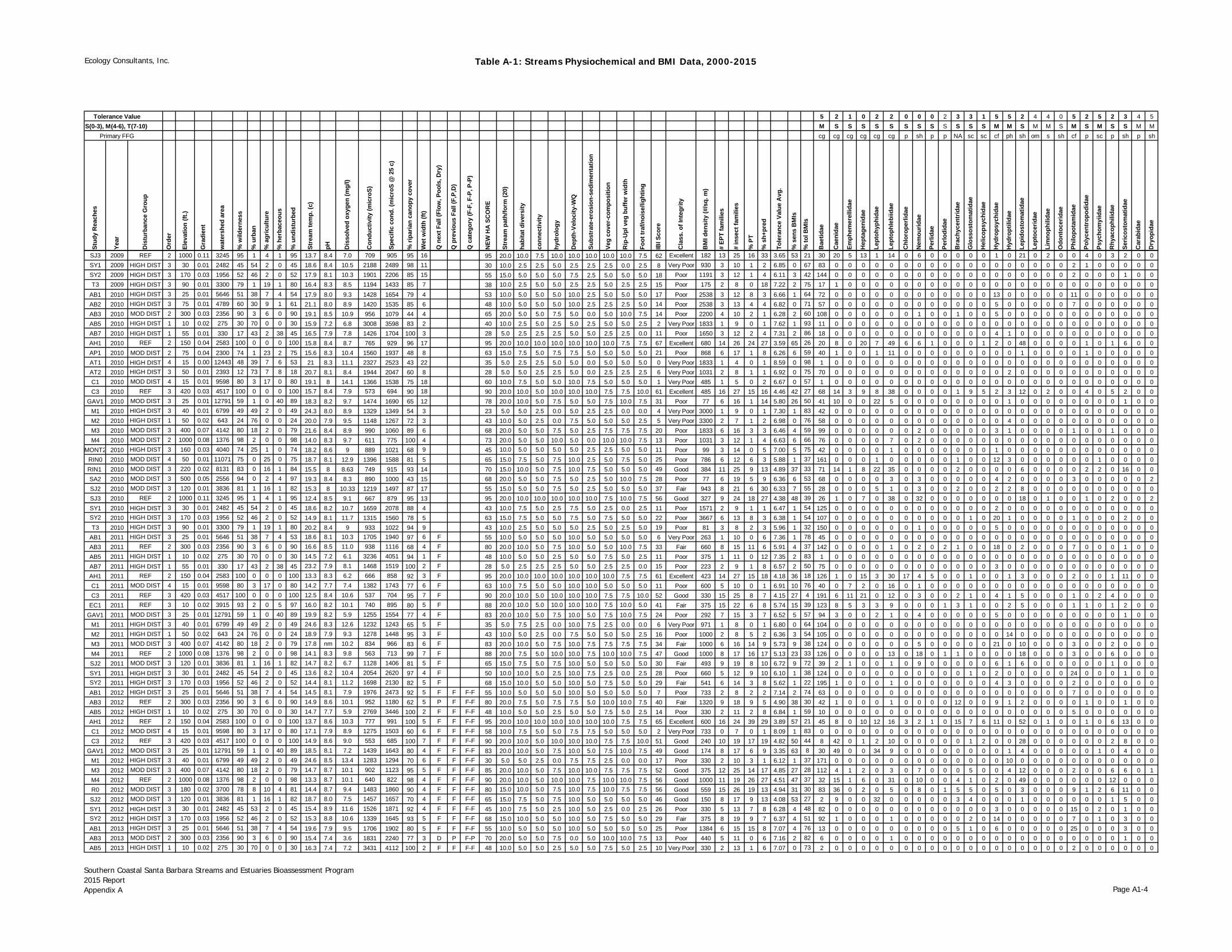
Ecology Consultants, Inc. Table A-1: Streams Physiochemical and BMI Data, 2000-2015
Southern Coastal Santa Barbara Streams and Estuaries Bioassessment Program2015 ReportAppendix A Page A1-4
Tolerance Value 5 2 1 0 2 2 0 0 0 2 3 3 1 5 5 2 4 4 0 5 2 5 2 3 4 5S(0-3), M(4-6), T(7-10) M S S S S S S S S S S S S M M S M M S M S M S S M M
Primary FFG cg cg cg cg cg cg p sh p p NA sc sc cf ph sh om s sh cf p sc p sh p sh
Stud
y R
each
es
Year
Dis
turb
ance
Gro
up
Ord
er
Elev
atio
n (ft
.)
Gra
dien
t
wat
ersh
ed a
rea
% w
ilder
ness
% u
rban
% a
gric
ultu
re
% h
erba
ceou
s
% u
ndis
turb
ed
Stre
am te
mp.
(c)
pH Dis
solv
ed o
xyge
n (m
g/l)
Con
duct
ivity
(mic
roS)
Spec
ific
cond
. (m
icro
S @
25
c)
% ri
paria
n ca
nopy
cov
er
Wet
wid
th (f
t)
Q n
ext F
all (
Flow
, Poo
ls, D
ry)
Q p
revi
ous
Fall
(F,P
,D)
Q c
ateg
ory
(F-F
, F-P
, P-P
)
NEW
HA
SC
OR
E
Stre
am p
ath/
form
(20)
habi
tat d
iver
sity
conn
ectiv
ity
hydr
olog
y
Dep
th-V
eloc
ity-W
Q
Subs
trat
e-er
osio
n-se
dim
enta
tion
Veg
cove
r-co
mpo
sitio
n
Rip
-Upl
veg
buf
fer w
idth
Foot
traf
/noi
se/li
ghtin
g
IBI S
core
Cla
ss. o
f Int
egrit
y
BM
I den
sity
(#/s
q. m
)
# EP
T fa
mili
es
# in
sect
fam
ilies
% P
T
% s
h+pr
ed
Tole
ranc
e Va
lue
Avg
.
% s
ens
BM
Is
% to
l BM
Is
Bae
tidae
Cae
nida
e
Emph
emer
ellid
ae
Hep
tage
nida
e
Lept
ohyp
hida
e
Lept
ophl
ebiid
ae
Chl
orop
erlid
ae
Nem
ourid
ae
Perli
dae
Perlo
dida
e
Bra
chyc
entr
idae
Glo
ssos
tom
atid
ae
Hel
icop
sych
idae
Hyd
rops
ychi
dae
Hyd
ropt
ilida
e
Lepi
dost
omat
idae
Lept
ocer
idae
Lim
noph
ilida
e
Odo
ntoc
erid
ae
Philo
pota
mid
ae
Poly
cent
ropo
dida
e
Psyc
hom
yiid
ae
Rhy
acop
hilid
ae
Seric
osto
mat
idae
Car
abid
ae
Dry
opid
ae
SJ3 2009 REF 2 1000 0.11 3245 95 1 4 1 95 13.7 8.4 7.0 709 905 95 16 95 20.0 10.0 7.5 10.0 10.0 10.0 10.0 10.0 7.5 62 Excellent 182 13 25 16 33 3.65 53 21 30 20 5 13 1 14 0 6 0 0 0 0 0 1 0 21 0 2 0 0 4 0 3 2 0 0SY1 2009 HIGH DIST 3 30 0.01 2482 45 54 2 0 45 18.6 8.4 10.5 2188 2489 98 11 30 10.0 2.5 2.5 5.0 2.5 2.5 2.5 0.0 2.5 8 Very Poor 930 3 10 1 2 6.85 0 67 83 0 0 0 0 0 0 0 0 0 0 0 0 0 0 0 0 0 0 2 1 0 0 0 0 0SY2 2009 HIGH DIST 3 170 0.03 1956 52 46 2 0 52 17.9 8.1 10.3 1901 2206 85 15 55 15.0 5.0 5.0 5.0 7.5 2.5 5.0 5.0 5.0 18 Poor 1191 3 12 1 4 6.11 3 42 144 0 0 0 0 0 0 0 0 0 0 0 0 0 0 0 0 0 0 2 0 0 0 1 0 0T3 2009 HIGH DIST 3 90 0.01 3300 79 1 19 1 80 16.4 8.3 8.5 1194 1433 85 7 38 10.0 2.5 5.0 5.0 2.5 2.5 5.0 2.5 2.5 15 Poor 175 2 8 0 18 7.22 2 75 17 1 0 0 0 0 0 0 0 0 0 0 0 0 0 0 0 0 0 0 0 0 0 0 0 0
AB1 2010 HIGH DIST 3 25 0.01 5646 51 38 7 4 54 17.9 8.0 9.3 1428 1654 79 4 53 10.0 5.0 5.0 5.0 10.0 2.5 5.0 5.0 5.0 17 Poor 2538 3 12 8 3 6.66 1 64 72 0 0 0 0 0 0 0 0 0 0 0 0 13 0 0 0 0 0 11 0 0 0 0 0 0AB2 2010 HIGH DIST 3 75 0.01 4789 60 30 9 1 61 21.1 8.0 8.9 1420 1535 85 6 48 10.0 5.0 5.0 5.0 10.0 2.5 2.5 2.5 5.0 14 Poor 2538 3 13 4 4 6.82 0 71 57 0 0 0 0 0 0 0 0 0 0 0 0 5 0 0 0 0 0 7 0 0 0 0 0 0AB3 2010 MOD DIST 2 300 0.03 2356 90 3 6 0 90 19.1 8.5 10.9 956 1079 44 4 65 20.0 5.0 5.0 7.5 5.0 0.0 5.0 10.0 7.5 14 Poor 2200 4 10 2 1 6.28 2 60 108 0 0 0 0 0 0 1 0 0 1 0 0 5 0 0 0 0 0 0 0 0 0 0 0 0AB5 2010 HIGH DIST 1 10 0.02 275 30 70 0 0 30 15.9 7.2 6.8 3008 3598 83 2 40 10.0 2.5 5.0 2.5 5.0 2.5 5.0 5.0 2.5 2 Very Poor 1833 1 9 0 1 7.62 1 93 11 0 0 0 0 0 0 0 0 0 0 0 0 0 0 0 0 0 0 0 0 0 0 0 0 0AB7 2010 HIGH DIST 1 55 0.01 330 17 43 2 38 45 16.5 7.9 7.8 1426 1704 100 3 28 5.0 2.5 2.5 2.5 5.0 5.0 2.5 2.5 0.0 11 Poor 1650 3 12 2 4 7.31 2 86 18 0 0 0 0 0 0 0 0 0 0 0 0 4 1 0 0 0 0 0 0 0 0 0 0 0AH1 2010 REF 2 150 0.04 2583 100 0 0 0 100 15.8 8.4 8.7 765 929 96 17 95 20.0 10.0 10.0 10.0 10.0 10.0 10.0 7.5 7.5 67 Excellent 680 14 26 24 27 3.59 65 26 20 8 0 20 7 49 6 6 1 0 0 0 1 2 0 48 0 0 0 0 1 0 1 6 0 0AP1 2010 MOD DIST 2 75 0.04 2300 74 1 23 2 75 15.6 8.3 10.4 1560 1937 48 8 63 15.0 7.5 5.0 7.5 7.5 5.0 5.0 5.0 5.0 21 Poor 868 6 17 1 8 6.26 6 59 40 1 0 0 1 11 0 0 0 0 0 0 0 0 0 1 0 0 0 0 1 0 0 0 0 0AT1 2010 HIGH DIST 4 15 0.00 12443 48 39 7 6 53 21 8.3 11.1 2327 2523 43 22 35 5.0 2.5 2.5 5.0 5.0 0.0 5.0 5.0 5.0 0 Very Poor 1833 1 4 0 1 8.59 0 98 1 0 0 0 0 0 0 0 0 0 0 0 0 0 0 0 0 0 0 0 0 0 0 0 0 0AT2 2010 HIGH DIST 3 50 0.01 2393 12 73 7 8 18 20.7 8.1 8.4 1944 2047 60 8 28 5.0 5.0 2.5 2.5 5.0 0.0 2.5 2.5 2.5 6 Very Poor 1031 2 8 1 1 6.92 0 75 70 0 0 0 0 0 0 0 0 0 0 0 0 0 2 0 0 0 0 0 0 0 0 0 0 0C1 2010 MOD DIST 4 15 0.01 9598 80 3 17 0 80 19.1 8 14.1 1366 1538 75 18 60 10.0 7.5 5.0 5.0 10.0 7.5 5.0 5.0 5.0 1 Very Poor 485 1 5 0 2 6.67 0 57 1 0 0 0 0 0 0 0 0 0 0 0 0 0 0 0 0 0 0 0 0 0 0 0 0 0C3 2010 REF 3 420 0.03 4517 100 0 0 0 100 15.7 8.4 7.9 573 694 90 18 90 20.0 10.0 5.0 10.0 10.0 10.0 7.5 7.5 10.0 61 Excellent 485 16 27 15 16 4.46 42 27 68 14 3 9 8 38 0 0 0 0 1 9 5 2 3 12 0 2 0 0 4 0 5 2 0 0
GAV1 2010 MOD DIST 3 25 0.01 12791 59 1 0 40 89 18.3 8.2 9.7 1474 1690 65 12 78 20.0 10.0 5.0 7.5 5.0 5.0 7.5 10.0 7.5 31 Poor 77 6 16 1 14 5.80 26 50 41 10 0 0 22 5 0 0 0 0 0 0 0 0 1 0 0 0 0 0 0 0 0 1 0 0M1 2010 HIGH DIST 3 40 0.01 6799 49 49 2 0 49 24.3 8.0 8.9 1329 1349 54 3 23 5.0 5.0 2.5 0.0 5.0 2.5 2.5 0.0 0.0 4 Very Poor 3000 1 9 0 1 7.30 1 83 42 0 0 0 0 0 0 0 0 0 0 0 0 0 0 0 0 0 0 0 0 0 0 0 0 0M2 2010 HIGH DIST 1 50 0.02 643 24 76 0 0 24 20.0 7.9 9.5 1148 1267 72 3 43 10.0 5.0 2.5 0.0 7.5 5.0 5.0 5.0 2.5 5 Very Poor 3300 2 7 1 2 6.98 0 76 58 0 0 0 0 0 0 0 0 0 0 0 0 0 4 0 0 0 0 0 0 0 0 0 0 0M3 2010 MOD DIST 3 400 0.07 4142 80 18 2 0 79 21.6 8.4 8.9 990 1060 89 6 68 20.0 5.0 5.0 7.5 5.0 2.5 7.5 7.5 7.5 20 Poor 1833 6 16 3 3 6.46 4 59 99 0 0 0 0 0 0 2 0 0 0 0 0 3 1 0 0 0 0 1 0 0 1 0 0 0M4 2010 MOD DIST 2 1000 0.08 1376 98 2 0 0 98 14.0 8.3 9.7 611 775 100 4 73 20.0 5.0 5.0 10.0 5.0 0.0 10.0 10.0 7.5 13 Poor 1031 3 12 1 4 6.63 6 66 76 0 0 0 0 7 0 2 0 0 0 0 0 0 0 0 0 0 0 0 0 0 0 0 0 0
MONT2 2010 HIGH DIST 3 160 0.03 4040 74 25 1 0 74 18.2 8.6 9 889 1021 68 9 45 10.0 5.0 5.0 5.0 5.0 2.5 2.5 5.0 5.0 11 Poor 99 3 14 0 5 7.00 5 75 42 0 0 0 0 1 0 0 0 0 0 0 0 1 0 0 0 0 0 0 0 0 0 0 0 0RIN0 2010 MOD DIST 4 50 0.01 11071 75 0 25 0 75 18.7 8.1 12.9 1396 1588 81 5 65 15.0 7.5 5.0 7.5 10.0 2.5 5.0 7.5 5.0 25 Poor 786 6 12 6 3 5.88 1 37 161 0 0 0 1 0 0 0 0 0 1 0 0 12 3 0 0 0 0 0 0 1 0 0 0 0RIN1 2010 MOD DIST 3 220 0.02 8131 83 0 16 1 84 15.5 8 8.63 749 915 93 14 70 15.0 10.0 5.0 7.5 10.0 7.5 5.0 5.0 5.0 49 Good 384 11 25 9 13 4.89 37 33 71 14 1 8 22 35 0 0 0 0 2 0 0 0 0 6 0 0 0 0 2 2 0 16 0 0SA2 2010 MOD DIST 3 500 0.05 2556 94 0 2 4 97 19.3 8.4 8.3 890 1000 43 15 68 20.0 5.0 5.0 7.5 5.0 2.5 5.0 10.0 7.5 28 Poor 77 6 19 5 9 6.36 6 53 68 0 0 0 0 3 0 3 0 0 0 0 0 4 2 0 0 0 0 3 0 0 0 0 0 2SJ2 2010 MOD DIST 3 120 0.01 3836 81 1 16 1 82 15.3 8 10.33 1219 1497 87 17 55 15.0 5.0 5.0 7.5 5.0 2.5 5.0 5.0 5.0 37 Fair 943 8 21 6 30 6.33 7 55 28 0 0 0 5 1 0 3 0 0 2 0 0 2 2 8 0 0 0 0 0 0 0 0 0 0SJ3 2010 REF 2 1000 0.11 3245 95 1 4 1 95 12.4 8.5 9.1 667 879 95 13 95 20.0 10.0 10.0 10.0 10.0 10.0 7.5 10.0 7.5 56 Good 327 9 24 18 27 4.38 48 39 26 1 0 7 0 38 0 32 0 0 0 0 0 0 0 18 0 1 0 0 1 0 2 0 0 2SY1 2010 HIGH DIST 3 30 0.01 2482 45 54 2 0 45 18.6 8.2 10.7 1659 2078 88 4 43 10.0 7.5 5.0 2.5 7.5 5.0 2.5 0.0 2.5 11 Poor 1571 2 9 1 1 6.47 1 54 125 0 0 0 0 0 0 0 0 0 0 0 0 2 0 0 0 0 0 0 0 0 0 0 0 0SY2 2010 HIGH DIST 3 170 0.03 1956 52 46 2 0 52 14.9 8.1 11.7 1315 1560 78 5 63 15.0 7.5 5.0 5.0 7.5 5.0 7.5 5.0 5.0 22 Poor 3667 6 13 8 3 6.38 1 54 107 0 0 0 0 0 0 0 0 0 0 1 0 20 1 0 0 0 0 1 0 0 0 2 0 0T3 2010 HIGH DIST 3 90 0.01 3300 79 1 19 1 80 20.2 8.4 9 933 1022 94 9 43 10.0 2.5 5.0 5.0 5.0 2.5 5.0 2.5 5.0 19 Poor 81 3 8 2 3 5.96 1 32 150 0 0 0 0 0 0 1 0 0 0 0 0 5 0 0 0 0 0 0 0 0 0 0 0 0
AB1 2011 HIGH DIST 3 25 0.01 5646 51 38 7 4 53 18.6 8.1 10.3 1705 1940 97 6 F 55 10.0 5.0 5.0 5.0 10.0 5.0 5.0 5.0 5.0 6 Very Poor 263 1 10 0 6 7.36 1 78 45 0 0 0 0 0 0 0 0 0 0 0 0 0 0 0 0 0 0 0 0 0 0 0 0 0AB3 2011 REF 2 300 0.03 2356 90 3 6 0 90 16.6 8.5 11.0 938 1116 68 4 F 80 20.0 10.0 5.0 7.5 10.0 5.0 5.0 10.0 7.5 33 Fair 660 8 15 11 6 5.91 4 37 142 0 0 0 0 1 0 2 0 2 1 0 0 18 0 2 0 0 0 7 0 0 0 1 0 0AB5 2011 HIGH DIST 1 10 0.02 275 30 70 0 0 30 14.5 7.2 6.1 3236 4051 94 1 F 48 10.0 5.0 5.0 2.5 5.0 5.0 7.5 5.0 2.5 11 Poor 375 1 11 0 12 7.35 2 83 1 0 0 0 0 0 0 0 0 0 0 0 0 0 0 0 0 0 0 0 0 0 0 0 0 0AB7 2011 HIGH DIST 1 55 0.01 330 17 43 2 38 45 23.2 7.9 8.1 1468 1519 100 2 F 28 5.0 2.5 2.5 2.5 5.0 5.0 2.5 2.5 0.0 15 Poor 223 2 9 1 8 6.57 2 50 75 0 0 0 0 0 0 0 0 0 0 0 0 3 0 0 0 0 0 0 0 0 0 0 0 0AH1 2011 REF 2 150 0.04 2583 100 0 0 0 100 13.3 8.3 6.2 666 858 92 3 F 95 20.0 10.0 10.0 10.0 10.0 10.0 10.0 7.5 7.5 61 Excellent 423 14 27 15 18 4.18 36 18 126 1 0 15 3 30 17 4 5 0 0 1 0 0 1 3 0 0 0 2 0 0 1 11 0 0C1 2011 MOD DIST 4 15 0.01 9598 80 3 17 0 80 14.2 7.7 7.4 1382 1743 77 6 F 63 10.0 7.5 5.0 5.0 10.0 10.0 5.0 5.0 5.0 11 Poor 600 5 10 0 1 6.91 10 76 40 0 7 2 0 16 0 1 0 0 0 0 0 0 0 0 0 0 0 0 0 0 0 0 0 0C3 2011 REF 3 420 0.03 4517 100 0 0 0 100 12.5 8.4 10.6 537 704 95 7 F 90 20.0 10.0 5.0 10.0 10.0 10.0 7.5 7.5 10.0 52 Good 330 15 25 8 7 4.15 27 4 191 6 11 21 0 12 0 3 0 0 2 1 0 4 1 5 0 0 0 1 0 2 4 0 0 0
EC1 2011 REF 3 10 0.02 3915 93 2 0 5 97 16.0 8.2 10.1 740 895 80 5 F 88 20.0 10.0 5.0 10.0 10.0 10.0 7.5 10.0 5.0 41 Fair 375 15 22 6 8 5.74 15 39 123 8 5 3 3 9 0 0 0 1 3 1 0 0 2 5 0 0 0 1 1 0 1 2 0 0GAV1 2011 MOD DIST 3 25 0.01 12791 59 1 0 40 89 19.9 8.2 5.9 1255 1554 77 4 F 83 20.0 10.0 5.0 7.5 10.0 5.0 7.5 10.0 7.5 24 Poor 292 7 15 3 7 6.52 5 57 94 3 0 0 2 1 0 4 0 0 0 0 0 5 0 0 0 0 0 0 0 0 0 1 0 0
M1 2011 HIGH DIST 3 40 0.01 6799 49 49 2 0 49 24.6 8.3 12.6 1232 1243 65 5 F 35 5.0 7.5 2.5 0.0 10.0 7.5 2.5 0.0 0.0 6 Very Poor 971 1 8 0 1 6.80 0 64 104 0 0 0 0 0 0 0 0 0 0 0 0 0 0 0 0 0 0 0 0 0 0 0 0 0M2 2011 HIGH DIST 1 50 0.02 643 24 76 0 0 24 18.9 7.9 9.3 1278 1448 95 3 F 43 10.0 5.0 2.5 0.0 7.5 5.0 5.0 5.0 2.5 16 Poor 1000 2 8 5 2 6.36 3 54 105 0 0 0 0 0 0 0 0 0 0 0 0 0 14 0 0 0 0 0 0 0 0 0 0 0M3 2011 MOD DIST 3 400 0.07 4142 80 18 2 0 79 17.8 nm 10.2 834 966 83 6 F 83 20.0 10.0 5.0 7.5 10.0 7.5 7.5 7.5 7.5 34 Fair 1000 6 16 14 9 5.73 9 38 124 0 0 0 0 0 0 5 0 0 0 0 0 21 0 10 0 0 0 3 0 0 2 0 0 0M4 2011 REF 2 1000 0.08 1376 98 2 0 0 98 14.1 8.3 9.8 563 713 99 7 F 88 20.0 7.5 5.0 10.0 10.0 7.5 10.0 10.0 7.5 47 Good 1000 8 17 16 17 5.13 23 33 126 0 0 0 0 13 0 18 0 1 1 0 0 0 0 18 0 0 0 3 0 0 6 0 0 0SJ2 2011 MOD DIST 3 120 0.01 3836 81 1 16 1 82 14.7 8.2 6.7 1128 1406 81 5 F 65 15.0 7.5 5.0 7.5 10.0 5.0 5.0 5.0 5.0 30 Fair 493 9 19 8 10 6.72 9 72 39 2 1 0 0 1 0 9 0 0 0 0 0 6 1 6 0 0 0 0 0 0 1 0 0 0SY1 2011 HIGH DIST 3 30 0.01 2482 45 54 2 0 45 13.6 8.2 10.4 2054 2620 97 4 F 50 10.0 10.0 5.0 2.5 10.0 7.5 2.5 0.0 2.5 28 Poor 660 5 12 9 10 6.10 1 38 124 0 0 0 0 0 0 0 0 0 0 1 0 2 0 0 0 0 0 24 0 0 0 1 0 0SY2 2011 HIGH DIST 3 170 0.03 1956 52 46 2 0 52 14.4 8.1 11.2 1698 2130 82 5 F 68 15.0 10.0 5.0 5.0 10.0 5.0 7.5 5.0 5.0 29 Fair 541 6 14 3 8 5.62 1 22 195 1 0 0 0 1 0 0 0 0 0 0 0 4 3 0 0 0 0 2 0 0 0 0 0 0AB1 2012 HIGH DIST 3 25 0.01 5646 51 38 7 4 54 14.5 8.1 7.9 1976 2473 92 5 F F F-F 55 10.0 5.0 5.0 5.0 10.0 5.0 5.0 5.0 5.0 7 Poor 733 2 8 2 2 7.14 2 74 63 0 0 0 0 0 0 0 0 0 0 0 0 0 0 0 0 0 0 7 0 0 0 0 0 0AB3 2012 REF 2 300 0.03 2356 90 3 6 0 90 14.9 8.6 10.1 952 1180 62 5 P F F-F 80 20.0 7.5 5.0 7.5 7.5 5.0 10.0 10.0 7.5 40 Fair 1320 9 18 9 5 4.90 38 30 42 1 0 0 0 1 0 0 0 0 12 0 0 9 1 2 0 0 0 0 1 0 0 1 0 0AB5 2012 HIGH DIST 1 10 0.02 275 30 70 0 0 30 14.7 7.7 5.9 2769 3446 100 2 F F F-F 48 10.0 5.0 5.0 2.5 5.0 5.0 7.5 5.0 2.5 14 Poor 330 2 11 2 8 6.84 1 59 10 0 0 0 0 0 0 0 0 0 0 0 0 0 0 0 0 0 0 5 0 0 0 0 0 0AH1 2012 REF 2 150 0.04 2583 100 0 0 0 100 13.7 8.6 10.3 777 991 100 5 F F F-F 95 20.0 10.0 10.0 10.0 10.0 10.0 10.0 7.5 7.5 65 Excellent 600 16 24 39 29 3.89 57 21 45 8 0 10 12 16 3 2 1 0 15 7 6 11 0 52 0 1 0 0 1 0 6 13 0 0C1 2012 MOD DIST 4 15 0.01 9598 80 3 17 0 80 17.1 7.9 8.9 1275 1503 60 6 F F F-F 58 10.0 7.5 5.0 5.0 7.5 7.5 5.0 5.0 5.0 2 Very Poor 733 0 7 0 1 8.09 1 83 0 0 0 0 0 0 0 0 0 0 0 0 0 0 0 0 0 0 0 0 0 0 0 0 0 0C3 2012 REF 3 420 0.03 4517 100 0 0 0 100 14.9 8.6 9.0 553 685 100 7 F F F-F 90 20.0 10.0 5.0 10.0 10.0 10.0 7.5 7.5 10.0 51 Good 240 10 19 17 19 4.82 50 44 8 42 0 1 2 10 0 0 0 0 0 1 2 0 0 28 0 0 0 0 0 0 2 8 0 0
GAV1 2012 MOD DIST 3 25 0.01 12791 59 1 0 40 89 18.5 8.1 7.2 1439 1643 80 4 F F F-F 83 20.0 10.0 5.0 7.5 10.0 5.0 7.5 10.0 7.5 49 Good 174 8 17 6 9 3.35 63 8 30 49 0 0 34 9 0 0 0 0 0 0 0 0 1 4 0 0 0 0 0 1 0 4 0 0M1 2012 HIGH DIST 3 40 0.01 6799 49 49 2 0 49 24.6 8.5 13.4 1283 1294 70 6 F F F-F 30 5.0 5.0 2.5 0.0 7.5 7.5 2.5 0.0 0.0 17 Poor 330 2 10 3 1 6.12 1 37 171 0 0 0 0 0 0 0 0 0 0 0 0 0 10 0 0 0 0 0 0 0 0 0 0 0M3 2012 MOD DIST 3 400 0.07 4142 80 18 2 0 79 14.7 8.7 10.1 902 1123 95 5 F F F-F 85 20.0 10.0 5.0 7.5 10.0 10.0 7.5 7.5 7.5 52 Good 375 12 25 14 17 4.85 27 28 112 4 1 2 0 3 0 7 0 0 0 5 0 0 4 12 0 0 0 2 0 0 6 6 0 1M4 2012 REF 2 1000 0.08 1376 98 2 0 0 98 13.3 8.7 10.1 640 822 98 4 F F F-F 90 20.0 10.0 5.0 10.0 10.0 7.5 10.0 10.0 7.5 56 Good 1000 11 19 26 27 4.51 47 37 32 15 1 6 0 31 0 10 0 0 4 1 0 2 0 49 0 0 0 0 0 0 12 0 0 0R0 2012 MOD DIST 3 180 0.02 3700 78 8 10 4 81 14.4 8.7 9.4 1483 1860 90 4 F F F-F 80 15.0 10.0 5.0 7.5 10.0 7.5 10.0 7.5 7.5 56 Good 559 15 26 19 13 4.94 31 30 83 36 0 2 0 5 0 8 0 1 5 5 0 5 0 3 0 0 0 9 1 2 6 11 0 0SJ2 2012 MOD DIST 3 120 0.01 3836 81 1 16 1 82 18.7 8.0 7.5 1457 1657 70 4 F F F-F 65 15.0 7.5 5.0 7.5 10.0 5.0 5.0 5.0 5.0 46 Good 150 8 17 9 13 4.08 53 27 2 9 0 0 32 0 0 0 0 0 3 4 0 0 0 1 0 0 0 0 0 0 1 5 0 0SY1 2012 HIGH DIST 3 30 0.01 2482 45 53 2 0 45 15.4 8.9 11.6 1526 1871 92 4 F F F-F 45 10.0 7.5 5.0 2.5 10.0 5.0 2.5 0.0 2.5 26 Poor 330 5 13 7 8 6.28 4 48 82 0 0 0 0 0 0 0 0 0 0 0 0 3 0 0 0 0 0 15 0 2 0 1 0 0SY2 2012 HIGH DIST 3 170 0.03 1956 52 46 2 0 52 15.3 8.8 10.6 1339 1645 93 5 F F F-F 68 15.0 10.0 5.0 5.0 10.0 5.0 7.5 5.0 5.0 29 Fair 375 8 19 9 7 6.37 4 51 92 1 0 0 0 1 0 0 0 0 0 2 0 14 0 0 0 0 0 7 0 1 0 3 0 0AB1 2013 HIGH DIST 3 25 0.01 5646 51 38 7 4 54 19.6 7.9 9.5 1706 1902 80 5 F F F-F 55 10.0 5.0 5.0 5.0 10.0 5.0 5.0 5.0 5.0 25 Poor 1384 6 15 15 8 7.07 4 76 13 0 0 0 0 0 0 0 0 0 5 1 0 6 0 0 0 0 0 25 0 0 0 3 0 0AB3 2013 MOD DIST 2 300 0.03 2356 90 3 6 0 90 15.4 7.4 3.6 1831 2240 77 3 D P F-P 70 20.0 5.0 5.0 7.5 0.0 5.0 10.0 10.0 7.5 13 Poor 440 5 11 0 6 7.16 2 82 6 0 0 0 0 1 0 0 0 0 0 0 0 0 0 0 0 0 0 0 0 0 0 1 0 0AB5 2013 HIGH DIST 1 10 0.02 275 30 70 0 0 30 16.3 7.4 7.2 3431 4112 100 2 F F F-F 48 10.0 5.0 5.0 2.5 5.0 5.0 7.5 5.0 2.5 10 Very Poor 330 2 13 1 6 7.07 0 73 2 0 0 0 0 0 0 0 0 0 0 0 0 0 0 0 0 0 0 2 0 0 0 0 0 0

Ecology Consultants, Inc. Table A-1: Streams Physiochemical and BMI Data, 2000-2015
Southern Coastal Santa Barbara Streams and Estuaries Bioassessment Program2015 ReportAppendix A Page A1-5
Tolerance Value 5 2 1 0 2 2 0 0 0 2 3 3 1 5 5 2 4 4 0 5 2 5 2 3 4 5S(0-3), M(4-6), T(7-10) M S S S S S S S S S S S S M M S M M S M S M S S M M
Primary FFG cg cg cg cg cg cg p sh p p NA sc sc cf ph sh om s sh cf p sc p sh p sh
Stud
y R
each
es
Year
Dis
turb
ance
Gro
up
Ord
er
Elev
atio
n (ft
.)
Gra
dien
t
wat
ersh
ed a
rea
% w
ilder
ness
% u
rban
% a
gric
ultu
re
% h
erba
ceou
s
% u
ndis
turb
ed
Stre
am te
mp.
(c)
pH Dis
solv
ed o
xyge
n (m
g/l)
Con
duct
ivity
(mic
roS)
Spec
ific
cond
. (m
icro
S @
25
c)
% ri
paria
n ca
nopy
cov
er
Wet
wid
th (f
t)
Q n
ext F
all (
Flow
, Poo
ls, D
ry)
Q p
revi
ous
Fall
(F,P
,D)
Q c
ateg
ory
(F-F
, F-P
, P-P
)
NEW
HA
SC
OR
E
Stre
am p
ath/
form
(20)
habi
tat d
iver
sity
conn
ectiv
ity
hydr
olog
y
Dep
th-V
eloc
ity-W
Q
Subs
trat
e-er
osio
n-se
dim
enta
tion
Veg
cove
r-co
mpo
sitio
n
Rip
-Upl
veg
buf
fer w
idth
Foot
traf
/noi
se/li
ghtin
g
IBI S
core
Cla
ss. o
f Int
egrit
y
BM
I den
sity
(#/s
q. m
)
# EP
T fa
mili
es
# in
sect
fam
ilies
% P
T
% s
h+pr
ed
Tole
ranc
e Va
lue
Avg
.
% s
ens
BM
Is
% to
l BM
Is
Bae
tidae
Cae
nida
e
Emph
emer
ellid
ae
Hep
tage
nida
e
Lept
ohyp
hida
e
Lept
ophl
ebiid
ae
Chl
orop
erlid
ae
Nem
ourid
ae
Perli
dae
Perlo
dida
e
Bra
chyc
entr
idae
Glo
ssos
tom
atid
ae
Hel
icop
sych
idae
Hyd
rops
ychi
dae
Hyd
ropt
ilida
e
Lepi
dost
omat
idae
Lept
ocer
idae
Lim
noph
ilida
e
Odo
ntoc
erid
ae
Philo
pota
mid
ae
Poly
cent
ropo
dida
e
Psyc
hom
yiid
ae
Rhy
acop
hilid
ae
Seric
osto
mat
idae
Car
abid
ae
Dry
opid
ae
AH1 2013 REF 2 150 0.04 2583 100 0 0 0 100 14.7 7.6 8.4 1099 100 3 F F F-F 95 20.0 10.0 10.0 10.0 10.0 10.0 10.0 7.5 7.5 65 Excellent 600 16 32 21 18 4.13 55 29 11 30 0 4 26 8 1 8 1 0 0 2 2 11 1 17 0 0 0 5 7 0 7 0 0 0C1 2013 MOD DIST 4 15 0.01 9598 80 3 17 0 80 15.8 7.6 6.2 1568 75 5 P F F-F 58 10.0 7.5 5.0 5.0 7.5 7.5 5.0 5.0 5.0 2 Very Poor 173 1 3 0 1 7.88 2 81 1 0 0 0 0 0 0 0 0 0 0 0 0 0 0 0 0 0 0 0 0 0 0 0 0 0C3 2013 REF 3 420 0.03 4517 100 0 0 0 100 13.0 7.9 9.0 795 89 5 P F F-F 90 20.0 10.0 5.0 10.0 10.0 10.0 7.5 7.5 10.0 46 Good 398 9 22 13 17 5.40 36 53 15 48 5 0 7 0 0 0 0 0 0 0 1 1 0 33 0 0 0 0 0 0 3 1 0 0
GAV1 2013 MOD DIST 3 25 0.01 12791 59 1 0 40 89 14.6 7.5 8.1 2029 58 3 P F F-F 85 20.0 10.0 5.0 7.5 10.0 5.0 10.0 10.0 7.5 54 Good 1065 9 16 17 27 4.17 55 35 4 53 0 0 45 3 0 28 0 0 3 0 0 0 0 14 0 0 0 0 2 0 0 3 0 0M1 2013 HIGH DIST 3 40 0.01 6799 49 49 2 0 49 23.3 7.7 9.0 1423 1471 67 5 F F F-F 30 5.0 5.0 2.5 0.0 7.5 7.5 2.5 0.0 0.0 3 Very Poor 750 2 5 0 4 7.76 0 93 8 0 0 0 0 0 0 0 0 0 1 0 0 0 0 0 0 0 0 0 0 0 0 0 0 0M2 2013 HIGH DIST 1 50 0.02 643 24 76 0 0 24 18.5 8.0 9.5 1274 1454 95 3 F F F-F 40 10.0 5.0 2.5 0.0 5.0 5.0 5.0 5.0 2.5 9 Very Poor 1065 1 5 2 7 6.05 4 40 0 0 0 0 0 0 0 0 0 0 0 0 0 0 6 0 0 0 0 0 0 0 0 0 0 0M3 2013 MOD DIST 3 400 0.07 4142 80 18 2 0 79 15.6 7.6 6.3 991 1209 95 4 P F F-F 83 20.0 10.0 5.0 7.5 7.5 10.0 7.5 7.5 7.5 32 Fair 440 9 17 5 11 6.07 18 69 1 6 0 2 0 13 0 2 0 0 1 2 0 2 0 0 0 0 0 0 0 0 7 0 0 0M4 2013 REF 2 1000 0.08 1376 98 2 0 0 98 15.4 7.9 9.1 797 976 93 4 P F F-F 90 20.0 10.0 5.0 10.0 7.5 10.0 10.0 10.0 7.5 43 Fair 750 12 26 9 12 5.61 33 58 1 27 4 2 0 25 0 4 0 0 0 6 0 2 0 7 0 0 0 0 5 1 1 0 0 0SA2 2013 REF 3 500 0.05 2556 94 0 2 4 97 19.2 7.5 7.0 1623 93 3 P F F-F 80 20.0 10.0 5.0 7.5 7.5 5.0 7.5 10.0 7.5 32 Fair 213 6 16 1 12 5.17 31 38 7 2 0 1 0 50 0 0 0 0 1 0 0 0 0 0 0 0 0 0 0 0 0 2 0 0SJ2 2013 MOD DIST 3 120 0.01 3836 81 1 16 1 82 17.6 7.5 9.0 2360 77 2 F F F-F 65 15.0 7.5 5.0 7.5 10.0 5.0 5.0 5.0 5.0 45 Fair 166 8 16 23 25 5.57 37 56 1 4 0 0 10 0 0 1 0 0 0 2 0 1 0 0 0 0 0 0 1 0 0 34 0 0SY1 2013 HIGH DIST 3 30 0.01 2482 45 53 2 0 45 16.1 8.0 7.3 2463 2969 98 2 D F F-F 40 10.0 7.5 5.0 2.5 5.0 5.0 2.5 0.0 2.5 20 Poor 660 5 11 5 9 5.43 4 23 4 0 0 0 0 0 0 0 0 0 1 0 0 11 0 0 0 0 0 0 0 1 0 3 0 0SY2 2013 HIGH DIST 3 170 0.03 1956 52 46 2 0 52 16.2 7.6 8.0 1762 2121 95 4 P F F-F 68 15.0 10.0 5.0 5.0 10.0 5.0 7.5 5.0 5.0 31 Fair 750 5 15 17 15 6.52 11 62 7 0 0 0 0 0 0 0 0 0 6 0 0 30 0 0 0 0 0 0 0 0 1 13 0 0AB1 2014 HIGH DIST 3 25 0.01 5646 51 38 7 4 54 17.9 7.9 10.8 1646 72 5 F F F-F 53 10.0 5.0 5.0 5.0 7.5 5.0 5.0 5.0 5.0 15 Poor 1205 4 11 5 2 6.99 1 69 55 0 0 0 0 0 0 0 0 0 0 1 0 13 0 0 0 0 0 0 0 0 0 0 0 0AB3 2014 MOD DIST 2 300 0.03 2356 90 3 6 0 90 15.3 7.8 8.2 1934 77 5 D D F-P 73 20.0 5.0 5.0 7.5 5.0 2.5 10.0 10.0 7.5 12 Poor 185 2 11 1 8 7.04 3 85 8 0 0 0 0 0 0 0 0 0 0 0 0 0 1 0 0 0 0 0 0 0 0 0 0 0AB5 2014 HIGH DIST 1 10 0.02 275 30 70 0 0 30 15.4 7.2 6.1 3371 100 2 F F F-F 48 10.0 5.0 5.0 2.5 5.0 5.0 7.5 5.0 2.5 4 Very Poor 255 1 5 0 4 6.78 0 71 1 0 0 0 0 0 0 0 0 0 0 0 0 0 0 0 0 0 0 0 0 0 0 0 0 0AH1 2014 REF 2 150 0.04 2583 100 0 0 0 100 12.8 8.1 9.7 1246 94 3 F F F-F 95 20.0 10.0 10.0 10.0 10.0 10.0 10.0 7.5 7.5 47 Good 901 14 23 19 13 5.57 27 52 17 28 0 2 3 13 5 5 2 3 0 0 0 0 3 4 0 0 0 28 0 0 3 3 0 0C1 2014 MOD DIST 4 15 0.01 9598 80 3 17 0 80 15.6 7.5 6.5 1835 85 3 P P F-P 55 10.0 7.5 5.0 5.0 5.0 7.5 5.0 5.0 5.0 7 Very Poor 241 0 6 0 6 6.78 2 74 0 0 0 0 0 0 0 0 0 0 0 0 0 0 0 0 0 0 0 0 0 0 0 0 0 0C3 2014 REF 3 420 0.03 4517 100 0 0 0 100 13.3 7.9 9.1 1000 99 5 P P F-P 88 20.0 10.0 5.0 10.0 7.5 10.0 7.5 7.5 10.0 24 Poor 390 11 18 3 3 6.36 14 75 23 1 1 3 0 28 0 2 0 2 0 0 1 1 1 0 0 0 0 2 0 0 0 0 0 0
GAV1 2014 MOD DIST 3 25 0.01 12791 59 1 0 40 89 14.1 7.5 7.3 2778 62 2 P P F-P 83 20.0 10.0 5.0 7.5 7.5 5.0 10.0 10.0 7.5 14 Poor 206 4 11 1 8 6.98 5 72 9 0 0 0 0 2 0 0 0 1 1 0 0 0 0 0 0 0 0 0 0 0 0 0 0 0M1 2014 HIGH DIST 3 40 0.01 6799 49 49 2 0 49 18.6 7.7 11.2 1433 55 3 F F F-F 28 5.0 5.0 2.5 0.0 5.0 7.5 2.5 0.0 0.0 3 Very Poor 159 0 3 0 6 7.74 0 93 0 0 0 0 0 0 0 0 0 0 0 0 0 0 0 0 0 0 0 0 0 0 0 0 0 0M2 2014 HIGH DIST 1 50 0.02 643 24 76 0 0 24 19.3 8.1 9.3 1465 95 2 F F F-F 40 10.0 5.0 2.5 0.0 5.0 5.0 5.0 5.0 2.5 3 Very Poor 300 0 4 0 7 7.52 0 85 0 0 0 0 0 0 0 0 0 0 0 0 0 0 0 0 0 0 0 0 0 0 0 0 0 0M3 2014 MOD DIST 3 400 0.07 4142 80 18 2 0 79 15.9 7.8 8.5 1280 85 4 P P F-P 83 20.0 10.0 5.0 7.5 7.5 10.0 7.5 7.5 7.5 27 Poor 319 8 20 3 10 6.55 15 75 2 14 0 1 0 11 0 0 0 0 0 0 0 0 0 3 0 0 0 1 0 0 1 4 0 0M4 2014 REF 2 1000 0.08 1376 98 2 0 0 98 16.8 7.7 6.3 953 100 4 P P F-P 88 20.0 10.0 5.0 10.0 5.0 10.0 10.0 10.0 7.5 28 Poor 400 7 22 2 11 6.22 16 72 7 17 1 0 0 15 0 4 0 0 0 0 0 0 0 0 0 0 0 1 0 0 0 1 0 0SJ2 2014 MOD DIST 3 120 0.01 3836 81 1 16 1 82 16.9 7.8 9.4 2228 93 4 F F F-F 63 15.0 7.5 5.0 7.5 7.5 5.0 5.0 5.0 5.0 26 Poor 938 10 22 7 6 6.94 6 75 29 3 0 0 0 1 0 1 0 0 1 4 0 5 0 0 0 0 0 8 0 0 1 2 0 0SY2 2014 HIGH DIST 3 170 0.03 1956 52 46 2 0 52 14.7 7.7 8.2 2618 83 5 P P F-P 65 15.0 10.0 5.0 5.0 7.5 5.0 7.5 5.0 5.0 25 Poor 800 7 15 4 13 6.65 5 67 36 3 0 0 0 2 0 0 0 0 0 0 0 7 0 0 0 0 0 1 0 0 2 2 0 0AB1 2015 HIGH DIST 3 25 0.01 5646 51 38 7 4 54 15.9 7.9 8.9 1559 1886 85 10 F F F-F 55 10.0 7.5 5.0 2.5 7.5 5.0 7.5 5.0 5.0 17 Poor 1200 4 11 4 6 6.77 1 66 33 0 0 0 0 0 0 0 0 0 0 0 0 7 1 0 0 0 0 4 0 0 0 0 0 0AB5 2015 HIGH DIST 1 10 0.02 275 30 70 0 0 30 14.9 7.2 5.5 3295 4089 100 4 F F F-F 45 10.0 5.0 5.0 2.5 2.5 5.0 7.5 5.0 2.5 5 Very Poor 252 0 13 0 3 7.55 1 97 0 0 0 0 0 0 0 0 0 0 0 0 0 0 0 0 0 0 0 0 0 0 0 0 0 0AB7 2015 HIGH DIST 1 55 0.01 330 17 43 2 38 45 15.9 7.9 8.9 1404 1699 93 4 F F F-F 28 5.0 2.5 2.5 2.5 5.0 5.0 2.5 2.5 0.0 23 Poor 625 2 10 2 28 6.47 2 63 7 0 0 0 0 0 0 0 0 0 0 0 0 0 6 0 0 0 0 0 0 0 0 0 0 0AB8 2015 HIGH DIST 1 57 0.01 332 17 43 2 38 45 15.4 7.9 10.5 1880 2305 92 4 P F F-F 28 5.0 2.5 2.5 2.5 5.0 5.0 2.5 2.5 0.0 13 Poor 341 1 8 0 16 7.02 2 82 0 0 0 0 0 0 0 0 0 0 0 0 0 1 0 0 0 0 0 0 0 0 0 0 0 0AH0 2015 MOD DIST 2 40 0.02 2817 100 0 0 0 100 16.6 7.1 2.1 1092 1301 100 6 P P P-P 70 15.0 10.0 5.0 10.0 2.5 7.5 7.5 5.0 7.5 3 Very Poor 536 2 6 0 2 7.67 1 92 14 1 0 0 0 0 0 0 0 0 0 0 0 0 0 0 0 0 0 0 0 0 0 0 0 0AH1 2015 REF 2 150 0.04 2583 100 0 0 0 100 15.0 8.1 10.3 1126 1387 99 10 F F F-F 93 20.0 10.0 10.0 10.0 7.5 10.0 10.0 7.5 7.5 55 Good 682 15 27 16 12 4.84 33 33 66 24 0 5 8 20 0 5 1 1 0 2 0 16 1 10 0 0 0 7 0 0 4 1 0 0C1 2015 MOD DIST 4 15 0.01 9598 80 3 17 0 80 17.0 7.6 6.7 1551 1821 90 6 P P F-P 55 10.0 7.5 5.0 5.0 5.0 7.5 5.0 5.0 5.0 5 Very Poor 115 1 6 0 6 7.74 1 94 1 0 0 0 0 0 0 0 0 0 0 0 0 0 0 0 0 0 0 0 0 0 0 0 0 0C3 2015 REF 3 420 0.03 4517 100 0 0 0 100 13.4 7.9 8.1 871 1120 95 10 D P F-P 85 20.0 10.0 5.0 10.0 5.0 10.0 7.5 7.5 10.0 14 Poor 750 2 11 0 5 6.59 19 76 3 0 0 0 0 55 0 0 0 0 0 0 0 0 0 0 0 0 0 0 0 0 0 0 0 0
GAV1 2015 MOD DIST 3 25 0.01 12791 59 1 0 40 89 15.1 7.7 7.3 2518 3111 94 13 P P F-P 80 20.0 10.0 5.0 7.5 5.0 5.0 10.0 10.0 7.5 11 Poor 271 2 13 0 7 7.35 5 85 11 0 0 0 0 6 0 0 0 0 0 0 0 0 0 0 0 0 0 0 0 0 0 0 0 0LC1 2015 MOD DIST 2 320 0.06 1024 89 0 0 11 97 14.3 8.2 10.4 838 1054 94 11 F F F-F 70 15.0 10.0 5.0 10.0 7.5 5.0 7.5 5.0 5.0 43 Fair 600 10 23 12 16 5.93 21 65 9 3 0 0 0 11 0 3 0 0 0 0 0 9 2 13 0 0 0 0 1 0 1 6 0 0M1 2015 HIGH DIST 3 40 0.01 6799 49 49 2 0 49 16.0 7.4 2.2 987 1193 68 8 P F P-P 23 5.0 5.0 2.5 0.0 0.0 7.5 2.5 0.0 0.0 0 Very Poor 800 0 3 0 1 8.43 0 98 0 0 0 0 0 0 0 0 0 0 0 0 0 0 0 0 0 0 0 0 0 0 0 0 0 0M2 2015 HIGH DIST 1 50 0.02 643 24 76 0 0 24 18.9 8.2 9.8 1267 1436 91 4 F F F-F 40 10.0 5.0 2.5 0.0 5.0 5.0 5.0 5.0 2.5 9 Very Poor 600 2 7 1 3 6.87 2 87 9 0 0 0 0 0 0 0 0 0 0 0 0 0 3 0 0 0 0 0 0 0 0 0 0 0M3 2015 MOD DIST 3 400 0.07 4142 80 18 2 0 79 15.6 7.9 9.2 941 1148 93 7 P P F-P 80 20.0 10.0 5.0 7.5 5.0 10.0 7.5 7.5 7.5 32 Fair 750 5 19 9 12 6.48 12 73 0 0 0 0 0 10 0 4 0 0 0 0 0 17 0 5 0 0 0 0 0 0 1 0 0 0M4 2015 REF 2 1000 0.08 1376 98 2 0 0 98 15.6 7.4 2.5 na na 98 3 D P P-P 85 20.0 10.0 7.5 10.0 0.0 10.0 10.0 10.0 7.5 4 Very Poor 300 2 7 0 1 7.37 1 96 3 0 0 0 0 1 0 0 0 0 0 0 0 0 0 0 0 0 0 0 0 0 0 0 0 0SJ2 2015 MOD DIST 3 120 0.01 3836 81 1 16 1 82 14.5 7.8 8.9 1867 2337 72 10 F F F-F 63 15.0 7.5 5.0 7.5 7.5 5.0 5.0 5.0 5.0 40 Fair 533 8 21 24 19 6.40 6 53 7 1 0 0 0 0 0 0 0 1 2 0 0 58 1 0 0 0 0 8 0 0 0 3 0 0SY2 2015 HIGH DIST 3 170 0.03 1956 52 46 2 0 52 14.6 7.7 6.3 2282 2853 90 10 P P F-P 65 15.0 10.0 5.0 5.0 5.0 7.5 7.5 5.0 5.0 20 Poor 1200 4 15 7 9 7.00 3 78 9 0 0 0 0 0 0 0 0 0 0 0 0 16 0 0 0 0 0 2 0 0 0 2 0 0

Ecology Consultants, Inc. Table A-1: Streams Physiochemical and BMI Data, 2000-2015
Southern Coastal Santa Barbara Streams and Estuaries Bioassessment Program2015 ReportAppendix A Page A1-6
Tolerance VS(0-3), M(4-6), T
Primary FF
Stud
y R
each
es
Year
AB2 2000AB3 2000AH1 2000AH2 2000C1 2000C2 2000C3 2000
DP1 2000F1 2000M1 2000M3 2000M4 2000
MY1 2000MY2 2000MY3 2000R1 2000R2 2000
SA1 2000SA2 2000SJ1 2000SJ2 2000SJ3 2000SM1 2000SO1 2000SO2 2000T1 2000T2 2000
AB2 2001AB3 2001AH1 2001AT1 2001AT2 2001C1 2001C2 2001C3 2001SJ1 2001SJ2 2001SJ3 2001SO2 2001AB1 2002AB2 2002AB3 2002AH1 2002AT1 2002AT2 2002C1 2002C3 2002
EC1 2002GAV1 2002GAV2 2002
M1 2002M2 2002M3 2002
RIN1 2002SJ1 2002SJ2 2002SJ3 2002SO2 2002SY1 2002AB1 2003AB2 2003AB3 2003
5 0 5 9 5 2 0 5 8 8 3 4 6 6 6 5 6 7 3 1 8 8 5 5 3 3 5 5 3 0 5 9 0 3 10 3 7 7 7 9 8 5 9 9 10 4 NA NA NA NA NA NA NA NAM S M T M S S M T T S M M M M M M T S S T T M M S S M M S S M T S S T S T T T T T M T T T M NA NA NA NA NA NA NA NAp cg p s p sc sc p NA cg cg p p NA p cg p cf cg NA p p p p NA p p p p p p p p p cg p sc cg cg cg sh cg cg cg pa p cg NA p NA pa NA NA cf
Dyt
isci
dae
Elm
idae
Gyr
inid
ae
Hal
ipid
ae
Hyd
roph
ilida
e
Psph
enid
ae
Ble
phar
icer
idae
Cer
atop
ogon
idae
Chi
rono
mid
ae
Cul
icid
ae
Dix
idae
Dol
icho
podi
dae
Empi
dida
e
Ephy
drid
ae
Mus
cida
e
Psyc
hodi
dae
Scio
myz
idae
Sim
ulid
ae
Stra
tiom
yida
e
Tipu
lidae
Bel
osto
mat
idae
Cor
ixid
ae
Ger
ridae
Nau
corid
ae
Velii
dae
Aes
hnid
ae
Cal
ypte
rygi
dae
Coe
nagr
ioni
dae
Cor
dule
gast
ridae
Gom
phid
ae
Lest
idae
Libe
llulid
ae
Cor
ydal
idae
Sial
idae
CO
LLEM
BO
LA
AC
AR
I
GA
STR
OPO
DA
OST
RA
CO
DA
CO
PEPO
DA
CLA
DO
CER
A
DEC
APO
DA
AM
PHIP
OD
A
ISO
POD
A
OLI
GO
CH
AET
A
HIR
UD
INEA
TUR
BEL
LAR
IA
Oth
ers-
no to
lera
nce
valu
es
Chr
ysom
elid
ae
Hyd
raen
idae
Not
onec
tidae
LEPI
DO
PTER
A
HYM
ENO
PTER
A
NEM
ATO
MO
RPH
A
NEM
ATO
DA
BIV
ALI
A (C
LAM
)
3 0 1 3 2 0 0 1 90 0 0 0 0 0 1 0 0 1 1 2 0 0 0 0 0 0 0 13 0 0 1 0 0 0 0 3 41 40 4 0 0 0 0 6 2 0 0 0 0 0 0 0 0 05 4 0 2 0 0 0 0 54 0 0 0 0 0 1 0 0 4 10 1 2 0 0 0 0 5 0 1 0 0 1 0 2 0 0 4 21 1 0 0 0 0 0 9 0 0 0 0 0 0 0 0 0 00 16 0 0 0 16 0 1 48 0 2 0 0 0 0 5 0 5 1 8 0 0 0 0 1 0 0 1 2 0 0 0 0 2 0 7 0 0 0 0 0 0 0 0 0 0 0 0 0 0 0 0 0 01 31 0 0 0 8 0 1 33 0 0 0 0 0 0 2 0 54 3 2 0 0 0 0 2 0 0 2 0 0 0 0 1 0 0 2 0 1 0 0 0 0 0 0 0 0 0 0 0 0 0 0 0 07 0 1 8 0 0 0 21 160 0 0 0 1 2 2 0 0 36 0 0 1 0 0 0 0 0 0 0 0 0 0 0 0 0 1 0 7 39 6 0 0 0 0 1 0 0 0 0 0 0 0 0 0 039 1 0 5 1 0 0 6 16 0 0 0 0 1 0 0 0 52 0 0 1 0 0 0 0 0 0 0 0 0 0 0 0 0 1 1 4 3 1 0 0 0 0 0 0 0 0 0 0 0 0 0 0 031 63 0 1 0 0 0 1 7 0 0 0 0 0 0 2 0 0 49 0 5 0 0 0 0 0 0 1 1 0 0 0 0 0 0 0 0 0 0 0 0 0 0 0 0 0 0 0 0 0 0 0 0 01 2 0 0 0 1 0 0 28 0 0 0 0 0 0 0 0 6 2 1 1 1 0 0 0 0 0 0 0 0 0 0 0 1 0 0 0 50 1 0 0 0 0 2 0 0 0 0 0 0 0 0 0 00 0 0 0 0 0 0 0 138 0 0 0 0 2 0 0 0 1 0 0 0 0 0 0 0 0 0 0 0 0 0 0 0 0 3 0 0 154 0 0 0 0 0 0 0 0 0 0 0 0 1 0 0 00 0 0 2 0 0 0 0 55 0 0 0 0 0 0 0 0 1 1 0 0 0 0 0 0 1 0 0 0 0 0 0 0 0 0 1 41 110 80 0 0 0 0 0 0 0 0 0 0 0 0 0 0 06 11 0 11 0 4 0 3 63 0 0 0 0 0 0 0 0 21 4 4 1 0 0 0 1 0 0 0 1 0 0 0 1 1 0 4 1 3 0 0 0 0 0 1 0 0 0 0 0 0 0 0 0 00 33 0 0 0 18 0 1 35 0 0 0 0 0 0 1 0 0 15 4 0 0 0 0 0 1 0 4 5 7 0 0 0 3 0 3 3 10 0 0 0 0 0 0 0 0 0 0 0 0 1 0 0 01 8 1 1 0 0 0 0 31 0 0 0 0 0 0 0 0 8 5 1 1 1 0 4 1 0 0 2 0 0 2 1 0 5 0 2 17 0 0 0 0 0 0 10 0 0 0 0 0 0 0 0 0 018 53 0 1 0 1 0 1 20 0 0 0 0 0 0 0 0 13 40 0 1 0 0 0 1 1 0 6 0 0 1 0 0 9 0 3 0 0 0 0 0 0 0 4 0 0 0 0 2 0 0 0 0 013 7 0 4 0 19 0 1 95 0 0 0 2 0 0 2 0 1 0 3 0 3 0 0 2 0 0 0 5 0 4 0 6 2 0 3 2 0 0 0 0 0 0 0 0 0 0 0 1 0 0 0 0 01 0 0 0 0 1 0 0 73 0 0 0 0 0 0 2 0 0 6 1 2 0 0 0 4 0 0 8 1 0 0 0 0 0 0 2 4 9 0 0 0 0 0 4 0 0 0 0 0 0 0 1 0 04 11 0 1 0 45 0 0 28 0 0 0 0 0 0 2 0 1 29 3 3 3 0 0 2 0 0 0 1 0 4 0 2 1 0 4 0 1 0 0 0 0 0 5 0 0 0 0 1 0 0 0 0 014 3 0 9 0 0 0 1 45 0 2 0 0 0 0 1 0 1 24 0 3 2 1 0 0 0 0 0 0 0 2 0 0 2 0 0 13 34 0 0 0 0 0 2 0 0 0 0 5 0 0 0 0 07 42 1 3 0 6 0 1 17 0 0 0 0 0 0 1 0 1 63 1 3 0 0 0 2 0 0 6 1 0 4 0 0 2 0 2 2 13 0 0 0 0 0 0 0 0 0 0 1 0 0 0 0 06 1 0 9 0 0 0 0 132 0 0 0 0 0 0 0 0 46 2 0 0 4 0 3 0 0 0 1 0 0 0 0 0 0 0 2 3 9 0 0 0 0 0 15 1 0 0 0 0 0 0 0 0 01 29 0 4 0 0 0 2 59 0 0 0 0 0 0 0 0 12 5 0 0 0 0 0 0 0 0 2 1 0 0 0 0 1 0 5 0 4 0 0 0 0 0 0 0 0 0 0 0 0 0 0 0 07 22 0 1 1 2 0 1 88 0 0 0 0 0 0 3 0 14 4 1 1 0 2 0 6 1 0 0 1 1 2 0 0 11 0 5 1 0 0 0 0 0 0 0 0 0 0 0 0 0 0 0 0 01 0 0 0 0 0 0 2 285 0 0 0 0 2 0 0 0 1 0 0 0 0 0 0 0 0 0 0 0 0 0 0 0 0 0 0 5 0 0 0 0 0 0 0 0 0 0 0 0 0 4 0 0 06 1 0 0 0 7 0 2 20 0 3 0 0 0 0 3 0 16 0 1 0 7 0 0 0 0 0 3 2 0 0 0 1 1 0 0 0 0 0 0 0 0 0 0 0 0 0 0 0 0 5 0 0 02 5 0 0 0 7 9 0 18 0 1 0 0 0 0 0 0 4 4 8 0 3 1 0 0 0 0 0 1 1 0 0 0 5 0 0 0 0 0 0 0 0 0 0 0 0 0 0 0 0 23 0 0 07 2 0 0 2 0 0 0 15 2 0 0 0 0 0 0 0 4 0 1 1 1 0 0 1 0 0 1 0 0 0 0 0 1 0 2 0 78 0 0 0 0 0 0 0 0 0 0 0 0 0 0 0 04 1 1 0 0 0 0 1 23 0 0 0 2 0 0 0 0 4 33 2 0 1 0 1 1 0 0 8 0 0 0 0 0 0 0 2 0 9 0 0 0 0 0 0 0 0 0 0 0 0 0 0 0 015 0 0 10 0 0 0 1 182 0 0 0 0 0 0 0 0 42 1 0 0 0 0 0 0 0 0 0 0 0 1 0 0 0 0 0 2 0 0 18 0 0 0 6 0 0 0 0 0 0 1 0 0 029 2 0 4 2 1 0 20 84 1 1 0 0 0 0 2 0 9 4 0 2 0 2 0 3 2 0 2 3 0 2 0 0 3 0 1 0 1 0 0 0 0 0 1 0 0 0 0 0 0 0 2 0 03 12 0 0 0 5 0 14 140 0 3 1 0 0 0 2 0 11 0 12 0 0 0 0 2 0 0 0 0 0 0 0 0 2 0 7 0 0 0 0 0 0 0 1 0 0 0 0 0 0 0 0 0 02 0 0 4 9 0 0 0 229 0 0 0 0 0 0 0 0 10 0 3 0 2 0 0 0 0 0 0 0 0 0 0 0 0 0 0 1 0 0 33 0 0 0 3 0 0 0 0 1 0 0 0 0 06 0 0 0 5 0 0 6 178 0 0 0 0 0 1 25 0 16 5 3 0 0 0 0 0 0 0 0 0 0 0 0 0 0 0 3 4 0 0 13 0 0 0 2 1 0 0 0 0 0 0 0 0 05 1 0 1 0 0 0 3 244 0 0 0 0 0 0 1 0 20 1 0 0 0 0 0 0 0 0 0 0 0 0 0 0 0 0 0 4 14 0 0 0 0 0 3 0 0 0 0 0 0 0 0 0 013 0 1 2 0 0 0 4 191 1 0 0 0 1 0 0 0 44 0 0 0 0 0 0 0 0 0 0 0 0 0 0 0 0 0 0 1 17 0 0 0 0 0 0 0 0 0 0 0 0 0 0 0 09 25 0 0 0 0 0 5 81 0 1 0 0 0 0 2 0 11 16 4 1 0 0 0 0 2 0 0 2 0 0 2 1 3 0 2 0 1 0 0 0 0 0 1 0 0 0 0 0 0 0 0 0 011 4 0 3 0 0 0 3 178 0 1 0 0 0 1 0 0 39 2 4 2 0 0 0 1 0 0 0 0 0 0 1 1 0 0 2 2 0 0 0 0 0 0 0 1 0 0 0 0 0 0 0 0 08 2 0 1 0 1 0 1 140 0 1 1 0 1 0 0 0 87 0 2 2 0 0 0 1 0 0 0 0 0 0 0 0 0 1 1 0 0 0 0 0 0 0 0 0 0 0 0 0 0 0 0 0 018 6 0 0 0 7 1 2 71 1 0 0 0 0 0 3 0 5 4 4 0 0 1 0 3 2 0 0 0 2 4 0 0 3 0 2 1 0 0 0 0 0 0 4 0 0 0 0 0 0 0 1 0 00 5 0 0 0 20 4 0 37 0 5 0 0 0 0 0 0 21 0 16 0 1 0 0 2 0 0 0 1 0 1 1 2 0 0 2 0 1 0 0 0 0 0 0 0 0 0 0 1 0 0 0 0 014 0 1 7 0 0 0 0 104 0 0 0 1 1 0 0 0 0 0 0 0 2 0 0 0 1 0 0 0 0 6 0 0 0 0 0 16 42 0 38 0 0 12 0 1 0 0 0 8 0 0 0 0 07 0 2 1 0 0 0 9 83 0 0 0 0 7 0 4 0 30 3 2 0 0 0 0 0 0 0 0 1 0 0 0 0 0 0 2 7 13 43 79 0 0 0 0 1 0 0 0 0 0 0 0 0 07 1 0 0 0 6 0 12 52 0 0 0 0 0 0 1 0 1 16 4 0 0 0 0 0 1 0 3 6 1 2 1 0 0 0 0 2 57 0 0 0 0 1 0 0 0 0 0 0 0 0 0 0 02 3 0 0 0 9 0 8 75 0 1 0 0 0 0 6 0 0 3 20 0 0 0 0 2 0 0 1 0 0 1 1 1 0 0 0 0 0 0 0 0 0 0 0 0 0 0 0 0 0 0 0 0 00 0 0 1 0 0 0 0 99 0 0 0 0 0 0 0 0 0 0 2 0 1 0 0 0 0 0 0 0 0 0 0 0 0 0 0 0 9 2 183 0 0 0 0 3 0 0 0 0 0 0 0 0 01 0 0 0 6 0 0 0 262 0 0 0 0 0 0 1 0 1 0 0 0 0 0 0 0 1 0 0 0 0 0 0 0 0 0 1 0 6 11 0 2 0 0 2 0 0 0 0 0 0 0 0 0 05 0 0 1 2 0 0 3 96 0 0 0 0 4 0 2 0 19 5 3 0 0 0 0 0 0 0 0 0 0 0 1 0 0 0 0 21 33 14 38 0 0 0 51 0 0 0 0 0 0 0 0 0 02 22 0 0 0 0 0 1 32 0 2 0 0 0 0 2 0 0 4 4 0 0 0 0 0 0 0 0 6 0 0 5 0 0 0 0 0 5 0 0 0 0 0 0 0 0 0 0 0 0 0 0 0 012 2 1 1 0 0 0 1 46 0 1 0 0 0 0 1 0 2 1 1 0 14 0 0 1 0 0 1 0 0 1 0 0 0 0 4 16 65 1 0 0 0 3 3 3 0 0 0 0 0 0 0 0 00 3 0 0 0 0 0 2 46 0 0 0 0 15 0 0 0 5 0 2 2 4 0 28 7 0 0 2 0 0 1 0 0 5 0 2 1 13 0 0 0 0 0 0 2 0 0 0 0 0 0 0 0 00 1 0 0 1 0 0 0 87 0 0 0 1 0 0 0 0 3 12 6 1 4 0 5 0 0 0 7 0 0 0 4 0 4 0 1 1 3 0 0 0 0 2 1 0 0 0 0 0 0 0 0 0 00 0 0 1 0 0 0 0 218 0 0 0 0 0 0 0 0 2 0 0 0 16 0 0 0 0 0 0 0 0 0 0 0 0 0 0 1 14 0 41 0 0 0 0 4 0 0 0 0 0 1 0 0 00 0 0 0 0 0 0 0 231 0 0 0 4 0 0 0 0 2 0 0 0 0 0 0 0 0 0 3 0 0 0 0 0 0 0 0 1 2 8 0 0 0 0 1 12 0 0 0 0 0 0 0 0 09 3 0 2 0 49 0 10 36 0 0 0 0 0 0 3 0 0 12 1 3 0 0 0 2 3 0 3 1 1 9 2 0 1 0 4 2 12 6 0 0 0 0 3 1 0 0 0 0 0 0 0 0 05 3 1 0 0 6 0 3 20 0 0 0 0 0 0 1 0 4 7 6 1 1 1 0 1 0 0 0 0 0 0 2 0 0 0 5 4 69 0 0 0 0 1 1 0 0 0 0 0 0 0 0 0 06 3 0 4 9 0 0 13 189 0 0 0 0 0 0 1 0 13 11 2 0 5 1 1 0 0 0 0 0 0 0 0 0 0 0 4 4 17 3 0 0 0 0 2 2 1 0 0 0 0 1 1 0 02 9 1 0 0 3 0 16 100 0 1 0 1 0 0 1 0 3 6 1 0 0 0 0 0 0 0 0 1 0 0 1 0 0 0 4 2 47 0 0 0 0 0 3 0 0 0 0 0 0 0 0 0 05 19 0 1 0 6 0 1 57 0 0 0 0 0 0 3 0 1 1 0 0 0 0 0 0 1 0 0 2 3 0 2 1 0 0 3 13 1 0 0 0 0 0 3 0 0 0 0 0 0 0 0 0 00 2 0 0 0 30 0 6 63 0 1 0 0 0 0 5 0 0 2 7 1 1 0 0 0 0 0 3 4 6 0 0 0 0 0 1 1 2 0 0 0 0 0 0 0 0 0 0 0 0 1 0 0 03 2 0 2 0 1 0 11 74 0 0 0 1 0 0 4 0 0 0 1 1 0 0 0 1 0 0 0 0 0 1 0 1 0 0 1 42 129 0 0 0 0 0 2 2 0 0 0 3 0 0 0 0 08 0 0 2 0 0 0 0 29 0 0 0 1 0 0 0 0 36 0 2 0 0 0 0 0 0 0 0 0 0 2 0 0 0 0 3 4 53 2 2 0 0 38 2 2 2 0 0 0 0 0 0 0 03 0 0 4 0 0 0 1 129 0 0 0 0 0 0 0 0 12 0 2 0 0 0 0 0 2 0 3 0 0 0 0 0 0 2 0 1 14 8 0 0 0 0 23 0 1 0 0 1 0 0 0 0 011 1 0 1 0 0 0 7 59 0 2 0 0 1 0 0 0 54 2 0 0 0 1 0 1 2 0 0 3 0 0 0 1 2 0 1 10 16 0 0 0 0 0 2 0 0 0 0 0 0 0 0 0 0

Ecology Consultants, Inc. Table A-1: Streams Physiochemical and BMI Data, 2000-2015
Southern Coastal Santa Barbara Streams and Estuaries Bioassessment Program2015 ReportAppendix A Page A1-7
Tolerance VS(0-3), M(4-6), T
Primary FF
Stud
y R
each
es
Year
AH1 2003AT1 2003AT2 2003C1 2003C3 2003
GAV1 2003M1 2003M2 2003M3 2003
MONT1 2003SA2 2003SJ1 2003SJ2 2003SJ3 2003SO2 2003SY1 2003SY2 2003AB1 2005AB2 2005AB3 2005AH1 2005AT1 2005AT2 2005C1 2005C3 2005
GAV1 2005M1 2005M2 2005M3 2005
MONT1 2005SA2 2005SJ1 2005SJ2 2005SJ3 2005SY1 2005SY2 2005AB1 2006AB3 2006AB4 2006AH1 2006AT1 2006AT2 2006C1 2006C3 2006M1 2006M2 2006M3 2006M7 2006
MONT2 2006RIN1 2006SA2 2006SJ1 2006SJ2 2006SJ3 2006SY1 2006SY2 2006T2 2006
AB1 2007AB3 2007AB4 2007AB5 2007AH1 2007
5 0 5 9 5 2 0 5 8 8 3 4 6 6 6 5 6 7 3 1 8 8 5 5 3 3 5 5 3 0 5 9 0 3 10 3 7 7 7 9 8 5 9 9 10 4 NA NA NA NA NA NA NA NAM S M T M S S M T T S M M M M M M T S S T T M M S S M M S S M T S S T S T T T T T M T T T M NA NA NA NA NA NA NA NAp cg p s p sc sc p NA cg cg p p NA p cg p cf cg NA p p p p NA p p p p p p p p p cg p sc cg cg cg sh cg cg cg pa p cg NA p NA pa NA NA cf
Dyt
isci
dae
Elm
idae
Gyr
inid
ae
Hal
ipid
ae
Hyd
roph
ilida
e
Psph
enid
ae
Ble
phar
icer
idae
Cer
atop
ogon
idae
Chi
rono
mid
ae
Cul
icid
ae
Dix
idae
Dol
icho
podi
dae
Empi
dida
e
Ephy
drid
ae
Mus
cida
e
Psyc
hodi
dae
Scio
myz
idae
Sim
ulid
ae
Stra
tiom
yida
e
Tipu
lidae
Bel
osto
mat
idae
Cor
ixid
ae
Ger
ridae
Nau
corid
ae
Velii
dae
Aes
hnid
ae
Cal
ypte
rygi
dae
Coe
nagr
ioni
dae
Cor
dule
gast
ridae
Gom
phid
ae
Lest
idae
Libe
llulid
ae
Cor
ydal
idae
Sial
idae
CO
LLEM
BO
LA
AC
AR
I
GA
STR
OPO
DA
OST
RA
CO
DA
CO
PEPO
DA
CLA
DO
CER
A
DEC
APO
DA
AM
PHIP
OD
A
ISO
POD
A
OLI
GO
CH
AET
A
HIR
UD
INEA
TUR
BEL
LAR
IA
Oth
ers-
no to
lera
nce
valu
es
Chr
ysom
elid
ae
Hyd
raen
idae
Not
onec
tidae
LEPI
DO
PTER
A
HYM
ENO
PTER
A
NEM
ATO
MO
RPH
A
NEM
ATO
DA
BIV
ALI
A (C
LAM
)
1 12 0 0 0 10 0 0 36 0 4 0 0 0 0 1 0 12 1 4 0 0 0 0 3 0 0 0 2 3 0 0 1 1 0 3 0 1 0 0 0 0 0 0 0 0 0 0 0 0 0 0 0 00 0 0 0 0 0 0 0 30 0 0 0 0 0 0 0 0 0 0 0 0 0 0 0 0 0 0 0 0 0 0 0 0 0 0 0 11 5 5 246 0 0 0 2 1 0 0 0 0 0 0 0 0 01 0 0 0 0 0 0 0 40 0 0 0 0 0 1 0 0 53 0 0 0 0 0 0 0 0 0 2 0 0 0 0 0 0 0 1 2 6 7 28 1 0 0 49 1 0 0 0 0 0 0 0 0 01 0 0 1 0 0 0 1 231 0 0 0 0 3 2 0 0 2 1 6 0 0 0 0 0 0 0 0 0 0 0 0 0 0 5 0 0 13 0 1 0 0 0 26 0 0 0 0 0 0 0 0 0 06 8 0 0 0 1 0 1 34 0 2 0 2 0 0 0 0 3 1 15 0 0 0 0 0 0 0 1 2 0 0 0 0 0 0 0 0 2 0 0 0 0 0 7 0 0 0 0 0 0 0 0 0 02 2 0 0 0 0 0 0 66 0 1 0 0 1 0 0 0 31 1 1 0 0 0 14 0 0 0 5 0 0 0 0 0 6 0 4 1 9 0 0 0 0 0 2 0 0 0 0 0 0 0 0 0 00 0 0 0 0 0 0 0 176 0 0 0 0 0 0 0 0 29 0 0 0 0 0 0 0 0 0 0 0 0 0 0 0 0 0 0 16 17 5 0 0 0 0 41 2 0 0 0 0 0 0 0 0 00 0 0 0 0 0 0 0 228 0 0 0 2 0 0 0 0 35 0 0 0 0 0 0 0 0 0 7 0 0 0 0 0 0 0 1 0 2 0 0 1 0 0 6 0 1 0 0 0 0 0 0 0 05 4 0 0 0 6 0 0 71 0 0 0 0 0 0 1 0 40 0 1 0 0 0 0 0 0 0 0 0 0 0 0 0 1 0 5 1 0 0 0 0 0 0 9 0 2 0 0 0 0 0 0 0 02 17 0 1 0 11 0 0 29 0 1 0 1 0 0 0 0 17 0 2 0 0 0 0 0 0 0 2 0 0 0 0 0 0 0 3 30 7 0 0 0 25 1 13 0 0 0 0 0 0 0 0 0 024 7 0 3 0 0 1 1 36 0 2 0 0 0 2 0 0 0 4 2 1 1 0 0 0 0 0 2 1 0 0 0 0 0 0 3 2 5 0 0 0 0 0 2 0 2 0 0 1 0 0 0 0 02 1 0 1 0 0 0 6 161 0 0 0 1 2 0 0 0 11 0 0 0 1 0 0 0 1 0 1 0 0 0 0 0 0 0 2 2 3 0 0 0 0 0 15 0 0 0 0 0 0 0 0 0 03 3 0 1 0 2 0 7 118 0 0 0 0 0 1 0 0 20 0 2 0 0 0 0 0 0 0 2 1 0 0 0 1 0 0 1 0 0 0 0 0 0 0 3 0 0 0 0 0 0 0 0 0 0
13 17 0 0 0 1 2 1 62 0 0 0 1 0 0 2 0 51 0 4 0 0 1 0 2 1 0 1 1 2 1 0 0 0 0 5 3 0 0 0 0 0 0 3 0 0 0 0 0 0 0 0 0 00 8 0 0 0 15 0 3 31 0 6 0 1 0 0 1 0 27 1 4 1 0 1 0 3 0 0 1 2 2 0 0 2 2 0 0 0 1 0 0 0 0 0 0 0 0 0 0 0 0 0 0 0 07 4 0 2 1 0 0 2 109 0 0 0 1 0 0 0 0 32 0 0 1 0 0 0 0 0 0 0 0 0 1 0 0 0 0 1 0 1 0 0 0 0 0 3 0 0 0 0 0 0 0 0 0 04 3 0 0 0 0 0 7 71 0 0 0 1 1 0 0 0 42 1 0 0 0 0 0 1 0 0 0 1 0 0 0 0 0 0 1 2 1 0 0 0 0 0 5 0 0 0 0 0 0 0 0 0 03 0 0 1 0 0 0 0 18 0 0 0 0 0 0 0 0 80 0 0 1 0 0 0 0 0 0 2 0 0 1 0 1 0 0 0 0 0 0 0 0 0 2 1 0 0 0 0 0 0 0 0 0 01 0 0 3 0 0 0 0 37 0 0 0 0 0 0 0 0 92 0 0 0 0 0 0 0 0 0 0 0 0 2 0 0 0 0 0 0 0 0 0 0 0 2 1 0 0 0 0 1 0 0 0 0 02 0 0 0 0 0 0 0 45 0 0 0 0 0 0 0 0 67 1 1 0 0 0 0 0 0 0 0 0 0 0 0 1 0 0 1 0 0 0 0 0 0 0 0 0 0 0 0 0 0 0 0 0 02 1 0 0 0 1 0 3 42 0 3 0 0 0 0 1 0 6 0 0 0 0 0 0 1 0 0 0 0 1 0 0 1 0 0 0 0 0 0 0 0 0 0 0 0 0 0 0 0 0 0 0 0 02 0 0 0 0 0 0 0 38 0 0 0 0 0 0 0 0 11 0 5 0 0 1 0 0 0 0 0 0 0 0 0 0 0 0 0 0 0 0 0 0 0 0 94 0 0 0 0 0 0 0 0 0 03 0 0 0 0 0 0 0 59 0 0 0 0 1 0 0 0 7 0 1 0 0 1 0 0 0 0 1 0 0 0 0 0 0 0 0 1 8 0 0 1 0 0 74 0 0 0 0 0 0 0 0 0 02 1 0 0 0 0 0 0 127 0 0 0 0 1 0 0 0 6 0 1 0 0 0 0 0 0 0 0 0 0 0 0 0 0 0 0 0 0 0 0 0 0 0 0 0 0 0 0 0 0 0 0 0 03 3 0 0 0 0 0 2 98 0 0 0 1 0 0 0 0 0 2 0 0 0 0 0 0 0 0 0 0 0 0 0 0 0 0 0 0 0 0 0 0 0 0 0 0 0 0 0 0 0 0 0 0 00 0 0 0 0 0 0 0 112 0 0 0 0 5 0 0 0 5 0 1 1 0 0 0 0 0 0 0 0 0 0 0 1 0 0 0 0 0 0 0 0 0 0 0 0 0 0 0 0 0 0 0 0 00 0 0 1 0 0 0 0 187 0 0 0 0 0 0 0 0 21 0 0 0 0 0 0 0 0 0 1 0 0 0 0 0 0 0 1 0 0 0 0 0 0 0 1 0 0 0 0 0 0 0 0 0 00 0 0 1 0 0 0 0 32 0 0 0 0 0 0 0 0 91 0 1 0 0 0 0 0 0 0 0 0 0 0 0 0 0 0 0 0 1 1 0 0 0 0 2 0 0 0 0 0 0 0 0 0 06 0 0 0 0 0 0 0 56 0 0 0 0 0 1 0 0 51 0 0 0 0 0 0 1 0 0 0 0 0 9 0 0 1 0 0 0 0 0 0 0 0 0 1 0 0 0 0 0 0 0 0 0 02 0 0 0 0 1 0 1 90 0 1 0 0 0 0 0 0 1 0 1 0 0 0 0 0 0 0 0 0 0 0 0 1 0 0 0 0 0 0 0 0 0 0 0 0 0 0 0 0 0 0 0 0 012 1 0 1 0 1 1 0 66 0 1 0 0 0 0 0 0 2 0 1 0 0 0 0 0 0 0 0 0 1 0 0 1 0 0 0 0 0 0 0 0 0 0 0 0 0 0 0 0 0 0 0 0 04 0 0 0 0 0 0 1 118 1 0 0 0 0 1 0 0 20 1 0 0 0 0 0 1 0 0 0 0 0 0 0 0 0 0 0 0 0 0 0 0 0 0 14 0 0 0 0 0 0 0 0 0 06 6 0 1 0 3 0 1 12 0 0 1 0 0 0 0 0 2 0 0 1 0 0 0 0 0 0 1 0 0 0 0 1 0 0 1 0 1 0 0 0 0 0 1 0 0 0 0 0 0 0 3 0 06 0 0 0 0 0 0 0 69 0 1 0 0 0 0 0 0 11 0 0 0 0 0 0 0 0 0 0 0 0 1 0 0 1 0 1 0 0 3 0 0 0 0 1 0 0 0 0 0 1 0 0 0 012 4 0 3 0 0 0 0 75 1 0 0 0 0 0 0 0 29 0 3 1 0 0 0 0 0 0 0 1 0 1 0 0 0 0 1 2 0 0 0 0 0 0 0 0 0 0 0 0 0 0 0 0 07 0 0 3 0 0 0 0 24 0 0 0 0 0 0 0 0 55 0 0 0 0 0 0 1 0 0 0 0 0 0 0 0 0 0 2 0 0 0 0 0 0 0 3 0 0 0 0 0 0 0 0 0 01 0 1 0 0 0 0 2 68 0 0 0 0 0 0 1 0 24 2 1 0 0 0 0 0 0 0 1 0 0 1 0 0 0 0 1 2 2 2 0 0 0 3 8 2 0 0 0 0 0 0 0 0 02 1 0 3 0 0 0 2 52 0 0 0 0 0 0 0 0 1 3 0 0 0 0 0 0 7 0 5 0 0 1 0 0 0 0 0 5 1 0 0 0 0 0 5 0 0 0 0 0 0 0 0 0 05 0 0 6 0 0 0 6 142 0 0 0 0 0 1 0 0 4 1 0 0 0 0 0 0 0 0 0 1 0 0 0 0 0 0 1 5 6 0 0 0 0 0 7 0 4 0 0 0 0 0 1 0 01 2 0 0 0 1 0 0 40 0 0 0 0 0 0 1 0 1 1 24 0 0 0 0 1 0 0 2 0 1 0 1 0 0 0 1 0 0 0 0 0 0 0 2 0 0 0 0 0 0 0 0 0 02 1 0 4 0 0 0 0 207 0 0 0 0 0 0 4 0 4 1 1 0 0 0 0 0 0 0 0 0 0 0 0 0 0 0 1 1 3 1 0 0 1 0 6 0 0 0 0 0 0 0 0 0 00 0 0 2 2 0 0 2 76 0 0 0 0 1 0 1 0 70 1 0 0 0 0 0 0 0 0 1 0 0 1 0 0 0 0 1 4 4 4 0 2 0 0 6 0 0 0 0 0 0 0 0 0 011 0 0 6 0 0 0 0 134 0 0 0 2 1 1 0 0 19 1 0 0 0 0 0 0 0 0 0 0 0 0 0 0 0 0 0 0 6 2 0 0 0 0 4 0 0 0 0 0 0 0 0 0 011 3 0 0 0 1 0 1 19 0 0 0 0 0 0 0 0 2 10 8 0 0 0 0 0 0 0 0 0 0 0 0 0 0 0 3 0 1 0 0 0 0 0 0 0 0 0 0 0 0 0 0 0 00 1 0 0 0 0 0 0 225 0 0 0 0 0 0 0 0 6 0 0 0 0 0 0 0 0 0 0 0 0 0 0 0 0 0 1 1 1 2 0 0 0 0 16 0 1 0 0 0 0 0 0 0 00 0 0 0 0 0 0 0 148 0 0 0 1 0 1 0 0 0 0 0 0 0 0 0 0 0 0 0 0 0 0 0 0 0 1 0 0 0 2 0 0 0 0 10 0 0 0 0 0 0 0 0 0 01 5 0 1 0 1 4 0 35 0 0 0 0 0 0 0 0 0 0 0 0 0 0 0 1 0 0 0 0 0 1 0 0 0 0 0 1 0 1 0 0 0 0 4 0 0 0 0 0 0 0 0 0 00 0 0 0 0 0 0 0 131 0 0 0 1 0 0 0 0 1 0 1 0 0 0 0 0 0 0 0 0 0 0 0 0 0 0 1 0 2 3 0 1 0 0 20 0 0 0 0 0 0 0 1 0 015 0 0 0 0 1 0 2 145 0 0 0 0 1 0 4 0 0 5 0 0 0 1 0 0 0 0 0 1 0 1 0 0 0 2 2 2 2 2 0 0 0 0 10 0 0 0 0 0 0 0 0 0 020 1 0 1 0 0 0 0 14 0 0 0 0 0 0 0 0 45 8 2 0 0 0 0 0 1 0 0 0 0 0 0 0 0 0 1 0 0 0 0 0 0 0 0 0 0 0 0 0 0 0 0 0 04 0 1 0 0 0 0 2 36 0 0 0 0 0 0 0 0 1 6 0 0 1 0 0 0 0 0 0 0 0 0 0 0 0 0 0 0 0 0 0 0 0 0 10 0 0 0 0 0 0 0 0 0 08 4 2 3 0 0 0 8 170 0 0 0 1 0 0 1 0 3 0 0 0 0 0 0 0 0 0 1 0 0 0 0 0 0 0 11 1 2 0 0 0 0 0 19 0 0 0 0 0 0 0 0 0 06 12 1 1 0 2 0 2 97 0 0 0 1 2 0 0 0 20 0 1 2 0 0 0 0 1 0 2 0 0 0 0 0 1 0 6 0 1 0 0 0 0 0 3 0 0 0 0 0 0 0 1 0 04 18 0 0 0 0 4 2 53 0 0 0 0 0 0 2 0 8 3 4 0 0 0 0 0 4 0 1 0 2 5 0 0 0 0 0 1 0 1 0 0 0 0 1 0 0 0 0 0 0 0 0 0 06 0 0 0 0 1 0 4 28 0 0 0 0 0 0 1 0 7 0 0 0 0 0 0 0 0 0 0 0 0 0 0 0 0 0 2 2 0 4 0 0 0 0 1 0 0 0 0 0 1 0 0 0 09 0 0 0 0 1 0 1 49 0 0 0 0 3 0 1 0 21 0 0 0 0 0 0 0 1 0 0 0 0 0 0 0 0 0 2 1 0 0 0 0 0 0 2 0 0 0 0 0 0 0 0 0 051 0 0 9 1 0 0 0 62 0 0 1 1 0 0 0 0 21 0 0 0 1 0 0 0 1 0 0 1 0 0 0 0 3 0 6 0 6 0 0 0 0 0 6 0 0 0 0 0 0 0 0 0 02 0 0 2 0 0 0 3 48 0 0 0 0 0 0 1 0 51 1 3 0 0 0 0 0 3 0 2 0 0 1 0 0 0 0 1 1 13 23 5 0 0 12 4 0 0 0 0 0 0 0 0 0 09 0 0 0 0 0 0 7 73 0 0 0 0 0 0 1 0 12 0 1 0 0 0 0 0 8 0 5 1 0 4 0 0 0 1 0 18 141 0 0 0 0 0 3 0 0 0 0 1 0 0 0 0 00 0 0 6 0 0 0 0 60 0 0 0 0 0 0 0 0 1 1 3 0 0 0 0 0 4 0 0 0 0 1 0 0 0 0 0 9 22 58 116 0 0 0 12 2 1 0 0 0 3 0 0 0 05 0 0 0 0 0 0 1 98 0 0 0 0 0 2 1 0 12 0 1 0 0 1 0 0 2 0 5 0 0 0 0 0 0 0 0 1 56 2 0 0 16 22 8 0 0 0 0 0 0 0 0 0 00 5 0 0 0 11 0 8 96 0 0 0 0 0 0 0 0 1 0 6 1 0 0 0 0 2 0 2 0 1 0 0 1 0 0 36 3 0 0 0 0 0 0 2 0 0 0 0 0 0 0 0 1 0
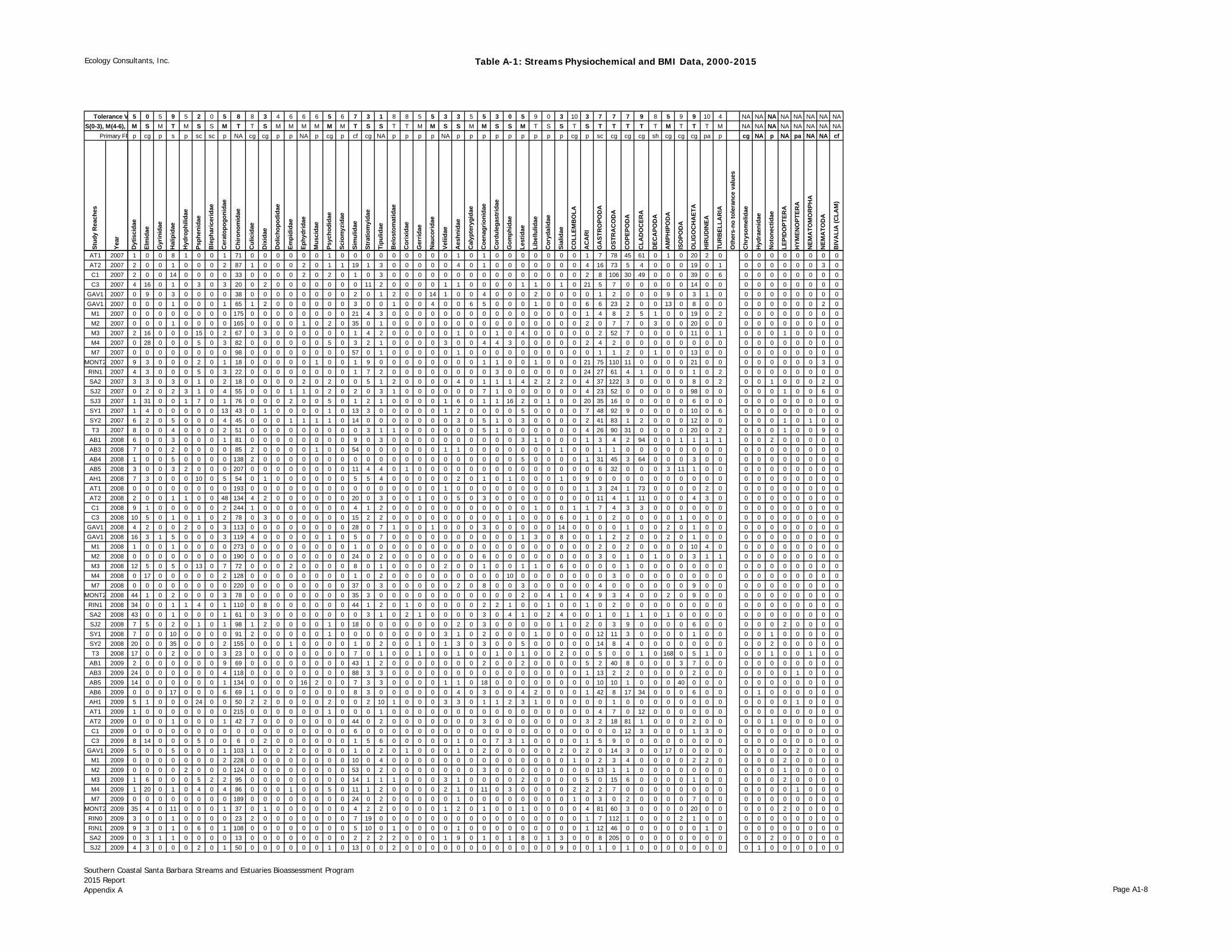
Ecology Consultants, Inc. Table A-1: Streams Physiochemical and BMI Data, 2000-2015
Southern Coastal Santa Barbara Streams and Estuaries Bioassessment Program2015 ReportAppendix A Page A1-8
Tolerance VS(0-3), M(4-6), T
Primary FF
Stud
y R
each
es
Year
AT1 2007AT2 2007C1 2007C3 2007
GAV1 2007GAV1 2007
M1 2007M2 2007M3 2007M4 2007M7 2007
MONT2 2007RIN1 2007SA2 2007SJ2 2007SJ3 2007SY1 2007SY2 2007T3 2007
AB1 2008AB3 2008AB4 2008AB5 2008AH1 2008AT1 2008AT2 2008C1 2008C3 2008
GAV1 2008GAV1 2008
M1 2008M2 2008M3 2008M4 2008M7 2008
MONT2 2008RIN1 2008SA2 2008SJ2 2008SY1 2008SY2 2008T3 2008
AB1 2009AB3 2009AB5 2009AB6 2009AH1 2009AT1 2009AT2 2009C1 2009C3 2009
GAV1 2009M1 2009M2 2009M3 2009M4 2009M7 2009
MONT2 2009RIN0 2009RIN1 2009SA2 2009SJ2 2009
5 0 5 9 5 2 0 5 8 8 3 4 6 6 6 5 6 7 3 1 8 8 5 5 3 3 5 5 3 0 5 9 0 3 10 3 7 7 7 9 8 5 9 9 10 4 NA NA NA NA NA NA NA NAM S M T M S S M T T S M M M M M M T S S T T M M S S M M S S M T S S T S T T T T T M T T T M NA NA NA NA NA NA NA NAp cg p s p sc sc p NA cg cg p p NA p cg p cf cg NA p p p p NA p p p p p p p p p cg p sc cg cg cg sh cg cg cg pa p cg NA p NA pa NA NA cf
Dyt
isci
dae
Elm
idae
Gyr
inid
ae
Hal
ipid
ae
Hyd
roph
ilida
e
Psph
enid
ae
Ble
phar
icer
idae
Cer
atop
ogon
idae
Chi
rono
mid
ae
Cul
icid
ae
Dix
idae
Dol
icho
podi
dae
Empi
dida
e
Ephy
drid
ae
Mus
cida
e
Psyc
hodi
dae
Scio
myz
idae
Sim
ulid
ae
Stra
tiom
yida
e
Tipu
lidae
Bel
osto
mat
idae
Cor
ixid
ae
Ger
ridae
Nau
corid
ae
Velii
dae
Aes
hnid
ae
Cal
ypte
rygi
dae
Coe
nagr
ioni
dae
Cor
dule
gast
ridae
Gom
phid
ae
Lest
idae
Libe
llulid
ae
Cor
ydal
idae
Sial
idae
CO
LLEM
BO
LA
AC
AR
I
GA
STR
OPO
DA
OST
RA
CO
DA
CO
PEPO
DA
CLA
DO
CER
A
DEC
APO
DA
AM
PHIP
OD
A
ISO
POD
A
OLI
GO
CH
AET
A
HIR
UD
INEA
TUR
BEL
LAR
IA
Oth
ers-
no to
lera
nce
valu
es
Chr
ysom
elid
ae
Hyd
raen
idae
Not
onec
tidae
LEPI
DO
PTER
A
HYM
ENO
PTER
A
NEM
ATO
MO
RPH
A
NEM
ATO
DA
BIV
ALI
A (C
LAM
)
1 0 0 8 1 0 0 1 71 0 0 0 0 0 0 1 0 0 0 0 0 0 0 0 0 1 0 1 0 0 0 0 0 0 0 1 7 78 45 61 0 1 0 20 2 0 0 0 0 0 0 0 0 02 0 0 1 0 0 0 2 87 1 0 0 0 2 0 1 1 19 1 3 0 0 0 0 0 4 0 1 0 0 0 0 0 0 0 4 16 73 5 4 0 0 0 19 0 1 0 0 0 0 0 0 3 02 0 0 14 0 0 0 0 33 0 0 0 0 2 0 2 0 1 0 3 0 0 0 0 0 0 0 0 0 0 0 0 0 0 0 2 8 106 30 49 0 0 0 39 0 6 0 0 0 0 0 0 0 04 16 0 1 0 3 0 3 20 0 2 0 0 0 0 0 0 0 11 2 0 0 0 0 1 1 0 0 0 0 1 1 0 1 0 21 5 7 0 0 0 0 0 14 0 0 0 0 0 0 0 0 0 00 9 0 3 0 0 0 0 38 0 0 0 0 0 0 0 0 2 0 1 2 0 0 14 1 0 0 4 0 0 0 2 0 0 0 0 1 2 0 0 0 9 0 3 1 0 0 0 0 0 0 0 0 00 0 0 1 0 0 0 1 65 1 2 0 0 0 0 0 0 3 0 0 1 0 0 4 0 0 6 5 0 0 0 1 0 0 0 6 6 23 2 0 0 13 0 8 0 0 0 0 0 0 0 0 2 00 0 0 0 0 0 0 0 175 0 0 0 0 0 0 0 0 21 4 3 0 0 0 0 0 0 0 0 0 0 0 0 0 0 0 1 4 8 2 5 1 0 0 19 0 2 0 0 0 0 0 0 0 00 0 0 1 0 0 0 0 165 0 0 0 0 1 0 2 0 35 0 1 0 0 0 0 0 0 0 0 0 0 0 0 0 0 0 2 0 7 7 0 3 0 0 20 0 0 0 0 0 0 0 0 0 02 16 0 0 0 15 0 2 67 0 3 0 0 0 0 0 0 1 4 2 0 0 0 0 0 1 0 0 1 0 4 0 0 0 0 0 2 52 7 0 0 0 0 11 0 1 0 0 0 1 0 0 0 00 28 0 0 0 5 0 3 82 0 0 0 0 0 0 5 0 3 2 1 0 0 0 0 3 0 0 4 4 3 0 0 0 0 0 2 4 2 0 0 0 0 0 0 0 0 0 0 0 0 0 0 0 00 0 0 0 0 0 0 0 98 0 0 0 0 0 0 0 0 57 0 1 0 0 0 0 0 1 0 0 0 0 0 0 0 0 0 0 1 1 2 0 1 0 0 13 0 0 0 0 0 0 0 0 0 09 3 0 0 0 2 0 1 18 0 0 0 0 0 1 0 0 1 9 0 0 0 0 0 0 0 0 1 1 0 0 1 0 0 0 21 75 110 11 0 0 0 0 21 0 0 0 0 0 0 0 0 3 04 3 0 0 0 5 0 3 22 0 0 0 0 0 0 0 0 1 7 2 0 0 0 0 0 0 0 0 3 0 0 0 0 0 0 24 27 61 4 1 0 0 0 1 0 2 0 0 0 0 0 0 0 03 3 0 3 0 1 0 2 18 0 0 0 0 2 0 2 0 0 5 1 2 0 0 0 0 4 0 1 1 1 4 2 2 2 0 4 37 122 3 0 0 0 0 8 0 2 0 0 1 0 0 0 2 00 2 0 2 3 1 0 4 55 0 0 0 1 1 0 2 0 2 0 3 1 0 0 0 0 0 0 7 1 0 0 0 0 0 0 4 23 52 0 0 0 0 0 98 0 0 0 0 0 1 0 0 6 01 31 0 0 1 7 0 1 76 0 0 0 2 0 0 5 0 1 2 1 0 0 0 0 1 6 0 1 1 16 2 0 1 0 0 20 35 16 0 0 0 0 0 6 0 0 0 0 0 0 0 0 0 01 4 0 0 0 0 0 13 43 0 1 0 0 0 0 1 0 13 3 0 0 0 0 0 1 2 0 0 0 0 5 0 0 0 0 7 48 92 9 0 0 0 0 10 0 6 0 0 0 0 0 0 0 06 2 0 5 0 0 0 4 45 0 0 0 1 1 1 1 0 14 0 0 0 0 0 0 0 3 0 5 1 0 3 0 0 0 0 2 41 83 1 2 0 0 0 12 0 0 0 0 0 1 0 1 0 08 0 0 4 0 0 0 2 51 0 0 0 0 0 0 0 0 0 3 1 1 0 0 0 0 0 0 5 1 0 0 0 0 0 0 4 26 90 31 0 0 0 0 20 0 2 0 0 0 1 0 0 9 06 0 0 3 0 0 0 1 81 0 0 0 0 0 0 0 0 9 0 3 0 0 0 0 0 0 0 0 0 0 3 1 0 0 0 1 3 4 2 94 0 0 1 1 1 1 0 0 2 0 0 0 0 07 0 0 2 0 0 0 0 85 2 0 0 0 0 1 0 0 54 0 0 0 0 0 0 1 1 0 0 0 0 0 0 0 1 0 0 1 1 0 0 0 0 0 0 0 0 0 0 0 0 0 0 0 01 0 0 5 0 0 0 0 138 2 0 0 0 0 0 0 0 0 0 0 0 0 0 0 0 0 0 0 0 0 5 0 0 0 0 1 31 45 3 64 0 0 0 3 0 0 0 0 0 0 0 0 0 03 0 0 3 2 0 0 0 207 0 0 0 0 0 0 0 0 11 4 4 0 1 0 0 0 0 0 0 0 0 0 0 0 0 0 0 6 32 0 0 0 3 11 1 0 0 0 0 0 0 0 0 0 07 3 0 0 0 10 0 5 54 0 1 0 0 0 0 0 0 5 5 4 0 0 0 0 0 2 0 1 0 1 0 0 0 1 0 9 0 0 0 0 0 0 0 0 0 0 0 0 0 0 0 0 0 00 0 0 0 0 0 0 0 193 0 0 0 0 0 0 0 0 0 0 0 0 0 0 0 1 0 0 0 0 0 0 0 0 0 0 1 3 24 1 73 0 0 0 0 2 0 0 0 0 0 0 0 0 02 0 0 1 1 0 0 48 134 4 2 0 0 0 0 0 0 20 0 3 0 0 1 0 0 5 0 3 0 0 0 0 0 0 0 0 11 4 1 11 0 0 0 4 3 0 0 0 0 0 0 0 0 09 1 0 0 0 0 0 2 244 1 0 0 0 0 0 0 0 4 1 2 0 0 0 0 0 0 0 0 0 0 0 1 0 0 1 1 7 4 3 3 0 0 0 0 0 0 0 0 0 0 0 0 0 010 5 0 1 0 1 0 2 78 0 3 0 0 0 0 0 0 15 2 2 0 0 0 0 0 0 0 0 0 1 0 0 0 6 0 1 0 2 0 0 0 0 1 0 0 0 0 0 0 0 0 0 0 04 2 0 0 2 0 0 3 113 0 0 0 0 0 0 0 0 28 0 7 1 0 0 1 0 0 0 3 0 0 0 0 0 14 0 0 0 0 1 0 0 2 0 1 0 0 0 0 0 0 0 0 0 016 3 1 5 0 0 0 3 119 4 0 0 0 0 0 1 0 5 0 7 0 0 0 0 0 0 0 0 0 0 1 3 0 8 0 0 1 2 2 0 0 2 0 1 0 0 0 0 0 0 0 0 0 01 0 0 1 0 0 0 0 273 0 0 0 0 0 0 0 0 1 0 0 0 0 0 0 0 0 0 0 0 0 0 0 0 0 0 0 2 0 2 0 0 0 0 10 4 0 0 0 0 0 0 0 0 00 0 0 0 0 0 0 0 190 0 0 0 0 0 0 0 0 24 0 2 0 0 0 0 0 0 0 6 0 0 0 0 0 0 0 0 3 0 1 0 1 0 0 3 1 1 0 0 0 0 0 0 0 012 5 0 5 0 13 0 7 72 0 0 0 2 0 0 0 0 8 0 1 0 0 0 0 2 0 0 1 0 0 1 1 0 6 0 0 0 0 1 0 0 0 0 0 0 0 0 0 0 0 0 0 0 00 17 0 0 0 0 0 2 128 0 0 0 0 0 0 0 0 1 0 2 0 0 0 0 0 0 0 0 0 10 0 0 0 0 0 0 0 3 0 0 0 0 0 0 0 0 0 0 0 0 0 0 0 00 0 0 0 0 0 0 0 220 0 0 0 0 0 0 0 0 37 0 3 0 0 0 0 0 2 0 8 0 0 3 0 0 0 0 0 4 0 0 0 0 0 0 9 0 0 0 0 0 0 0 0 0 044 1 0 2 0 0 0 3 78 0 0 0 0 0 0 0 0 35 3 0 0 0 0 0 0 0 0 0 0 0 2 0 4 1 0 4 9 3 4 0 0 2 0 9 0 0 0 0 0 0 0 0 0 034 0 0 1 1 4 0 1 110 0 8 0 0 0 0 0 0 44 1 2 0 1 0 0 0 0 0 2 2 1 0 0 1 0 0 1 0 2 0 0 0 0 0 0 0 0 0 0 0 0 0 0 0 043 0 0 1 0 0 0 1 61 0 3 0 0 0 0 0 0 0 3 1 0 2 1 0 0 0 0 3 0 4 1 0 2 4 0 0 1 0 1 1 0 1 0 0 0 0 0 0 0 0 0 0 0 07 5 0 2 0 1 0 1 98 1 2 0 0 0 0 1 0 18 0 0 0 0 0 0 0 2 0 3 0 0 0 0 0 1 0 2 0 3 9 0 0 0 0 6 0 0 0 0 0 2 0 0 0 07 0 0 10 0 0 0 0 91 2 0 0 0 0 0 1 0 0 0 0 0 0 0 0 3 1 0 2 0 0 0 1 0 0 0 0 12 11 3 0 0 0 0 1 0 0 0 0 1 0 0 0 0 020 0 0 35 0 0 0 2 155 0 0 0 1 0 0 0 0 1 0 2 0 0 1 0 1 3 0 3 0 0 5 0 0 0 0 0 14 8 4 0 0 0 0 0 0 0 0 0 2 0 0 0 0 017 0 0 2 0 0 0 3 23 0 0 0 0 0 0 0 0 7 0 1 0 0 1 0 0 1 0 0 1 0 1 0 0 2 0 0 5 0 0 1 0 168 0 5 1 0 0 0 1 0 0 1 0 02 0 0 0 0 0 0 9 69 0 0 0 0 0 0 0 0 43 1 2 0 0 0 0 0 0 0 2 0 0 2 0 0 0 0 5 2 40 8 0 0 0 3 7 0 0 0 0 0 0 0 0 0 024 0 0 0 0 0 0 4 118 0 0 0 0 0 0 0 0 88 3 3 0 0 0 0 0 0 0 0 0 0 0 0 0 0 0 1 13 2 2 0 0 0 0 2 0 0 0 0 0 0 1 0 0 014 0 0 0 0 0 0 1 134 0 0 0 0 16 2 0 0 7 3 3 0 0 0 0 1 1 0 18 0 0 0 0 0 0 0 0 10 10 1 0 0 0 40 0 0 0 0 0 0 0 0 0 0 00 0 0 17 0 0 0 6 69 1 0 0 0 0 0 0 0 8 3 0 0 0 0 0 0 4 0 3 0 0 4 2 0 0 0 1 42 8 17 34 0 0 0 6 0 0 0 1 0 0 0 0 0 05 1 0 0 0 24 0 0 50 2 2 0 0 0 0 2 0 0 2 10 1 0 0 0 3 3 0 1 1 2 3 1 0 0 0 0 0 1 0 0 0 0 0 0 0 0 0 0 0 0 1 0 0 01 0 0 0 0 0 0 0 215 0 0 0 0 0 0 1 0 0 0 1 0 0 0 0 0 0 0 0 0 0 0 0 0 0 0 0 4 7 0 12 0 0 0 0 0 0 0 0 0 0 0 0 0 00 0 0 1 0 0 0 1 42 7 0 0 0 0 0 0 0 44 0 2 0 0 0 0 0 0 0 3 0 0 0 0 0 0 0 3 2 18 81 1 0 0 0 2 0 0 0 0 1 0 0 0 0 00 0 0 0 0 0 0 0 0 0 0 0 0 0 0 0 0 6 0 0 0 0 0 0 0 0 0 0 0 0 0 0 0 0 0 0 0 0 12 3 0 0 0 1 3 0 0 0 0 0 0 0 0 08 14 0 0 0 5 0 0 6 0 2 0 0 0 0 0 0 1 5 6 0 0 0 0 0 1 0 0 7 3 1 0 0 0 0 1 5 9 0 0 0 0 0 0 0 0 0 0 0 0 0 0 0 05 0 0 5 0 0 0 1 103 1 0 0 2 0 0 0 0 1 0 2 0 1 0 0 0 1 0 2 0 0 0 0 0 2 0 2 0 14 3 0 0 17 0 0 0 0 0 0 0 0 2 0 0 00 0 0 0 0 0 0 2 228 0 0 0 0 0 0 0 0 10 0 4 0 0 0 0 0 0 0 0 0 0 0 0 0 0 1 0 2 3 4 0 0 0 0 2 2 0 0 0 0 2 0 0 0 00 0 0 0 2 0 0 0 124 0 0 0 0 0 0 0 0 53 0 2 0 0 0 0 0 0 0 3 0 0 0 0 0 0 0 0 13 1 1 0 0 0 0 0 0 0 0 0 0 1 0 0 0 01 6 0 0 0 5 2 2 95 0 0 0 0 0 0 0 0 14 1 1 1 0 0 0 3 1 0 0 0 0 2 0 0 0 0 5 0 15 6 0 0 0 0 1 0 0 0 0 0 2 0 0 0 01 20 0 1 0 4 0 4 86 0 0 0 1 0 0 5 0 11 1 2 0 0 0 0 2 1 0 11 0 3 0 0 0 0 2 2 2 7 0 0 0 0 0 0 0 0 0 0 0 0 1 0 0 00 0 0 0 0 0 0 0 189 0 0 0 0 0 0 0 0 24 0 2 0 0 0 0 0 1 0 0 0 0 0 0 0 0 1 0 3 0 2 0 0 0 0 7 0 0 0 0 0 0 0 0 0 035 4 0 11 0 0 0 1 37 0 1 0 0 0 0 0 0 4 2 2 0 0 0 0 1 2 0 1 0 0 1 0 0 0 0 4 81 60 3 0 0 0 0 20 0 0 0 0 0 2 0 0 0 03 0 0 1 0 0 0 0 23 2 0 0 0 0 0 0 0 7 19 0 0 0 0 0 0 0 0 0 0 0 0 0 0 0 0 1 7 112 1 0 0 0 2 1 0 0 0 0 0 0 0 0 0 09 3 0 1 0 6 0 1 108 0 0 0 0 0 0 0 0 5 10 0 1 0 0 0 0 1 0 0 0 0 0 0 0 0 0 1 12 46 0 0 0 0 0 0 1 0 0 0 0 0 0 0 0 00 3 1 1 0 0 0 0 13 0 0 0 0 0 0 0 0 2 2 2 2 0 0 0 1 9 0 1 0 1 8 0 1 3 0 0 8 205 0 0 0 0 0 0 0 0 0 0 2 0 0 0 0 04 3 0 0 0 2 0 1 50 0 0 0 0 0 0 1 0 13 0 0 2 0 0 0 0 0 0 0 0 0 0 0 0 9 0 0 1 0 1 0 0 0 0 0 0 0 0 1 0 0 0 0 0 0

Ecology Consultants, Inc. Table A-1: Streams Physiochemical and BMI Data, 2000-2015
Southern Coastal Santa Barbara Streams and Estuaries Bioassessment Program2015 ReportAppendix A Page A1-9
Tolerance VS(0-3), M(4-6), T
Primary FF
Stud
y R
each
es
Year
SJ3 2009SY1 2009SY2 2009T3 2009
AB1 2010AB2 2010AB3 2010AB5 2010AB7 2010AH1 2010AP1 2010AT1 2010AT2 2010C1 2010C3 2010
GAV1 2010M1 2010M2 2010M3 2010M4 2010
MONT2 2010RIN0 2010RIN1 2010SA2 2010SJ2 2010SJ3 2010SY1 2010SY2 2010T3 2010
AB1 2011AB3 2011AB5 2011AB7 2011AH1 2011C1 2011C3 2011
EC1 2011GAV1 2011
M1 2011M2 2011M3 2011M4 2011SJ2 2011SY1 2011SY2 2011AB1 2012AB3 2012AB5 2012AH1 2012C1 2012C3 2012
GAV1 2012M1 2012M3 2012M4 2012R0 2012SJ2 2012SY1 2012SY2 2012AB1 2013AB3 2013AB5 2013
5 0 5 9 5 2 0 5 8 8 3 4 6 6 6 5 6 7 3 1 8 8 5 5 3 3 5 5 3 0 5 9 0 3 10 3 7 7 7 9 8 5 9 9 10 4 NA NA NA NA NA NA NA NAM S M T M S S M T T S M M M M M M T S S T T M M S S M M S S M T S S T S T T T T T M T T T M NA NA NA NA NA NA NA NAp cg p s p sc sc p NA cg cg p p NA p cg p cf cg NA p p p p NA p p p p p p p p p cg p sc cg cg cg sh cg cg cg pa p cg NA p NA pa NA NA cf
Dyt
isci
dae
Elm
idae
Gyr
inid
ae
Hal
ipid
ae
Hyd
roph
ilida
e
Psph
enid
ae
Ble
phar
icer
idae
Cer
atop
ogon
idae
Chi
rono
mid
ae
Cul
icid
ae
Dix
idae
Dol
icho
podi
dae
Empi
dida
e
Ephy
drid
ae
Mus
cida
e
Psyc
hodi
dae
Scio
myz
idae
Sim
ulid
ae
Stra
tiom
yida
e
Tipu
lidae
Bel
osto
mat
idae
Cor
ixid
ae
Ger
ridae
Nau
corid
ae
Velii
dae
Aes
hnid
ae
Cal
ypte
rygi
dae
Coe
nagr
ioni
dae
Cor
dule
gast
ridae
Gom
phid
ae
Lest
idae
Libe
llulid
ae
Cor
ydal
idae
Sial
idae
CO
LLEM
BO
LA
AC
AR
I
GA
STR
OPO
DA
OST
RA
CO
DA
CO
PEPO
DA
CLA
DO
CER
A
DEC
APO
DA
AM
PHIP
OD
A
ISO
POD
A
OLI
GO
CH
AET
A
HIR
UD
INEA
TUR
BEL
LAR
IA
Oth
ers-
no to
lera
nce
valu
es
Chr
ysom
elid
ae
Hyd
raen
idae
Not
onec
tidae
LEPI
DO
PTER
A
HYM
ENO
PTER
A
NEM
ATO
MO
RPH
A
NEM
ATO
DA
BIV
ALI
A (C
LAM
)
3 7 0 0 0 7 0 0 37 0 1 0 0 0 0 0 0 2 4 0 0 0 0 0 1 14 0 9 0 11 4 0 0 0 0 2 8 11 0 0 0 0 0 0 0 0 0 0 0 0 0 0 0 02 0 0 0 0 0 0 4 121 0 0 0 0 5 0 1 0 61 0 0 0 0 0 0 0 0 0 0 0 0 0 0 0 0 0 0 0 0 1 0 0 0 0 15 0 0 0 0 0 4 0 0 0 04 0 0 0 1 0 0 4 85 0 0 0 0 4 0 0 0 36 5 0 0 0 0 0 0 0 0 0 0 0 1 0 0 0 0 2 0 1 0 0 0 0 0 2 0 0 0 0 0 8 0 0 0 033 0 0 0 0 0 0 3 210 5 0 0 0 0 0 0 0 0 0 0 0 0 0 0 0 3 0 0 0 0 12 0 0 0 0 3 0 0 0 0 0 0 0 4 0 0 0 0 0 0 0 0 0 01 0 0 3 0 0 0 0 90 0 0 0 0 4 0 0 0 80 0 1 0 0 0 0 0 0 0 5 0 0 1 1 0 0 0 1 0 6 0 0 0 0 4 6 1 0 0 0 0 0 0 0 0 05 0 0 2 0 0 0 0 113 0 0 0 0 6 0 1 0 93 0 1 0 0 1 0 0 0 0 0 0 0 5 0 0 0 0 0 0 0 2 0 0 0 0 0 1 0 0 0 0 0 1 0 0 01 0 0 1 0 0 0 0 33 0 0 0 0 0 1 0 0 146 2 0 0 0 0 0 0 0 0 0 0 0 0 0 0 0 0 1 0 0 0 0 0 0 0 0 0 0 0 0 0 0 0 0 0 02 0 0 1 0 0 0 0 206 0 0 0 0 0 0 0 0 36 2 0 0 0 0 0 0 1 0 1 0 0 0 0 0 0 0 0 0 12 3 0 0 4 15 5 0 0 0 0 1 0 0 0 0 00 0 0 2 0 0 0 0 176 0 0 0 0 0 0 0 0 48 2 2 0 0 0 0 0 0 0 8 0 0 1 1 0 0 1 1 6 20 5 0 0 0 0 4 0 0 0 0 0 0 0 0 0 02 4 0 0 0 21 0 4 74 0 1 0 0 0 0 0 0 3 0 8 0 0 0 0 1 1 0 1 0 0 0 0 0 1 0 2 0 0 0 0 0 0 0 0 0 0 0 0 0 0 0 0 0 116 0 0 10 0 0 0 1 53 0 0 0 2 0 1 1 0 110 0 3 0 0 1 0 0 0 0 1 0 0 0 0 0 0 0 0 41 4 0 0 0 0 0 1 0 0 0 0 0 0 0 0 0 02 0 0 0 1 0 0 0 78 0 0 0 0 0 0 0 0 0 0 0 0 0 0 0 0 0 0 0 0 0 0 0 0 0 0 0 2 8 3 198 0 0 0 7 0 0 0 0 0 0 0 0 0 00 0 0 0 0 0 0 0 77 0 0 0 1 0 0 0 0 117 1 0 0 0 0 0 0 0 0 1 0 0 0 0 0 0 0 0 1 1 2 0 0 0 0 26 0 0 0 0 0 0 1 0 0 00 0 0 0 0 0 0 0 136 0 0 0 0 1 0 0 0 5 0 1 0 0 0 0 0 0 0 0 0 0 0 0 0 0 0 0 120 7 10 1 0 0 0 13 0 5 0 0 0 0 0 0 0 014 3 0 0 0 2 0 1 54 0 0 0 0 0 0 1 0 14 0 0 0 0 0 0 1 0 0 1 1 0 0 0 0 7 0 0 1 5 0 0 0 0 0 6 0 0 0 0 0 0 0 0 0 23 0 0 0 0 0 0 1 96 0 0 0 1 0 0 0 0 1 0 1 0 1 0 1 0 0 0 3 0 0 0 0 0 19 0 0 0 0 7 4 0 0 0 2 0 0 0 0 0 0 0 0 0 10 1 0 3 0 0 0 0 189 0 0 0 0 3 0 2 0 55 1 0 0 0 0 0 0 0 0 1 0 0 0 0 0 0 0 1 0 1 0 0 0 0 0 1 0 0 0 0 0 0 0 0 0 00 0 0 0 0 0 0 0 138 0 0 0 1 0 0 0 0 85 0 1 0 0 0 0 0 0 0 5 0 0 0 0 0 0 0 0 3 1 3 0 0 0 0 1 0 0 0 0 0 0 0 0 0 00 4 0 0 0 3 0 0 129 0 0 0 0 0 0 1 0 48 0 0 0 0 0 0 1 0 0 0 0 0 3 0 0 2 0 0 0 0 0 0 0 0 0 0 0 0 0 0 0 0 1 0 0 04 2 0 1 0 0 4 0 164 0 0 0 2 0 0 3 0 32 0 0 0 0 0 0 0 0 0 0 0 2 0 0 0 0 0 1 0 0 0 0 0 0 0 0 0 0 0 0 0 0 0 0 0 04 2 0 1 0 1 0 0 125 10 0 0 0 0 0 0 0 35 2 1 1 0 0 0 0 0 0 0 0 0 0 0 0 4 0 2 0 1 2 0 0 0 0 9 0 0 0 0 0 0 0 0 0 18 0 0 1 0 0 0 0 49 0 0 0 0 0 0 0 0 58 0 0 0 0 0 0 0 0 0 1 0 0 0 0 0 1 0 0 1 2 0 0 0 0 0 0 0 0 0 0 0 0 0 0 0 06 0 1 1 0 1 0 2 91 0 2 0 0 1 0 0 0 1 0 0 3 0 0 0 0 0 0 1 1 1 0 0 0 0 0 0 4 2 1 0 0 0 0 1 0 0 0 0 1 0 0 0 0 05 0 0 2 0 0 0 4 98 0 0 0 0 0 1 0 0 12 1 1 2 0 0 0 3 0 0 0 1 1 0 0 0 0 0 1 1 0 0 0 0 0 0 3 0 0 0 0 0 0 0 0 0 06 1 0 3 0 0 0 66 129 0 0 0 2 1 2 0 0 29 0 1 1 0 0 0 0 0 0 2 0 1 0 0 0 0 0 0 1 0 3 0 0 0 0 1 0 0 0 0 0 0 0 0 0 02 13 0 0 0 4 0 0 104 0 1 0 0 0 0 0 0 1 0 2 0 0 0 0 2 2 0 2 1 12 1 0 0 3 0 4 6 0 0 0 0 0 1 11 0 0 0 0 0 0 0 0 0 03 0 0 2 0 0 0 0 108 0 0 0 0 0 0 2 0 41 0 2 0 0 0 0 0 0 0 0 0 0 0 0 0 0 0 0 0 1 4 0 0 0 0 4 0 0 0 0 0 0 0 0 0 04 0 0 2 0 0 0 1 96 0 0 0 0 0 0 0 0 60 0 0 0 0 0 0 0 0 0 2 0 0 0 0 0 0 0 0 0 0 2 0 0 0 0 0 0 0 0 0 1 0 0 0 0 05 0 0 0 0 0 0 0 61 0 0 0 1 0 0 0 0 4 0 1 0 0 0 0 0 0 0 0 0 0 0 0 0 0 0 1 0 0 0 0 0 0 0 13 0 0 0 0 0 0 0 0 0 08 0 0 4 0 0 0 1 65 0 0 0 0 0 0 0 0 1 0 1 0 0 0 0 0 0 0 2 1 0 0 0 0 0 0 0 0 4 3 0 0 0 110 17 0 0 0 0 0 1 0 0 0 06 1 0 1 1 0 0 1 82 0 0 0 0 0 0 0 0 29 0 0 0 0 0 0 0 0 0 0 0 0 0 0 0 0 0 1 2 0 0 0 0 0 0 0 0 0 0 0 0 0 0 0 0 029 0 0 0 0 0 0 0 171 0 0 0 2 1 2 1 0 16 0 4 0 0 1 0 0 1 0 0 0 0 0 0 0 0 0 1 7 10 4 0 0 1 46 2 0 0 0 0 0 0 0 0 0 00 0 0 0 0 0 0 0 84 0 0 0 3 0 0 0 0 4 3 1 0 0 0 0 0 0 0 14 0 0 0 0 0 0 0 0 9 3 4 0 0 2 0 4 13 0 0 0 1 0 0 0 0 02 0 0 0 0 3 0 5 41 0 1 0 0 0 0 0 0 13 2 6 0 0 0 0 1 0 0 1 0 1 1 0 0 2 0 0 0 0 0 0 0 0 0 0 0 0 0 0 0 0 1 0 0 00 0 0 0 0 0 0 2 173 0 2 0 0 0 0 0 0 34 0 0 0 0 0 0 0 0 0 0 0 0 0 0 0 0 2 1 0 0 3 0 0 0 0 17 0 0 0 0 0 0 0 0 0 05 3 0 0 0 1 0 2 10 0 3 0 0 0 0 0 0 0 5 0 0 0 1 0 1 0 0 0 0 0 0 0 0 1 0 1 0 0 0 0 0 0 0 2 0 0 0 0 0 0 0 1 0 09 0 0 1 0 0 0 0 104 0 0 0 0 0 0 0 0 0 1 1 0 2 0 0 0 0 0 0 0 0 1 0 0 1 0 0 1 0 1 0 0 0 3 7 0 0 0 0 0 0 0 0 0 01 0 0 0 0 0 0 5 161 0 0 0 0 1 1 0 0 3 0 0 0 0 0 0 0 0 0 2 0 0 0 0 0 4 0 1 0 1 0 0 0 2 0 0 0 0 0 0 0 0 0 0 0 01 0 1 0 0 0 0 1 156 0 0 0 0 1 0 1 0 26 0 0 0 0 0 0 0 0 0 0 0 0 0 0 0 0 0 0 0 8 1 0 0 0 0 0 0 0 0 0 0 0 0 0 0 01 0 0 0 1 0 0 0 111 0 0 0 0 0 0 0 0 46 0 8 0 0 0 0 0 0 0 5 0 0 0 0 0 0 0 0 5 0 0 0 0 0 0 4 0 0 0 0 0 0 0 0 0 05 6 0 0 0 2 1 1 93 0 0 0 0 0 0 1 0 22 0 0 0 0 0 0 0 0 0 1 1 0 0 0 0 0 0 1 0 0 0 0 0 0 0 0 0 0 0 0 0 0 0 1 0 01 4 0 0 0 0 2 1 97 0 0 0 0 0 0 0 0 2 0 2 0 0 0 0 0 0 0 0 0 0 1 0 1 0 0 3 0 0 0 0 0 0 0 0 0 0 0 0 0 0 0 0 0 07 4 0 0 0 0 0 4 187 0 0 0 0 0 0 1 0 25 0 0 1 0 0 0 1 0 0 1 0 0 0 0 0 1 0 0 0 1 1 0 0 0 0 0 0 0 0 0 0 0 0 0 0 024 0 0 1 0 0 0 1 104 0 0 0 1 0 0 6 0 8 0 0 0 0 0 0 0 0 0 0 0 0 0 0 0 0 0 1 0 0 2 0 0 0 0 0 0 0 0 0 0 0 0 0 0 018 0 0 1 0 0 0 2 60 0 0 0 0 0 0 0 0 3 0 2 0 0 1 0 0 0 0 0 0 0 2 0 0 0 0 0 2 0 0 0 0 0 1 2 0 0 0 0 0 0 0 0 0 00 0 0 0 0 0 0 0 30 0 0 0 1 0 0 0 0 4 4 0 0 0 0 0 0 1 0 0 0 0 1 0 0 0 0 2 0 0 5 0 0 0 179 2 0 0 0 0 0 0 0 1 0 06 2 0 1 0 0 0 1 22 0 0 0 0 0 0 2 0 4 93 0 0 0 0 0 0 0 0 0 0 0 0 0 0 0 0 1 32 60 0 0 0 1 1 2 0 1 0 0 0 1 0 0 0 08 0 0 3 0 0 0 0 82 0 0 0 2 1 0 0 0 6 0 1 0 0 0 0 2 0 0 9 0 0 0 0 0 0 7 0 7 3 0 0 0 74 57 19 0 3 0 0 0 0 0 0 0 00 4 0 0 0 5 0 4 63 0 0 0 0 0 0 1 0 0 2 5 0 0 0 0 0 0 0 0 1 0 0 0 0 0 0 2 2 0 0 0 0 0 0 1 0 0 0 0 0 0 0 0 0 10 0 0 2 0 0 0 0 33 0 0 0 0 0 1 0 0 1 1 1 0 0 0 0 0 0 0 1 0 0 0 0 0 0 0 0 46 11 4 106 0 0 0 89 0 0 0 0 0 0 0 0 0 43 11 0 0 0 0 0 1 102 0 0 0 0 0 0 0 0 0 8 1 0 0 1 0 0 0 0 1 1 0 0 0 0 0 0 0 0 0 0 0 0 0 0 3 0 0 0 0 0 0 0 1 0 42 1 0 0 0 0 0 1 6 0 0 0 0 0 0 0 0 0 1 1 0 0 0 0 0 0 0 2 1 0 0 0 0 0 0 1 1 8 0 0 0 11 0 0 0 0 0 0 0 0 0 0 0 10 0 0 1 0 0 0 1 87 0 0 0 0 0 1 1 0 5 3 0 0 0 0 0 0 0 0 0 0 0 0 0 0 0 0 1 1 0 1 0 0 0 0 16 0 0 0 0 0 0 1 0 0 02 12 0 0 0 8 1 4 40 0 0 0 0 0 0 0 0 20 5 0 0 0 1 0 1 0 0 1 0 0 2 0 0 0 0 7 3 5 12 0 0 0 0 6 0 2 0 0 0 0 0 0 0 02 8 0 0 0 2 0 0 96 0 0 0 0 0 0 1 0 0 0 0 0 0 2 0 0 2 0 0 1 0 0 0 0 0 0 0 5 13 0 0 0 0 0 2 0 3 0 0 0 0 0 1 0 02 1 0 0 0 2 0 3 76 0 2 0 1 0 0 4 0 12 0 3 0 0 0 0 1 0 0 1 0 0 0 0 0 0 0 2 5 1 0 0 0 0 1 1 0 0 0 0 1 0 0 0 0 02 16 0 0 0 0 0 2 23 0 0 0 0 0 0 1 0 1 2 0 0 0 0 0 0 0 0 0 0 2 0 0 0 3 0 2 20 7 2 0 0 0 0 8 0 2 0 0 0 0 0 0 0 01 4 0 2 0 0 0 6 101 0 0 0 0 0 0 0 0 15 0 1 0 0 0 0 0 0 0 0 0 0 2 0 0 0 0 7 25 2 5 0 0 0 0 18 0 6 0 0 0 0 0 0 0 04 1 0 1 0 1 0 5 106 0 0 0 1 0 0 0 0 26 2 0 1 0 0 0 0 0 0 4 0 0 0 0 0 0 0 1 3 3 1 0 0 0 0 13 0 2 0 0 0 0 0 0 0 07 0 0 1 0 0 0 2 95 0 0 0 0 0 0 0 0 35 0 1 0 0 0 0 0 2 0 3 0 0 0 0 0 0 0 0 1 1 0 0 0 1 94 1 0 2 0 0 0 1 0 0 0 08 1 0 0 0 0 0 0 146 0 1 0 0 0 0 1 0 0 0 2 0 0 1 0 0 0 0 0 0 0 4 0 0 0 0 0 24 84 0 3 0 0 0 14 0 4 0 0 0 0 0 0 0 07 0 0 4 1 0 0 1 94 0 0 0 2 0 0 1 0 9 0 1 0 0 0 0 0 0 0 4 0 0 0 0 0 0 0 0 39 12 12 0 0 2 29 5 0 0 0 0 0 0 0 0 0 0

Ecology Consultants, Inc. Table A-1: Streams Physiochemical and BMI Data, 2000-2015
Southern Coastal Santa Barbara Streams and Estuaries Bioassessment Program2015 ReportAppendix A Page A1-10
Tolerance VS(0-3), M(4-6), T
Primary FF
Stud
y R
each
es
Year
AH1 2013C1 2013C3 2013
GAV1 2013M1 2013M2 2013M3 2013M4 2013SA2 2013SJ2 2013SY1 2013SY2 2013AB1 2014AB3 2014AB5 2014AH1 2014C1 2014C3 2014
GAV1 2014M1 2014M2 2014M3 2014M4 2014SJ2 2014SY2 2014AB1 2015AB5 2015AB7 2015AB8 2015AH0 2015AH1 2015C1 2015C3 2015
GAV1 2015LC1 2015M1 2015M2 2015M3 2015M4 2015SJ2 2015SY2 2015
5 0 5 9 5 2 0 5 8 8 3 4 6 6 6 5 6 7 3 1 8 8 5 5 3 3 5 5 3 0 5 9 0 3 10 3 7 7 7 9 8 5 9 9 10 4 NA NA NA NA NA NA NA NAM S M T M S S M T T S M M M M M M T S S T T M M S S M M S S M T S S T S T T T T T M T T T M NA NA NA NA NA NA NA NAp cg p s p sc sc p NA cg cg p p NA p cg p cf cg NA p p p p NA p p p p p p p p p cg p sc cg cg cg sh cg cg cg pa p cg NA p NA pa NA NA cf
Dyt
isci
dae
Elm
idae
Gyr
inid
ae
Hal
ipid
ae
Hyd
roph
ilida
e
Psph
enid
ae
Ble
phar
icer
idae
Cer
atop
ogon
idae
Chi
rono
mid
ae
Cul
icid
ae
Dix
idae
Dol
icho
podi
dae
Empi
dida
e
Ephy
drid
ae
Mus
cida
e
Psyc
hodi
dae
Scio
myz
idae
Sim
ulid
ae
Stra
tiom
yida
e
Tipu
lidae
Bel
osto
mat
idae
Cor
ixid
ae
Ger
ridae
Nau
corid
ae
Velii
dae
Aes
hnid
ae
Cal
ypte
rygi
dae
Coe
nagr
ioni
dae
Cor
dule
gast
ridae
Gom
phid
ae
Lest
idae
Libe
llulid
ae
Cor
ydal
idae
Sial
idae
CO
LLEM
BO
LA
AC
AR
I
GA
STR
OPO
DA
OST
RA
CO
DA
CO
PEPO
DA
CLA
DO
CER
A
DEC
APO
DA
AM
PHIP
OD
A
ISO
POD
A
OLI
GO
CH
AET
A
HIR
UD
INEA
TUR
BEL
LAR
IA
Oth
ers-
no to
lera
nce
valu
es
Chr
ysom
elid
ae
Hyd
raen
idae
Not
onec
tidae
LEPI
DO
PTER
A
HYM
ENO
PTER
A
NEM
ATO
MO
RPH
A
NEM
ATO
DA
BIV
ALI
A (C
LAM
)
1 3 0 0 0 15 0 4 81 0 5 0 0 0 0 9 0 1 1 8 0 0 0 0 14 1 0 1 1 0 0 0 0 2 0 2 5 0 1 0 0 0 2 0 0 0 1 0 0 0 0 0 0 10 0 0 0 0 0 0 0 35 0 0 0 0 0 0 0 0 0 0 3 0 0 0 0 0 0 0 0 0 0 0 0 0 0 0 0 25 4 0 13 0 0 0 75 0 1 0 0 0 0 0 0 0 64 5 0 0 0 0 0 3 135 1 0 0 1 0 0 1 0 18 0 0 1 0 0 0 2 2 0 1 0 0 1 0 0 0 0 0 4 0 0 0 0 0 1 0 0 1 0 0 0 0 0 0 0 30 0 0 0 0 0 0 5 72 0 1 0 0 0 0 0 0 0 0 0 0 6 0 0 0 0 0 5 0 0 1 0 0 10 0 0 0 19 3 0 0 10 0 2 0 6 0 0 0 0 0 0 0 50 0 0 1 0 0 0 0 240 0 0 0 0 0 0 0 0 19 0 0 0 0 0 0 0 0 0 0 0 0 0 0 0 0 0 0 0 0 0 13 0 2 0 13 0 12 0 0 0 0 0 0 0 00 0 0 0 0 0 0 0 103 0 0 0 0 0 0 0 0 0 0 12 0 0 0 0 0 0 0 20 0 0 0 0 0 0 0 0 140 2 4 0 1 0 0 9 0 0 0 0 0 1 0 0 0 01 17 0 0 0 1 0 9 79 0 0 0 0 0 0 3 0 0 0 0 0 0 0 0 0 0 0 1 0 0 2 0 0 0 0 0 7 106 0 0 0 0 0 16 0 12 0 0 0 0 0 0 0 10 7 0 1 0 1 0 6 142 0 0 0 1 0 0 1 0 4 0 2 0 0 1 0 0 2 0 1 0 0 7 0 0 0 0 0 4 20 0 0 0 0 0 0 0 1 0 0 4 0 0 0 0 05 0 0 0 0 2 0 1 57 1 5 0 0 0 0 0 0 0 0 1 0 0 0 0 0 0 0 0 0 0 16 0 0 1 0 0 38 18 1 0 0 0 0 3 0 0 0 0 0 1 0 0 0 00 7 0 0 0 0 0 4 52 0 1 0 0 0 0 1 0 0 0 2 1 0 0 0 0 0 0 1 0 0 0 0 0 0 0 0 3 29 0 0 0 0 0 11 0 0 0 0 0 0 0 0 0 05 2 0 4 0 0 0 0 18 0 0 0 0 0 0 0 0 1 0 0 0 0 0 0 1 0 0 0 0 0 0 0 0 0 0 4 186 22 24 0 0 0 0 1 0 12 0 0 0 0 0 0 0 00 5 0 2 0 0 0 4 152 0 1 0 0 0 0 0 0 7 1 3 0 0 1 0 0 0 0 14 0 0 3 0 0 3 0 0 18 11 1 0 0 0 0 12 0 5 0 0 0 0 0 0 0 01 0 0 1 0 0 0 0 142 0 0 0 0 0 0 0 0 10 0 1 0 0 0 0 0 0 0 1 0 0 0 0 0 1 0 1 10 1 2 0 0 0 27 4 0 1 0 0 0 0 0 1 0 37 0 0 0 1 0 0 2 67 1 0 0 0 0 0 0 0 75 0 1 0 0 1 0 0 0 0 0 0 0 0 0 1 0 0 3 3 9 0 1 0 0 0 4 0 0 0 0 0 0 0 0 0 08 0 0 0 0 0 0 0 80 0 0 0 0 0 0 0 0 2 0 0 0 0 0 0 0 0 0 1 0 0 0 0 0 0 0 0 30 65 24 3 0 34 2 4 0 1 0 0 0 0 0 0 0 03 4 0 0 0 5 0 2 135 0 2 0 2 0 0 0 0 22 0 0 0 0 0 0 0 0 0 5 0 0 0 0 0 0 0 1 2 0 1 0 0 0 0 0 0 0 0 0 0 0 0 0 0 00 0 0 3 0 0 0 0 40 1 0 0 0 0 1 0 0 2 0 0 0 0 0 0 0 0 0 5 0 0 0 0 0 0 0 4 51 108 5 7 0 0 0 9 0 1 0 0 0 0 0 0 0 45 2 0 0 0 0 1 0 93 0 0 0 1 0 0 0 0 122 0 1 0 0 0 0 0 0 0 0 0 0 0 0 0 0 0 0 0 2 0 0 0 0 1 5 0 0 0 0 0 0 0 0 0 2
10 0 0 0 0 1 0 0 134 2 0 0 1 0 0 1 0 0 0 1 0 0 0 0 0 0 0 0 0 0 0 0 0 0 0 5 12 2 7 0 0 14 0 1 0 0 0 0 0 0 0 0 0 00 0 0 0 0 0 0 0 102 0 0 0 1 0 0 0 0 7 0 0 0 0 0 0 0 0 0 0 0 0 0 0 0 0 0 0 0 5 11 0 0 2 0 22 0 8 0 0 0 0 0 0 0 10 0 0 0 0 0 0 0 232 0 0 0 4 0 0 0 0 11 0 0 0 0 0 0 0 0 0 15 0 0 0 0 0 0 0 0 27 2 3 0 1 0 0 5 0 0 0 0 0 0 0 0 0 06 5 0 0 0 2 0 0 131 0 0 0 3 0 0 1 0 28 1 0 1 0 0 0 0 0 0 2 0 0 8 0 0 0 0 1 7 32 16 0 0 0 0 4 3 0 0 0 1 0 0 0 0 104 4 0 1 0 1 0 3 71 0 0 0 2 0 0 0 0 61 0 1 2 0 0 0 0 1 0 6 0 0 3 0 0 0 1 2 6 70 4 0 0 0 0 6 0 4 0 0 0 0 1 0 0 00 1 0 0 0 0 0 4 140 26 0 0 1 0 0 1 0 50 2 1 1 0 0 0 0 0 0 7 0 0 0 0 0 0 0 1 1 1 1 0 0 0 0 5 0 0 0 0 0 2 0 0 0 00 3 0 0 0 1 0 8 135 0 0 0 2 0 0 0 0 42 0 0 0 0 0 0 0 1 0 22 0 0 0 0 0 0 0 1 8 15 5 0 0 0 0 3 0 1 0 0 0 0 0 0 0 03 0 0 2 0 0 0 1 116 0 0 0 0 0 0 0 0 56 0 2 0 0 0 0 0 0 0 6 0 0 0 0 0 0 0 1 1 5 0 1 0 40 14 1 0 5 0 0 0 0 0 0 0 11 0 0 1 0 0 0 0 67 4 0 0 0 1 0 0 0 1 0 1 0 0 2 0 0 1 0 0 0 0 1 0 0 0 0 1 31 83 7 0 0 0 38 4 0 0 0 0 6 2 1 0 0 00 0 0 5 0 0 0 0 101 0 0 0 0 0 0 0 0 20 5 0 0 0 0 0 1 0 0 7 0 0 3 1 0 0 0 1 17 6 19 0 0 12 0 14 0 66 0 0 0 0 0 0 0 100 0 0 2 0 0 0 0 60 1 0 0 0 0 0 0 0 0 2 0 0 0 0 0 2 2 0 0 0 0 3 0 0 0 0 0 38 71 14 0 0 0 0 47 1 41 0 0 0 0 0 0 0 170 0 0 0 0 0 0 2 244 17 0 0 0 0 0 0 0 0 0 2 0 0 0 0 0 0 0 0 0 0 0 0 0 0 0 0 2 14 0 0 0 0 0 0 0 4 0 0 0 0 0 0 0 01 3 0 0 0 3 0 1 74 0 0 0 2 0 0 0 0 17 1 6 1 0 0 0 0 2 0 6 0 0 0 0 0 0 0 1 3 1 1 0 0 0 0 0 0 0 0 0 0 0 0 0 0 60 0 0 2 0 0 0 3 51 0 0 0 0 0 0 0 0 0 0 1 0 0 0 0 0 0 0 2 0 0 0 0 0 0 0 0 2 23 3 0 0 0 0 22 0 0 0 0 0 0 0 0 0 510 0 0 2 1 0 0 0 185 2 1 0 0 0 0 0 0 30 0 0 0 0 0 0 1 0 0 0 0 0 1 0 0 0 0 0 7 0 2 0 0 0 0 0 0 0 0 0 0 0 0 0 0 09 1 2 0 1 0 0 1 210 0 3 0 0 0 2 0 0 0 0 1 0 0 1 0 0 0 0 0 0 0 0 1 0 0 0 3 10 3 4 0 0 0 0 0 0 0 0 0 0 0 0 0 0 00 2 0 0 0 1 0 1 64 0 0 0 0 0 0 0 0 9 2 1 1 0 0 0 2 6 0 2 0 0 6 0 0 2 0 3 92 3 1 0 0 0 0 0 0 4 0 0 0 0 0 0 0 400 0 0 0 0 0 0 0 56 67 0 0 0 0 0 0 0 0 0 0 0 0 0 0 0 0 0 0 0 0 0 0 0 0 0 0 0 0 11 158 0 2 0 0 0 3 0 0 0 0 1 0 0 20 0 0 0 0 0 0 0 57 0 0 0 0 0 0 0 0 146 0 6 0 0 1 0 0 0 0 4 0 0 0 0 0 0 0 0 53 1 0 0 1 11 0 4 0 4 0 0 0 0 0 0 0 01 1 0 2 0 1 0 0 88 5 1 0 0 0 0 0 0 5 0 1 0 0 0 0 3 6 0 12 0 0 3 0 0 0 0 1 24 77 5 1 0 13 0 6 0 0 0 0 0 0 1 0 0 60 0 0 1 0 0 0 0 42 2 0 0 0 0 0 0 0 0 0 0 0 0 0 0 0 0 0 0 0 0 0 0 0 0 0 0 27 19 8 0 0 0 0 2 0 0 0 0 1 0 1 0 0 010 2 0 2 0 1 0 4 132 0 0 0 3 1 0 0 0 2 0 6 2 0 0 0 0 0 0 28 0 0 0 0 0 3 0 1 4 10 0 0 1 0 0 7 0 0 0 0 0 0 0 0 0 05 3 0 2 0 1 0 4 132 0 0 0 0 0 0 0 0 39 0 0 1 0 0 0 0 1 0 6 0 0 0 0 0 2 0 3 9 29 12 0 0 11 0 13 0 0 0 0 0 0 0 0 0 0
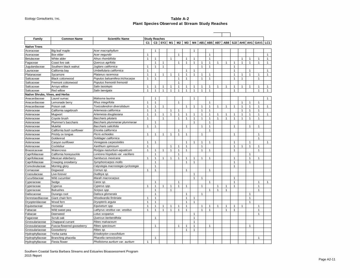
Ecology Consultants, Inc. Table A-2Plant Species Observed at Stream Study Reaches
Southern Coastal Santa Barbara Streams and Estuaries Bioassessment Program2015 Report
Page A2-11
Family Common Name Scientific NameC1 C3 SY2 M1 M2 M3 M4 AB1 AB5 AB7 AB8 SJ2 AH0 AH1 GAV1 LC1
Native TreesAceraceae Big-leaf maple Acer macrophyllum 1 1Aceraceae Box elder Acer negundo 1 1 1 1Betulaceae White alder Alnus rhombifolia 1 1 1 1 1 1 1 1 1 1Fagaceae Coast live oak Quercus agrifolia 1 1 1 1 1 1 1 1 1 1 1 1 1 1Jugulandaceae Southern black walnut Juglans californica 1 1 1 1 1 1Lauraceae California bay Umbellularia californica 1 1 1 1 1 1Platanaceae Sycamore Platanus racemosa 1 1 1 1 1 1 1 1 1 1 1 1 1 1Salicaceae Black cottonwood Populus balsamifera trichocarpa 1 1 1 1 1 1 1 1 1Salicaceae Fremont cottonwood Populus fremontii fremontii 1Salicaceae Arroyo willow Salix lasiolepis 1 1 1 1 1 1 1 1 1 1 1 1 1 1 1 1Salicaceae Red willow Salix laevigata 1 1 1 1 1 1 1 1 1 1 1 1Native Shrubs, Vines, and HerbsAnacardiaceae Laurel sumac Malosma laurina 1 1 1Anacardiaceae Lemonade berry Rhus integrifolia 1 1 1 1 1 1 1Anacardiaceae Poison oak Toxicodendron diversilobum 1 1 1 1 1 1 1 1 1 1 1 1 1 1Asteraceae California sagebrush Artemesia californica 1 1 1 1 1 1 1 1 1Asteraceae Mugwort Artemesia douglasiana 1 1 1 1 1 1 1 1 1 1 1 1 1 1 1 1Asteraceae Coyote brush Baccharis pilularis 1 1 1 1 1 1 1 1 1 1 1 1 1Asteraceae Plummer's baccharis Baccharis plummerae plummerae 1 1 1Asteraceae Mulefat Baccharis salicifolia 1 1 1 1 1 1 1 1Asteraceae California bush sunflower Encelia californica 1 1Asteraceae Prickly ox tongue Picris echioides 1 1 1 1 1 1 1 1 1Asteraceae Goldenrod Solidager californica 1Asteraceae Canyon sunflower Venegasia carpesioides 1 1 1 1 1 1 1 1 1Asteraceae Cocklebur Xanthium spinosum 1 1 1 1 1 1 1 1 1Brassicaceae Watercress Rorippa nasturtium-aquaticum 1 1 1 1 1 1 1 1 1 1Caprifoliaceae California honeysuckle Lonicera hispidula var. vacillans 1 1 1Caprifoliaceae Mexican elderberry Sambucus mexicana 1 1 1 1 1 1 1 1 1 1 1 1Caprifoliaceae Creeping snowberry Symphoricarpos mollis 1 1 1 1 1Convolvulaceae Morning glory Calystegia macrostegia cyclostegia 1 1Cornaceae Dogwood Cornus sp. 1 1 1 1Crassulaceae Live-forever Dudleya sp. 1Cucurbitaceae Wild cucumber Marah macrocarpus 1 1 1Cyperaceae Sedge Carex sp. 1 1 1 1 1 1Cyperaceae Cyperus Cyperus spp. 1 1 1 1 1 1 1 1 1 1 1Cyperaceae Bulrushes Scirpus spp. 1 1 1 1 1 1Datiscaceae Durango root Datisca glomerata 1 1 1 1Dennstaedtiaceae Giant chain fern Woodwardia fimbriata 1 1 1 1 1Dryopteridaceae Wood fern Dryopteris arguta 1 1 1 1 1Equisetaceae Horsetail Equisetum spp. 1 1 1 1 1 1 1 1 1 1 1 1 1Fabacae Wild sweet pea Lathyrus vestitus var. vestitus 1 1 1 1 1 1 1 1 1 1 1Fabacae Deerweed Lotus scoparius 1 1Fagaceae Scrub oak Quercus berberdifolia 1 1Grossulariaceae Chapparal currant Ribes malvaceum 1Grossulariaceae Fuscia-flowered gooseberry Ribes speciosum 1 1 1 1 1 1Grossulariaceae Gooseberry Ribes sp. 1 1Hydrophyllaceae Yerba santa Eriodictylon crassifoliumHydrophyllaceae Branching phacelia Phacelia ramosissima 1 1Hydrophyllaceae Fiesta flower Pholistoma auritum var. auritum 1
Study Reaches

Ecology Consultants, Inc. Table A-2Plant Species Observed at Stream Study Reaches
Southern Coastal Santa Barbara Streams and Estuaries Bioassessment Program2015 Report
Page A2-12
Family Common Name Scientific NameC1 C3 SY2 M1 M2 M3 M4 AB1 AB5 AB7 AB8 SJ2 AH0 AH1 GAV1 LC1
Study Reaches
Juncaceae Rushes Juncus spp. 1 1 1 1 1 1Lamiaceae Purple sage Salvia leucophylla 1Lamiaceae Black sage Salvia mellifera 1 1 1Lamiaceae Crimson pitcher sage Salvia spathacea 1 1 1Lamiaceae Wood mint, hedge nettle Stachys bullata 1 1 1 1 1Liliaceae Humboldt lily Lilium humboldtii humboldtii 1 1Onagraceae Willow herb Epilobium ciliatum 1 1 1 1 1 1Onagraceae California fuschia Epilobium canum ssp. canumOnagraceae Hooker's evening primrose Oenothera elata ssp. hirsutissmaOrchidaceae Stream orchid Epipactis gigantea 1Oxalidaceae Oxalis Oxalis albicansPapaveraceae California poppy Eschscholzia californica 1Papaveraceae Bush poppy Dendromecon rigidaPoaceae Giant ryegrass Elymus condensatus 1 1 1 1 1 1 1 1Polygonaceae Ashyleaf buckwheat Eriogonum cinereum 1Polygonaceae California buckwheat Eriogonum fasciculatum 1Polygonaceae Water smartweed Polygonum amphibium var. emersum 1 1 1 1 1 1 1 1Polypodiaceae California polypody Polypodium californicum 1Potamogetonaceae Pondweeds Potamogeton spp. 1 1 1 1 1 1 1Pteridaceae Venus-hair fern Adiantum capillus-verneris 1 1 1Ranunculaceae Virgin's bower Clematis ligustifolia 1 1 1 1 1 1 1 1 1Ranunculaceae Meadow rue Thalictrum fendlerli var. polycarpum 1 1 1Rhamnaceae Buck brush Ceanothus cuneatus 1 1 1Rhamnaceae Hairy-leaved ceanothus Ceanothus oliganthusRhamnaceae Big pod ceanothus Ceanothus megacarpusRhamnaceae Greenbark ceanothus Ceanothus spinosus 1 1Rhamnaceae Coffee berry Rhamnus californica 1 1 1 1Rhamnaceae Redberry Rhamnus crocea 1Rhamnaceae Hollyleaf redberry Rhamnus ilicifoliaRosaceae Mountain mahogany Cercocarpus betuloides 1 1 1Rosaceae Toyon Heteromeles arbutifolia 1 1 1 1 1 1 1 1Rosaceae Holly-leaf cherry Prunus ilicifolia 1Rosaceae California rose Rosa californica 1 1 1 1 1Rosaceae California blackberry Rubus ursinus 1 1 1 1 1 1 1 1 1 1 1 1 1 1 1Salicaceae Narrow-leaved willow Salix exigua 1 1Saururaceae Yerba mansa Anemopsis californica 1Scrophulariaceae Annual paintbrush Castilleja minor ssp. spiralisScrophulariaceae Heart-leaved penstemon Keckiella cordifolia 1 1 1 1Scrophulariaceae Bush monkey flower Mimulus aurantiacus 1 1 1 1 1 1Scrophulariaceae Scarlet monkey flower Mimulus cardinalis 1 1 1 1 1 1 1 1Scrophulariaceae California figwort Scrophularia californica 1 1 1 1 1 1 1 1 1Solanaceae White nightshade Solanum douglasi 1 1 1 1 1 1 1 1 1 1Solanaceae Purple nightshade Solanum xanti 1 1 1 1Typhaceae Cattails Typha spp. 1 1 1 1 1 1 1 1Urticaceae Stinging nettle Urtica dioica 1 1 1 1Verbenaceae Western vervain Verbena lasiostachys 1Vitaceae Wild grape Vitis gidianaNon-Native Trees 1Anacardiaceae Peruvian pepper tree Schinus molleMyoporaceae Myoporum Myoporum laetum 1 1Myrtaceae Eucalyptus Eucalyptus spp. 1 1 1 1 1

Ecology Consultants, Inc. Table A-2Plant Species Observed at Stream Study Reaches
Southern Coastal Santa Barbara Streams and Estuaries Bioassessment Program2015 Report
Page A2-13
Family Common Name Scientific NameC1 C3 SY2 M1 M2 M3 M4 AB1 AB5 AB7 AB8 SJ2 AH0 AH1 GAV1 LC1
Study Reaches
Pittosporaceae Pittosporum Pittosporum sp. 1 1 1 1 1Tamaricaceae Tamarisk Tamarisk spp.Non-Native Shrubs, Vines, and HerbsApiaceae Poison hemlock Conium maculatum 1 1 1 1 1 1 1 1 1Apiaceae Sweet fennel Foeniculum vulgare 1 1 1 1 1 1 1 1 1Apocynaceae Periwinkle Vinca major 1 1 1 1 1 1 1 1 1Araliaceae English ivy Hedera helix 1 1 1 1 1 1 1 1Asteraceae Thoroughwort Ageratina ademorpha 1 1 1Asteraceae Italian thistle Cardus pycnocephalus 1 1Asteraceae Brassbuttons Cortula coronopifolia 1Asteraceae Cudweed Gnaphalium luteo-album 1 1 1 1Asteraceae Cape ivy (formerly German ivy) Senecio mikanioides 1 1 1 1 1 1 1Asteraceae Common sow thistle Sonchus oleraceus 1 1 1Asteraceae Milk thistle Silybum marianum 1 1 1 1 1Brassicaceae Black mustard Brassica nigra 1 1 1 1 1 1 1 1 1 1 1 1Brassicaceae Wild radish Raphanus sativus 1 1 1 1 1 1Caprifoliaceae Japanese honeysuckle Lonicera japonica 1Cyperaceae Cyperus Cyperus spp. 1 1 1Euphorbiaceae Castor bean Ricinus communis 1 1 1 1 1Fabaceae Broom Cytisus sp. 1Fabaceae Bur-clover Medicago polymorpha ssp. hispida 1 1 1 1 1 1Fabaceae Sweetclover Melilotus alba 1 1 1 1 1Geraniaceae White-stem filaree Erodium moschatum 1Lamiaceae Horehound Marubium vulgare 1Lamiaceae Spearmint Mentha spicata var. spicata 1 1 1 1 1 1Oxalidaceae Bermuda buttercup Oxalis pes-caprae 1 1 1Plantaginaceae Common plantain Plantago major 1 1 1 1 1 1 1 1 1Poaceae Bent grass Agrostis viridis 1 1 1Poaceae Giant reed Arundo donax 1 1Poaceae Wild oats Avena fatua 1 1 1 1 1Poaceae Rescue grass Bromus catharticus 1 1 1 1Poaceae Ripgut brome Bromus diandrus 1 1 1 1 1 1Poaceae Pampas grass Cortaderia selloana 1Poaceae Bermuda grass Cynodon dactylon 1 1 1 1 1Poaceae Harding grass Phalaris aquatica 1 1 1 1Poaceae Smilo grass Pipatherum milaceum 1 1 1 1 1 1 1 1 1 1 1 1Poaceae Rabbitfoot grass, beard grass Polypogon monspeliensis 1 1 1 1 1 1 1 1 1 1Polygonaceae Curly dock Rumex crispus 1 1 1 1 1 1Primulaceae Scarlet pimpernel Anagallis arvensis 1 1 1 1 1 1 1Rosaceae Himalayan blackberry Rubus discolor 1 1 1 1 1Scrophulariaceae Water speedwell Veronica anagallis-aquatica 1 1 1 1 1Solanaceae Tree tobacco Nicotiana glauca 1 1 1 1 1 1 1Tropaeolaceae Garden nasturtium Tropaeolum majus 1 1 1 1
native plant species 35 57 19 20 37 43 37 30 34 9 10 33 23 39 39 17 -native plant species 21 12 22 23 15 17 1 26 9 7 7 16 6 9 21 6
Total # plant species 56 69 41 43 52 60 38 56 43 16 17 49 29 48 60 23% native species 62.5 82.6 46.3 46.5 71.2 71.7 97.4 53.6 79.1 56.3 58.8 67.3 79.3 81.3 65.0 73.9
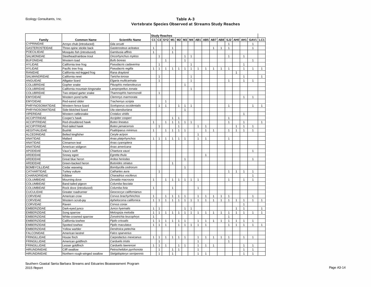
Ecology Consultants, Inc. Table A-3Vertebrate Species Observed at Streams Study Reaches
Southern Coastal Santa Barbara Streams and Estuaries Bioassessment Program2015 Report Page A3-14
C1 C3 SY2 M1 M2 M3 M4 AB1 AB5 AB7 AB8 SJ2 AH0 AH1 GAV1 LC1CYPRINIDAE Arroyo chub (introduced) Gila orcutti 1 1GASTEROSTEIDAE Three-spine stickle back Gasterosteus acleatus 1 1 1 1 1 1POECILIIDAE Mosquito fish (introduced) Gambusia affinis 1 1SALMONIDAE Steelhead/rainbow trout Oncorhynchus mykiss 1 1 1 1 1BUFONIDAE Western toad Bufo boreas 1 1 1HYLIDAE California tree frog Pseudacris cadaverina 1 1 1HYLIDAE Pacific tree frog Pseudacris regilla 1 1 1 1 1 1 1 1 1 1 1 1 1 1 1RANIDAE California red-legged frog Rana draytonii 1SALMANDRIDAE California newt Taricha torosa 1 1 1 1ANGUIDAE Alligator lizard Elgaria multicarinata 1 1 1 1 1COLUBRIDAE Gopher snake Pituophis melanoleucus 1COLUBRIDAE California mountain kingsnake Lampropeltus zonata 1COLUBRIDAE Two-striped garter snake ThamnophIs hammondii 1EMYDIDAE Western pond turtle Clemmys marmorata 1 1EMYDIDAE Red-eared slider Trachemys scripta 1PHRYNOSOMATIDAE Western fence lizard Sceloporus occidentalis 1 1 1 1 1 1 1 1PHRYNOSOMATIDAE Side-blotched lizard Uta stansburiana 1VIPERIDAE Western rattlesnake Crotalus viridis 1ACCIPITRIDAE Cooper's hawk Accipiter cooperi 1 1 1ACCIPITRIDAE Red-shouldered hawk Buteo lineatus 1 1 1 1 1 1 1 1 1ACCIPITRIDAE Red-tailed hawk Buteo jamaicensis 1 1 1 1 1 1 1AEGITHALIDAE Bushtit Psaltriparus minimus 1 1 1 1 1 1 1 1 1 1 1ALCEDINIDAE Belted kingfisher Ceryle aclyon 1ANATIDAE Mallard Anas platyrhynchos 1 1 1 1 1 1 1 1 1ANATIDAE Cinnamon teal Anas cyanopteraANATIDAE American widgeon Anas americanaAPODIDAE Vaux's swift Chaetura vauxi 1ARDEIDAE Snowy egret Egretta thula 1ARDEIDAE Great blue heron Ardea heriodas 1 1ARDEIDAE Green-backed heron Butorides striatus 1BOMBYCILLIDAE Cedar waxwing Bombycilla cedrorum 1CATHARTIDAE Turkey vulture Cathartes aura 1 1 1 1 1CHARADRIIDAE Killdeer Charadrius vociferus 1COLUMBIDAE Mourning dove Zenaida macroura 1 1 1 1 1 1 1 1 1 1COLUMBIDAE Band-tailed pigeon Columba fasciataCOLUMBIDAE Rock dove (introduced) Columba livia 1 1 1CUCULIDAE Greater roadrunner Geococcyx californianusCORVIDAE American crow Corvus brachyrhinchos 1 1 1 1 1 1 1 1 1 1 1CORVIDAE Western scrub-jay Aphelocoma californica 1 1 1 1 1 1 1 1 1 1 1 1 1 1 1 1CORVIDAE Raven Corvus corax 1EMBERIZIDAE Dark-eyed junco Junco hyemalis 1 1 1 1 1 1 1EMBERIZIDAE Song sparrow Melospiza melodia 1 1 1 1 1 1 1 1 1 1 1 1 1 1 1 1EMBERIZIDAE White-crowned sparrow Zonotrichia leucophrys 1 1EMBERIZIDAE California towhee Pipilo crissalis 1 1 1 1 1 1 1 1 1 1 1 1 1 1EMBERIZIDAE Spotted towhee Pipilo maculatus 1 1 1 1 1 1 1 1 1 1 1 1 1EMBERIZIDAE Yellow warbler Dendroica petechiaFALCONIDAE American kestrel Falco sparveriusFRINGILLIDAE House finch Carpodactus mexicanus 1 1 1 1 1 1 1 1 1 1 1 1 1FRINGILLIDAE American goldfinch Carduelis tristis 1 1 1FRINGILLIDAE Lesser goldfinch Carduelis lawrencei 1 1 1 1 1 1 1 1 1 1HIRUNDINIDAE Cilff swallow Petrochelidon pyrrhonota 1 1 1 1 1 1HIRUNDINIDAE Northern rough-winged swallow Stelgidopteryx serripennis 1 1 1 1 1 1
Family Common Name Scientific NameStudy Reaches

Ecology Consultants, Inc. Table A-3Vertebrate Species Observed at Streams Study Reaches
Southern Coastal Santa Barbara Streams and Estuaries Bioassessment Program2015 Report Page A3-15
C1 C3 SY2 M1 M2 M3 M4 AB1 AB5 AB7 AB8 SJ2 AH0 AH1 GAV1 LC1Family Common Name Scientific NameStudy Reaches
HIRUNDINIDAE Tree swallow Tachycineta bicolor 1HIRUNDINIDAE Violet-green swallow Trachycineta bicolor 1 1ICTERIDAE Blackbird, red-winged Agelaius phoeniceus 1ICTERIDAE Bullock's northern oriole Icterus galbula bullockii 1ICTERIDAE Hooded oriole Icterus cucullatus 1 1LARIDAE Western gull Larus occidentalis 1 1 1 1MIMIDAE Northern mockingbird Mimus polyglottos 1 1 1 1 1 1MIMIDAE California thrasher Toxostoma redivivum 1ODONTOPHORIDAE California quail Callipepla californica 1PARIDAE Plain oak titmouse Baeolopus inornatus 1 1 1 1 1PARULIDAE Common yellowthroat Geothlypis trichas 1 1 1 1 1 1 1 1 1 1 1PASSERIAE House sparrow (introduced) Passer domesticus 1 1 1PICIDAE Northern flicker Colaptes aurutus 1 1 1 1 1PICIDAE Acorn woodpecker Melanerpes formicivorus 1 1 1 1 1 1 1 1PICIDAE Downy woodpecker Picoides pubescens 1PICIDAE Hairy woodpecker Picoides villosus 1PODICIPEDIDAE Clark's grebe Aechmophorus clarkii 1PTILOGONATIDAE Phainopepla Phainopepla nitens 1 1RALLIDAE American coot Fulica americana 1REGULIDAE Ruby-crowned kinglet Regulus calendulaSTURNIDAE European starling (introduced) Sturnus vulgaris 1THRAUPIDAE Western tanager Piranga ludoviciana 1 1TIMALIIDAE Wrentit Chamaea fasciata 1 1 1 1 1 1 1 1 1 1TROCHILIDAE Anna's hummingbird Calypte anna 1 1 1 1 1 1 1 1 1 1 1TROCHILIDAE Rufous hummingbird Selasphorus rufus 1 1 1TROGLODYTIDAE Bewick's wren Thryomanes bewickii 1 1 1 1TROGLODYTIDAE Canyon wren Catherpes mexicanus 1 1TURDIDAE American robin Turdus migratorius 1TURDIDAE Hermit thrush Catharus guttatusTURDIDAE Swainson's thrush Catharus ustulatusTYRANNIDAE Pacific-slope flycatcher Empidonax difficilis 1 1 1 1 1 1 1 1 1TYRANNIDAE Black phoebe Sayornis nigricans 1 1 1 1 1 1 1 1 1 1 1 1 1 1 1 1TYRANNIDAE Western kingbird Tyrannus verticalis 1TYRANNIDAE Western wood-pewee Contopus sordidulus 1CANIDAE Coyote Canis latrans 1 1 1 1CERVIDAE Mule deer Odocoileus hemionus 1 1 1 1 1DIDELPHIDAE Oppossum (introduced) Didelphis virginiana 1FELIDAE Bobcat Lynx rufus 1 1 1LEPORIDAE Cottontail rabbit Sylvilagus auduboniLEPORIDAE Brush rabbit Sylvilagus bachmanni 1MEPHITIDAE Striped skunk M. mephitis 1PROCYONIDAE Racoon Procyon lotor 1 1 1 1 1 1 1 1 1 1 1SCIRIDAE Merriam's chipmunk Eutamias merriamiSCIRIDAE California ground squirrel Spermophilus beecheyi 1 1SCIRIDAE Western gray squirrel Sciurus griseusTALPIDAE Broad-footed mole Scapanus latimanus 1URSIDAE Black bear Ursus americanus 1
30 37 26 25 24 29 21 30 22 10 8 32 14 36 36 132 5 2 2 1 3 4 1 1 2 2 3 1 5 4 2
# vertebrate species# native aquatic vertebrate species
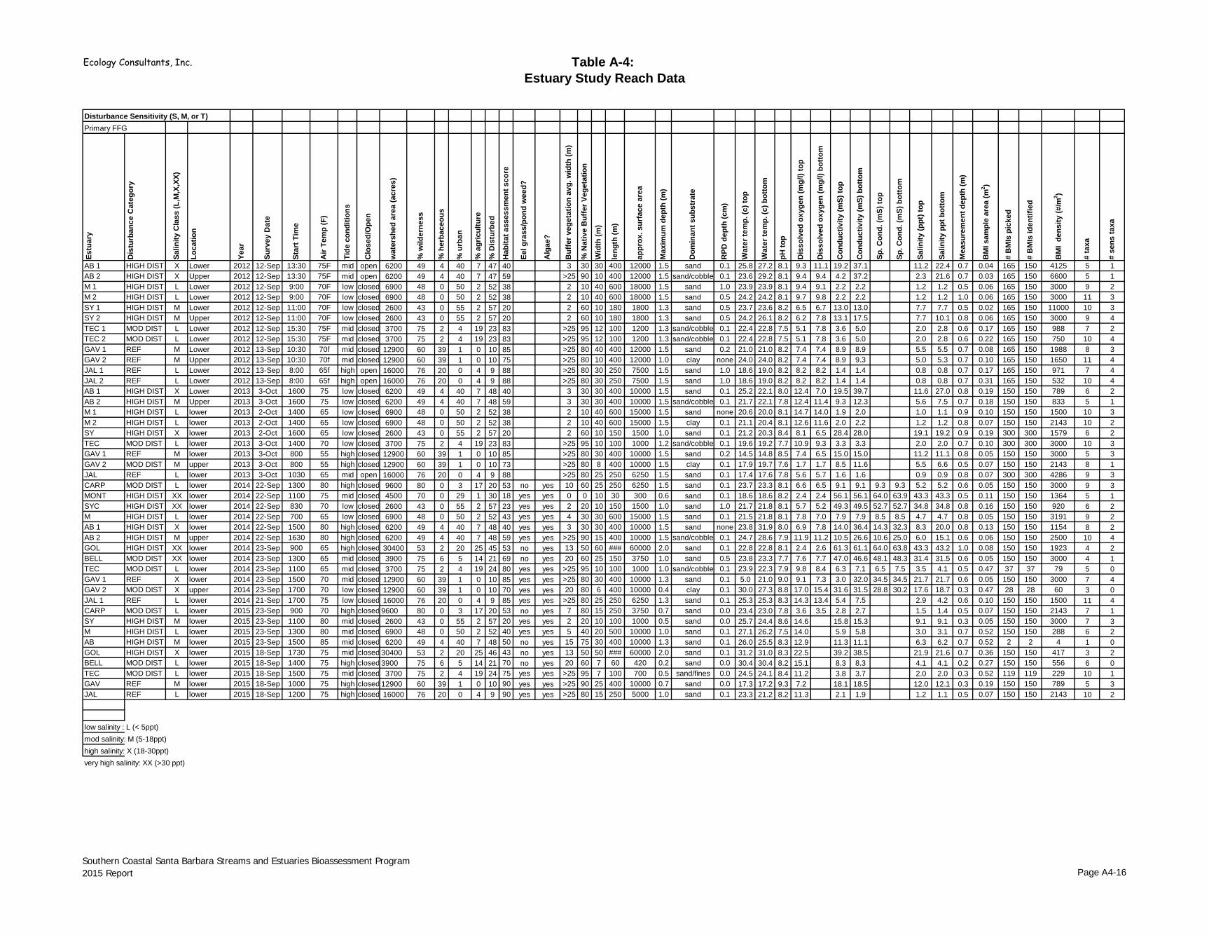
Ecology Consultants, Inc. Table A-4: Estuary Study Reach Data
Southern Coastal Santa Barbara Streams and Estuaries Bioassessment Program2015 Report Page A4-16
Disturbance Sensitivity (S, M, or T) Primary FFG
Estu
ary
Dis
turb
ance
Cat
egor
y
Salin
ity C
lass
(L,M
,X,X
X)
Loca
tion
Year
Surv
ey D
ate
Star
t Tim
e
Air
Tem
p (F
)
Tide
con
ditio
ns
Clo
sed/
Ope
n
wat
ersh
ed a
rea
(acr
es)
% w
ilder
ness
% h
erba
ceou
s
% u
rban
% a
gric
ultu
re
% D
istu
rbed
Hab
itat a
sses
smen
t sco
re
Eel g
rass
/pon
d w
eed?
Alg
ae?
Buf
fer v
eget
atio
n av
g. w
idth
(m)
% N
ativ
e B
uffe
r Veg
etat
ion
Wid
th (m
)
leng
th (m
)
appr
ox. s
urfa
ce a
rea
Max
imum
dep
th (m
)
Dom
inan
t sub
stra
te
RPD
dep
th (c
m)
Wat
er te
mp.
(c) t
op
Wat
er te
mp.
(c) b
otto
m
pH to
p
Dis
solv
ed o
xyge
n (m
g/l)
top
Dis
solv
ed o
xyge
n (m
g/l)
botto
m
Con
duct
ivity
(mS)
top
Con
duct
ivity
(mS)
bot
tom
Sp. C
ond.
(mS)
top
Sp. C
ond.
(mS)
bot
tom
Salin
ity (p
pt) t
op
Salin
ity p
pt b
otto
m
Mea
sure
men
t dep
th (m
)
BM
I sam
ple
area
(m2 )
# B
MIs
pic
ked
# B
MIs
iden
tifie
d
BM
I de
nsity
(#/m
2 )
# ta
xa
# se
ns ta
xa
AB 1 HIGH DIST X Lower 2012 12-Sep 13:30 75F mid open 6200 49 4 40 7 47 40 3 30 30 400 12000 1.5 sand 0.1 25.8 27.2 8.1 9.3 11.1 19.2 37.1 11.2 22.4 0.7 0.04 165 150 4125 5 1AB 2 HIGH DIST X Upper 2012 12-Sep 13:30 75F mid open 6200 49 4 40 7 47 59 >25 90 10 400 12000 1.5 sand/cobble 0.1 23.6 29.2 8.1 9.4 9.4 4.2 37.2 2.3 21.6 0.7 0.03 165 150 6600 5 1M 1 HIGH DIST L Lower 2012 12-Sep 9:00 70F low closed 6900 48 0 50 2 52 38 2 10 40 600 18000 1.5 sand 1.0 23.9 23.9 8.1 9.4 9.1 2.2 2.2 1.2 1.2 0.5 0.06 165 150 3000 9 2M 2 HIGH DIST L Lower 2012 12-Sep 9:00 70F low closed 6900 48 0 50 2 52 38 2 10 40 600 18000 1.5 sand 0.5 24.2 24.2 8.1 9.7 9.8 2.2 2.2 1.2 1.2 1.0 0.06 165 150 3000 11 3SY 1 HIGH DIST M Lower 2012 12-Sep 11:00 70F low closed 2600 43 0 55 2 57 20 2 60 10 180 1800 1.3 sand 0.5 23.7 23.6 8.2 6.5 6.7 13.0 13.0 7.7 7.7 0.5 0.02 165 150 11000 10 3SY 2 HIGH DIST M Upper 2012 12-Sep 11:00 70F low closed 2600 43 0 55 2 57 20 2 60 10 180 1800 1.3 sand 0.5 24.2 26.1 8.2 6.2 7.8 13.1 17.5 7.7 10.1 0.8 0.06 165 150 3000 9 4TEC 1 MOD DIST L Lower 2012 12-Sep 15:30 75F mid closed 3700 75 2 4 19 23 83 >25 95 12 100 1200 1.3 sand/cobble 0.1 22.4 22.8 7.5 5.1 7.8 3.6 5.0 2.0 2.8 0.6 0.17 165 150 988 7 2TEC 2 MOD DIST L Lower 2012 12-Sep 15:30 75F mid closed 3700 75 2 4 19 23 83 >25 95 12 100 1200 1.3 sand/cobble 0.1 22.4 22.8 7.5 5.1 7.8 3.6 5.0 2.0 2.8 0.6 0.22 165 150 750 10 4GAV 1 REF M Lower 2012 13-Sep 10:30 70f mid closed 12900 60 39 1 0 10 85 >25 80 40 400 12000 1.5 sand 0.2 21.0 21.0 8.2 7.4 7.4 8.9 8.9 5.5 5.5 0.7 0.08 165 150 1988 8 3GAV 2 REF M Upper 2012 13-Sep 10:30 70f mid closed 12900 60 39 1 0 10 75 >25 80 10 400 12000 1.0 clay none 24.0 24.0 8.2 7.4 7.4 8.9 9.3 5.0 5.3 0.7 0.10 165 150 1650 11 4JAL 1 REF L Lower 2012 13-Sep 8:00 65f high open 16000 76 20 0 4 9 88 >25 80 30 250 7500 1.5 sand 1.0 18.6 19.0 8.2 8.2 8.2 1.4 1.4 0.8 0.8 0.7 0.17 165 150 971 7 4JAL 2 REF L Lower 2012 13-Sep 8:00 65f high open 16000 76 20 0 4 9 88 >25 80 30 250 7500 1.5 sand 1.0 18.6 19.0 8.2 8.2 8.2 1.4 1.4 0.8 0.8 0.7 0.31 165 150 532 10 4AB 1 HIGH DIST X Lower 2013 3-Oct 1600 75 low closed 6200 49 4 40 7 48 40 3 30 30 400 10000 1.5 sand 0.1 25.2 22.1 8.0 12.4 7.0 19.5 39.7 11.6 27.0 0.8 0.19 150 150 789 6 2AB 2 HIGH DIST M Upper 2013 3-Oct 1600 75 low closed 6200 49 4 40 7 48 59 3 30 30 400 10000 1.5 sand/cobble 0.1 21.7 22.1 7.8 12.4 11.4 9.3 12.3 5.6 7.5 0.7 0.18 150 150 833 5 1M 1 HIGH DIST L lower 2013 2-Oct 1400 65 low closed 6900 48 0 50 2 52 38 2 10 40 600 15000 1.5 sand none 20.6 20.0 8.1 14.7 14.0 1.9 2.0 1.0 1.1 0.9 0.10 150 150 1500 10 3M 2 HIGH DIST L lower 2013 2-Oct 1400 65 low closed 6900 48 0 50 2 52 38 2 10 40 600 15000 1.5 clay 0.1 21.1 20.4 8.1 12.6 11.6 2.0 2.2 1.2 1.2 0.8 0.07 150 150 2143 10 2SY HIGH DIST X lower 2013 2-Oct 1600 65 low closed 2600 43 0 55 2 57 20 2 60 10 150 1500 1.0 sand 0.1 21.2 20.3 8.4 8.1 6.5 28.4 28.0 19.1 19.2 0.9 0.19 300 300 1579 6 2TEC MOD DIST L lower 2013 3-Oct 1400 70 low closed 3700 75 2 4 19 23 83 >25 95 10 100 1000 1.2 sand/cobble 0.1 19.6 19.2 7.7 10.9 9.3 3.3 3.3 2.0 2.0 0.7 0.10 300 300 3000 10 3GAV 1 REF M lower 2013 3-Oct 800 55 high closed 12900 60 39 1 0 10 85 >25 80 30 400 10000 1.5 sand 0.2 14.5 14.8 8.5 7.4 6.5 15.0 15.0 11.2 11.1 0.8 0.05 150 150 3000 5 3GAV 2 MOD DIST M upper 2013 3-Oct 800 55 high closed 12900 60 39 1 0 10 73 >25 80 8 400 10000 1.5 clay 0.1 17.9 19.7 7.6 1.7 1.7 8.5 11.6 5.5 6.6 0.5 0.07 150 150 2143 8 1JAL REF L lower 2013 3-Oct 1030 65 mid open 16000 76 20 0 4 9 88 >25 80 25 250 6250 1.5 sand 0.1 17.4 17.6 7.8 5.6 5.7 1.6 1.6 0.9 0.9 0.8 0.07 300 300 4286 9 3CARP MOD DIST L lower 2014 22-Sep 1300 80 high closed 9600 80 0 3 17 20 53 no yes 10 60 25 250 6250 1.5 sand 0.1 23.7 23.3 8.1 6.6 6.5 9.1 9.1 9.3 9.3 5.2 5.2 0.6 0.05 150 150 3000 9 3MONT HIGH DIST XX lower 2014 22-Sep 1100 75 mid closed 4500 70 0 29 1 30 18 yes yes 0 0 10 30 300 0.6 sand 0.1 18.6 18.6 8.2 2.4 2.4 56.1 56.1 64.0 63.9 43.3 43.3 0.5 0.11 150 150 1364 5 1SYC HIGH DIST XX lower 2014 22-Sep 830 70 low closed 2600 43 0 55 2 57 23 yes yes 2 20 10 150 1500 1.0 sand 1.0 21.7 21.8 8.1 5.7 5.2 49.3 49.5 52.7 52.7 34.8 34.8 0.8 0.16 150 150 920 6 2M HIGH DIST L lower 2014 22-Sep 700 65 low closed 6900 48 0 50 2 52 43 yes yes 4 30 30 600 15000 1.5 sand 0.1 21.5 21.8 8.1 7.8 7.0 7.9 7.9 8.5 8.5 4.7 4.7 0.8 0.05 150 150 3191 9 2AB 1 HIGH DIST X lower 2014 22-Sep 1500 80 high closed 6200 49 4 40 7 48 40 yes yes 3 30 30 400 10000 1.5 sand none 23.8 31.9 8.0 6.9 7.8 14.0 36.4 14.3 32.3 8.3 20.0 0.8 0.13 150 150 1154 8 2AB 2 HIGH DIST M upper 2014 22-Sep 1630 80 high closed 6200 49 4 40 7 48 59 yes yes >25 90 15 400 10000 1.5 sand/cobble 0.1 24.7 28.6 7.9 11.9 11.2 10.5 26.6 10.6 25.0 6.0 15.1 0.6 0.06 150 150 2500 10 4GOL HIGH DIST XX lower 2014 23-Sep 900 65 high closed 30400 53 2 20 25 45 53 no yes 13 50 60 ### 60000 2.0 sand 0.1 22.8 22.8 8.1 2.4 2.6 61.3 61.1 64.0 63.8 43.3 43.2 1.0 0.08 150 150 1923 4 2BELL MOD DIST XX lower 2014 23-Sep 1300 65 mid closed 3900 75 6 5 14 21 69 no yes 20 60 25 150 3750 1.0 sand 0.5 23.8 23.3 7.7 7.6 7.7 47.0 46.6 48.1 48.3 31.4 31.5 0.6 0.05 150 150 3000 4 1TEC MOD DIST L lower 2014 23-Sep 1100 65 mid closed 3700 75 2 4 19 24 80 yes yes >25 95 10 100 1000 1.0 sand/cobble 0.1 23.9 22.3 7.9 9.8 8.4 6.3 7.1 6.5 7.5 3.5 4.1 0.5 0.47 37 37 79 5 0GAV 1 REF X lower 2014 23-Sep 1500 70 mid closed 12900 60 39 1 0 10 85 yes yes >25 80 30 400 10000 1.3 sand 0.1 5.0 21.0 9.0 9.1 7.3 3.0 32.0 34.5 34.5 21.7 21.7 0.6 0.05 150 150 3000 7 4GAV 2 MOD DIST X upper 2014 23-Sep 1700 70 low closed 12900 60 39 1 0 10 70 yes yes 20 80 6 400 10000 0.4 clay 0.1 30.0 27.3 8.8 17.0 15.4 31.6 31.5 28.8 30.2 17.6 18.7 0.3 0.47 28 28 60 3 0JAL 1 REF L lower 2014 21-Sep 1700 75 low closed 16000 76 20 0 4 9 85 yes yes >25 80 25 250 6250 1.3 sand 0.1 25.3 25.3 8.3 14.3 13.4 5.4 7.5 2.9 4.2 0.6 0.10 150 150 1500 11 4CARP MOD DIST L lower 2015 23-Sep 900 70 high closed 9600 80 0 3 17 20 53 no yes 7 80 15 250 3750 0.7 sand 0.0 23.4 23.0 7.8 3.6 3.5 2.8 2.7 1.5 1.4 0.5 0.07 150 150 2143 7 1SY HIGH DIST M lower 2015 23-Sep 1100 80 mid closed 2600 43 0 55 2 57 20 yes yes 2 20 10 100 1000 0.5 sand 0.0 25.7 24.4 8.6 14.6 15.8 15.3 9.1 9.1 0.3 0.05 150 150 3000 7 3M HIGH DIST L lower 2015 23-Sep 1300 80 mid closed 6900 48 0 50 2 52 40 yes yes 5 40 20 500 10000 1.0 sand 0.1 27.1 26.2 7.5 14.0 5.9 5.8 3.0 3.1 0.7 0.52 150 150 288 6 2AB HIGH DIST M lower 2015 23-Sep 1500 85 mid closed 6200 49 4 40 7 48 50 no yes 15 75 30 400 10000 1.3 sand 0.1 26.0 25.5 8.3 12.9 11.3 11.1 6.3 6.2 0.7 0.52 2 2 4 1 0GOL HIGH DIST X lower 2015 18-Sep 1730 75 mid closed 30400 53 2 20 25 46 43 no yes 13 50 50 ### 60000 2.0 sand 0.1 31.2 31.0 8.3 22.5 39.2 38.5 21.9 21.6 0.7 0.36 150 150 417 3 2BELL MOD DIST L lower 2015 18-Sep 1400 75 high closed 3900 75 6 5 14 21 70 no yes 20 60 7 60 420 0.2 sand 0.0 30.4 30.4 8.2 15.1 8.3 8.3 4.1 4.1 0.2 0.27 150 150 556 6 0TEC MOD DIST L lower 2015 18-Sep 1500 75 mid closed 3700 75 2 4 19 24 75 yes yes >25 95 7 100 700 0.5 sand/fines 0.0 24.5 24.1 8.4 11.2 3.8 3.7 2.0 2.0 0.3 0.52 119 119 229 10 1GAV REF M lower 2015 18-Sep 1000 75 high closed 12900 60 39 1 0 10 90 yes yes >25 90 25 400 10000 0.7 sand 0.0 17.3 17.2 9.3 7.2 18.1 18.5 12.0 12.1 0.3 0.19 150 150 789 5 3JAL REF L lower 2015 18-Sep 1200 75 high closed 16000 76 20 0 4 9 90 yes yes >25 80 15 250 5000 1.0 sand 0.1 23.3 21.2 8.2 11.3 2.1 1.9 1.2 1.1 0.5 0.07 150 150 2143 10 2
low salinity : L (< 5ppt)mod salinity: M (5-18ppt)high salinity: X (18-30ppt)very high salinity: XX (>30 ppt)

Ecology Consultants, Inc. Table A-4: Estuary Study Reach Data
Southern Coastal Santa Barbara Streams and Estuaries Bioassessment Program2015 Report Page A4-17
Disturbance Primary FFG
Estu
ary
AB 1AB 2M 1M 2SY 1SY 2TEC 1TEC 2GAV 1GAV 2JAL 1JAL 2AB 1AB 2M 1M 2SYTECGAV 1GAV 2JALCARPMONTSYCM AB 1AB 2GOLBELLTECGAV 1GAV 2JAL 1CARPSYMABGOLBELLTECGAVJAL
low salinity : mod salinity: high salinity: very high sal
S NA T NA NA NA M NA NA NA T NA NA T NA NA NA S M NA M NA S M T M T NA S ??? S S T M NA T NAcg sh p p p p cg cg p p NA p cg p NA p p p p p p cg p sc cg cg cg sh cg cg cg cg cg cg cf cf pa
# to
l tax
a
#sen
s/#t
ol
% in
sect
s
%no
n-in
sect
s
% d
omin
ant t
axa
% 2
dom
inan
t tax
a
% p
reda
tors
%co
llect
or-g
athe
rers
100+
(%cg
- %
pred
)
% S
ensi
tive
BM
Is
% T
oler
ant B
MIs
Bae
tidae
Dry
opid
ae
Dyt
isci
dae
Hal
ipid
ae
Hyd
roph
ilida
e
Cer
atop
ogon
idae
Chi
rono
mid
ae
Cul
icid
ae
Dol
icho
podi
dae
Empi
dida
e
Ephy
drid
ae
Mus
cida
e
Stra
tiom
yida
e
Cor
ixid
ae
Velii
dae
Not
onec
tidae
Ger
ridae
Aes
hnid
ae
Coe
nagr
ioni
dae
Lest
idae
Libe
lulii
dae
CO
LLEM
BO
LA
AC
AR
I
GA
STR
OPO
DA
OST
RA
CO
DA
CO
PEPO
DA
CLA
DO
CER
A
DEC
APO
DA
-Hip
pida
e-Em
erita
ana
lo
AM
PHIP
OD
A (G
amm
arid
ae)
AM
PHIP
OD
A (C
orop
hiid
ae)
Mys
tidac
ea (S
hrim
p)
ISO
POD
A
OLI
GO
CH
AET
A
POLY
CH
AET
A
Biv
alvi
a-cl
am
Biv
alvi
a (m
usse
l)
HIR
UD
INEA
2 0.5 37 63 61 97 35 65 129 1 97 0 0 0 0 0 0 2 0 0 0 0 0 0 53 0 0 0 0 0 0 0 0 0 0 92 1 0 0 2 0 0 0 0 0 0 0 03 0.3 68 32 65 85 65 35 71 1 95 0 0 0 0 0 0 5 0 0 0 0 0 0 97 0 0 0 0 0 0 0 0 0 0 31 0 0 0 2 0 0 0 15 0 0 0 04 0.5 19 80 46 74 2 93 191 3 75 3 0 1 0 0 0 23 0 1 0 0 0 0 1 0 0 0 0 0 0 0 0 0 7 42 0 69 0 0 0 0 2 0 0 0 0 04 0.8 26 74 53 70 5 93 188 11 72 15 0 2 0 0 0 18 0 0 0 0 0 0 1 0 0 0 0 1 0 2 0 1 4 25 0 80 0 0 0 0 1 0 0 0 0 05 0.6 79 21 43 72 46 54 108 7 64 7 0 3 0 0 0 43 0 0 0 0 0 0 65 0 0 0 0 0 0 1 0 0 0 25 0 1 0 2 0 0 1 2 0 0 0 04 1.0 50 50 35 62 17 83 165 11 53 8 0 2 0 0 0 41 0 0 0 0 0 0 24 0 0 0 0 0 0 0 0 0 0 52 0 0 0 1 0 0 8 2 12 0 0 04 0.5 75 25 41 68 27 72 145 7 52 9 0 0 0 0 0 61 0 0 0 1 0 0 41 0 0 0 0 0 0 0 0 0 0 1 0 35 0 0 0 0 2 0 0 0 0 03 1.3 71 29 43 67 23 76 153 8 47 5 0 0 0 0 0 65 0 0 0 1 0 1 34 0 0 0 0 0 0 0 0 1 0 0 1 36 0 1 0 0 5 0 0 0 0 03 1.0 13 87 43 73 5 95 191 55 35 0 0 0 0 0 0 12 0 1 0 0 0 0 6 0 0 0 0 0 0 0 0 0 0 46 0 1 0 65 0 0 17 0 2 0 0 03 1.3 77 23 66 80 7 92 185 91 5 99 1 2 0 0 0 4 1 0 0 0 0 0 3 0 0 0 5 1 0 0 0 0 0 2 0 0 0 21 0 0 11 0 0 0 0 01 4.0 20 80 56 72 2 98 196 68 16 6 0 0 0 0 0 23 0 0 0 0 1 0 0 0 0 0 0 0 0 0 0 2 0 24 0 0 0 0 0 10 84 0 0 0 0 03 1.3 25 75 40 58 3 97 194 59 21 10 0 0 0 0 0 24 0 0 0 0 0 0 4 0 0 0 0 0 0 0 0 0 1 27 5 1 0 15 0 3 60 0 0 0 0 04 0.5 12 86 69 81 11 86 175 5 88 0 0 0 0 0 0 0 0 0 0 1 0 0 17 0 0 0 0 0 0 0 0 0 0 104 0 0 0 7 0 0 0 10 8 0 0 03 0.3 93 7 91 95 91 9 17 2 96 0 0 0 0 0 0 3 0 0 0 0 0 0 137 0 0 0 0 0 0 0 0 0 0 6 0 0 0 3 0 0 0 1 0 0 0 04 0.8 36 64 33 51 20 70 150 25 55 10 0 2 0 0 0 14 0 0 0 0 0 0 28 0 0 0 0 0 0 0 0 0 15 49 1 3 0 2 0 0 26 0 0 0 0 03 0.7 12 88 60 83 1 77 176 7 63 7 0 0 0 0 0 10 0 0 0 0 0 0 1 0 0 0 0 0 0 0 0 0 34 90 0 4 0 0 0 0 4 0 0 0 0 03 0.7 56 44 56 95 56 44 88 1 95 0 0 0 0 0 0 0 0 0 0 0 0 0 168 0 0 0 0 0 0 0 0 0 0 117 8 0 0 0 0 0 3 1 3 0 0 03 1.0 69 31 46 66 7 93 187 24 28 50 0 0 0 0 0 138 0 0 0 0 0 0 18 0 0 0 0 1 0 1 0 0 0 60 3 0 0 10 0 0 13 6 0 0 0 01 3.0 23 77 53 76 0 100 200 63 3 0 0 0 0 0 0 34 0 0 0 0 0 0 0 0 0 0 0 0 0 0 0 0 0 4 0 0 0 80 0 0 14 0 18 0 0 02 0.5 99 1 39 76 40 60 120 39 38 59 0 0 0 0 0 29 0 0 0 0 0 0 55 1 2 0 0 1 0 2 0 0 0 0 0 0 0 0 0 0 0 2 0 0 0 03 1.0 69 31 43 61 19 67 148 44 31 129 0 0 0 0 0 26 0 0 0 0 0 0 53 0 0 0 0 0 0 0 0 3 44 24 4 16 0 0 0 0 1 0 0 0 0 03 1.0 52 48 38 68 7 93 187 31 48 44 0 3 0 0 0 25 0 0 0 0 0 0 0 0 0 0 0 4 0 2 0 1 0 12 0 0 0 0 0 0 2 57 0 0 0 03 0.3 23 87 77 97 1 89 187 0 97 0 0 0 0 0 1 3 0 0 0 29 0 0 1 0 0 0 0 0 0 0 0 0 0 0 0 0 0 0 0 0 0 116 14 0 0 01 2.0 17 73 71 88 17 73 155 2 17 0 0 0 0 0 0 0 0 0 0 0 0 0 26 0 0 0 0 0 0 0 0 0 0 0 0 0 0 0 106 0 3 0 0 1 0 04 0.5 36 64 41 62 10 80 170 5 63 7 0 11 0 0 0 32 0 0 0 0 0 0 3 0 0 0 0 0 0 1 0 0 15 61 0 0 0 0 0 0 1 19 0 0 0 04 0.5 95 5 78 92 79 21 41 1 83 1 0 2 0 0 0 21 2 0 0 0 0 0 117 0 0 0 0 0 0 0 0 0 0 4 0 0 0 1 0 0 0 2 0 0 0 03 1.3 57 43 41 67 41 59 117 9 80 8 0 0 0 0 0 14 1 0 0 0 0 0 61 0 0 0 1 0 0 0 0 0 0 40 1 0 0 4 0 0 1 19 0 0 0 02 1.0 18 82 56 74 18 82 164 0 30 0 0 0 0 0 0 0 0 0 0 0 0 0 27 0 0 0 0 0 0 0 0 0 0 18 0 0 0 0 84 0 0 0 21 0 0 02 0.5 99 1 80 95 95 1 7 0 84 0 0 0 0 0 22 0 0 0 0 6 0 0 120 0 0 0 0 0 0 0 0 0 0 0 0 0 0 0 0 0 0 0 2 0 0 02 0.0 30 70 32 59 3 84 181 0 57 0 0 0 0 1 0 10 0 0 0 0 0 0 0 0 0 0 0 0 0 0 0 0 5 9 0 0 0 0 0 0 0 12 0 0 0 02 2.0 4 96 41 69 1 99 199 42 42 0 0 0 0 0 0 5 0 0 0 0 0 0 1 0 0 0 0 0 0 0 0 0 0 62 0 0 0 15 0 6 42 0 19 0 0 02 0.0 93 7 64 93 29 71 143 0 36 0 0 0 0 0 0 18 0 0 0 0 0 0 8 0 0 0 0 0 0 0 0 0 0 2 0 0 0 0 0 0 0 0 0 0 0 05 0.8 50 56 43 71 11 87 177 25 53 33 0 1 0 0 0 29 0 0 0 0 0 0 11 0 0 0 1 0 0 0 0 3 12 64 0 3 0 0 0 1 0 1 0 0 0 04 0.3 57 43 49 69 2 90 188 5 37 8 0 3 0 0 0 74 0 0 0 0 0 0 0 0 0 0 0 0 0 0 0 0 12 2 0 21 0 0 0 0 0 30 0 0 0 03 1.0 58 35 43 72 44 49 105 1 75 1 0 0 0 0 0 20 0 0 0 0 0 0 65 0 1 0 0 0 0 0 0 0 0 43 0 0 0 1 0 0 0 5 4 0 0 03 0.7 19 81 48 67 0 81 181 15 71 7 0 0 0 0 0 22 0 0 0 0 0 0 0 0 0 0 0 0 0 0 0 0 0 72 0 0 0 15 0 0 0 5 0 0 29 00 0.0 100 0 100 100 0 100 200 0 0 0 0 0 0 0 0 2 0 0 0 0 0 0 0 0 0 0 0 0 0 0 0 0 0 0 0 0 0 0 0 0 0 0 0 0 0 01 2.0 0 100 40 71 0 59 159 0 32 0 0 0 0 0 0 0 0 0 0 0 0 0 0 0 0 0 0 0 0 0 0 0 0 48 0 0 0 0 62 0 0 0 40 0 0 04 0.0 23 77 77 83 19 77 158 0 90 0 0 4 0 0 14 0 0 1 0 7 0 0 9 0 0 0 0 0 0 0 0 0 0 115 0 0 0 0 0 0 0 0 0 0 0 02 0.5 51 49 37 62 24 69 145 6 38 0 0 0 0 11 0 30 0 10 0 1 0 0 0 1 0 0 0 8 0 0 0 0 6 44 1 0 0 7 0 0 0 0 0 0 0 02 1.5 1 99 43 80 1 99 199 59 40 0 0 0 0 0 0 0 0 0 0 0 0 0 1 0 0 0 0 0 0 0 0 0 0 59 0 0 0 21 0 0 68 0 1 0 0 04 0.5 82 18 40 70 33 54 121 43 35 62 0 0 0 0 0 11 0 0 0 0 0 0 46 0 2 0 0 0 0 2 0 0 19 2 0 3 0 2 0 0 0 1 0 0 0 0

Ecology Consultants, Inc. Table A-5ANOVAs of BMI Metrics by Disturbance Group and Flow Group
Southern Coastal Santa Barbara Streams and Estuaries Bioassessment Program2015 Report Page A5-18
Disurbance GroupParameter r-square p Flow Group n Mean Std Error Lower 95% Upper 95%HIGH DIST IBI Score 0.08 0.39 F-F 22 13.0455 2.0084 8.9 17.191
F-P 4 14.25 4.71 4.53 23.971P-P 1 0 9.4201 -19.44 19.442
MOD DIST IBI Score 0.74 <0.0001 F-F 11 43.9091 2.7433 38.06 49.756F-P 6 18.1667 3.7144 10.25 26.084P-P 1 3 9.0985 -16.39 22.393
REF IBI Score 0.77 0.0006 F-F 9 51.1111 3.338 43.67 58.549F-P 3 22 5.782 9.12 34.883P-P 1 4 10.014 -18.31 26.314
REF+MOD DIST IBI Score 0.74 <0.0001 F-F 20 47.15 2.1261 42.79 51.505F-P 9 19.4444 3.1693 12.95 25.937P-P 2 3.5 6.7232 -10.27 17.272
# EPT families 0.54 <0.0001 F-F 20 10.75 0.6663 9.385 12.115F-P 9 5.1111 0.9933 3.076 7.146P-P 2 2 2.1071 -2.316 6.316
# Insect families 0.5 <0.0001 F-F 20 21.3 0.9889 19.274 23.326F-P 9 15.1111 1.4741 12.092 18.131P-P 2 6.5 3.127 0.095 12.905
% Plecoptera-Trichoptera0.45 0.0002 F-F 20 15.27 1.6729 11.84 18.697F-P 9 2.0939 2.4939 -3.01 7.202P-P 2 0 5.2903 -10.84 10.837
% shredders+predators 0.42 0.0005 F-F 20 15.9704 1.3008 13.31 18.635F-P 9 7.786 1.9392 3.81 11.758P-P 2 1.431 4.1136 -7 9.857
Tolerance value avg. 0.6 <0.0001 F-F 20 5.05608 0.17264 4.7024 5.4097F-P 9 6.74797 0.25735 6.2208 7.2751P-P 2 7.51905 0.54593 6.4008 8.6373
% sensitive BMIs 0.51 <0.0001 F-F 20 36.2123 3.113 29.84 42.589F-P 9 10.0712 4.6405 0.57 19.577P-P 2 0.9762 9.8441 -19.19 21.141
% tolerant BMIs 0.64 <0.0001 F-F 20 42.1705 3.289 35.432 48.91F-P 9 77.0749 4.904 67.03 87.12P-P 2 94.2619 10.402 72.954 115.57
BMI density 0.08 0.32 F-F 20 585.125 66.53 448.8 721.4F-P 9 412.307 99.18 209.2 615.46P-P 2 417.857 210.38 -13.1 848.81
Baetidae 0.12 0.18 F-F 20 26.1 5.676 14.47 37.728F-P 9 7.6667 8.462 -9.67 25P-P 2 8.5 17.95 -28.27 45.27
Caenidae 0.23 0.03 F-F 20 19.65 3.453 12.58 26.722F-P 9 3.5556 5.147 -6.99 14.098P-P 2 0.5 10.918 -21.86 22.864
Glossostomatidae 0.23 0.03 F-F 20 2.05 0.4246 1.18 2.9197F-P 9 0 0.6329 -1.296 1.2965P-P 2 0 1.3426 -2.75 2.7503
Lepidostomatidae 0.17 0.08 F-F 20 12.45 2.9574 6.39 18.508F-P 9 0.8889 4.4086 -8.14 9.92P-P 2 0 9.3521 -19.16 19.157
Rhyacophilidae 0.21 0.04 F-F 20 3 0.6175 1.735 4.265F-P 9 0.22222 0.9206 -1.663 2.1079P-P 2 0 1.9528 -4 4.0002
Dytisidae 0.43 0.0003 F-F 20 2.2 0.5874 0.997 3.4032F-P 9 6.66667 0.8756 4.873 8.4602P-P 2 0 1.8574 -3.805 3.8047

Ecology Consultants, Inc. Table A-5ANOVAs of BMI Metrics by Disturbance Group and Flow Group
Southern Coastal Santa Barbara Streams and Estuaries Bioassessment Program2015 Report Page A5-19
Elmidae 0.18 0.06 F-F 20 5.3 0.9696 3.314 7.286F-P 9 1.55556 1.4453 -1.405 4.5162P-P 2 0 3.066 -6.28 6.2804
Ceratopogonidae 0.27 0.01 F-F 20 3 0.4268 2.126 3.8742F-P 9 0.66667 0.6362 -0.637 1.9699P-P 2 1 1.3496 -1.765 3.7645
Chironomidae 0.19 0.05 F-F 20 79.55 11.422 56.153 102.95F-P 9 125 17.027 90.122 159.88P-P 2 143 36.119 69.013 216.99
Simulidae 0.23 0.03 F-F 20 8 5.585 -3.44 19.441F-P 9 35.6667 8.326 18.61 52.722P-P 2 0 17.663 -36.18 36.18
Non-insects 0.06 0.44 F-F 20 35.3 9.195 16.47 54.135F-P 9 56.5556 13.707 28.48 84.633P-P 2 38 29.076 -21.56 97.56

Ecology Consultants, Inc. Table A-6Results of One Way ANOVA of IBI Score by Year for REF Group
Southern Coastal Santa Barbara Streams and Estuaries Bioassessment Program2015 Report Page A6-20
REF Groupn=66p<0.0001r2=0.59
Year Number Mean Std Error Lower 95% Upper 95%2000 11 61 3.0 54.9 67.12001 4 57 5.0 46.6 66.92002 5 63 4.5 54.1 72.32003 5 60 4.5 51.3 69.52005 4 36 5.0 25.9 46.12006 4 59 5.0 48.6 68.92007 4 62 5.0 51.9 72.12008 4 54 5.0 44.1 64.42009 5 57 4.5 47.5 65.72010 3 61 5.8 49.6 73.02011 4 50 5.0 40.1 60.42012 3 57 5.8 45.6 69.02013 4 47 5.0 36.4 56.62014 3 33 5.8 21.3 44.72015 3 24 5.8 12.6 36.0

Ecology Consultants, Inc. Table A-7ANOVAs of IBI Score for HIGH DIST, MOD DIST, and REF Groups for Each Year (2000 to 2015)
Southern Coastal Santa Barbara Streams and Estuaries Bioassessment Program2015 Report Table A721
Year r-square p Group n Mean Std Error Lower 95% Upper 95%
2000 0.79 <0.0001 HIGH DIST 8 17.4 3.5 10.1 24.6
MOD DIST 8 48.9 3.5 41.6 56.1REF 11 61.0 3.0 54.8 67.2
2001 0.79 0.001 HIGH DIST 8 17.4 3.5 10.1 24.6
MOD DIST 8 48.9 3.5 41.6 56.1REF 11 61.0 3.0 54.8 67.2
2002 0.85 <0.0001 HIGH DIST 10 12.3 3.4 5.2 19.4
MOD DIST 5 56.0 4.8 45.9 66.1REF 5 63.2 4.8 53.1 73.3
2003 0.85 <0.0001 HIGH DIST 10 10.8 3.2 4.1 17.5
MOD DIST 5 42.4 4.5 32.9 51.9REF 5 60.4 4.5 50.9 69.9
2005 0.65 0.0002 HIGH DIST 10 13.2 2.3 8.2 18.2
MOD DIST 5 26.6 3.3 19.6 33.6REF 4 36.0 3.7 28.1 43.9
2006 0.76 <0.0001 HIGH DIST 13 18.9 2.8 12.9 24.9
MOD DIST 4 47.0 5.1 36.2 57.8REF 4 58.8 5.1 48.0 69.5
2007 0.85 <0.0001 HIGH DIST 14 13.6 2.4 8.7 18.6
MOD DIST 6 46.0 3.6 38.4 53.6REF 4 62.0 4.5 52.7 71.3
2008 0.65 <0.0001 HIGH DIST 14 15.2 3.2 8.5 21.9
MOD DIST 5 37.4 5.4 26.2 48.6REF 4 54.3 6.0 41.7 66.8
2009 0.77 <0.0001 HIGH DIST 14 11.1 2.9 5.1 17.0
MOD DIST 5 31.6 4.8 21.7 41.5REF 5 56.6 4.8 46.7 66.5
2010 0.73 <0.0001 HIGH DIST 14 11.4 2.7 5.8 17.1
MOD DIST 8 25.1 3.6 17.6 32.6REF 3 61.3 5.9 49.1 73.6
2011 0.73 0.0002 HIGH DIST 7 15.9 3.5 8.3 23.4
MOD DIST 5 26.4 4.1 17.5 35.3REF 4 50.3 4.6 40.3 60.2
2012 0.85 <0.0001 HIGH DIST 6 15.8 3.5 8.2 23.5
MOD DIST 5 48.6 3.8 40.2 57.0REF 3 57.3 4.9 46.5 68.2
2013 0.56 0.0068 HIGH DIST 7 14.3 5.2 3.0 25.6

Ecology Consultants, Inc. Table A-7ANOVAs of IBI Score for HIGH DIST, MOD DIST, and REF Groups for Each Year (2000 to 2015)
Southern Coastal Santa Barbara Streams and Estuaries Bioassessment Program2015 Report Table A722
MOD DIST 4 36.0 6.9 21.0 51.0REF 4 46.5 6.9 31.5 61.5
2014 0.56 0.0164 HIGH DIST 6 9.5 3.8 1.0 18.0
MOD DIST 4 19.8 4.7 9.3 30.2REF 3 33.0 5.4 20.9 45.1
2015 0.19 0.2497 HIGH DIST 8 11.5 5.5 -0.5 23.5
MOD DIST 5 25.8 7.0 10.7 40.9REF 3 24.3 9.1 4.8 43.9

Ecology Consultants, Inc. Table A-8ANOVAs of Individual BMI Taxa Abundances in Estuaries for REF, MOD DIST,and HIGH DIST Groups
Southern Coastal Santa Barbara Streams and Estuaries Bioassessment Program2015 Report Page A8-23
Taxa Prelim DIST Tol r-square p DIST Group n Mean Std Error Lower 95% Upper 95%Baetidae Sensitive 0.19 0.01 HIGH DIST 21 3.5 5.6 -7.8 14.9
MOD DIST 11 15.9 7.7 0.3 31.6REF 10 33.9 8.1 17.5 50.3
Aeshnidae Sensitive 0.1 0.14 HIGH DIST 21 0.0 0.2 -0.3 0.4MOD DIST 11 0.0 0.2 -0.5 0.5REF 10 0.6 0.2 0.1 1.1
Acari Sensitive 0.18 0.02 HIGH DIST 21 0.0 0.1 -0.3 0.3MOD DIST 11 0.2 0.2 -0.2 0.6REF 10 0.8 0.2 0.4 1.2
Amphipoda (Gammaridae) Sensitive 0.29 0.0013 HIGH DIST 21 1.9 3.0 -4.2 8.0MOD DIST 11 1.6 4.2 -6.8 10.1REF 10 21.9 4.4 13.0 30.8
Mystidacea Sensitive 0.22 0.0072 HIGH DIST 21 0.0 0.4 -0.7 0.7MOD DIST 11 0.0 0.5 -1.0 1.0REF 10 2.0 0.5 0.9 3.1
Isopoda Sensitive 0.37 0.0001 HIGH DIST 21 2.4 3.4 -4.6 9.3MOD DIST 11 2.0 4.7 -7.6 11.6REF 10 29.7 5.0 19.6 39.8
Hydrophilidae Moderate 0.08 0.19 HIGH DIST 21 0.0 0.4 -0.7 0.7MOD DIST 11 1.1 0.5 0.1 2.1REF 10 0.0 0.5 -1.1 1.1
Ceratopogonidae Moderate 0.13 0.06 HIGH DIST 21 0.0 0.8 -1.6 1.7MOD DIST 11 3.3 1.1 1.0 5.6REF 10 0.0 1.2 -2.4 2.4
Chironomidae Moderate 0.21 0.01 HIGH DIST 21 13.0 5.2 2.6 23.4MOD DIST 11 40.9 7.1 26.5 55.3REF 10 16.8 7.5 1.7 31.9
Coenagrionidae Moderate 0.15 0.04 HIGH DIST 21 0.0 0.3 -0.5 0.6MOD DIST 11 1.3 0.4 0.5 2.1REF 10 0.1 0.4 -0.7 0.9
Gastropoda Moderate 0.05 0.38 HIGH DIST 21 3.6 2.0 -0.6 7.7MOD DIST 11 2.1 2.8 -3.6 7.8REF 10 7.6 3.0 1.6 13.6
Copepoda Moderate 0.01 0.79 HIGH DIST 21 0.5 0.4 -0.2 1.2MOD DIST 11 0.5 0.5 -0.5 1.4REF 10 0.9 0.5 -0.1 1.9
Polychaeta Moderate 0.06 0.29 HIGH DIST 21 4.9 1.8 1.3 8.4MOD DIST 11 0.2 2.4 -4.7 5.1REF 10 4.0 2.5 -1.1 9.1
Dytisidae Tolerant 0.03 0.58 HIGH DIST 21 1.1 0.4 0.2 2.0MOD DIST 11 0.9 0.6 -0.3 2.1REF 10 0.3 0.6 -1.0 1.6
Corixidae Tolerant 0.09 0.17 HIGH DIST 21 42.5 9.1 24.2 60.8MOD DIST 11 25.9 12.5 0.6 51.2REF 10 12.5 13.1 -14.0 39.0
Ephydridae Tolerant 0.02 0.7 HIGH DIST 21 1.4 1.0 -0.6 3.5MOD DIST 11 1.5 1.4 -1.4 4.3REF 10 0.0 1.5 -3.0 3.0
Ostracoda Tolerant 0.07 0.22 HIGH DIST 21 43.8 7.3 28.9 58.6MOD DIST 11 22.3 10.1 1.8 42.8REF 10 31.4 10.6 9.9 52.9
Cladocera Tolerant 0.02 0.7 HIGH DIST 21 7.5 3.9 -0.4 15.4MOD DIST 11 8.4 5.4 -2.5 19.2REF 10 2.4 5.6 -9.0 13.8
Oligochaeta Tolerant 0.04 0.46 HIGH DIST 21 9.4 4.4 0.4 18.3MOD DIST 11 9.7 6.1 -2.6 22.1REF 10 0.2 6.4 -12.8 13.2
Bivalvia (mussel) Tolerant 0.02 0.62 HIGH DIST 21 1.4 1.0 -0.6 3.4MOD DIST 11 0.0 1.4 -2.8 2.8REF 10 0.0 1.4 -2.9 2.9
note: mean abundance of 0.5 for at least one of the disturbance groups required for consideration

Ecology Consultants, Inc. Table A-9ANOVAs of Estuary BMI Metrics by Disturbance Group
Southern Coastal Santa Barbara Streams and Estuaries Bioassessment Program2015 Report Page A9-24
Metric r-square p DIST Group n Mean Std Error Lower 95% Upper 95%% Sensitive BMIs 0.76 <0.0001 HIGH DIST 21 5.2222 2.6171 -0.0714 10.516
MOD DIST 11 11.0499 3.616 3.74 18.364REF 10 54.8333 3.7925 47.16 62.504
% Tolerant BMIs 0.32 0.0005 HIGH DIST 21 66.7937 5.1413 56.394 77.193MOD DIST 11 50.4503 7.1038 36.081 64.819REF 10 28.1 7.4505 13.03 43.17
BMI Density 0.05 0.36 HIGH DIST 21 2491.95 427.28 1627.7 3356.2MOD DIST 11 1449.68 590.37 255.5 2643.8REF 10 1985.88 619.18 733.5 3238.3
# Taxa 0.05 0.37 HIGH DIST 21 6.90476 0.5564 5.7793 8.0302MOD DIST 11 7.18182 0.76878 5.6268 8.7368REF 10 8.3 0.8063 6.6691 9.9309
# Sensitive Taxa 0.33 0.0005 HIGH DIST 21 2.09524 0.22897 1.6321 2.5584MOD DIST 11 1.45455 0.31636 0.8146 2.0945REF 10 3.4 0.3318 2.7289 4.0711
# Tolerant Taxa 0.01 0.78 HIGH DIST 21 3 0.25134 2.4916 3.5084MOD DIST 11 2.81818 0.34727 2.1158 3.5206REF 10 2.7 0.36422 1.9633 3.4367
#Sens/Tol taxa 0.3 0.0009 HIGH DIST 21 0.75873 0.14691 0.4616 1.0559MOD DIST 11 0.50758 0.20299 0.097 0.9182REF 10 1.64667 0.2129 1.216 2.0773
% Insects 0.13 0.06 HIGH DIST 21 43.4286 6.3708 30.542 56.315MOD DIST 11 65.3195 8.8025 47.515 83.124REF 10 36.4 9.2322 17.726 55.074
% non-insects 0.13 0.06 HIGH DIST 21 56.127 6.3689 43.245 69.009MOD DIST 11 34.7411 8.7999 16.942 52.541REF 10 64.2 9.2294 45.532 82.868
% Dominant Taxon 0.08 0.19 HIGH DIST 21 57.4921 3.5258 50.36 64.624MOD DIST 11 49.732 4.8716 39.878 59.586REF 10 46.8667 5.1093 36.532 57.201
% 2 Dominant Taxa 0.08 0.2 HIGH DIST 21 78.8413 2.6369 73.508 84.175MOD DIST 11 73.3621 3.6434 65.993 80.732REF 10 71 3.8212 63.271 78.729
% Predators 0.11 0.11 HIGH DIST 20 28.0333 5.4622 16.98 39.091MOD DIST 11 24.9979 7.3652 10.09 39.908REF 10 8.0667 7.7247 -7.57 23.704
% Collector-gatherers 0.16 0.03 HIGH DIST 20 64.9333 5.07 54.67 75.2MOD DIST 11 71.5261 6.8364 57.686 85.37REF 10 88.8667 7.1701 74.352 103.38
100+(%cg - %pred) 0.16 0.06 HIGH DIST 20 136.9 10.377 115.89 157.91MOD DIST 11 146.528 13.993 118.2 174.86REF 10 180.8 14.676 151.09 210.51

Ecology Consultants, Inc. Table A-10ANOVAs of % Sensitive BMIs and % Tolerant BMIs by Disturbance Group by Year, 2012-2015
Southern Coastal Santa Barbara Streams and Estuaries Bioassessment Program2015 Report Page A10-25
Year Metric r-square p DIST Group n Mean Std Error Lower 95% Upper 95%2012 % sens BMIs 0.91 <0.0001 HIGH DIST 6 7 4 -2 17
MOD DIST 2 8 7 -9 24REF 4 68 5 56 80
% tol BMIs 0.80 0.0008 HIGH DIST 6 76 6 62 90MOD DIST 2 49 10 25 73REF 4 19 7 3 36
2013 % sens BMIs 0.82 0.0056 HIGH DIST 5 8 5 -4 20MOD DIST 2 32 8 13 50REF 2 54 8 35 72
% tol BMIs 0.78 0.0105 HIGH DIST 5 79 8 60 99MOD DIST 2 33 13 2 64REF 2 17 13 -14 48
2014 % sens BMIs 0.60 0.0156 HIGH DIST 6 3 4 -6 12MOD DIST 4 8 5 -4 19REF 2 34 7 17 50
% tol BMIs 0.05 0.81 HIGH DIST 6 62 11 37 86MOD DIST 4 56 13 26 86REF 2 48 19 5 90
2015 % sens BMIs 0.92 0.0006 HIGH DIST 4 4 4 -5 13MOD DIST 3 4 4 -6 14REF 2 51 5 39 63
% tol BMIs 0.07 0.81 HIGH DIST 4 45 15 7 82MOD DIST 3 55 18 12 98REF 2 37 22 -16 90