© COPYRIG

HT UPM

UNIVERSITI PUTRA MALAYSIA

SOLVING MATRIX DIFFERENTIAL AND INTEGRO-DIFFERENTIAL EQUATIONS USING DIFFERENTIAL TRANSFORMATION METHOD AND

CONVOLUTIONS

OMER ALTUN

FS 2016 63

© COPYRIG

HT UPM

SOLVING MATRIX DIFFERENTIAL AND INTEGRO-DIFFERENTIAL EQUATIONS USING DIFFERENTIAL TRANSFORMATION METHOD

AND CONVOLUTIONS

By

OMER ALTUN

Thesis Submitted to the School of Graduate Studies, Universiti Putra Malaysia,in Fulfilment of the Requirements for the Degree of Doctor of Philosophy

September 2016

© COPYRIG

HT UPM

COPYRIGHT

All material contained within the thesis, including without limitation text, logos, icons,photographs and all other artwork, is copyright material of Universiti Putra Malaysiaunless otherwise stated. Use may be made of any material contained within the thesisfor non-commercial purposes from the copyright holder. Commercial use of materialmay only be made with the express, prior, written permission of Universiti PutraMalaysia.

Copyright ©Universiti Putra Malaysia

iii

© COPYRIG

HT UPM

DEDICATIONS

To;My mother, late father and

To my wife

© COPYRIG

HT UPM

Abstract of thesis presented to the Senate of Universiti Putra Malaysia in fulfilment ofthe requirement for the degree of Doctor of Philosophy

SOLVING MATRIX DIFFERENTIAL AND INTEGRO-DIFFERENTIAL EQUATIONS USING DIFFERENTIAL TRANSFORMATION METHOD

AND CONVOLUTIONS

By

OMER ALTUN

September 2016

Chair: Professor Adem Kılıcman, PhDFaculty: Science

The differential transform method (DTM) was introduced to solve linear and nonlinearinitial value problems which appear in electrical circuit analysis. In this method weconstruct approximate solutions which is close to the exact solutions that differentiableand having high accuracy with minor error. However, DTM is differ with the traditionalhigh order Taylor series where we need long computation time and derivatives. Thusthe DTM is applied to the high order differential equations as alternative way to getTaylor series solution. In final stage this method yields truncated series solution in thepractical applications and most of time coincides with the Taylor expansion.

In this work we study the differential equations systems by using the differential trans-formation method (DTM). Further, we apply the convolutions to matrices and studytheir fundamental properties using differential transformation method. We also providemany different applications of matrix convolutional equations such as coupled matrixconvolution equations by DTM. In the applications, we proved that the solutions con-verge to the exact solutions. Finally we propose to generate matrix integro-differentialequations by using convolutions and differential equations.

i

© COPYRIG

HT UPM

Abstrak tesis yang dikemukakan kepada Senat Universiti Putra Malaysia sebagaimemenuhi keperluan untuk ijazah Doktor Falsafah

MENYELESAIKAN MATRIKS PEMBEZAAN DAN PERSAMAANPEMBEZAAN-KAMIRAN DENGAN MENGGUNAKAN KAEDAH

PENJELMAAN PEMBEZAAN DAN KONVOLUSI

Oleh

OMER ALTUN

September 2016

Pengerusi: Profesor Adem Kılıcman, PhDFakulti: Sains

Kaedah penjelmaan pembezaan (DTM) telah diperkenalkan untuk menyelesaikan lin-ear dan tak linear masalah nilai awal yang muncul dalam analisis litar elektrik. Dalamkaedah ini kita membina penyelesaian anggaran yang hampir dengan yang tepat penye-lesaian yang boleh beza dan mempunyai ketepatan yang tinggi dengan kesilapan kecil.Walau bagaimanapun, DTM adalah berbeza dengan yang kaedah tradisional perintahsiri Taylor di mana kita perlu masa yang lama untuk pengiraan dan terbitan tinggi.Oleh itu DTM yang digunakan untuk persamaan pembezaan peringkat tinggi sebagaicara alternatif untuk mendapatkan penyelesaian siri Taylor. Akhirnya kaedah ini meng-hasilkan penyelesaian siri dipenggal dalam aplikasi praktikal dan kebanyakan masabertepatan dengan cara Taylor series.

Dalam kerja ini kami mengkaji sistem persamaan pembezaan dengan menggunakankaedah penjelmaan pembezaan (DTM). Selanjutnya, kami menggunapakai konvolusike atas matriks dan mengkaji sifat asas mereka menggunakan kaedah penjelmaan pem-bezaan. Kami juga menyediakan pelbagai aplikasi yang berbeza persamaan konvolusimatriks seperti persamaan-persamaan matriks konvolusi kembar oleh DTM. Dalampenggunaan ini, kami telah membuktikan bahawa penyelesaian menumpu kepadapenyelesaian yang tepat. Akhirnya kami mencadangkan untuk menjana matrik per-samaan pembezaan-kamiran dengan menggunakan konvolusi dan persamaan pem-bezaan.

ii

© COPYRIG

HT UPM

ACKNOWLEDGEMENTS

First and foremost, all praise to the almighty ALLAH s.w.t for His blessing and mercythat enables us to learn.

This thesis is the result of almost four years of my work where I have been accompaniedby several people especially my supervisor.

I am sincerely grateful to my supervisor, Prof. Dr. Adem Kılıcman, for giving me theopportunity to work under his supervision, for his interest in my research, for positiveand motivating conversations and valuable advice on many steps in development of re-search, for his patience and for making sure that I stayed on the right track. Even thoughhe is very busy yet encouraged and guided us to work and be independent researcher.

I also want to thank Prof. Dr. Gafurjon Ibragimov and Prof. Dr. Nik Asri bin NikLong, the members of supervisory committee for reading the thesis and providing use-ful comments.

Lastly, I want to thank my family. I owe so much to my dear mother and late father,whom always provide inspiration and encouragement to learn and support throughoutmy life.

iii

© COPYRIG

HT UPM

© COPYRIG

HT UPM

This thesis was submitted to the Senate of Universiti Putra Malaysia and has beenaccepted as fulfilment of the requirement for the degree of Doctor of Philosophy.

The members of the Supervisory Committee were as follows:

Adem Kılıcman, PhDProfessorFaculty of ScienceUniversiti Putra Malaysia(Chairperson)

Gafurjon Ibragimov, PhDAssociate ProfessorFaculty of ScienceUniversiti Putra Malaysia(Member)

Nik Asri Nik Long, PhDAssociate ProfessorFaculty of ScienceUniversiti Putra Malaysia(Member)

Mustafa Bayram, PhDProfessorDepartment of Mathematical EngineeringYildiz Technical University, Turkey(Member)

BUJANG KIM HUAT, PhDProfessor and DeanSchool of Graduate StudiesUniversiti Putra Malaysia

Date:

v

© COPYRIG

HT UPM

Declaration by graduate student

I hereby confirm that:• this thesis is my original work;• quotations, illustrations and citations have been duly referenced;• this thesis has not been submitted previously or concurrently for any other degree at

any other institutions;• intellectual property from the thesis and copyright of thesis are fully-owned by Uni-

versiti Putra Malaysia, as according to the Universiti Putra Malaysia (Research)Rules 2012;• written permission must be obtained from supervisor and the office of Deputy Vice-

Chancellor (Research and Innovation) before thesis is published (in the form of writ-ten, printed or in electronic form) including books, journals, modules, proceedings,popular writings, seminar papers, manuscripts, posters, reports, lecture notes, learn-ing modules or any other materials as stated in the Universiti Putra Malaysia (Re-search) Rules 2012;• there is no plagiarism or data falsification/fabrication in the thesis, and scholarly

integrity is upheld as according to the Universiti Putra Malaysia (Graduate Stud-ies) Rules 2003 (Revision 2012-2013) and the Universiti Putra Malaysia (Research)Rules 2012. The thesis has undergone plagiarism detection software.

Signature: Date:

Name and Matric No: Omer Altun, GS 35161

vi

© COPYRIG

HT UPM

Declaration by Members of Supervisory Committee

Signature:Name ofChairman ofSupervisoryCommittee: Prof. Adem Kılıcman

Signature:Name ofMember ofSupervisoryCommittee: Assoc. Prof. Gafurjon Ibragimov

Signature:Name ofMember ofSupervisoryCommittee: Assoc. Prof. Nik Asri Nik Long

Signature:Name ofMember ofSupervisoryCommittee: Prof. Mustafa Bayram

vii

This is to confirm that: the research conducted and the writing of this thesis was under our

supervision; supervision responsibilities as stated in the Universiti Putra Malaysia

(Graduate Studies) Rules 2003 (Revision 2012-2013) are adhered to.

© COPYRIG

HT UPM

TABLE OF CONTENTS

Page

ABSTRACT i

ABSTRAK ii

ACKNOWLEDGEMENTS iii

APPROVAL iv

DECLARATION vi

LIST OF TABLES x

CHAPTER1 INTRODUCTION 1

1.1 Introduction 11.2 Differential Transformation Method(DTM) 41.3 Convergence Analysis 81.4 Differential Equations and DTM 101.5 Integro Differential Equations 131.6 Objectives and Scope of the Study 151.7 Outline of Thesis 16

2 LITERATURE REVIEW 172.1 Itroduction 172.2 Ordinary Differential Equations and DTM 172.3 One-Dimensional DTM for ODE 182.4 Two-Dimensional DTM for PDE 182.5 Differential Transform Method and BVPs 22

2.5.1 Boundary Value Problems (BVPs) 222.5.2 Higher-Order Boundary Value Problems 26

3 CONVOLUTION AND EXISTENCE OF SOLUTIONS 273.1 Introduction 273.2 Convolutions 283.3 Volterra Equations 38

3.3.1 Analysis of Kernels and Functions 383.3.2 Volterra Integral Equations of the Second Kind 383.3.3 Volterra Equations of the First Kind 39

3.4 Volterra Integro-Differential Equations 423.4.1 Non-Linear Volterra Equations 433.4.2 Nonlinear Integral Equations 43

3.5 Examples of Integral Equations 503.6 Existence and Uniqueness 52

viii

© COPYRIG

HT UPM

4 CONVOLUTIONS EQUATIONS AND DTM 574.1 Introduction 574.2 Equations of the Convolution Type 574.3 Solution of the type y(n)(x) = e−λx ∗ (y(x))m 624.4 Solution of the type y(n)(x) = p(x)∗ (y(x))m 664.5 Solution of the type y(n)(A) = p(A)∗ (y(A))m 69

5 SYSTEM OF DIFFERENTIAL EQUATIONS AND DTM 715.1 Introduction 715.2 Theory of Matrix Functions 745.3 Convolution Products and Some Properties 775.4 Examples for Matrix Boundary-Value Forms 80

6 OPEN PROBLEMS 896.1 Summary 896.2 Future Study 89

BIBLIOGRAPHY 92APPENDICES 95BIODATA OF STUDENT 99LIST OF PUBLICATIONS 100

ix

© COPYRIG

HT UPM

LIST OF TABLES

Table Page

2.1 Differential transformation operation for two-dimensional 19

192.2 Differential transformational operation for two-dimensional(cont.)

2.3 The fundamental operations of two–dimensional reduced– DTM. 20

x

© COPYRIG

HT UPM

CHAPTER 1

INTRODUCTION

1.1 Introduction

The differential equations are used to model the real world applications problems inscience and engineering that involves several parameters as well as the change of vari-ables with respect to others. Most of these problems will require the solution of initialand boundary conditions, that is, the solution to the differential equations are forced tosatisfy. However to model the most of the real world problems is very complicated anddifficult to find the exact solution. Thus there are two type of methods to solve the dif-ferential equations. One is to find the exact solution by analytic method and another isby numerical method to approximate the solutions. In order to get the analytic solutionwe can apply some integral transforms.

Commonly applied in engineering, physics and even astronomy, various integral trans-forms have been included in the literature, see Kilicman and Gadain (2010), Kilicmanet al. (2011) and Kılıcman and Eltayeb (2009). Many works such, as those of Fourier,Hankel, Laplace, and Mellin, have been complied on both the theory and applications,see Kilicman (2001); Kilicman and Ariffin (2002). Due to their particular importance,integral transforms were extensively used to solve the various type of differential equa-tions.

Recently the fractional integral transform were introduced to solve the some differentialequations in engineering and they are the generalization of the classical transforms.For example, the optics problems can be solved by using fractional Fourier transform,see Kılıcman (2003). Now we recall the following definition, see Davies (2012) andRahman (2007).

Definition 1.1 The transform

f (s) =∫ b

ag(x)K(s,x)dx

is said to be an integral transform and K(s,x) is known as the kernel of the transform.

1

© COPYRIG

HT UPM

In the integral transform theory the kernel plays a significant role. By changing thekernels one can obtain different types of transforms:

• If K(s,x) = e−sx then we have Laplace transform,

L(s) =∫

∞

0f (x)e−sx dx

• if the kernel is given by K(s,x) = xJν (sx) then obtain the Hankel transform

Hν (α) =∫

∞

0f (x)xJν (sx)dx

and similarly,

• if K(x,s) =1

x− sthen obtain the Hilbert transform

H(s) =1π

∫∞

−∞

f (x)x− s

dx

if the integrals exists.

• the Mellin transform is defined by considering the kernel xs−1 and given by

M[ f (x);s] = f ∗(s) =∫

∞

0xs−1 f (x)dx.

The largest open strip (a,b) where the integral converges is known as fundamen-tal strip. Note that each of the transform can be used for different type of thedifferential equations, see Kılıcman (2008).

As we can see in the above examples that some of the kernels are smooth enough tocarry out the integration. However, there are also some singular integral operators suchas the Hilbert transform H. In order to carry the integration process there exists twoways in the literature. Either we consider principal Hadamard finite part or we useconvolution to smoothing the singularity.

Each of the integral transform can be used to solve some particular differential equa-tions either in ordinary differential equations or partial differential equations. For ex-ample, since Laplace transform reduced the differential equations to the algebraic equa-tions which is very suitable to solve linear ODEs with constant coefficients while theMellin transform is able to reduce the differential equations to the difference equationsthus it is more suitable for the differential equations having polynomial coefficients.

Furthermore, the various transforms have many interconnections that exist betweenthem. For instance, by changing one variable in the Mellin transform, it becomes abilateral version of the Laplace. It should be noted though that the convergence andother properties of the Laplace and the Mellin transforms are also different to such anextent due to the difference in the ranges of integration between the standard case and

2

© COPYRIG

HT UPM

the bilateral one. Other connections between all the usual transforms also demonstratesimilar distinctions; hence more studies are needed to reveal all the possible connec-tions, see Eltayeb and Kılıcman (2008).

However, the present study will fall in the second category which is numerical solutionand it is also known as differential transform method. We also consider several differ-ent type of problems such as existence and uniqueness of the solutions in the analyticmethods as well as the error analysis in the approximation.

Zhou was the first person to suggest and apply the concept of differential transformto linear and nonlinear problems in electric circuit analysis, see Zhou (1986). Thismethod attempts to formulate an analytic solution as a finite order polynomial. Theidea of transformation technique is based on the Taylor series expansion also knownas the DTM , and has proven to be handy in reaching to analytical solutions for thedifferential equations.

DTM involves in the applications to boundary conditions and the governing differentialequations are all transformed into a set of algebraic equations by using the differen-tial transform of the original functions. The sought solution of the problem is derivedfrom these algebraic equations. This is different part than the higher-order Taylor se-ries method because symbolic computation of the derivatives of the functions need tobe applied therein for large orders which also computationally takes a long time forhigher orders. As an alternative, analytic Taylor Series solutions of ordinary or partialdifferential equations can be obtained by DTM since it is an iterative procedure, seeChe Hussin and Kilicman (2011); Hussin and Kilicman (2011).

In the literature, in quest of obtaining exact solutions of linear and nonlinear partial dif-ferential equations, the two and three-dimensional differential transformation methodwas implemented by Ayaz in Ayaz (2003). Results were compared to the decompo-sition method, as it was found that DTM has less computational effort. Recently, inArikoglu and Ozkol (2005, 2006, 2007), fractional differential equations were solvedby Arikoglu and Ozkol, who used DTM by applying the fractional differential equationsto many different types of problems such as the Ricatti, Bagley-Torvik and compositefractional oscillation equations, see Neta and Igwe (1985). Later, a numerical solu-tion was presented by Erturk and Momani in Erturk and Momani (2007) and comparedADM and DTM. The results proved that DTM is extremely efficient and accurate. Amore general form of non-linear higher order boundary value problems were solvedusing the DTM where its accuracy was compared with the Adomian decompositionmethod Che Hussin and Kilicman (2011). The DTM was applied to solve fractionalorder nonlinear boundary value problems in Hussin and Kilicman (2011).

DTM with convolutions term is used in some integro differential equations in this study.Furthermore, the convolution is suggested to be used as a new method solving thepartial differential equations(PDEs) that might have singularities. When the operatorhas some singularities, this new method can be applied for smoothing to remove thesingularities.

3

© COPYRIG

HT UPM

1.2 Differential Transformation Method(DTM)

Let f be smooth enough in an open interval (x0− ε,x0 + ε) for ε > 0 then we have thefollowing definition.

Definition 1.2 The differential transform of the function y(x) for the kth derivative isdefined by:

Y (k) =1k!

[dky(x)

dxk

]x=x0

(1.1)

where y(x) is an original function and Y (k) is the transformed function. The inversedifferential transform of Y (k) is given by

y(x) =∞

∑k=0

(x− x0)k Y (k). (1.2)

Remark 1.1 The substitution of (1.1) into (1.2) yields:

y(x) =∞

∑k=0

(x− x0)k 1

k!

[dky(x)

dxk

]x=x0

(1.3)

which is also known as Taylor’s series for y(x) at x = x0.

The basic definitions of differential transformation can also be extended to the matrixform as follows.

Definition 1.3 If u(x) ∈ Rn×n can be expressed by Taylor′s series about fixed point xi,then u(x) can be represented as

u(x) =∞

∑k=0

u(k)(xi)

k!(x− xi)

k. (1.4)

If un(x) is the n-partial sums of a Taylor′s series (1.2), then

un(x) =n

∑k=0

u(k)(xi)

k!(x− xi)

k +Rn(x) (1.5)

where un(x) is the n-th Taylor polynomial for u(x) around xi and Rn(x) is remainderterm.

4

© COPYRIG

HT UPM

Remark 1.2 If U(k) is defined as

U(k) =1k!

[ dk

dtk u(x)]

x=xi, where k = 0,1, . . . ,∞ (1.6)

then Eq (1.4) is reduced to

u(x) =∞

∑k=0

U(k)(x− xi)k (1.7)

and the n-partial sums of a Taylor′s series (1.7) is also reduced to

un(x) =n

∑k=0

U(k)(x− xi)k +Rn(x). (1.8)

The U(k) defined in Eq (1.6), is called the differential transform of function u(x).

Remark 1.3 The above definitions indicate that if xi = 0, then solution (1.7) reducesto

un(x) =n

∑k=0

U(k)xk +Rn+1(x). (1.9)

Let the functions U(k), V (k) and W (k) in Rn×n, be the differential transform of u(x),v(x) and w(x) respectively, then the following theorems hold. Next, we recall sev-eral related theorems and their proofs which can be seen in Che Hussin and Kilicman(2011), Hussin and Kilicman (2011) and Kilicman and Altun (2014).

Theorem 1.1 If u(x) = αv(x) then, U(k) = αV (k). Further, if w(x) = c1u(x)± c2v(x)where c1,c2 ∈ R, then

W (k) = c1U(k)± c2V (k).

Proof: The proof is followed by linearity of 1.3.

5

© COPYRIG

HT UPM

Theorem 1.2 If w(x) =dm

dxm u(x), then W (k) =(k+m)!

k!U(k+m).

Proof: From definition 1.3, it is easy to see that

dk

dxk w(x) =dk

dxk

[ dm

dxm u(x)]=

dk+m

dxk+m u(x).

Thus [ dk

dxk w(x)]

x=xi=[ dk+m

dxk+m u(x)]

x=xi= (k+m)!U(k+m),

then from (1.6), one gets W (k) =(k+m)!

k!U(k+m).

Theorem 1.3 If w(x) = u(x)v(x), then W (k) =k

∑l=0

U(l)V (k− l).

Proof: Using the Leibnitz rule, we obtain

dk

dxk w(x) =dk

dxk

[u(x)∗ v(x)

]=

k

∑l=0

(kl

)dl

dxl u(x)dk−l

dxk−l v(x),

therefore [ dk

dxk w(x)]

x=xi=

k

∑l=0

(kl

)l!(k− l)!U(l)V (k− l),

then follows from (1.6), that

W (k) =U(k)V (k) =k

∑l=0

U(l)V (k− l).

Theorem 1.4 If w(x) =dm

dxm u(x)dn

dxn v(x), then

W (k) =k

∑l=0

(l +m)!(k− l +n)!l!(k− l)!

U(l +m)V (k− l +n).

In particular,

If f (x) =dr(x)

dxthen, F(k) = (k+1)R(k+1).

6

© COPYRIG

HT UPM

If f (x) =d2r(x)

dx2 then, F(k) = (k+1)(k+2)R(k+2).

If f (x) =dnr(x)

dxn then, F(k) = (k+1)(k+2) . . .(k+n)R(k+n).

Proof: By using the definitions, it follows that

dk

dxk w(x) =dk

dxk

[ dm

dxm u(x)dn

dxn v(x)]=

k

∑l=0

(kl

)dm+l

dxm+l u(x)dn+k−l

dxn+k−l v(x),

therefore[ dk

dxk w(x)]

x=xi=

k

∑l=0

(kl

)(l +m)!(k− l +n)!U(l +m)V (k− l +n),

then it follows that

W (k) =k

∑l=0

(l +m)!(k− l +n)!l!(k− l)!

U(l +m)V (k− l +n).

Remark 1.4 If w(x) =dm

dxm v(x)dn

dxn u(x), then

W (k) =k

∑l=0

(l +m)!(k− l +n)!l!(k− l)!

V (l +m)U(k− l +n).

Theorem 1.5 Let U(k), V (k) and W (k) be transform of u(x), v(x) and w(x) respec-tively, then

(i) If w(x) = u(x)dn

dxn v(x), then W (k) =k

∑l=0

(k− l +n)!(k− l)!

U(l)V (k− l +n).

(ii) If w(x) =dm

dxm u(x)v(x), then it follows that

W (k) =k

∑l=0

(l +m)!l!

U(l +m)V (k− l).

Proof: It is obvious from Theorem 1.4.

Now operations of differential transforms follows as in Long and Dinh (1995):

Theorem 1.6 If f (x) = xn then F(k) = δ (k−n) where,

δ (k−n) =1 if k = n0 if k 6= n.

7

© COPYRIG

HT UPM

Theorem 1.7 If f (x) = e(−λx) then, F(k) =(−λ )k

k!.

Proof: The proof is straightforward by using definition of differential transform.

Theorem 1.8 If f (x) = (1+ x)n then, F(k) =n(n−1) . . .(n− k+1)

k!.

Proof: We can easly proof by using the binomial expansion.

The following theorem is the differential transform of the convolution that we will applyin the development of the study.

Theorem 1.9 If h(t) =∫ t

0f (t− x)g(x)dx then for the differential transform of h(t) in

x = 0, is given by

H(k) =k−l

∑l=0

l!(k− l−1)!k!

F(l)G(k− l−1)

∣∣∣∣∣x=0

,k = 1,2, ... (1.10)

where F and G are the differential transform of functions f (x) and g(x) in x = 0 re-spectively.

Proof: The proof of the theorem is given in Tari (2012).

1.3 Convergence Analysis

In this study, we consider approximating the numerical solution of differential equationby using the DTM and investigate some of the properties. Thus we need to studythe convergence analysis and that is also a crucial point for estimating of the error inapproximation.

In this section, we show convergence.

Theorem 1.10 Let the a function u : Rn×n→ Rn×n, and n- times continuously differ-entiable on an interval I and s0,s ∈ I. Then formulas (1.6) and (1.7) hold, with

Rn(x) =1n!

∫ x

s0u(n+1)(s)(x− s)nds, (1.11)

‖Rn(x)‖∞ ≤ |x− s0|n+1

(n+1)!

∥∥∥u(n+1)(s)∥∥∥

∞(1.12)

where ‖.‖∞ is uniform norm.

8

© COPYRIG

HT UPM

Proof: By using the definition 1.3, it follows as

Rn(x) = u(x)−u(s0)−n

∑k=1

u(k)(s0)(x− s0)

k

k!.

Now define a function h : Rn×n→ Rn×n such that

h(s) = u(a)−u(s)− u′(s)1!

(a− s)− . . .− u(n)(s)n!

(a− s)n, s ∈ R (1.13)

Then h(s0) = Rn(a) and h(a) = 0, further h is relatively continuous and finite on T , andthus differentiable. Differentiating (1.13), we see that all cancels out except for oneterm

h′(s) =−u(n+1)(s)n!

(a− s)n, s ∈ T −Q (1.14)

then it can be found

−h(s) =∫ a

s

u(n+1)(s)n!

(a− s)nds, s ∈ T

and ∫ a

s0

u(n+1)(s)n!

(a− s)nds =−h(a)+h(s0) = Rn(a), s ∈ T.

As x = a, (1.11) is proved. Next, let M = ||u(n+1)(s)||∞, If M =+∞, the (1.11) is valid.If M <+∞, define

g(s) = M(s−a)n+1

(n+1)!

for s≥ a, and

g(s) =−M(a− s)n+1

(n+1)!

for s≤ a. In both cases,

g′(s) = M|s−a|n

n!≥ ||h′(s)||∞, s ∈ T −Q

then we get,||h(s0)−h(a)||∞ ≤ ||g(s0)−g(a)||∞,

or

||Rn(a)||∞ ≤M|a− s0|n+1

(n+1)!.

Thus the Eq. (1.11) follows, because a is arbitrary value, see the details Abazari andKılıcman (2012).

9

© COPYRIG

HT UPM

1.4 Differential Equations and DTM

In this section, we consider applying the differential transformation method with con-volutions term. Further, by using the convolution we proposed a new method tosolve integro-differential equations with singularity as well as we examined existence,uniqueness, and smoothness. To commence, some of the definitions pertaining to thedifferential transformation method are recalled:

Consider y(x) is k times differentiable in (x0− ε,x0 + ε) for ε > 0 then we have thefollowing definition.

Definition 1.4 The transform of y(x) is defined as follows:

Y (k) =1k!

[dky(x)

dxk

]x=x0

(1.15)

where y(x) is a function and Y (k) is the transform. The inverse of Y (k) is defined

y(x) =∞

∑k=0

(x− x0)k Y (k). (1.16)

The substitution of (1.15) into (1.16) yields

y(x) =∞

∑k=0

(x− x0)k 1

k!

[dky(x)

dxk

]x=x0

. (1.17)

Suppose that the power series∞

∑k=0

bk (x− c)k has radius of convergence ε > 0. Then the

series converges to a function, f on the interval (c− ε,c+ ε).

f (x) =∞

∑k=0

bk (x− c)k . (1.18)

Thus, by differentiating f (x), it can be written

f ′(x) =∞

∑k=0

bkk (x− c)k−1 (1.19)

f ′′(x) =∞

∑k=0

bkk(k−1)(x− c)k−2 (1.20)

f ′′′(x) =∞

∑k=0

bkk(k−1)(k−2)(x− c))k−3 (1.21)

f (k)(c) = k!bk. (1.22)

10

© COPYRIG

HT UPM

Solving (1.22) for bk, obtain

bk =1k!

(f (k)(c)

). (1.23)

By substituting equation (1.23) into (1.18), yields

f (x) =∞

∑k=0

bk (x− c)k =∞

∑k=0

1k!

(f (k)(c)

)(x− c)k . (1.24)

Theorem 1.11 Suppose a function f has (n+1) derivatives on (c−ε,c+ε), for r > 0.Then, for x ∈ (c−ε,c+ε), f (x)≈ Pn(x) and the error between Pn(x) and f (x) is given

Rn(x) = f (x)−Pn(x) =f (n+1)(z)(n+1)!

(x− c)n+1 (1.25)

for some number z between x and c, see Anton et al. (2009).

Theorem 1.12 Suppose that the function f has derivatives of all orders in the interval(c−ε,c+ε), for some ε > 0 and lim

x→∞Rn(x) = 0, for all x ∈ (c−ε,c+ε). Then, Taylor

series for f (x) expansion about x = c converges to f (x), that is

f (x) =∞

∑k=0

1k!

(f (k)(c)

)(x− c)k (1.26)

for all x ∈ (c− ε,c+ ε).

We provide some simple examples of a system of linear differential equations.

x′1(t) = x1(t)−2x2(t)

x′2(t) = 2x1(t)− x2(t).

In the literature these kind of system is known as a coupled system since knowledge ofx2 is required in order to find x1 and likewise knowledge of x1 is required to find x2.

11

© COPYRIG

HT UPM

Note that differential equations can easily be written in the form of a system. Forexample, if we have a second order linear differential equations y′′− y′+ 2y = f (t)then by making substitution

x1(t) = y(t),

x2(t) = y′(t),

then by differentiating both side we obtain

x′1(t) = y′(t)

x′2(t) = y′′(t) = y′−2y+ f (t).

Now if we replace the substitution then we have the following system

x′1(t) = x2(t)

x′2(t) = x2(t)−2x1(t)+ f (t).

Following examples show that any differential and integro-differential equations can bewritten in the matrix form or system of equations.

Example 1.1 Consider a circuit RCL which consists of the input u(t), and the voltagevc(t) as output. Then it can easily be written as 2nd-order system of two DEs:{

Li+Ri+ vc = uCvc = i (1.27)

{Li+Ri+ vc = uCvc = i (1.28)

Define x1(t) = i(t) and x2(t) = vc(t), and the state equations{x1 =−R

L x1− 1L x2 +

1L u

x2 =1C x1

(1.29)

and the outputy = vc = x2.

In the vector form we can write

˙x =[

x1x2

]= Ax+Bu =

[−R/L −1/L

1/C 0

]x+[

1/L0

]u (1.30)

andy = x2 = [0,1]x.

12

© COPYRIG

HT UPM

Example 1.2 Consider a system with input u(t) and output y(t) which is representedby a 3rd order DE:

d3ydt3 +a2

d2ydt2 +a1

dydt

+a0y = u.

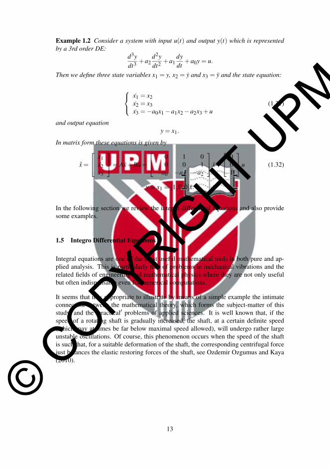
Then we define three state variables x1 = y, x2 = y and x3 = y and the state equation:

x1 = x2x2 = x3x3 =−a0x1−a1x2−a2x3 +u

(1.31)

and output equationy = x1.

In matrix form these equations is given by

˙x =

x1x2x3

= Ax+Bu =

0 1 00 0 1

−a0 −a1 −a2

x+

001

u (1.32)

y = x1 = [1,0,0]x.

In the following section we review the integro differential equations and also providesome examples.

1.5 Integro Differential Equations

Integral equations are one of the most useful mathematical tools in both pure and ap-plied analysis. This is particularly true of problems in mechanical vibrations and therelated fields of engineering and mathematical physics where they are not only usefulbut often indispensable even for numerical computations.

It seems that it is appropriate to illustrate by means of a simple example the intimateconnection between the mathematical theory, which forms the subject-matter of thisstudy, and the ′practical′ problems of applied sciences. It is well known that, if thespeed of a rotating shaft is gradually increased, the shaft, at a certain definite speed(which may at times be far below maximal speed allowed), will undergo rather largeunstable oscillations. Of course, this phenomenon occurs when the speed of the shaftis such that, for a suitable deformation of the shaft, the corresponding centrifugal forcejust balances the elastic restoring forces of the shaft, see Ozdemir Ozgumus and Kaya(2010).

13

© COPYRIG

HT UPM

In order to determine the possible ′critical′ speeds of the shaft, we may utilize a simple,yet general, result from the theory of elastic beams: For an arbitrary elastic beam underarbitrary end conditions, there always exists a uniquely defined influence function Gwhich yields the deflection of the beam in a given direction γ at an arbitrary point P ofthe beam caused by a unit loading in the direction γ at some other point Q. For, if thecross-sections of the beam are placed in one-to-one correspondence with the points ofthe segment 0 ≤ x ≤ 1, then G is a symmetric function G(x,y) of the abscissae x andy of P and Q respectively, see Yalcin et al. (2009). Consequently by the superpositionprinciple of elasticity, if p(x) is an arbitrary continuous load distribution along thebeams then the corresponding deflection is

z(x) =∫ 1

0G(x,y)µ (y)dy, (0≤ x≤ 1) (1.33)

This equation (1.33) is known as integral equation; more precisely, it is called a linearhomogeneous Fredholm equation of second kind with the kernel G(x,y)µ(y). If thekernel is complex or complicated we transform the kernel in different format. By us-ing the fact that µ(x) > 0 we can transform equation (1.33) into a similar one with asymmetric kernel that might be handle easy. For example, if we set

Φ(x) =√

µ (x)z(x) (1.34)

and ω2 = λ ,then we obtain the equation

Φ(x)−λ

∫ 1

0K (x,y)φ (y)dy = 0 (0≤ x≤ 1) (1.35)

whose kernelK(x,y) =

√[µ (x)µ (x)]G(x,y) (1.36)

is obviously symmetric.

Remark 1.5 The advantage of this transformation is that a symmetric kernel generallypossesses an infinity of eigenvalues ( also known as characteristic or proper values),i.e.values of λ for which the equation has non-zero solutions. On the other hand, a non-symmetric kernel may or may not have eigenvalues.

14

© COPYRIG

HT UPM

1.6 Objectives and Scope of the Study

This research consists of two parts. In the first part, we study the matrix differentialequations before and after convolutions as well as the effect on the solutions. In thesecond part, we solve integro differential equations by generating integro-differentialequations. Thus the main objectives of this research are summarized as follows:

(i) to provide the convolutions and existence of solutions to Volterra Equations,Volterra Integro-Differential Equations and some examples.

(ii) to study existence of the solutions of non-linear higher order boundary valueproblems using differential transformation method and convolution method.

(iii) to determine relations between differential equations and integro-differentialequations after convolutions.

(iv) to prove existence of solution for the type of integro-differential equations

and boundary values in the form of y(n)(x) =∫ t

0e−λ t ∗ (y(x− t))m dt and

y(n)(x) =∫ t

0p(t)∗ (y(x− t))m dt.

(v) to propose to solve singular integro - differential equations by smoothing on usingconvolution.

To verify the proposed theorems, the proofs are provided by using the standard provingtechniques. Some examples are provided to illustrate the proposed theorem.

15

© COPYRIG

HT UPM

1.7 Outline of Thesis

The thesis is divided into six chapters as follows.

Chapter 1 of this thesis is about introduction, necessary definitions, theorems, problemstatement and objectives.

Chapter 2 explains the literature review and the historical development of the study.

In Chapter 3, we provided the convolutions and existence of solutions such as VolterraEquations, Volterra Integro-Differential Equations and some related examples.

Chapter 4 is on the existence of the solutions of non-linear higher order boundary valueproblems using differential transformation method and convolution technique.

Chapter 5 is on the applications of the differential transformations to the non-linearhigher order matrix equations and also matrix equation systems.

Chapter 6 is on the future study and open problems.

16

© COPYRIG

HT UPM

BIBLIOGRAPHY

Abazari, R. and Kılıcman, A. (2012). Solution of second-order ivp and bvp of matrixdifferential models using matrix dtm. In Abstract and Applied Analysis, volume2012. Hindawi Publishing Corporation.

Anton, H., Bivens, I. C., and Single, S. D. C. E. T. (2009). Variable.

Arikoglu, A. and Ozkol, I. (2005). Solution of boundary value problems for integro-differential equations by using differential transform method. Applied Mathematicsand Computation, 168(2):1145–1158.

Arikoglu, A. and Ozkol, I. (2006). Solution of difference equations by using differentialtransform method. Applied Mathematics and Computation, 174(2):1216–1228.

Arikoglu, A. and Ozkol, I. (2007). Solution of fractional differential equations by usingdifferential transform method. Chaos, Solitons & Fractals, 34(5):1473–1481.

Ayaz, F. (2003). On the two-dimensional differential transform method. Applied Math-ematics and Computation, 143(2):361–374.

Ayaz, F. (2004). Solutions of the system of differential equations by differential trans-form method. Applied Mathematics and Computation, 147(2):547–567.

Borhanifar, A. and Abazari, R. (2010). Numerical study of nonlinear schrodinger andcoupled schrodinger equations by differential transformation method. Optics Com-munications, 283(10):2026–2031.

Borhanifar, A. and Abazari, R. (2011). Exact solutions for non-linear schrodinger equa-tions by differential transformation method. Journal of Applied Mathematics andComputing, 35(1):37–51.

Boyce, W. E., DiPrima, R. C., and Haines, C. W. (1969). Elementary differential equa-tions and boundary value problems, volume 9. Wiley New York.

Bracewell, R. N. and Bracewell, R. N. (1986). The Fourier transform and its applica-tions, volume 31999. McGraw-Hill New York.

Brychkov, I. A. (1992). Multidimensional integral transformations. CRC Press.

Che Hussin, C. H. and Kilicman, A. (2011). On the solutions of nonlinear higher-orderboundary value problems by using differential transformation method and adomiandecomposition method. Mathematical Problems in Engineering, 2011.

Che Hussin, C. H., Kilicman, A., Ishak, A., Hashim, I., Ismail, E. S., and Nazar, R.(2013). Solving system of linear differential equations by using differential trans-formation method. In AIP Conference Proceedings, volume 1522, pages 245–250.AIP.

Chen, C. and Liu, Y. (1998). Solution of two-point boundary-value problems usingthe differential transformation method. Journal of Optimization Theory and Appli-cations, 99(1):23–35.

92

© COPYRIG

HT UPM

Coddington, E. A. and Levinson, N. (1955). Theory of ordinary differential equations.Tata McGraw-Hill Education.

Davies, B. (2012). Integral transforms and their applications, volume 41. SpringerScience & Business Media.

Edwards, C. H. and Penney, D. E. (2004). Differential equations and boundary valueproblems, volume 2. Prentice Hall.

Eltayeb, H. and Kılıcman, A. (2008). A note on solutions of wave, laplaces and heatequations with convolution terms by using a double laplace transform. Applied Math-ematics Letters, 21(12):1324–1329.

Erturk, V. S. and Momani, S. (2007). Comparing numerical methods for solvingfourth-order boundary value problems. Applied Mathematics and Computation,188(2):1963–1968.

Folland, G. B. (1995). Introduction to partial differential equations. Princeton univer-sity press.

Hussin, C. H. C. and Kilicman, A. (2011). On the solution of fractional order nonlinearboundary value problems by using differential transformation method. EuropeanJournal of Pure and Applied Mathematics, 4(2):174–185.

Kilicman, A. (2001). A comparison on the commutative neutrix convolution of distri-butions and the exchange formula. Czechoslovak Mathematical Journal, 51(3):463–471.

Kılıcman, A. (2003). On the fresnel sine integral and the convolution. InternationalJournal of Mathematics and Mathematical Sciences, 2003(37):2327–2333.

Kılıcman, A. (2008). A remark on the products of distributions and semigroups. Jour-nal of Mathematical Sciences: Advances and Applications, 1(2):423–430.

Kilicman, A. and Al Zhour, Z. A. A. (2007). Kronecker operational matrices forfractional calculus and some applications. Applied Mathematics and Computation,187(1):250–265.

Kilicman, A. and Altun, O. (2011). On partial differential equations by using differen-tial transformation method with convolution terms. In 5th International Conferenceon Research in Education(ICREM 5). Journal of Metamathematical Analysis.

Kılıcman, A. and Altun, O. (2012). On the solutions of some boundary value prob-lems by using differential transformation method with convolution terms. Filomat,26(5):917–928.

Kilicman, A. and Altun, O. (2014). On higher-order boundary value problems by usingdifferential transformation method with convolution terms. Journal of the FranklinInstitute, 351(2):631–642.

Kilicman, A. and Ariffin, M. K. (2002). Distributions and mellin transform. Abstractand Applied Analysis, 25:93–100.

93

© COPYRIG

HT UPM

Kilicman, A., Atan, K., and Eltayeb, H. (2011). A note on the comparison be-tween laplace and sumudu transforms. Bulletin of the Iranian Mathematical Society,37:131–141.

Kılıcman, A. and Eltayeb, H. (2009). A note on defining singular integral as distri-bution and partial differential equations with convolution term. Mathematical andComputer Modelling, 49(1):327–336.

Kılıcman, A. and Eltayeb, H. (2011). On finite products of convolutions and classifica-tions of hyperbolic and elliptic equations. Mathematical and Computer Modelling,54(9):2211–2219.

Kılıcman, A. and Eltayeb, H. (2012). Note on partial differential equations with non-constant coefficients and convolution method. Appl. Math, 6(1):59–63.

Kilicman, A., Eltayeb, H., and Agarwal, R. P. (2010). On sumudu transform and sys-tem of differential equations. In Abstract and Applied Analysis. Hindawi PublishingCorporation.

Kilicman, A. and Gadain, H. E. (2009). An application of double laplace transform anddouble sumudu transform. Lobachevskii Journal of Mathematics, 30(3):214–223.

Kilicman, A. and Gadain, H. E. (2010). A note on integral transforms and partialdifferential equations. Applied Mathematical Sciences, 4(3):109–118.

Lewy, H. (1957). An example of a smooth linear partial differential equation withoutsolution. Annals of Mathematics, pages 155–158.

Long, N. T. and Dinh, A. P. N. (1995). Periodic solutions of a nonlinear parabolic equa-tion associated with the penetration of a magnetic field into a substance. Computers& Mathematics with Applications, 30(1):63–78.

Neta, B. and Igwe, J. O. (1985). Finite differences versus finite elements for solv-ing nonlinear integro-differential equations. Journal of mathematical analysis andapplications, 112(2):607–618.

Ozdemir Ozgumus, O. and Kaya, M. (2010). Vibration analysis of a rotating taperedtimoshenko beam using dtm. Meccanica, 45(1):33–42.

Rahman, M. (2007). Integral equations and their applications. WIT press.

Ross, B. (2006). Fractional calculus and its applications: proceedings of the inter-national conference held at the University of New Haven, June 1974, volume 457.Springer.

Sumita, U. (1984). The matrix laguerre transform. Applied Mathematics and Compu-tation, 15(1):1–28.

Tari, A. (2012). The differential transform method for solving the model describingbiological species living together. Iranian Journal of Mathematical Sciences andInformatics, 7(2):63–74.

Tricomi, F. G. (1985). Integral Equations. Dover Publications; Revised ed.

94

© COPYRIG

HT UPM

Wazwaz, A.-M. (2000). Approximate solutions to boundary value problems of higherorder by the modified decomposition method. Computers & Mathematics with Ap-plications, 40(6-7):679–691.

Wazwaz, A.-M. (2001). The numerical solution of fifth-order boundary value problemsby the decomposition method. Journal of Computational and Applied Mathematics,136(1):259–270.

Xie, M. and Ding, X. (2011). A new method for a generalized hirota–satsuma coupledkdv equation. Applied Mathematics and Computation, 217(17):7117–7125.

Yalcin, H. S., Arikoglu, A., and Ozkol, I. (2009). Free vibration analysis of circularplates by differential transformation method. Applied Mathematics and Computa-tion, 212(2):377–386.

Zhou, J. (1986). Differential transformation and its applications for electrical circuits.

Zuidwijk, R. (1996). M. holschneider, wavelets: An analysis tool.

95

© COPYRIG

HT UPM

BIODATA OF STUDENT

Omer Altun was born in Tokat, Turkey. He finished elementary school and primaryschool in Erbaa, high secondary school in Unye. He joined the Department of Mathe-matics, Faculty of Education, Ataturk University and awarded the of Bachelor of Math-ematics in 2008. He graduated from University of Putra, Malaysia in 2012 with aMaster of Science in Mathematics in the field of Functional Analysis. He enrolledthe PhD programme in University Putra Malaysia, Faculty of Science, Department ofMathematics in 2012. He has completed the PhD in 2016.

His research area interests are differential transformation method, ordinary differentialequation, boundary value problem and convolutions. During his PhD candidature, hesubmitted several papers to journals and some of them published and some still waitingfor publications. He also attended several conferences overseas as a speaker to enrichhis knowledge and to gain experiences.

99

© COPYRIG

HT UPM

LIST OF PUBLICATIONS

Kılıcman, Adem; Altun, Omer. On the solutions of some boundary value problemsby using differential transformation method with convolution terms. Filomat 26(2012), no. 5, 917–928. MR3098737.

Kılıcman, Adem; Altun, Omer. On higher-order boundary value problems by usingdifferential transformation method with convolution terms. J. Franklin Inst. 351(2014), no. 2, 631–642. MR3151777 (Reviewed).

Kılıcman, Adem; Altun, Omer. Some remarks on the fractional Sumudu transformand applications. Appl. Math. Inf. Sci. 8 (2014), no. 6, 2881–2888. MR3228687.

Omer Altun and Adem Kılıcman. On solutions of matrix initial value problems byusing differential transform method and convolution, AIP Conf. Proc. 1557, 191(2013); http://dx.doi.org/10.1063/1.4823901 Conference date: 57 February 2013,Location: Kuala Lumpur, Malaysia

Omer Altun and Adem Kılıcman. On Partial Differential Equations by Using differ-ential Transformation method with Convolution terms, Presented during the 5th

International Conference on Research in Education and Mathematics (ICREM 5),22-24th October 2011, Bandung, Indonesia.

Omer Altun and Adem Kılıcman. On solution of higher order nonlinear matrixvalue problems by using differential transformation method and convolutions, pre-sented during the International conference and Workshop on Mathematical Analy-sis(ICWOMA 2014), 27th-30th May 2014, Putrajaya, Malaysia

Omer Altun and Adem Kılıcman. On convolution, Singularities and Fractional Dif-ferential and Integro-Differential Equations, presented during the 2nd InternationalConference on Mathematical Sciences and Statistics(ICMSS 2016), 26th-28th Jan-uary 2016, Kuala Lumpur, Malaysia

100

© COPYRIG

HT UPMUNIVERSITI PUTRA MALAYSIA

STATUS CONFIRMATION FOR THESIS/PROJECT REPORT AND COPYRIGHTACADEMIC SESSION: Second Semester 2016/2017

TITLE OF THE THESIS/PROJECT REPORT:SOLVING MATRIX DIFFERENTIAL AND INTEGRO-DIFFERENTIAL EQUATIONS BY

USING DIFFERENTIAL TRANSFORMATION METHOD AND CONVOLUTIONS

NAME OF STUDENT: OMER ALTUN

I acknowledge that the copyright and other intellectual property in the thesis/project report be-longed to Universiti Putra Malaysia and I agree to allow this thesis/project report to be placed atthe library under the following terms:

1. This thesis/project report is the property of Universiti Putra Malaysia.

2. The library of Universiti Putra Malaysia has the right to make copies for educationalpurposes only.

3. The library of Universiti Putra Malaysia is allowed to make copies of this thesis for aca-demic exchange.

I declare that this thesis is classified as:

*Please tick(X)� � CONFIDENTIAL (contain confidential information under Official Secret

Act 1972).� � RESTRICTED (Contains restricted information as specified by the

organization/institution where research was done).� � OPEN ACCESS I agree that my thesis/project report to be published

as hard copy or online open acces.This thesis is submitted for:� � PATENT Embargo from until .

(date) (date)Approved by:

(Signature of Student) (Signature of Chairman of Supervisory Committee)New IC No/Passport No.:U05604460 Name: Professor. Dr. Adem Kılıcman, PhD

Date: Date:

[Note: If the thesis is CONFIDENTIAL or RESTRICTED, please attach with the letterfrom the organization/institution with period and reasons for confidentially or restricted.]