2016 Online Competition

Guidelines

Student teams will have a total of one week to complete the exam from start to finish. There are twoseparate sections for this examination: one section on Laser and Plasma Physics, and one section on Entropyand Statistical Mechanics. Teams may complete both sections or choose to complete only one, as is specifiedin the grading explanation below. We recommend that teams set aside approximately 20+ hours to allowenough time for successful completion. Please refer to the submission explanation below for details on bothformatting and the submission process.

Grading

Students are encouraged to work on as much of both sections of the exam as possible. However, teamsmay choose to submit solutions for only one of the two sections if they desire. The two sections willbe graded separately, and may not necessarily be worth the same amount of points. The award structurewill be as follows:

1. Awards will be given to the four teams with the highest score in each section (an award for firstplace, second place, third place, and fourth place). One team can win an award for both sections, suchas second place in Laser and Plasma Physics and fourth place in Entropy and Statistical Mechanics.Therefore teams are encouraged to attempt solutions for both sections of the competition.

2. We will additionally award one overall award to the highest scoring team on the entire com-petition. A team which wins this overall award can still receive one of the top four awards for eachindividual section. The team that wins this overall award will most likely have completed both sectionsof the exam. It will be at the judges’ discretion to choose the overall award for the best submission.

3. Special awards will also be given for honorable mentions, the most elegant solution, and the mostcreative solution.

Collaboration Policy and Resources

Students participating in the competition may only correspond with other members of their team. Noother human correspondence is allowed, including: mentors, teachers, professors, and other students. Ingeneral, participating students are barred from posting content or asking questions related to the exam onthe internet (except where specified below). Students are, however, allowed to use the following resources:

• Online: Teams may use any information they find useful on the Internet. However, under no circum-stances may they actively post content or ask questions about the exam.

• Piazza page: Teams are encouraged to create an account on Piazza and register in the class atthe following URL: http://piazza.com/princeton_university_physics_competition/fall2016/pupc2016. The access code is: pupc2016. This resource can be used by teams to ask questions aboutthe content of the exam. Please do not post any of your solutions, partial or complete, when askingquestions on Piazza.

1

• Published Materials: Teams may take advantage of any published material, both printed or online.

• Computational: Teams may use any computational resources they might find helpful, such as Wol-fram Alpha/Mathematica, Matlab, Excel, or lower level programming languages (C++, Java, Python,etc). For some sections, the use of computational resources is highly advised.

Citations

All student submissions with outside material must include numbered citations. We do not prefer anystyle of citation in particular. Students may find the following guide useful in learning when to cite sourcedmaterial: http://www.princeton.edu/pr/pub/integrity/pages/cite/.

Submission

All submissions, regardless of formatting, should include a cover page listing the title of their work,the date, and signatures of all team participants. The work must be submitted as one singlePDF document with the “.pdf.” extension. All other formatting decisions are delegated to theteams themselves. No one style is favored over another. That being said, we recommend that teams use atypesetting language (e.g., LATEX) or a word-processing program (e.g. Microsoft Word, Pages). Handwrittensolutions are allowed. Note: we reserve the right to refuse grading of any portion of a team’ssubmission in the case that the writing or solution is illegible.

Teams must submit their Online Part solutions by e-mailing pupc@princeton.edu by 11:59 am (noon)Eastern Time (UTC-5) on Saturday, November 19, 2016. Teams will not be able to submit their solutions tothe Online Part at any later time. Any team member may send the submission. The title of the submission e-mail should be formatted as “SUBMISSION - Team Name”. Note: all teams may make multiple submissions;however, we will only grade the most recent submission submitted before the deadline. Teams will receiveconfirmation once their submission has been received within at most two days. In the case ofextraordinary circumstances, please contact us as soon as possible.

Sponsors

Collaborators

2

Entropy and Statistical Mechanics Section

The subject matter of this document is statistical mechanics, or the study of how macroscopic resultsmanifest from microscopic interactions in systems with many interacting parts.

Our goal is to provide a unified introduction to statistical mechanics using the concept of entropy. Aprecise definition of entropy pervades statistical mechanics and other scientific subjects and is useful inits own right. While many students may have heard the word entropy before, entropy is rarely explainedin its full detail or with rigorous mathematics, leaving students confused about many of its implications.Moreover, when students learn about thermodynamic laws, laws that describe the macroscopic results ofstatistical mechanics, like “change in internal energy = heat flow in + work done on a system”, the conceptsof internal energy, heat, and work are all left at the mercy of a student’s vague, intuitive understanding.

In this document, we will see that formulating statistical mechanics with a focus on entropy can providea more unified and symmetric understanding of many of the laws of thermodynamics. Indeed some laws ofthermodynamics which appear confusing and potentially unrelated at first glance can in fact all be seen tofollow from the same treatment of entropy in statistical mechanics.

Contents

1 Entropy as information 51.1 Quantifying the amount of information in the answer to a question . . . . . . . . . . . . . . . 5

2 Where does entropy show up in Statistical Mechanics? 72.1 An example: rigid chain and the “force” that entropy causes . . . . . . . . . . . . . . . . . . 82.2 An abstract derivation of entropy in statistical mechanics . . . . . . . . . . . . . . . . . . . . 102.3 Why is our definition of temperature reasonable? . . . . . . . . . . . . . . . . . . . . . . . . . 132.4 Extensions of the conceptual model . . . . . . . . . . . . . . . . . . . . . . . . . . . . . . . . . 15

3 A more precise analysis of free energy and entropy 163.1 A system coupled to an energy reservoir . . . . . . . . . . . . . . . . . . . . . . . . . . . . . . 163.2 A system coupled to an arbitrary reservoir . . . . . . . . . . . . . . . . . . . . . . . . . . . . . 193.3 Summary of generalized analysis of free energy and work done on a system . . . . . . . . . . 23

4 Applications: non-equilibrium changes in biological and computational systems 244.1 Jarzynski’s equality: a non-equilibrium work relation . . . . . . . . . . . . . . . . . . . . . . . 254.2 Dissipation in computational systems . . . . . . . . . . . . . . . . . . . . . . . . . . . . . . . . 27

Learning goals of this topic: This topic is meant as an exercise in learning more so than an exercise insolving problems or external research. The goal of this topic is for the reader, who has not necessarily seenany statistical mechanics in their education so far, to walk away with a set of examples and ideas that willbe helpful long into the future.

Topic format: This document consists of long sections of explanatory material with helpful exercises andquestions interspersed. Much of the grading will be based on sections that ask you to explain or interpretresults in your own words. We are looking to see how well you understand the subject, and are not overlyconcerned with minor errors in completing exercises.

Expected amount of work: Do not expect to understand the concepts in this document after only oneread through. These topics take time to absorb. While it may feel like you are not getting much accomplishedas you try to understand the reading, we expect that it may be necessary to read some passages four timesin a row before understanding it completely. Because there are not too many questions in this document,you should have time to complete the readings.

3

Many pages of this document have only one or two places where the author asks for input and responsefrom the readers. Some sections contain no questions. We would encourage you not to skip reading thesesections completely, as all sections of this document will be beneficial to understand.

Additional reading materials and resources

While this document is meant to generally stand alone as an explanation of entropy, free energy, andrelated concepts, you may find a few outside sets of information useful:

• Required reading:

– Equilibrium Information from Nonequilibrium Measurements in an ExperimentalTest of Jarzynski’s Equality, J. Liphardt et al., Science 296, 5574 (2002): this paper experi-mentally verifies the results of the above paper by C. Jarzynski. It is explored in detail in Section4.1.2.

• Additional potential resources:

– Thermal Physics by Charles Kittel and Herbert Kroemer (1980, W. H. Freeman and Company):an extensive introduction to concepts discussed within this document. While this reference maybe useful for clarifications of certain concepts, it is not at all essential.

– Nonequilibrium Equality for Free Energy Differences, C. Jarzynski, Phys. Rev. Lett. 78,2690 (1997): this reference is discussed in Section 4.1 of this document as an application of thetheoretical results derived herein.

– Feynman Lectures on Computation by Richard Feynman, edited by Tony Hey and RobinW. Allen (1996, Perseus Publishing): this reference is an interesting book which contains manyuseful and intuitive explanations of statistical applications in computing. Of particular interestfor this document is the chapter on reversible computation. This reading is relevant to Section4.2, all though it is by no means necessary to complete the questions in that section.

4

1 Entropy as information

At this point in your life, you may have heard the word entropy, but chances are, it was given a vague,non-committal definition. The goal of this section is to introduce a more explicit concept of entropy froman abstract standpoint before considering its experimental and observational signatures.

1.1 Quantifying the amount of information in the answer to a question

Entropy, while useful in physics, also has applications in computer science and information theory. Thissection will explore the concept of information entropy as an abstract object.1

We will first consider entropy not as related to the concept of heat in objects, but as a purely axiomaticquantification of what we mean by the information we receive when we hear the answer to a question. Fora concrete example, imagine that someone flips a coin and doesn’t reveal which side landed upright and weask “what was the outcome of the coin flip? Heads or tails?” When they now tell us the answer, how much“information” do we gain by learning what the outcome was? In other words, we are faced with determininghow much information is received when we hear the answer to a question that has a probability distributionof outcomes. This question was asked by Claude Shannon in 1948.

After pondering this question for a long time, you might come up with a few criteria that any reasonablemeasure must obey, such as:

1. If the question has two answers that are not dependent on each other, then the measure of informationcontained in answering both questions should be the same as the sum of the information gained inlearning the answer to each one individually.

For example, if we have two independent coin flip experiments, the information gained in hearing theoutcome of one coin flip should be the same as the information gained in hearing the outcome of theother, so that the total information gained is the sum of the individual amounts of information gained.

How does this concept generalize to questions which have interdependent answers? Two such questionsmight be “am I wearing gloves?” and “am I wearing a sweater?”. The exact statement of this criteriais more complicated and we will not ask you to consider it here.

2. The measure of the information learned should not depend on the language used; it should dependonly on the probability distribution of possible answers.

For example, it should not depend on the fact that we are flipping a coin and asking whether it is headsor tails instead of flipping a dinner plate and asking if it lands upright or not. The measure of theinformation gained should be the same. For this reason, the measure should depend on the probabilitydistribution of answers to the question, not the content of the answers.

3. The information gained should be largest when all possible answers are equally likely.

If we have no idea which answer it will be, we will gain the most information possible when we hearan answer. For example, if a fair dice with 6 sides is rolled, it has an equal chance of landing on eachside, and you gain the most information possible by learning which side the dice landed on. On theother hand, if the dice was unfair and landed on a specific side every time, then you learn no newinformation by learning the outcome of the dice role; you already knew what it would be before yourolled the dice.

While there are other possible additional criteria to use when defining the information gained by hearing theanswer to a question, these are sufficient for our purposes in this document.

Now, for a definition: given a probability distribution of possible outcomes (such as answers to a question)with associated probabilities pi for each outcome, the logical quantification of the average information gainedif one outcome is obtained (if we learn the answer to a question) is the Information Entropy I,

I =

N∑i=1

pi log(1/pi) = −N∑i=1

pi log(pi). (1)

1The author would like to acknowledge that some of the writing in this section is based on information from a class instatistical mechanics taught by Prof. William Bialek at Princeton University.

5

Questions Explore this definition of information entropy for a few example probability distributions overa finite set of outcomes (such as 2 or 4) and summarize your findings. Note that log(x) refers to the naturallogarithm of x (base e, not base 10 or base 2), and will refer to the natural logarithm throughout thisdocument. Is this quantity always positive (despite the minus sign in the definition)? For a fixed numberof possible outcomes, N , but varying probabilities pi, what is the range of possible values that I can take(the maximum minus the minimum)? What is the minimum amount of information you can learn from theanswer to a question, in words, and why? A simple example to begin with is the probability distributionof a coin toss, where pheads = 1/2 and ptails = 1/2. What happens if you measure the logarithm with adifferent base (such as base 10 instead of the natural logarithm)? This is related to the concept of measuringinformation with different scales, just as we can measure a mass as 1 kilogram or as 1000 grams. Now, goback and consider the definition of information entropy with respect to the criteria listed above. Does thisdefinition of entropy satisfy criteria 1, 2, and 3? (Ignore the case of interdependent answers in criterion 1.)

6

2 Where does entropy show up in Statistical Mechanics?

We will now consider how entropy relates to physics. This section contains no questions for the reader.Consider a glass of water. At any given moment, if you were to look at a snapshot of all the atoms of

water in the glass, there would be an unimaginably large number of arrangements these atoms could be in.Statistical mechanics on some level requires us to admit that we are not all knowing beings, and cannotalways tell if the system is in one configuration or another. In effect, we assume that we could never knowthe location of all of these molecules at one time, and as such we can only ask other types of questions.This is where entropy shows up. Now, we ask “what is the configuration of atoms in the glass of water?”The set of possible outcomes is the set of all possible positions of all the atoms. This is a large set, and wewould not hope to actually be able to calculate the information entropy of the system by finding each piand computing the information entropy I. On the other hand, the abstract language of mathematics lets usengage with this problem regardless of our gaps in knowledge. Even if we do not know all of the pi, theystill exist, and so the entropy of this question still exists and is not meaningless to talk about.

Let us consider a simpler picture. Various symbols will be introduced to define quantities. Do not beintimidated, but rather read slowly to absorb the information. We define Ω (capital omega) as the set ofall possible outcomes ωi (lowercase omega) for the configuration of atoms in the glass, indexed by a numberi. That is, the set Ω = ω1, ω2, . . . , ω9, ω10 would describe a situation with 10 possible outcomes, and sowith 10 elements.2 These 10 outcomes are the possible configurations of atoms in the glass. It may be hardto imagine some set of atoms having only a finite number of possible configurations, rather than an infinitenumber, but for now assume that it is true. If we as physicists have not discovered energy or any othervariable that might make one outcome more likely than any other (people usually say lower energy states aremore likely, and we will see why), we could expect that each outcome ωi is equally likely. That is, pi = 1/10for all i. This seems rather simple, and it is reasonable to question why it would be true that each pi = 1/10.For now, assume it is true. We could immediately ask what is the information entropy in the question “whatis the state of the water glass?” In this case, I = log(10).

However, we are not always interested in what the state of the system, is, but rather some other property,such as how high the water in the glass is. If each outcome ωi has a different value for the height of thewater, the situation is more complicated, and the question “what is the height of the water in the glass”would have a different information entropy than the question “what is the state of the system?”.

As a concrete example, let us say that 4 of the ωi have a height 5 cm, 3 have a height 3 cm and 3 havea height 2 cm. Now, the question, “what is the height of the water’?’ has a less well defined answer. Wecan compute the expected height we would see on average (given the probability of each ωi). This is h =∑i pihi = (4 × 5 + 3 × 3 + 3 × 2)/10 cm = 3.5 cm. We can also compute the information entropy of the

question. The information entropy, I, is given by

I =2

5log

(5

2

)+

3

10log

(10

3

)+

1

5log

(5

1

)≈ 1.0495.

Note that this information entropy is different from the value log(10) ≈ 2.3026 for the entropy of the stateof the system. Therefore, you must be careful about what questions you are asking and answering whencomputing information entropy.3 Both the average height and the information entropy tell us somethingdifferent about the answer to the question “what is the height of the water?”

Much of statistical mechanics follows this same vein of reasoning: we assume some set of states of thesystem are equally likely, but then we ask something about a property that varies across the states (likeenergy, or the height of water). What ends up mattering for this secondary question is how many statesthere are with a certain property. Ultimately, entropy is intimately related to how we understand and thinkabout answers to these questions.

2In general, Ω could have N elements, where N could be as large as 1023!, a very large number.3It is also useful to note that the information entropy is not telling us something about how precisely we know the height of

the water. The information entropy I would have the same value if the three possible heights were 1 cm, 1.0001 cm, and 58476cm, for example.

7

2.1 An example: rigid chain and the “force” that entropy causes

We will now consider a more concrete example system than a glass of water molecules and how entropyinforms our understanding of this system.4

2.1.1 A description of the physical model

Consider a chain that is made up of N rigid straight sections connected to each other at bendable hinges.Assume that one end of the chain is fixed at position x = 0, while the other is free to move around.

We will make one other crucial assumption which may not make intuitive sense. For the purpose of thisexample, assume that the states of the chain that we observe are always with the entire chain confined toone dimension, the x axis. This means that the bends at each hinge are always 0 or 180 (0 or π radians),and the chain can double back on itself any number of times. We will assume that there is some way forthe system to go from a bend being 0 to 180, but we do not care what it is at this point. Examples of thefour possible configurations of a rigid chain with two segments are shown in Fig. 1.

Figure 1: Diagram of the four possible configurations of a rigid chain with two segments. The chain isconfined to lie in one dimension and the end of the chain designated by the blue dot is held fixed at x = 0.

We will further assume that each segment of the chain has length 1/2 (in some units). We will alsoassume that N is an even number so that the location of the free end of the chain is at a position x that isan integer (because each segment of the chain has length 1/2). This choice is not important, but will makecalculations easier. For this reason, a chain with two segments can have its end position lie at x = −1, x = 0,or x = 1, as is shown in Fig. 1.

2.1.2 Finding the probability of certain positions

Like before, we assume that all configurations of the chain are equally likely, meaning the chain has nopreference for whether a hinge is straight or bent at 180.

Questions Now, what is the probability distribution of the location of the free end of the chain if allconfigurations of the chain are equally likely? There are multiple ways of finding this answer, but for now,try to follow this “chain” of reasoning:

1. List all possible locations of the free end of the chain.

2. List the number of possible configurations of a single link in the chain. Now, what is the number ofpossible configurations for the entire chain all at once? (We are asking how many outcomes for the

4The author would like to acknowledge that this example is based on information from a class in statistical mechanics taughtby Prof. William Bialek at Princeton University.

8

chain configuration are possible, not how many locations. This is the analogous question to the aboveexample of a cup filled with water. We are not asking how many possible heights of the water in theglass there are, but rather how many possible states there are.).

3. For a given −N/2 ≤ n ≤ N/2, how many ways can the free end lie at position x = n? (Hint: considerthe case of a small chain first and see if you can work your way up to a general expression involvingfactorials, where m factorial is m! = (m)(m− 1)(m− 2) · · · (2)(1).)

4. If all of these individual configurations of the chain are equally likely (meaning any given configurationof hinges being bent or not bent), then what is the the probability p(x = n) that the chain position xis given by a specific value of n for |n| ≤ N/2?

You should now have some grasp of what a likely position of the end of the chain is.

Note that the most likely locations of the end of the chain are the locations for which the most numberof states of the system have that location. This idea in fact relates back to our idea of entropy; if you weretold that the end of the chain was actually at a certain value of x = n, but that all states which producedthis end of chain location were equally likely, you could compute the information entropy of the question“what is the state of the system given that x = n?”. For clarity, we can define this information entropy asσSys(x = n). In some sense, you have already done the necessary work to compute σSys(x = n)) in the abovesteps. Write down a formula for σSys(x = n) explicitly.

Next, write down a formula relating p(x = n) to σSys(x = n) for the same n. Note that larger values ofσSys(x = n) relate directly to larger values of p(x = n).

2.1.3 Stirling’s approximation: a way to simplify the formula

Now we shall engage in a classic past-time of physicists: approximation. We will use the fact that n! isapproximately given by

n! ∼√

2πn(ne

)n(2)

when n is large. This equation is known as Stirling’s approximation. Elementary explanations of why thisis true can be found online if you are intrigued, as well as qualifications of its validity.

Questions Now, derive an approximate expression for p(x = n) that is simpler than the one you foundbefore by using Stirling’s approximation. You may also find it useful to know that

ex = limm→∞

(1 +

x

m

)m.

We shall refer to this approximate probability formula that you find as ps(x = n), and it is not the exactvalue of the probability that x = n, although it is extremely close in most cases and makes some of theresulting physics clearer. You should obtain, with sufficient approximation, a proportionality of

ps(x = n) ∝ 1√N

exp

(−4x2

N

).

(The symbol ∝ means “is proportional to” up to a constant factor. The notation “exp(x)” means ex. Ifyou do not get precisely the same answer, this is alright, just show your work. The factor of −x2 in theexponential is what is important.) Stirling’s approximation is important because it allows us to make senseof the behavior of the system when N is large and when the exact formula is not particularly enlightening.

In particular, with our result for ps(x = n), we can find an expression for σSys(x = n) which is mucheasier to work with. Use our formula relating p(x = n) to σSys(x = n) for the same n that we derived aboveto find a simpler expression for σSys(x = n).

9

2.1.4 An aside on energy vs. entropy

One of the important results of thermodynamics is that, for an abstract system exchanging energy withan energy reservoir, the probability of observing any state ωi of the system is proportional to exp(−E(ωi)/τ).The reservoir is simply a collection of objects with a large energy that can exchange that energy in some waywith the abstract system. The quantity E(ωi) is the energy of state ωi and τ is a property of the reservoircalled temperature. We will discuss this in more detail in Section 2.2.

Now, consider a 1 dimensional spring with spring constant k and equilibrium extension 0 that exchangesenergy with a reservoir somehow. The probability of observing an extension to a length x would be propor-tional to exp(−(1/2)kx2/τ).

In some sense, we can make an analogy between the rigid chain and this 1 dimensional spring. In thecase of the rigid chain, the negative of the entropy, or −σSys(x = n), plays the role of an “energy”, andhigher values of −σSys(x = n) lead to an exponentially suppressed probability of observing that value ofx. Taking the analogy further, −σSys(x = n) changes approximately as (1/2)kx2, which is similar to thepotential energy of an extended spring. In the end, the system behaves nearly identically to a 1 dimensionalspring exchanging energy with a bath. However, the potential energy of the analogous “spring” arises onlyfrom the entropy of the system, not from any real spring forces.

Summary The above discussion was meant to provide an intuition that entropy well and truly matters fora system such as the rigid chain. Now, it remains to be seen whether my interpretation of entropy acting likea spring restoring force has any validity (you should of course be skeptical of this rather contrived example).

2.2 An abstract derivation of entropy in statistical mechanics

Now that we have considered a specific example with an intuitive exhibition of how entropy appears ina mechanical system, we will consider a more general application of entropy in statistical systems.

2.2.1 Definitions

Consider an abstract system and reservoir (think of a small object like a glass of water and the roomaround it). The system S and reservoir R each have possible outcomes ωSi and ωRj where i and j range over

some set of integers. However, we can consider their outcomes jointly, as possible outcomes ωS,Ri,j defined to

be ωS,Ri,j = ωSi , ωRj , meaning that S is in state i and R is in state j at the same time. Now, let us consideranother quality of the system. We will call it energy, but what it really is doesn’t matter to us yet. Let usassume that the total energy Etot = ERes + ESys is conserved and therefore doesn’t change in time (again,this is just an assumption). We may not know the exact value, but it is conserved nonetheless. Let us now

make the assumption that all possible outcomes ωS,Ri,j are equally likely, as long as they have the correct total

energy. Thus we have the two assumptions:5

1. All possible states for the combined system and reservoir ωS,Ri,j must have the correct total energy.

This assumption should be somewhat familiar to physics students, and follows from the fact that energyis conserved globally, and that we assume the system and reservoir together are isolated from anythingelse in the universe.

2. All states for the combined system and reservoir that have the correct total energy are equally likely tobe observed.

Why are all states that have the correct total energy equally likely? To intuitively describe why, weneed to change how we think about this physical situation. In a classical system (in the case where

we ignore quantum mechanics), the system really is in one single state ωS,Ri,j at a given instant intime. However, because of natural interactions, this state will change over time. In some cases, we can

5There are additional assumptions we are making, of course, but they are a little more subtle and less relevant to the pointhere. On some level, stating that we can distinguish the energy of the system from the energy of the reservoir, and the statesof the system from the states of the reservoir, requires us to assume that there are not strong interaction energies between thesystem and reservoir. This is not a relevant detail at our level of analysis here, however.

10

assume that the system and reservoir will visit every possible state ωS,Rk,l over time, and that the systemand reservoir will spend roughly the same amount of time in each state as the state cycles through allavailable states. As long as the changes between states occur very quickly compared to the timescalebetween when we observe the system, then effectively we are just as likely to observe any one of thestates as any other. This is roughly the physical picture of why each state of the combined system andreservoir with the correct total energy is equally likely to be observed.6 This is basically a statementthat we are as maximally confused as possible about everything about the system, except that totalenergy is conserved.

These are not the only assumptions we will make in the course of our analysis, but they are the importantones for now. It is important to keep track of additional assumptions we will make. We will now endeavorto see what these assumptions imply about the likelihood of various states of the system.

2.2.2 A derivation

Having established the necessary notation, we will consider how likely it is for a certain state ωSk to be

observed which has energy Ek. Because all states ωS,Ri,j are equally likely, the probability of observing ωSk is

the number of states of the reservoir that can exist in a combination with ωSk , divided by the total numberof available states of the combined system and reservoir. This is just the usual formula for the probabilityfor event A to occur (a state ωSk of the system to be observed); it is the number of ways event A can occur(the number of states of the combined system and reservoir which have the system in state ωSk ) divided bythe total number of possible events (the number of all possible states of the combined system and reservoir).States of the reservoir, ωRj , that can pair with ωSk must have Ej = Etot−Ek because of the requirement thatthe energy of the combined system is Etot. The number of states of the reservoir with energy Etot −Ek willvary as a function of Ek. Indeed, we can define exp(σRes(E)) as the number of states of the reservoir whichhave energy E. In this way, the function σRes(E) represents the logarithm of a specific number of states ofthe reservoir. This should remind you of the entropy of a question with many, equally-likely answers.

Explicitly, the probability of observing a state ωSk of the system with energy Ek is given by

p(ωSk ) =exp(σRes(Etot − Ek))

ζ1, (3)

where ζ1 (the Greek letter “zeta”) is just a normalization constant that depends on the total number ofoutcomes possible for the combined system and reservoir, and ensures the total probability is 1. We can nowdefine something called temperature τ (we will discuss its physical meaning later), to be given by7

1

τ≡ β ≡ ∂σRes(E)

∂E

∣∣∣∣E=Etot

. (4)

If we can assume that σRes(Etot−Ek) is only slightly altered from σRes(Etot), then to a good approximationσRes(Etot − Ek) = σRes(Etot)− βEk, with β being the constant inverse temperature defined above, and

p(ωSk ) =eσRes(Etot)

ζ1exp(−βEk) =

1

ζ2exp

(−Ekτ

), (5)

where we have used the fact that exp(σRes(Etot)) is a constant and we have defined ζ2 as another normal-ization constant. The above formula is extremely important and its derivation should be well understoodbecause similar ideas and derivations will be used throughout this document.

One objection you may have to the above argument is whether we can truly consider temperature (asdefined here) to be fixed in some physical systems independent of Ek, or in other words you may wonderwhat the degree of error is in the statement that σRes(Etot − Ek) = σRes(Etot)− βEk. In general, what we

6This physical pictures is further explained in Section 4.0.1.7Note that ≡ is shorthand for “is defined to be”, as opposed to simply “equals”.

11

are really doing here, if you have a background in Calculus, is Taylor expanding σRes(Etot − Ek) close toσRes(Etot). First we write

σRes(Etot − Ek) = σRes

(Etot

(1− Ek

Etot

)).

Next, to be concise, define εk ≡ Ek/Etot. Then by Taylor expanding we have

σRes(Etot − Ek) = σRes(Etot) + (−εk)Etot∂σRes(E)

∂E

∣∣∣∣E=Etot

+ (−εk)2 1

2!(Etot)

2 ∂2σRes(E)

∂2E

∣∣∣∣E=Etot

+ · · · .

In the event that Ek is “small enough” so that εk = Ek/Etot 1, then only keeping terms in the Taylorexpansion to first order in εk (the first two terms on the right hand side of the “=” sign) accurately describesthe value σRes(Etot − Ek). For a fixed Etot, this just requires that Ek is made small enough.

Questions If we now consider the probability of observing a certain energy rather than a certain state forthe system, what is the new formula for p(ESys = Ek)? If there are exp(σSys(E)) number of states of thesystem at energy E, prove that

p(ESys = Ek) =1

ζ3exp(−β(Ek − τσSys(Ek)) =

1

ζ3exp(−βF(Ek)) (6)

for some constant ζ3. Here we have defined a function called the Free Energy F(Ek) = Ek − τσSys(Ek)as a function of Ek. This formula for p(ESys = Ek) should be reminiscent of the bendable chain examplederived earlier.

Note that the most likely energy of the system to be observed is the one which results in the lowest valueof F(Ek), and this energy is not necessarily the lowest possible value of energy. Can you describe in wordswhy this is true? What two effects are “competing” to determine the most likely state?

2.2.3 Clarifying types of entropy

As a clarification, I want to mention that we need to keep straight a few of the different entropies thatwe are considering. As was discussed above, the entropy of a system is equivalent to the information entropyof the question “what is the state?” Clearly, this has different meanings if we are talking about the stateof the combined system and reservoir, or if we are talking about the state of the system alone, or if we aretalking about the state of the system when we are at a fixed energy. Below is a list of the various entropieswe have been considering and their distinctions.

1. Entropy of the state of the combined system and reservoir:

This is the entropy of the question “what is the state of the combined system and reservoir?” Whilethis entropy is generally not considered in this document (it is not particularly useful), you shouldknow what it is. It depends only on the size of the set of all possible outcomes of the combined systemand reservoir, or ωS,Ri,j .

2. Entropy of the state of the system:

This is the entropy of the question “what is the state of the system?” Full stop. We assume we knownothing about the energy of the system. We don’t care about the state of the reservoir. The entropyis given by the formula in eq. (1) as

σSys ≡ −∑k

p(ωSk ) log(p(ωSk )). (7)

This value, σSys, is distinct from σSys(E), although their notation is similar.

3. Entropy of the state of the system at a fixed energy:

This is the entropy of the question “what is the state of the system if we know that the energy hasa specific value?” Generally, this will be denoted by σSys(E) rather than simply σSys, and it is the

12

appearance of (E) that should alert you to whether we are considering the entropy of the state ofthe system or of the state of the system at fixed energy. Is the entropy of the system at fixed energygenerally less than or greater than σSys (this question is just for you to think about, not respond to)?

4. Entropy of the energy of the system:

While we will not discuss this entropy much in this document, it is also possible to consider the entropyof the question “what is the energy of the system?” We could write down the formula for this entropyusing the probability of each value of energy in eq. (6). Note that this is different than σSys. The mainidea to understand from this example is that the question “what is the energy of the system?” is adistinct question from asking about the state of the system and so has a distinct value of informationentropy.

2.2.4 A pause for reflection

Question We now ask that you pause, reflect, and try to list all of the assumptions that went into thederivation of the above result; in other words, effectively summarize your understanding of when the modelis valid or not valid. Try to come up with assumptions that were not even explicitly stated. The more youunderstand about how a result is limited, the more you also understand how to apply it.

2.3 Why is our definition of temperature reasonable?

You probably did not expect temperature to be defined as the abstract quantity in eq. (4). Why would thisdefinition reflect the notion of temperature that you probably already have in your head? One conventionalnotion of temperature is the amount of vibration of atoms in a material. Another way we think of temperatureis as defining a scale of energy. If one object is hotter then another object and we put the two objects incontact, we expect energy to flow from the hot object to the cool object. Is this what happens with our newdefinition of temperature in eq. (4) as well?

To better understand temperature as defined here, we will now explore a physical example of a reservoirand system that share energy and think about how the temperature of this reservoir is determined.

A physical example: magnetic spins Consider a set of N independent magnetic spins that can pointeither up or down. You can think of a magnetic spin as a very small bar magnet that points in a certaindirection (in the physical world, this is not what spin is, but for our purposes it works). Applying a magneticfield applies a torque to the spin and forces it to align with the magnetic field. If the spin aligns with thefield, it is at a lower energy than if it anti-aligns with the field. In this physical example, assume there isan external magnetic field pointing downward, so that the energy of each spin is η > 0 when the spin pointsupward, and −η when the spin points downward.

From here on out, it is not critical to use the physical interpretation of this example to derive results.However, the physical interpretation still applies.

Questions What is the shape of σSys(E)? For example, a basic correct description is “this function startsat 0 for E = −Nη, increases to a maximum near E = 0 and goes back to 0 at E = +Nη. Moreover it issymmetric for E → −E.” Do not bother with finding an exact expression of this function in this section ofthe exam, but explain in your own words why the description of the shape above is correct.

In particular, first realize that possible values of E range from −Nη to +Nη. To identify the shape, youcan use much of the same mathematical work that you did in the previous section to analyze this example.Just notice the parallels between the number of ways a chain can be at position x = n and the number ofways the total energy of the spins can be at E = Nη for an integer |n| ≤ N .

A large reservoir of spins coupled to a smaller system Once you have found how σSys(E) behaves,you can instead consider a system of spins with N 1 as a reservoir of energy for another smaller system.In this case, we can write the entropy of our reservoir of spins as σRes(E) with the same functional form asσSys(E) which you found above. This is just a way of rewriting a label, and nothing deeper.

13

Assume that a large bath of spins is hooked up to some smaller subsystem in a way where they canexchange energy, but so that the total energy is fixed. For example, the smaller subsystem could be anotherset of spins which are close enough to feel the magnetic field of the large reservoir of spins and exchangeenergy with them.

Questions Using the language of the previous section, what is the temperature of the reservoir of spinsas a function of the energy of the reservoir? Again, focus only on the shape of the function based on theshape of σRes(E) which you found above. Describe the shape in a similar way. When is the temperaturedecreasing, and when is it increasing as a function of E? When is it maximum and when is it minimum?You will note that the temperature of the reservoir is sometimes negative for some values of reservoir energy.We will later see the meaning of this negative temperature.

Two equal sized systems of spins coupled to each other Now consider two large reservoirs ofspins of approximately equal size that are coupled to each other so that they can exchange energy. Again,the total energy shared by the two reservoirs is fixed. If reservoir A and reservoir B have total energyEA +EB = Etot, then the total entropy is σA(EA) + σB(EB) for a fixed distribution of energy between thetwo systems. Recalling previous discussion, we can ask what distribution of Etot between reservoirs A and Bwill be the most probable? The answer is, the one that results in the greatest total entropy of the combinedtwo reservoirs.

Questions Show that the most probable distribution of energy between reservoirs A and B is the distri-bution which causes τA = τB , or equal temperatures for reservoirs A and B as defined in eq. (4).

A few claims about the time evolution of two systems that are brought into contact At thispoint we will appeal to some intuitive reasoning that has not been adequately explained yet. We claim thatif you start out with some energy distribution EA and EB for the two reservoirs when they are isolated fromeach other and then you bring the two reservoirs into contact so that they can exchange energy, they willrelax to the distribution with τA = τB which still respects the correct total energy EA + EB = Etot. WhenI say “relax to”, I mean that the final probability distribution for the division of energy between the tworeservoirs will be such that it is highly unlikely to observe anything other than this final energy division thatproduces τA = τB . The reason why this is true is that we are fixing the initial state, but once the reservoirsare brought into contact and can exchange energy, all states with the correct total energy are equally likelyif we wait long enough; among all of these possible states, the energy distribution that is by far most likelyto be observed is the one with τA = τB .

Questions With this assumption about “relaxation” in mind, what happens if we somehow start thesystem out with EA < EB < 0? You may use the fact that the final distribution of energy in the system willproduce τA = τB . For this and subsequent analysis, you should only need to know the shape of σ(E) (andtherefore τ as a function of energy) for both reservoirs. Consider the initial and final temperature of eachreservoir, defined as in eq. (4). Which way does energy flow? Is it from the higher temperature to lowertemperature system as we expect?

Now, consider if we begin the system with EA = −EB . Which way does energy flow in this case? Fromhigher to lower temperature? Is the temperature of one reservoir negative? Is it infinite at some point intime during relaxation? Consider what happens if we instead look at β = 1/τ , the inverse of temperature.How does energy flow relative to the initial values of βA and βB . Is the energy flow always in the samedirection (as in, always from high β to low β, or the reverse)? If so, perhaps the more physical quantity isβ = 1/τ , not τ . . .

You should now have some intuition for what the abstract definition of temperature τ as defined in eq.(4) actually means, and how it functions in practice in the physical world. Moreover, we have seen that thisquantity τ behaves the way we expect of temperature from our everyday experiences in terms of energy flow,at least in some cases.

14

2.4 Extensions of the conceptual model

While we only considered systems with a variable called “energy” in our derivation above, whateverthat might be, we can all clearly think of other variables that might describe a system, such as volume, orthe number of particles contained in the system. These are clearly important for the interface between gasmolecules in the air and liquid molecules in water, or for the compression of a gas in the piston of a car.If you have taken any courses on thermodynamics, chances are that you have encountered these variablesbefore, perhaps in terms of the ideal gas law, ρV = Nτ . The beauty of the abstract derivation above is thatit easily generalizes to include these other descriptions of a system that we might consider.

As a concrete example, consider a system and reservoir with some volume. Like energy, we can assumethat the system and reservoir occupy a total fixed volume, with the volume of the system much smaller thanthat of the reservoir. Perhaps the system and reservoir occupy adjacent volumes, and push up against eachother through a thin, movable wall. We can again consider entropy, although this time as σRes(E, V ), afunction of energy and volume. Carrying out the same analysis as above, we would arrive at a probabilitydistribution as a function of E and V that behaves like

p(ESys = E, VSys = V ) =1

ζexp

(−1

τ(E − τσSys(E, V ))

)exp

(−V ∂σRes(E, V )

∂V

∣∣∣∣E=Etot,V=Vtot

).

If we define the pressure ρ to be

ρ ≡ τ ∂σRes(E, V )

∂V

∣∣∣∣E=Etot,V=Vtot

,

then

p(ESys = E, VSys = V ) =1

ζexp

(−1

τ(E + ρV − τσSys(E, V ))

).

In this case, the effective “free energy function”, if you want to call it that, is E + ρV − τσSys(E, V ) ratherthan the free energy F(E) defined before. This function is often called Gibbs free energy, or G(E, V ). Thepoint is that, even though our conceptual model got more complicated because we now considered there tobe some kind of physical volume to our system and reservoir, we could still use the same method of derivationas before to say something meaningful about the probability distribution of the system. It is important tonote that we need to be careful when applying the formula above. It should only be valid when the pressure ρand temperature τ are sufficiently independent of the system’s details and therefore approximately constant.This requires that the energy and volume of the system are very small compared to the energy and volumeof the reservoir, for the same reasons that were explained in our earlier introduction of τ .

15

3 A more precise analysis of free energy and entropy

The natural question to ask at this point in our analysis is what can we do with this all of this theory?What can we calculate that actually has relevance for the real world? In particular, we may want to ask whatenergy is extractable from a system, on average. In many ways, the answer to these questions is curiouslytied up with our understanding of free energy and entropy.

Let us return to considering the free energy functions F and G. So far we have been a little unclear aboutwhat these functions are. We have treated F(E) and G(E, V ) as functions. To be more precise, these arepossible values of combinations of quantities that we observe, and each value of F(E), for example, has aprobability of being observed given by eq. (6). Rather than talk about the probability of each value of F(E)that can be observed, it is often more useful to talk about something like the average value of F(E) that willbe observed. Similarly, it is often more useful to talk about the average energy that you will observe ratherthan to talk about how likely each possible energy is to be observed. We can then ask questions about howthe average energy changes and how the free energy changes when we alter the system, and this will lead usto understand the work that is extractable from the system.

Motivation for further study of free energy and entropy In this short section, we will give anexample of why a more precise understanding of free energy and entropy is needed; this example is meantto be confusing, and to make you realize that some concepts you might have thought you understood wereactually very poorly explained.

Consider one of the first concepts that is usually taught in thermodynamics: that the energy of thesystem obeys δE = τδσ − ρδV . (Here the notation δx just means a small change in a quantity x.) Withoutfurther explanation of what these terms stand for, this statement is virtually useless. Which entropy is beingconsidered here, for example, of all of the types of entropy listed in Section 2.2.3? (You do not need toactually answer this question here. It is rhetorical.) It is further argued that therefore δF = σδτ − ρδVso that F is independent of entropy for a fixed temperature. It is usually then argued that changes in Frepresent changes in the energy available for extraction from the system.

At this point, we note a few potentially confusing issues. First and foremost, F(E) in the statementsabove, as well as E, are variables that take on a set of values with certain probability. What do we thereforemean by changes in E, denoted by δE? Moreover, we have yet to make explicit what work done on a systemmight consist of, and have yet to define energy available for extraction. Clarifying these concepts will be thegoal of the following analysis.

Outline of the subsequent analysis The following sections will be an endeavor to make the followingstatements more precise:

1. What is a more general way to define free energy?

2. How does free energy relate to average values of energy in the system and to the entropy of the system(which will be precisely defined), and how are changes in these values related?

3. How can we define energy that is available for extraction from a system and how can we define workdone on a system? In particular, how do we measure changes in these quantities?

First, we will consider in many ways the most simple system possible: a system coupled to an energyreservoir without any concept of volume or other variables. Using this example, we will determine if wecan satisfactorily answer the above questions. Second, we will consider in full generality a system coupledto a bath with any number of variables defining the system, such as energy and temperature, volume andpressure, number of particles and chemical potential, and so on. The end result of this section will be aprecise understanding of the uses of free energy and entropy when analyzing a statistical mechanical system.

3.1 A system coupled to an energy reservoir

Here we will define a more general notion of free energy for a system coupled to an energy reservoir only.We will then derive how changes in entropy, energy, and free energy are related for this system, as well aswhat we mean by extractable work. This abstract system will serve as a model for more general systems.

16

3.1.1 A new definition of free energy

In order to define a more general concept of free energy from an alternative perspective, we will first haveto define a few related pieces of machinery in statistical mechanics. One such ubiquitous piece of machineryis the partition function Z, defined as

Z ≡∑ωk

exp(−βEk). (8)

The partition function Z is the normalization factor which we divide by to get p(ωk) = exp(−βEk)/Z. Infact, Z is the explicit formula for the quantity ζ1 that we defined as the normalization constant in eq. (3).We have removed the superscript designation S from ωSk because, from now on, ωk will generally refer tothe state of the system and so the specification S is implied. All we have really done is to explicitly writeout a formula for the constant of proportionality in eq. (5). Here we should note that Z can be changed bychanging any one of the Ek that exist, or by changing β = 1/τ . In a sense, therefore, Z can be viewed asZ(τ, Ei), a function of τ and of the set of all Ei, denoted by Ei.

Now, we will define a new free energy function F as

F ≡ −τ log(Z). (9)

As was stated above, because Z can be viewed as a function of τ and Ei, likewise so can F . It turns outthat this definition of F has relevance to our earlier concept of free energy. It is your job to find out why:

Questions

1. Using the explicit expression for p(ωk) = exp(−βEk)/Z mentioned above, show that

σSys = −β2 ∂

∂βF = − ∂

∂τF =

∂

∂ττ log(Z)

are all equivalent descriptions of the entropy of the system (this is the entropy of the question “whatis the state of the system” if the energy takes on a statistical distribution of values).

2. If we denote the average observed value of energy E as 〈E〉 (More generally, for any quantity x thatcan be observed, we denote the average value that you expect to observe by 〈x〉), show that

〈E〉 = − ∂

∂βlog(Z).

3. Show thatF = 〈E〉 − τσSys. (10)

Two suggested ways to do this are to use the derivative relations above, or to explicitly work with thedefinitions in terms of p(ωk) to get the desired result.

With the result that F = 〈E〉−τσSys, it is clear that our new definition of free energy bears some resemblanceto the old definition. Where before F(E) = E − τσSys(E) did not tell us directly about the average energy,our new function F does. Our old definition also depended on the entropy of the state of the system at fixedenergy, while the new F is related to the entropy of the state of the system as a whole. It turns out that thisnew form of F is more useful, as we will see. From now on, you should assume that all further references toF refer to this new definition of free energy in eq. (9) and eq. (10).

Relations between changes in average energy and entropy We will now try to determine howchanges in average values of observables, such as 〈E〉, are related to changes in σSys. Before we begin, wemust clarify what we mean by changes. The values 〈E〉, σSys, and F can all be thought of as functionsof τ and Ei, in the sense that they have explicit formulas in terms of these variables. We can thereforeexplicitly compute their partial derivatives with respect to changes in τ or changes in some Ei. From thesepartial derivatives, we can find laws between how 〈E〉 changes and how σSys changes that are always true

17

regardless of the mechanism which produces that change (whether it is changing τ or changing some Ei).With this method, we will be able to show that

δ〈E〉 = τδσSys + δWExt. on Sys (11)

where WExt. on Sys refers to the external work done on the system. Again, the notation δx means a smallchange in quantity x, and the statement above means that no matter how these small changes are produced,the relation in eq. (11) holds true. This equation is a more precise statement in terms of well defined variablesthan the vague assertion that we previously made called the first law of thermodynamics that δE = τδσ−pδV(note that −pδV is analogous to WExt. on Sys). We will use this relation to define the energy extractablefrom a system and to analyze applications of statistical mechanics in the real world.

Questions We will now proceed with the derivation of eq. (11). We need to consider all possible ways ofchanging 〈E〉 and σSys and show that, in all cases, eq. (11) holds. The most general variation in all of ourfunctions is caused by changes in τ and in various Ei. While it is possible to explicitly compute the partialderivatives of 〈E〉 and σSys with respect to all of these variables and use these partial derivatives to proveeq. (11), instead we can take the following shortcut: partial differentiate F with respect to τ and show thatthe result implies that

∂〈E〉∂τ

= τ∂σSys

∂τ.

You will find it helpful to recall that we know an expression for σSys in terms of ∂F/∂τ . Now partialdifferentiate F with respect to Ei for some integer i using the explicit formula F = −τ log(Z), all whileholding τ fixed. When you have found your result, equate it to the formula for ∂F/∂Ei in terms of 〈E〉 andσSys to obtain

∂〈E〉∂Ei

= τ∂σSys

∂Ei+ p(ωi).

From the two main equations derived above, we can conclude that

δ〈E〉 = τδσSys +∑ωi

p(ωi)δEi. (12)

Please explain in your own words why we can conclude this (this is essentially a result from calculus con-cerning infinitesimal quantities).

Defining external work Yet, we are not done; in order for eq. (12) to match eq. (11) above, we mustidentify

∑ωip(ωi)δEi as an infinitesimal amount of work that has been done on the system, or δWExt. on Sys.

To see why this is a reasonable definition, think about how we might produce a change in some value ofEi. In particular, energy levels change because you do something to the system. There might be an externalparameter that an observer can control, like a lever, to alter energy levels. Call the value of this parameterx. In this case, as you change x, δEj = (∂Ej/∂x)δx for all j, and∑

ωi

p(ωi)δEi =∑ωi

p(ωi)∂Ei∂x

δx =

⟨∂E

∂x

⟩δx =

⟨∂E

∂xδx

⟩. (13)

Note that it is not always true that 〈∂E/∂x〉 is the same as ∂〈E〉/∂x. Instead, 〈∂E/∂x〉 stands for preciselywhat is shown in the above equation. This is a crucial and subtle point. These quantities are not alwaysequal because p(ωi) actually depends on Ei and therefore on x. For now, just keep this distinction in mind.

Why is it reasonable to interpret this as the work done on a system? Well, if the system were exclusivelyin state Ek, then (∂Ek/∂x)δx would be precisely the infinitesimal amount of work that was done on thesystem. We are not in any one state of the system, however, so the external work done on the system is onlysomething we can talk about as a statistical average. This is why we must average the quantity inside the〈·〉 brackets to get δWExt. on Sys.

8

8The more accurate picture is that the system switches between all ωi rapidly, and spends an amount of time in each stateωi that is proportional to p(ωi). Therefore, as the external parameter x is changed slowly, the work that is done on the systemis the sum of the work done during each interval that the system spends in each state. This sum is precisely given by eq.(13). This interpretation of what physically happens in the system is explained further in Section 4.0.1 on non-equilibrium andequilibrium changes to a system.

18

Thus we have found the average external work done on the system if we change a single parameter xby an amount δx. However, the total external work done on the system will come from multiple externalparameters xk changing, where k ranges over some indices. In this case, the most general expression forthe total external work done on the system by all of the infinitesimal changes δxk is

δWExt. on Sys ≡∑k

⟨∂E

∂xk

⟩δxk =

∑k

∑ωi

p(ωi)∂Ei∂xk

δxk (14)

3.1.2 Defining energy that is extractable from a system in terms of free energy

We have thus shown that eq. (11) is true (when we define external work correctly), and we have preciselydefined all variables that appear in the equation. The next step is to try to construct a useful definition ofthe energy that can be extracted from a system and used. Because F = 〈E〉 − τσSys,

δF = δ〈E〉 − σSysδτ − τδσSys

by the simple product rule of differentiation. If we then substitute our derived expression for δ〈E〉, we obtain

δF = −σSysδτ + δWExt. on Sys. (15)

This equation implies that changes in σSys alone for a fixed temperature do not alter F , while changes in τand external work do modify F . How does this help us define work extractable or energy extractable fromthe system? Well, if we hold temperature τ constant, changes in F are precisely equivalent to work doneon the system, which is the negative of work done by the system (this is Newton’s third law in action).Therefore, if an external actor brings F down by some amount ∆F , then the system has done precisely ∆Fworth of work on the external actor.

Another argument that might convince you that free energy represents the extractable energy is thefollowing: consider some external work applied to the system at constant temperature τ to change F from〈E〉1−τσSys,1 to 〈E〉2−τσSys,2. If you were to now somehow use external parameters xk to alter the system’sentropy σSys,2 back to its original value σSys,1 without doing any external work on the system, then F wouldbe unchanged from its final value, F2 (this follows from eq. (15)). However, the system would have a newvalue of average energy, 〈E〉∗2, instead of 〈E〉2. Therefore F2−F1 = 〈E〉∗2−〈E〉1 is an effective change in theaverage internal energy of the system if entropy is unchanged. It might make intuitive sense to interpret thisdifference in average internal energy as a difference in extractable work because it is the increase in averageenergy between comparable systems with the same entropy ; it might only make sense to compare the workextractable from a system if they have the same entropy.

In any case, we can now see that the average change in energy extractable from a system at constanttemperature is ∆F .

3.2 A system coupled to an arbitrary reservoir

This section is meant to extend the analysis of the energy extractable from a system and free energyfor systems coupled to arbitrary baths which depend on other variables, such as volume or particle number.This section does not contain questions for the reader directly and can be skipped or skimmed. Readersmay prefer to refer to the summary at the end of this section and only reference the derivations within ifnecessary. However, a more unified understanding of the framework behind free energy can be beneficial interms of a deeper understanding of related concepts.

Motivation for devising a generalized framework Most fields of physics such as kinematics are taughtby introducing a few specific examples and slowly building a physical model or explanation that addressesthese examples. For example, in kinematics, the problem of describing a rotating rod leads to the equationF = ma and subsequently to a theory of angular momentum. In this process, it is important to not losesight of the goal of a generalized understanding; if a kinematics class only taught you how to solve the twoexamples of a thrown ball and a rotating rod it would clearly miss the point that these examples tell us much

19

more about the physical world through generalization. Thus, in our analysis of statistical mechanics, we donot seek to only answer the question “how can we solve problems X, Y, and Z?” Instead, we seek to answer“what does knowing how to solve problems X, Y, and Z tell us about an entire class of problems describingthe physical world?” An explicit generalized framework for statistical mechanical systems will help us moreclearly answer this question about a class of problems.

3.2.1 A more general model of a system

What is the most general system coupled to a reservoir that we can still apply a variant of the abovereasoning to? In general, we can divide the external parameters that describe the system into two categories.The fundamental distinction between these categories is that sometimes variables describing the system, suchas energy E or volume V are fixed, and sometimes they are statistically distributed. You must examine asystem and determine what variable is in each category.

If we denote the set of statistically distributed variables by λk and the set of fixed external parametersby νj, then the combined set of λs and νs describes all of the properties of the system. The properties ofthe system which can be directly altered by an observer, however, are only the νs. In contrast, the λs arestatistically distributed and cannot be altered directly. However, the observer can also do something elseto affect the system indirectly: alter the bath or reservoir. A few parameters describing the bath are thequantities αk corresponding to each k and λk. We define

αk ≡∂σRes(λj)

∂λk

where the notation σRes(λj) means that the reservoir jointly depends on the values of all λj . For example,if λ0 = E, then α0 = 1/τ , the inverse temperature. Alternatively, if λ1 = V , then α1 = ρ/τ , the pressuredivided by the temperature (the factor of temperature is not conceptually important right now). The setαk and the set νj comprise the set of external parameters that can be used to alter the system, bothdirectly and indirectly.

How do we go about determining the state of the system? Well, by definition, we simply set the valuesof αk and νj. However, the variables λk are statistically distributed, and we must figure out whatthis distribution looks like. For these variables λk such as λ0 = E, you are left with only one assumptionto fall back on: that the total combined value of each λk for the system and the reservoir is constant. Onefurther assumption that we need to make is that the value of αk (defined as a derivative of entropy) is aproperty of the reservoir that is more or less constant independent of the value of λk in the system. Onceagain, this more or less requires that the reservoir has very large values of each λk. If these properties aresatisfied, we can apply the analysis of the previous sections.

First, we must establish one key piece of notation. The system can have various states ωs. Each stateωs will have a certain value of λk. For each λk, we denote this specific value by λk(ωs). Thus if a particularstate ω2 had λ0 = 5.1 and λ1 = 2.7, then we would write λ0(ω2) = 5.1 and λ1(ω2) = 2.7. Note that generallyeach λk can have different values independent of the other λj , so that the set of all ωs will usually consist ofall possible combinations of explicit values of each λk.

With this notation, we can proceed with a similar analysis to previous sections. We consider the numberof possible combined states of the system and reservoir depending on each value of λk(ωs) and differentiatethe entropy of the bath with respect to each λk. With this process, we can show that the probability

p(ωs) =1

Zexp

(−∑k

αkλk(ωs)

). (16)

Again, we define a partition function Z as

Z =∑ωs

exp

(−∑k

αkλk(ωs)

). (17)

This formula immediately lets us see that

〈λk〉 = − ∂

∂αklog(Z ). (18)

20

Here we pause and note that, by assumption, the only variables that change in this formula are αk andνj (changes in νj act implicitly but not explicitly because each νj affects all of the λk(ωs) individually).Therefore we can treat Z and any function derived from it as a function of αk and νj.

3.2.2 A “generalized free energy function” and its uses

As has been demonstrated above, we can more easily derive general formulas if we treat all of the variablesλk including energy on equal footing. For this reason, when we define something similar to a “free energy”in its definition and in its uses, we will not privilege it by giving it the units of temperature. To that end,we define a “generalized free energy function”9 G by

G ≡ − log(Z ).

We can then use the formula for entropy in terms of p(ωs) to derive that

σSys = −∑ωs

p(ωs) log(p(ωs)) = −∑ωs

p(ωs)

(−∑k

αkλk(ωs)− log(Z )

)=∑k

αk〈λk〉 + log(Z ). (19)

This directly implies that

G =∑k

αk〈λk〉 − σSys. (20)

From the above equation, the parallels between G and free energy as defined before are notable (just letα0 = β = 1/τ).

Changing various αk: As before, we are still interested in how 〈λk〉 change relative to each other andto entropy. Again, we can compute ∂G/∂αk using the definition of G in terms of the partition function ineq. (17). Eq. (18) directly implies that this is 〈λk〉. We can set this value equal to ∂G/∂αk in terms of the〈λk〉 and σSys from eq. (20). The end result, with some cancellation and redistributing, is

∂σSys

∂αk=∑m

αm∂〈λm〉∂αk

orδσSys =

∑m

αmδ〈λm〉

as long as only the various αk are varied, not the νj .

Changing various νj: Now we consider the only possible other change of the system, which is to changesome νj . By definition, changing νj acts on the system by producing changes in each λk(ωs), meaning in thevalue of λk for each state. These changes are given by δλk(ωs) = (∂λk(ωs)/∂νj)δνj . Although we did notwrite it explicitly, λk(ωs) is really a function λk(ωs, νj) of the state and the external variables νj . Onceagain, we consider changes in G . In particular, we consider changes when we alter the value λk(ωs) for aspecific value of k and specific value of s. We find ∂G/∂λk(ωs) using both the explicit formula and eq. (20),and we obtain

∂σSys

∂λk(ωs)=∑m

αm∂〈λm〉∂λk(ωs)

+∂

∂λk(ωs)log(Z ),

as well as∂

∂λk(ωs)log(Z ) = −αkp(ωs).

9This terminology is by no means standard, and that is why it is in quotations.

21

This follows from differentiating Z explicitly. Putting this all together, as we change a specific νj , everythingchanges by the following formula∑

k

∑ωs

∂σSys

∂λk(ωs)

∂λk(ωs)

∂νjδνj =

∑m

αm∑k

∑ωs

∂〈λm〉∂λk(ωs)

∂λk(ωs)

∂νjδνj −

∑k

αk∑ωs

p(ωs)∂λk(ωs)

∂νjδνj .

If we jointly consider all νj changing at the same time, as well as any changes in αk, we can write the fullexpression for changes as

δσSys =∑m

αmδ〈λm〉 −∑j

∑k

αk

⟨∂λk∂νj

⟩δνj . (21)

The immediate consequence of the above formula for G is that

δG =∑m

〈λm〉δαm +∑j

∑k

αk

⟨∂λk∂νj

⟩δνj . (22)

These formulas generally hold for the functions as defined as long as they obey the stated probabilitydistribution in eq. (16), regardless of their physical interpretation. However, our next step will be to producea physical interpretation.

3.2.3 A physical interpretation

We want to consider specifically changes in 〈E〉. For this purpose, suppose that λ0 = E and α0 = β = 1/τ ,and relabel sums over λk to not include k = 0. In this case, if we define G ≡ τG , then the three resultingimportant equations that can be quickly derived are

G = 〈E〉+∑k

ταk〈λk〉 − τσSys. (23)

τδσSys = δ〈E〉+∑m

ταmδ〈λm〉 −∑j

(⟨∂E

∂νj

⟩+∑k

ταk

⟨∂λk∂νj

⟩)δνj (24)

δG = −σSysδτ +∑m

〈λm〉δ(ταm) +∑j

(⟨∂E

∂νj

⟩+∑k

ταk

⟨∂λk∂νj

⟩)δνj (25)

The final term in the above equation is precisely the generalized definition of external work done on a system:

δWExt. on Sys ≡∑j

(⟨∂E

∂νj

⟩+∑k

ταk

⟨∂λk∂νj

⟩)δνj . (26)

A valid definition of external work Why is this a valid definition of external work? The first term with∂E/∂νj clearly resembles the external work mentioned before, and so is intuitively valid. As an example ofwhy the second term can be interpreted as work, note that if λj is volume V , then ταj is pressure ρ, andthe final term becomes effectively the average ρδV that occurs as external parameters are altered, preciselywhat we would interpret as external work done on a system.

Why did we not use 〈E〉 to define external work? You might still be troubled thatwe didn’t use〈E〉 instead of G to measure external work done on the system. Why is this valid? Well, from eq. (24), 〈E〉changes with the entropy of the system and with ταmδ〈λm〉, as well as with external work. Therefore, if wedid some external work on the system, it could cause a change in the entropy of the system or ταmδ〈λm〉and not change 〈E〉 at all. Therefore, 〈E〉 would not measure the work done on the system.

22

Here is an explicit, simplified example. Consider a system with two possible states, ωa and ωb. Assumeeach state only has one descriptive variable, the energy. Moreover, assume the initial energy is E = 0 forboth states (Ea = Eb = 0). In this case, Ginitial = −τ log(2) because σSys = log(2). Moreover, 〈E〉initial = 0,clearly. Next, change some external parameter ν so that the energy Eb of state ωb slowly goes to infinity.Clearly, you are doing work on the system to raise the energy of this state, and in fact we have an explicitformula for this work. In the end, however, 〈E〉final = 0 still because the exponential factor in the probabilityof being in state ωb dominates the effect of Eb being large. Thus, ∆〈E〉 does not reflect the fact that we didexternal work on the system. However, Gfinal = 0 because the entropy of the system goes to 0. Therefore,∆G = τ log(2) > 0 reflects the work that we had to do on the system to affect this change in state ωb, while∆〈E〉 = 0 does not.

Summary In one summary sentence: external work done on the system can be stored as 〈E〉, σSys, or awhole host of other variables, and so we must consider all of these variables if we are trying to keep track ofthe total work done on the system. The generalized free energy G is the function that does this accountingfor us.

3.3 Summary of generalized analysis of free energy and work done on a system

We have shown that, when there is an arbitrary set of variables λk that describe the system and are notcontrolled but instead have a statistical distribution, and an arbitrary set of variables νj that describe thesystem which are fixed and can be used to control the system, then

1. We can always define a generalized free energy function G as G = −τ log(Z ), where Z is the fullpartition function of the system.10

2. This generalized free energy function G has the property that ∆G measures the external work done onthe system by changing any of the νj variables, if we also assume

(a) that the system’s parameters are changed slowly enough to remain at the equilibrium probabilitydistribution,

(b) and that each ∂σRes/∂λk remains constant for all k (effectively constant temperature, pressure,etc.).

Therefore, in general G is a valid measure of the energy that can be extracted from the system usingvariables νj if we have no control over any λk. The precise definition of the most general form ofexternal work is given in eq. (26).

3. Moreover, we have shown that G is intimately connected to the full entropy of the system (meaningthe entropy of the full probability distribution of states for the arbitrary system), and contains a factor〈E〉−τσSys as well as additional terms related to other λk. Work done on the system can be interpretedas being stored in the entropy of the distribution in some cases.

Overall, we have learned what entropy and free energy are, both in the context of information theory and inthe context of statistical mechanics, and we are ready to examine exciting new applications of these theories.

10Generally textbooks define various types of free energy such as the Hemholtz free energy and Gibbs free energy that arevalid in certain physical situations, but if you think about a concept of generalized free energy as defined here, then it is clearthat Hemholtz and Gibbs free energy are simply individual manifestations of the exact same object.

23

4 Applications: non-equilibrium changes in biological and com-putational systems

The remainder of this document is designed to introduce you to interesting applications of entropy andfree energy in a way that will test your understanding of the theoretical concepts described above. However,first we must discuss the concept of non-equilibrium changes, which are essentially changes that occur fastenough so that the system is not described by the equilibrium probability distribution. Generally, thesetypes of non-equilibrium changes are common in real world systems.

Next, we will discuss two applications of the concepts of free energy, entropy, and work done on a system:non-equilibrium biological systems and the process of classical computation. Both of these situations benefitfrom the fact that we can view small biological systems or computational systems which are immersed in abath of constant temperature and pressure as precise manifestations of the abstract systems in our previousanalysis.

4.0.1 An aside on equilibrium distributions and non-equilibrium distributions

Probability distributions of the form p(ωk) = exp(−βEk)/Z which were derived above by consideringchanges in the entropy of the reservoir are called the “equilibrium probability distribution”, and thesystem generally remains in this type of distribution as long as you change external parameters slowly enough.A change which maintains the equilibrium probability distribution is called a reversible change. A changethat does not maintain this probability distribution is called irreversible. One important fact is that thedefinition of external work done on a system that we found above is only valid if the system remains in theequilibrium distribution.

To understand non-equilibrium changes, we must first understand what it physically means to be in anequilibrium of states. More generally, what is the physical meaning of having a probability distribution ofstates, rather than a distinct state? In reality, when we talk about a system having a probability distribution,the system actually is in one of the possible states that are available, and it quickly switches between thatstate and nearby states over time, doing so in a way that it spends time in each state that is proportionalto the probability that we say it has of being in that state. Thus, when we say that we have a probabilityp(ωi) of observing state ωi, what we really mean is that the system spends about that proportion of its timein state ωi, so that if we were to look at the system at any random given time, we would have a probabilityp(ωi) of observing state ωi.

If you change the external parameters of the system too quickly then the state of the system is nowdescribed by some non-equilibrium probability distribution (any probability distribution that does nothave the form p(ωk) = exp(−βEk)/Z or the generalized analogous formula that we derived above). Howdoes this happen? Well, the state of the system is initially some ωi, or near some ωi. When you startchanging external parameters of the system quickly, the actual state of the system doesn’t have time tochange. Therefore, the final state of the system is preferentially more likely to be near the same ωi whenyou finish altering the system (although ωi might now have a different value of E or V ). Lastly, this finaldistribution might not be an equilibrium distribution.

Why is this final state non-equilibrium? Consider a more concrete example. Imagine you had two statesavailable, ω0 of energy 0 and ω1 which has very high energy. In equilibrium, the initial state is far more likelygoing to be ω0. In fact, we can essentially assume that the initial state of the system is ω0. However, if youvery quickly change the parameters of the system then you are still in state ω0 with very high probability,even if you cause ω0 to have huge energy, and ω1 to have 0 energy. Thus the actual probability distributionwhich has p(ω0) ≈ 1 and p(ω1) ≈ 0 is not the same as what the new equilibrium probability distributionshould be based on the new energies of states ω0 and ω1.

What are the implications for work done on a system if you drive a non-equilibrium change or anequilibrium change? If the probability distribution is not the equilibrium distribution, then (on average) theexternal work done on the system as you change an external parameter will not be described by eq. (14).Rather, during a non-equilibrium change, the average work done on the system when changing parameter x

24

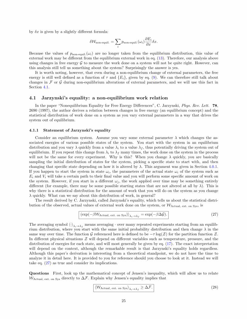
by δx is given by a slightly different formula:

δWnon-equil. =∑i

pnon-equil.(ωi)∂Ei∂x

δx.

Because the values of pnon-equil.(ωi) are no longer taken from the equilibrium distribution, this value ofexternal work may be different from the equilibrium external work in eq. (13). Therefore, our analysis aboveusing changes in free energy G to measure the work done on a system will not be quite right. However, canthis analysis still tell us something about the system? Surprisingly the answer is yes.

It is worth noting, however, that even during a non-equilibrium change of external parameters, the freeenergy is still well defined as a function of τ and Ei, given by eq. (9). We can therefore still talk aboutchanges in F or G during non-equilibrium alterations of external parameters, and we will use this fact inSection 4.1.

4.1 Jarzynski’s equality: a non-equilibrium work relation

In the paper “Nonequilibrium Equality for Free Energy Differences”, C. Jarzynski, Phys. Rev. Lett. 78,2690 (1997), the author derives a relation between changes in free energy (an equilibrium concept) and thestatistical distribution of work done on a system as you vary external parameters in a way that drives thesystem out of equilibrium.

4.1.1 Statement of Jarzynski’s equality

Consider an equilibrium system. Assume you vary some external parameter λ which changes the as-sociated energies of various possible states of the system. You start with the system in an equilibriumdistribution and you vary λ quickly from a value λi to a value λf , thus potentially driving the system out ofequilibrium. If you repeat this change from λi to λf many times, the work done on the system in the processwill not be the same for every experiment. Why is this? When you change λ quickly, you are basicallysampling the initial distribution of states for the system, picking a specific state to start with, and thenchanging that specific state depending on how it is altered by λ. This argument was given in Section 4.0.1.If you happen to start the system in state ωi, the parameters of the actual state ωi of the system such asEi and Vi will take a certain path to their final value and you will perform some specific amount of work onthe system. However, if you start in a different ωj , the work applied over time may be something entirelydifferent (for example, there may be some possible starting states that are not altered at all by λ). This iswhy there is a statistical distribution for the amount of work that you will do on the system as you changeλ quickly. What can we say about this distribution of work, in general?

The result derived by C. Jarzynski, called Jarzynski’s equality, which tells us about the statistical distri-bution of the observed, actual values of external work done on the system, or WActual, ext. on Sys, is

〈exp(−βWActual, ext. on Sys)〉λi→λf= exp(−β∆G). (27)

The averaging symbol 〈·〉λi→λfmeans averaging · over many repeated experiments starting from an equilib-

rium distribution, where you start with the same initial probability distribution and then change λ in thesame way over time. The function G referenced here is defined to be −τ log(Z) for the partition function Z.In different physical situations Z will depend on different variables such as temperature, pressure, and thedistribution of energies for each state, and will most generally be given by eq. (17). The exact interpretationwill depend on the context, although the remarkable result is that Jarzynski’s equality holds regardless.Although this paper’s derivation is interesting from a theoretical standpoint, we do not have the time toanalyze it in detail here. It is provided to you for reference should you choose to look at it. Instead we willtake eq. (27) as true and consider its implications.

Questions First, look up the mathematical concept of Jensen’s inequality, which will allow us to relateWActual, ext. on Sys directly to ∆F . Explain why Jensen’s equality implies that

〈WActual, ext. on Sys〉λi→λf≥ ∆F . (28)

25

Next, remember that F measures the work that you can extract back out of the system through a reversibleprocess, and so we can say that ∆F = WReversible, ext. on Sys, or the reversible external work done on asystem. Thus we can define something called dissipated work,

WDis =WActual, ext. on Sys −WReversible, ext. on Sys.

With this definition, eq. (28) implies that

〈WDis〉λi→λf≥ 0 and 〈exp(−βWDis)〉λi→λf

= 1 (29)

Try to explain why the result quoted above makes intuitive sense based on your real world experience, bothfor the case of positive external work and negative external work. Your explanation does not need to bemathematically rigorous; we just want to see how you interpret the above result in terms of the real world.

4.1.2 Experimental test of Jarzynski’s equality

Equation (28) roughly states that energy is dissipated on average during non-equilibrium changes. Notsurprisingly, this fact was known empirically for a long time before the more precise eq. (27) was statedby Jarzynski. Naturally, when eq. (27) was theoretically proposed, it became necessary to test its implica-tions experimentally to ensure that its predictions did not conflict with experiment. We will consider onepaper which explores Jarzynski’s equality experimentally: “Equilibrium Information from NonequilibriumMeasurements in an Experimental Test of Jarzynski’s Equality”, J. Liphardt et al., Science 296, 5574 (2002).

Questions Here you are asked to read the above paper by J. Liphardt et al. and answer a few keyquestions about its results. We suggest that you skim the paper once, focusing on general concepts and onunderstanding the data in the various figures, but moving on if a concept takes too much of your time tounderstand, or if it just seems downright unrelated to anything we’ve talked about in this document (wewon’t ask you questions about every detail of the paper). After this initial reading, you should try to answerspecific questions posed below by rereading specific sections of the paper in depth.

Please answer the following questions which roughly follow the chronological order of the paper. Thequestions generally do not focus on minute details that require an understanding of biology, and neithershould your answers. Focus on interpreting results in terms of concepts introduced in this document.

1. Describe in your own words the experimental setup. What are the physical parts involved?

2. What can you consider to be the reservoir for this system?

3. How do the experimenters measure work done on the system?

4. How do the experimenters measure the actual change in free energy, ∆G, between the initial and finalstates? (Note that this paper uses the Gibbs Free energy in Jarzynski’s equality, which is valid becausetheir physical system is coupled to a bath of constant temperature and pressure.) As you have probablyrealized, computing G = −τ log(Z) from the probability distribution would be nearly impossible in allbut the simplest situations. Hint: read through page 2 of the paper if you cannot figure this out andlook for the symbol ∆G.

5. How do the experimenters test Jarzynski’s equality? Remember that the experimenters have one objec-tive measure of ∆G using the method you found above. Jarzynski’s equality also provides an estimateof ∆G by averaging something (what is it?) over multiple experiments. What do the experimenters dowith these two, potentially different values for ∆G that they obtain?

6. What is different about the experiments in Fig. 2(a) that generate the red curves from the experimentsthat generate the blue curves? Explain why in Fig. 2(a) the two blue curves lie almost on top of eachother everywhere while the two red curves do not.

7. Consider Fig. 3(a). What is being plotted? You should refer to the caption. Why does the estimate of∆G from Jarzynski’s equality underestimate the actual value of ∆G? You may find it helpful to rereadthe bottom two paragraphs of the left column of the page containing Fig. 3.

26

8. Consider Fig. 3(b). What is the main difference between this data and the data from Fig. 3(a)? Focuson the dashed lines and solid lines. What does it mean that the solid lines are higher than 0 on thegraph? What does it mean that the dashed lines are approximately 0 for any extension length? Thisresult is, more or less, the most important result of the paper.

9. Consider Fig. 3(c), Fig. 3(d), and Fig. 3(e). What is plotted is the probability of obtaining certainvalues of dissipated work, or actual work observed on the system minus the change in free energy. Fig.3(c) shows the probability distribution after you have extended from 0 nm to 5 nm, while (d) showsthe probability distribution after extension from 0 nm to 15 nm, and (e) after extension from 0 nm to25 nm. The blue, green, and red data sets represent probability distributions for different switchingrates (speeds at which the system is altered). Blue corresponds to the blue lines in Fig. 3(a), and redand green correspond to the red and green data in Fig. 3(b).

Is the switching rate for the blue data set faster or slower than the switching rate for the red data set?Can you explain why it makes sense that the average dissipated work in the blue data set is centeredaround 0?

Focus on the red data set in Fig. 3(e). This is a probability distribution with a relatively large spreadand an average that is positive. From Jarzynski’s equality, we showed that eq. (29), or

〈exp(−βWDis)〉λi→λf= 1

should hold true. Why is it that a distribution like the red distribution with a positive average butlarge spread can still satisfy this equation? To answer this, you might want to consider which datapoints are weighted more in computing this average than others. You do not have to be mathematicallyrigorous.

After answering these questions, you hopefully understand what experiment was performed in this paper andhow the data can be interpreted to be a valid test of Jarzynski’s equality. The end result of this paper is thatJarzynski’s equality is confirmed within experimental error. We can therefore accurately predict changes inthe equilibrium free energy of a system (which is also the work we can possibly reliably extract from thesystem) by performing multiple, fast, non-equilibrium experiments and averaging these results according toJarzynski’s equality.

Thus, in a broader sense, we have learned that highly abstract mathematical frameworks can actuallybe useful for predicting concrete results in physical systems in the world around us. Moreover, these resultshold for systems under very few idealizing assumptions. Indeed, the system does not need to be infinitelysmall, the bath does not need to be infinitely large, and we don’t have to change the parameters of thesystem infinitely slowly.

4.2 Dissipation in computational systems

Perhaps surprisingly, the theoretical results derived earlier in this paper also allow us to explore thethermodynamic limits of computation. In effect, we want to analyze how much energy we dissipate as weperform a computation on a computer, if any. In order to analyze this situation, we must first define atheoretical model of a computing system, meaning define what its logical components are, and we mustspecify how the computer fits into the framework of a system and reservoir that is used throughout thispaper. We can then consider how its free energy changes as a computation is performed, and consider howmuch energy is dissipated.

4.2.1 Reversible or irreversible computation?

As has been discussed above, when a system’s state changes reversibly, the least amount of energy isdissipated (on average) that is possible. However, you often want a system to compute something quickly, inwhich case you want to drive the system to change quickly, and this can push the system out of equilibrium,leading to more dissipated energy on average.

While the question “how much energy am I willing to dissipate just to have a faster computation?” isan important question, we will not concern ourselves with it here. Rather, we will try to determine limits

27

on the energy dissipated during a computation which is performed slowly enough so that the system alwaysremains close to the equilibrium probability distribution.

4.2.2 The AND gate as a logical operation

Rather than analyze an entire computer as a system all at once, we will analyze its smallest components.One of the simplest digital computing functions is to take two bits, which are units of information that canbe either 0 (false) or 1 (true), and perform the AND operation. This operation outputs 1 only if both inputsare 1, and outputs 0 otherwise. Thus, (0, 1)→ (0), (1, 0)→ (0), (0, 0)→ (0), and (1, 1)→ (1).

It turns out that most modern computers can be built entirely from AND gates and a few other funda-mental building blocks, such as OR gates and NOT gates (which do exactly what they sound like they mightdo. Feel free to look them up). However, because the AND gate is widely used, we will focus on the ANDgate in the discussion below, and leave it to the reader’s imagination to generalize these concepts further.

4.2.3 A physical model

We can imagine an AND gate as a little machine that takes two logical inputs and produces one logicaloutput. There are many different ways to implement this machine in the physical world, just as there aremany ways to represent 1 and 0, and so it becomes difficult to say something generally meaningful aboutthe energy costs of an AND gate. However, we can say something meaningful if we translate the concept ofthe AND gate into the language of a system coupled to a reservoir with a statistical distribution of energies.

Our conceptual model is this: imagine a system with two “ports”, port A and port B. These ports caneach take on the value 0 or 1. To compute the logical operation of an AND gate on two bits, you load theinput bits into port A and port B. Next, the computation is applied to the two bits, and then the answer isdisplayed on port A, leaving the other port B to randomly be either 0 or 1.

How do we compare this to a system and reservoir model? We consider the two bits to be the systemwhich is coupled to an energy reservoir, a computer agent, and a human agent. This system has 4 possiblestates, corresponding to (0, 0), (1, 1), (1, 0), and (0, 1). There are two external actors which interact withthe system: the human agent that sets the initial values of the gates, and the computational agent whichchanges the initial state of the system to the final state of the system according to the logical rules of theAND gate. The initializer agent sets the initial values, steps back, and lets the computer interact with thesystem to put it into its final state, which can then be observed. While there may be other ways of conceivingof a computer, the physical results below are best understood with this model.

4.2.4 Operation of the AND gate from the perspective of statistical mechanics

This section goes through the sequence of steps that a computation consists of, and determines the valueof various statistical mechanical quantities during each step. Ultimately, this allows us to derive the amountof energy dissipated when performing a single computation.

Questions Assume that the system has exactly 4 possible states for port A and B: (0,0), (0,1), (1,0), and(1,1). We will call these states ω1, ω2, ω3, and ω4 respectively. We imagine that all of these states have someenergy Ei, and that the states are populated as usual in an equilibrium probability distribution, accordingto the factor exp(−βEi)/Z. Imagine that all of these states start out with the same energy Ei = ε. Thisresults in an initial value of the free energy which we will call FBefore init. = 〈E〉− τσSys. What is this value?

Next, as the external agent who initializes the ports, we choose to load a certain starting state into thecomputer. For example, to load ω2 = (0, 1), we raise all Ei with i 6= 2 to Ei ∼ ∞. If we do this, what isthe resulting value of 〈E〉? Hint: the limit as x → ∞ of xe−x is 0. What is the resulting value of σSys?Therefore, what is the resulting value of F? Call this value FBefore comp.. How much work did we have todo to cause this change? To be clear, we as the external agent that initializes the ports are doing this work.

At this point, we step back from the system and we let the computer perform a computation on thesystem. This operation is a deterministic map from initial to final configurations of the system according tothe logical operation of an AND gate. For example, because we are considering an AND gate, if we werein ω2 = (0, 1) initially, the final state has port A = 0 and port B undetermined. Therefore, the final stateis either ω1 = (0, 0) or ω2(0, 1), with equal probability. The computer is considered as an external agent

28

distinct from the system, so from the perspective of the system, the computer does work on the system andchanges Ei in some way, just as was done by the human agent during the initialization process. In thisinterpretation, the computer must have brought E1 down from E1 ∼ ∞ to E1 = ε, so that ω1 and ω2 wereequally likely, while ω0 and ω3 are impossible. When changing this energy, the computer did work on thesystem. Was this positive or negative work? You can find out by computing the change in free energy. Callthe new free energy after this change FAfter comp..

Once we have computed these various free energy changes, we need only keep track of where work is doneand where energy is dissipated during the process of computation. The next section will discuss this processin more detail.

4.2.5 Where is energy dissipated?

During the procedure of computation, we do work on the system to start it in one of the computationalbasis states. We step back, and then the computer steps in and exchanges energy with the system. The systemis then in its final state. The work we do to initialize the system is FBefore comp. − FBefore init. = τ log(4) =2τ log(2). The work that the computer does when it exchanges energy with the system is FAfter comp. −FBefore comp. = −τ log(2). Note that this work done by the computer on the system is negative so that thecomputer extracts energy from the system. Lastly, if we wanted to reinitialize the system into a differentωi after finishing a computation, it is not hard to show that we would have to do an additional amount ofwork given by FBefore comp.−FAfter comp. = τ log(2). From this we see that, in the course of one computationwhere the system goes from FAfter comp. to FBefore comp. to FAfter comp., we put in τ log(2) worth of energyto the system, and then the computer takes out τ log(2) worth of energy. It is not clear exactly where thisenergy goes after the computer extracts it, but the point is that we as the initializers no longer controlthe energy, and we no longer can get it back out of the system directly.11 This loss of energy means thatcomputations with an AND gate costs us as the human initializer τ log(2) worth of energy on average percomputational cycle.

Questions It is common to look at the above energy cost of computation and call it “irreversible com-putation” because of the energy cost associated. Why is this potentially a misnomer? Is the energy reallydissipated, or is it just stored in a different system (like the computer)? Remember that we are still assumingthat we are operating slowly enough so that the system remains in equilibrium with the reservoir at all times.

It is important to realize that the computer itself is a system coupled to a reservoir. In real physicalcomputers, the energy τ log(2) is extracted during a computation and resides in the core of the computer.The physical assumption is then that the energy extracted into the computer is eventually dissipated as heatloss, and is therefore well and truly irrecoverable.

4.2.6 Generalizing the computational model

It may have occurred to you that having only 4 states (not 4 logic states but 4 states total) available forthe system isn’t realistic.

Question Consider if, instead of 4 states, there were 40 states of the system possible, all with the sameinitial energy. Further assume that 10 of these states correspond to each of the 4 combinations of port Aand port B. In this case, we can still perform computation by changing the energy of each set of 10 statesat once. Argue why this does not change the essential conclusion that the energy cost of one sequence ofcomputation is τ log(2). You will have to consider the same set of steps that we used above to originallyderive the τ log(2) loss of energy per computation.

Additional information for your own interest This analysis can be extended further using the conceptof relative entropy to show that δσSys = δσLogic gates (meaning that the entropy of the whole system changes

11Perhaps there is a conceivable way of getting the energy back out of the computer, but we will not consider that here.

29

with the entropy of the logical output of the system) as long as a few small constraints on the system’senergies are made.12

4.2.7 Computing without the cost

In the case described above, although we described the process of computation through changing theenergies of the various states, Ei, note that the average energy of the system, 〈E〉, never changed. Therefore,the change in free energy is −τσSys which is quite literally the energy available to be extracted from thesystem. Once again, the entropy of the system seems to be physically relevant.

This observation suggest that, if we can design a computer that does not change the entropy of thesystem as it changes the input state of the system to the output state, we can perform computations withoutthe associated energy cost. If the free energy does not change, then the average work we, or the computer,performed on the system was 0.

Questions Consider the case where the mapping of the computer between initial and final logic gates is 1to 1. That is, consider a logical operation that is not the AND gate. This means that for every input logicstate there is exactly one possible output logic state, and the reverse. Two examples of such gates for twobit operations are the NOT gate and the identity gate. You can also look up a gate called to Toffoli gate foranother example, although this gate uses more computational bits.

If the computer is programmed to carry out this type of gate operation, what will be the change in theentropy of the system from before the computation to after the computation? Assume that we keep averageenergy fixed still, just as before. Does repeatedly performing this operation cost any energy on the part ofthe observer? Does the computer extract any energy as it performs its computation? Explain why. Thesetypes of logic gates are often referred to as “reversible” gates because the computation itself, if performedin near equilibrium, does not extract any energy on average from the system.

Perform a little research into modern computational systems to answer the question “how close to thethermodynamic limits of computation are modern computers?” In particular, try to find information aboutmodern physical implementations of the AND gate, and determine the energy dissipated in one logicaloperation. Is it close to τ log(2) or is it much larger? You may have to assume a certain temperature ofthe system and use the fact that τ = kBT , where kB is Boltzman’s constant and T is the temperature inKelvin (really temperature should be measured in units of energy, but historical reasons ensure that it isnot). With these results, can you argue whether classical computing systems are limited by the theoreticalthermodynamic limits of computation, or rather by inherent inefficiencies in the physical implementationsof computing architectures.

12One possible set of constraints is derived by decomposing the entropy of the states into the entropy of the logical outputports plus the relative entropy of the states given the value of the output ports. The assumptions that must then be madeare assumptions to ensure that the the relative entropy term is constant, so that changes in the full entropy of the system areprecisely changes in the entropy of the logical output ports.

30