2021 SISG Module 8: Bayesian Statistics forGenetics

Lecture 5: Multinomial and Poisson Models

Jon Wakefield

Departments of Statistics and BiostatisticsUniversity of Washington

1 / 67

Outline

Introduction and Motivating ExamplesInference for Parameters of Interest

Bayesian Analysis of Multinomial DataDerivation of the Posterior and Prior Specfication

Bayes Factors

Poisson Modeling of Count Data

AppendixBayes Factor DetailsNon-Conjugate Analysis

2 / 67

Introduction

3 / 67

Introduction

I In this lecture we will consider the Bayesian modeling of countdata, in particular multinomial and Poisson data, with anextension to negative binomial.

I The examination of Hardy-Weinberg equilibrium will be used tomotivate a multinomial model.

I Again, conjugate priors will be used.

I Sampling from the posterior will be emphasized as a method forflexible inference.

I Bayes factors will be used as a measure of evidence forhypothesis testing.

I We will fit simple Poisson and negative binomial models to anAIDS example dataset.

4 / 67

Motivating Example: Testing for HWE

I For simplicity we consider a diallelic marker, and suppose weobtain a random sample of genotypes for n individuals.

I The form of the data isGenotype Total

A1A1 A1A2 A2A2

Count n1 n2 n3 nPopulation Frequency q1 q2 q3 1

I So the model contains 3 probabilities (which sum to 1) q1,q2,q3;hence, there are 2 free parameters.

I Suppose the proportions of alleles A1 and A2 in a givengeneration are p1 and p2 = 1− p1.

I In terms of q1,q2,q3:

p1 = q1 +q2

2

p2 =q2

2+ q3

5 / 67

Motivating Example: Testing for HWE

I HWE is the statistical independence of an individual’s alleles at alocus.

I Under HWE, the probability distribution for the genotype of anindividual in the next generation is:

GenotypeA1A1 A1A2 A2A2

Proportion p21 2p1p2 p2

2 1

I Reasons for deviation from HWE include: small population size,selection, inbreeding and population structure.

6 / 67

A Real Example

Lidicker et al. (1997) examined genetic variation in sea otterpopulations (Enhydra lutris) in the eastern Pacific.

I Locus EST gave the data n1 = 37,n2 = 20,n3 = 7, with n = 64.

I Are these frequencies consistent with HWE?

I The MLEs are:

q̂1 =3764

= 0.58 q̂2 =2064

= 0.31 q̂3 =7

64= 0.11

p̂1 =37× 2 + 20

128= 0.73 p̂2 =

20 + 7× 2128

= 0.27.

I For these data the exact p-value for

H0 : q1 = p21, q2 = 2p1p2, q3 = p2

2

is 0.11.7 / 67

A Toy Example

In this made up example we have n = 100 so calculations are simpler.

Example:I Consider the data n1 = 88,n2 = 10,n3 = 2.

I Are these frequencies consistent with HWE?

I The MLEs are:

q̂1 = 0.88 q̂2 = 0.10 q̂3 = 0.02p̂1 = 0.93 p̂2 = 0.07

I For these data the exact p-value for

H0 : q1 = p21, q2 = 2p1p2, q3 = p2

2

is 0.0654.

8 / 67

Critique of Non-Bayesian Approach

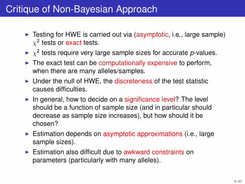
I Testing for HWE is carried out via (asymptotic, i.e., large sample)χ2 tests or exact tests.

I χ2 tests require very large sample sizes for accurate p-values.I The exact test can be computationally expensive to perform,

when there are many alleles/samples.I Under the null of HWE, the discreteness of the test statistic

causes difficulties.I In general, how to decide on a significance level? The level

should be a function of sample size (and in particular shoulddecrease as sample size increases), but how should it bechosen?

I Estimation depends on asymptotic approximations (i.e., largesample sizes).

I Estimation also difficult due to awkward constraints onparameters (particularly with many alleles).

9 / 67

Parameters of Interest

Genotype TotalA1A1 A1A2 A2A2

Population Frequency q1 q2 q3 1

I Rather than q1,q2,q3, we may be interested in other parametersof interest.

I In the HWE context: Let X1 and X2 be 0/1 indicators of the A1allele for the two possibilities at a locus; so X1 = X2 = 1corresponds to the genotype A1A1.

I The covariance between X1 and X2 is the disequilibriumcoefficient:

D = q1 − p21

Under HWE q1 = p21, and the covariance is zero.

I Another quantity of interest (Shoemaker et al., 1998) is

ψ =q2

2q1q3

.

Under HWE, ψ = 4.10 / 67

Parameters of Interest

I The inbreeding coefficient is

f =q1 − p2

1p1p2

I The variance of X1 and X2 is p1(1− p1) = p1p2 and so f is thecorrelation.

I We may express q1,q2,q3 as

q1 = p21 + p1(1− p1)f

q2 = 2p1(1− p1)(1− f )

q3 = (1− p1)2 + p1(1− p1)f

I Positive values of f indicate an excess of homozygotes (and mayindicate inbreeding), while negative values indicate an excess ofheterozygotes.

11 / 67

Bayesian Analysis of Multinomial Data

12 / 67

Bayes Theorem

Genotype TotalA1A1 A1A2 A2A2

Count n1 n2 n3 nPopulation Frequency q1 q2 q3 1

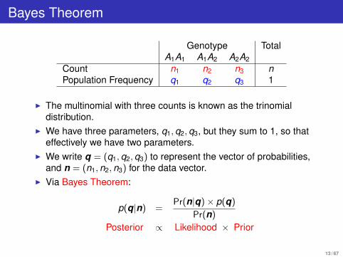
I The multinomial with three counts is known as the trinomialdistribution.

I We have three parameters, q1,q2,q3, but they sum to 1, so thateffectively we have two parameters.

I We write q = (q1,q2,q3) to represent the vector of probabilities,and n = (n1,n2,n3) for the data vector.

I Via Bayes Theorem:

p(q|n) =Pr(n|q)× p(q)

Pr(n)

Posterior ∝ Likelihood × Prior

13 / 67

Elements of Bayes Theorem: The Likelihood

I We assume n independent draws with common probabilitiesq = (q1,q2,q3).

I In this case, the distribution of n1,n2,n3 is multinomial:

Pr(n1,n2,n3|q1,q2,q3) =n!

n1!n2!n3!qn1

1 qn22 qn3

3 . (1)

I For fixed n, we may view (1) as a function of q – this is thelikelihood function.

I The maximum likelihood estimate (MLE) is

q̂ =(n1

n,

n2

n,

n3

n

).

I The MLE gives the highest probability to the observed data,i.e. maximizes the likelihood function.

14 / 67

The Dirichlet Distribution as a Prior Choice for aMultinomial q

I Once the likelihood is specified we need to think about the priordistribution.

I We require a prior distribution over (q1,q2,q3) — notstraightforward since the three probabilities all lie in [0,1], andmust sum to 1.

I A distribution that satisfies these requirements is the Dirichletdistribution, denoted Dirichlet(v1, v2, v3) and has density:

p(q1,q2,q3) =Γ(v1 + v2 + v3)

Γ(v1)Γ(v2)Γ(v3)× qv1−1

1 qv2−12 qv3−1

3

∝ qv1−11 qv2−1

2 qv3−13

where Γ(·) denotes the gamma function.

15 / 67

The Dirichlet Distribution as a Prior Choice for aMultinomial q

I The Dirichlet(v1, v2, v3) prior:

p(q1,q2,q3) =Γ(v1 + v2 + v3)

Γ(v1)Γ(v2)Γ(v3)× qv1−1

1 qv2−12 qv3−1

3

∝ qv1−11 qv2−1

2 qv3−13 .

I v1, v2, v3 > 0 are specified to reflect prior beliefs about(q1,q2,q3).

I The dirichlet distribution can be used with general multinomialdistributions (i.e. for k = 2,3, ... categories).

I The beta distribution is a special case of the dirichlet when thereare two categories only.

16 / 67

Dirichlet Prior

I The mean and variance are

E[qi ] =vi

v1 + v2 + v3=

vi

v

var(qi ) =E[qi ](1− E[qi ])

v1 + v2 + v3 + 1=

E[qi ](1− E[qi ])

v + 1

for i = 1,2,3, where v = v1 + v2 + v3.I Large values of v increase the influence of the prior.I The dirichlet has a single parameter only (v ) to control the

spread for all of the dimensions, which is a deficiency.I The quartiles may be empirically calculated from samples.

17 / 67

q1

Frequenc

y

0.0 0.2 0.4 0.6 0.8 1.0

0200

400600

800

q2

Frequenc

y

0.0 0.2 0.4 0.6 0.8 1.0

0200

400600

8001000

q3

Frequenc

y

0.0 0.2 0.4 0.6 0.8 1.0

0200

400600

8001000

0.0 0.2 0.4 0.6 0.8 1.0

0.00.2

0.40.6

0.81.0

q1

q 2

0.0 0.2 0.4 0.6 0.8 1.0

0.00.2

0.40.6

0.81.0

q1

q 3

0.0 0.2 0.4 0.6 0.8 1.0

0.00.2

0.40.6

0.81.0

q2

q 3

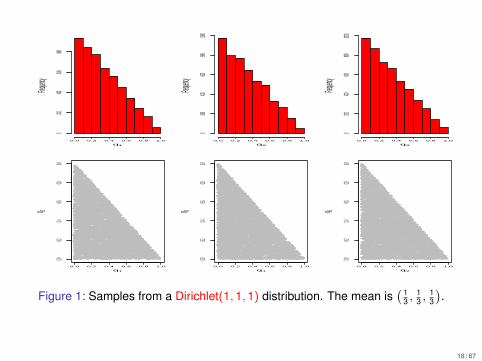
Figure 1: Samples from a Dirichlet(1, 1, 1) distribution. The mean is( 1

3 ,13 ,

13

).

18 / 67

0.00

0.25

0.50

0.75

1.00

0.00 0.25 0.50 0.75 1.00q1

q 2

20

40

60count

Figure 2: q1, q2 samples from a Dirichlet(5, 5, 5). The mean is( 1

3 ,13

).

19 / 67

q1

Freq

uenc

y

0.0 0.2 0.4 0.6 0.8 1.0

050

100

150

q2

Freq

uenc

y

0.0 0.2 0.4 0.6 0.8 1.0

050

100

150

q3

Freq

uenc

y

0.0 0.2 0.4 0.6 0.8 1.0

050

100

150

●

●

●

●

●

●

●

●

●

●●

●

●

●

●

●

●

●●

●

●

●

●

●

●

●

●

●

●

●

●

●

●●

●●

●

●●

●

●

●

●

●

●

●

●

●

●

●

●

●

●

●

●

●

●

●

●

●

●

●

●●

●

●

●

●

●

●●

●

●

●

●

●

●

●●

●

●

●

●

●

●

●

●

●

●

●●

●

●

●

● ●●

●

●

●

●

●

●

●

●

●

●

●

●

●

●

●●

●

●

●

●

●

●● ●

●

●

●●

●●

●

●

●

●

●

●

●

●●●

●

●

●

●

●

●●

●

●

● ●

●

●●●

●

●

●

●

●

●

●

●

●

●

●

●

●

●

●

●

●

●

●

●

●

●

●

●

●

●

●

●

●

●

●

●

●

●

●

●

●

●

●●

●

●● ●●

●●

●

●

●

●

●

●

●●

●

●

●

●

●

●

●

●

●

●

●

●

●

●

●

●

●

● ●

●

●

●●

●

●

● ●●

●

●

●

●

●●●

●●

●

●

●

●

●

●

●

●

●

●

●

●●●

●● ●●

●

●

●

●

●

●

●

● ●

●

●

●

●

●

●

●●

●

●

●●

●

●

●

●

●

●

●

●

●●

● ●

●

●

●

●

●

●●

●

●

●

●

●

●

●

●

●

●

●

●

●●

●

●

●

●

●

●

●

● ●

●

●

●

●

●

●

●

●●

●

●

●

●●

●

●

●

●

●

●●

●●

●

●

●●●●

●

● ●

●

●

●

●

●

●

●

●

●●

●

●●

● ●

●●

●●

●

●

●

●

●●

●

●

●●

●

●

●

●

●● ●

●

●

●

●

●

●

●

●

●

●

●

●

●

●

●

●

●●

●

●

●●●

●

●

●

●

● ●

●

●

●

●

●

●

●

●

●

●

●

●

●

●

●

●

● ●●●

●

●

●

●

●●

●

●

●

●

●

●

●●

●

●

●

●

●

●

● ●●

●

●●

●

●

●

●

●

●

●

●

●

●

●

●

●

●●

●●

●

●

●●

●●●

●

●

●

●●

●

●

●

●

●

●●

●●●

●●

●

● ●

●

●

●

●

●

●

●

●

●

●

●

●

●

●

●●

●

●

●

●

●

●

●

●

●

●

●

●●

●

●

●

●

●

●

●●

●

●

●

●

●

●

●

●

●●●

●

●

●

●

●

●

●

●

●

●

●

●

●●

●

●

●

●

●

●

●

●

●

●

●

●

●

●

●

●●

●

●●

●

●

●●

●●

●

●●

●

●●

●

●

●●

●

●●

●

●

●

●

●

●

●

●

●●

●

●

●

●

●

●

●

●●

●

●

●

●

●

●●

●

●

●

●

●

●

●

● ●

●

●

●

●

●●

●

●

●

●

●

●

●

● ●

●

●

●

●

●

●

●

●

●

●

●●

●●

●

●

●

●

●●

●

●

●

●

●

●

●

●

●

●

●

●

●●

●

●

●

●

●

●

●● ●

●●

●●●

●

●

●

●

●

●

●

●

●

●

●● ●

●

●

●

●

●● ●●

●

●

● ●

●

●

●

●

●

●●

●●

●

●

●

●

●

● ●

●

●

●

●●●

●

●●

●

●

●

●

●●

●●

●

●

●

●

●●

● ●

●

●●

●

●●

●●

●

●

●

●

●

●

●●

●

●●

●

●

●

●●

●

●

●

●

●

●

●●

●

●

●

●

●

● ●

●

●

●

●

●

●

●

●

●

●

● ●

●

●

● ●

●

●

●

●●

●

●

●

●●

●●

●

●

●

●

●●

●

●

●

●

●

●

●

● ●

●●

●

●

●

●

●

● ●

●

●

●●

●

●

●

●

● ●

●

●

●

●

●

●

●

●

●

●

●

●

●

●

●

●

●

●●

●●

●

●●

●

●

●

●

●●

●

●

● ●

●

●

●

●●●

●●

●

●

●

●●

●●

●

●

●

●

● ●

●

●● ●

●

●

●

●

●

●

●

●

●

●●

●

●

●

●

●

●

●

●

●

●

●

●

●●●

●

●

●●

●

●●

●

●

●

●

●

●

●

●

● ●

●

●

●

●

●

●

●●

●

●●

●

●●

●●

●●

●

●

0.0 0.2 0.4 0.6 0.8 1.0

0.00.2

0.40.6

0.81.0

q1

q 2

●

●

●

●

●

●

●

●●

●

●●

●

●

●

●

●

●

●

●

●

●

●

●

●

●

●

●

●

●

●

●

●

●

●

●

●

●

●

●

●

●

●

●

●

●

●

●

●

● ●

●

●

●

●

●

●

●

● ● ●

●

●

●●●

●

●●

●

●

●

●●●

●●

●

●

●

●

●●

●●

●●

●

●

●

●

●

● ●

●

●

●

●

●●

●

●

●

●●

●

●

●

●

●

● ●

●●●

●

●

●

●

●

●

●

●

●●

●●

● ●●

●

●

●

●

●●

●

●

●

●

●

●●●

●●

●

●

●

●

●

● ●●

●

●

●

●

●

●

●●

●

●

●●

●●

●

●

●

●

●

●

●

●

●

●●

●

●

●●

●

●●

●

●

●

●

●

●●

●

●

●

●

●

●

●

●

●●

●

●

●

●

●

●●

●

●

●

●

●

●

● ●●

●●

●

●

●

●

●

●

●

●

●

●

●

●

●

●

●●

●

●

●

●

●●

●

●

●

● ●

●

●

● ●

● ●

●

●●

●

●●

●

●

●

●●

●

●

●

●

●

●

●●

●●

●

●

●

●

●

●

●

●●

●

●

●

●

●

●●●●

●

●

●

●● ●

● ●●

●●●

●

●

●

●

●

●

●

●

●

●

●

● ●

●

●

●

●

●●

●

●

●

● ●

●

● ●

●

●

●

●●

●●

●

●

●

●

●

●

●

●

●●

●

●

●

●

●

●●

●●

●

●●

●

●

●●

●

●

●

●

●●

●●

●

●

●

●

●

●

●

●

●

●

●

●

●

●

●

●

● ●

●

●

●

●

●

●●

●

●

●

●

●

●

● ●●

●

●

●

●

●

●

●●●

●

●

●

●●

●

●

●

●

●

●

●

●

●

●

●

●

●

●

●

●

●

●

●

●

●

●

●●

●

●

●●

●●

●

●

●

●●●

●

●

●

●

●

●

●

●●

●

●

●

●●

●

●

●●

●

●

●

●

●

●

●

●

●

●

●●

●

●●

●

●

●

●

●

●●

●

●

●

●●

●

●

●

●

●

●

●

●

●

●●

●

●

●

●

●

●

●

●

● ●

●

●

●

●

●

●●

●

●

●

●

●

●●

●

●●

●

●

●

●

●

●

●

●●

●

●

●

●

●

●

●●

●●●

●

●

●

●●

●●

●

●

●

●

●

●

●

●

●

●

●

●

●

●

●

●

●

●

●

●

●

●●●

●●

●

●

●

●

●

●

● ●

●

●

●

●

●

●

●

●

●

●

●

●

●

●

●

●

●

●

●●

●

●●

●

●

●

●

●

●

●

●

●

●

●●

●●

●●

●

●

●

●

●

●

●

●

●

●

●

●

●

●

●

●

●

●●

●

●

●

●

●●●

●

●●●

●

●

●

●

●

●●

●

●

●

●

●●

●

●

●

●

●

●

●●

●●

●

● ●

●

●

●

● ●

●

●●

●

●

●

●

●

●

●

●

●

●

●

●

●

●

●

●

●

●

●

●

●

●●

●

●

●

●

●

●

●

●

●

●

●

●

●

●

●

●

●●

●

●●

●

●

●

●●

●

●

●●

●

●

●

●

●

●

●

●

●

●

●

●

●●●

●

●

●

●

●

●

●

●●

●

●

●●

●

●

●

●

●

● ●

●

●

●

●

●

●●

●

●

●

●

●

●

●

●

●

●●

●

●

●

●

●

●●

●

●●

●

●

●

●

●

●

●

●●

●

●

●●

●●

●

●

●●

●

●●

●

●

● ●

●

●

●

●

●

●

●●●

●

●

●

●

●

●

● ●

●

●

●

●

●

●●

●

●●

●●

●

●

●

●

●

●

●

●

●

●

●●

●●

●

●

●

●

●

●●● ●●

●

●

●●

●

●●

●

●

●

●

●

●

●

●

●

●

●●

●

● ●

●

●

●

●

●

●● ●

●

●●

●

●

●

●

●●

●

●

●

●●

●

●

●

●

●

●●

●

●

●

●

●●

●

●

●

●●

●

●

●

●

●

●

●

●●

●

●

●

●

●

●●●

●

● ●● ●

● ●●

●

●

●

●●●

●

●

●●

●

● ●

●

0.0 0.2 0.4 0.6 0.8 1.0

0.00.2

0.40.6

0.81.0

q1

q 3

●

●

●

●

●

●

●

●●

●

●●

●

●

●

●

●

●

●

●

●

●

●

●

●

●

●

●

●

●

●

●

●

●

●

●

●

●

●

●

●

●

●

●

●

●

●

●

●

●●

●

●

●

●

●

●

●

●●●

●

●

●● ●

●

●●

●

●

●

●● ●

● ●

●

●

●

●

●●

●●

● ●

●

●

●

●

●

●●

●

●

●

●

●●

●

●

●

●●

●

●

●

●

●

●●

●● ●

●

●

●

●

●

●

●

●

●●

●●

●●●

●

●

●

●

●●

●

●

●

●

●

●●

●●

●

●

●

●

●

●

●●●

●

●

●

●

●

●

● ●

●

●

●●

●●

●

●

●

●

●

●

●

●

●

● ●

●

●

● ●

●

●●

●

●

●

●

●

●●

●

●

●

●

●

●

●

●

● ●

●

●

●

●

●

●●

●

●

●

●

●

●

●● ●

●●

●

●

●

●

●

●

●

●

●

●

●

●

●

●

●●

●

●

●

●

●●

●

●

●

●●

●

●

●●

●●

●

●●

●

●●

●

●

●

●●

●

●

●

●

●

●

● ●

● ●

●

●

●

●

●

●

●

●●

●

●

●

●

●

●● ●●

●

●

●

●●●

●●●

● ●●

●

●

●

●

●

●

●

●

●

●

●

●●

●

●

●

●

● ●

●

●

●

●●

●

●●

●

●

●

● ●

●●

●

●

●

●

●

●

●

●

●●

●

●

●

●

●

●●

●●

●

●●

●

●

●●

●

●

●

●

●●

●●

●

●

●

●

●

●

●

●

●

●

●

●

●

●

●

●

●●

●

●

●

●

●

●●

●

●

●

●

●

●

●●●

●

●

●

●

●

●

●●●

●

●

●

●●

●

●

●

●

●

●

●

●

●

●

●

●

●

●

●

●

●

●

●

●

●

●

●●

●

●

●●

●●

●

●

●

●● ●

●

●

●

●

●

●

●

●●

●

●

●

●●

●

●

●●

●

●

●

●

●

●

●

●

●

●

● ●

●

● ●

●

●

●

●

●

●●

●

●

●

●●

●

●

●

●

●

●

●

●

●

●●

●

●

●

●

●

●

●

●

●●

●

●

●

●

●

●●

●

●

●

●

●

●●

●

● ●

●

●

●

●

●

●

●

●●

●

●

●

●

●

●

● ●

●●●

●

●

●

●●

● ●

●

●

●

●

●

●

●

●

●

●

●

●

●

●

●

●

●

●

●

●

●

●●●

●●

●

●

●

●

●

●

●●

●

●

●

●

●

●

●

●

●

●

●

●

●

●

●

●

●

●

●●

●

●●

●

●

●

●

●

●

●

●

●

●

●●

● ●

●●

●

●

●

●

●

●

●

●

●

●

●

●

●

●

●

●

●

●●

●

●

●

●

● ●●

●

●● ●

●

●

●

●

●

●●

●

●

●

●

●●

●

●

●

●

●

●

●●

●●

●

●●

●

●

●

●●

●

●●

●

●

●

●

●

●

●

●

●

●

●

●

●

●

●

●

●

●

●

●

●

●●

●

●

●

●

●

●

●

●

●

●

●

●

●

●

●

●

●●

●

●●

●

●

●

●●

●

●

●●

●

●

●

●

●

●

●

●

●

●

●

●

●●

●

●

●

●

●

●

●

●

●●

●

●

●●

●

●

●

●

●

●●

●

●

●

●

●

●●

●

●

●

●

●

●

●

●

●

●●

●

●

●

●

●

●●

●

● ●

●

●

●

●

●

●

●

● ●

●

●

● ●

● ●

●

●

●●

●

●●

●

●

●●

●

●

●

●

●

●

● ●●

●

●

●

●

●

●

●●

●

●

●

●

●

● ●

●

●●

●●

●

●

●

●

●

●

●

●

●

●

●●

● ●

●

●

●

●

●

● ●●●●

●

●

●●

●

●●

●

●

●

●

●

●

●

●

●

●

●●

●

●●

●

●

●

●

●

●●●

●

●●

●

●

●

●

● ●

●

●

●

●●

●

●

●

●

●

●●

●

●

●

●

●●

●

●

●

●●

●

●

●

●

●

●

●

●●

●

●

●

●

●

●● ●

●

●●●●

●● ●

●

●

●

●●●

●

●

●●

●

●●

●

0.0 0.2 0.4 0.6 0.8 1.0

0.00.2

0.40.6

0.81.0

q2

q 3Figure 3: Samples from a Dirichlet(6, 6, 6) distribution. The mean is

( 13 ,

13 ,

13

).

20 / 67

q1

Freq

uenc

y

0.0 0.2 0.4 0.6 0.8 1.0

050

100

150

200

250

q2

Freq

uenc

y

0.0 0.2 0.4 0.6 0.8 1.0

050

100

150

200

250

q3

Freq

uenc

y

0.0 0.2 0.4 0.6 0.8 1.0

010

020

030

040

0

●

●

●

●

●

●

●

●

●

● ●

●

●

●

●

●

●

●

●

●

●

●

●

●

●

●

●

●

●

●

●

●

●

●

●

●●

●

●

●

●

●

●

●

●

●

●

●

●

●

●

●

●

●

●

●

●

●

●

●

●

●

●

●

●●

●

●

●

●

●

●

●

●

●

●

●

●

●

●

●●

●

●

● ●

●

●

●

●

●

●

●

●

●

●

●

●

●

●

●

●

●

●●

●

●●

●

●

●

●

●

●

●

●

●

●

●

●

●

●

●

●

●

●

●

●

●

●

●

●

●

●

●●

●

●

●

●

●

●

●

●

●

●

●●

●

●

●

●●

●

●

●●

●

●

● ●

●

●

●●

●

●●

●

●

●

●●

●

●

●

●

●

●

●

●●

●

●

●

●

●

●

●

●

●

●

●

●

● ●

●

●●

●

●

●

●

●

●

●

●

●

●

●

●

●●

●

●

●

●

●●

●

● ●●

●

●

●

●

●

●

●

●

●●

●●

●

●

●

●

●●

●

●

●

●●

●

●

●

●

●

●

●

●

●

●

●

●

●

●

●

●

●

●

●

●

●

●

●●

●●

●●

●

●

●

●

●

●●

●

●

●

●

●●

●

●

●

●●●

●

●

●

●

●

●

●

●

●●

● ●

●

●

●

●

●

●

●

●

●

●

●

●

●

●

●

●

●

●

●

● ●

●

●

●

●

●

●

●

●●

●

●●

●

●

●

●

●

●

●

●

●●

●

●

●

●

●

●

●

●

●

●

●

●

●

●

● ●

●

●

●

●

●

●

●

●

●

●

●

●

●

●

●

●

●

●

●

●●

●

●

● ●

● ●

●

●

●

●

●

●

●

●

●

●

●

●

●

●

●

●

●●

●●

●

● ●

●

●

●

●● ●

●

●

●●

●

●

●

●

●

●

●

●●

●

●

●

●

●●●

●

●

●

● ●

●

●●

●

●

●

●

●

●

●

●

●

●

●●

●

●

●●●

●

●

●

●

●

●

●

●

●

●

●

●

●

●

●

●●

●

●

●

●

●

●

●

●

●

●

●

● ●

●●

●

●

●

●

●

●

●

●●

●●

●

●

●

●

●

●

●

●

●●

●

●

●

●

●

●

●

●

●

●

●

●

●

●

●●

●

●

●

●

●●

●●

●

●●

●

●

●

●

●

●

●

●

●

●

●

●

● ●●

●

●

●●

●

●

●

●

●

●

●

●

●

●

●●

●

●

●

●

●

●

●

●

●

●

●

●

●

●

●

●

●

●●

●

●

●

●

●

●

●

●

●

●

●

● ●

●

●

●

●

●

●

●●

●●

●

●

●

●

●

●

●

●

●

●●

●

●

●

●

●

●

●

●

●

●

●

●

●

●

●

●

●

●

● ●

●

●

●●

●●

●

●

●

●●

●

●

●

●

● ●

●

●

●

●

●

●

●

●

●

●

●

●

●

●

●●

●

●

●

●

●

● ●

●

●

●

●

●

●

●

●

●●

●●●

●

●

●

●

●

●

●

●

●

●

●

●

●

●●

●●

●●

●

●

●

●

●

●

●

●

●

●

●

●

●

●●●

●

●

●

●

●

●

●

●

●

●

●

●

●

●

●

●●

●

●

●

●

●

●

●

●

●

●

●

●

●

●

●

●

●

●

●

●

●

●

●

●

●

●

●

●

●

●

●

●

●

●

●●

●

●

●

●

●

●

●

●●

●

●

●●

●

●

●

●

●

●

●

●

●

●

●

●●●

●

●

●

●

●

●

●

●

●●

●

●

●

●

●

●

●

●

●●

●

●

●

●

●

●

●

●

●

●

●●

●

●

●

●

●

●

●

●

●●

● ●

●

●

●

●

●

●

●

●

●

●

●

●●

●

●

●●

●●

●

●

●

●

●

●

●

●

●

●●

●

●

●

●●

●

●

●

●

●●

●●

●●

●

●

●

●

●

●

●

●

●

●

●●

●

●

●●

● ●●

● ●

●● ●

●

●

●

●

●

●

●

●

●

●

●

●

●

●●

●

●

●●

●

●

●

●

●●

●

●●

●

●

●

●

●

●●

●

●

●

●

●●

●

●

●

●

●

●

●

●

●

●

●

●

●

●● ●●●

●

●

●

●

●

● ●

●

●

●●

0.0 0.2 0.4 0.6 0.8 1.0

0.00.2

0.40.6

0.81.0

q1

q 2

●

●

●

● ● ●

●

●

●

●

●

●

●

●●

●

● ●

●

●

●●

●

●

●●

●

●

●

●

●

●

●

●●

●

●

●

●● ●●

●

●

● ●●

●

●● ●

●

●

●

●●

●

●

●●

●

●

●

●

●

●●

●

●

●

●

●

●

●

●

●●●

●●

●

●

●

●

●

●

●

●

●

●

●

●

●

●

●

●

●

●

●

●

●

● ●●●

●

●●● ●

●

●

● ●

●●

●●

●

● ●

●

●

●

●

●

●

●● ● ●● ●●

●

●

●●

● ●●●

●

●

●

●●● ●●

●

●

●

●

●

●

●

●

●●

●●

●

●

●

● ●

● ●

●

●

●

●

●

●

●

●●

●

●

●

●●

●●

●

●

● ●●●

●●

●

●

● ●

●●

●● ●

●●

●●

●

●●

●

●

●●

● ●

●

●

●

●

●

●

●

●●●

●

●

●

●

●

●

●

● ●

●●●

●

●

●

●

●

●

●

●

●●

●

●●

●

●●

●

●●

●

●

●

●

●●●

●

●

●

● ●

●

●

●

●

●

●

●●●

●● ●

●●

●

●

●●

●

●

●

●●

●●

●

●●

●●

●

●

● ●

●●

●

●●

●

●●

●

●

●

● ●

●

●●

●

●

●

●

●

●

●

●

●

●

●

●●

●

● ●

●

●

●

●

●●

●● ●●

● ●

●●●

●●

●●

●

●● ●

●

●

●

●

●

●

●

●

●

●

●

●●

●

●●

●

●●●

●●●

●

●

●

●●

●●

●

●

●

●●●

●

●

●

●● ●●

●

●

●●

●

●

●

●●

●

●●

●

●● ●

●

●

●

●

●

●

●

●

●●

●

●

●

●

●●

●

●

●

●

●

●●●

●

●●

●

●●

●

●

●

●

●

●●

●●

●

●●

●

●

●

●

●●●

●

●

●

●

●

●

●

●● ●

●

●

●●

●

●

● ●●●

●

●

●

●

●●

●

●

●

●

●●

●

●● ●

●

●

●

●

●

●●●

●

●

●

●

●

●

●●●

●

●●● ●● ●● ●

●

●

●●

●●

●●

●● ●

●

●

●●

●

●●

●●

●

●●●

●

●

●

●

●

●

●

●

●

●

●

●

●

●

●

●

● ●

●

●

●

●●

●●

●

●

●●

●

●

●●

●

●●

●

●●● ●

●

●

●

●

●

●

●

●

●

●

●

●

●

●

●

●●

●● ●

●

●●

●

●

●● ●●

● ●

●

●

●

●●

●

●●

●

●

●●

●

●

●

●

●

●

●●

● ●

●

●

●

●

●

●●

● ●●

●

●

●

●

●

●

● ●

●

●

● ●

●

●

●●●

●

●●

●

●

●

●●

●●

●

● ●

●●

●

●●

●

●

● ●

●

●

●

●●

●●

●

●

●● ●

●●

●

●

●●●

●●

●

●●

●

●

●

●

●

● ●

●

● ●● ●●●

● ●

●

●●

●

●

●●

●

●

●

●

●

●

●

●

●●

●

●

● ●●

●

●

●●

●

●

●

●●

●

●

●●

●

●

●

●

●

● ●●

●

●●

●

●

●

● ●●

●

●

●

●●

●

● ●

● ●

●

●

●

●

●

●●

●

●

●

● ●

●

●

●

●

●

●●

●

●

●●

● ●

●

●●●

●

●

●

● ●●●

●

●

●

●●

●

●

●

●

●●●

●●

● ●

●

●

●

●

●

●

●

●●●

●

●

● ●●

● ●●

● ●●

●

●

●

●

●●

● ●

●

●

●● ●●

●

●

●●

●

●

●

●

●

●

●

●●

●●

●

●

●

●

●

●●

●●

●

●

●●

●●

●●

●

●●

● ●●●

●

●●

●

●

●●

●●

●

●●

●

●

●

●

●●

●

●

●

●

●●

●●

●

●

● ●● ●

●

●

●●●

● ●

●

● ●

●

●

●●

● ●

●

●

●

●

●●

●

●●●

●

●

●

● ●●

●

●

● ●●

●

●

●

●

●

●

●

●

●

0.0 0.2 0.4 0.6 0.8 1.0

0.00.2

0.40.6

0.81.0

q1

q 3

●

●

●

●●●

●

●

●

●

●

●

●

● ●

●

●●

●

●

● ●

●

●

●●

●

●

●

●

●

●

●

●●

●

●

●

● ●●●

●

●

●●●

●

●●●

●

●

●

● ●

●

●

●●

●

●

●

●

●

●●

●

●

●

●

●

●

●

●

● ●●

●●

●

●

●

●

●

●

●

●

●

●

●

●

●

●

●

●

●

●

●

●

●

●● ●●

●

●● ●●

●

●

●●

●●

●●

●

●●

●

●

●

●

●

●

● ●●● ●●●

●

●

●●

●●● ●

●

●

●

● ●●● ●

●

●

●

●

●

●

●

●

●●

● ●

●

●

●

●●

●●

●

●

●

●

●

●

●

●●

●

●

●

●●

●●

●

●

●● ●●

●●

●

●

●●

●●

● ●●

●●

● ●

●

●●

●

●

●●

●●

●

●

●

●

●

●

●

●● ●

●

●

●

●

●

●

●

●●

●● ●●

●

●

●

●

●

●

●

●●

●

● ●

●

●●

●

● ●

●

●

●

●

● ●●

●

●

●

●●

●

●

●

●

●

●

● ●●

● ●●

●●

●

●

●●

●

●

●

●●

●●

●

● ●

● ●

●

●

●●

●●

●

●●

●

●●

●

●

●

●●

●

●●

●

●

●

●

●

●

●

●

●

●

●

● ●

●

●●

●

●

●

●

●●

● ●●●

●●

●●●

●●

●●

●

●●●

●

●

●

●

●

●

●

●

●

●

●

●●

●

●●

●

●● ●

● ● ●

●

●

●

●●

●●

●

●

●

● ●●

●

●

●

●●● ●

●

●

● ●

●

●

●

●●

●

● ●

●

●●●

●

●

●

●

●

●

●

●

● ●

●

●

●

●

●●

●

●

●

●

●

●●●

●

●●

●

●●

●

●

●

●

●

●●

●●

●

●●

●

●

●

●

●●

●

●

●

●

●

●

●

●

●●●●

●

●●

●

●

●●●●

●

●

●

●

●●

●

●

●

●

●●

●

●●●

●

●

●

●

●

●● ●

●

●

●

●

●

●

●●●

●

●● ●●●● ●●

●

●

●●

●●

●●

● ●●

●

●

●●

●

●●

●●

●

● ●●

●

●

●

●

●

●

●

●

●

●

●

●

●

●

●

●

●●

●

●

●

●●

●●

●

●

●●

●

●

● ●

●

● ●

●

● ● ●●

●

●

●

●

●

●

●

●

●

●

●

●

●

●

●

●●

●●●

●

●●

●

●

●●● ●

●●

●

●

●

● ●

●

●●

●

●

● ●

●

●

●

●

●

●

●●

●●

●

●

●

●

●

●●

●●●

●

●

●

●

●

●

●●

●

●

●●

●

●

●● ●

●

●●

●

●

●

●●

●●

●

●●

●●

●

● ●

●

●

●●

●

●

●

●●

●●

●

●

● ●●

●●

●

●

● ●●

●●

●

●●

●

●

●

●

●

●●

●

●● ●●●●

●●

●

●●

●

●

●●

●

●

●

●

●

●

●

●

●●

●

●

●● ●

●

●

●●

●

●

●

●●

●

●

●●

●

●

●

●

●

●●●

●

●●

●

●

●

●● ●

●

●

●

● ●

●

●●

●●

●

●

●

●

●

●●

●

●

●

●●

●

●

●

●

●

●●

●

●

●●

●●

●

●● ●

●

●

●

●● ●●

●

●

●

●●

●

●

●

●

● ●●

●●

●●

●

●

●

●

●

●

●

●● ●

●

●

●●●

●●●

●●●

●

●

●

●

● ●

●●

●

●

● ●● ●

●

●

●●

●

●

●

●

●

●

●

●●

●●

●

●

●

●

●

●●

● ●

●

●

●●

●●

●●

●

●●

●●●●

●

●●

●

●

●●

●●

●

●●

●

●

●

●

●●

●

●

●

●

●●

● ●

●

●

●● ●●

●

●

●● ●

●●

●

●●

●

●

●●

●●

●

●

●

●

●●

●

●● ●

●

●

●

●●●

●

●

●●●

●

●

●

●

●

●

●

●

●

0.0 0.2 0.4 0.6 0.8 1.0

0.00.2

0.40.6

0.81.0

q2

q 3

Figure 4: Samples from a Dirichlet(6, 4, 1) distribution. The mean is( 611 ,

411 ,

111

)= (0.55, 0.36, 0.09).

21 / 67

0.00

0.25

0.50

0.75

1.00

0.00 0.25 0.50 0.75 1.00q1

q 2

25

50

75

count

Figure 5: Hexbin plot of q1, q2 samples from a Dirichlet(6, 4, 1) distribution.

22 / 67

0.2

0.4

0.6

0.8

0.25 0.50 0.75q1

q 2

5

10

15density

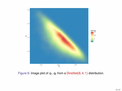
Figure 6: Image plot of q1, q2 from a Dirichlet(6, 4, 1) distribution.

23 / 67

Parameters of Interest

I Each of D, ψ and f are complex functions of q1,q2,q3 and givena Dirichlet prior for the latter do not have known posterior forms.

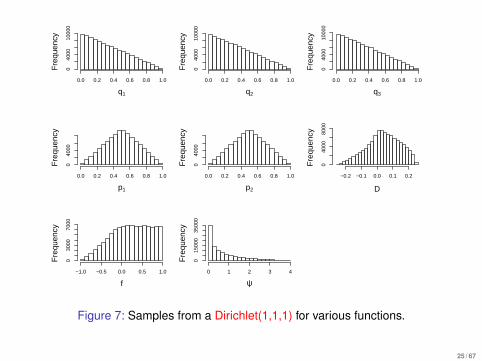
I The “flat” prior for q, Dirichlet(1,1,1), does not correspond to aflat prior for D, f , ψ, as Figure 7 shows.

I With a “flat” Dirichlet prior Dirichlet(1,1,1) the prior probabilitythat f > 0 is 0.67.

24 / 67

q1

Fre

quen

cy

0.0 0.2 0.4 0.6 0.8 1.0

040

0010

000

q2

Fre

quen

cy

0.0 0.2 0.4 0.6 0.8 1.0

040

0010

000

q3

Fre

quen

cy

0.0 0.2 0.4 0.6 0.8 1.0

040

0010

000

p1

Fre

quen

cy

0.0 0.2 0.4 0.6 0.8 1.0

040

00

p2F

requ

ency

0.0 0.2 0.4 0.6 0.8 1.0

040

00D

Fre

quen

cy

−0.2 −0.1 0.0 0.1 0.2

040

0080

00

f

Fre

quen

cy

−1.0 −0.5 0.0 0.5 1.0

030

0070

00

ψ

Fre

quen

cy

0 1 2 3 4

015

000

3500

0

Figure 7: Samples from a Dirichlet(1,1,1) for various functions.

25 / 67

−0.5

0.0

0.5

1.0

0.00 0.25 0.50 0.75q1

f

0.5

1.0

density

Figure 8: Image plot of q1, f from a Dirichlet(1, 1, 1) distribution.

26 / 67

−0.5

0.0

0.5

1.0

0.25 0.50 0.75q1

f

0.25

0.50

0.75

1.00

density

Figure 9: Image plot of p1, f from a Dirichlet(1, 1, 1) distribution.

27 / 67

Posterior Distribution

I Combining the Dirichlet prior, Dirichlet(v1, v2, v3), with themultinomial likelihood gives the posterior:

p(q1,q2,q3|n) ∝ Pr(n|q)× p(q)

∝ qn11 qn2

2 qn33 × qv1−1

1 qv2−12 qv3−1

3

= qn1+v1−11 qn2+v2−1

2 qn3+v3−13 .

I This distribution is another Dirichlet:

Dirichlet(n1 + v1,n2 + v2,n3 + v3).

I Notice: “as if” we had observed counts (n1 + v1,n2 + v2,n3 + v3).

28 / 67

Choosing a Prior

I The posterior mean for the expected proportion of counts in cell iis, for i = 1,2,3:

E[qi |n] =ni + vi

n + v

=ni

nn

n + v+

vi

vv

n + v= MLE×W + Prior Mean× (1−W)

where n = n1 + n2 + n3, v = v1 + v2 + v3.

I The weight W isW =

nn + v

which is the proportion of the total information (n + v ) that iscontributed by the data (n).

29 / 67

Choosing a Prior

I Recall the prior mean is (v1

v,

v2

v,

v3

v

)I These forms help to choose v1, v2, v3.I As with the beta distribution we may specify the prior means, and

the relative weight that the prior and data contribute: n and v areon a comparable scale.

I For example, suppose we believe that event 1 is four times aslikely as each of event 2 or event 3.

I Then we may specify the means in the ratios 4:1:1.I Suppose n = 24 and we wish to allow the prior contribution to be

a half of this total (and therefore a third of the completeinformation). Then the prior sample size is v = 12 and the priormean requirement gives

v1 = 8, v2 = 2, v3 = 2.

30 / 67

A Uniform Prior

0.0 0.2 0.4 0.6 0.8 1.0

0.0

0.2

0.4

0.6

0.8

1.0

q1

q 2

An obvious choice of parametersis v1 = v2 = v3 = 1 to give a priorthat is uniform over the simplex:

π(q1,q2,q3) = 2

for

0 < q1,q2,q3 < 1, q1+q2+q3 = 1

Note: not uniform over all parameter of interests, as we have seen.

31 / 67

Simple HWE Example

I The data isn1 = 88,n2 = 10,n3 = 2.

I We assume a flat dirichlet prior on the allowable values of q:

v1 = v2 = v3 = 1.

I This gives the posterior as Dirichlet(88 + 1,10 + 1,2 + 1) withposterior means:

E[q1|n] =1 + 883 + 100

=89

103

E[q2|n] =1 + 103 + 100

=11

103

E[q3|n] =1 + 2

3 + 100=

3103

.

I Note the similarity to the MLEs of(88

100,

10100

,2

100

).

32 / 67

Simple HWE Example

I We continue with this example and now examine posteriordistributions.

I We generate samples from

Dirichlet(88 + 1,10 + 1,2 + 1).

I As posterior summaries we display, in Figure 13:

I Histograms of the 3 univariate marginal distributions p(q1|y),p(q2|y), p(q3|y).

I Scatterplots of the 3 bivariate marginal distributions p(q1, q2|y),p(q1, q3|y), p(q2, q3|y).

I On each plot we indicate the MLEs for the general model, i.e. thenon-HWE model (in red) and under the assumption of HWE (inblue).

33 / 67

Samples from the PosteriorPosterior for q1

q1

Freq

uenc

y

0.75 0.85 0.95

020

040

060

080

010

0012

00

Posterior for q2

q2

Freq

uenc

y

0.05 0.15 0.25

020

040

060

080

010

00

Posterior for q3

q3

Freq

uenc

y

0.00 0.04 0.08 0.12

020

040

060

080

010

00

●

●

●

●

●

●

●

●

●

●● ●

●

●

●

●●

●

●

●

●

●

●

●

●

●

●

●

●●

●

●

●

●

●

●

●

●

●

●

●

●

●

●

●

●

●

●

●

●

●

●

●

●

●

●

●

●

● ●●

●

●

●

●

●

●

●

●

●●

●

●

●

●

●

●

●

●

●

●●

●●

●●

●

●

●●

●

●

●

●

●

●

●

●

●

●

●

●

●●

●

●

●

●

●

●

●

●

●

●

●●

●●

●

●

●

●

●

●

●

●

●

●

●

●

●

●

●

●

●

●

●

●

●

●

●

●

●

●

●

●

●

●

●

●●

●

●

●

●

●

●

●

●●

●

●

●●

●●

●

●

●

●

●

●

●

●●

●

●

●

●

●

●●

●

●

●

● ●

●

●

●

●

●

●

●

●

●

●

●

●

●

●

●

●

●

●

●

●

●●

●

●

●

●●

● ●

●●

●

●

●

●

●

●●

●

●

●●

●

●

● ●

●

●

●

●●

●

●●

●

●

●

●

●

●

●

●

●●●

●

●

●

●

●

●

●

●

●

●

●

●●

●

●

●

●

●

●

●

●

●

●

●

●

●

●

●

●●

●●

●●

●

●● ●

●

●

●

●

●

●●

●

●

●

●

●

●

●

●

●

●

●

●

●

●

●

●

●

●

●

●

●

●

●

●

●

●●●

●

●

●

●

●

●●

●

●

●

●

●

●●

●

●

●

●●

●

●

●

●

●

●

●

●

●

●

●

●●

●

●

●

●

●

●

●

●

●

●

● ●●

●

●

●

● ●

●

●

●

●

●

●

●●

●

●

●

●

●

●

●

●

● ●●

●

●

●

●

●

●

●●

●

●

●

●

●

●

●

●

●

●

●●

●

●

●

●●

●

●

●

●

●

●

●

●

● ●

●

●

●

●

●

●

●

●

●

●

●

●

●

●

●

●

●●

●

●

●

●

●

●

● ●

●

●

●

●

●

●

● ●

●

●●

●●

●

●

●

●

●

●

●

●

●

●

●

●●

●

●

●

●

●

●

●

●

●

●

●

●

●

●

●

●●

●

●

●

●

●

●

●

●●●●

●●

●

●

●

●

●

●

●

●

●

●

●

●

●

●●

●

●

●

●

●

●

●

●

●

●

●●

●

●

●

●

●

●

●

●● ●

●

●

●●

●

●

●

●

●

●

●

●

●

●

● ●

●●

●

●

●

●

●

●

●

●

●

●●

● ●

●

●

●

●

●

●

●

● ●

●

●

●

●

●

●●●

●

●

●

●

●

●

●

●

●

●

●

●

●

●

●

●●

●

●

●

●

●

●●

●

●●

●

●

●

●

●

●

●

●

●

●

●

●

●●

●

●

●●

●

●

●

●

●

●

●

●

●

●

●

●

●

●

●

●

●

●

● ●●

●

●

● ●

●

●

●

●

●

●

●

●

●

●●

● ●

●

●

●

●

●

●

●

●

●

●

●

●

●

●

●

●

●

●

●●

●●

●

●●●●

●

●

●

●

●

●

●

●

●

●●

●

●●

●

●

●●

●

●

●

●

●

●

●

●●

●

●

●

●

●

●

●

●

●

●●●

●●

●

●

●

●●

●

●

●

●●

●

●

●●

●

●

●

●

●●

●

●

● ●

●

●

●

●

●

●

●

●

●

●

●

●

●

●

●

●

●

●

●

●

●

●

●

●

●

●

●

●

●

●

●

●

●

●

●

●

●

●

●

●

●

●

●

●●

●

●

●

●

●

●

●

●

●

●●

●

●

●

●●

●

●

●

●●

●

●

●

●

●

●

●

●

●

●

●

●

●●

●

●

●●

●●●

●

●

●

●

●

●

●

●

●

●

●

●

●

●●

● ●●

●

●

●

●

●●

●

●

●

●

●

●

●

●

● ●●

●

●

●

●

●●●

●

●

●

●

●

●

●

●

●

●

●

●

●

●

●

●

●

●

●●

●

●●

●

●

●

●

●

●

●

●

●

●

●

●

●

●

●●

●

●●

●●

●

●

●

●

●●

●

●

●

●

●

●

●●

●

●

●

● ●●

●

●

●

●

●

●

●●

●

●

●

●

●

●

●

●

●

●

●

●

●

●

●

●

●

●●●●

●

●

●

●

●

●

●

●

●

●

●

●

●

●

●

●●

●

●

●

●●

●

●●

●●●

●

●●

●

●

●

●

●

●

●

●

●

●

●●

●

●

●

●

●

●

●

●

●

●

●

●

●

●

●

●

●

●

●

●

●

●

●

●

●

●

●

●

●

●

●

●

●

●

●

●

●

●

●

●

●●

●

●

●

●

●●

●●

●●

●

●

●●

●

●

●

●

●

●

●

●

●

●

●

●

●

●

●

●

● ●

●

●

●

●●●

●●

●

●

●

●

●

●

●●

●●●

●

●

●

●●●

●

●

●

●

●

●

●

●●●

●

●

●

●●

●

●

●

●

●

●

●

●●

●

●

●

●

●

●

●

●●

●

●

●

●

●

●

●

●

●

●

●

●

●

●

●

●

●●

●

●

●

●

●

●

●●●

●

●

●

●

●

●

● ●

●●

●

●

●

●

●

●

●

●

●

●

●

●

●

●●●

●

● ●

●

●

●

●●

●

●

●

●

●

●

●

●

●

●

●●

●

●

●●

●

●

●

●

●

●

●●

●

●●

●

●

●

●

●

●

●

●

●●

●

●

●●

●

●●●

●

●

●

●

●

●

●

●

●

●

●

●

●

●

●

●

●●

●

●

●

●

●

●

●

●●

●

●

●

●

●

●●

●

●

●

●

●

●

●

●

●

●

●

●

●

●

●

●

●●●

●

●

●

●

●●

●

●

●

●●

●

●

●

●

●

●

●●

●

●

●

●

●

●

●

●

●

●●

●

●

●●

●

●

●

●

●

● ●

●

●

●

●

●

●

●

●

●

●

●

●

●

●

●

●

●

●

●

●

●

●

●●

●

●

●

●

●

●●

●

●

●

●

●

●

●●

●

●

●●

●

●

●

●

●●

●

●

●

●

●

●●

●

●

●●

●

●

●

●

●

●

●

●

●

●

●

●

●

●

●

●

●

●

●

●

●●

●

●

●●●

●

●

●

●

●

● ●●

●●

●

●

●

●

●

●

●

●

●

●

●

● ●

●

●

●

●

●●

●

●

●

●

●

●●

●●

●

●

●

●

●

●

●

●●

●

●

●

●

●

●●

●

●

●

●

●

●

●

●

●

●

●

●

●

●

●

●

●

●

●

●

●

●●

●

●

●

●

●

●

●

●

●

●

●

●

●● ●

●●

●

●

●

●

●

●

●

●

●

●

●

●●

●●

●

●

●

●

● ●

●●

●

●

●

●

●

●

●

●

●

●

●

●

●●

●

● ●

●

●

●

●

●

●

●

●

●

●

●●

●

●

●

●

●

●●

●

●

●●

●●

●

●

●

● ●

●

●

●

●

●

●●

●

●

●

●

●

●

●

●

●

●

●

●

●

●

●●

●

●●

●

●

●

●

●●

●

●

●

●

●

●

●

●

●

●

●

●

●

●

●

●

●

●

●

●

●

●●

●

●

●

●

●

● ●

●

●

●

●

●

●

●

●

●●

●●

●

●

●

●

● ●

●

●●

●●

●

●

●

●●

●

●

●

●

●●

●●●

●

●

●

●●

●

●

●

●

●

●

●

●

●

●

●●

●

●

●

●

●

●

●

●●

●

●

●

●

●●

●

●

●●

●

●

●

●

●

●

●

●●●

●

●

●

●

●

●

●●

●

●

●

●

●

●

●

●

●

●

●

●

●

●●

●

● ●

●

●

●

●

●

●

●●●

●

●

●

●●

●●

●

●

●

●

●

●●

●

●

●

●

●

●

●●

●●

●●

●

●●

●

●

●

●

●

●

●

●

●

●●●

●

●

●

●

●

●

●

●

●

●

●

●

●

●

●

●

●

●

●

●●●

●

●

●

●

●

●

●

●

●

●

●

●

●

●

●

●

●

●

●

●

●

●

●

●

●●

●

●

●

●

●

●●

●

●

●

●

●

●

●

●

●

●

●

●

●

●

●

●

●

●

●

●

●

●

●

●

●

●

●

●

●

●

●●●

●●

●

●

●●

●●

●

●

●

●

●

●●

●

●

●●

●

●

●

●

● ●●

●

●●

●

●

●

●

●

●

●

●

●

●●

●

●

●●

●

●

●

●

●

●

●

●

●

●

●

●

●

●

●

●

●

●

●

●

●●●

●

●●

●

●

●●●

●

●

●●

●

●

●●

●

●

●

●

●

●

●●

●

●●

●

●

●

●

●

●

●

●

●●●

●

●●

●

●

●

●

●

●

●

●

●

●●

●

●

●

●

●●

●

●

●

●

●

●

●

●

●

●●

●

●

●

●

●

●

●

●

●

●

●

●

●●

●

●

●●

●

● ●

●

●

●

●

●

●●

●

●

●

●

●●●

●

●

●●

●

●

●

●

●

●

●

●

● ●

●

●

●●

●

● ●

● ●●

●

● ●

●

●

●

●

●

● ●

●

●

●●

●

●

●

● ●●

●

●●

●

●

●

●●

●

●

●●

●

●

●

●

●

●

●

●

●

●

●

●

●●

●

●

●

●

●

●

●

●

●

● ●

●

●●

●

●

●

●●

●

●

●

●

●

●

●

●

●

●

●

●

● ●

●

●

●

●●

●

●

●●

●

●

●

●

●

●

●

●

●●

●

●

●

●

●

●

●

●

●

●●

●

●

●

●

●

●●

●

●

●

●

●

●

●

●

●●

●

●

●

●

●

●

●

●

●

●

●

●

●

●

●

●

●

●

●

●

●

●

●

●

●●

●

●

●

●●

●

●

●

●

●

●

●

●

●●

●

●

●

●●

●

●

●

●

●

●●

●

●

●

●

●

●

●

●●

●

●

●

●

●

●

●

●

●

●

●●

●●●

●●

●

●

●●●

●

● ●

●

●

●

●

●

●

●

●

●

●

●

●

●

●

●●

●●

●

●

●

●

●

●

●

●●

●

●

●

●

●

●

●

●

●

●

●

●

●

●

●

●●

●

●

●

●●

●

●

●

●

●

●●

●

●

●

●

●

●

●

●

●

●

●

●●

●

●

●

●●

●

●

●

●

●

●

●

●

●

●

●

●

●

●

●

●

●

●

●

●

●●

●

●●

●

●●

●

●

●

●

●

●

●

●

●

●

●

●

●

●

●

●

●

●

●

●

●

●

●●

●

●

●

●

●

●

●

●

●

●

●

●

●

●

●

●●

●●

●

●

●

●●

●

●

●●

●

● ●

●

●

●

●

●

●

●

●

●

●

●

●

●

●

●

●

●

●●

●

●

●●

●

●

●

●

●

●

●

●

● ●

●

●

●

●

●

●

●●●

●●

●

●●●

●

●

●

●

●

●

●●

●

●●

●

●●

●

●

●

●

●

●

●

●

●

●

●●

●

● ●

●

●

●

●

●

●

●

●

●

●

● ●●

●●

●

●

●

●

●

●

●

●

●

●●

●

●

●

●

●

●

●

●●

●●

●

●

●

●

●

●

●

●●

●

●

●●

●

●

●

●●●

●

●

●

●

●

●

●

● ●

●

●

●

●

●

●

●

●

●

●●

●

●

●●

● ●

●●

●●

●●

● ●

●●

●

●

●

●

●

●

●

●●

●

●

●

●

●

●

●

●

●

●

●

●

●

●●

●

●

●●

●

●

●

●

●

●

●

●●

●

●

●

●

●

●

●

●

●●

●

●

●

●●

●

●

●

●

●

●

●●

●

●

●

●

● ●

●

●

●

●

●

●

●

●

●

●

●

●

●

●

●

●●

●

●

●

●●

●

●

●

●

●

●

● ●

●●

●

●

●

●

●●

●

●

●

●

●

●●

●

●●

●

●

●●●

●

●

●

●

●

●

●

●

● ●

●

●

●

●

●

●

●●

●

●

●

●

●

●

●

●

●● ●

●

●

●●

●

●

●●

●

●●

●

●

●●●

●

●

●

●

●

●

●

●●

●

●

●

●

●●

●

●●

●

●

●

● ●●

● ●

●

●

●

●

●

●

●

●

●●

●

●

●

●

●

●●

●

●●

●

●

●

●

●

●

●

●

●●

● ●

●

●

●

●

●●

●

●

● ●

●

●

●

●

●

●

●

●

●

●●

●

●

●●

●●

●

●

●

●●

●

●

●

●

●

●

●

●

●

●

●

●

●

●

●●

●

●

●●

●

●●

●

●

●●

●

●

●

●

●●

●

●

●

● ●

●

●

●

●

●●

●

● ●

●

●

●

●

●

●

●● ●●

● ●●

●●

●

●●

●

● ●

●

●

●

●

●

●

●

●

●

●

●

●

●●

●

●●

●●

●

●

●

●

●

●

●

●

●

●

●

●●

●

●

●

●

●

●

●

●

●

●

●

●

●

●

●

●

●

●●

●

●

●

●●

●

●

●

●

●●

●

●

●

●

●

●

●

●

●

●

●

●

●

●

●

●

●

●

●

●

●

●

●●

●

●

●

●

●

●

●

●

●

●

●

●

●

●

●

●

●

●

●

●

●●

●

●

●

●

●

●

●

●

●

●

●

●● ●

●

●

●

●

●

●●

●

●

●●

●

●

●

●

●

●

●

●

●

●

●

●

●

●

●

●●

●

●

●

●●

●

●

●

●

●

●

●

●

●

●

●

●

●

●

●

●●

●

●

● ●●

●

●

●

●

●

●

●●

●

●

●

●

●

●

●

●

●

●

●

●

●

●

●

●

●●

●

●

●

●

●

●

●

●●

●

●

●

●

●

●

●

●

●

●

●

●

● ●

●●

●

●

●

●

●

●

●

●

●

●●

●

●

●

●

●

●●

●

●

●

●

●

●

●

●

●

●

●

●

●

●

●

●

●

●

●

●

●

●

●

●

●

●●

●

●

●

●●

●

●

●

●

●

●

●

●●

●

●●

●

●

●●

●

●

●

●

●

●●

●

●●

●

●

●

●

●

●

●

●

●

●

●

●

●

●

●●

●

●

●

●

●

●

●●

●

●

●

●

●

●

●●

●●

●●

●

●

●

●●

●

●

●

●

●

●

●

●

●

●

●

●

●

●

●

●●

●

●

●

●●

●

●

●

●

●

●

●

●

●

●●

●

●

●

●

●

●

●

●

●

●

●

●

●

●

●

●

●

●

●

●

●

●

●

●

●●

●●

●

●

●

●

●

●

●●

●

●

●

●

●

●

●

●

●

●

●

●

●

●

●

●

●

●

●

●

●

●

●●

●

●

●

●●

●

●

●

●● ● ●

●

●●

●

●

●

●●

●

●

●

●

●

●●

●

●

●

●

●

●

●

●

●

●

●

●

●

●

●●●

●

●

●

●●

●

●

●

●

●

●

●

●

●●

●

●●

●

●

●

●

●

●

●

●

●

●

●

●

●

●

●

●

●

●

●●

●

●

●

●● ●●

●

●

●

●

●

●

●

●

●

●●

●

●●

●

●

●●

●

●

●●

●

●

●

●

●

●

●

● ●●

●

●

●

●

●

●

●

●

●

●

●●

●

●●

●

●

●●

●

●

●

●

●

●

●

●

●

●

●

●

●

●

●●

●

●

●

●

● ●

●●

●

●

●

●

●

●

●●

●

●

●

●

●

●

●

●

●

●

●

●

●

●

●●

●

●

●

●

●

●

●

●

●

●

●

●

●

●

●

●

●

●

●

●

●

●

●

●

●

●●

●

●●

●

●

●

●

●

●

●

●

●

●

●

●

●

●●

●

●

●

●

●

●

●

●

●

●

●

●

●

●

●

●●

●

●

●

●

●

●

●

●●

●

●

●

●

●

●

●

●

●

●

●

●

●●

●

●

●

●

●

●●

●

●

●●

●

●

●●

●

●

●

●

●●

●

●

●

●

●●

●

●

●

●●● ●

●

●

●

●●

●

●●

●

●●

●

●

●

●●

●

●

●

●

●

●

●

●

●

●

●

●●

●

●

●

●

●

●

●

●

●

●

●

●

●

●

●●

●

●

●●

●

●

●

●

●

●

●

●

●

●●

●●

●

●

●

●

●

●

●

●

●

●

●

●

●

●

●●

●

●

●

●

●

●●

●●

●

●●

●

●

●

●

●●

●

●

●

●

●

●

●

●

●

●

●

●

●

●

●

● ●

●

●

●

●

●

●

●

●

●

●

●

●

●

●

●

●

●●

●

●

●

●

●

●

●

●●

● ●

●

●●

●

●

●

●

●

●●

● ●

●●●

●●

●

●

●

●

●

●

●

●

●●

●●

●

●●

●

●

●●

●

●

●

●●

●

●

●●

●

●

●

●

●

●●

●

●

●●

●

●

●

●

●

●●

●

●●

●

●

●

●

●

●

●●

●

●

●

●

●

●●

●

●

●

●

●●

●

●

●

●

●

●

●

●

●

●

●

● ●

●●

●

●●

●●

●

●

●

●

●

● ●

●

●

●

●

●

●

●

●

●

●

●

●

●

●

●

●

●

●

●

●

●

●

●

●

●

●

●

●

●

●●

●

●

●

●

●

●

●

●

●

●

●

●

●

●

● ●●●

●

●

●

●

●

●

●●

●

●

●

●

●●

●

●

●

●●

●

●

●

●

●●

●●

●

●

●

●

●

●

●

●●

●

●

●

●

●

●

●

●●

●

●

●

●●

●

●●

●

●

●

●●

●

●

●

●

●●

●

●

●

●

●

●

●

●

●

●

●

●

●

●

●●

●

●

●

●

●

●

●●

●●●

●

●

● ●

●

● ●●

●

●

● ●

●

●

●

●

●

●

●

●

●

●

●

●

●

●

●

●

●

●

●

● ●

●

●

●●

●

●●

●

●

●

●

●

●

●

●

●●

●

●

●

●

●

●

●

●●

●

●

●

●

●

●

●

●●●

●

●●

●

●

●

●

●●

●

●

●

●

●

●

●

●●

●

●

●

●

●●

●● ●

●●●

●●

●

●

●

●

●

●

●

●●●

●

●

●

●

●

●

●

●

●

●

●●●

●

●

●

●

●

●

●

●

●

●

●

●

●

●

●

●

●

●

●●

●

●

●●

●

●

●

●●●

●

●

●

●

●

●

●●

●

●

●

●

●

●

●

●

●● ●

●

●

●

●

●

●●●

●

●

●

●

●●

●●

●

●

●

●

●●

●

●

●

●

●

●

●

●

●

●●

●

●

● ●

●

●

●

●

●

●

●

●

●

●

●

●●

●

●

●●

●

●

●

●

●

●

●

●●

●

●

●

●

●●

●

●

●

●

●

●

●

●

●

●

●

●●

●

●

●

●●●

●

●

●

●●

●

●

●

●

●

●

●

●

●●

●

●

●

●

●●

●

●●

●●

●

●●

●

●●

●

●●●

●

●

●●●

●

●

●

●

●

●

● ●

●

●

●

●●

●

●●

●

●

●●

●●

●●

●

●

●

●

●

●

●

●

●●

●

●●

●

●

●●

●

●

●

●

●

●

●

●

●

●●

●

●

●

●

●

●

●●

●

●

●

●●

●

●

●

●

●

●

●

●

●

●

●

●●

●

●

●●

●

●●

●

●

●

●

●

●●

●●

●●

●

●

●●

●

●

●●

●

●

● ●

●

●

●

●

●

●●

●

●

●●

●

●

● ●●●

●●

●

●

●

●

●

●

●

●

●

●

●

●

●●

●●

●

●

●

●

●

●

●

●

●

●

●

●

●

●

●●

●●

●●

●

●

●

●

●●

●

●

●

●

●

●

● ●

●

●

●

●

●

●●

●

●

●

●

●

●

●

●

●

●

●●

●●

●

●

●

●

●

●

●

●

●

●

●●●

●

●

●

●

●

●

●

●●

●

●●

●●

●

●

● ●

●

●

●

●

●

●

●

●

●

●●

●

●

●

●●

●

●

●

●

●●

●

●

●

●

●

●

●

● ●●

●

●

●●

●

●

●

●●

●

●

●

●

●●

●

●

●

●

●

●

●

●

●● ●

●

●

●

●

●

●

●●

●

●

●

●

●

●

●

●

●

●

●

●

●

●

●

●

●

●●

●●●

●

●●

●●

●

●●

●

●

●

●

● ●

● ●

●

●

●

●●

●

●

●

●

●

●

●●

●

●

●

●

●

●

●●

●

●

●

●

●●

●●●

●

●●

●

●

●

●

●

●

●

●

●

●

●

●●

● ●

●

●

●

●

●

●

●

●

●

●

●●

●

●

●

●

●●

●

●

●

●●

●

●

●

●●

●

●

●

●

●

●

●● ●

●●

●

●

●

●

●

●

●

●●●

●●

●

●

●

●

●

●●●●

●

●

●

●

●●

●

●

●

●

●

●

●

●

●●●

●

●

●

●

●●

●

●

●

●

●

●

●

●

●

●

●

●

●

● ●

●

●

●

●●

●●

●

●

●

●

●

●

●

●

●

●

●

●

●●

●

●

●

●

●

●●

●

●

●

●

●

●

●

●

●

●

●

●

●

●

●

●

●●

●

●

●

●

●

●

●

●

●

●

●

●

●

●

●●

●

●●● ●

●

●

●●

●

●

●

●

●

●

●

●

●

●

●

●●

●

●

●

●

●

●

●

●

●

●

0.75 0.85 0.95

0.05

0.10

0.15

0.20

0.25

q1

q 2

●

●

●

MLEHWE

●●

● ●

●

●●

●

● ●

●

●

●

●

●

●●● ●●

●

●

●

●

●

●

●

●

●

●

●

● ●●

●●

●

●

●

●

●

●●

●

●

●

●

●

●

●

●●

●●

●

●

●●

●

●

●●

●

●

●

●

●●

●

●

●

●

●

●

● ●

●

●

●

●

●●

●●

●

●

●

●●●

●●●

●●

●

●

●●

●●

●

●

●

●

●

●

●

●

●

●

● ●

●

●

●

●

●●

●

●

●

●

●●

●●

●

●

●

●

●

●

●

●

●

●

●

●

●

●●

●

●

●

●

●

●

●

●

●●

●

●

●

●

●

●

●●●●

●

●

●

●

●

●

●

●●●

●

●

● ●

●

●

●

●

●

●

●●

●

●

●●

● ●

●

●

●

●

●●

●●

●

●●

●●

●

●

●●

●

●

●

●

●

●

●

●

●

●

●

●

●

●

●

●

●

● ●

●

●●

●

●

●

●

●

● ●

●

●

●

●

●

●

●

●●

●

●●

●

●

●

●

●

●●

●●

●

●

●

●●

●

●

●

●

●

●

●

●

●● ●

●

●

●

●

●

●

●

●

●●

●

●●

●●

●

●●

●●

●

●

●

●

●

●

●

●

●

●

●

●

●●

●

●

●●

●

●●

●

●●●

●

●

●

●●

●●

●

●

●

● ●

●

●

●

●●

●

●

●

●

●●

●

●

●

●●

●

●

●●●●

●

●

●

●●

●

●

● ●

●

●

●●

●

●

●

●

●

●

●

●

●

●

●

●

●

●

●

●

●

●

●

●

●

●

●

●

●

●

●

●

●

●

●

●

●

●

●

●

●

●

●

●

●●

●●

●

● ●

●

●

●

●

●

●●

●

●

●

●

●

●

●

●

●

●●

●●●

●

●

●

●

●

●

●

●

●

●

●

●●

●

●

●

●

●

●

●

●

●

●

●

●●

●●

●

●

●

●

●

●

●

●

●

●●

●●

●

●

●

●

●

●●

●

●●

●

●

●

● ●

●

●

●

●

●

●●

●● ●

●

●

●

●

●

●

●

●

●

●

●

●

●● ●

●

●

●

●

●

●

●

●

●

●

●

●

●●

●

●

●

●

●●●

●

●

●

●

●

●●

●

●

●

●

●

●

●

●

●●

●

●

●●

●

●

●

●●

●

●

●●

● ●

●

●

●

●

●

●

●

●

●

●●

●

●

●● ●

● ●●

●

●

●

●

●

●

●

●●

●

●●

●

●

●

●

●

●

●

●

●

●

●● ●

●

●

●

●

●

●

●

●

●

●●

●

●

●

●

●

●

●

●

●

●

●

●

●●●

●

●

●

●

●

●

●

●

●●

●

●

●●

●

●

●

●

●

●

●

●

●

●

●

● ●

●

●

●●

●

●

●●

●

●

●

●● ●

●

●

●

●

●●

●

●

●

●

●

●

●●

●

●

●

●

●

●

● ●●

●●●

●●

●

●●

●

●

●

●

●●

●

●

●

●

●

●

●●

●

●

●●

●

●●

●

●

●

●

●

●

●

●

●

●●

●

●

●

●

●

●

●●

●

●●

●

●

●

●

●

●

●

●

●●

●

●

●

●

●

●

●

●

●

●

●

●

●

●

●●

●

●●

●

●●

●

●

●

●●

●

●●

●

●

●

●

●

●

●

●

●

●

●

●

●

●

●●

● ●

●

●

●

●

●

●●●

●●

●

● ●

●

●●

●●

●

●

●

●

●

●

●

●● ●

●

●

●

●

●

●

●●

●

●

●●

●

●●●

●

●

●

●

● ●

●●

●

●

●

●

●

●

●

●

●

●

●●

●●

●

●

●

●●

●

●

● ●

●

●

●

● ●

●

●

●●

●

●

●

●

●

●

●

●

●

●●●

●

●●

● ● ●

●

●

●

●

●●●

●●

●

●

●

●

●

●

●

●

●●

●

●

●

●

●

●●●

●●

●

●

●

●●

●●

●

●●

●

●

●

●

●●

●

●

●

●

●

●

●

●

●

●

●

●

●●

●●

● ●

●

●

●● ●

●

●●

●

●

●●

●

●

●●

●

●

●

●

●

●●●

●●

●

●

●

●

●

●

●

●

●

●

●

●

●

●

●●●

●

●

●

●

●

●

●

●

●

●

●

●

●●

●

●

●●

●●

●

●

●

● ●

●

●

●

● ●●

● ●

● ● ●

●

●

●

●

●

●

●●

●●●

●

●

●

●

●

●●

●

●

●

●●●

●

●

●

●

●●

●

●

●

●

●

●●

●

●

●

●

●

●

●

●

●

●

●

●

●

●

●

●

●

●

●●

●

●

●

●

●●

●

●

●

●

●

●

●

●●

●

●

●

●

●

●

●

●

●

●

●

●

●

●

●

●●

●

●

●

●

●

●●

●●

●●

●

●

●

●

●

●

●●

●

●

●

●

●

●●

●

●

●

●

●

●

●●

●●

●

●

●

●

●

●●

●

●

●

●

●

●

●

●●●

●

●

●

●

●

●

●

●

●

●

●

●

●

●

●●

● ●

● ●

●

●

●

●

●

●

●

●

●

●●

●

●

●

●

●

●

●

●

●

●●

●

●

●●

●

●

●

●

●

●

●

●

●

●

●

●

●

●

●

●

●●

● ●

●

●

●

●●

●●

●●

●●

●

●

●

●

●

●●

●●

●

●

●● ●

●●

●

●

● ●

●

●

●

●

● ●

●

●

●

●

●

●

●

●

●

●

●

● ●●

●

●

●

●●

●

●

●

●

●

●

●

●

●

●

●

●●

●

●

●

●

●

●

●

●●●

●

● ●●

●

●●

●●

●

●

●

●

●

●

●●

●

●

●

●●

●

●●

●

●●

●●

●●

●

●

●

●

●●

●

●

●

●

●

●

●●●

●

●

●

●

●

●

●

●

●

●

●

●

●

●

●

●

●

●

●

●

●●

● ●●

●

●●

●

●

●

●

●

●

●

●

●

●●

●

●

●

●

●●

●

●

●

●

●

●

● ●

●

●●

●

●

●

●

●

●

●

● ●●●

●

●

●

●

●

●

●

●●

●

●●

●

●

●

●

●●

●

●

●

●

●

●

●

●

●

●

●

●

●

●

●

●

●

●

●●

●

●

●

●

●●

●●

●

●

●

●●

●

●

●

●

●

●●

●

●

●

● ●

●

●●●

●

●

● ●

●●

●

●

●●

●

●

●

● ●

●

●

●

●●

●

●

●

●

● ●●

●●

●

●

●

●

●

●

●●

●

●

●

●●

●●

●●

●

●

●

●

●

●

●

●

●●

● ●

●

●

●

●

●

●

●

●

●

●

●

●●

●●●

●

●

●●

●

●

●

●

●●

●

●

●

●

●

●

●

●

●●

●

●

●●●

●

●

●

●

●

●

● ●

●

●

●●●

●●

●

●

●

●●

●

●

●

●

●

●

●

●

●

●

●

●

●●

●

●

●

●

●

●

●●

●

●●

●

●

●

●

● ●●

●

● ●●

●●

●

●●

●●

●

●

●

●

●

●●●

●

●

●

●

●

●

●●

●

●●

●

●

●●

●●

●

●

●

●

●

●

●

●●

●

●

●

●●

●

●

●

●

●

●

●

●

●● ●

●

●

●

●

●

●

●

●●

●

●

●

●

●

●

●

●

●●

●

●

● ●

●●

●

●

●

●●

●

●

●

●

●

●

●

●

●

●

●

●

●

●

●●

●●

● ●● ●

●

●

●

●

●

●

●

●

● ●

●

●

●

●

●

●

●

●

●

●

●

●

●

●

●

●●

●

●

●

●

●

●

●

●

●●

●

●

●

●

●

●●

●

●

●

●

●

●

●●●

●●

●

●●

●

●

●●

● ●●

●

●●

●

●

● ●●

●

●

●●

●

●

● ●●

●

●

●

●

●

●

●

●

●

●

●

●

●

●

●

●

●●

●

●

●

●

●●

●

●

●

●

●

● ●●

●

●

●

●

●

●

●

●

●●●

● ●

●

●

●

●

●

●

●

●●●

●

●

●●

●

●

●

●

●

●

●●

●

●

●

●

●

●

●

●

●

●

●●

●

●●

●●

●

●

●

●

●

●

●●

●●

●

●

●●

●

●

●

●

●●●

●

●

●

●

●

●

●

●

●●

●●

●●●

●

●●

●

●

●

●●

●

●

●●

●●

●

●●

●

●

●

●

●●

●

●●

●

●

●

●

●

●

●

●

●●

●

●

●

● ●●

●

●

●

●

●●

●

●

●

●

●

●

●

●

●

●

●●

●

●

●

●

●

●

●

●

●

●

●

●

●

●

●

●

● ●●

●

●

●

●

●●

●

●●

●

●

● ●

●●

●

●

●

●

●

●

●

●

●

●●

●●

●●

●

●

●

●

●●

●

●

●

●

●

●

●

●●

●●

●

●

●

●●

●

●

●

●

●

●

●

●●

● ●

●

●

●

●

●

●●

●●

●

●

●

●

●

●●

●

●

●

●

●

●

●●

●● ●

●

●

●●

●

●

●

●

●

●

●

●

●

●

●

●

●

●

●●

●

●

●●

●●

●

●●

●

●●

●

●

●●

●

●

●

●

●●

●

●

●

●

●

●

●

●

●

●

●

●●

●

●

●

● ●●●

●●

●

●

●●

●

●

●

●

●

●

●

●

●

●

●

●

●

●

●

●

●

●●

●

●

●●

●●

● ●

●

●

●

●

●

●

●

●

●●

●

●

●

●

●●

●

●

●

●

●

●

●

● ●

●

●

●

●

●

●

●

●

●●

●

●

●

●

●●

●●

●

●

●

●

●

●

●

●

●

● ●

●

●

●

●

●

●

●

●

●●

●

● ●●

●

●

●

●

●

●

●

●

●

●●

●

●

●

●

●

●●

●●

●

● ●

●●

●

●

●

●

●

●

●

●●

●●

●

●

●

●

●

●●

●

●

●●

●●

●

●

●

●

●●

●

●●

●

●● ●●

●

●

●

●

●

●

●●

●

●

●

●●

●

●

●

●

●

●

●

●

●●

●

●

●

●

●

●●

●

●

●●

●

●

●●

●

●●

●

●

●

●

●

●●

●

●

●

●

●●●

●

●

●

●

●

●

●

●

●

●

●

●

●●

●

●

●●

●

●

●

●

●

●●

● ●●

●

●

●

●●

●

●

●

●

● ●

●

●

●

●●

●

●

●

●

●●

●

●●

●

●

●

●

●

●

●

●

●

●

●

●

●

●

●

●●

●

●

●

●

●

●

●

●

●●

●

●

●

●

●

●

●

●●

●

●

●

●

●

●

●●

●

●

●

●

●

●

●

●

●

●

●

●

●

●

●●●

●

●

● ●

●

●

●

●●

●

●●

●

●

●●

●

●

●

●

●

●

●

●●

●

●

●●

●

●

●

●

●

●

●●

●

●

●

● ●

●

●

●

●

●

●

●

●

●

●●

●

●

●

●

●

●

●

●

●

●

●

●

●●

●●

●

●

●

●

●●

●

●

●

●●

●

●

●

●●

●

●●

●

●

●

●

●

●

●

●●

●

●

●

●●

●

●

●

●

●

● ●

●●

●

●●

●●

●

●

●

●

●

●

●

●●

●

●

●

●

●●

●●●

●

●

●

●

●

●●

●

●

●●

●

●●

●

●

●

●

●

●

●

●●

●

●

●

●

●●●

●

●●

●

●

● ●

●

●

●

●

● ●●

●

●

●

●

●

●

●

●●

●●

●

●

●

●●

●

●●

●

●

●

●

●●

●

●

●

●●

●

●

●

●●

●●

●●

●

●

●●

●

●●

●

●

●

●●

●

●

● ●●

●

●

●

●

●

●●

●●

●

●

●●

●

●

●

●●

●●

●

●

●

●

●

●

●●

●

●

●

●

●

●

●

●●

●

●

●

●

●

●

●

●

●

● ●

●

●

●

●

●

●

●

●

●

●

●

●

●

●

●

●

●

●

●

●

● ●

●●

●

●

●

●

●

●

●

●●

●

●

●

●●

●

●

●

●

●

●

●

●

●

●

●

●

●

●●

●

●

●

●

●

●

●

●

●●

●●

●

●

● ●

●

●

●

●●●

●

●

●

●

●

●

●

●●

●

●

●

●

●

●

●

●

●

●

●

●

●

●

●

●●●

●●

●

● ●

●

●

●

●

●

●●●

●

●

●

●

●

●

●

●

●

●

●●

●

●

● ●

●

●

●

●

●

●

●

●●

●

●

●

●

●

●

●

●●

●

● ●● ●

●

●

●●

●

●●

●●

●

●

●●

●

●

●

●●

●

●

●

●

●●

●

●

●

●

●

●

●

●

●●

● ●●

●

●

●

●

●

●

●●

●

●

●

●

●

●

●●

●

●

●

●

●

●

●

●●

●

●

●

●

●●

●●

●●

●

●

●

●

●

●

●

●●

●

●

●

●

●

●

●

●●

●●

●

●

●

●

●●

● ● ●

●

●

●

●

●

●

●

●

●

●

●●

●

●

●

●

●

●

●

●

●

●

●

●●

●

●

●

●

●

●

●

●

●

● ●● ●●

●

●

●●

●

●

●

●

●

●

●

●

●

●

●

●

●●●

●

●

●

●

●

●●

●

●

●

●

●

●●

●

●●

●

●

●

●

● ●

●

●

●

●●

●●

●

●

●

●

●

●

●

●

●

●

●

●●

●●

●

●

●

●

●

●

●●

●

●

●

●

●

●

●●

●

●●

●

●

●

●

●

●

●

●●

●

●

●

●

●

●

●●

●

●

●

●

● ●

●●

●

●●

●

●

●

●

●●

●

●

●●●

●

●

●

●●

●●

●●

●

●

●

●

●

●

●

●

●

●

●

●

●

●

●● ●

●

●

●

●

●

●

●

●

●●

●

●

●

●

●

●

●●

●

●

● ●●●

●● ●●

●

●

●

●

●

●

●●

●

●●

●

●

●

●

●

●

●

●

●

●

●

●●●

●

●

●

●

●●

●

●

●

●

●

●●

●●

●●

●

●

●

●

●

●●

●

●

●

● ●

●

●

●

●●

●

●

●

●

●

●

●

●

●

●

●

●●

●

●

●

●

●

●

●

●

●

●

●●

●

●

●●

●

●

●

● ●

●

●

●

●

●

● ●

●

●●

●

●

●

●●

●

● ●

●

●

●

●

●

●● ●

●

●

●

●

●

●

●

●

●

●

●

●

●●

●

●

●●

●●

●●

●

●

●

●

●

●

●

●●

●

●●

●

●

●

●

●

●

●

●

●●

●

●

●

●

●

●

●●●

●

●

●●

●●

●●●

●

●

●

●

●

●

●●

●

●●

●

●

●

●

●

●

●

●

●

●

●

●

●

●

●

●●

●

●●

●

●●

●

●●●

●●

●

●

●

●●

●

●

●

●

●

●

●

●

●●

●

●●

●●

●

●

●

●

●

●

●

●

●

●

●

●

●●

●

●

●

●●

●

●

●

●

●

●

●

●●

● ●●

●

●

●●

●●

●

●

●●

●

●

●

●

●●

●●●

●●

●

●

●● ●

●

●

●

●

●

●

●

●

●

●

●

●●

●●

●

●

●●

●

●●

●

●

●

●

●

●

●

●

●●

●

●

●

●●

●

●●

●

●

●

●● ●

●

●●

●●

●●

●

●

●

●

●

●

●

●

●

●

●

●

●

●●

●

●

●

●

●

●●

●

●

●●

●

●●

●●

●

●

●

●

●

●

●

●●

●

●

●●

●

●

●

●

●●

●

●

●

●

●

●

●

●

●

●

●

●

●●

●●

● ●

●

●

●

●●

●

●

●

●●

●

●

●

●

●

●

●

●

●

●

●

●

●

●

●

●

●

●

●

●

●

●

●

●

●

●●

●

●

●● ●

●●

●

●

●

●

●

●●

●

●

●

●

●

●

●

●

●

●

● ●

●●

●

●

●●

●●

●

●● ●

●●

●

●

●

●

●

●

●●

●

●

●

● ●

●

●

●

●●

●

●

●

●

●●

●

● ●

●

●●

●

● ●

● ●

●

●

●

●

●

●

●

●

●

●

●

●

●●

●●

●

●

●

●●

●●

●

●

●●

●

●●

●

●●

●

●

● ●

●

●

●

●

●

● ●

●

●●

●●●

●

●●

●

●

●

●●

●

●

●

●

●●

●

●

●

●●

●

●

●●

●

●

●●

●

●

●

●●

●

●

●

●●

●

●

●

●

●● ●●

●

● ●

●●

●

●

●

●

●

●

●

●

●

●

● ●

●

●

●●●

●

● ●

●●

●

●●●

●

●

●●

●●

● ●

●

●●

●

●

●●

●●

●

●●

●

●

●

●

●

●

●●

● ●

●

●

●

●●

●

●●

●

●

●● ●

●

●

●

●

●

●●

●

●

●

●●

●

●

●

●

●

●

●

●

●

●

●

●

● ●●

●●

●

●●

●●

●

●

●

●

●

●

●

●●

● ●●●

●

●

●

●

●

●●

●●

●●

●

●

●

●

●

●

●

●

●

●

●

●

●

●

● ●

●

●

●●

●●

●

●● ●

●●●

●

●

●

●

●

●

●

●

●

●

●

●

●

●

●●

●

●

●●

●

●

● ●●

●

●

●

●

●

●

●

●

●

●●

●

●

●

●

●●

●

●

●

●

●

●

●

● ●

●

● ●

●

●●

●

●

●

● ●●

● ●

●

●

●

●●●

●

●

●

●

●

●

●

●

●

●●

●

●

●

●●

●●●

●

●

●

●

●●● ●

●●●

●

●

●

●

● ●●

●

●

●

●●

●

●

●

●

●

●

●

●

●

●●

●

●

●

●

●

●●

●

●

●

●●

●

●

●

●

●

●

●

●

●

●

●

●

●●

●

●

●

●

●

●

●

●

●

●

●

●

●

●

●

●

●●

●●

●

●●

●●

●

●

●

●

●

●

●●

● ●●

●

●

●

●

●

●

●

●●●

●

●

●

●

●

●

●

●

●●

●

●

●

●

●

●

●

●

●

●●

●

●

●

●

●

●

●

●

●

●

●

●

●

●●

●

●●

●

●

●

●●●

●●

●●●

●●●

●

●

●

●

● ●

●

●●

●

●

●

●

●

●

●

●

●

●

●

●

●

●

●

●

●

●

●

●

●

●●

●

●

●●

●

●●

●●

●●

●●

●

●

●

●

●● ●

●

●

●

●

●

●●

●

●

● ●

●

●

●

●●

●●

●●

●●

●

●●● ●

●

●●

●

●

●

●

●

●

●

●

●

●

●

●

●●

●

●

●

●

●

●

●

●● ●

●

●

●

●

●

●●

●

●

●

●

●

●

●

●

●

●

●

●

●

●●●

●

●

●●

●●

●

●

●●

●●

●●● ●●

●

●●

●●

●

● ●

●●

●● ●

●

● ●

●●

●

●

●

●

●

●●

●

●

●

●

●

●

●●

●

●

●

● ●

●

●

●

●

●●

● ●

●

●

●

●

●

●

●

●

●

●

●

●

●

●

●

●

●

●

●●●

●

●●

●●

●

● ● ●

● ●

●

●

●

●

●

●

●

●

● ●

●

●

●

●

●

●

●

●

● ●

●

●●●

●

●

●●

●

●

●

●

●●

●

●

●

●

●

●

●

●

●

●

●

●

●●

●

●●

●

●

●

●

●● ●

●

●

●

●

●

●

●

●

●

●●

●

●

●

●

●

●● ●

●

●●

●

●

●

●

●●●

●

●

●

●

●

●

●●

●

●

●

●

●

●

●●

●●

●

●

●

●

●

●

●●●●●

●

●● ●

● ●

●

●

●

●

●

●

●

●

●

●

●

●

●

● ● ●

●

●

●●

●

●

●

●

●

●

●

●

●

●

●

●

●

●

●

●● ●●

●

●

●

● ●

●

●●

●●

●

●

●

●

●

●

●

●●

●

●●

●●

●

●●

●

●

●

●

●

●

●

●

●

●●

●

●

●

●

●

●●

●●

●

●

●●

●

●

●

●

●

●

●●

●●

●

●

●

●● ●

●

●

●

●

●

●

●●

●

●

●

●●

●

●

●

●●

●

●●

●

●●

●

●

●●

●

●

● ●

●

●●

●

●

●

●

●

●

●

●

●●

●●

●

●

● ●

●

●●

●●

●

●

●

●

●

●

●

●

●

●

●

●

●

●

●

●

●

●

●

●

●

●

●

●

●

●

●

●

●

●

●●

●

●●

●

●

●●

●

●

●

●

●

●

●

●

●●

●

●

●

●●

●●

●

●

●● ●

●●

●

●

●

●

●

●

●

●

●

●

●

●

● ●●●

●

●

●

●

●

●

●

●

●

●

●

●

●

● ●

●

●

●

●●

●

●

●

●

●

●

●

●

●●

●

●

●

●

●●●

●

●

●

●

●

●

●

●

●

●

●

●

●●

●

●

●●

●

●

●

●●

●

●●

●●

● ●●

●

●

●●

●

0.75 0.85 0.95

0.00

0.02

0.04

0.06

0.08

0.10

0.12

0.14

q1

q 3

●●

●●●

●

● ●

●

●●

●

●

●

●

●

●●●● ●

●

●

●

●

●

●

●

●

●

●

●

●● ●

●●

●

●

●

●

●

●●

●

●

●

●

●

●

●

●●

● ●

●

●

● ●

●

●

●●

●

●

●

●

● ●

●

●

●

●

●

●

●●

●

●

●

●

●●

●●

●

●

●

●●●

● ●●

● ●

●

●

●●

●●

●

●

●

●

●

●

●

●

●

●

●●

●

●

●

●

● ●

●

●

●

●

● ●

●●

●

●

●

●

●

●

●

●

●

●

●

●

●

● ●

●

●

●

●

●

●

●

●

●●

●

●

●

●

●

●

●● ●●

●

●

●

●

●

●

●

●● ●

●

●

●●

●

●

●

●

●

●

●●

●

●

●●

●●

●

●

●

●

●●

● ●

●

●●

●●

●

●

● ●

●

●

●

●

●

●

●

●

●

●

●

●

●

●

●

●

●

●●

●

●●

●

●

●

●

●

●●

●

●

●

●

●

●

●

●●

●

●●

●

●

●

●

●

●●

●●

●

●

●

●●

●

●

●

●

●

●

●

●

●●●

●

●

●

●

●

●

●

●

●●

●

●●

●●

●

●●

● ●

●

●

●

●

●

●

●

●

●

●

●

●

●●

●

●

● ●

●

●●

●

●● ●

●

●

●

●●

●●

●

●

●

●●

●

●

●

●●

●

●

●

●

●●

●

●

●

●●

●

●

● ●●●

●

●

●

●●

●

●

●●

●

●

● ●

●

●

●

●

●

●

●

●

●

●

●

●

●

●

●

●

●

●

●

●

●

●

●

●

●

●

●

●

●

●

●

●

●

●

●

●

●

●

●

●

●●

●●

●

●●

●

●

●

●

●

●●

●

●

●

●

●

●

●

●

●

●●

●● ●

●

●

●

●

●

●

●

●

●

●

●

●●

●

●

●

●

●

●

●

●

●

●

●

●●

●●

●

●

●

●

●

●

●

●

●

● ●

●●

●

●

●

●

●

●●

●

● ●

●

●

●

●●

●

●

●

●

●

● ●

●●●

●

●

●

●

●

●

●

●

●

●

●

●

●●●

●

●

●

●

●

●

●

●

●

●

●

●

●●

●

●

●

●

●● ●

●

●

●

●

●

●●

●

●

●

●

●

●

●

●

●●

●

●

●●

●

●

●

●●

●

●

●●

●●

●

●

●

●

●

●

●

●

●

●●

●

●

●●●

●●●

●

●

●

●

●

●

●

●●

●

●●

●

●

●

●

●

●

●

●

●

●

●●●

●

●

●

●

●

●

●

●

●

●●

●

●

●

●

●

●

●

●

●

●

●

●

● ●●

●

●

●

●

●

●

●

●

●●

●

●

●●

●

●

●

●

●

●

●

●

●

●

●

●●

●

●

● ●

●

●

●●

●

●

●

●●●

●

●

●

●

●●

●

●

●

●

●

●

●●

●

●

●

●

●

●

●●●

●●●

●●

●

● ●

●

●

●

●

●●

●

●

●

●

●

●

●●

●

●

●●

●

●●

●

●

●

●

●

●

●

●

●

●●

●

●

●

●

●

●

● ●

●

●●

●

●

●

●

●

●

●

●

●●

●

●

●

●

●

●

●

●

●

●

●

●

●

●

●●

●

●●

●

●●

●

●

●

●●

●

●●

●

●

●

●

●

●

●

●

●

●

●

●

●

●

●●

●●

●

●

●

●

●

●● ●

●●

●

●●

●

●●

● ●

●

●

●

●

●

●

●

●●●

●

●

●

●

●

●

● ●

●

●

●●

●

● ●●

●

●

●

●

●●

●●

●

●

●

●

●

●

●

●

●

●

●●

●●

●

●

●

●●

●

●

●●

●

●

●

●●

●

●

●●

●

●

●

●

●

●

●

●

●

● ● ●

●

● ●

●●●

●

●

●

●

●● ●

● ●

●

●

●

●

●

●

●

●

●●

●

●

●

●

●

● ●●

●●

●

●

●

●●

●●

●

●●

●

●

●

●

●●

●

●

●

●

●

●

●

●

●

●

●

●

●●

● ●

●●

●

●

●●●

●

●●

●

●

● ●

●

●

●●

●

●

●

●

●

● ●●

●●

●

●

●

●

●

●

●

●

●

●

●

●

●

●

●●●

●

●

●

●

●

●

●

●

●

●

●

●

●●

●

●

●●

●●

●

●

●

●●

●

●

●

●●●

●●

●●●

●

●

●

●

●

●

●●

● ●●

●

●

●

●

●

●●

●

●

●

●●

●

●

●

●

●

●●

●

●

●

●

●

●●

●

●

●

●

●

●

●

●

●

●

●

●

●

●

●

●

●

●

●●

●

●

●

●

●●

●

●

●

●

●

●

●

●●

●

●

●

●

●

●

●

●

●

●

●

●

●

●

●

●●

●

●

●

●

●

●●

●●

●●

●

●

●

●

●

●

●●

●

●

●

●

●

● ●

●

●

●

●

●

●

● ●

●●

●

●

●

●

●

●●

●

●

●

●

●

●

●

●● ●

●

●

●

●

●

●

●

●

●

●

●

●

●

●

●●

●●

●●

●

●

●

●

●

●

●

●

●

● ●

●

●

●

●

●

●

●

●

●

● ●

●

●

● ●

●

●

●

●

●

●

●

●

●

●

●

●

●

●

●

●

●●

●●

●

●

●

●●

● ●

●●

●●

●

●

●

●

●

●●

● ●

●

●

●●●

●●

●

●

●●

●

●

●

●

●●

●

●

●

●

●

●

●

●

●

●

●

●●●

●

●

●

● ●

●

●

●

●

●

●

●

●

●

●

●

●●

●

●

●

●

●

●

●

●●●

●

●● ●

●

●●

● ●

●

●

●

●

●

●

● ●

●

●

●

● ●

●

●●

●

●●

●●

●●

●

●

●

●

●●

●

●

●

●

●

●

● ●●

●

●

●

●

●

●

●

●

●

●

●

●

●

●

●

●

●

●

●

●

●●

●● ●

●

●●

●

●

●

●

●

●

●

●

●

● ●

●

●

●

●

●●

●

●

●

●

●

●

●●

●

● ●

●

●

●

●

●

●

●

●●●●

●

●

●

●

●

●

●

●●

●

●●

●

●

●

●

●●

●

●

●

●

●

●

●

●

●

●

●

●

●

●

●

●

●

●

●●

●

●

●

●

●●

●●

●

●

●

●●

●

●

●

●

●

●●

●

●

●

●●

●

●● ●

●

●

●●

●●

●

●

●●

●

●

●

●●

●

●

●

●●

●

●

●

●

●●●

● ●

●

●

●

●

●

●

●●

●

●

●

●●

●●

●●

●

●

●

●

●

●

●

●

● ●

●●

●

●

●

●

●

●

●

●

●

●

●

● ●

● ●●

●

●

●●

●

●

●

●

●●

●

●

●

●

●

●

●

●

●●

●

●

● ●●

●

●

●

●

●

●

●●

●

●

● ●●

●●

●

●

●

●●

●

●

●

●

●

●

●

●

●

●

●

●

●●

●

●

●

●

●

●

● ●

●

●●

●

●

●

●

●●●

●

●●●

●●

●

● ●

● ●

●

●

●

●

●

●● ●

●

●

●

●

●

●

● ●

●

● ●

●

●

●●

●●

●

●

●

●

●

●

●

●●

●

●

●

●●

●

●

●

●

●

●

●

●

●●●

●

●

●

●

●

●

●

●●

●

●

●

●

●

●

●

●

●●

●

●

●●

●●

●

●

●

●●

●

●

●

●

●

●

●

●

●

●

●

●

●

●

●●

●●

●● ●●

●

●

●

●

●

●

●

●

●●

●

●

●

●

●

●

●

●

●

●

●

●

●

●

●

●●

●

●

●

●

●

●

●

●

●●

●

●

●

●

●

●●

●

●

●

●

●

●

● ●●

●●

●

●●

●

●

●●

●●●

●

●●

●

●

●● ●

●

●

●●

●

●

●● ●

●

●

●

●

●

●

●

●

●

●

●

●

●

●

●

●

●●

●

●

●

●

● ●

●

●

●

●

●

●● ●

●

●

●

●

●

●

●

●

●● ●

●●

●

●

●

●

●

●

●

●● ●

●

●

●●

●

●

●

●

●

●

●●

●

●

●

●

●

●

●

●

●

●

●●

●

●●

● ●

●

●

●

●

●

●

● ●

● ●

●

●

●●

●

●

●

●

●● ●

●

●

●

●

●

●

●

●

●●

●●

●● ●

●

●●

●

●

●

●●

●

●

●●

●●

●

●●

●

●

●

●

●●

●

●●

●

●

●

●

●

●

●

●

● ●

●

●

●

●●●

●

●

●

●

●●

●

●

●

●

●

●

●

●

●

●

●●

●

●

●

●

●

●

●

●

●

●

●

●

●

●

●

●

●●●

●

●

●

●

●●

●

●●

●

●

●●

●●

●

●

●

●

●

●

●

●

●

●●

●●

●●

●

●

●

●

●●

●

●

●

●

●

●

●

●●

●●

●

●

●

●●

●

●

●

●

●

●

●

●●

●●

●

●

●

●

●

●●

●●

●

●

●

●

●

●●

●

●

●

●

●

●

● ●

●●●

●

●

● ●

●

●

●

●

●

●

●

●

●

●

●

●

●

●

● ●

●

●

●●

●●

●

● ●

●

●●

●

●

●●

●

●

●

●

●●

●

●

●

●

●

●

●

●

●

●

●

●●

●

●

●

●● ● ●

●●

●

●

●●

●

●

●

●

●

●

●

●

●

●

●

●

●

●

●

●

●

●●

●

●

●●

●●

●●

●

●

●

●

●

●

●

●

●●

●

●

●

●

●●

●

●

●

●

●

●

●

●●

●

●

●

●

●

●

●

●

●●

●

●

●

●

●●

●●

●

●

●

●

●

●

●

●

●

●●

●

●

●

●

●

●

●

●

● ●

●

●●●

●

●

●

●

●

●

●

●

●

●●

●

●

●

●

●

● ●

●●

●

●●

●●

●

●

●

●

●

●

●

●●

●●

●

●

●

●

●

●●

●

●

●●

●●

●

●

●

●

●●

●

●●

●

●●● ●

●

●

●

●

●

●

●●

●

●

●

● ●

●

●

●

●

●

●

●

●

●●

●

●

●

●

●

● ●

●

●

●●

●

●

●●

●

●●

●

●

●

●

●

● ●

●

●

●

●

●●●

●

●

●

●

●

●

●

●

●

●

●

●

● ●

●

●

●●

●

●

●

●

●

●●

●●●

●

●

●

●●

●

●

●

●

●●

●

●

●

●●

●

●

●

●

●●

●

●●

●

●

●

●

●

●

●

●

●

●

●

●

●

●

●

● ●

●

●

●

●

●

●

●

●

●●

●

●

●

●

●

●

●

●●

●

●

●

●

●

●

●●

●

●

●

●

●

●

●

●

●

●

●

●

●

●

●●●

●

●

●●

●

●

●

●●

●

●●

●

●

●●

●

●

●

●

●

●

●

●●

●

●

●●

●

●

●

●

●

●

● ●

●

●

●

●●

●

●

●

●

●

●

●

●

●

●●

●

●

●

●

●

●

●

●

●

●

●

●

●●

●●

●

●

●

●

● ●

●

●

●

●●

●

●

●

●●

●

●●

●

●

●

●

●

●

●

●●

●

●

●

●●

●

●

●

●

●

●●

●●

●

●●

● ●

●

●

●

●

●

●

●

● ●

●

●

●

●

●●

●●●

●

●

●

●

●

●●

●

●

●●

●

●●

●

●

●

●

●

●

●

●●

●

●

●

●

●● ●

●

●●

●

●

●●

●

●

●

●

●●●

●

●

●

●

●

●

●

●●

● ●

●

●

●

●●

●

● ●

●

●

●

●

●●

●

●

●

●●

●

●

●

●●

● ●

●●

●

●

●●

●

●●

●

●

●

●●

●

●

●●●

●

●

●

●

●

●●

●●

●

●

●●

●

●

●

● ●

● ●

●

●

●

●

●

●

●●

●

●

●

●

●

●

●

●●

●

●

●

●

●

●

●

●

●

●●

●

●

●

●

●

●

●

●

●

●

●

●

●

●

●

●

●

●

●

●

●●

●●

●

●

●

●

●

●

●

●●

●

●

●

●●

●

●

●

●

●

●

●

●

●

●

●

●

●

● ●

●

●

●

●

●

●

●

●

●●

●●

●

●

●●

●

●

●

●●●

●

●

●

●

●

●

●

●●

●

●

●

●

●

●

●

●

●

●

●

●

●

●

●

●●●

●●

●

●●

●

●

●

●

●

●●●

●

●

●

●

●

●

●

●

●

●

●●

●

●

●●

●

●

●

●

●

●

●

●●

●

●

●

●

●

●

●

●●

●

●● ●●

●

●

●●

●

●●

● ●

●

●

●●

●

●

●

●●

●

●

●

●

●●

●

●

●

●

●

●

●

●

● ●

●●●

●

●

●

●

●

●

●●

●

●

●

●

●

●

●●

●

●

●

●

●

●

●

●●

●

●

●

●

● ●

●●

●●

●

●

●

●

●

●

●

●●

●

●

●

●

●

●

●

●●

● ●

●

●

●

●

●●

●●●

●

●

●

●

●

●

●

●

●

●

●●

●

●

●

●

●

●

●

●

●

●

●

●●

●

●

●

●

●

●

●

●

●

●●●● ●

●

●

●●

●

●

●

●

●

●

●

●

●

●

●

●

● ●●

●

●

●

●

●

●●

●

●

●

●

●

●●

●

●●

●

●

●

●

●●

●

●

●

●●

●●

●

●

●

●

●

●

●

●

●

●

●

●●

●●

●

●

●

●

●

●

●●

●

●

●

●

●

●

● ●

●

● ●

●

●

●

●

●

●

●

●●

●

●

●

●

●

●

●●

●

●

●

●

●●

●●

●

●●

●

●

●

●

●●

●

●

●● ●

●

●

●

●●

●●

●●

●

●

●

●

●

●

●

●

●

●

●

●

●

●

●●●

●

●

●

●

●

●

●

●

●●

●

●

●

●

●

●

●●

●

●

●●● ●

● ●●●

●

●

●

●

●

●

●●

●

●●

●

●

●

●

●

●

●

●

●

●

●

●●

●

●

●

●

●

●●

●

●

●

●

●

●●

●●

●●

●

●

●

●

●

●●

●

●

●

●●

●

●

●

●●

●

●

●

●

●

●

●

●

●

●

●

●●

●

●

●

●

●

●

●

●

●

●

●●

●

●

●●

●

●

●

●●

●

●

●

●

●

●●

●

●●

●

●

●

●●

●

●●

●

●

●

●

●

●●●

●

●

●

●

●

●

●

●

●

●

●

●

●●

●

●

●●

●●

●●

●

●

●

●

●

●

●

●●

●

●●

●

●

●

●

●

●

●

●

●●

●

●

●

●

●

●

●● ●

●

●

● ●

●●

●●●

●

●

●

●

●

●

●●

●

●●

●

●

●

●

●

●

●

●

●

●

●

●

●

●

●

● ●

●

●●

●

●●

●

●●●

●●

●

●

●

●●

●

●

●

●

●

●

●

●

●●

●

●●

●●

●

●

●

●

●

●

●

●

●

●

●

●

●●

●

●

●

● ●

●

●

●

●

●

●

●

●●

●● ●

●

●

●●

●●

●

●

●●

●

●

●

●

●●

●● ●

●●

●

●

●●●

●

●

●

●

●

●

●

●

●

●

●

●●

● ●

●

●

●●

●

●●

●

●

●

●

●

●

●

●

●●

●

●

●

● ●

●

●●

●

●

●

●●●

●

●●

●●

●●

●

●

●

●

●

●

●

●

●

●

●

●

●

● ●

●

●

●

●

●

●●

●

●

●●

●

●●

●●

●

●

●

●

●

●

●

●●

●

●

●●

●

●

●

●

●●

●

●

●

●

●

●

●

●

●

●

●

●

●●

● ●

●●

●

●

●

●●

●

●

●

●●

●

●

●

●

●

●

●

●

●

●

●

●

●

●

●

●

●

●

●

●

●

●

●

●

●

●●

●

●

● ●●

●●

●

●

●

●

●

●●

●

●

●

●

●

●

●

●

●

●

●●

●●

●

●

●●

●●

●

●●●

●●

●

●

●

●

●

●

●●

●

●

●

●●

●

●

●

●●

●

●

●

●

●●

●

●●

●

●●

●

●●

●●

●

●

●

●

●

●

●

●

●

●

●

●

●●

● ●

●

●

●

●●

●●

●

●

● ●

●

●●

●

●●

●

●

●●

●

●

●

●

●

●●

●

●●

● ●●

●

●●

●

●

●

●●

●

●

●

●

●●

●

●

●

●●

●

●

●●

●

●

●●

●

●

●

● ●

●

●

●

●●

●

●

●

●

● ●●●

●

●●

● ●

●

●

●

●

●

●

●

●

●

●

●●

●

●

●●

●

●

●●

●●

●

● ●●

●

●

● ●

●●

●●

●

● ●

●

●

●●

●●

●

●●

●

●

●

●

●

●

●●

●●

●

●

●

●●

●

●●

●

●

●●●

●

●

●

●

●

●●

●

●

●

●●

●

●

●

●

●

●

●

●

●

●

●

●

●●●

●●

●

●●

●●

●

●

●

●

●

●

●

●●

●● ●●

●

●

●

●

●

●●

●●

● ●

●

●

●

●

●

●

●

●

●

●

●

●

●

●

●●

●

●

● ●

●●

●

●●●

● ●●

●

●

●

●

●

●

●

●

●

●

●

●

●

●

●●

●

●

● ●

●

●

●●●

●

●

●

●

●

●

●

●

●

●●

●

●

●

●

●●

●

●

●

●

●

●

●

●●

●

●●

●

● ●

●

●

●

●●●

●●

●

●

●

● ●●

●

●

●

●

●

●

●

●

●

●●

●

●

●

●●

●● ●

●

●

●

●

●● ●●

● ●●

●

●

●

●

●● ●

●

●

●

●●

●

●

●

●

●

●

●

●

●

●●

●

●

●

●

●

● ●

●

●

●

● ●

●

●

●

●

●

●

●

●

●

●

●

●

●●

●

●

●

●

●

●

●

●

●

●

●

●

●

●

●

●

●●

●●

●

● ●

●●

●

●

●

●

●

●

● ●

●● ●

●

●

●

●

●

●

●

● ●●

●

●

●

●

●

●

●

●

●●

●

●

●

●

●

●

●

●

●

●●

●

●

●

●

●

●

●

●

●

●

●

●

●

●●

●

● ●

●

●

●

●● ●

● ●

●● ●

● ●●

●

●

●

●

●●

●

●●

●

●

●

●

●

●

●

●

●

●

●

●

●

●

●

●

●

●

●

●

●

●●

●

●

●●

●

●●● ●

●●

●●

●

●

●

●

●●●

●

●

●

●

●

●●

●

●

●●

●

●

●

● ●

●●

●●

●●

●

● ●●●

●

●●

●

●

●

●

●

●

●

●

●

●

●

●

●●

●

●

●

●

●

●

●

● ●●

●

●

●

●

●

●●

●

●

●

●

●

●

●

●

●

●

●

●

●

●●●

●

●

●●

●●

●

●

●●

● ●

●● ●● ●

●

●●

●●

●

●●

●●

● ●●

●

●●

●●

●

●

●

●

●

●●

●

●

●

●

●

●

●●

●

●

●

●●

●

●

●

●

●●

●●

●

●

●

●

●

●

●

●

●

●

●

●

●

●

●

●

●

●

●● ●

●

● ●

●●

●

●●●

●●

●

●

●

●

●

●

●

●

●●

●

●

●

●

●

●

●

●

●●

●

● ●●

●

●

●●

●

●

●

●

●●

●

●

●

●

●

●

●

●

●

●

●

●

●●

●

●●

●

●

●

●

● ●●

●

●

●

●

●

●

●

●

●

●●

●

●

●

●

●

●●●

●

●●

●

●

●

●

●● ●

●

●

●

●

●

●

●●

●

●

●

●

●

●

●●

●●

●

●

●

●

●

●

● ●●● ●

●

●●●

●●

●

●

●

●

●

●

●

●

●

●

●

●

●

●●●

●

●

●●

●

●

●

●

●

●

●

●

●

●

●

●

●

●

●

● ●● ●

●

●

●

●●

●

●●

●●

●

●

●

●

●

●

●

●●

●

●●

●●

●

●●

●

●

●

●

●

●

●

●

●

●●

●

●

●

●

●

●●

●●

●

●

●●

●

●

●

●

●

●

●●

● ●

●

●

●

●●●

●

●

●

●

●

●

●●

●

●

●

●●

●

●

●

●●

●

●●

●

●●

●

●

●●

●

●

●●

●

●●

●

●

●

●

●

●

●

●

●●

●●

●

●

●●

●

●●

● ●

●

●

●

●

●

●

●

●

●

●

●

●

●

●

●

●

●

●

●

●

●

●

●

●

●

●

●

●

●

●

●●

●

●●

●

●

●●

●

●

●

●

●

●

●

●

●●

●

●

●

●●

●●

●

●

● ●●

●●

●

●

●

●

●

●

●

●

●

●

●

●

●●●

●●

●

●

●

●

●

●

●

●

●

●

●

●

●●

●

●

●

● ●

●

●

●

●

●

●

●

●

●●

●

●

●

●

●● ●

●

●

●

●

●

●

●

●

●

●

●

●

●●

●

●

●●

●

●

●

●●

●

●●

● ●

●●●

●

●

●●

●

0.05 0.15 0.25

0.00

0.02

0.04

0.06

0.08

0.10

0.12

0.14

q2

q 3

●

Figure 10: Univariate and bivariate posterior distributions for n = (88, 10, 2).MLEs in red for the general model and in blue for the HWE model.

34 / 67

Bayes analysis of (88,10,2) data

I As expected with a sample size of n = 100 and a flat prior, theMLEs (in red) lie close to the center of the posteriors.

I Note the asymmetry of the posteriors.

I Asymptotic confidence intervals of the form q̂i ± 1.96× se(q̂i )would be symmetric.

35 / 67

Bayes analysis of (88,10,2) data

I In the context of a binomial sampling model and interest in aparticular point (for example, θ = 0.5) we could examine intervalsfor θ.

I In a multinomial context the situation is more complex; shortly wewill examine Bayes factors to carry out hypothesis testing.

36 / 67

Bayes Factors

37 / 67

Bayes factors for HWE

I Recall that Bayes factors measure the evidence in a sample forone hypothesis, as compared to an alternative.

I We derive the Bayes factor for multinomial data in the context oftesting for HWE.

I We wish to test

H0 : HWE versus H1 : Not HWE.

I We need to specify priors on the null and alternatives, and thencalculate the Bayes factor:

Pr(n|H0)

Pr(n|H1)

where p1 and (q1,q2) are the parameters under the null andalternative, respectively.

I Under the null we have (p1,p2) ∼ Beta(w1,w2) and under thealternative (q1,q2,q3) ∼ Dirichlet(v1, v2, v3).

38 / 67

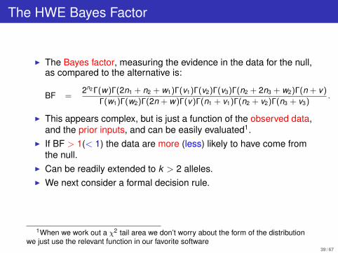
The HWE Bayes Factor

I The Bayes factor, measuring the evidence in the data for the null,as compared to the alternative is:

BF =2n2 Γ(w)Γ(2n1 + n2 + w1)Γ(v1)Γ(v2)Γ(v3)Γ(n2 + 2n3 + w2)Γ(n + v)

Γ(w1)Γ(w2)Γ(2n + w)Γ(v)Γ(n1 + v1)Γ(n2 + v2)Γ(n3 + v3).

I This appears complex, but is just a function of the observed data,and the prior inputs, and can be easily evaluated1.

I If BF > 1(< 1) the data are more (less) likely to have come fromthe null.

I Can be readily extended to k > 2 alleles.I We next consider a formal decision rule.

1When we work out a χ2 tail area we don’t worry about the form of the distributionwe just use the relevant function in our favorite software

39 / 67

Bayesian Decision Theory

I Decision as to reject H0 in favor of H1 depends on the costs ofmaking the two types of error:

DecisionReport H0 Report H1

H0 0 CITruthH1 CII 0

I Costs of making the two types of error CI is the cost of a type Ierror and CII the cost of a type II error.

I The decision theory solution is to report H1 if:

Posterior Odds of H0 = BF× Prior Odds <CII

CI= R

so that we only need to consider the ratio of costs R.I If CII

CI= 4 (type II errors four times as bad as type I errors) then

report H1 ifPosterior Odds of H0 < 4,

i.e. ifPr(H1| data ) > 0.2.

40 / 67

A Simple Example

We again consider the data n1 = 88,n2 = 10,n3 = 2.

These data give a p-value of 0.0654.

With “flat” conjugate Dirichlet priors (w1 = w2 = v1 = v2 = v3 = 1) weobtain a Bayes factor of 1.54 so that the data are 50% more likelyunder the null than the alternative, so the evidence in favor of H0 isnot strong.

With a prior probability of the null π0, to give a prior odds ofπ0/(1− π0), we have

Posterior Odds of H0 = BF× π0

1− π0.

Hence, with π0 = 0.5 the posterior odds equal the Bayes factor,i.e., 1.54.

41 / 67

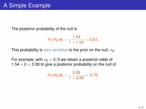
A Simple Example

The posterior probability of the null is

Pr(H0|n) =1.54

1 + 1.54= 0.61.

This probability is very sensitive to the prior on the null, π0.

For example, with π0 = 2/3 we obtain a posterior odds of1.54× 2 = 3.08 to give a posterior probability on the null of

Pr(H0|n) =3.08

1 + 3.08= 0.75.

42 / 67

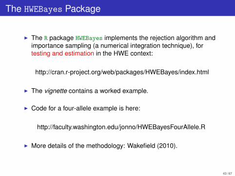
The HWEBayes Package

I The R package HWEBayes implements the rejection algorithm andimportance sampling (a numerical integration technique), fortesting and estimation in the HWE context:

http://cran.r-project.org/web/packages/HWEBayes/index.html

I The vignette contains a worked example.

I Code for a four-allele example is here:

http://faculty.washington.edu/jonno/HWEBayesFourAllele.R

I More details of the methodology: Wakefield (2010).

43 / 67

Poisson Modeling of Count Data

44 / 67

AIDS DataWhyte et al. (1987) reported deaths due to AIDS in Australian3-month periods from January 1983 to June 1986.

2 4 6 8 10 12 14

010

2030

4050

60

TIME

DE

ATH

S

Figure 11: AIDS death in Australia as a function of time.

45 / 67

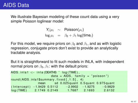
AIDS Data

We illustrate Bayesian modeling of these count data using a verysimple Poisson loglinear model:

Yi |µi ∼ Poisson(µi )

logµi = β0 + β1 log(timei )

For this model, we require priors on β0 and β1, and as with logisticregression, conjugate priors don’t exist to provide an analyticallytractable analysis.

But it is straightforward to fit such models in INLA, with independentnormal priors on β0, β1: with the default priors:

AIDS . i n l a 1 <− i n l a (DEATHS ˜ log (TIME ) ,data = AIDS , f a m i l y = ” poisson ” )

round ( AIDS . inla1$summary . f i x e d [ , 1 : 5 ] , 4)mean sd 0.025 quant 0.5 quant 0.975 quant

( I n t e r c e p t ) −1.9429 0.5112 −2.9902 −1.9275 −0.9829log (TIME) 2.1749 0.2149 1.7687 2.1693 2.6132

46 / 67

0.0 0.5 1.0 1.5 2.0 2.5

010

2030

4050

60

log(TIME)

DE

ATH

S

Figure 12: AIDS death in Australia as a function of time, with posterior mean(and 95% credible interval) of the expected value, Poisson model.

47 / 67

Negative Binomial Model

The Poisson model is often inadequate, as the variance isconstrained to equal the mean.

The negative binomial model adds an overdispersion parameter φ,such that

var(Yi ) = µi (1 + µi/φ),

to increase flexibility.

This model is also straightforward to fit in INLA:

AIDS . i n l a 2 <− i n l a (DEATHS ˜ log (TIME ) ,data = AIDS , f a m i l y = ” nb inomia l ” )

round ( AIDS . inla2$summary . f i x e d [ , 1 : 5 ] , 4)mean sd 0.025 quant 0.5 quant 0.975 quant

( I n t e r c e p t ) −2.0210 0.5784 −3.2318 −1.9965 −0.9527log (TIME) 2.2101 0.2491 1.7485 2.1998 2.7310

48 / 67

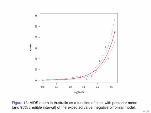
0.0 0.5 1.0 1.5 2.0 2.5

010

2030

4050

60

log(TIME)

DE

ATH

S

Figure 13: AIDS death in Australia as a function of time, with posterior mean(and 95% credible interval) of the expected value, negative binomial model.

49 / 67

Conclusions

HWE Example:

I The dirichlet distribution is convenient but quite inflexible as aprior distribution.

I Alternative priors are more difficult to specify since they are onscales that are more difficult to interpret (e.g. the logistic-normaldistribution) – see Appendix.

I For multiple alleles computation is slow whether the approach isfrequentist or Bayesian.

I On the course website there is Stan code to analyze multinomialdata, and this allows flexibility in prior specification.

50 / 67

Conclusions

Poisson/negative binomial example:

I Poisson and negative binomial models are straightforward to fitusing INLA.

I In fact, any generalized linear models (GLMs) are easy.

I In Lecture 7, we extend these models, to allow for randomeffects.

51 / 67

Conclusions

General Conclusions:

I In multiparameter situations, integration is required.

I INLA can perform the necessary integrations, and is fast andrelatively easy to use, though can’t be used for all models.

I Bayes factors are sensitive to the prior.

I Monte Carlo sampling is a powerful tool for inference.

52 / 67

References

Lidicker, W., William, Z., and McCollum, F. (1997). Allozymic variationin California sea otters. Journal of Mammalogy , 78, 417–425.

Shoemaker, J., Painter, I., and Weir, B. (1998). A bayesiancharacterization of hardy-weinberg disequilibrium. Genetics, 149,2079–2088.

Wakefield, J. (2010). Bayesian methods for examininghardy–weinberg equilibrium. Biometrics, 66, 257–265.

Wakefield, J. (2013). Bayesian and Frequentist Regression Methods.Springer, New York.

53 / 67

Appendix

54 / 67

Derivation of Bayes Factor for Assessing HWE

I We need to specify priors on the null and alternatives, and thencalculate the Bayes factor:

Pr(n|H0)

Pr(n|H1)=

∫Pr(n|p1)p(p1)dp1∫

Pr(n|q1,q2)p(q1,q2)dq1dq2

where p1 and (q1,q2) are the parameters under the null andalternative, respectively.

I Under the null we have a single parameter, and under thealternative two.

I Important point: When Bayes factors are evaluated we need toinclude the normalizing constants.

55 / 67

HWE Bayes Factor

I Under H0 and H1 we must take care to evaluate the probability ofthe same data, n1,n2,n3.

I Under the null,

Pr(n|p1) = Pr(n1,n2,n3|p1) =n!2n1

n2!n12!n3!p2n1+n2

1 (1− p1)n2+2n3 .

I With a Be(w1,w2) prior on p1:

Pr(n1,n2,n3|H0) =

∫Pr(n|p1)× p(p1)dp1

=n!2n2 Γ(w)Γ(2n1 + n2 + w1)Γ(n2 + 2n3 + w2)

n1!n2!n3!Γ(w1)Γ(w2)Γ(2n + w)

(2)

I This is the probability of the observed data under the null.

56 / 67

HWE Bayes Factor

I The Bayes factor isPr(n|H0)

Pr(n|H1)

and we have just given the form of the numerator.I We now turn to the denominator.I Under the alternative we assume q ∼ Dirichlet(v1, v2, v3).I The probability of the data under the alternative is:

Pr(n1,n2,n3|H1) =

∫Pr(n|q1,q2)× p(q1,q2)dq1dq2

=n!Γ(v)Γ(n1 + v1)Γ(n2 + v2)Γ(n3 + v3)

n1!n2!n3!Γ(v1)Γ(v2)Γ(v3)Γ(n + v).

(3)

I Again, just a probability distribution, which we may evaluate forany realization of (n1,n2,n3).

57 / 67

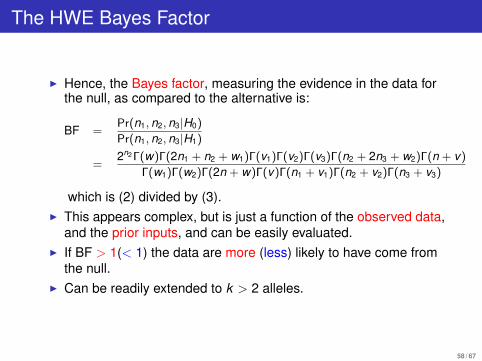
The HWE Bayes Factor

I Hence, the Bayes factor, measuring the evidence in the data forthe null, as compared to the alternative is:

BF =Pr(n1, n2, n3|H0)

Pr(n1, n2, n3|H1)

=2n2 Γ(w)Γ(2n1 + n2 + w1)Γ(v1)Γ(v2)Γ(v3)Γ(n2 + 2n3 + w2)Γ(n + v)

Γ(w1)Γ(w2)Γ(2n + w)Γ(v)Γ(n1 + v1)Γ(n2 + v2)Γ(n3 + v3)

which is (2) divided by (3).I This appears complex, but is just a function of the observed data,

and the prior inputs, and can be easily evaluated.I If BF > 1(< 1) the data are more (less) likely to have come from

the null.I Can be readily extended to k > 2 alleles.

58 / 67

A Non-Conjugate Test of HWE

The above prior specifications are convenient analytically, but in somesituations we would like to perform Bayesian inference using priorsthat are based on contextual information.

If we are really interested in the deviations from HWE of a samplefrom a particular population, then we may have strong priorinformation which perhaps can be represented through a prior on theinbreeding coefficient f .

59 / 67

A Different Prior for the Alternative

Under the null we have a single probability p1, the probability of an A1allele.

Under the alternative we may specify the prior

π(p1, f ) = π(p1)× π(f |p1)

where the conditioning allows the constraints on f :

fmin = max

(− p1

1− p1,−1− p1

p1

)< f < 1

Unfortunately there is no closed form calculations for finding posteriordistributions and Bayes factors, instead we describe asimulation-based technique —the rejection algorithm.

60 / 67

A Rejection Algorithm

Let θ denote the parameters with prior distribution π(θ), and let θ̂ bethe MLE and p(y |θ̂) the maximized likelihood.

Then the rejection algorithm (e.g., Wakefield, 2013, Chapter 3)proceeds as follows:

1. Generate U ∼ U(0,1) and θ ∼ π(θ), independently.2. Accept θ if

U <p(y |θ)

p(y |θ̂),

otherwise reject θ.3. Return to 1.

The resultant θ(s), s = 1, . . . ,S, are an independent sample from theposterior p(θ|y).

61 / 67

A Rejection Algorithm

The rejection algorithm may be very inefficient if the prior andlikelihood differ substantially (e.g., prior is dispersed and/or likelihoodis peaked).

An estimate of the normalizing constant (required for Bayes factorcalculation) is given by

p̂(y) =1S

S∑s=1

p(y |θ(s))

where θ(s) ∼ π(·).

Note that this only requires samples from the prior — the rejectionalgorithm is not needed.

In the HW context the maximized likelihood is available in closed form.

62 / 67

Specific Non-Conjugate Priors

Recall the prior isπ(p1, f ) = π(p1)× π(f |p1)

Two components:I For π(p1) we take a Be(w1,w2) prior.I For π(f |p1) we transform to

φ = log((f − fmin)/(1− f ))

and assume φ|p1 is normal.

63 / 67

HWE Example Revisited

We again consider the data n11 = 88,n12 = 10,n22 = 2.

These data give a p-value of 0.0654. The MLE for f is 0.23 withasymptotic standard error 0.17. MLE of HWE proportions:(0.865,0.130,0.05).

With flat conjugate Dirichlet priors we obtained a Bayes factor of 1.54so that the data are 50 % more likely under the null, but the evidenceis low.

64 / 67

HWE Example Revisited

We assume that the 50% point of the prior on f is 0, and the 95%point is 0.5

We obtain a Bayes factor of 0.29 so that the data are 3.4 times aslikely under the alternative, but the evidence is again weak.

The posterior probability that f > 0 is 0.98.

The difference between the priors is that the non-conjugate versiongives more weight close to where the data are located.

65 / 67

Graphical Summaries

●

●

●

●

●

●

●

●

●

●●

●

●

●

●

●

●

●

●

●●

●

●

●

●

●

●

●

●

●

●

●

●

●

●

●

●

●

●

●

●

●

●

●

●

●

●

●

●

●

●

●

●

●

●

●

●

●

●

●

●

●

●

●

●

●

●

●

●

●

●

●

●

●

●

●

●

●

●

●

●

●

●

●

●●

●

●

●

●

●

●

●

●

●

●

●

●

●

●

●

●

●

●

●

●

●

●

●

●

●

●

●

●

●

●

●

●

●

●

●

●

●

●

●

●

●

●

●

●

●

●

●

●

●

●

●

●

●

●

●

●

●

●

●

●

●

●

●

●

●

●

●

●

●

●

●

●

●

●

●

●

●

●

●

●

●

●

●

●●

●

●

●

●

●●

●

●

●

●

●

●

●

●

●

● ●

●

●

●

●

●

●

●●

●

●

●

●

●

●

●

●

●

●

●

●

●

●

●

●

●

●

●

●

●

●

●

●

●

●

●

●

●

●

●

●

●

●

●

●

●

●

●

●

●

●

●

●

●

●

●

●

●

●

●

●

●

●

●

●

●

●

●

●

●

●

●

●

●

●

●

●

●

●

●●

●

●

●

●

●

●

●

●

●

●

●

●

●

●

●

●

●

●

●

●

●

●

●

●

●

●

●

●

●

●

●

●

●

●

●

●

●

●

●

●

●

●

●

●

●

●

●

●

●

●

●

●

●

●

●

●

●

●

●

●

●

●

●

●

●

●

●

●

●

●

●

●

●

●

●

●

●

●

●

●

●

●

●

●

●

●

●

●

●

●

●

●

●

●

●

●

●

●

●

●

●

●

●

●

●

●

●

●

●

●

●

●

●

●

●

●

●

●

●

●

●

●

●

●

●

●

●

●

●

●

●

●

●

●

●

●

●

●

● ●

●

●

●●

●

●

●

●

●

●

●

●

●

●

●

●

●

●●

●

●

●

●

●

●

●

●

●

●

●

●

●

●

●

●

●

●

●

●

●

●

●

●

●

●

●

●

●

●

●

●

●

●

●

●

●

●

●

●

●

●

●

●

●

●

●

●

●

●

●

●

●

●

●

●

●

●

●

●

●

●

●

●

●

●

●

●

●

●

●

●

●

●

●

●

●

●

●

●

●

●

●

●

●

●

●

●

●

●

●

●

●

●

●

●

●

●

●

●

●

●

●

●

●

●

●

●

●

●

●

●

●

●

●

●

●

●

●

●

●

●

●

●

●

●

●

●

●

●

●

●

●

●

●

●

●

●

●

●

●

●

●

●

●

●

●

●

●

●

●

●

●

●

●

●

●

●

●

●

●

●

●●

●

●

●

●

●

●

●

●

●

●

●

●

●

●

●

●

●

●

●

●

●

●

●

●

●

●

●

●

●

●

●

●

●

●

●

●

●

●

●

●

●

●●

●

●

●

●

●

●

●

●

●

●

●●

●

●

●

●

●

●

●

●

●

●

●

●

●

●

●

●

●

●●

●

●

●

●

●

●

●

●

●

●

●

●

●

●

●

●

●

●

●

●

●

●

●

●

● ●

●

●

●

●

●

●●

●

●

●

●

●

●

●

●

●

●

●●

●

●

●

●

●

●●

●

●

●

●●

●

●

●

●

●

●

●

●

●

●

●

●

●●

●

●

●

●

●

●

●

●

●

●

●

●

●

●

●

●

●

●

●

●

●

●

●

●

●

●

●

●

●

●

● ●

●

●

●●

●

●

●

●

●

●

●

●

●

●

●

●

●

●

●

●

●

●

●●

●

●

●

●

●

●

●

●

●

●

●

●

●

●

●

●

● ●

●

●

●

●

●

●

●

●

●

●

●

●

●

●

●

●

●

●

●

●

●

●

●

●

●

●

●

●

●

●

●

●

●

●

●

●

●

●

●

●

●

●

●

●

●

●

●

●

●

●

●

●

●

●

●

●

●

●

●

●

●

●

●

●

●

●

●

●

●

●

●

●

●

●

●

●

●

●

●

●

●

●

●

●

●

●

●

●

●

●

●

●

●

●

●

●

●

●

●

●

●

●

●

●

●

●

●

●

●

●

●

●

●

●

●

●

●

●

●

●

●

●

●

●

●

●

●

●

●

●

●

●

●

●

●

●●

●

●

●

●

●

●

●

●

●

●

●

●

●

●

●

●

●

●

●

●

●

●

●

●

●

●

●

●

●

●

●

●

●

●

●

●

●

●

●

●

●

●

●

●

●

●

●

●

●

●

●

●

●

●

●

●

●

●

●

●

●

●

●

●

●

●

●

●

●

●

●

●●

●

●

●

● ●

●

●

●

●

●

●

●

●

●

●

●

●

●

●

●

●

●

●

●

●

●

●

●

●

●

●

●

●

●

●

●●

●

●

●

●

●

●

●

●

●

●

●

●

●

●

●

●

●

●

●

●

●

●

●

●

●

●

●

●

●

●

●

●

●

●

●

●●

●

●

●

●

●

●

●

●

●

●

●

●

●

●

●

●

●

●

●

●

●

●

●

●

●

●

●

●

●

●

●

●

●

●

●

●

●

●

●

●

●

●

●

●

●

●

●

●

●

●

●

●

●

●

●

●

●

●

●

●

●

●

●

●

●

●

●

●

●

●

●

●

●

●

● ●

●

●

●

●

●

●

●●

●

●

●

●

●

●

●

●

●

●

●

●

●

●

●

●

●

●

●

●

●

●

●

●

●

●

●

●

●

●

●

●

●

●

●

●●

●

●

●

●

●

●

●

●

●

●

●

●●

●

●

●

●

●

●

●

●

●

●

●

●

●

●

●

●

●

●

●

●

●

●●

●

●

●

●

●

●

●

●

●

●

●

●

●●

●

●

●

●

●

●

●

●

●

●

●

●

●

●

●

● ●

●

●

●

●

●

●

●

●

●

●

●

●

●

●

●

●

●

●

●

●

●

●

●

●

●

●

●

●

●

●

●

●

●

●

●

●

●

●

●

●

●

●

●

●

●

●●

●

●

●●

●

●

●

●

●

●

●

●

●

●

●

●

●

●

●

●

●

●

●

●

●

●

●

●

●

●

●

●

●

●

●

●

●

●

●

●

●

●

●

●

●

●●

●

●

●

●

●

●

●

●

●

●

●

●

●

●

●

●

●

●

●

●

●

●

●

●

●

●

●

●●

●

●

●

●●

●

●

●

●

●

●

●

●

●

●

●

●

●

●

●

●

●

●

●

●

●

●

●

●

●

●

●

●

●

●

●

●

●

●

●

●

● ● ●

●

●

●

●

●

●

●

●

●

●

●

●

●

●

●

●

●

●

●

●

●

●

●

●

●

●

●

●

●

●

●

●

●

●

●

●

●

●

●

●

●

●

●

●

●

●

●●

●

●

●

●

●

●

●

●

●

●

●

●

●

●●

●

●

●

●

●

●

●

●

●

●

●

●

●

●

●

●

●

●

●

●

●

●

●● ●

●

●

●

●

●

●

●

●

●

●

●

●

●

●

●

●

●●

●

●

●

●

●●

●

●

●

●

●

●

●

●●

●

●

●

●

●

●

●

●

●

●

●

●

●

●

●

●

●

●

●

●

●

●

●

●

●

●

●

●

●

●

●

●

●

●

●

●

●

●

●

●

●

●

●

●

●

●●

●●

●

●

●

●

●

●

●

●

●

●

●

●

●

●

●

●

●

●

●

●

●

●

●

●

●●

●●

●

●

●

●

●

●

●

●

●

●

●●

●

●●

●

●

●

●

●

●

●

●

●

●

●

●

●

●

●

●

●

●

●

●

●

●

●

●

●

●

●

●

●

●

●

●

●

●

●

●

●

● ●

●

●

●

●

●

●

●

●

●

●

●

●

●

●

●

●

●

●

●

●

●

●

● ●

●

●●

●

●

●

●

●

●

●

●

●

●

●

●

●

●

●

●

●

●

● ●

●

●

●

●

●

●

●

●

●

●

●

●

●

●

●

●

●

●

●

●

●

●

●

●

●

●

●●

●

●

●

●

●

●

●

●

●

●

●

●

●

●

●

●

●

●●

●

●

●

●

●

●

●

●

●

●

●

●

●

●

●

●

●

●

●

●

●

●

●

●

●

●

●

●

●

●

●

●

●

●

●

●

●

●

●

●

●

●

●

●

●

●

●

●

●

●

●

●

●

●

●

●

●

●

●

●

●

●

●

●

●

●

●

●

●

●

●

●

●

●

●

●

●

●

●

●

●

●

●

●

●

●

●

●

●

●

●

●

●

●

●

●

●

●

●

●

●

●

●

●

●

●

●

●

●

●

●

●

●

●

●

●

●

●

●

●

●

●

●

●

●

●

●

●

●

●

●

●

●

●

●

●

●

●

●

●

●

●

●

●

●

●

●

●

●●

●

●

●

●

●

●

●

●

●

●

●

●

●

●

●

●

●

●

●●

●

●

●

●

●

●

●

●

●

●

●

●

●

●

●

● ●

●

●

●

●

●

●

●

●

●

● ●

●

●

●

●

●

●

●

●

●

●

●

●

●

●

●

●

●

●

●

●

●

●

●

●

●

●

●

●

●

●

●

●

●

●

●

●

●

●

●

●

●

●

●

●

●

●

●

●

●

●

●

●

●

●

●

●

●

●

●

●

●

●

●

●

●

●

●

●

●

●

●

●

●

●

●

●

●

●

●

●

●

●

●

●

●

●

●

●

●

●

●

●

●

●

●

●

●

●

●

●●

●

●

●

●

●

●

●

●

●

●

●

●

●

●

●

●

●

●

●●

●

●

●

●

●

●

●

●

●

●

●

●

●

●

● ●

●

●

●

●

●

●

●

●

●

●

●

●

●

●

●

●

●

●

●

●

●

●

●

●

●

●

●

●

●

●

●

●

●

●

●

●

●●

●

●

●

●

●

●●

●

●

●

●

●

●

●

●

●

●

●

●

●

●

●

●

●

●

●

●

●

●

●

●

●

●

●

●

●

●

●

●

●

●

●

●

●●

●●

●

●

●

●

●

●

●

●

●

●

●●

●

●

●

●

●

●

●

●

●

●

●

●

●

●

●

●

●

●

●

●

●

●

●

●

●

●

●

●

●

●

●

●

●

●

●

●

●

●

●

●

●

●

●

●

●

●

●

●

●

●

●

●

●

●

●

●

●

●

●

●

●

●

●

●

●

●

●

●

●

●

●●

●

●

●

●

●

●

●

●

●

●

●

●

●

●

●

●

●

●

●

●

●

●

●

●

●

●

●

●

●

●

●

●

●

●

●

●

●

●

●

●

●

●

●

●

●

●

●

●

●

●

●

●

●

●

●

●

●

●

●

●

●

●

●

●

●

●

●

●

●

●

●

●

●

●

●

●

●

●

●

●

●

●

●

●

●

●

●

●

●

●

●

●

●●

●

●

●

●

●

●

●

●

●

●

●

●

●

●

●

●

●

●

●

●

●

●

●

●

●

●

●

●

●

●

●

●

●

●

●

●

●

●

●

●

●

●

●

●

●

●

●

●

●

●

●

●

●

●

●

●

●

●

●

●

●

●

●

●

●

● ●

●

●

●

●

●

●

●

●

●

●

●

●

●

●

●

●

●

●

●

●

●

●

●

●

●

●

●

●

●

●

●

●

●

●

●

●

●

●

●

●

●

●

●

●

●

●

●

●

●

●

●

●

●

●

●

●

●

●

●

●

●

●

●

●

●

●

●

●

●

●

●

●

●

●

●

●

●

●

●

●

●

●

●

●

●

●

●

●

●

●

●

●

●

●

●

●

●

●

●

●

●

●

●

●

●

●

●

●

●

●

●

●

●

●

●

●

●

●

●

●

●

●

●

●

●

●

●

●

●

●●

● ●

●

●

●

●

●

●

●

●

●

●

●

●

●

●●

●

●

●

●●

●

●

●

●

●●

●

●

●

●

●

●

●●

●

●

●

●

●

●

●

●

●

●

●

●

●

●

●

●

●

●

●

●

●

●

●

●

●

●

●

●

●

●

●

●

●

●

●

●

●

●

●

●

●

●

●

●

●

●

●

●

●

●

●

●

●

●

●

●

●

●

●

●

●

●

●

●

●

●

●

●

●

●

●

●

●

●

●

●

●

●

●

●

●

●

●

●

●

●

● ●

●

●

●

●●

●

●

●

●

●

●

●

●

●

●

●

●

●

●

●

●

●

●

●

●

●

●

●

●

●

●

●

●

●

●

●

●

●

●

●

●

●

●

●

●

●

●

●

●

●

●

●

●

●

●

●

●

●

●

● ●

●

●

●

●

●

●

●

●

●

●

●

●

●

●

●

●

●

●

●

●

●●

●

●

●

●

●

●

●

●

●

●

●

●

●

●

●

●

●

●

●

●

●

●

●

●

●

●

●

●

●

●

●

●

●

●●

●

●

●

●●

●

●

●

●

●

●

●

●

●

●

●

●

●

●

●

●

●

●

●

●

●

●

●

●

●

●

●

●

●

●

●

●

●

●

●

●●

●

●

●

●

●

●

●

●

●

●

●

●

●

●

●

●

●

●

●

●

●

●

●

●

●

●

●

●

●

●

●

●

●●

●

●

●

●

●

●

●

●●

●

●

●

●

●

●

●

●

●

●

●

●

●

●

●

●

●

●

●

●

●

●

●

●

●

●

●

●

●

●

●

●

●

●

●

●

●

●

●

●

●

●

●

●

●

●

●

●

●

●

●

●

●

●

●

●

●

●

●

●

●

●

●

●

●

●

●

●

●

●

●

●

●

●

●

●

●

●

●

●

●

●

●

●

●

●

●

●

●

●

●

●

●

●

●

●

●

●

●

●

●

●

●

●

●

●

●

●

●

●

●

●

●

●

●

●

●

●

●

●

●

●

●

●

●

●

●

●

●

●

●

●

●

●

●

●

●

●

●

●

●

●

●

●

●

●

●

●

●

●

●

●

●

●

●

●

●

●

●

●●

●

●

●

●

●

●

●

●

●

●

●

●

●

●

●

●

●

●

●

●

●

●

●

●

●

●

●

●

●

●

●

●

●●

●

●

●

●

●

●

●

●

●

●

●

●

●●

●

●

●

●

●

●

●

●

●

●

●

●

●

●

●

●

●

●

●

●

●

●

●

●

●

●

●

●

●

●

●

●

●

●

●

●

●

●

●

●

●

●

●

●

●

●

●

●

●

●

●

●

●

●

●

●

●

●

●●

●

●

●

●

●

●

●

●

●

●

●

●

●

●

●

●

●

●

●

●

●

●●●

●

●

● ●

●

●

●

●

●

●

●

●●

●

●

●

●

●

●

●

●

●

●

●

●

●

●

●

●

●

●

●

●

●

●

●

●

●

●

●

●

●

●

●

●

●●

●

●

●

●

●

●

●

●

●

●

●

●

●

●

●

●

●

●

●

●

●

●

● ●

●

●

●

●

●

●

●●

●

●

●

●

●

●

●

●

●

●

●

●

●

●

●

●

●

●

●

●

●

●

●

●

●

●

●

●

●

●

●

●

●

●

●

●

●

●

●

●

●

●

●

●

●

●

●

●

●

●

●

●

●

●

●

●

●

●

●

●

●

●

●

●

●

●

●

●

●

●

●

●

●

●

●

●●

●

●

●

●

●

●

●

●

●

●

●

●

●

●

●

●

●

●

●

●

●

●

●

●

●

●

●

●

●

●

●

●

●

●

●

●

●

●

●●

●

●

●

●

●

●

●

●

●

●

●

●

●

●

●

●

●

●

●

●

●

●

●

●●

●

●

●

●

●

●

●

●

●

●

●

●

●

●

●

●

●

●

●

●

●

●

●

●

●

●

●

●

●

●

●

●

●

●

●

●

●

●

●

●

●

●

●

●

●

●

●

●

●

●

●

●

●

●

●

●

●

●

●

●

●

●

●

●

●

●

●

●

●

●

●

●

●

●

●

●

●

●

●

●

●

●

●

●

●

●

●

●

●

●

●

●

●

●

●

●●

●

●

●

●

●

●

●

●

●

●

●

●

●

●

●

●

●

●

●

●

●

●

●

●

●

●

●

●

●

●

●

●

●

●

●

●

●

●

●

●

●

●

●

●

●

●

●

●

●

●●

●

●

●

●

●

●

●

●

●

●

●

●

●

●

●

●

●

●

●

●

●

●

●

●

●

●

●

●

●

●

●

●

●

●

●

●

●

●

●

●

●

●

●

●

●

●

●

●

●

●

●

●

●●

●

●

●

●

●

●

●

●

●

●

●

●

●

●

●

●

●

●

●

●

●

●

●

●

●

●

●

●

●

●

●

●

●

●

●

●

●

●

●

●

●

●

●

●●

●

●

●

●

●

●

●

● ●

●

●

●

●

●

●

●

●●

●

●

●

●

●

●

●

●

●

●

●

●

●●

●

●

●

●

●

●

●

●

●

●

●

●

●

●

●

●

●

●

●

●

●

●

●

●

●

●

●

●

●

●

●

●

●

●

●

●

●

●

●

●

●

●

●

●

●

●

●

●

●

●

● ●

●

●

●

●

●

●

●

●

●

●

●

●

●

●

●

●

●

●

●

●

●

●

●

●

●

●

●

●

●

●

●

●

●

●

●

●

●

●

●

●

●

●

●

●

●

●

●

●

●

●

●

●

●

●

●

●

●

●

●

●

●

●

●

●

●

●

●

●

●

●●

●●

●

●

●

●

●

●

●

●●

●

●

●

●

●

●

●

●

●

●

●

●

●

●

●

●

●

●

●

●

●

●

●

●

●

●

●

●

●

●

●

●

●

●

●

●

●

●

●

●

●

●

●

●

●

●

●

●

●

●

●

●

●

●

●

●

●

●

●

●

●

●

●

●

●

●

●

●

●

●

●

●

●

●

●

●

●

●

●

●

●

●

●

●

●

●

●

●

●

●

●

●

●

●

●

●

●

●

●

●

●●

●

●

●

●

●

●

●

●

●

●

●

●

●

●

●

●

●

●

●

●

●

●

●

●

● ●

●

●

●

●

●

●

●

●

●

●

●●

●

●

●

●

●

●

●

●

●

●

●

●

●●

●

●

●

●

●

●

●

●

●

●

●

●

●

●

●

●

●

●

●

●

●

● ●

●

●

●

●

●

●

●

●

●

●

●

●

●

●

●

● ●

●

●

●

●

●

●

●

●

●

●

●

●

●

●

●

●

●

●

●

●

●

●

●

●

●

●

●

●

●

●

●

●

●

●

●

●

●

●

●

●

●

●

●

●

●

●

●

●

●

●

●

●

●

●

●

●

●

●

●

●

●

●

●

●

●

●

●

●

●

●

●

●

●

●

●

●

●

●

●

●

●

●

●

●

●

●

●

●

●

●

●

●

●

●

●

● ●

●

●●

●

●

●

●

●

●

●

●

●

●

●

●

●

●

●

●

●

●

●

●

●

●

●

●

●

●

●

●

●

●

●

●

●

●

●

●

●

●

●

●

●

●

●

●

●

●

●

●●

●

●

●

●

●

●

●

●

●

●

●

●

●

●

●

●

●

●

●

●

●●

●

●

●

●

●

●

●

●

●

●

●

●

●

●

●

●●

●

●

●

●

●

●

●

●

●

●

●

●

●

●

●

●

●

●

●

●

●

●

●

●

●

●

●

●

●

●

●

●

●

●

●

●

●

●

●

●

●

●

●

●

●

●

●

●

●

●

●

●●

●

●

●

●

●

●

●

●

●

●

● ●

●

●

●

●

●

●

●

●

●

●

●

●

●

●

●

●

●

●

●

●

●

●

●

●

●

●

●

●

●

●

●

●

●

●

●

●

●

●

●

●

●

●

●

●

●

●

●

●

●

●

●

●

●

●

●

●

●

●

●

●

●

●

●

●

●

●

●

●

●

●

●

●

●

●

●

●

●

●

●

●

●

●

●

●

●

●

●

●●

●

●

●

●

●

●

●

●

●

●

●

●

●

●

●

●

●

●

●

●

●

●

●

●

●

●

●

●

●

●

●

●

●

●

●

●

●

●

●

●

●

●

●

●

●

●

●

●

●

●

●

●

●

●

●

●

●

●

●

●

● ●

●

●

●

●

●

●

●

●●

●

●

●

●

●

●●

●

●

●

●

●

●

●

●

●

●

●

●

●

●

●

●

●

●

●

●

●●

●

●

●

●

●

●

●

●

●

●

●

●

●

●

●

●

●

●

●

●

●

●

● ●

●

●

●

●

●

●

●

●

●

●

●

●

●

●

●

●

●

●

●

●

●

●

●

●

●

●

●

●

●

●

●

●

●

●

●

●

●

●

●

●

●

●

●

●

●

●

●

●

●

●

●

●

●

●

●

●

●

●

●

●

●

●

●

●

●

●

●

●

●

●

●

●

●

●

●

●

●

●

●

●

●

●

●

●

●

●

●

●

●

●

●

●

●

●

●

●

●

●

●

●

●

●

●

●

●

●

●

●

●

●

●

●

●

●

●

●

●

●

●

●

●

●

●

●

●

●

●

●

●

●

●

●

●

●

●

●

●

●

●

●

●

●

●

●

●

●

●

●

●

●

●

●

●

●

●

●

●

●

●

●

●

●

●

●

●

●

●

●

●

●

●

●

●

●

●

●

●

●

●

●

●

●

●

●

●

●

●

●

●

●

●

●

●

●

●

●

●

●

●

●

●

●

●

●

●

●

●

●

●

●●

●

●

●

●

●

●●

●

●

●

●

●

●

●

●

●

●

●

●

●

●

●

●

●

●

●

●

●

●

●

●

●

●

●

●

●

●

●

●

●

●

●

●

●

●

●

●

●

● ●

●

●

●

●

●

●

●

●

●

●

●

●

●

●

●

●

●

●

●

●

●

●

●

●

●

●

●

●

●

●

●

●

●

●

●

●

●

●

●

●

●

●

●

●

●

●

●

●

●

●

●

●

●

●

●

●

●

●

●

●

●

●

●

●

●

●

●

●

●●

●

●

●

●

●

●

●

●

●

●

●

●

●●

●

●

●

●

●

●

●

●

●

●

●

●

●

●

●

●

●

●

●

●

●

●

●

●

●

●

●

●

●

●

●

●

●

●

●●

●

●

●

●

●

●

●

●

●

●

●

●

●

●

●

●

●

●

●

●

●

●

●

●

●

●

●

●

●

●

●

●

●

●

●

●

●

●

●

●

●

●

● ●

●

● ●

●

●

●

●

●

●

●

●

●

●

●

●

●

●

●

●

●

●

●

●

●

●●

●

●●

●

●

●

●

●

●

●

●●

●

●●

●

●

●

●

●

●

●

●

●

●

●

●

●

●

●

●

●

●

●

●

●

●

●

●

●

●

●

●

●

●

●

●

●

●

●

●

●

●

●

●●

●

●

●

●

●

●

●

●

●

●

●

●

●

●

●●

●

●

●

●

●

●

●

●

●

●

●

●

●

●

●

●

●

●

●

●

●

●

●

●

●

●

●

●

●

●

●

●

●

●

●

●

●

●

●

●

●

●

●

●

●

●

●

●

●

●

●

●

●

●

●

●

●

●

●

●

●

●

●

●

●

●

●

●

●

●

●

●

●

●

●

●

●

●

●

●

●

●

●

●

●

●

●

●

● ●

●

●

●

●

●

●

●

●

●

●

●

●

●

●

●

●

●

●

●

●

●

●

●

●

●

●

●

●

●

●

●

●

●

●

●

●

●

●

●

●

●

●

●

●

●

●

●

●

●

●

●

●

●

●

●

●

●

●

●

●

●

●●

● ●

●

●

●

●

●

●

●

●

●

●

●

●

●

●

●

●

●

●

●

●

●

●

●

●

●

●

●

●

●

●

●

●

●

●

●

●

●

●

●

●

●

●

●

●

●

●

●

●

●

●

●

●

●

●

●

●

●

●

●

●

●

●

●

●

●

●

●

●

●

●

●

●

●

●

●

●

●

●

●

●

●

●

●

●

●

●

●

●

●

●

●

●

●

●

●

●

●

●

●

●

●

●

●

●

●

●

●

● ●

●

●●

●

●

●

●

●

●

●

●

●

●

●

●

●

●

●

●

●

●

●

●

●

●

●

●

●

●

●

●

●

●

●

●

●

●

●

●

●

●

●

●

●

●

●

●

●

●

●

●

●

●

●

●

●

●

●

●

●

●

●

●

●

●

●

●

●

●

●

●

●

●

●

●

●

●

●

●

●

●

●

●

●

●●

●

●

●

●

●

●

●

●

●

●

●

●●

●●

●

●

●

●

●●

●

●

●

●

●

●

●

●

●

●

●

●

●

●

●

●

●

●

●

●

●

●

●

●

●

●

●

●

●

●

●

●

●

●

●

●

●●

●

●

●

●

●

●

●

●

●

●

●

●

●

●

●

●

●

●

●

●

●

●

●

●

●

●

●

●

●

●

●

●

● ●

●

●

●

● ●

●

●

●

●

●

●

●●

●

●

●

●

●

●

●

●

●

●

●

●

●

●

●

●

●

●

●

●

●

●

●

●

●

●

●

●

●

●

●

●

●

●

●

●

●

●

●

●

●

●

●

●

●

●

●

●

●

●

●

●

●

●

●

●

●

●

●

●

●

●

●

●

●

●

●

●

●

●

●

●

●

●

●

●

●

●

●

●

●

●

●

●

●

●

●

●

●

●

●

●

●

●

●

●

●

●

●

●

●

●

●

● ●

●

●

●

●

●

●

●

●

●

●

●

●

●

●

●

●●

●

●

●●

●

●

●

●

●

●

●

●

●

●●

●

●

●

●

●

●

●

●

●

●

●

●

●

●

●

●

●

●

●

●

●

●

●

●

●

●

●●

●

●

●

●

●

●

●●

●

●

●

●

●

●

●

●

●

●

●

●

●

●

●

●

●

●

●●

●

●

●

●

●

●

●

●

●

●

●

●

●

●

●

●

●

●

●

●

●

●

●

●

●

●

●

●

●

●

●

●

●

●

●

●

●

●

●

●

●

●

●

●

●

●

●●

●

●

●

●

●

●

●

●

●

●

●

●

●

●

●

●

●

●

●

●

●

●

●

●

●

●

●

●

●

●

●

●

●

●

●

●

●

●

●

●

●

●

●

●

●

●

●

●

●

●

●

●

●

●

●

●

●

●

●

●

●

●

●

●

●

●

●

●

●

●

●

●

●

●

●

●

●

●

●

●

●

●

●

●

●

●

●●

●

●

●

●

●

●

●

●

●

●

●

●

●

●

●

●

●

●

●

●

●

●

●

●

●

●●

●

●

●

●

●

●

●

●

●

●

●

●

●

●

●

●

●

●

●

●

●

●

●

●

●

●

●

●

●

●

●

●

●

●

●

●

●

●

●

●

●

●

●

●

●

●

●

●

●

●

●

●

●

●

●

●

●

●

●

●

●●

●

●

●

●

●

●

●

●

●

●

●

●

●

●

●

●

●

●

●

●

●

●

●

●

●

●

●

●

●

●

●

●●

●

●

●

●

●

●

●

●

●

●

●

●

●

●

●

●

●

●

●

●

●

●

●

●

●

●

●

●

●

●

●

●

●

●●

●

●

●

●

●

●

●

●

●

●

●

●

●

●

●●

●

●

●

●

●

●

●

●

●

●

●

●

●

●

●

●

●

●

●

●

●

●

●

●

●

●

● ●

●

●

●

●

●

●

●

●

●

●

●

●

●

●

●

●

●

●

●

●

●

●

●

●

●

● ●

●

●

●

●

●

●

●

●

●

●

●

●

●

●

●

●

●

●

●

●

●

●

●

●

●

●

●

●

●

●

●

●

●

●

●

● ●

●

●

●

●

●

● ●

●

●

●

●

●

●

●

●

●

●

●

●

●

●

●

●

●

●

●

●

●

●

●

●

●

●

●

●

●

●

●●

●

●

●

●

●

●

●

●

●

●

●

●

●

●

●

●

●

●

●

●

●

●

●

●

●

●

●

●

●

●

●●

●

●

●

●

●

●

●

●

●

●●

●

●

●

●

●

●

●

●

●

●

●

●

●

●

●

●

●

●

●

●

●

●

●

●

●

●

●

●

●

●

●

●

●

●

●

●

●

●

●

●

●

●

●

●

●

●

●

●

●

●

●

●

●

●

●

●

●

●

●

●

●

●

●

●

●

●

●

●

●

●

●

●

●

●

●

●

●

●

●

●

●

●

●

●

●

●

●

●

●

●

●

●

●

●

●

●

●

●

●

●

●

●

●

●

●

●

●

●

●

●

●

●

●

●

●

●

●

●

●

●

●

●

●

●

●

●

●

●

●

●

●

●

●

●

●

●

●

●

●

●

●

●

●

●

●

●

●

●

●

●

●

●

●

●

●

●

●

●

●

●

●

●

●

●

●

●

●

●

●

●

●

●

●

●

●

●

●

●

●

●

●

●

●

●

●

●

●

●

●

●

●

●

●

●

●

●

●

●

●

●

●

●

●

●

●

●

●

●

●

●

●

●

●

●

●

●

●

●

●

●

●

●

●

●

●

●

●

●

●

●

●

●

●

●

●

●

●

●

●

●

●

●

●

●

●

●

●

●

●

●

●

●

●

●

●

●

●

●

●

●

●

●

●

●

●

●

●

●

●

●

●

●

●●

●

●

●

●

●

●

●

●

●

●

●

●

●

●●

●

●

●

●

●

●

●

●

●

●

●

●

●

●

●

●

●

●

●

●

●

●

●

●

●

●

●

●

●

●

●

●

●

●

●●

●

●●

●

●

●

●

●

●

●

●

●

●

●

●

●

●

●

●

●

●

●

●

●

●

●

●

●

●

●

●

●

●

●

●

●●

●

●

●

●

●

●

●

●

●

●

●

●

●

●

●

●

●

●

●

●

●

●

●

●

●

●

●

●

●

●

●

●

●

●

●

●

●

●

●

●

●

●

●

●

●

●

●

●

●

●

●

●

●

●

●

●

●

●

●

●

●

●

●

●

●

●

●

●

●

●

●

●

●

●

●

●

●

●

●

●

●

●

●

●

●

●

●

●

●

●

●

●

●

●

●

●

●

●

●

●

●

●

●

●

●

●

●

●

●

●

●

●

●

●

●

●

●

●

●

●

●

●

●

●

●

●

●

●

●

●

●

●

●

●

●

●

●

●●

●

●

●

●

●

●

●

●

●

●

●

●

●

●

●

●

●

●

●

●

●

●

●

●

●

●

● ●

●

●

●

●

●

●

●

●

●

●

●

●

●●

●

●

●

●

●

●

●

●

●

●●

●

●

●

●

●

●

●

●

●

●

●

●●

●

●

●

●

●

●

●

●

●

●

●

●

●

●

●

●

●

●

●

●

●

●

●

●

●

●

●

●

●

●

●

●

●

●

●

●

●

●

●●

●

●

●

●

●

●

●

●

●

●

●

●

●

●

● ●

●

●

●

●

●

●

●

●

●

●

●

●

●

●

●

●

●

●

●

●

●

●

●

●

●

●

●

●

●

●

●

●

●

●

●

●

●

●

●

●

●

●

●

●

●

●

●

●

●

●

●

●

●

●

●

●

●

●

●

●

●

●

●

●

●

●

●

●

●

●

●

●

●

●

●

●

●

●

●

●●

●

●

●

●

●

●

●

●

●

●

●

●

●

●

●

●

●

●

●

●

●

●

●

●

●

●

●

●

●

●●

●

●

●

●

●

●

●

●

●

●

●

●

●

●

●

●

●

●

●

●

●

●

●

●

●

●

●

●

●

●

●

●

●

●

●

●

●

●

●

●

●

●

●

●

●

●

●

●

●

●

●

●

●

●

●

●

●

●

●

●

●

●

●

●

●

●● ●

●

●

●

●

●

●

●

●

●

●

●

●

●

●

●

●

●

●

●

●

●

●

●

●

●

●

●

●

●

●

●

●

●

●

●●

●

●

●

●

●

●

●

●

●

●

●

●

●

●

● ●

●

●

●

●

●

●

●

●

●

●

●

●

●

●

●

●

●

●

●

●

●

●

●

●

●

●

●

●

●

●

●

●

●

●

●

●

●

●

●

●

●

●

●

●

●

●

●

●

●

●

●

●

●

●

●

●

●

●

●

●

●

●

●

●

●

●

●

●

●

●

●●

●●

●

●

●

●

●

●

●

●

●

●

●

●

●

●

●

●

●

●

●

●

●

●

●

●

●●

●

●

●

●

●

●

●

●

●

●

●

●

●

●

●

●

●

●

●

●

●

●

●

●

●

●

●

●

●

●

●

●

●

●

●

●

●

●

●

●

●

●

●

●

●

●

●

●

●

●

●

●

●

●

●

●

●

●

●

●

●

●

●

●

●

●

●

●

●

●●

●

●

●

●

●

●

●

●

●

●

●

●

●

●

●

●

●

●

●

●

●

●

●

●

●

●

●

●

●

●

●

●

●

●

●

●

●

●

●

●

●

●

●

●

●

●

●

●

●

●

●● ●

●

●

●

●

●

●

●

●

●

●

●

●

●

●

●

●

●

●

●

●

●

●

●

●

●

●

●

●

●

●

●

●

●

●

●

●

●

●

●

●

●

●

●

●

●

●

●

●

●

●

●

●

●

●

●

●

●

●

●

●

●

●

●

●

●

●

●

●

●

●

●

●

●

●

●

●

●

●

●

●

●

●

●

●

●

●

●

●

●

●

●

●

●

●

●

●

●

●

●

●

●

●

●

●

●

●

●

●

●

●

●

●

●

●

●

●

●

●

●

●

●

●

●

●

●

●

●

●

●

●

●

●

●

●

●

●

●

●

●

●

●

●

●

●

●

●

●

●

●

●

●

●

●

●

●

●

●●

●

●

●

●

●

●

●

●●

●

●

●

●

●

●

●

●

●

●

●

●

●

●

●

●

●

●

●

●

●

●

●

●

●

●

●

●

●

●●

●

●

●

●●

●

●

●

●

●

●

●

●

●

●

●

●

●

●

●

●

●

●

● ●

●

●

●

●

●

●

●

●

●

●

●

●

●

●

●●

●

●

●

●

●

●

●

●

●

●●

●

●

●

●

●

●

●

●

●

●

●

●

●

●

●

●

●

●

●

●

●

●

●

●

●

●

●

●●

●

●

●

●

●

●

●

●

●

●

●

●

●

●

●

●

●

●

●

●

●

●

●

●

●

●

●

●

●

●

●

●

●

●

●

●

●

●

●

●

●

●

●

●

●

●

●

●

●

●

●

●

●

●

●

●

●

●

●

●

●

●

●

●

●

●

●

●

●

●

●●

●

●

●

●

●

●

●

●

●

●

●

●

●

●

●

●

●

●

●

●

●

●

●

●

●

●

●

●

●

●

●

●

●

●

●

●

●

●

●

●

●

●

●

●

●

●

●

●

●

●

●

●

●

●

●

●

●

●

●

●

●

●

●

●

●

●

●

●

●●

●

●

●

●

●

●

●

●

●

●

●

●

● ●

●●

●

●

●

●

●

●

●

●

●

●

●

●

●

●

●

●

●

●

●

●

●

●

●

●●

●

●

●

●

●

●

●

●

●

●

●

●

●

●

●

●

●

●

●

●●

●

●

●

●

●

●

●

●

●

●

●

●

●

●

●

●

●

●

●

●

●

●

●

●

●

●

●

●

●

●

●

●

●

●

●

●

●

●

●

●

●

●

●

●

●

●

●

●

●

●

●

●

●

●

●

●

●

●

●

●

●

●

●

●

●

●

●

●

●

●

●

●

●

●

●

●

●

●

●

●

●

●

●

●

●

●

●

●

●

●

●

●

●

●

●

●

●

●

●

●

●

●●

●

●

●

●

●

●

●

●

●

●

●

●

●

●

●

●

●

●

●

●

●

●

●

●

●

●

●

●

●

●

●●

●

●

●

●

●

●

●

●

●

●

●

●

●

●

●

●

●

●

●

●

●

●

●

●

●

●●

●

●

●

●

●

●

●

●

●

●

●

●

●

●

●

●

●

●

●

●

●

●

●

●

●

●

●

●

●

●

●

●

●

●

●

●

●

●

●

●

●

●

●

●

●

●

●

●

●

●

●

●

●

●

●

●

●

●

●

●

●

●

●

●

●

●

●

●

●

●

●

●

●

●

●

●

●

●

●

●

●

●

●

●

●

●

●

●

●

●

●

●●

●

●

●

●

●

●

●

●

●

●

●

●

●●

●

●

●

●

●

●

●

●

●

●

●

●

●

●

●

●

●

●

●

●

●

●

●

●

●

●

●

●

●

●

●

●

●

●

●

●

●

●

●

●

●

●

●

● ●

●

●

●

●

●

●

●

●

●

●

●

●

●

●

●

●

●

●

●

●

●

●

●

●

●

●

●

●

●

●

●

●

●

●

●

●

●

●

●

●

●

●

●

●

●

●

●

●

●

●

●●

●

●

●

●

●

●

●

●

●

●

●

●

●

●

●

●

●

●

●

●

●

●●

●

●

●

●

●

●

●

●

●

●

●

●

●●

●

●

●

●

●

●

●

●

●

●

●

●

●

●

●

●

●

●●

●

●

●

●

●

●

●

●

●

●

●

●

●

●

●

●

●

●

●

●

●

●

●

●

●

●

●●

●

●

●

●

●

●

●

●

●

●

●

●

●

●

●

●

●

●

●

●

●

●

●

●

●

●

●

●

●

●

●

●

●

●

●

●

●

●

●

●

●

●

●

●

●

●

●

●

●

●

●

●

●

●

●

●

●

●

●

●

●

●

●

●

●

●

●

●

●

●

●

●

●

●

●

●

●

●

●

●

●

●

●

●

●

●

●

●

●

●

●

●

●

●

●

●

●

●

●

●

●

●

●

●

●

●

●

●

●

●

●

●

●●

●

●

●

●

●

●

●

●

●

●

●

●

●

●

●

●

●

●

●

●

●

●

●

●

●

●

●

●

●●●

●

●

●

●

●

●

●

●

●

●

●

●

●

●

●

●

●

●

●

●

●

●

●

●

●

●

●

●

●

●

●

●

●

●

●

●

●

● ●

●

●

●

●

●

●

●

●

●

●

●

●

●

● ●

●

●

●

●

●

●

●

●

●

●

●

●

●

●

●

●

●

●

●

●

●

●

●

●

●

●

●

●

●

●

●

●

●

●

●

●

●

●

●

●

● ●

●

●

●

●

●

●

●

●

●

●

●

●

●

●

●

●●

●

●

●

●

●

●

●

●

●

●

●

●

●

●

●

●

●

●

●

●

●

●

●

●

●

●

●

● ●

●

●

●

●

●

●

●

●

●

●

●

●

●

●

●

●

●

●

●

●

●

●

●

●

●

●

●

●

●

●

●

●

●

●

●

●

●

●

●

●

●

●

●

●

●

●

●

●

●

●

●

●

●

●

●

●

●

●

●

●

● ●

●

●

●

●

●

●

●

●

●

●

●

●

●

●

●

●

●

●

●

●

●

●

●

●

●

●

●

●

●

●

●

●

●

●

●

●

●

●

●

●

●

●

●

●

●

●

●

●

●

●

●

●

●

●●

●

●

●

●

●

●

●

●

●

●

●

●

●

●

●

●

●

●

●

●

●

●

●

●

●

●

●

●

●

●

●

●

●

●

●

●

●

●

●

●

●

●

●

●

●

●

●

●

●

●

●

●

●

●

●

●

●

●

●

●

●

●

●

●

●

●

●

●

●

●

●

●

●

●

●

●

●

●

●

●

●

●

●

●

●

●

●

●

●

●

●

●

●

●

●

●

●

●

●

●

●

●

●

●

●

●

●

●

●

●

●

●

●

●

●

●

●

●

●●

●

●

●

●

●

●

●

●

●

●

●

●

●

●

●

●

●

●

●

●

●

●

●●●

●

●

●

●

●

●

●

●

●

●

●●

●

●

●

●

●●

●●

●

●

●

●

●

●

●

●

●

●

●

●

●

●

●

●

●

●

●

●

●

●

●

●

●

●

●

●

●

●

●

●

●

●

●

●

●

●

●

●

●

●

●

●

●

●

●

●

●

●

●

●

●●

●

●

●

●

●

●

●

●

●

●

●

●

●

●

●

●

●

●

●

●

●

● ●

●

●

●

●

●

●

●

●

●

●

●

●

●

●

●

●

●

●

●

●

●

●

●

●

●

●

●

●

●

●

●

●

●

●

●

●

●

●

●

●

●

●

●

●

●

●

●

●

●

●

●

●

●

●

●

●

●

●

●

●

●

●

●

●

●

●

●

●

●

●

●

●

●

●

●

●

●

●

●

●

●

●

●

●

●

●

●

●

●

●

●

●

● ●

●

●

●

●

●

●

●

●

●

●

●

●

●

●

●

●

●

●

●

●

●

●

●

●

●

●

●

●

●

●

●

●

●

●

●

●

●

●

●

●

●

●

●

●

●

●

●

●

●

●

●

●

●

●

●

●

●

●

●

●

●

●

●

●

●

●

●

●

●

●

●

●

●

●

●

●

●

●

●

●

●

●

●

●

●

●

●

●

●

●

●

●●

●

●

●

●

●

●

●

●

●

●

●

●

●

●

●

●

●

●

●

●

●

●

●

●

●

●

●

●

●

●

●

●

●●

●

●

●●

●

●

●

●

●

●

●

●

●

●

●

●

●

●

●

●

●

●

●

●

●

●

●

●

●

●

●

●

●

●

●

●

●

●

●

●

●

●

●

●

●

●

●

●

●

●

●

●

●

●

●

●

●

●

●

●

●

●

●

●

●

●

●

●

● ●

●

●

●

●

●

●

●

●

●

●

●

●

●

●

●

●

●

●

●

●

●

●

●

●

●

●

●

●

●

●

●

●

●●

●

● ●

●

●

●

●

●

●

●

●

●

●

●

●

●

●

●

●

●

●

●

●

●

●

●

●

●

●

●

●

●

●

●

●●

●

●

●

●

●

●

●

●

●

●

●

●

●

●

●

●

●

●

●

●

●

●

●

●

●

●

●

●

●

●

●

●

●

●

●

●

●

●

●

●

●

●

●●

●

●

●

●

●

●

●

●

●

●

●

●

●

●

●

●

●

●

●

●

●

●

●

●

●

●

●

●

●

●

●

●

●

●

●

●

●

●

●

●

●

●●

●

●●

●

●

●

●

●

●

●

●

●

●

●

●

●

●

●

●

●

●

●

●

●

●

●

●

●

●

●

●

●

●

●

●●

●

●●

●

●

●

●

●

●

●

●

●

●

●

●

●

●

●

●

●

●

●

●

●

●

●

●

●

●

●

●

●

●

●

●

●

●

●

●

●

●

●

●

●

●

●

●

●

●

●●

●

●

●

●

●

●

●

●

●

●

●

●

●

●

●

●

●

●

●

●●

●

●

●

● ●

●

●

●

●

●

●

●

●

●

●

●

●

●

●

●

●

●

●

●

●

●

●

●

●

●

●

●

●

●

●

●

●

●

●

●

●

●

●

●

●

●

●

●

●

●

●

●

●

●

●

●

●

●

●

●

●

●

●●

●

●

●

●

●

●

●

●

●

●

●

●

●

●

●

●

●

●

●

●

●

●

●

●

●

●

●

●

●

●

●

●

●

●

●

●

●

●

●

●

●

●

●

●

●

●

●

●

●

●

●

●

●

●

●

●

●

●

●

●

●

●

●

●

●

●

●

●

●

●

●

●

●

●

●

●

●

●

●

●

●

●

●

●

●

●

●

●

●

●

●

●

●

●

●

●

●

●

●

●

●

●

●

●

●

●

●

●

●

●

●

●

●

●

●●

●

●

●

●

●

●

●

●

●

●

●

●

●

●

●

●

●

●

●

●

●

●

●

●

●

●

●

●

●

●

●

●

●

●

●

●

●

●

●

●

●

●

●

●

●

●

●

●

●

●

●

●

●

●

●

●

●

●

●

●

●

●

●

●

●

●

●

●

●

●

●

●

●

●

●

●

●

●

●

●

●

●

●

●

●

●

●

●

●

●

●

●

●

●

●

●

●

●

●

●

●

●

●

●

●

●

●

●

●

●

●

●●

●

●

●

●

●

●

●

●

●

●

●

●

●●

●●

●

●

●

●

●

●

●

●

●

●

●

●

●

●

●

●

●

●

●

●

●

●

●

●

●

●

●

●

●

●

●

●

●

●

●

●

●

●

●

●

●

●

●

●

●

●

●

●

●

●

●

●

●

●

●

●

●

●

●

●

●

●

●

●

●

●

●

●

●

●

●

●

●

●

●

●

●

●

●

●●

●

●

●

●

●

●

●

●

●

●

●

●

●

●

●

●

●●

●

●

●

●

●

●

●

●

●

●

●

●

●

●

●

●

●

●

●

●

●

●

●

●

●

●

●

●

●

●

●

●

●

●

●

●

●

●

●

●

●

●

●

●

●

●

●

●

●

●

●

●

●

●

●

●

●

●

●

●

●

●

●

●

●

●

●

●

●

●

●

●

●

●

●

●

●

●

●

●

●

●

●

●

●

●

●

●

●

●

●

●

●

●

●

●

●

●

●

●

●

●

●

●

●●

●

●

●

●

●

●

●

●

●

●

●

●

●

●

●

●

●

●

●

●

●

● ●

●

●

●

●

●●

● ●

●

●

●

●

●

●

●

●

●

●

●

●

●

●

●

●

●

●

●

●●

●

●

●

●

●

●

●

●

●

●

●

●

●

●

●

●

●

●

●

●

●

●

●

●

●

●

●

●

●

●

●

●●

●

●

●

●

●

●

●

●

●

●

●

●

●

●

●

●

●

●●

●

●

●

●

●

●

●

●

0.0 0.2 0.4 0.6 0.8 1.0

−1.0

−0.5

0.00.5

1.0

p1

f

p1

Freque

ncy

0.0 0.2 0.4 0.6 0.8 1.0

0100

200300

400500

f

Freque

ncy

−1.0 −0.5 0.0 0.5 1.0

0500

1000

●

●

●

●

●

●●

●

●

●

●

●

●

●

●

●

●

●

●

●

●

●

●

●

●●

●

●

●

●

●

●

●

●

●

●

●

●

●

●

●

●●

●

●

●

●

●

●

●

●

●

●

●●

●

●

●

●

●

●

●

●●

●

●

●

●

●

●

●

●

●

●

●

●

●

●

●

●

●

●

●

●

●

●

●

●

●

●

●

●

●

●

●

●

●

●

●

●

●

●

●

●

●

●

●

●

●

●

●

●

●

●●

●

● ●

● ●

●

●

●

●

●

●

●

●

●

●

●

●

●

●

●

●

●

●●

●

●

●

●

●

●●

●

●●

●

●

●

●

●

●

●

●

●

●

●

●

●●

●

●

●

●

●

●

●

●

●

●●

●

●

●

●

●

●

●●

●

●●

●

●

●●

●

●

●

●

●

●●

●

●

●

●

●

●

●

●

●

●

●●

●

●

●

●

●

●

●

●

●

●

●

●

●

●

●

●

●

●

●

●

●

●

●

●

●

●

●

●

●

●

●

●

● ●●

●

●

●

●

●

●

●

●

●

●

●

●●

●●

●

●

●

●

●

●

●

●

●

●●

●

● ●

●

●

●

●

●

●

●

●

●

●

●●

●

●●

●

●

●●

●

●

●

●

●

●●

●

●

●

●

●

●

●

●

●

●

●

●

●

●

●

●

●

●

●

●

●

●

●

●

●

●

●

●

●

●

●

●

●

●

●

●●

●

●

●

●

●

●

●

●

●

●

●

●

●

●

●

●

●

●

●

●

●

●

●

●

●

● ●●

●

●

●

●

●

●

●

●

●

●

●

●

●

●

●

●

●

●

●

●

●

● ●

●

●

●

●

●

●

●●

●

●

●

●●

●

●

●

●

●

●

●

●

●

●

●

●

●●

●

●

●

●

●

●

●

●

●

●

●●

●

●

●

●

●

●

●

●

●

●

●

●

●

●

●

●

●

●●

●

●●

●●

●

●

●

●

●

●

● ●

●

●

●

●

●

●

●

●

●

●

●

● ●●

●

●

●

●

●

●●

●

●

●

●

●

●

●

●

●

●●

●

●

●

●

●

●

●

●

●

●

●

●

●

●

●

●

●

●

●

●

●

●

●

●

●

●

●

●

●

●

●

●

●

●

●

●

●

●

●

●

●●

●●

●

●

●

●

●

●

●

●

●

●

●●

●

●

●

●

●●

●

●

●

●

●

●

●

●

●

●

●

●

●

●

●

●

●

●

●

●●

●

●

●●

●

●

●

●

●

●

●

●

●

●

●

●

●

●

●

●

●

●

●

●

●

●

●

●

●

●

●

●

●

●

●

●

●

●

●

●●

●

●

●●

●

●

●

●

●

●

●

●

●

●

●●

●

●

●

●

●

●

●

●

●

●

●

●

●

●

●

●

●

●

●

●

●

●

●

●

●

●

●

●

●

●

●

●

●

●

●

●

●

●

●

●

●

●

●

●

●

●

●

●

●

●

●●●

●

●

●

●

●

●

●

●

●

●●

●

●

●

●

●

●

●

●

●●

●

●

●

●

●

●

●

●

●

●

●

●

●

●

●

●

●

●

●

●

●

●

●

●

●

●

●

●

●

●

●

●

●

●

●

●

●

●

●

●

●

●

●

●

●

●

●

●

●

●●

●

●●

●

●

●

●

●

●

●

●

●

●●

●

●

●

●

●●

●

●

●

●

●

●

●

●●

●

●

●

●●

●

●

●●●

●

●

●

●

●

●

●

●

●

●

●

●

●

●●

●

●

●●

●

●

●●

●

●

●

●

●

●

●

●

●

●

●

●

●

●

●

●

●

●

●

●

●

●

●

●

●

●

●

●

● ●

●

●

●

●

●

●

●

●

●

●

●●

●

●

●

●

●

●

●

●

●

●

●

●

●

●●

●

●

●

●

●

●

● ●

●

●

●

●

●

●

●

●

●

●

●

●

●

●

●

●

●

●

●

●

●

●

● ●

●

●

●

●

●

●

●

●

●

●

●

●

●

●

●

●

●

●

●

●

●●●

●

●

●

●

●

●

●

●

●●

●

●

●

●

●

●

●●

●

●

●

●

●

●

●

●●

●

●

●

●

●

●●

●

●

●

● ●

●

●

●

●

●●

●

●

●

●

● ●

●

●

●

●

●

●

●

●

●

●

●

●●

●

●

●

●

●

●

●

●

●

●

●

●

●

●

●

●

●

●

●

●●

● ●

●

●

●

●

●

●

●

●

●

●

●

●

●

●

●

●

●

●

●

●

●

●

●

●

●

●

●

●

●

●

●

●

●

●

●

●

●

●

●

●

●

●

●

●

●

●

●

●

●

●

●

●

●

●

●

●

●

●●

●

●

●

●

●

●●

●

●

●

●

●

●

●●

●

●

●

●

●

●

●

●

●

●

●

●

●

●

●

●

●

●

●●

●

●

●

●

●

●●

●●

●

●

●

●

●

●

●

●

●●

●

●

●

●

●●

●●

●●

●

●

●

●

● ●●

●

●●

●

●

●

●

●

●

●

●

●

●

●

●

●

●

●

●

●

●

●

●

●

●

●

●●

●

●

●

●

●

●

●●

●

●

●

●

●

●

●

●

●

●

●

●

●

●

●

●

●

●

●

●

●

●

●

●

●

●

●

●

●

●

●

●

●

●

●

●

●

●

●

●

●

●

●

●

●

●

●

●

●

●

●

●

●

●

●

●●

●

●

●

●

●

●

●

●

●

●

●

●

●

●

●

●

●

●

●●

●

●

●

●

●

●

●

●

●

●●

●

●

●

●

●

●

●●

●

●

●

●

●

●

●

●

●

●

●

●

●

●

●

●

●

●

●

●●

●

●

●●

●

●

●●

●

●

●

●

●

●

●

●

●

●

●

●

●

●

●

●

●

●

●

●

●

●

●

●

●

●

●●

●

●

●

●

●

●

●

●

●

●

●

●

●

●

●

●

●

●

●

●

●

●

●

●

●●

●

●

●

●

●

●

●

●

●

●

●

●

●

●

●

●

●

●

●

● ●

●

● ●

●

●

●

●

●

●

●

●

●

●

●

●

●

●

●

●

●

●

●

●

●

●

●

●

●

●

●

●●●

●

●

●

●

●

●

●

●

●

●

●

●

●

●

●

●

●

●

●●

●

●

●

●

●

●

●

●●

●●

●

●

●

●

●

●

● ●

●

●

●

●

●

●

●

●

●

●

●

●

●

●

●

●

●

●

●

● ●

●

●

●

●

●

●

●

●

●

●

●

●

●

●

●

●

●

●●

●

●

●

●

●

●

●

●

●

●

●

●

●

●

●

●

●

●

●

●

●

●

●

●

●

●

●

●

●

●

●

●

●●

●

●

●

●

●

●

●

●

●

●

●

●

●

●

●

●

●

●

●

●

●

●

●

●

●

●

●

●

●

●

●

●

●

●

●

●

●

●

●

●

●●

●

●

●

●

●

●

●

●

●

●

●

●

●

●

●

●

●

●

●●

●

●

●

●

●

●

●

●●

●

●

●

●

●

●

●

●

●

●

●●

●

●

●

●

●

●

●

●

●

●

●

●

●

●

●

●

●

●

●

●

●

●

●

●

●

●

●

●●

●

●

●

●●

●

●

●

●

●

●

●

●

●

●

●

●

●

●

●

●

●

●

●

●

●

●●

●

●●

●

●

●

●

●

●

●

●

●

●

●

●

●

●

●

●

●

●

●

●

●

●

●

●

●

●

●

●

●

●●

●

●

●

●

●

●

●

●

●

●

●

●

●

●

●●

● ●

●

●

●

●

●

●

●

●

●

●

●

●

●

●

●

●

●

●

●

●

●

●

●

●

●

●

●

●

●

●

●

●

●

●

●

●●

●

●

●

●

●

●

●

●

●

●

●

●

●

●

●

●

●

● ●

●

● ●

●

●

●

●

●

●

●

●

●

●

●

●

●

●

●

● ●

●

●

●

●

●

●

●

●

●

●

●

●

●

●

●

●

●

● ●

●●

●●●

●

●●

●

●

●

●

●

●

●

●

●

●

●

●

●

●

●

●

●

●

●

●

●

●

●

●

●

●

●

●

●

●

●

●

●

●

●

●

●

●

●

●

●

●

●

●

●

●

●●

●

●

●

●

●

●

●

●●

●

●

●

●

●

●

●

●

●

●

●

●

●

●

●

●

●

●

●

●

●

●

●

●

●

●

●

●

●

●

●

●

●

●

●

●●

●

●

●

●

●

●

●

●

●

●

●

●

●

●

●

●

●

●

●

●

●

●

●

●

●

●● ●

●

●

●

●●

●

●

●

●

●

●●

●

●

●

●

●

●

●

●

●

●

●

●

●

●

●

●

●●

● ●

●

●

●

●

●

●

●

●

●

●

●

●

●

●

●

●

●

●

●

●

●

●

●

●

●

●

●

●

●

●

●

●

●

●

●

●

●

●●

●

●

●

●

●

●

●

●

●

●

●

●

●

●

●

●

●

●

●

●

●

●

●

●

●

●

●

●

●●

●

●

●

●

●

●

●●

●

●●

●●

●

●

●

●

●

●

●

●

●

●

●

●

●

●

●

●

●

●

●

●

●

●

●

●

●

●

●

●

●

●

●

●

●●

●●

●

●

●●

●

●

●

●

●

●

●

●

●

●

●

●

●

●●

●

●

●

●

●

●

●

●

●

●

●

●

●

●

●

●

●

●

●

●●

●

●

●

●

●

●

●

●

●

●

●

●

●

●

●

●

●

●

●

●

●

●

●●

●

●

●

●

●

●

●

●

●

●

●

●

●

●

●

●

●

●

●●

●

●

●

●

●

●

●

●

●

●●

●

●

●

●

●

●

●

●

●

●

●

●

●

●

●

●

●

●

●

●

●

●

● ●

●

●

●

●

●

●

●

●

●

●

●

●

●

●

●

●

●

●

●

●

●

●

●

●

●

●

●

●

●

●

●

●

●

●

●

●

●

●

●

●

●

●

●

●

●

●

●

●

●

●

●

●

●

●

●

●

●

●

● ●

●

●

●

●

●

●

●

●

●

●

●

●

●

●

●

●

●

●

●

●

●

●

●●

●

●

●

●

●

●

●

●

●

●

●

●

●

●

●

●

●

●

●

●

●

●

●

●

●

●

●

●

●●

●

●

●

●

●

●

●

●

●

●

●

●●

●

●

●

●

●

●

●

●

●

●

●

●

●

●

●

●

●

●

●

●

●

●

●

●

●

●

●

●

●

●

●

●

●

●

●

●

●

●

●

●

●

●

●

●

●

●

●

●●

●

●

●

●

●●

●

●

●

●

●

●

●

●●

●

●

●

●

●

●●

●

●

●

●

●

●

●

●

●

●

●

●

●●

●

●

●

●

●

●

●

●

●

●

●

●

●

●●

●

●

●

●

●

●

●

●

●

●

●●

●

●

●●

●

●

●●

●

●

●●

●

●

●●

●

●

●

●

●

●

●

●

●

●

●

●

●

●

●

●

●

●

●

●

●

●●

●●

●

●

●

●

●

●

●

●

●

●

●

●

●

●

●

●

●

●

●

●

●●

●

●

●

●●

●

●

●

●

●

●

●

●

●

●

●

●

●

●

●

●

●

●

●

●

●

●

●

●

●

●

●

●

●

●

●

●

●

●

●

●

●

●

●

●

●●

●

●

●

●

●

●

●

●

●●

●

●

●

●

●

●●

●

●

●

●

●

●

●

●

●

●

●

●

●

●

●

●

●

●

●

●

●

●

●

●

●

●

●

●

●

●

●

●

●

●●

●

●

●

●

●

●

●

●

●

●

●

●●

●

●

●

●

●

●

●

●

●

●

●

●

●

●

●

●

●

●

●

●

●●

●

●

●

●

●

●

●

●

●

●

●

●

●

●

●

●

●

●●

●

●

●

●

●

●

●

●

●●●

●●

●

●

●

●

●

●

●

●

●

●

●

●

●

●

●

●

●

●

●

●

●

●

●

●

●

●

●

●

●

●

●

●

●

●

●

●

●

●●

●

●

●

●

●

●

●

●

●

●

●

●

●

●

●

●

●

●

●

●●

●●

●

●

●

●

●

●

●

●

●

●●

●

●

●

●

● ●

● ●

●

●

●

●

●

●

●

●●

●

●

●

●

●

●

●

●

●●

●

●●

●

●

●●

●

●

●

●

●

●

●

●

●

●

●

●

●

●

● ●

●●

●

●

●

●

●

●

●

●

●

●

●

●

●

●

●

●

●

●

●

●

●●

●

●

●

●

●

●

●

●

●

●

●●

●

●

●

●

●

●

●

●

●

●

●

●●

●

●

●

●

●

● ●

●

●

●

●●

●

●

●

●

●

●

●

●

●

●

●

●

●

●

●

●

●

●

●

●

●

●

●

●

●

●●

●

●

●

●

●

●

●

●

●

●

●

●

●

●

●

●

●

●

●

●

●●

●

●

●

●

●

●●

●

●

●

●●

●

●

●●

●

●

●

●

●

●

●

●

●

●●

●

●

●

●

●

●

●

●

●

●

●

●

●

●

●

●

●

●

●

●●

●

●

●

●

●

●

●

●

●

●

●

●

●

●

●

●

●

●

●

●

●

●

●

●

●

●

●

●

●

●

●

●

●

●

●

●

●

●

●

●

●

●

●

●

●

●●

●

●

●

●

●

●

●

●

●

●

●

●

●

●

●●

●

●

●

●

●

●

●

●

●

●

●

●

●

●

●

●

●

●

●

●

●

●

●

●

●●

●

●

●

●

●

●

●

●

●

●

●

●

●

●●

●

●

●●

●

●

●

●

●

●

●

● ●

●

●

●

●

●

●

●

●

●

●

●

●

●

●

●

●●

●

●

●

●

●

●

●

●

●

●

●

● ●

●

●

●

●

●

●

●

●

●

● ●

●

●

●

●

●

●

●

●

●

●

●

●

●

●

●

●

●

●

●

●

●

●

●

●

●

●

●

●●

●

●

●

●

●

●

●

●

●

●

●

●

●

●

●

●

●

●

● ●

●

●

●

●

● ●

●

●●

●

●

●●

●●

●

●

●

●

●

●

●

●

●

●

●●

●

●

●

●

●

●

●

●●

●

●

●

●

●

●

●

●

●

●

●

●

●●

●

●

●

●●

●

●●

●

●

●

●

●

●

●

●

●

●●

●

●

●

●

●

●

●

●

●

●

●

●

●

●

●

●

●

●

●

●

●

●

●

●

●

●

●

●

●

●

●

●

●●●

●

●●

●

●

●

●

●

●

●

●

●

●

●

●

●

●

●●

●

●

●

●

●

●

●

●

●

●

●

●

●

●

●

●

●

●

●

●

●

●

●●

●

●

●

●

●

●

●

●

●

●

●

●

●

●

●

●

●

●

●

●

●

●

●

●

●

●

●

●

●

●

●

●

●

●

●

●

●

●

●●●

●

●

●

●

●●

●

●

●

●

●

●

●

●

●

●

●

●

●

●

●

●

●

●

●

●●

●

●

●

●●

●

●

●

●

●

●

●

●

●

●●

●

●

●

●●

●

●

●

●

●

●

●

●

●

●

●

●

●

●

●

●

●

●

●

●

●

● ●

●

●

●●

●

●●

●

●

●

●

●

●

●

●

●

●

●

●

●

●

●

●

●

●●

●

●

●

●

●

●●

●

●

●

●

●

●

●

●

●

●

●

●

●

●

●

●

●

●

●●

●

●

●

●

●

●

●

●

●

●

●

●

●

●

●

●

●

●

●

●

●

●

●

●

●

●

●

●

●

●

●

●

●

●

●

●

●

●

●

●

●

●

●

●

●●

●

●

●

●

●

●

●

●

●●

●

●

●

●

●

●

●●

●

●

●

●

●

●

●

●

●

●

●

●

●

●

●

●

●

●

●

●

●

●

●

●

●

●

●

●

●

●

●

●

●

●

●

●

●

●

●

●

●

●●

●

●

●●

●

●

●

●

●

●

●●

●

●

●

●

●

●

●

●

●

●

●

●

●

●

●

●

●

●

●

●

●

●●

●

●●

●

●●

●

●●

●

●

●

●●

●

●

●

●

●●

●

●

●

●

●

●

●

●

●

●

●

●

●

●

●

●

●

●

●

●

●

●

●

●

●

●

●

●

●

●

●

●

●

●

● ●

●

●

●

●

●

●

●

●

●

●

●

●

●

●

●

●

●

●

●

●

●●

●

●

●

●

●

●

●

●

●

●

●

●

●

●

●●

●●

●

●

●

●

●

●

●

●

●

●●

●

●

●

●

●

●

●

●●

●

●

●●

●

●

●

●

●

●

●

●

●

●

●

●

●

●

●

●

●

●

●

●

●

●

●

●

●

●

●

●

●

●

●●

●

●

●

●

●●

●

● ●

●

●

●

●

●

●

●

●

●

●

●

●

●

●

●

●

●

●

●

●

●

●

●

●

●

●

●

●

●

●

●

●

●

●

●

●

●

●

●

●

●●

●

●

●

●

●

●

●

●●

●

●

●

●

●

●

●

●

●

●

●

●

●

●

●

●

●

●

●●

●

●

●

●

●

●

●

●

●

●

●

●

●

●

●

●

●

●

●

●

●

●

●

●

●

●

●

●

●

●●●

●

●

●●

●

●

●

●

●

●

●●

●

●

●

●

●

●

●

●

●

●

●

●

●

●

●

●

●

●●● ●

●

●

●

●

●

●

●

●

●

●

●

●

●

●

●

●

●

●

●

●

●

●

●

●●

●

●

●

●

●

●

●●

●

●

●

●

●

●

●

●

●

●

●

●

●

●

●

●

●

●

●

●

●

●

●

●

●●●

●

●

●

●

●●

●

●

●

●

●

●

●

●

●

●

●

●

●

●

●

●

●

●

●●

●

●

●

●

●

●

●

●

●

●

●

●

●

●

●●

●

●

●

●

●

●

●

●

●

●

●

●

●

●

●

●

●

●

●

●

●

●

●

●

●

●

●

●

●

●

●

●

●

●

●

●

●

●

●

●

●●

●

●

●

●

●●

●

●

●

●

●

●

●

●

●

●

●

●

●

●

●

●

●

●

●

●

●

●

●●

●

●

●

●

●

●

●

●

●

●

●

●

●

●

●

●

●●

●

●

●

●

●

●

●●●

●

●

●●

●

●

●

●

●

●

●

●

●

●

●

●

●

●●

●

●

●

●

●

●

●

●

●

●

●

●

●

●

●

●

●

●

●

●

●

●

●●

●

●

●

●

●

●

●●

●

●

●●

●

●

●

●

●

●

●

●

●

●

●

●

●

●

●

●

●

●

●

●●

●

●

●

●

●

●

●

●

●

●

●

●

●

●

●

●

●

●

●

●

●

●

●

●

●

●

●

●

●

●

●

●

●

●

●

●

●

●

●

●

●

●●

●

●

●

●●

●

●

●●

●

●

●

●

●

●

●●

●

●

●

●

●

●

●

●

●

●

●●

●

●

●

●

●

●

●

●

●

●

●

●

●

●

●

●

●

●

●

●

●

●

●

●

●●

●

●

●

●

●

●

●

●

●

●

●

●

●

●●

●

●

●

●

●●

●

●

●

●

●

●●

●

●

●

●

●

●

●

●

●

●

●

●

●●

●

●

●

●

●

●

●

●

●

●

●

●

●

●

● ●

●

●

●

●

●

●

●

●

●

●

●

●

●

●

●

●

●

●●

●

●

●

●

●

●

●

●

●

●

●●

●

●

●

●

●

●

●

●

●

●

●

●

●

●

●

●

●

●

●

●

●

●

●

●

●

●

●

●

●

●

●

●

●

●

●

●

●

●

●

●

●

●

●

●

●

●

●

●

●

●

●

●

●

●

●

●

●

●

●

●

●

●

●

●

●

●

●

●

●

●

●

●

●

●

●

●

●

●

●

●

●●

●

●

●

●

●

●

●

●

●

●●

●

●

●

●

●

●

●

●●

●

●

●●

●

●

●

●

●

●

●

●

●●

●

●

●

●

●

●

●

●

●

●

●

●

●

●

●

●

●

●

●

●

●

●

●

●

●

●

●

●

●

●

●

●

●

●

●

●

●●

●

●

●

●

●

●

●

●

●

●

●

●

●

●

●

●

●

●

●

●

●

●●

●

●

●

●

●

●●

●

●

●

●

●

●

●

●

●

●

●

●

●

●

●

●●

●

●

●

●

●

●

●

●

●

●

●

●

●

●

●

●

●

●

●

●

●

●

●

●

●●

●

●

●

●

●

●

●

●

●

●

●●

●

●

●

●

●

●

●

●

●

●●

●

●

●●

●

●

●

●

●

●

●

●

●

●

●

●

●

●

●

●

●

●

●

●

●

●

●

●

●

●

●

●●

●

●

●

●

●

● ●

●

●

●

●

●

●

●

●

●

●

●

●

●

●

●

●

●

●

●

●

●

●

●

●

●

●

● ●

●

●

●

●

●

●

●

●

●

●

●

●

●

●

●

●

●

●

●

●

●

●

●

●

●

●

●

●

●

●

●

●

●

●

● ●

●

●

●

●

●

●

●

●

●

●

●

●

●

●

● ●

●

●

●

●

●

●●

●

●

●

●

●

●

●

●

●

●

●

●

●

●

●

●

●

●

●

●

●

●

●●

●

●

●

●

●

●

●

●

●

●

●

●

●

●

●

●

●●

●

●

●

●●

●

●

●

●

●

●

●

●

●

●

●

●

●

●

●

●

●

●

●

●

●

●

●

●

●

●

●

●

●

●

●

●

●

●

●

●

●

●

●

●

●

●

●

●

●

●

●

●

●

●

●

●

●

●

●

●

●

●

●

●

●

●

●

●

●●

●●

●

●

●

●

●

●

●

●

●

●

●

●

●

●

●

●

●

●

●

●

●

●

●

●

●

●

●

●

●

●

●

●

●

●

●●

●

●

● ●

●

●

●

●

●

●●

●●

●

●

●

●

●

●

●

●

●

●

●

●●

●

●●

●

●

●●

●

●

●

●

●

●

●

●

●

●

●

●

●

●

●

●

●

●

●

●

●

●

●

●

●

●

●

● ●

●

●

●●

●

●

●

●

●

●

●

●

●

●

●

●

●

●

●

●

●

●

●

●

●

●

●

●

●●

●

●

●

●

●

●

●

●

●●

●

●

●

●

●

●

●

●

●

●

●●

●

● ●

●

●

●

●

●

●

●

●

●

●

●

●

●

●

●

●

●

●

●

●

●

●

●

●

●

●

● ●

● ●

●●

●

●

●

●

●

●

●

●

●

●●

●

●

● ●

●

●

●

●

●

●

●

●

●●●

●

●

●

●

●

●

●

●

●

●

●

●

●

●

●

●

●

● ●

●

●

●

●

●

●●

●

●

●

●

●

●

●

●

●

●

●

●

●

●

●

●

●

●

●

●

●

●

●

●

●

●

●

●

●

●

●●

●

●

●

●

●

●

●

●

●

●

●

●

●

●

●

●

●

●

●

●

●

●

●

●

●

●

●

●

●

●

●

●●

●

●

●

●

●

●

● ●

●

● ●

●

●●

●

●

●

●

●

●

●

●

●

●

●

●

●

●

●

●

●

●

●

●

●

●

●

●

●

●

●

●

●

●

●●

●

●●

●

●

●

●

●

●

●

●

●

●

●●

●

●

●

●

●

●

●

●●

●

●

●

●

●

●

●

●

●●

●

●

●

●

●

●

●

●

●

●

●

●

●

●

●

●

●

●

●●

●

●

●

●

●

●

●

●

● ●

●

●

●

●

●

● ●

●

●

●

●

●

●

●

●

●

●

●

●

●

●

●

●

●

●

●

●

●

●

●

●

●

●

●

●

●

●

●

●

●●

●

●

●●

●

●

●

●

●

●

●

●

●

●

●

●

●

●

●

●

●

●

●

●

●

●

●

●

●

●

●●

●

●

●

●

●

●

●

●

●

●

●

●

●●●

●

●●

●

●

●

●

●

●

●

●

●

●

●

●

●

●

●

●

●

●

●

●

●

●

●

●

●

●

●

●

●●

●

●

●

●

●

●

●

●

●

●

●

●

●

●

●

●

●

●●

●

●

●

●

●●

●

●

●

●

●

●●

●

●

●

●

●

●

●

●

●

●

●

●

●

●

●

●

●

●

●

●

●

●

●

●

●

●●

●

●

●

●

●

●

●

●

●

●

●

●

●

●

●

●

●

●

●●

●

●

●

●

●

●

●

●

●

●

●

●

●

●

●●

●

●

●

●

●

●

●

●

●

●

●

●

●

●

●

●

●

●

●

●

●

●

●

●

●●●

●

●

●

●

●

●

●●

●

●

●

●

●

●●

●

●

●

●

●

●●

●

●

●

●

●

●

●

●

●

●

●

●

●●

●

●

●

●

●

●

●

●

●

●

●

●●

●

●●

●

●

●

●

●

●

●●

●

●

●

●

●

●

●

●

●

●

●

●

●

●

●

●

●

●

●

●

●

●

●

●

●

●

●

●

●

●

●●

●

●

●

●

●

●

●

●

●●

●

●

●

●

●

●

●

●

●

●

●

●

●

●

●

●

●

● ●

●

●

●

●

●

●

●

●

●

●

●

●

●

●

●

●

●

●

●

●

●

●

●

●

●

●

●

●

●

●

●●

●●

●

●

●

●●

●

●

●●

●

●

●

●

●

●

●

●

●●

●

●

●

●

●

●

●

●

●

●

●

●

●

●

●

●

●

●

●

●

●

●

●

●

● ●

●

●

●

●

●

●

●

●

●

●

●

●

●

●

●

●

●

●

●

●

●●

●

●

●

●

●

●

●

●

●

●

●●

●

●

● ●

●

●

●

●

●

●●

●

●

●

●

●

●

●

●

●

●

●

●

●●

●

●

●

●

●

●

●

●

●

●

●

●

● ●

●

●

●

●

●

●

●

●

●

●

●●

●

●

●

●●

●

●

●

●

●

●

●

●

●

●

●

●

●

●

●

●

●

●

●●

●

●

●

●●

●

●

●

●

●

●

●

●

●

●

●

●

●

●

●

●

●

●

●

●

●

●

●

●

●

●

●

● ●

●

●

●

●

●

●

●

●

●

●

●

●

●

● ●

●

●

●

●

●

●

●

●

●

●●

●

●

●

●

●

●

●

●

●

●

●

●

●

●●

●

●

●

●

●

●

●

●

●

●

●

●

●

●

●

●

●

●

●

●

●

●

●

●

●

●

●

●

●

●

●

●

●

●

●

●

●

●

●

●

●

●

●

●

●

●

●

●

●

●

●

●

●

●

●

●●●

●

●

●

●

●

●

●

●

●

●

●

●

●

●

●

●

●

●

●

●

●

●

●

●

●

●

●

●

●

●

●

●

●

●

●

●

●

●

●

●

●

●

●●

●

●

●

●

●

●

●

●

●

●

●

●

●

●

●

●

●

●

●

●

●

●

●

●

●

●

●

●

●

●

●

●

●

●

●

●

●

●

●●

●

●

●

●

●

●●

●

●

●

●

●

●

●

●

●●

●

●

●

●

●

●

●

●

●

●

●

●

●

●●

●

●

● ●

●

●●

●

●

●

●

●

●

●

●

●

●

●

●

●

● ●

●

●

●

●

●

●

● ●

●

●

●

●

●

●

●

●

●

●

●

●

●

●

●

●

●

●

●

●

●

●

●

●

●

●

●

●

●

●

●

●

●

●

●

●

●

●

● ●

●

●

●

●

●

●

●

●

●

●

●

●

●

●

●

●

●

●

●

●

●

●

●

●

●

●

●

●

●

●

●

●

●

●

●

●●

●●

●

●●

●

●●

●

●

●

●

●

●

●

●

●●

●

●

●

●

●

●

●

●

●

●

●

●

●

●

●

●●

●

●●

●

●

●

●

●

●

●

●

●

●●

●

● ●●

●

●

●

●

●

●

●

●

●

●●

●

●

●

●

●

●

●

●

●

●

●

●

●

●●

●

●

●

●

●

●

●

●

●

●

●

●

●

●

●

●

●

●

●

●

●

●

●

●

●

●

●

●

●

●

●

●

●

●

●

●

●

●

●

●

●

●

●

●

●●

●

●●

●

●

●

●

●

●

●

●

●

●

●

●

●

●

●

●

●

●

●

●

●

●

●

●

●

●

●

●

●●

●

●

●

●

●

●

●

●●

●

●

●

●

●

●

●

●

●

●

●

●

●

●

●

●

●

●

●

●

●

●

●

●

●

●

●

●

●

●

●

●

●

●

●

●

●

●

●

●

●

●

●

●

●

●

●

●

●

●●

●

●

●

●

●

●

●

●

●●

●

●

●

●

●

●

●

●

●

●

●

●

●

●

●

●

●

●

●●

●

●

●

●

●

●

●

●

●

●

●

●

●

●

●

●

●●

●

●●

●

●

●

●

●

●●

●

●

●

●

●

●

●

●

●

●●

●

●

●

●

●

●

●

●

●

●

●

●

●

●

●

●

●

●

●

●

●

●

●

●

●

●

●

●

●

●

●

●

●

●

●

●

●

●

●

●

●●

●

●

●

●

●

●

●

●

●

●

●

●

●

●

●

●

●

●

●

●

●

●

●

●

●

●

●

●

●

●

●

●

●

●

● ●●

●

●

●

●

●

●

●

●

●

●

●

●

● ●

●

●●

●

●

●

●

●

●

●

●

●

●

●

●

●

●

●

●

●

●●

●

●

●

●

●

●

●

●

●

●

●

●

●

●

●

●

●

●

●

●

●

●

●

●

●

●

●

●

●

●●

●

●

●

●

●

●

●

●

●

●

●

●

●

●

●

●

●

●

●

●●

●

●

●

●

●

●

●

●

●

●

●

● ●●

●

●

●

●

●

●

● ●

●

●

●

●

●

●

●

●

●

●

●

●

●

●

●●

●

●

●

●

●

●

●

●

●

●

●

●

●

●

● ●

●

●

●

●

●

●

●

●

●

●●

●

●

●

●

●

●

●

●

●

●

●

●

●

●

●

●

●

●

●

●

●

●

●

●

●

●

●

●

●

●

●

●

●

●

●

●

●

●

●

●

●

●

●

●

●

●

●

●

●

●

●

●

●

●

●

●

●

●

●

●

●

●

●

● ●

●

●

●

●

●

●

●

●

●

●

●

●

●

●

● ●

●

●

●●

●

● ●

●

●

●

●●

●

●

●

●

●

●

●

●

●

●

●

●

●

●

●

●

●

●

●

●

● ●

●

●

●

●

●

●

●

●

●

●

●

●

●

●

●

●

●

●●

●

●

●

●

●

●

●●

●

●

●

●

●

●

●

●

●

●

●

●

●

●

●

●

●

●

●

●

●

●

●

●

●

●

●

●

●

●

●

●

●

●●

●●

●

●

●

●

●

●

●

●

●

●

●

●

●

●

●

●

●

●

●

●●●

●

●

●

●

●

●

●

●

●●

●

●

●

●

●

●

●●

●●

●

●

●●

●

●

●

●

●

●

●

●

●

●

●

●

●

●

●

●

●●

●

●

●

●

●

●

●

●

●

●

●

●

● ●

●

●

●

●

●

●

●

●

●

●

●

●

●

●

●

●

●

●

●

●

●

●

●

●

●

●

●

●

●

●●

●

●

●

●

●

●

●

●

●●

●

●

●

●

●

●

●

●

●

●

●

●●

●

●

●

●

●

●

●

●

●

●●

●

●●

●

●

●

●

●

●

●

●

●

●

●

●

●

●

●

●

●

●

●

●

●

●

●

●

●●

●

●

●

●

●

●

●

●

●

●

●

●

●

●●

● ●

●

●

●●

●

●

●

●

●

●

●

●

●

●

●

●

●

●

●

●

●

●

●

●

●

●

●

●

●

●

●

●

●

●

●

●

●

●

●

●

●

●●

●

●

●

●

●

●

●

●

●

●

●●

●

●

●●

●

●

●

●

●

●

●

●

●

●

●

●

●

●

●●

●

●

●

●

●

●

●

●

●

●

●

●

●

●

●

●●

●

●

●

●

●

●

●

●

●

●

●●

●●

●

●

●

●

●

●

●

●● ●

●

●

●

●

●

●

●

●

●

●●

●

●

●

●

●

●

●

●

●

●

●

●

●

●

●

●

●

●

●

●

●●

●

●

●

●

●

●●●

●

●

●

●

●

●

●

●

●

●

●

●

●

●

●

●

●

●

●

●

●

●

●

●

●

●

●

●

●

●

●

●

●

●

●

●

●

●

●●

●

●

●

●

●

●

●

●

●

●

●

●

●

●

●

●

●

●

●

●

●

●

●

●

●

●

●

●

●

●

●

●

●

●

●●

●

●

●

●

●

●

●

●

●

●

●

●

●

●

●

●

●

●

●

●

●

●

●

●

●

●

●

●

●

●

●

●

●

●

●

●

●

●

●

●

●

●

●

●

●●

●

●

●

●

●

●

●●

●

●

●

●

●

●

●

●

●

● ●

●

●

●●

●

●

●

●

●

●

●

●

●●

●

●

●

●

●

●

●

●

●

●

●

●

●

●

●

●

●

●

●●

●

●

●●

●

●

●

●

●

●

●

●●

●

●

●

●

●

●

●

●

●●

●

●

● ●

●

●

●

●●

●

●

●

●

●

●

●

●

●

●

● ●

●

●

●

● ●●

●

●

●

●

●

●●

●●

●

●

●

●

●

●

●

●

●●

●

●

●

●

●

●

●

●

●

●

●

●

●

●

●

●

●

●

●

●

●

●

●

●

●

●

●

●

●

●

●

●●

●

●●

●

●

●

●

●

●

●

●

●

●

●

●

●

●

●

●

●

●

●

●

●

●

●

●●

●●●

●

●

●

●

●●

●

●

●

●

●

●

●

●

●

●

●

●

●

●

●

●

●

●

●

●

●

●

●

●

●

●

●

●

●

●

●●

●

●

●

●

●

●

●

●

●●

●●

●

●

●

●

●

●

●

●

●

●

●

●

●

●

●

●

●

●

●

●

●

●

●

●

●

●

●

●

●

●

●

●

●

●

●

●

●

●

●

●

●

●

●

●

●

●●●

●

●

●

●

●

●

●

●

●

●

●

●

●

●

●

●

●

●

●

●

●

●

●

●

●

●

●

●

●

●

●

●

●

●

●

●

●

●

●

●

●

●

●

●

●

●

●●

●

●

●

●

●

●

●

●

●

●

●

●

●

●●

●

●

●

●

●

●

●

●

●

●

●

●

●

●

●

●

●

●●

●

●

●

●

●

●

●

●

●

●

●

●

●

●

●

●

●

●

●●●

●

●

●

●

●

●

●

●

●

●

●

● ●

●

●

●

●

●

●

●

●

●

●

●

●

●

●

●

●

●

●

●

●

●

●

●

●

●

●

●

●

●

●

●

●

●

●

●●

●

●●

●

●

●

●

●

●

●

●●

●

●

●

●

●

●

●

●●

●

●

●

●

●●

●

●

●

●

●●

●

●

●

●

●

●

●

●

●

●

●

●

●

●

●

●

●

●

●

●

●

●

●

●

●

●

●

●

●

●

● ●●

●

●

●

●

●

●

●

●●

●

●

●

●

●

●

●

●

●

●

●

●

●

●

●

●

●●

●

●

●

●

●

●

●

●

●

●

●

●

●

●

●

●

●●

●

●

●

●

●

●

●

●

●

●

●

●

●

●●

●

●

●

●

●

●

●

●

●

●

●●

●

●

●

●

●

●

●

●●

●●

●

●

●

●

●

●

●●

●

●

●

●

●

● ●

●

●

●

●

●

●

●

●

●

●

●

●

●

● ●

●

●

●

●

●●

●

●

●

●

●

●

●●

●

●

●

●

●

●

●

●

●

●

●

●

●

●

●

●

●

●

●

●

●

●

●

●

●

●

●

●

●

●

●

●

●

●

●●

●●

●●

●

●

●

●●

●

●

●

●

●

●

●

●

●

●

●●

●

●●

●

●

●

●

●

●●

●

●●

●

●

●

●

●

●

●●

●

●

●

●

●

●

●

●

●

●

●

●

●

●

●

●

●

●

●

● ●●

●

●

●

●

●●

●

●

●

●

●

●

●

●

●

●

●

●

●

●

●

●

●

●

●

●

●

●

●

●

●

●

●

●

●

●

●

●

●

●

●

●

●

●

●

●

●

●

●

●

●

●

●

●●

●

●

●

●

●

●

●

●

●

●

●

●

●

●

●

●

●

●

●

●

●

●

● ●

●

●

●

●

●

●

●

●

●●

●

●

●

●

●

●

●

●

●

●

●

●

●

●

●

●

●●

●

●

●

●

●

●

●

●

●

●

●

●

●

●

●

●●

●

●

●

●

●

●

●

●

●

●

●●

●

●

●

●

●

●

●

●

●

●

●

●

●

●

●

●

●●

●

●

●

●

●

●

●●

●

●

●

●

●

●

●

●

●

●

●

●

●

●

●

●

●

●

●

●●

●

●

●

●

●

●

●

●

●

●

●

●

●

●

●

●●

●

●

●

●●

●

●

●

●

●

●

●

●

●

●

●

●

●

●

●

● ●

●

●

●

●

●

●

●

●

●

●

●

●

●

●

●

●

●

●

●

●

●

●

●

●

●

●●

●

●

●

●

●

●

●

●

●

●

●

●

●

●

●●

●

●

●

●

●

●

●

●

●

●

●

●

●

●

●

●

●

●

●

●

●

●●

●

●

●

●

●

●

●

●

●

●

●

●

●

●

●

●

●

●

●

●

●

●

●

●

●

●

●

● ●

●

●

●

●

●

●

●

●

●

●

●

●

●

●

●

●

●●

●●

●

●

●

●

●

●

●

●

●●

●

●

●

●

●

●

●

●

●

●

●

●●●

●

●

●

●

●

●

●

●

●

●

●

●

●

●

●

●

●

●

●

●

●

●

●

●

●

●●

●

●

●

●

●●

●

●

●

●

●

●

●

●

●

●●

●

●

●

●

●

●

●

●

●

●

●

●

●

●

●

●

●

●

●

●

●

●

●

● ●

● ●

●

●

●●

●

●

●

●

●

●

●

●

●

●

●

●

●

●

●

●

●

●

●

●

●

●

●

●

●

●

●

●●

●

●

●

●

●

●

●

●●

●

●

●

●

●

●

●

●

●

●

●

●

●

●

●

●

●

●

●●

●

●

●

●

●

●

●

●

●

●

●

●

●

●

●

●

●

●

●

●

●

●

●

●

●

●

●

●

●

●

●

●

●

●

●

●

●

●

●●

●

●

●

●

●

●

●

●

●

●

●

●

●

●

●

●

●

●

●

●

●

●

●

●

●

●

●

●

●

●

●

●

●

●

●

●

●

●

●

●

●

●

●

●

●

●

●

●●

●

●

●

●

●

●

●

●

●

●

●

●

●

●

●

●

●

●

●

●

●

●●

●

●

●

●

●

●

●

●

●●

●

●

●

●

●

●

●

●

●

●

●

●

●●

●

●

●

●

●

●

●

●

●

●

●

●

●

●

● ●

●

●

●

●

●

●●

●

●

●

●

●

●

●

●

●

●

●

●

●

●

●

●

●

●

●

●

●

●

●

●

●

●

●

●

●

●

●

●

●

●

●

●

●

●

●

●

●

●

●

●

●

●

●

●●

●

●

●

●

●

●

●

●

●

●

●

●

●

●●

●

●●

●

●

●●

●

●

●

●

●

●

●

●●

●

●

●

●

●

●

●

●

●

●

●

●●

●

●

●●

●

●

●

●

●

●

● ●

●

●

●

●

●

●

●

●

●

●

●

●

●●

●

●

●

●

●

●

●

●

●

●

●

●

●

●

●

●

●

●

●

●

●

●

●

●●

●

●

●

●

●

●

●

●●

●

●

●

●

●

●

●

●

●

● ●

●

●

●

●

●

●●

●

●

●

●

●

●

●

●

●

●

●

●

●

●

●

●

●

●

●

●

●

●

●

●

●

●

●

●

●●

●

●

●

●

●

●

●

●

●

●

●

●

●

●

●

●

●

●

●

●

●

●

●

●

●

●

●●

●

●

●

●●

●

●

●

●

●

●

●

●

●

●

●

●

●

●

●

●

●

● ●

●

●

●

●

●

●

●

●

●

●●

●

●

●

●

●●●

●

●

●

●

●

●

●

●

●

●

●

●

●

●

●

●●

●

●

●

●

●

●

●

●●

●

●

●

●

●

●●

●●

●

●

●

●

●

●

●

●

●

●

●

●

●

●

●●

●

●●

●

●

●

●

●

●

●

●

●

●●

●

●

●

●

●

●

●

●

●

●

●

●

●

●

●

●

●

●

●

●

●

●●

●

●

●

●●

●

●

●

●

●

●

●

●

●

●

●

●

●

●

●

●

●

●

●

●

●

●

●

● ●

●

●

●

●

●

●

●

●

●

●

●

●

●

●

●

●

●

●

●

●

●

●

●

●

●

●

●

●

●

●

●

●

●

●

●● ●

● ●

●

●

●

●

●

●

●

●

●

●

●

●

●

●

●

●

●

●●

●

●

●

●

●

●

●

●

●

●

●

●

●

●

●

●

●

●

●

●

●●

●

●

●

●

●

●

●

●

●

●

●

●

●

●

●

●

●

●

●

●

●

●

●

●

●

●

●

● ●

●

●

●

●

●

●

●

●

●

●

●●

●

●

●

●

●

●

●

●

●

●

●

●

●

●

●

●

●

●

●

●

● ●

●

●

●

●

●

●

●

●●

●

●

●

●

●

●

●

●

●

●

●

●

●

●

●

●

●

●

●

●

●

●

●

●

●

●

●

●

●

●

●

●

●

●

●

●

●

●

●

●

●

●

●

●

●

●

●

●

●

●

●

●

●

●

●

●

●

●

●

●

●

●

●

●

●

●

●

●

● ●

●

●

●

●

●

●

●

●

●

●

●

●

●

●

●

● ●

●

●

●

●

●

●

●

●

●

●

●

●

●

●

●

●

●

●

●●

●

●

●

●

●

●

●

●

●

●

●

●

●

●

●

●

●

●

●

●

●

●

●

●

●

●

●

●

●

●

●

●

●

●

●

●

●●

●

●

●

●

●●

●

●

●●

●

●

●

●

●

●

●

●

●

●

●

●●

●

●●●

●

●

●

●

●

●

●

●

●

●●

●

●

●●

●

●

●

●

●

●

●

●

●

●

●

●

●

●

●

●

●

●

●

●

●

●

●

●●

●

●

●

●

●

●

●

●

●

●

●

●

●

●

●

●

●

●

●

●

●

●

●

●

●

●

●

●

●

●

●

●

●

●

●

●

●

●

●

●

●●

●

● ●

●

●

●

●

●

●

●

●

●

●

●

●

●

●

●

●

●●

●

●

●

●

●

●

●

●●

●

●

●

●

●

●

●

●

●

●

●

●

●

●

●

●

●

●●

●

●

●

●

●

●

●

●

● ●

●

●

●

●

●

●

●

●●

●

●

●

●

●

●

●●

●

●

●

●

●

●

●

●

●

●●

●

●

●

●

●

●

● ●

● ●

●

●

●

●●

●

●

●

●

●

●

●

●

●

●

●

●

●

●

●

●

●

● ●

●

●

●

●

●

●

●

●●

●

●

●●

●

●

●

●

●

●

●

●

●

●

●

●

●

●

●

●

●

●

●

●

●

●

●

●

●

●

●

●

●

●

●

●

●

●

●

●

●

●

●

●

●

●

● ●

●

●

●

●

●

●

●

●

●

●

●

●

●

●

●

●

●

●

●

●

●

●

●

●

●

●

●

●

●

●

●

●

●

●

●

●

●

●

●

●

●

●

●

●

●

●

●

●

●

●

●

●

●

●

●

●

●

●

●

●

●

●

●

●

●

●

●

●

●

●

●

●

●

●

●

●

●

●

●

●

●

●

●

●

●

●

●

●

●

●

●

●●

●

●

●

●

●

●

●

●

●

●

●

●

●

●

●

●

●●

●

●

●

●

●

●

●

●

●

●

●

●

●

●●

●

●

●

●

●

●

●

●

●

●

●

●

●●

●

●

●●

●

●

●

●

●

●

●

●

●

●

●

●

●

●

●

●

●●

●

●

●

●

●

●

●

●

●

●

●

●

●

●

●

●

●

●

●

●

●

●

●

●●

●

●

●

●

●

●

●

●

●

●

●

●

●

●

●

●

●

●

●

●

●

●

●

●

●

●

●

●

●

●

●

●

●

●

●●

●●

●

●

●

●

●

●●

●

●

●

●

●

●

●

●

●

●

●

●

●

●

●

●

●

●

●

●

●

●

●

●

●

●

●

●

●

●

●

●

●

●

●

●

●

●

●

●

●

●

●

●

●

●

●

●

●

●

0.0 0.2 0.4 0.6 0.8 1.0

−1.0

−0.5

0.00.5

1.0

p1

f

p1

Freque

ncy

0.0 0.2 0.4 0.6 0.8 1.0

0500

1000

1500

2000

f

Freque

ncy

−1.0 −0.5 0.0 0.5 1.0

0500

1000

1500

Figure 14: Prior (top) and Posterior (bottom). Notice the clear constraint inthe top left plot.

66 / 67

Influence of Prior

In contrast to estimation, in which the prior influence generallydisappears with increasing sample size, the Bayes factor remainsinfluenced by the prior.

To illustrate we multiply the data of the previous example by differentfactors.

Factor Conj BF Non-conj BF Post prob f > 0 p-value1 1.54 0.29 0.984 0.06542 0.40 0.070 0.997 0.00895 0.0039 0.000639 1 3.6× 10−5

10 1.2× 10−6 1.8× 10−7 1 5.3× 10−9

The conjugate and non-conjugate Bayes factors remain quite different(though the substantive conclusions are the same).

67 / 67