If the regression assumptions SR1–SR5 hold, then the least squares estimators in (2.7) and

(2.8) can be used to estimate the unknown parameters b1 and b2.

When an indicator variable is used in a regression, it is important to write out the

regression function for the different values of the indicator variable.

EðPRICEÞ ¼ b1 þ b2 UTOWN ¼ b1 þ b2 if UTOWN ¼ 1

b1 if UTOWN ¼ 0

In this case, we find that the ‘‘regression function’’ reduces to a model that implies that the

populationmean house prices in the two subdivisions are different. The parameterb2 is not a

slope in this model. Hereb2 is the difference between the populationmeans for house prices

in the two neighborhoods. The expected price in University Town is b1 þ b2, and the

expected price in Golden Oaks is b1. In our model there are no factors other than location

affecting price, and the indicator variable splits the observations into two populations.

The estimated regression is

bPRICE ¼ b1 þ b2UTOWN ¼ 215:7325þ 61:5091UTOWN

¼ 277:2416 if UTOWN ¼ 1

215:7325 if UTOWN ¼ 0

We see that the estimated price for the houses in University Town is $277,241.60, which is

also the samplemean of the house prices inUniversity Town. The estimated price for houses

outside University Town is $215,732.50, which is the sample mean of house prices in

Golden Oaks.

In the regression model approach we estimate the regression intercept b1, which is the

expected price for houses inGoldenOaks,whereUTOWN= 0, and the parameterb2which is

the difference between the populationmeans for house prices in the two neighborhoods. The

least squares estimators b1 and b2 in this indicator variable regression can be shown to be

b1 ¼ PRICEGolden Oaks

b2 ¼ PRICEUniversity Town � PRICEGolden Oaks

where PRICEGolden Oaks is the sample mean (average) price of houses in Golden Oaks and

PRICEUniversity Town is the sample mean price of houses from University Town.

In the simple regressionmodel, an indicator variable on the right-hand side gives us away

to estimate the differences between population means. This is a common problem in

statistics, and the direct approach using samples means is discussed in Appendix C.7.2.

Indicator variables are used in regression analysis very frequently in many creative ways.

See Chapter 7 for a full discussion.

2.10 Exercises

Answers to exercises marked * appear on the web page www.wiley.com/college/hill.

2.10.1 PROBLEMS

2.1 Consider the following five observations. You are to do all the parts of this exercise

using only a calculator.

2 . 1 0 EXERCI SE S 75

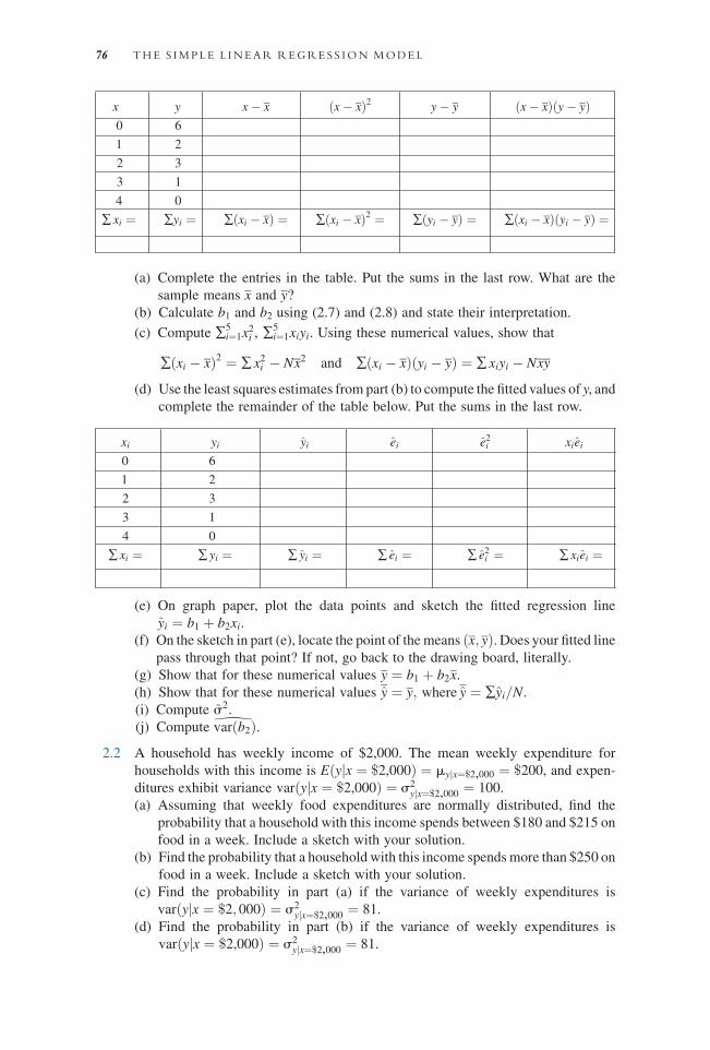
(a) Complete the entries in the table. Put the sums in the last row. What are the

sample means x and y?

(b) Calculate b1 and b2 using (2.7) and (2.8) and state their interpretation.

(c) Compute �5i¼1x

2i , �

5i¼1xiyi. Using these numerical values, show that

�ðxi � xÞ2 ¼ � x2i � Nx2 and �ðxi � xÞðyi � yÞ ¼ � xiyi � Nxy

(d) Use the least squares estimates from part (b) to compute the fitted values of y, and

complete the remainder of the table below. Put the sums in the last row.

(e) On graph paper, plot the data points and sketch the fitted regression line

yi ¼ b1 þ b2xi.

(f) On the sketch in part (e), locate the point of the means ðx; yÞ. Does your fitted linepass through that point? If not, go back to the drawing board, literally.

(g) Show that for these numerical values y ¼ b1 þ b2x.

(h) Show that for these numerical values y ¼ y; where y ¼ �yi=N.(i) Compute s2.

(j) Computebvarðb2Þ.2.2 A household has weekly income of $2,000. The mean weekly expenditure for

households with this income is Eðyjx ¼ $2,000Þ ¼ myjx¼$2,000 ¼ $200, and expen-

ditures exhibit variance varðyjx ¼ $2,000Þ ¼ s2yjx¼$2,000 ¼ 100.

(a) Assuming that weekly food expenditures are normally distributed, find the

probability that a household with this income spends between $180 and $215 on

food in a week. Include a sketch with your solution.

(b) Find the probability that a household with this income spends more than $250 on

food in a week. Include a sketch with your solution.

(c) Find the probability in part (a) if the variance of weekly expenditures is

varðyjx ¼ $2; 000Þ ¼ s2yjx¼$2,000 ¼ 81.

(d) Find the probability in part (b) if the variance of weekly expenditures is

varðyjx ¼ $2,000Þ ¼ s2yjx¼$2,000 ¼ 81.

x y x� x ðx� xÞ2 y� y ðx� xÞðy� yÞ0 6

1 2

2 3

3 1

4 0

� xi ¼ �yi ¼ �ðxi � xÞ ¼ �ðxi � xÞ2 ¼ �ðyi � yÞ ¼ �ðxi � xÞðyi � yÞ ¼

xi yi yi ei e2i xiei

0 6

1 2

2 3

3 1

4 0

� xi ¼ � yi ¼ � yi ¼ � ei ¼ � e2i ¼ � xiei ¼

76 THE S IMPLE L INEAR REGRESS ION MODEL

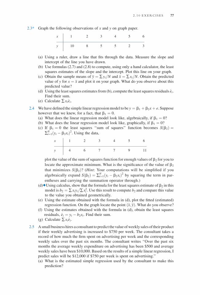
2.3* Graph the following observations of x and y on graph paper.

(a) Using a ruler, draw a line that fits through the data. Measure the slope and

intercept of the line you have drawn.

(b) Use formulas (2.7) and (2.8) to compute, using only a hand calculator, the least

squares estimates of the slope and the intercept. Plot this line on your graph.

(c) Obtain the sample means of y ¼ � yi=N and x ¼ � xi=N. Obtain the predicted

value of y for x ¼ x and plot it on your graph. What do you observe about this

predicted value?

(d) Using the least squares estimates from (b), compute the least squares residuals ei.

Find their sum.

(e) Calculate � xiei.

2.4 We have defined the simple linear regressionmodel to be y ¼ b1 þ b2xþ e. Suppose

however that we knew, for a fact, that b1 ¼ 0.

(a) What does the linear regression model look like, algebraically, if b1 ¼ 0?

(b) What does the linear regression model look like, graphically, if b1 ¼ 0?

(c) If b1 ¼ 0 the least squares ‘‘sum of squares’’ function becomes Sðb2Þ ¼�N

i¼1ðyi � b2xiÞ2. Using the data,

plot the value of the sum of squares function for enough values of b2 for you to

locate the approximate minimum. What is the significance of the value of b2

that minimizes Sðb2Þ? (Hint: Your computations will be simplified if you

algebraically expand Sðb2Þ ¼ �Ni¼1ðyi � b2xiÞ2 by squaring the term in par-

entheses and carrying the summation operator through.)

(d)^Using calculus, show that the formula for the least squares estimate of b2 in this

model is b2 ¼ � xiyi=� x2i . Use this result to compute b2 and compare this value

to the value you obtained geometrically.

(e) Using the estimate obtained with the formula in (d), plot the fitted (estimated)

regression function. On the graph locate the point ðx; yÞ. What do you observe?

(f) Using the estimates obtained with the formula in (d), obtain the least squares

residuals, ei ¼ yi � b2xi. Find their sum.

(g) Calculate � xiei.

2.5 Asmall business hires a consultant to predict thevalue ofweekly sales of their product

if their weekly advertising is increased to $750 per week. The consultant takes a

record of how much the firm spent on advertising per week and the corresponding

weekly sales over the past six months. The consultant writes ‘‘Over the past six

months the average weekly expenditure on advertising has been $500 and average

weekly sales have been $10,000. Based on the results of a simple linear regression, I

predict sales will be $12,000 if $750 per week is spent on advertising.’’

(a) What is the estimated simple regression used by the consultant to make this

prediction?

x 1 2 3 4 5 6

y 10 8 5 5 2 3

x 1 2 3 4 5 6

y 4 6 7 7 9 11

2 . 1 0 EXERCI SE S 77

(b) Sketch a graph of the estimated regression line. Locate the averageweekly values

on the graph.

2.6* A soda vendor at Louisiana State University football games observes that more sodas

are sold the warmer the temperature at game time is. Based on 32 home games

covering five years, the vendor estimates the relationship between soda sales and

temperature to be y ¼ �240þ 8x, where y ¼ the number of sodas she sells and x ¼temperature in degrees Fahrenheit,

(a) Interpret the estimated slope and intercept. Do the estimates make sense? Why,

or why not?

(b) On a day when the temperature at game time is forecast to be 808F, predict howmany sodas the vendor will sell.

(c) Below what temperature are the predicted sales zero?

(d) Sketch a graph of the estimated regression line.

2.7 You have the results of a simple linear regression based on state-level data and the

District of Columbia, a total of N ¼ 51 observations.

(a) The estimated error variance s2 ¼ 2:04672.What is the sum of the squared least

squares residuals?

(b) The estimated variance of b2 is 0.00098. What is the standard error of b2? What

is the value of �ðxi � xÞ2?(c) Suppose the dependent variable yi ¼ the state’s mean income (in thousands of

dollars) of males who are 18 years of age or older and xi the percentage of males

18 years or older who are high school graduates. If b2 ¼ 0:18, interpret thisresult.

(d) Suppose x ¼ 69:139 and y ¼ 15:187, what is the estimate of the intercept

parameter?

(e) Given the results in (b) and (d), what is � x2i ?(f) For the state of Arkansas the value of yi ¼ 12:274 and the value of xi ¼ 58:3:

Compute the least squares residual for Arkansas. (Hint: Use the information in

parts (c) and (d).).

2.8^ Professor E.Z. Stuff has decided that the least squares estimator is too much trouble.

Noting that two points determine a line, Dr. Stuff chooses two points from a sample of

size N and draws a line between them, calling the slope of this line the EZ estimator

of b2 in the simple regression model. Algebraically, if the two points are ðx1; y1Þand ðx2; y2Þ, the EZ estimation rule is

bEZ ¼ y2 � y1

x2 � x1

Assuming that all the assumptions of the simple regression model hold:

(a) Show that bEZ is a ‘‘linear’’ estimator.

(b) Show that bEZ is an unbiased estimator.

(c) Find the variance of bEZ.

(d) Find the probability distribution of bEZ.

(e) Convince Professor Stuff that the EZ estimator is not as good as the least squares

estimator. No proof is required here.

2.10.2 COMPUTER EXERCISES

2.9* The owners of a motel discovered that a defective product was used in its construc-

tion. It took seven months to correct the defects, during which 14 rooms in the

78 THE S IMPLE L INEAR REGRESS ION MODEL

100-unit motel were taken out of service for 1 month at a time. The motel lost

profits due to these closures, and the question of how to compute the losses was

addressed by Adams (2008).7 For this exercise use the data in motel.dat.

(a) The occupancy rate for the damaged motel isMOTEL_PCT, and the competitor

occupancy rate is COMP_PCT. On the same graph, plot these variables against

TIME. Which had the higher occupancy before the repair period?Which had the

higher occupancy during the repair period?

(b) Plot MOTEL_PCT against COMP_PCT. Does there seem to be a relationship

between these two variables? Explain why such a relationship might exist.

(c) Estimate a linear regression with y ¼ MOTEL_PCT and x ¼ COMP_PCT.

Discuss the result.

(d) Compute the least squares residuals from the regression results in (c). Plot these

residuals against time. Does the model overpredict, underpredict, or accurately

predict the motel’s occupancy rate during the repair period?

(e) Consider a linear regressionwith y¼MOTEL_PCTand x¼RELPRICE, which is

the ratio of the price per room charged by the motel in question relative to its

competitors. What sign do you predict for the slope coefficient? Why? Does the

sign of the estimated slope agree with your expectation?

(f) Consider the linear regression with y¼MOTEL_PCTand x¼ REPAIR, which is

an indicator variable, taking the value 1 during the repair period and 0 otherwise.

Discuss the interpretation of the least squares estimates. Does themotel appear to

have suffered a loss of occupancy, and therefore profits, during the repair period?

(g) Compute the average occupancy rate for the motel and competitors when the

repairs were not being made (call these MOTEL0 and COMP0), and when they

were being made (MOTEL1 and COMP1). During the nonrepair period, what

was the difference between the average occupancies,MOTEL0 � COMP0?Does

this comparison seem to support the motel’s claims of lost profits during the

repair period?

(h) Estimate a linear regressionmodel with y¼MOTEL_PCT–COMP_PCTand x¼REPAIR. How do the results of this regression relate to the result in part (g)?

2.10 The capital asset pricingmodel (CAPM) is an important model in the field of finance.

It explains variations in the rate of return on a security as a function of the rate of

return on a portfolio consisting of all publicly traded stocks, which is called the

market portfolio. Generally the rate of return on any investment is measured relative

to its opportunity cost, which is the return on a risk free asset. The resulting difference

is called the risk premium, since it is the reward or punishment for making a risky

investment. The CAPM says that the risk premium on security j is proportional to the

risk premium on the market portfolio. That is,

rj � rf ¼ bjðrm � rf Þ,where rj and rf are the returns to security j and the risk-free rate, respectively, rm is

the return on the market portfolio, and bj is the jth security’s ‘‘beta’’ value. A stock’s

beta is important to investors since it reveals the stock’s volatility. It measures the

sensitivity of security j’s return to variation in the whole stock market. As such,

values of beta less than 1 indicate that the stock is ‘‘defensive’’ since its variation is

7 A. Frank Adams (2008) ‘‘When a ‘Simple’ Analysis Won’t Do: Applying Economic Principles in a Lost

Profits Case,’’ The Value Examiner, May/June 2008, 22–28. The authors thank Professor Adams for the use of

his data.

2 . 1 0 EXERCI SE S 79

less than the market’s. A beta greater than 1 indicates an ‘‘aggressive stock.’’

Investors usually want an estimate of a stock’s beta before purchasing it. The CAPM

model shown above is the ‘‘economic model’’ in this case. The ‘‘econometric

model’’ is obtained by including an intercept in themodel (even though theory says it

should be zero) and an error term,

rj � rf ¼ aj þ bjðrm � rf Þ þ e

(a) Explain why the econometric model above is a simple regression model like

those discussed in this chapter.

(b) In the data file capm4.dat are data on themonthly returns of six firms (Microsoft,

GE, GM, IBM, Disney, and Mobil-Exxon), the rate of return on the market

portfolio (MKT ), and the rate of return on the risk free asset (RISKFREE). The

132 observations cover January 1998 to December 2008. Estimate the CAPM

model for each firm, and comment on their estimated beta values. Which firm

appears most aggressive? Which firm appears most defensive?

(c) Finance theory says that the intercept parameter aj should be zero. Does this

seem correct given your estimates? For the Microsoft stock, plot the fitted

regression line along with the data scatter.

(d) Estimate the model for each firm under the assumption that aj ¼ 0. Do the

estimates of the beta values change much?

2.11 The file br2.dat contains data on 1080 houses sold in Baton Rouge, Louisiana, during

mid-2005. The data include sale price, the house size in square feet, its age, whether it

has a pool or fireplace or is on the waterfront. Also included is an indicator variable

TRADITIONAL indicating whether the house style is traditional or not.8 Variable

descriptions are in the file br2.def.

(a) Plot house price against house size for houses with traditional style.

(b) For the traditional-style houses estimate the linear regression model PRICE ¼b1 þ b2SQFT þ e. Interpret the estimates. Draw a sketch of the fitted line.

(c) For the traditional-style houses estimate the quadratic regression model

PRICE ¼ a1 þ a2SQFT2 þ e. Compute the marginal effect of an additional

square foot of living area in a home with 2000 square feet of living space.

Compute the elasticity of PRICE with respect to SQFT for a home with 2000

square feet of living space. Graph the fitted line. On the graph, sketch the line that

is tangent to the curve for a 2000-square-foot house.

(d) For the regressions in (b) and (c) compute the least squares residuals and plot

them against SQFT. Do any of our assumptions appear violated?

(e) One basis for choosing between these two specifications is how well the data are

fit by the model. Compare the sum of squared residuals (SSE) from the models in

(b) and (c).Whichmodel has a lower SSE?Howdoes having a lower SSE indicate

a ‘‘better-fitting’’ model?

(f) For the traditional-style houses estimate the log-linear regression model

lnðPRICEÞ ¼ g1 þ g2SQFT þ e. Interpret the estimates. Graph the fitted line,

and sketch the tangent line to the curve for a house with 2000 square feet of

living area.

8 The data file br.datoffers awider range of style listings. Try this data set for amore detailed investigation of the

effect of style.

80 THE S IMPLE L INEAR REGRESS ION MODEL

(g) How would you compute the sum of squared residuals for the model in (f ) to

make it comparable to those from themodels in (b) and (c)? Compare this sum of

squared residuals to the SSE from the linear and quadratic specifications. Which

model seems to fit the data best?

2.12* The file stockton4.dat contains data on 15009 houses sold in Stockton, CA during

1996–1998. Variable descriptions are in the file stockton4.def.

(a) Plot house selling price against house living area for all houses in the sample.

(b) Estimate the regression model SPRICE ¼ b1 þ b2LIVAREA þ e for all the

houses in the sample. Interpret the estimates. Draw a sketch of the fitted line.

(c) Estimate the quadratic model SPRICE ¼ a1 þ a2LIVAREA2 þ e for all the

houses in the sample. What is the marginal effect of an additional 100 square

feet of living area for a home with 1500 square feet of living area?

(d) In the same graph, plot the fitted lines from the linear and quadratic models.

Which seems to fit the data better? Compare the sum of squared residuals (SSE)

for the two models. Which is smaller?

(e) Estimate the regression model in (c) using only houses that are on large lots.

Repeat the estimation for houses that are not on large lots. Interpret the estimates.

How do the estimates compare?

(f) Plot house selling price against AGE. Estimate the linear model SPRICE ¼d1 þ d2AGE þ e. Interpret the estimated coefficients. Repeat this exercise using

the log-linear model lnðSPRICEÞ ¼ u1 þ u2AGE þ e. Based on the plots and

visual fit of the estimated regression lines, which of these twomodels would you

prefer? Explain.

(g) Estimate a linear regression SPRICE ¼ h1 þ h2LGELOT þ e with dependent

variable SPRICE and independent variable the indicator LGELOTwhich ident-

ifies houses on larger lots. Interpret these results.

2.13 A longitudinal experiment was conducted in Tennessee beginning in 1985 and

ending in 1989. A single cohort of students was followed from kindergarten through

third grade. In the experiment children were randomly assigned within schools into

three types of classes: small classes with 13–17 students, regular-sized classes with

22–25 students, and regular-sized classes with a full-time teacher aide to assist the

teacher. Student scores on achievement tests were recorded as well as some

information about the students, teachers, and schools. Data for the kindergarten

classes are contained in the data file star.dat.

(a) Using children who are in either a regular-sized class or a small class, estimate

the regressionmodel explaining students’ combined aptitude scores as a function

of class size, TOTALSCOREi ¼ b1 þ b2SMALLi þ ei. Interpret the estimates.

Based on this regression result, what do you conclude about the effect of class

size on learning?

(b) Repeat part (a) using dependent variables READSCORE andMATHSCORE. Do

you observe any differences?

(c) Using childrenwho are in either a regular-sized class or a regular-sized classwith

a teacher aide, estimate the regression model explaining student’s combined

aptitude scores as a function of the presence of a teacher aide,

TOTALSCORE ¼ g1 þ g2AIDE þ e. Interpret the estimates. Based on this

9 The data set stockton3.dat has 2,610 observations on these same variables.

2 . 1 0 EXERCI SE S 81

regression result, what do you conclude about the effect on learning of adding a

teacher aide to the classroom?

(d) Repeat part (c) using dependent variables READSCORE and MATHSCORE.

Do you observe any differences?

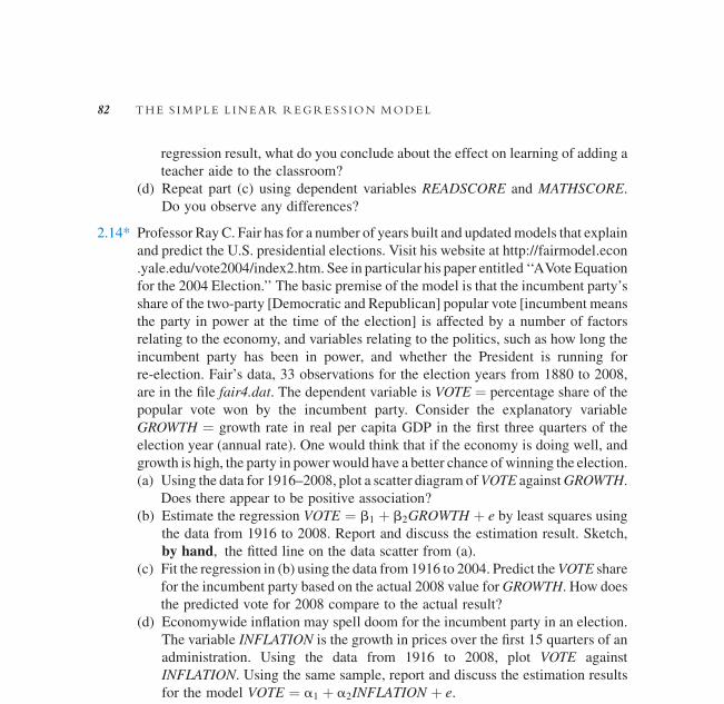
2.14* Professor Ray C. Fair has for a number of years built and updatedmodels that explain

and predict the U.S. presidential elections. Visit his website at http://fairmodel.econ

.yale.edu/vote2004/index2.htm. See in particular his paper entitled ‘‘AVote Equation

for the 2004 Election.’’ The basic premise of the model is that the incumbent party’s

share of the two-party [Democratic and Republican] popular vote [incumbent means

the party in power at the time of the election] is affected by a number of factors

relating to the economy, and variables relating to the politics, such as how long the

incumbent party has been in power, and whether the President is running for

re-election. Fair’s data, 33 observations for the election years from 1880 to 2008,

are in the file fair4.dat. The dependent variable is VOTE ¼ percentage share of the

popular vote won by the incumbent party. Consider the explanatory variable

GROWTH ¼ growth rate in real per capita GDP in the first three quarters of the

election year (annual rate). One would think that if the economy is doing well, and

growth is high, the party in powerwould have a better chance ofwinning the election.

(a) Using the data for 1916–2008, plot a scatter diagram ofVOTE againstGROWTH.

Does there appear to be positive association?

(b) Estimate the regression VOTE ¼ b1 þ b2GROWTH þ e by least squares using

the data from 1916 to 2008. Report and discuss the estimation result. Sketch,

by hand, the fitted line on the data scatter from (a).

(c) Fit the regression in (b) using the data from 1916 to 2004. Predict theVOTE share

for the incumbent party based on the actual 2008 value forGROWTH. How does

the predicted vote for 2008 compare to the actual result?

(d) Economywide inflation may spell doom for the incumbent party in an election.

The variable INFLATION is the growth in prices over the first 15 quarters of an

administration. Using the data from 1916 to 2008, plot VOTE against

INFLATION. Using the same sample, report and discuss the estimation results

for the model VOTE ¼ a1 þ a2INFLATION þ e.

2.15 How much does education affect wage rates? The data file cps4_small.dat contains

1000 observations on hourlywage rates, education, and other variables from the 2008

Current Population Survey (CPS).

(a) Obtain the summary statistics and histograms for the variables WAGE and

EDUC. Discuss the data characteristics.

(b) Estimate the linear regression WAGE ¼ b1 þ b2EDUC þ e and discuss the

results.

(c) Calculate the least squares residuals and plot them against EDUC. Are any

patterns evident? If assumptions SR1–SR5 hold, should any patterns be evident

in the least squares residuals?

(d) Estimate separate regressions for males, females, blacks, and whites. Compare

the results.

(e) Estimate the quadratic regressionWAGE ¼ a1 þ a2EDUC2 þ e and discuss the

results. Estimate the marginal effect of another year of education on wage for a

person with 12 years of education, and for a person with 14 years of education.

Compare these values to the estimated marginal effect of education from the

linear regression in part (b).

82 THE S IMPLE L INEAR REGRESS ION MODEL

The corresponding null hypothesis is the logical alternative to the executive’s statement

H0 : b1 þ b220 � 250; or H1 : b1 þ b220� 250 � 0

Notice that the null and alternative hypothesis are in the same form as the general linear

hypothesis with c1 ¼ 1, c2 ¼ 20, and c0 ¼ 250.

The rejection region for a right-tail test is illustrated in Figure 3.2. For a right-tail test at

the a ¼ 0.05 level of significance the t-critical value is the 95th percentile of the t(38)distribution, which is t(0.95,38)¼ 1.686. If the calculated t-statistic value is greater than 1.686,

wewill reject the null hypothesis and accept the alternative hypothesis, which in this case is

the executive’s conjecture.

Computing the t-statistic value

t ¼ b1 þ 20b2ð Þ � 250

se b1 þ 20b2ð Þ

¼ 83:4160þ 20 10:2096ð Þ � 250

14:1780

¼ 287:6089� 250

14:1780¼ 37:6089

14:1780¼ 2:65

Since t ¼ 2:65 > tc ¼ 1:686, we reject the null hypothesis that a household with weekly

incomeof $2,000will spend $250 perweek or less on food, and conclude that the executive’s

conjecture that such households spend more than $250 is correct, with the probability of

Type I error 0.05.

In Section 3.6.1 we estimated that a household with $2,000 weekly income will spend

$287.6089, which is greater than the executive’s speculated value of $250. However, simply

observing that the estimated value is greater than $250 is not a statistical test. It might be

numerically greater, but is it significantly greater? The t-test takes into account the precision

with which we have estimated this expenditure level and also controls the probability of

Type I error.

3.7 Exercises

Answers to exercises marked * appear at www.wiley.com/college/hill.

3.7.1 PROBLEMS

3.1 Using the regression output for the food expenditure model shown in Figure 2.9:

(a) Construct a 95% interval estimate for b1 and interpret.

(b) Test the null hypothesis that b1 is zero against the alternative that it is not at the

5% level of significance without using the reported p-value. What is your

conclusion?

(c) Draw a sketch showing the p-value 0.0622 shown in Figure 2.9, the critical

value from the t-distribution used in (b), and how the p-value could have been

used to answer (b).

(d) Test the null hypothesis that b1 is zero against the alternative that it is positive

at the 5% level of significance. Drawa sketch of the rejection region and compute

the p-value. What is your conclusion?

118 INTERVAL EST IMAT ION AND HYPOTHES I S TEST ING

(e) Explain the differences and similarities between the ‘‘level of significance’’ and

the ‘‘level of confidence.’’

(f) The results in (d) show that we are 95% confident that b1 is positive. True, or

false? If false, explain.

3.2 The general manager of an engineering firmwants to knowwhether a technical artist’s

experience influences the quality of his or her work. A random sample of 24 artists

is selected and their years of work experience and quality rating (as assessed by

their supervisors) recorded. Work experience (EXPER) is measured in years and

quality rating (RATING) takes a value of 1 through 7, with 7 ¼ excellent and 1 ¼poor: The simple regression model RATING ¼ b1 þ b2EXPERþ e is proposed.

The least squares estimates of the model, and the standard errors of the estimates, are

bRATING ¼ 3:204 þ 0:076EXPERðseÞ ð0:709Þ ð0:044Þ

(a) Sketch the estimated regression function. Interpret the coefficient of EXPER.

(b) Construct a 95% confidence interval forb2, the slope of the relationship between

quality rating and experience. In what are you 95% confident?

(c) Test the null hypothesis that b2 is zero against the alternative that it is not using a

two-tail test and the a ¼ 0:05 level of significance. What do you conclude?

(d) Test the null hypothesis that b2 is zero against the one-tail alternative that it is

positive at the a ¼ 0:05 level of significance. What do you conclude?

(e) For the test in part (c), the p-value is 0.0982. If we choose the probability of a

Type I error to bea ¼ 0:05; dowe reject the null hypothesis, or not, just based onan inspection of the p-value? Show, in a diagram, how this p-value is computed.

3.3* In an estimated simple regression model, based on 24 observations, the estimated

slope parameter is 0.310 and the estimated standard error is 0.082.

(a) Test the hypothesis that the slope is zero against the alternative that it is not, at the

1% level of significance.

(b) Test the hypothesis that the slope is zero against the alternative that it is positive

at the 1% level of significance.

(c) Test the hypothesis that the slope is zero against the alternative that it is negative

at the 5% level of significance. Draw a sketch showing the rejection region.

(d) Test the hypothesis that the estimated slope is 0.5, against the alternative that it is

not, at the 5% level of significance.

(e) Obtain a 99% interval estimate of the slope.

3.4 Consider a simple regression in which the dependent variableMIM ¼mean income

of males who are 18 years of age or older, in thousands of dollars. The explanatory

variable PMHS ¼ percent of males 18 or older who are high school graduates. The

data consist of 51 observations on the 50 states plus the District of Columbia. Thus

MIM andPMHS are ‘‘state averages.’’ The estimated regression, along with standard

errors and t-statistics, is

bMIM ¼ ðaÞ þ 0:180PMHS

ðseÞ ð2:174Þ ðbÞðtÞ ð1:257Þ ð5:754Þ

(a) What is the estimated equation intercept? Show your calculation. Sketch the

estimated regression function.

3 . 7 EXERCI SES 119

(b) What is the standard error of the estimated slope? Show your calculation.

(c) What is the p-value for the two-tail test of the hypothesis that the equation

intercept is zero? Draw a sketch to illustrate.

(d) State the economic interpretation of the estimated slope. Is the sign of the

coefficient what you would expect from economic theory?

(e) Construct a 99% confidence interval estimate of the slope of this relationship.

(f) Test the hypothesis that the slope of the relationship is 0.2 against the alternative

that it is not. State in words the meaning of the null hypothesis in the context of

this problem.

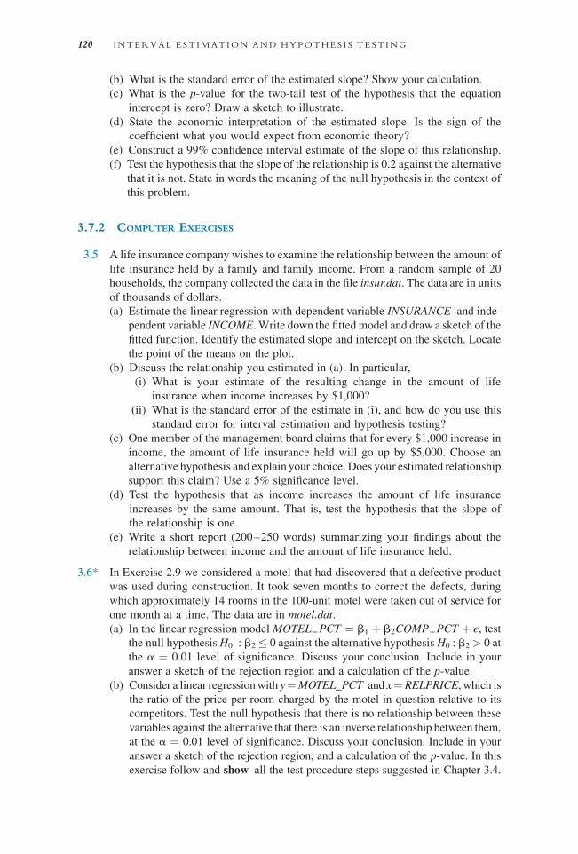
3.7.2 COMPUTER EXERCISES

3.5 A life insurance company wishes to examine the relationship between the amount of

life insurance held by a family and family income. From a random sample of 20

households, the company collected the data in the file insur.dat. The data are in units

of thousands of dollars.

(a) Estimate the linear regression with dependent variable INSURANCE and inde-

pendent variable INCOME. Write down the fitted model and draw a sketch of the

fitted function. Identify the estimated slope and intercept on the sketch. Locate

the point of the means on the plot.

(b) Discuss the relationship you estimated in (a). In particular,

(i) What is your estimate of the resulting change in the amount of life

insurance when income increases by $1,000?

(ii) What is the standard error of the estimate in (i), and how do you use this

standard error for interval estimation and hypothesis testing?

(c) One member of the management board claims that for every $1,000 increase in

income, the amount of life insurance held will go up by $5,000. Choose an

alternative hypothesis and explain your choice. Does your estimated relationship

support this claim? Use a 5% significance level.

(d) Test the hypothesis that as income increases the amount of life insurance

increases by the same amount. That is, test the hypothesis that the slope of

the relationship is one.

(e) Write a short report (200–250 words) summarizing your findings about the

relationship between income and the amount of life insurance held.

3.6* In Exercise 2.9 we considered a motel that had discovered that a defective product

was used during construction. It took seven months to correct the defects, during

which approximately 14 rooms in the 100-unit motel were taken out of service for

one month at a time. The data are in motel.dat.

(a) In the linear regression model MOTEL PCT ¼ b1 þ b2COMP PCT þ e, test

the null hypothesis H0 : b2 � 0 against the alternative hypothesis H0 : b2 > 0 at

the a ¼ 0.01 level of significance. Discuss your conclusion. Include in your

answer a sketch of the rejection region and a calculation of the p-value.

(b) Consider a linear regressionwith y¼MOTEL_PCT and x¼RELPRICE, which is

the ratio of the price per room charged by the motel in question relative to its

competitors. Test the null hypothesis that there is no relationship between these

variables against the alternative that there is an inverse relationship between them,

at the a ¼ 0.01 level of significance. Discuss your conclusion. Include in your

answer a sketch of the rejection region, and a calculation of the p-value. In this

exercise follow and show all the test procedure steps suggested in Chapter 3.4.

120 INTERVAL EST IMAT ION AND HYPOTHES I S TEST ING

(c) Consider the linear regression MOTEL PCT ¼ d1 þ d2REPAIR þ e, where

REPAIR is an indicator variable taking the value 1 during the repair period

and 0 otherwise. Test the null hypothesis H0 : d2 � 0 against the alternative

hypothesis H1 : d2 < 0 at the a ¼ 0.05 level of significance. Explain the logic

behind stating the null and alternative hypotheses in this way. Discuss your

conclusions.

(d) Using the model given in part (c), construct a 95% interval estimate for the

parameter d2 and give its interpretation. Have we estimated the effect of the

repairs on motel occupancy relatively precisely, or not? Explain.

(e) Consider the linear regressionmodel with y¼MOTEL_PCT�COMP_PCT and

x ¼ REPAIR, that is MOTEL PCT � COMP PCTð Þ ¼ g1 þ g2REPAIRþ e.

Test the null hypothesis that g2 ¼ 0 against the alternative that g2 < 0 at the a¼0.01 level of significance. Discuss the meaning of the test outcome.

(f) Using themodel in part (e), construct and discuss the 95% interval estimate of g2.

3.7 Consider the capital asset pricing model (CAPM) in Exercise 2.10. Use the data in

capm4.dat to answer each of the following:

(a) Test at the 5% level of significance the hypothesis that each stock’s ‘‘beta’’ value

is 1 against the alternative that it is not equal to 1. What is the economic

interpretation of a beta equal to 1?

(b) Test at the 5% level of significance the null hypothesis that Mobil-Exxon’s

‘‘beta’’ value is greater than or equal to 1 against the alternative that it is less than

1. What is the economic interpretation of a beta less than 1?

(c) Test at the 5% level of significance the null hypothesis that Microsoft’s ‘‘beta’’

value is less than or equal to 1 against the alternative that it is greater than 1.What

is the economic interpretation of a beta more than 1?

(d) Construct a 95% interval estimate ofMicrosoft’s ‘‘beta.’’ Assume that you are a

stockbroker. Explain this result to an investor who has come to you for advice.

(e) Test (at a 5% significance level) the hypothesis that the intercept term in the

CAPMmodel for each stock is zero, against the alternative that it is not.What do

you conclude?

3.8 The file br2.dat contains data on 1080 houses sold in Baton Rouge, Louisiana during

mid-2005. The data include sale price and the house size in square feet. Also included

is an indicator variable TRADITIONAL indicating whether the house style is

traditional or not.

(a) For the traditional-style houses estimate the linear regression model

PRICE ¼ b1 þ b2SQFT þ e. Test the null hypothesis that the slope is zero

against the alternative that it is positive, using the a¼ 0.01 level of significance.

Follow and show all the test steps described in Chapter 3.4.

(b) Using the linearmodel in (a), test the null hypothesis (H0) that the expected price

of a house of 2000 square feet is equal to, or less than, $120,000. What is the

appropriate alternative hypothesis?Use thea¼0.01 level of significance.Obtain

the p-value of the test and show its value on a sketch. What is your conclusion?

(c) Based on the estimated results from part (a), construct a 95% interval estimate of

the expected price of a house of 2000 square feet.

(d) For the traditional-style houses, estimate the quadratic regression model

PRICE ¼ a1 þ a2SQFT2 þ e. Test the null hypothesis that the marginal effect

of an additional square foot of living area in a home with 2000 square feet of

living space is $75 against the alternative that the effect is less than $75. Use the

3 . 7 EXERCI SES 121

a ¼ 0.01 level of significance. Repeat the same test for a home of 4000 square

feet of living space. Discuss your conclusions.

(e) For the traditional-style houses, estimate the log-linear regression model

ln PRICEð Þ ¼ g1 þ g2SQFT þ e. Test the null hypothesis that the marginal

effect of an additional square foot of living area in a home with 2000 square

feet of living space is $75 against the alternative that the effect is less than $75.

Use the a ¼ 0.01 level of significance. Repeat the same test for a home of 4000

square feet of living space. Discuss your conclusions.

3.9* Reconsider the presidential voting data (fair4.dat) introduced in Exercise 2.14. Use

the data from 1916 to 2008 for this exercise.

(a) Using the regression model VOTE ¼ b1 þ b2GROWTH þ e, test (at a 5%

significance level) the null hypothesis that economic growth has no effect on

the percentage vote earned by the incumbent party. Select an alternative

hypothesis and a rejection region. Explain your choice.

(b) Using the regression model in part (a), construct a 95% interval estimate for b2,

and interpret.

(c) Using the regression model VOTE ¼ b1 þ b2INFLATION þ e, test the null

hypothesis that inflation has no effect on the percentage vote earned by the

incumbent party. Select an alternative hypothesis, a rejection region, and a

significance level. Explain your choice.

(d) Using the regression model in part (c), construct a 95% interval estimate for b2,

and interpret.

(e) Test the null hypothesis that if INFLATION ¼ 0 the expected vote in favor of the

incumbent party is 50%, or more. Select the appropriate alternative. Carry out

the test at the 5% level of significance. Discuss your conclusion.

(f) Construct a 95% interval estimate of the expected vote in favor of the incumbent

party if INFLATION ¼ 2%. Discuss the interpretation of this interval estimate.

3.10 Reconsider Exercise 2.13, which was based on the experiment with small classes for

primary school students conducted in Tennessee beginning in 1985. Data for the

kindergarten classes is contained in the data file star.dat.

(a) Using children who are in either a regular-sized class or a small class, estimate

the regressionmodel explaining students’ combined aptitude scores as a function

of class size, TOTALSCORE ¼ b1 þ b2SMALL þ e. Test the null hypothesis

that b2 is zero, or negative, against the alternative that this coefficient is positive.

Use the 5% level of significance. Compute the p-value of this test, and show its

value in a sketch. Discuss the social importance of this finding.

(b) For the model in part (a), construct a 95% interval estimate of b2 and discuss.

(c) Repeat part (a) using dependent variablesREADSCORE andMATHSCORE. Do

you observe any differences?

(d) Using childrenwho are in either a regular-sized class or a regular-sized classwith

a teacher aide, estimate the regression model explaining students’ combined

aptitude scores as a function of the presence or absence of a teacher aide,

TOTALSCORE ¼ g1 þ g2AIDE þ e. Test the null hypothesis that g2 is zero or

negative against the alternative that this coefficient is positive. Use the 5% level

of significance. Discuss the importance of this finding.

(e) For the model in part (d), construct a 95% interval estimate of g2 and discuss.

(f) Repeat part (d) using dependent variables READSCORE and MATHSCORE.

Do you observe any differences?

122 INTERVAL EST IMAT ION AND HYPOTHES I S TEST ING

3.11 Howmuch does experience affect wage rates? The data file cps4_small.dat contains

1000 observations on hourly wage rates, experience and other variables from the

2008 Current Population Survey (CPS).

(a) Estimate the linear regression WAGE ¼ b1 þ b2EXPERþ e and discuss the

results. Using your software plot a scatter diagram with WAGE on the vertical

axis and EXPER on the horizontal axis. Sketch in by hand, or using your

software, the fitted regression line.

(b) Test the statistical significance of the estimated slope of the relationship at the

5% level. Use a one-tail test.

(c) Repeat part (a) for the sub-samples consisting of (i) females, (ii) males, (iii)

blacks, and (iv) white males. What differences, if any, do you notice?

(d) For each of the estimated regression models in (a) and (c), calculate the least

squares residuals and plot them against EXPER. Are any patterns evident?

3.12 Is the relationship between experience and wages constant over one’s lifetime? To

investigate we will fit a quadratic model using the data file cps4_small.dat, which

contains 1,000 observations on hourly wage rates, experience and other variables

from the 2008 Current Population Survey (CPS).

(a) Create a new variable called EXPER30 ¼ EXPER � 30. Construct a scatter

diagram with WAGE on the vertical axis and EXPER30 on the horizontal axis.

Are any patterns evident?

(b) Estimate by least squares the quadraticmodelWAGE ¼ g1 þ g2 EXPER30ð Þ2 þ e.

Are the coefficient estimates statistically significant? Test the null hypothesis that

g2� 0 against the alternative that g2< 0 at thea¼ 0.05 level of significance.What

conclusion do you draw?

(c) Using the estimation in part (b), compute the estimated marginal effect of

experience upon wage for a person with 10 years’ experience, 30 years’

experience, and 50 years’ experience. Are these slopes significantly different

from zero at the a ¼ 0.05 level of significance?

(d) Construct 95% interval estimates of each of the slopes in part (c). How precisely

are we estimating these values?

(e) Using the estimation result from part (b) create the fitted valuesbWAGE ¼ g1 þ g2 EXPER30ð Þ2, where the ^ denotes least squares estimates.

Plot these fitted values andWAGE on the vertical axis of the same graph against

EXPER30 on the horizontal axis. Are the estimates in part (c) consistent with the

graph?

(f) Estimate the linear regression WAGE ¼ b1 þ b2EXPER30þ e and the linear

regression WAGE ¼ a1 þ a2EXPERþ e. What differences do you observe

between these regressions and why do they occur? What is the estimated

marginal effect of experience on wage from these regressions? Based on your

work in parts (b)–(d), is the assumption of constant slope in this model a good

one? Explain.

(g) Use the larger data cps4.dat (4838 observations) to repeat parts (b), (c), and (d).

Howmuch has the larger sample improved the precision of the interval estimates

in part (d)?

3.13* Is the relationship between experience and ln(wages) constant over one’s lifetime?

To investigate wewill fit a log-linear model using the data file cps4_small.dat, which

contains 1000 observations on hourly wage rates, experience and other variables

from the 2008 Current Population Survey (CPS).

3 . 7 EXERCI SES 123

(a) Create a new variable called EXPER30 ¼ EXPER � 30. Construct a scatter

diagramwith ln(WAGE) on thevertical axis andEXPER30 on the horizontal axis.

Are any patterns evident?

(b) Estimate by least squares the quadratic model ln WAGEð Þ ¼ g1þg2 EXPER30ð Þ2 þ e. Are the coefficient estimates statistically significant?

Test the null hypothesis that g2 � 0 against the alternative that g2 < 0 at the

a ¼ 0.05 level of significance. What conclusion do you draw?

(c) Using the estimation in part (b), compute the estimated marginal effect

of experience upon wage for a person with 10 years of experience, 30 years of

experience, and 50 years of experience. [Hint: If ln yð Þ ¼ aþ bx2 then

y ¼ exp aþ bx2ð Þ, and dy=dx ¼ exp aþ bx2ð Þ 2bx ¼ 2bxy]

(d) Using the estimation result from part (b) create the fitted valuesbWAGE ¼ exp g1 þ g2 EXPER30ð Þ2� �

, where the ^ denotes least squares esti-

mates. Plot these fitted values and WAGE on the vertical axis of the same graph

against EXPER30 on the horizontal axis. Are the estimates in part (c) consistent

with the graph?

3.14 Data on theweekly sales of a major brand of canned tuna by a supermarket chain in a

largemidwestern U.S. city during amid-1990s calendar year are contained in the file

tuna.dat. There are 52 observations on the variables. The variable SAL1¼ unit sales

of brand no. 1 canned tuna, APR1¼ price per can of brand no. 1 canned tuna, APR2,

APR3 ¼ price per can of brands nos. 2 and 3 of canned tuna.

(a) Create the relative price variables RPRICE2 ¼ APR1/APR2 and RPRICE3 ¼APR1/APR3. What do you anticipate the relationship between sales (SAL1) and

the relative price variables to be? Explain your reasoning.

(b) Estimate the log-linear model ln SAL1ð Þ ¼ b1 þ b2RPRICE2þ e. Interpret the

estimate of b2. Construct and interpret a 95% interval estimate of the parameter.

(c) Test the null hypothesis that the slope of the relationship in (b) is zero. Create the

alternative hypothesis based on your answer to part (a). Use the 1% level of

significance and draw a sketch of the rejection region. Is your result consistent

with economic theory?

(d) Estimate the log-linear model ln SAL1ð Þ ¼ g1 þ g2RPRICE3þ e. Interpret the

estimate of g2. Construct and interpret a 95% interval estimate of the parameter.

(e) Test the null hypothesis that the slope of this relationship is zero. Create the

alternative hypothesis based on your answer to part (a). Use the 1% level of

significance and draw a sketch of the rejection region. Is your result consistent

with economic theory?

3.15 What is the relationship between crime and punishment? This important question has

been examined by Cornwell and Trumbull2 using a panel of data from North

Carolina. The cross sections are 90 counties, and the data are annual for the years

1981–1987. The data are in the file crime.dat.

(a) Using the data from 1987, estimate the log-linear regression relating the log of the

crime rate to the probability of an arrest, LCRMRTE ¼ b1 þ b2PRBARRþ e.

The probability of arrest is measured as the ratio of arrests to offenses. If

we increase the probability of arrest by 10%, what will be the effect on the crime

rate? What is a 95% interval estimate of this quantity?

2 ‘‘Estimating the Economic Model of Crimewith Panel Data,’’ Review of Economics and Statistics, 76, 1994,

360–366. The data were kindly provided by the authors.

124 INTERVAL EST IMAT ION AND HYPOTHES I S TEST ING

(b) Test the null hypothesis that there is no relationship between the crime rate and

the probability of arrest against the alternative that there is an inverse relation-

ship. Use the 1% level of significance.

(c) Repeat parts (a) and (b) using the probability of conviction (PRBCONV) as the

explanatory variable. The probability of conviction is measured as the ratio of

convictions to arrests.

Appendix 3A Derivation of the t-Distribution

Interval estimation and hypothesis testing procedures in this chapter involve the t-distribution.

Here we develop the key result.

The first result that is needed is the normal distribution of the least squares estimator.

Consider, for example, the normal distribution of b2 the least squares estimator ofb2, which

we denote as

b2 �N b2;s2

�ðxi � xÞ2 !

A standardized normal random variable is obtained from b2 by subtracting its mean and

dividing by its standard deviation:

Z ¼ b2 � b2ffiffiffiffiffiffiffiffiffiffiffiffiffiffiffivarðb2Þ

p �Nð0; 1Þ (3A.1)

That is, the standardized random variable Z is normally distributed with mean 0 and

variance 1.

The second piece of the puzzle involves a chi-square randomvariable. If assumption SR6

holds, then the random error term ei has a normal distribution, ei �Nð0;s2Þ. Again, we canstandardize the randomvariable by dividing by its standard deviation so that ei=s�Nð0; 1Þ.The square of a standard normal random variable is a chi-square random variable (see

Appendix B.5.2) with one degree of freedom, so ðei=sÞ2 � x2ð1Þ. If all the random errors are

independent, then

�ei

s

� �2¼ e1

s

� �2þ e2

s

� �2þ � � � þ eN

s

� �2� x2ðNÞ (3A.2)

Since the true random errors are unobservable, we replace them by their sample counter-

parts, the least squares residuals ei ¼ yi � b1 � b2xi, to obtain

V ¼ �e2is2

¼ ðN � 2Þs2

s2(3A.3)

The random variable V in (3A.3) does not have a x2ðNÞ distribution, because the least squaresresiduals are not independent random variables. All N residuals ei ¼ yi � b1 � b2xi depend

on the least squares estimators b1 and b2. It can be shown that onlyN � 2 of the least squares

residuals are independent in the simple linear regression model. Consequently, the random

variable in (3A.3) has a chi-square distribution with N � 2 degrees of freedom. That is,

when multiplied by the constant ðN � 2Þ=s2, the random variable s2 has a chi-square

distribution with N � 2 degrees of freedom,

APPENDIX 3A DERIVAT ION OF THE t -D I STR IBUT ION 125

The estimated log-log model is

bln Qð Þ ¼ 3:717� 1:121� ln Pð Þ R2g ¼ 0:8817

ðseÞ ð0:022Þ ð0:049Þ (4.15)

We estimate that the price elasticity of demand is 1.121: a 1% increase in real price is

estimated to reduce quantity consumed by 1.121%.

The fitted line shown in Figure 4.16 is the ‘‘corrected’’ predictor discussed in Section

4.5.3. The corrected predictor Qc is the natural predictor Qn adjusted by the factor

exp s2�2

� �. That is, using the estimated error variance s2 ¼ 0:0139, the predictor is

Qc ¼ Qnes2=2 ¼ expbln Qð Þ

� �es

2=2 ¼ exp�3:717� 1:121� ln Pð Þ�e0:0139=2

The goodness-of-fit statisticR2g ¼ 0:8817 is the generalized R2 discussed in Section 4.5.4. It

is the squared correlation between the predictor Qc and the observations Q

R2g ¼ corr Q; Qc

� �� 2 ¼ 0:939½ �2 ¼ 0:8817

4.7 Exercises

Answer to exercises marked * appear www.wiley.com/college/hill.

4.7.1 PROBLEMS

4.1* (a) Supposing that a simple regression has quantities �ðyi � yÞ2 ¼ 631:63 and

�e2i ¼ 182:85, find R2.

(b) Suppose that a simple regression has quantities N ¼ 20, �y2i ¼ 5930:94,y ¼ 16:035, and SSR ¼ 666:72, find R2.

(c) Suppose that a simple regression has quantitiesR2 ¼ 0:7911, SST ¼ 552:36, andN ¼ 20, find s2.

10

20

30

40

50

1 1.5 2

Price of Chicken

Poultry Demand

Qua

ntity

of

Chi

cken

2.5 3

FIGURE 4.16 Quantity and Price of Chicken.

4 . 7 EXERCI SES 157

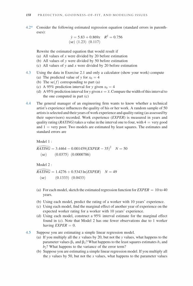
4.2* Consider the following estimated regression equation (standard errors in parenth-

eses):

y ¼ 5:83þ 0:869x R2 ¼ 0:756ðseÞ ð1:23Þ ð0:117Þ

Rewrite the estimated equation that would result if

(a) All values of x were divided by 20 before estimation

(b) All values of y were divided by 50 before estimation

(c) All values of y and x were divided by 20 before estimation

4.3 Using the data in Exercise 2.1 and only a calculator (show your work) compute

(a) The predicted value of y for x0 ¼ 4

(b) The seð f Þ corresponding to part (a)

(c) A 95% prediction interval for y given x0 ¼ 4

(d) A 95%prediction interval for y given x ¼ x. Compare thewidth of this interval to

the one computed in part (c)

4.4 The general manager of an engineering firm wants to know whether a technical

artist’s experience influences the quality of his or her work. A random sample of 50

artists is selected and their years ofwork experience and quality rating (as assessed by

their supervisors) recorded. Work experience (EXPER) is measured in years and

quality rating (RATING) takes a value in the interval one to four, with 4 ¼ very good

and 1 ¼ very poor. Two models are estimated by least squares. The estimates and

standard errors are

Model 1 :bRATING ¼ 3:4464� 0:001459 EXPER� 35ð Þ2 N ¼ 50

ðseÞ ð0:0375Þ ð0:0000786Þ

Model 2 :bRATING ¼ 1:4276þ 0:5343 ln EXPERð Þ N ¼ 49

ðseÞ ð0:1333Þ ð0:0433Þ

(a) For each model, sketch the estimated regression function for EXPER ¼ 10 to 40

years.

(b) Using each model, predict the rating of a worker with 10 years’ experience.

(c) Using each model, find the marginal effect of another year of experience on the

expected worker rating for a worker with 10 years’ experience.

(d) Using each model, construct a 95% interval estimate for the marginal effect

found in (c). Note that Model 2 has one fewer observations due to 1 worker

having EXPER ¼ 0.

4.5 Suppose you are estimating a simple linear regression model.

(a) If you multiply all the x values by 20, but not the y values, what happens to the

parameter values b1 and b2? What happens to the least squares estimates b1 and

b2? What happens to the variance of the error term?

(b) Suppose you are estimating a simple linear regression model. If you multiply all

the y values by 50, but not the x values, what happens to the parameter values

158 PRED ICT ION , GOODNESS -OF - F IT , AND MODEL ING I S SUES

b1 and b2?What happens to the least squares estimates b1 and b2?What happens

to the variance of the error term?

4.6 The fitted least squares line is yi ¼ b1 þ b2xi.

(a) Algebraically, show that the fitted line passes through the point of the means,

ðx; yÞ.(b) Algebraically show that the average value of yi equals the sample average of y.

That is, show that y ¼ y; where y ¼ �yi=N.

4.7 In a simple linear regression model suppose we know that the intercept parameter is

zero, so the model is yi ¼ b2xi þ ei. The least squares estimator of b2 is developed in

Exercise 2.4.

(a) What is the least squares predictor of y in this case?

(b) When an intercept is not present in a model, R2 is often defined to be

R2u ¼ 1� SSE=�y2i , where SSE is the usual sum of squared residuals. Compute

R2u for the data in Exercise 2.4.

(c) Compare the value of R2u in part (b) to the generalized R2 ¼ r2yy, where y is the

predictor based on the restricted model in part (a).

(d) Compute SST ¼ �ðyi � yÞ2 and SSR ¼ �ðyi � yÞ2, where y is the predictor

based on the restricted model in part (a). Does the sum of squares decomposition

SST ¼ SSR þ SSE hold in this case?

4.7.2 COMPUTER EXERCISES

4.8 The first three columns in the filewa_wheat.dat contain observations on wheat yield

in the Western Australian shires Northampton, Chapman Valley, and Mullewa,

respectively. There are 48 annual observations for the years 1950–1997. For the

Chapman Valley shire, consider the three equations

yt ¼ b1 þ b2t þ et

yt ¼ a1 þ a2lnðtÞ þ et

yt ¼ g1 þ g2t2 þ et

(a) Using data from 1950–1996, estimate each of the three equations.

(b) Taking into consideration (i) plots of the fitted equations, (ii) plots of the

residuals, (iii) error normality tests, and (iv) values for R2, which equation do

you think is preferable? Explain.

4.9* For each of the three functions in Exercise 4.8

(a) Find the predicted value and a 95% prediction interval for yield when t¼ 48. Is

the actual value within the prediction interval?

(b) Find estimates of the slopes dyt=dt at the point t ¼ 48.

(c) Find estimates of the elasticities ðdyt=dtÞðt=ytÞ at the point t ¼ 48.

(d) Comment on the estimates you obtained in parts (b) and (c). What is their

importance?

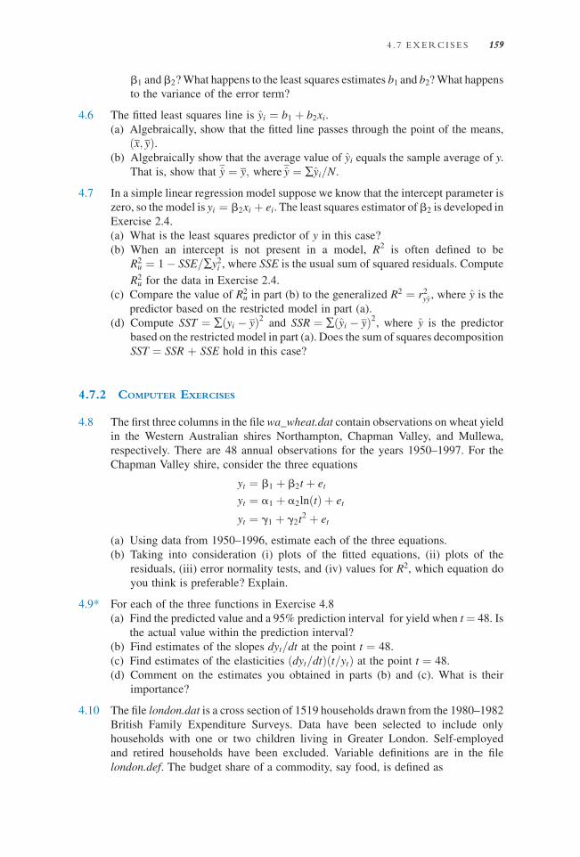
4.10 The file london.dat is a cross section of 1519 households drawn from the 1980–1982

British Family Expenditure Surveys. Data have been selected to include only

households with one or two children living in Greater London. Self-employed

and retired households have been excluded. Variable definitions are in the file

london.def. The budget share of a commodity, say food, is defined as

4 . 7 EXERCI SES 159

WFOOD ¼ expenditure on food

total expenditure

A functional form that has been popular for estimating expenditure functions for

commodities is

WFOOD ¼ b1 þ b2 lnðTOTEXPÞ þ e

(a) Estimate this function for households with one child and households with two

children. Report and comment on the results. (You may find it more convenient

to use the files lon1.dat and lon2.dat that contain the data for the one and two

children households, with 594 and 925 observations, respectively.)

(b) It can be shown that the expenditure elasticity for food is given by

e ¼ b1 þ b2½lnðTOTEXPÞ þ 1�b1 þ b2lnðTOTEXPÞ

Find estimates of this elasticity for one- and two-child households, evaluated at

average total expenditure in each case. Do these estimates suggest food is a

luxury or a necessity? (Hint: Are the elasticities greater than one or less than

one?)

(c) Analyze the residuals from each estimated function. Does the functional form

seem appropriate? Is it reasonable to assume that the errors are normally

distributed?

(d) Using the data on households with two children, lon2.dat, estimate budget share

equations for fuel (WFUEL) and transportation (WTRANS). For each equation

discuss the estimate of b2 and carry out a two-tail test of statistical significance.

(e) Using the regression results from part (d), compute the elasticity e for fuel andtransportation first at the median of total expenditure (90), and then at the 95th

percentile of total income (180). What differences do you observe? Are any

differences you observe consistent with economic reasoning?

4.11* Reconsider thepresidential votingdata (fair4.dat) introduced inExercises2.14and3.9.

(a) Using the data from 1916 to 2008, estimate the regression model

VOTE ¼ b1 þ b2GROWTH þ e. Based on these estimates, what is the predicted

value of VOTE in 2008? What is the least squares residual for the 2008 election

observation?

(b) Estimate the regression in (a) using the data from1916–2004. Predict thevalue of

VOTE in 2008 using the actual value of GROWTH for 2008, which was 0.22%.

What is the prediction error in this forecast? Is it larger or smaller than the error

computed in part (a)?

(c) Using the regression results from (b), construct a 95% prediction interval for

the 2008 value of VOTE using the actual value of GROWTH ¼ 0.22%. Is the

actual 2008 outcome within the prediction interval?

(d) Using the estimation results in (b), what value of GROWTH would have led to a

prediction that the incumbent party [Republicans] would havewon 50.1% of the

vote?

4.12 In Chapter 4.6 we considered the demand for edible chicken, which the U.S.

Department of Agriculture calls ‘‘broilers.’’ The data for this exercise are in the

file newbroiler.dat.

160 PRED ICT ION , GOODNESS -OF - F IT , AND MODEL ING I S SUES

(a) Using the 52 annual observations, 1950–2001, estimate the reciprocal model

Q ¼ a1 þ a2ð1=PÞ þ e. Plot the fitted value ofQ ¼ per capita consumption of

chicken, in pounds, versus P ¼ real price of chicken. How well does the

estimated relation fit the data?

(b) Using the estimated relation in part (a), compute the elasticity of per capita

consumption with respect to real price when the real price is its median, $1.31,

and quantity is taken to be the corresponding value on the fitted curve. [Hint: The

derivative (slope) of reciprocal model y ¼ a þ b(1=x) is dy=dx ¼ �b(1=x2)].Compare this estimated elasticity to the estimate found in Chapter 4.6 where the

log-log functional form was used.

(c) Estimate the poultry demand using the linear-log functional form

Q ¼ g1 þ g2 lnðPÞ þ e. Plot the fitted values of Q ¼ per capita consumption

of chicken, in pounds, versus P ¼ real price of chicken. How well does the

estimated relation fit the data?

(d) Using the estimated relation in part (c), compute the elasticity of per capita

consumption with respect to real price when the real price is its median, $1.31.

Compare this estimated elasticity to the estimate from the log-log model and

from the reciprocal model in part (b).

(e) Evaluate the suitability of the log-log, linear-log, and reciprocal models for fitting

the poultry consumption data. Which of them would you select as best, and why?

4.13* The file stockton2.dat contains data on 880 houses sold in Stockton, CA, duringmid-

2005. Variable descriptions are in the file stockton2.def. These data were considered

in Exercises 2.12 and 3.11.

(a) Estimate the log-linear model lnðPRICEÞ ¼ b1 þ b2SQFT þ e. Interpret the

estimated model parameters. Calculate the slope and elasticity at the sample

means, if necessary.

(b) Estimate the log-log model lnðPRICEÞ ¼ b1 þ b2lnðSQFTÞ þ e. Interpret the

estimated parameters. Calculate the slope and elasticity at the sample means, if

necessary.

(c) Compare the R2-value from the linear model PRICE ¼ b1 þ b2SQFT þ e to the

‘‘generalized’’ R2 measure for the models in (b) and (c).

(d) Construct histograms of the least squares residuals from each of the models in

(a), (b), and (c) and obtain the Jarque–Bera statistics. Based on your obser-

vations, do you consider the distributions of the residuals to be compatible with

an assumption of normality?

(e) For each of the models (a)–(c), plot the least squares residuals against SQFT. Do

you observe any patterns?

(f) For each model in (a)–(c), predict the value of a house with 2700 square feet.

(g) For each model in (a)–(c), construct a 95% prediction interval for the value of a

house with 2700 square feet.

(h) Based on your work in this problem, discuss the choice of functional form.

Which functional form would you use? Explain.

4.14 How much does education affect wage rates? This question will explore the issue

further. The data file cps4_small.dat contains 1000 observations on hourly wage

rates, education, and other variables from the 2008Current Population Survey (CPS).

(a) Construct histograms of theWAGE variable and its logarithm, ln(WAGE).Which

appears more normally distributed?

(b) Estimate the linear regression WAGE ¼ b1 þ b2EDUC þ e and log-linear

regression lnðWAGEÞ ¼ b1 þ b2EDUC þ e. What is the estimated return to

4 . 7 EXERCI SES 161