21712_04a.pdf
TRANSCRIPT

4 Additional Considerations for Thermal Design of Recuperators
The design theory for heat exchangers developed in Chapter 3 is based on the set of assumptions discussed in Section 3.2.1. That approach allows relatively straightforward solution of the corresponding design problems. In many applications, such design theory suffices and is used extensively. Still, some applications d o require inclusion of additional effects i.e., relaxation of a number of assumptions. In all these situations, however, the conventional theory generally fails. So, additional assumptions are necessary to modify the simplified approach or to devise a completely new design methodology.
In industry, heat exchanger design and analysis calculations are performed almost exclusively using commercial and/or proprietary computer software. These tools are equipped with sophisticated routines that can deal with real engineering designs, although they do not possess the transparency necessary for clearly guiding an engineer through the design process. To assess the order of magnitude of various influences, to analyze preliminary designs in a fast and flexible manner, and to involve engineering judgment in a most creative way, analytical and/or back-of-the-envelope approaches would be very helpful. These also require, however, insights into the additional influences beyond the basic assumptions mentioned above. Thus, it would be necessary to develop ways of assessing the effects not included in the basic design procedure covered in Chapter 3. In this chapter we consider the following enhancements to the basic design procedure: (1) longitudinal wall heat conduction effects in Section 4.1, (2) nonuniform heat transfer coefficients in Section 4.2, and (3) complex flow distributions in shell-and- tube heat exchangers in Section 4.4.
Additional considerations for completion of either a simplified design approach or one based on the relaxed assumptions are still necessary. Among these, the most impor- tant is the need to take into account the fin efficiency of extended heat transfer surfaces commonly used in compact heat exchangers and some shell-and-tube heat exchangers. Hence, considerable theory development and discussion is devoted to fin efficiency in Section 4.3.
4.1 LONGITUDINAL WALL HEAT CONDUCTION EFFECTS
In a heat exchanger, since heat transfer takes place, temperature gradients exist in both fluids and in the separating wall in the fluid flow directions. This results in heat conduc-
232

LONGITUDINAL WALL HEAT CONDUCTION EFFECTS 233
tion in the wall and in fluids from the hotter to colder temperature regions, which may affect the heat transfer rate from the hot fluid to the cold fluid.
Heat conduction in a fluid in the fluid flow direction is negligible for Pe > 10 and x* 2 0.005, where the Peclet number Pe = Re. Pr = U,,,Dh/Q and x* = X/(Dh . Pe); the significance and meaning of Pe and x* are presented in Section 7.2. For most heat exchangers, except liquid metal heat exchangers, Pe and x* are higher than the values indicated above. Hence, longitudinal heat conduction in the fluid is negligible in most applications and is not covered here.
If a temperature gradient is established in the separating walls between fluid flow streams in a heat exchanger, heat transfer by conduction takes place from the hotter to colder region of the wall, flattens the wall temperature distribution, and reduces the performance of the exchanger. For example, let us review typical temperature distribu- tions in the hot fluid, cold fluid, and wall for a counterflow heat exchanger as shown in Fig. 4.1. Dashed lines represent the case of zero longitudinal heat conduction, and solid lines represent the case of finite longitudinal conduction [A = 0.4, X defined in Eq. (4.13)]. From the figure it is clear that longitudinal conduction in the wall flattens the tempera- ture distributions, reduces the mean outlet temperature of the cold fluid, and thus reduces the exchanger effectiveness E from 90.9% to 73.1 %. This in turn produces a penalty in the exchanger overall heat transfer rate. The reduction in the exchanger effectiveness at a specified NTU may be quite significant in a single-pass exchanger having very steep temperature changes in the flow direction (i.e., large ATh/L or AT,/L). Such a situation arises for a compact exchanger designed for high effectiveness (approximately above 80%) and has a short flow length L. Shell-and-tube exchangers are usually designed for an exchanger effectiveness of 60% or below per pass. The influence of heat conduc- tion in the wall in the flow direction is negligible for such effectiveness.
Since the longitudinal wall heat conduction effect is important only for high-effec- tiveness single-pass compact heat exchangers, and since such exchangers are usually designed using E-NTU theory, we present the theory for the longitudinal conduction effect by an extension of E-NTU theory. No such extension is available in the MTD method.
The magnitude of longitudinal heat conduction in the wall depends on the wall heat conductance and the wall temperature gradient. The latter in turn depends on the thermal conductance on each side of the wall. To arrive at additional nondimensional groups for longitudinal conduction effects, we can work with the differential energy and rate equations of the problem and can derive the same Eq. (4.9) mentioned later. For example, see Section 5.4 for the derivation of appropriate equations for a rotary regen- erator. However, to provide a “feel” to the reader, a more heuristic approach is followed here. Let us consider the simple case of a linear temperature gradient in the wall as shown in Fig. 4.1. The longitudinal conduction rate is
where A k is total wall cross-sectional area for longitudinal conduction. The convective heat transfer from the hot fluid to the wall results in its enthalpy rate drop as follows, which is the same as enthalpy rate change (convection rate) q h :

234 ADDITIONAL CONSIDERATIONS FOR THERMAL DESIGN OF RECUPERATORS
0.0 0.1 0.2 0.3 0.4 0.5 0.6 0.7 0.8 0.9 1.0 Section 1 XlL Section 2
FIGURE 4.1 and finite longitudinal wall heat conduction.
Fluid and wall temperature distributions in a counterflow exchanger having zero
Similarly, the enthalpy rate rise of the cold fluid as a result of convection from the wall to the fluid is
Of course, q,, = qc, with no heat losses to the ambient. Therefore, the ratios of longitudinal heat conduction in the wall to the convection rates in the hot and cold fluids are
The resulting new dimensionless groups in Eqs. (4.4) and (4.5) are defined as
(4.4)
where for generality (for an exchanger with an arbitrary flow arrangement), the sub- scripts h and c are used for all quantities on the right-hand side of the equality sign of A’s.

LONGITUDINAL WALL HEAT CONDUCTION EFFECTS 235
The individual X is referred to as the longitudinal conduction parameter. It is defined as a ratio of longitudinal wall heat conduction per unit temperature difference and per unit length to the heat capacity rate of the fluid. Keeping in mind that relaxation of a zero longitudinal conduction idealization means the introduction of a new heat transfer pro- cess deterioration factor, we may conclude that the higher the value of X, the higher are heat conduction losses and the lower is the exchanger effectiveness compared to the X = 0 case.
Now considering the thermal circuit of Fig. 3.4 (with negligible wall thermal resis- tance and no fouling), the wall temperature at any given location can be given by Eq. (3.34) as
where
(4.7)
Hence, the wall temperature distribution is between Th and T, distributions, as shown in Fig. 4.1, and its specific location depends on the magnitude of (q,hA)*. If (vohA)* is zero (as in a condenser), T, = Th. And since Th is approximately constant for a condenser, T , will also be a constant, indicating no longitudinal temperature gradients in the wall, even though X will be finite. Thus, when (vohA)* is zero or infinity, the longitudinal heat conduction is zero. Longitudinal heat conduction effects are maximum for (qohA)* = 1.
Thus, in the presence of longitudinal heat conduction in the wall, we may expect and it can be proven that the exchanger effectiveness is a function of the following groups:
E = $[NTU, C*, Ahr A,, (qohA)*, flow arrangement] (4.9)
It should be added that the same holds for a parallelflow exchanger, but as shown in Section 4.1.3, longitudinal wall conduction effects for a parallelflow exchanger are neg- ligible. Note that for a counterflow exchanger,
Equation (4.6) then becomes
and therefore,
(4.1 1)
(4.12)
Thus for a counterflow exchanger, and A, are not both independent parameters since C* is already included in Eq. (4.9); only one of them is independent. Instead of choosing
236 ADDITIONAL CONSIDERATIONS FOR THERMAL DESIGN OF RECUPERATORS
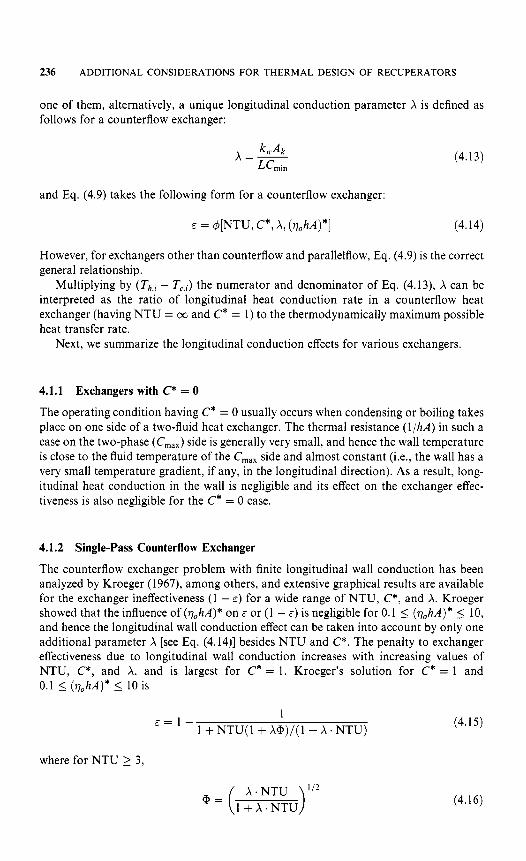
one of them, alternatively, a unique longitudinal conduction parameter X is defined as follows for a counterflow exchanger:
(4.13)
and Eq. (4.9) takes the following form for a counterflow exchanger:
E = $[NTU, C*, A, (qohA)*] (4.14)
However, for exchangers other than counterflow and parallelflow, Eq. (4.9) is the correct general relationship.
Multiplying by TI,,^ - Tc,i) the numerator and denominator of Eq. (4.13), X can be interpreted as the ratio of longitudinal heat conduction rate in a counterflow heat exchanger (having NTU = cc and C* = 1) to the thermodynamically maximum possible heat transfer rate.
Next, we summarize the longitudinal conduction effects for various exchangers.
4.1.1
The operating condition having C* = 0 usually occurs when condensing or boiling takes place on one side of a two-fluid heat exchanger. The thermal resistance (l/hA) in such a case on the two-phase (&,) side is generally very small, and hence the wall temperature is close to the fluid temperature of the C,,, side and almost constant (i.e., the wall has a very small temperature gradient, if any, in the longitudinal direction). As a result, long- itudinal heat conduction in the wall is negligible and its effect on the exchanger effec- tiveness is also negligible for the C* = 0 case.
Exchangers with C* = 0
4.1.2 Single-Pass Countertlow Exchanger
The counterflow exchanger problem with finite longitudinal wall conduction has been analyzed by Kroeger (1967), among others, and extensive graphical results are available for the exchanger ineffectiveness (1 - E ) for a wide range of NTU, C*, and A. Kroeger showed that the influence of (qokA)* on E or (1 - E ) is negligible for 0.1 5 (qohA)* 5 10, and hence the longitudinal wall conduction effect can be taken into account by only one additional parameter X [see Eq. (4.14)] besides NTU and C*. The penalty to exchanger effectiveness due to longitudinal wall conduction increases with increasing values of NTU, C*, and A, and is largest for C* = 1. Kroeger’s solution for C* = 1 and 0.1 5 (qohA)* 5 10 is
(4.15) 1
1 + NTU( 1 + A@)/ ( 1 + X . NTU) E = l -
where for NTU 2 3,
(4.16)
LONGITUDINAL WALL HEAT CONDUCTION EFFECTS 237
For X = 0 and 00, Eq. (4.15) reduces to
NTU/(1 + NTU) 1 [l - exp(-2NTU)]
for X = 0 for X = cc .=( (4.17)
Note that for X + 00, the counterflow exchanger effectiveness E from Eq. (4.17) is identical to E for a parallelflow exchanger (see Table 3.4). This is expected since the wall temperature distribution will be perfectly uniform for X + 00, and this is the case for a parallelflow exchanger with C* = 1.
For NTU + 00, Eq. (4.15) reduces to
(4.18) X & = 1 --
1 + 2 X
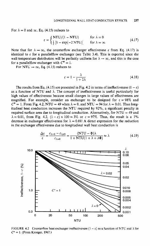
The results from Eq. (4.15) are presented in Fig. 4.2 in terms of ineffectiveness (1 - E )
as a function of NTU and A. The concept of ineffectiveness is useful particularly for high values of effectiveness because small changes in large values of effectiveness are magnified. For example, consider an exchanger to be designed for E = 98% and C* = 1. From Fig. 4.2, NTU = 49 when X = 0, and NTU = 94 for X = 0.01. Thus long- itudinal heat conduction increases the NTU required by 92%, a significant penalty in required surface area due to longitudinal conduction. Alternatively, for NTU = 49 and X = 0.01, from Fig. 4.2, (1 - E ) x 100 = 3% or E = 97%. Thus, the result is a 1% decrease in exchanger effectiveness for X = 0.01! A direct expression for the reduction in the exchanger effectiveness due to longitudinal wall heat conduction is
(4.19)
10.0
1 .o
0.3
- - 0 50 100 200 500
NTU
FIGURE 4.2 Counterflow heat exchanger ineffectiveness ( 1 - E ) as a function of NTU and X for C* = 1. (From Kroeger, 1967.)

238 ADDITIONAL CONSIDERATIONS FOR THERMAL DESIGN OF RECUPERATORS
for NTU large. In Eq. (4.19), the term on the right-hand side of the second equal sign is obtained from using Eq. (4.15) for X # 0 and Eq. (4.17) foi X = 0, and the last term on the right-hand side is obtained from Kays and London (1998).
The exchanger ineffectiveness for C* < 1 has been obtained and correlated by Kroeger (1967) as follows:
1-c* Q exp(rl) - P 1 - - E =
where
( I - C*)NTU 1 + A . NTU . C*
r I =
Q=- 1 +yQ* Q* = (CQ) "2 l + y 1 -yQ* I/. - y - y2
(4.20)
(4.21)
(3.22)
1 - c * 1 l + c * l + Q y=-- a = A . NTU. C* (4.23)
Note that here y and Q are local dimensionless variables as defined in Eq. (4.23). The values of Q are shown in Fig. 4.3. The approximate Eq. (4.20), although derived for (qohA)*/C* = 1, could be used for values of this parameter different from unity. For 0.5 < (q,hA)*/C* 5 2 , the error introduced in the ineffectiveness is within 0.8% and 4.7% for C* = 0.95 and 0.8, respectively.
1.6
1.5
1.4
JI 1.3
1.2
1.1
1 .o
I I I I I I I l l I I I I I I l l
0.10 1 .o h* NTU. C'
10.0
FIGURE 4.3 Function @ of Eq. (4.20) for computation of single-pass counterflow exchanger ineffectiveness, including longitudinal wall heat conduction effects. (From Kroeger, 1967.)

LONGITUDINAL WALL HEAT CONDUCTION EFFECTS 239
In summary, the decrease in exchanger effectiveness due to longitudinal wall heat conduction increases with increasing values of NTU, C* and A, and the decrease in E
is largest for C* = 1. Longitudinal wall conduction has a significant influence on the counterflow exchanger size (NTU) for a given E when NTU > 10 and X > 0.005.
4.1.3 Single-Pass Parallelflow Exchanger
In the case of a parallelflow exchanger, the wall temperature distribution is always almost close to constant regardless of the values of C* and NTU. Since the temperature gradient in the wall is negligibly small in the fluid flow direction, the influence of longitudinal wall conduction on exchanger effectiveness is negligible. Hence, there is no need to analyze or take this effect into consideration for parallelflow exchangers.
4.1.4 Single-Pass Unmixed-Unmixed Crossflow Exchanger
In this case, the temperature gradients in the wall iil the x and y directions of two fluid flows are different. This is because AT,,,,, and ATw,2 (AT,,l is the temperature difference in the wall occurring between inlet and outlet locations of fluid 1; similarly AT,,, is defined for fluid 2) are in general different, as well as Lh # L, in general. Hence, Ah and A, are independent parameters for a crossflow exchanger, and E is a function of five independent dimensionless groups, as shown in Eq. (4.9), when longitudinal wall heat conduction is considered. For the same NTU and C* values, the crossflow exchan- ger effectiveness is lower than the counterflow exchanger effectiveness; however, the wall temperature distribution is two-dimensional and results in higher temperature gradients for the crossflow exchanger compared to counterflow. Hence, for identical NTU, C*, and A, the effect of longitudinal conduction on the exchanger effectiveness is higher for the crossflow exchanger than that for the counterflow exchanger. Since crossflow exchangers are usually not designed for E 2 SO%, the longitudinal conduction effect is generally small and negligible compared to a counterflow exchanger that is designed for E up to 98 to 99%. Since the problem is more complicated for the crossflow exchanger, only the numerical results obtained by Chiou (published in Shah and Mueller, 1985) are presented in Table 4.1.
4.1.5 Other Single-Pass Exchangers
The influence of longitudinal conduction on exchanger effectiveness is not evaluated for recuperators of other flow arrangements. However, most single-pass exchangers with other flow arrangements are not designed with high effectiveness. hence there seems to be no real need for that information for such industrial heAt exchangers.
4.1.6 Multipass Exchangers
The influence of longitudinal conduction ip a multipass exchanger is evaluated indivi- dually for each pass, depending on the flow arrangement. The results of preceding sections are used for this purpose. Thus although the overall exchanger effectiveness may be quite high for an overall counterflow multipass unit, the individual pass effec- tiveness may not be high, and hence the influence of longitudinal conduction may not be significant for many multipass exchangers.

N PI 0
TABLE 4.1 Reduction in Crossflow Exchanger Effectiveness (A&/&) Due to Longitudinal Wall Heat Conduction for C* = I .
A E / E for A, = : -~ A, (%hA), E for AT ( ‘%h”)y NTU A, = 0 0.005 0.010 0.015 0.020 0.025 0.030 0.040 0.060 0.080 0.100 0.200 0.400
0.5 0.5 1 .oo 2.00 4.00 6.00 8.00
10.00 50.00
100.00
I .o 1 .oo 2.00 4.00 6.00 8.00
10.00 50.00
100.00
2.0 1 .oo 2.00 4.00 6.00 8.00
10.00 50.00
100.00
0.4764 0.6147 0.723 I 0.7729 0.803 I 0.8238 0.9229 0.9476
0.4764 0.6147 0.723 1 0.7729 0.803 1 0.8238 0.9229 0.9476
0.4764 0.6147 0.723 I 0.7729 0.803 I 0.8238 0.9229 0.9476
0.0032 0.0053 0.0080 0.0099 0.01 14 0.0127 0.0246 0.03 1 1
0.0029 0.0055 0.0078 0.0097 0.01 13 0.0125 0.0245 0.03 10
0.0027 0.0048 0.0076 0.0095 0.01 1 1 0.0124 0.0245 0.03 10
0.0062 0.0103 0.0156 0.0192 0.0220 0.0243 0.0446 0.0543
0.0055 0.0097 0.0151 0.0188 0.0217 0.0240 0.0445 0.0543
0.0051 0.0092 0.0147 0.0 I84 0.0214 0.0238 0.0444 0.0542
0.0089 0.0150 0.0227 0.0279 0.03 19 0.0351 0.0616 0.0732
0.0079 0.0141 0.0220 0.0273 0.0314 0.0347 0.0614 0.073 1
0.0074 0.0134 0.02 13 0.0268 0.0309 0.0343 0.06 13 0.073 I
0.0115 0.0194 0.0294 0.0360 0.041 1 0.0451 0.0764 0.0893
0.0102 0.0182 0.0284 0.0353 0.0404 0.0446 0.0763 0.0892
0.0095 0.0173 0.0277 0.0346 0.0398 0.0440 0.0761 0.0891
0.0 139 0.0236 0.0357 0.0437 0.0497 0.0545 0.0897 0.1034
0.0123 0.022 1 0.0346 0.0428 0.0489 0.0538 0.0895 0.1033
0.01 16 0.021 1 0.0336 0.0420 0.0482 0.0532 0.0893 0. I032
0.0 162 0.0276 0.04 18 0.05 10 0.0578 0.0633 0.1017 0.1160
0.0143 0.0258 0.0404 0.0499 0.0569 0.0624 0.1015 0.1159
0.0135 0.0247 0.0393 0.0490 0.0561 0.0617 0.1013 0.1158
0.0204 0.0350 0.0530 0.0644 0.0728 0.0793 0.1229 0.1379
0.0180 0.0327 0.0512 0.0630 0.0716 0.0782 0.1226 0. I378
0.0170 0.03 13 0.0499 0.0619 0.0706 0.0774 0.1223 0.1377
0.0276 0.048 1 0.0726 0.0877 0.0984 0.1066 0.1569 0.1729
0.0244 0.0449 0.0702 0.0857 0.0968 0.1052 0.1566 0.1727
0.0232 0.0432 0.0685 0.0844 0.0956 0.1041 0. I563 0.1725
0.0336 0.0592 0.0892 0.1072 0.1197 0.1290 0.1838 0.2001
0.0296 0.0553 0.0863 0.1049 0.1 178 0.1274 0.1834 0.1999
0.0285 0.0533 0.0844 0.1033 0.1164 0.1262 0.1831 0. I997
0.0387 0.0689 0.1036 0.1239 0.1377 0.1480 0.2057 0.2223
0.0341 0.0643 0.1002 0.1213 0.1356 0.1462 0.2053 0.2221
0.0330 0.0621 0.0982 0.1196 0. I342 0.1450 0.2050 0.2219
0.0558 0.1026 0.1535 0.1810 0.1988 0.21 15 0.2765 0.2942
0.0490 0.0959 0.1491 0.1779 0.1965 0.2096 0.2758 0.2933
0.0489 0.0938 0.1468 0.1760 0. I949 0.2083 0.2754 0.2928
0.0720 0.1367 0.2036 0.2372 0.2580 0.2724 0.3427 0.3666
0.0634 0.1286 0.1991 0.2344 0.2560 0.2708 0.3405 0.3619
0.0652 0. I274 0.1971 0.2328 0.2548 0.2698 0.3401 0.3600

1.0 0.5 1.00 2.00 4.00 6.00 8.00
10.00 50.00
100.00
1.0 1.00 2.00 4.00 6.00 0.00
10.00 50.00
100.00
2.0 1.00 2.00 4.00 6.00 8.00
10.00 50.00
100.00
0.4764 0.6147 0.7231 0.7729 0.8031 0.8238 0.9229 0.9476
0.4764 0.6147 0.723 1 0.7729 0.8031 0.8238 0.9229 0.9476
0.4764 0.6147 0.7231 0.7729 0.8031 0.8238 0.9229 0.9476
0.0020 0.0034 0.0053 0.0066 0.0076 0.0085 0.0170 0.0218
0.0020 0.0034 0.0053 0.0066 0.0076 0.0085 0.0170 0.0218
0.0020 0.0034 0.0053 0.0066 0.0076 0.0085 0.0170 0.0218
0.0039 0.0067 0.0103 0.0129 0.0148 0.0165 0.0316 0.0395
0.0038 0.0066 0.0103 0.0129 0.0149 0.0165 0.0316 0.0395
0.0039 0.0067 0.0103 0.0 I29 0.0148 0.0165 0.0316 0.0395
0.0057 0.0098 0.0152 0.0189 0.0217 0.0241 0.0445 0.0543
0.0055 0.0097 0.0152 0.0189 0.0217 0.0241 0.0445 0.0543
0.0057 0.0098 0.0152 0.0189 0.0217 0.0241 0.0445 0.0543
0.0074 0.0128 0.0198 0.0246 0.0283 0.03 13 0.0562 0.0673
0.0072 0.0 I27 0.0198 0.0246 0.0283 0.03 13 0.0562 0.0673
0.0074 0.0128 0.0198 0.0246 0.0283 0.03 13 0.0562 0.0673
0.0090 0.0157 0.0243 0.0302 0.0346 0.0382 0.0667 0.0789
0.0088 0.01 56 0.0243 0.0301 0.0346 0.0382 0.0667 0.0789
0.0090 0.0157 0.0243 0.0302 0.0346 0.0382 0.0667 0.0789
0.0106 0.0185 0.0287 0.0355 0.0406 0.0448 0.0765 0.0894
0.0103 0.0183 0.0286 0.0354 0.0406 0.0448 0.0765 0.0894
0.0106 0.0185 0.0287 0.0355 0.0406 0.0448 0.0765 0.0894
0.0136 0.0238 0.0369 0.0456 0.0520 0.0571 0.0940 0.1080
0.0132 0.0236 0.0368 0.0455 0.0519 0.0571 0.0940 0.1080
0.0136 0.0238 0.0369 0.0456 0.0520 0.0571 0.0940 0.1080
0.0190 0.0336 0.0520 0.0637 0.0723 0.0790 0.1233 0.1385
0.0183 0.033 I 0.0517 0.0636 0.0722 0.0789 0.1233 0.1385
0.0190 0.0336 0.0520 0.0637 0.0723 0.0790 0.1233 0.1385
0.0237 0.0423 0.0653 0.0797 0.0900 0.0979 0.1474 0.1632
0.0228 0.0417 0.0650 0.0795 0.0898 0.0978 0.1473 0.1632
0.0237 0.0423 0.0653 0.0797 0.0900 0.0979 0.1474 0.1632
0.0280 0.0501 0.0773 0.0940 0.1057 0.1145 0.1677 0.1840
0.0268 0.0493 0.0769 0.0936 0.1054 0.1 143 0.1677 0.1840
0.0280 0.0501 0.0773 0.0940 0.1057 0.1145 0.1677 0.1840
0.0436 0.0609 0.0803 0.1 154 0.1229 0.1753 0.1472 0.2070 0.1634 0.2270 0.1751 0.2410 0.2378 0.3092 0.2546 0.3273
0.0412 0.0567 0.0786 0.1 125 0.1220 0.1742 0.1466 0.2064 0.1630 0.2266 0.1749 0.2407 0.2377 0.3090 0.2546 0.3270
0.0436 0.0609 0.0803 0.1 154 0.1229 0.1753 0.1472 0.2070 0.1634 0.2270 0.1751 0.2410 0.2378 0.3092 0.2546 0.3273
(continued)
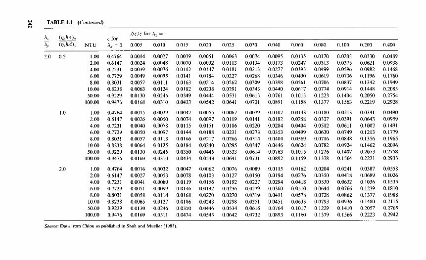
TABLE 4.1 (Continued). ..
AEJE for A, = : - _ _ A, ( V o h 4 , c for A,, (%$A), NTU A, = 0 0.005 0.010 0.015 0.020 0.025 0.030 0.040 0.060 0.080 0.100 0.200 0.400
2.0 0.5 1 .00 2.00 4.00 6.00 8.00
10.00 50.00
100.00
1 .0 1 .00 2.00 4.00 6.00 8.00
10.00 50.00
100.00
2.0 1 .00 2.00 4.00
8.00
50.00 100.00
6.00
io.no
0.4764 0.6147 0.723 1 0.7729 0.8031 0.8238 0.9229 0.9476
0.4764 0.6147 0.7231 0.7729 0.8031 0.8238 0.9229 0.9476
0.4764 0.6147 0.723 1 0.7729 0.803 1 0.8238 0.9229 0.9476
0.0014 0.0024 0.0039 0.0049 0.0057 0.0063 0.0130 0.0168
0.0015 0.0026 0.0040 0.0050 0.0057 0.0064 0.01 30 0.0169
0.0016 0.0027 0.0041 0.0051 0.0058 0.0065 0.0130 0.0169
0.0027
0.0076 0.0095 0.01 11 0.0124 0.0245 0.0310
0.0029
0.0078 0.0097 0.01 13 0.0125 0.0245 0.0310
0.0032 0.0053 0.0080 0.0099 0.01 14 0.0127 0.0246 0.031 1
0.0048
0.0050
0.0039
0.01 12 0.0141 0.0 163 0.0182 0.0349 0.0433
0.0042 0.0074 0.0115 0.0144 0.0166 0.01 84 0.0350 0.0434
0.0047 0.0078 0.01 19 0.0146 0.0168 0.0186 0.0350 0.0434
0.0070 0.0051 0.0092 0.0147 0.0 184 0.0214 0.0238 0.0444 0.0542
0.0055 0.0097 0.0151 0.01 88 0.02 17 0.0240 0.0445 0.0543
0.0062 0.0103 0.0156 0.0192 0.0220 0.0243 0.0446 0.0543
0.0063 0.01 13 0.0181 0.0227 0.0262 0.0291 0.0531 0.0641
0.0067 0.01 19 0.0186 0.0231 0.0266 0.0295 0.0533 0.0641
0.0076 0.0127 0.0 192 0.0236 0.0270 0.0298 0.0534 0.0642
0.0074 0.0134 0.0213 0.0268 0.0309 0.0343 0.0613 0.0731
0.0079 0.0141 0.0220 0.0273 0.0314 0.0347 0.0614 0.0731
0.0089 0.0 150 0.0227 0.0279 0.0319 0.0351 0.0616 0.0732
0.0095 0.0 I73 0.0277 0.0346 0.0398 0.0440 0.0761 0.0891
0.0102 0.0182 0.0284 0.0353 0.0404
0.0563 0.0892
0.0115 0.0194 0.0294 0.0360 0.041 I 0.0451 0.0764 0.0893
0.0446
0.0135 0.0247 0.0393 0.0490 0.0561 0.06!7 0.1013 0.1158
0.0143 0.0258 0.0404 0.0499 0.0569 0.0624 0.1015 0.1159
0.0 I62 0.0276 0.0418 0.0510 0.0578 0.0633 0.1017 0.1 160
0.0170 0.0313 0.0499
0.0706 0.0774 0.1223 0.1377
0.0180
0.05 12 0.0630 0.0716 0.0782 0.1226 0.1378
0.0204 0.0350 0.0530 0.0644 0.0728 0.0793 0.1229 0.1379
0.0619
0.0327
0.0203 0.0375 0.0596 0.0736 0.0837 0.0914 0.1404 0.1563
0.0213 0.0391 0.061 1 0.0749 0.0848 0.0924 0.1407 0.1564
0.0241 0.0418 0.0632 0.0766 0.0862 0.0936 0.1410 0. I566
0.0330 0.062 I 0.0982 0.1196 0.1342 0.1448 0.2050 0.2219
0.0341 0.0643 0.1002 0.1213 0.1356 0.1462 0.2053 0.2221
0.0387 0.0689 0.1036 0.1239 0.1377 0.1480 0.2057 0.2223
0.0489 0.0938 0.1468 0.1760 0.1949 0.2083 0.2754 0.2928
0.0490 0.0959 0.1491 0.1779 0.1965 0.2096 0.2758 0.2933
0.0558 0.1026 0.1535 0.1810 0.1988 0.21 15 0.2765 0.2942
Source: Data from Chiou as published in Shah and Mueller (1985).

LONGITUDINAL WALL HEAT CONDUCTION EFFECTS 343
Example 4.1 A gas-to-air crossflow waste heat recovery exchanger, having both fluids unmixed, has NTU = 6 and C* = 1. The inlet fluid temperatures on the hot and cold sides are 360°C and 25"C, respectively. Determine the outlet fluid temperatures with and without longitudinal wall heat conduction. Assume that A, = Ah = 0.04, and (vohA)h/(vohA)c = 1.
SOLUTION
Problem Data and Schematic: NTU, ratio of heat capacity rates, inlet temperatures, and hot- and cold-side A's are given for a crossflow gas-to-air waste heat recovery exchanger (Fig. E4.1).
Determine: The outlet temperatures with and without longitudinal wall heat conduction.
Assumptions: Fluid properties are constant and the longitudinal conduction factor X is also constant throughout the exchanger.
Analysis: In the absence of longitudinal conduction (i.e., A, = 0), we could find the effectiveness E = 0.7729 from Table 4.1 or Eq. (11.1) of Table 3.6. Using the definition of E , the outlet temperatures are
Th,o = Th,j-E(Th,i - T,j) = 360°C - 0.7729(360 - 25)"C = 101.1"c AnS.
T,,o = Tc,i f E ( Th,i - TQ) = 25°C + 0.7729(360 - 25)"C = 283.9"C Ans.
To take longitudinal conduction into account, we need to find the new effectiveness of the exchanger. Knowing that NTU = 6, C* = 1, & / A h = 1, and A, = 0.04, from Table 4.1 we have A€/€ = 0.0455. Therefore, the new effectiveness, using the expressions of the first equality of Eq. (4.19), is
= (1 - = (1 - 0.0445)0.7729 = 0.7377
360°C - t
25°C
FIGURE E4.1
244 ADDITIONAL CONSIDERATIONS FOR THERMAL DESIGN OF RECUPERATORS
Thus, from the definition of effectiveness, the outlet temperatures are
Th,o = Th,r - E ( T ~ , ~ - Tc, f ) = 360°C - 0.7377(360 - 25)"C = 112.9"C
Tc,o = Tc,I + E(T,~,, - Tc,l) = 25°C + 0.7377(360 - 25)"C = 272.1"C
Ans.
An$.
Discussion and Comments: For this particular problem, the reduction in exchanger effec- tiveness is quite serious, 4.6%, with corresponding differences in the outlet temperatures. This results in a 4.6% reduction in heat transfer or a 4.6% increase in fuel consumption to make up for the effect of longitudinal wall heat conduction. This example implies that for some high-effectiveness crossflow exchangers, longitudinal wall heat conduction may be important and cannot be ignored. So always make a practice of considering the effect of longitudinal conduction in heat exchangers having E 2 75% for single-pass units or for individual passes of a multiple-pass exchanger.
4.2 NONUNIFORM OVERALL HEAT TRANSFER COEFFICIENTS
In E-NTU, P-NTU, and MTD methods of exchanger heat transfer analysis, it is idealized that the overall heat transfer coefficient U is constant and uniform throughout the exchanger and invariant with time. As discussed for Eq. (3.24), this U is dependent on the number of thermal resistances in series, and in particular, on heat transfer coefficients on fluid 1 and 2 sides. These individual heat transfer coefficients may vary with flow Reynolds number, heat transfer surface geometry, fluid thermophysical properties, entrance length effect due to developing thermal boundary layers, and other factors. In a viscous liquid exchanger, a tenfold variation in h is possible when the flow pattern encompasses laminar, transition, and turbulent regions on one side. Thus, if the indivi- dual h values vary across the exchanger surface area, it is highly likely that U will not remain constant and uniform in the exchanger.
Now we focus on the variation in U and how to take into account its effect on exchanger performance considering local heat transfer coefficients on each fluid side varying slightly or significantly due to two effects: (1) changes in the fluid properties or radiation as a result of a rise in or drop of fluid temperatures, and (2) developing thermal boundary layers (referred to as the length efect) . In short, we relax assumption 8 postulated in Section 3.2.1 that the individual and overall heat transfer coefficients are constant.
The first effect, due to fluid property variations (or radiation), consists of two com- ponents: (1) distortion of velocity and temperature profiles at a given free flow cross section due to fluid property variations (this effect is usually taken into account by the property ratio method, discussed in Section 7.6); and (2) variations in the fluid tempera- ture along axial and transverse directions in the exchanger, depending on the exchanger flow arrangement; this effect is referred to as the temperature effect. The resulting axial changes in the overall mean heat transfer coefficient can be significant; the variations in U,,,,, could be nonlinear, depending on the type of fluid. While both the temperature and thermal entry length effects could be significant in laminar flows, the latter effect is generally not significant in turbulent flow except for low-Prandtl-number fluids.
It should be mentioned that in general the local heat transfer coefficient in a heat exchanger is also dependent on variables other than the temperature and length effects, such as flow maldistribution, fouling, and manufacturing imperfections. Similarly, the

NONUNIFORM OVERALL HEAT TRANSFER COEFFICIENTS 245
overall heat transfer coefficient is dependent on heat transfer surface geometry, indivi- dual Nu (as a function of relevant parameters), thermal properties, fouling effects, tem- perature variations, temperature difference variations, and so on. No information is available on the effect of some of these parameters, and it is beyond the scope of this book to discuss the effect of other parameters. In this section we concentrate on non- uniformities in U due to temperature and length effects.
To outline how to take temperature and length effects into account, let us introduce specific definitions of local and mean overall heat transfer coefficients. The local overall heat transfer coefficient U(xf, xt, T ) , is defined as follows in an exchanger at a local position [x* = x / (Dh . R e . Pr), subscripts 1 and 2 for fluids 1 and 21 having surface area dA and local temperature difference ( Th - T,) = AT:
u=- dq dA AT
(4.24)
Traditionally, the mean overall heat transfer coefficient Urn( T ) is defined as
Here fouling resistances and other resistances are not included for simplifying the dis- cussion but can easily be included if desired in the same way as in Eq. (3.24). In Eq. (4.25), the h,’s are the mean heat transfer coefficients obtained from the experimental/empirical correlations, and hence represent the surface area average values. The experimental/ empirical correlations are generally constant fluid property correlations, as explained in Section 7.5. If the temperature variations and subsequent fluid property variations are not significant in the exchanger, the reference temperature Tin U,(T) for fluid properties is usually the arithmetic mean of inlet and outlet fluid temperatures on each fluid side for determining individual h,’s; and in some cases, this reference temperature T is the log- mean average temperature on one fluid side, as discussed in Section 9.1, or an integral- mean average temperature. If the fluid property variations are significant on one or both fluid sides, the foregoing approach is not adequate.
A more rigorous approach is the area average U used in the definition of NTU [see the first equality in Eq. (3.59)], defined as follows:
(4.26)
This definition takes into account exactly both the temperature and length effects for counterflow and parallelflow exchangers, regardless of the size of the effects. However, there may not be possible to have a closed-form expression for U ( x , y ) for integration. Also, no rigorous proof is available that Eq. (4.26) is exact for other exchanger flow arrangements.
When both the temperature and length effects are not negligible, Eq. (4.24) needs to be integrated to obtain an overall 8 (which takes into account the temperature and length effects) that can be used in conventional heat exchanger design. The most accurate approach is to integrate Eq. (4.24) numerically for a given problem. However, if we can come up with some reasonably accurate value of the overall 8 after approximately

246 ADDITIONAL CONSIDERATIONS FOR THERMAL DESIGN OF RECUPERATORS
integrating Eq. (4.24), it will-allow us to use the conventional heat exchanger design methods with U replaced by u.
Therefore, when either one or both of the temperature and length effects are not negligible, we need to integrate Eq. (4.24) approximately as follows. Idealize local U(x,y, T) = Vrn(T)f(x,y) and U ( X ~ , X ~ , T) = U,(T)f(x:,x~); here Urn(T) is a pure temperature function and f(x,y) = f(x7,xz) is a pure position function. Hence, Eq. (4.24) reduces to
(4.27)
and integrate it as follows:
An overall heat transfer coefficient 0 that takes the temperature effect into account exactly for a counterflow exchanger is given by the first equality of the following equa- tion, obtained by Roetzel as reported by Shah and SekuliC (1998):
Note that V ( T ) = Urn( T ) in Eq. (4.29) depends only on local temperatures on each fluid side and is evaluated using Eq. (4.25) locally. The approximate equality sign in Eq. (4.29) indicates that the counterflow temperature effect is valid for any other exchanger flow arrangement considering it as hypothetical counterflow, so that AT, and ATII are evaluated using Eq. (3.173).
The overall heat transfer coefficient Urn( T ) on the left-hand side of Eq. (4.28) depends on the temperature only. Let us write the left-hand side of Eq. (4.28) by definition in the following foim:
(4.30)
Thus, this equation defines 0 which takes into account the temperature effect only. The integral on the right-hand side of Eq. (4.30) is replaced by the definition of true mean temperature difference (MTD) as follows:
(4.31)
Integration of the right-hand side of Eq. (4.28) yields the definition of a correction factor n that takes into account the length effect on the overall heat transfer coefficient.
(4.32)
where x: and xz are the dimensionless axial lengths for fluids 1 and 2, as noted earlier.

NONUNIFORM OVERALL HEAT TRANSFER COEFFICIENTS 247
Finally, substituting the results from Eqs. (4.30H4.32) into Eq. (4.28) and re- arranging yields
9 = O.A AT, =CA AT, (4.33)
Thus, an overall heat transfer coefficient ture (0) and length effects (.) is given by
which takes into account both the tempera-
G = - U , ( T ) f ( x , y ) d A = 06 A ‘ J (4.34)
As noted before, f (x, y ) = f ( x 7 , xg) is a pure position function. We provide appropriate formulas for 0 and K. in the following sections. Note that since K. 5 1 (see Fig. 4 . 9 ,
5 0. Also from Eq. (4.30) we find that 0 = U,,, if the temperature effect is not significant (i.e., Um(T) does not vary significantly with r).
It can be shown that for a counterflow exchanger, - - U = O = f i (4.35)
with 6 defined by Eq. (4.26) and 0 defined by Eq. (4.29) with U ( x , T) instead of U ( T) or Um(T). Hence, for evaluating 0 for a counterflow exchanger, one can use 6, which is a function of only the area (flow length), such as for laminar gas flows, or 0, which is a function of the temperature only such as for turbulent liquid flows. These different definitions of overall heat transfer coefficients are summarized in Table 4.2.
TABLE 4.2 Definitions of Local and Mean Overall Heat Transfer Coefficients
Symbol Definition Comments
U dq Basic definition of the local overall heat .!,I=- dA AT transfer coefficient.
ri O = z U ( A ) d A ’ J A
Overall heat transfer coefficient defined using area average heat transfer coefficients on both sides. Individual heat transfer coefficients should be evaluated at respective reference temperatures (usually arithmetic mean of inlet and outlet fluid temperatures on each fluid side).
Mean overall heat transfer coefficient averaged over heat transfer surface area.
Mean overall heat transfer coefficient that takes into account the temperature effect only.
0 0 = (InAT, - InAT,)
Mean overall heat transfer coefficient that takes into account the temperature and length effects. The correction factor K takes into account the entry length effect.
248 ADDITIONAL CONSIDERATIONS FOR THERMAL DESIGN OF RECUPERATORS
Now y e discuss methods that take temperature and length effects into account, to arrive at for the exchanger analysis.
4.2.1 Temperature Effect
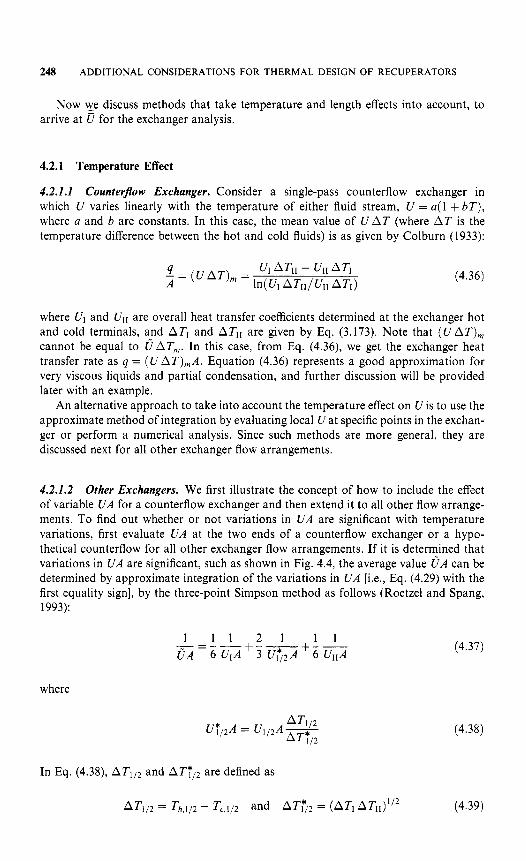
4.2.1.1 Counterflow Exchanger. Consider a single-pass counterflow exchanger in which U varies linearly with the temperature of either fluid stream, U = u( 1 + b T ) , where a and b are constants. In this case, the mean value of U A T (where A T is the temperature difference between the hot and cold fluids) is as given by Colburn (1933):
(4.36)
where UI and UII are overall heat transfer coefficients determined at the exchanger hot and cold terminals, and A T , and AT,, are given by Eq. (3.173). Note that ( U A T ) , cannot be equal to OAT,. In this case, from Eq. (4.36), we get the exchanger heat transfer rate as q = ( U AT),,A. Equation (4.36) represents a good approximation for very viscous liquids and partial condensation, and further discussion will be provided later with an example.
An alternative approach to take into account the temperature effect on U is to use the approximate method of integration by evaluating local U at specific points in the exchan- ger or perform a numerical analysis. Since such methods are more general, they are discussed next for all other exchanger flow arrangements.
4.2.1.2 Other Exchangers. We first illustrate the concept of how to include the effect of variable UA for a counterflow exchanger and then extend it to all other flow arrange- ments. To find out whether or not variations in U A are significant with temperature variations, first evaluate U A at the two ends of a counterflow exchanger or a hypo- thetical counterflow for all other exchanger flow arrangements. If it is determined that variations in UA are significant, such as shown in Fig. 4.4, the average value O A can be determined by approximate integration of the variations in UA [i.e., Eq. (4.29) with the first equality sign], by the three-point Simpson method as follows (Roetzel and Spang, 1993):
where
In Eq. (4.38), A T l l z and ATy12 are defined as
(4.37)
(4.38)
ATI12 = Th,]12 - T c , l ~ 2 and = ( A T , ATl I ) ' / ' (4.39)

NONUNIFORM OVERALL HEAT TRANSFER COEFFICIENTS 249
t
i l A I I I I Y1/2 I Y2 I I y 1 I I -
X1 x1/2 x2
FIGURE 4.4 Variable U A in a counterflow exchanger for the Simpson method.
where the subscripts I and I1 correspond to terminal points at the end sections, and the subscript corresponds to a point in between defined by the second equation, respec- tively. Here Th,1/2 and Tc,l/2 are computed through the procedure of Eqs. (4.43H4.45).
Usually, uncertainty in the individual heat transfer coefficient is high, so that the three-point approximation may be sufficient in most cases. Note that for simplicity, we have selected the third point as the middle point in the example above. The middle point is defined in terms of ATI and AT11 [defined by Eq. (3.173)] to take the temperature effect properly into account; it is not a physical middle point along the length of the exchanger. The step-by-step procedure that involves this approach is presented in Section 4.2.3.1.
4.2.2 Length Effect
The heat transfer coefficient can vary significantly in the entrance region of laminar flow. This effect is negligible for turbulent flows. Hence, we associate the length effect to laminar flow. For hydrodynamically developed and thermally developing flow, the local and mean heat transfer coefficients h, and h, for a circular tube or parallel plates are related as follows (Shah and London, 1978):
h, = 3 h m ( X * ) - " 3 (4.40)
where x* = x/(Dh . Re . Pr). Using this variation in h on one or both fluid sides, counter- flow and crossflow exchangers have been analyzed, and the correction factors r; are presented in Fig. 4.5 and Table 4.3 as a function of pI or p2, where
The value of K is 0.89 for pI = 1, (i.e., when the exchanger has the hot- and cold-side thermal resistances approximately balanced and R, = 0). Thus, when a vadation in the heat tgnsfer coefficient due to the thermal entry length effect is considered, 5 0 or U, since D = from Eq. (4.34). This can be explained easily if one considers the thermal resistances connected in series for the problem. For example, consider a very simplified problem with the heat transfer coefficient on each fluid side of a counterflow exchanger

250 ADDITIONAL CONSIDERATIONS FOR THERMAL DESIGN OF RECUPERATORS
0.98
0.96
k 0.94
0.92
0.90
0.88 0.1 0.2 0.5 1 2 5 10
Q
FIGURE 4.5 Length effect correction factor K for one and both laminar streams based on equations in Table 4.3 (From Roetzel, 1974).
varying from 80 to 40 W / m 2 . K from entrance to exit and A , = A 2 , R,,. = 0, qO,, = Q , , ~ = 1, and there is no temperature effect. In this case, the arithmetic average hn,,l = h,n,2 = 60 W / m 2 . K and Urn = 30 W / m 2 . K. However, a t each end of this counterlow exchanger, Ul = U2 = 26.61 W/m:. K (since 1 /U = 1/80 + 1/40). Hence u = ( U , + U2)/2 = 26.67 W/m2 . K. Thus u / U m = 26.67130 = 0.89.
TABLE 4.3 Length Effect Correction Factor K When One or Both Streams Are in Laminar Flow for Various Exchanger Flow Arrangements
One stream laminar counterflow, parallelflow, crossflow, 1-2n TEMA E
Both streams laminar Counterflow
Crossflow
0.65 + 0.23R,(al + a 2 ) 4.1 + al/a2 + a2/al + 3R,,(al + a2) + 2Rt.ala2
K = l -
0.44 + 0.23R,, (al + a2) 4.1 + a l /a2 + a2/al + 3R,,.(al + a2) + 2Rtalaz
K = t -
NONUNIFORM OVERALL HEAT TRANSFER COEFFICIENTS 251
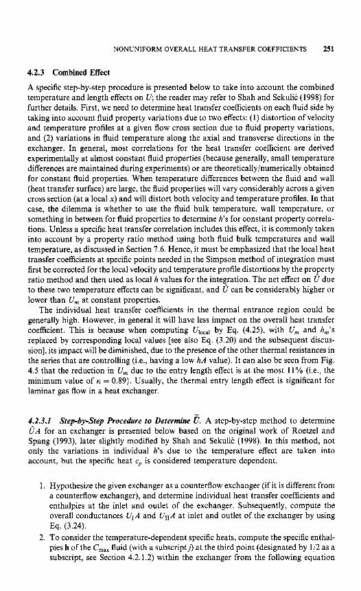
4.2.3 Combined Effect
A specific step-by-step procedure is presented below to take into account the combined temperature and length effects on U; the reader may refer to Shah and Sekulii: (1998) for further details. First, we need to determine heat transfer coefficients on each fluid side by taking into account fluid property variations due to two effects: (1) distortion of velocity and temperature profiles at a given flow cross section due to fluid property variations, and (2) variations in fluid temperature along the axial and transverse directions in the exchanger. In general, most correlations for the heat transfer coefficient are derived experimentally at almost constant fluid properties (because generally, small temperature differences are maintained during experiments) or are theoretically/numerically obtained for constant fluid properties. When temperature differences between the fluid and wall (heat transfer surface) are large, the fluid properties will vary considerably across a given cross section (at a local x ) and will distort both velocity and temperature profiles. In that case, the dilemma is whether to use the fluid bulk temperature, wall temperature, or something in between for fluid properties to determine h’s for constant property correla- tions. Unless a specific heat transfer correlation includes this effect, it is commonly taken into account by a property ratio method using both fluid bulk temperatures and wall temperature, as discussed in Section 7.6. Hence, it must be emphasized that the local heat transfer coefficients at specific points needed in the Simpson method of integration must first be corrected for the local velocity and temperature profile distortions by the property ratio method and then used as local h values for the integration. The net effect on 0 due to these two temperature effects can be significant, and 0 can be considerably higher or lower than Urn at constant properties.
The individual heat transfer coefficients in the thermal entrance region could be generally high. However, in general it will have less impact on the overall heat transfer coefficient. This is because when computing Ulocal by Eq. (4.25), with Urn and h,’s replaced by corresponding local values [see also Eq. (3.20) and the subsequent discus- sion], its impact will be diminished, due to the presence of the other thermal resistances in the series that are controlling (i.e., having a low hA value). It can also be seen from Fig. 4.5 that the reduction in Urn due to the entry length effect is at the most 11% (i.e., the minimum value of IC = 0.89). Usually, the thermal entry length effect is significant for laminar gas flow in a heat exchanger.
4.2.3.1 Step-by-Step Procedure to Determine c. A step-by-step method to determine 0 A for an exchanger is presented below based on the original work of Roetzel and Spang (1993), later slightly modified by Shah and Sekulic (1998). In this method, not only the variations in individual h’s due to the temperature effect are taken into account, but the specific heat cp is considered temperature dependent.
1. Hypothesize the given exchanger as a counterflow exchanger (if it is different from a counterflow exchanger), and determine individual heat transfer coefficients and enthalpies at the inlet and outlet of the exchanger. Subsequently, compute the overall conductances U I A and UllA at inlet and outlet of the exchanger by using Eq. (3.24).
2. To consider the temperature-dependent specific heats, compute the specific enthal- pies h of the C,,, fluid (with a subscript]] at the third point (designated by 1/2 as a subscript, see Section 4.2.1.2) within the exchanger from the following equation

252 ADDITIONAL CONSIDERATIONS FOR THERMAL DESIGN OF RECUPERATORS
using the known values a t each end:
(4.42)
where is given by
ATT/2 = (AT1 ATII)’” (4.43)
Here AT, = (Th - T,), and AT,, = (T18 - Tc)II. If AT1 = AT,,, (i.e., C* = R I = l), the rightmost bracketed term in Eq. (4.42) becomes 1/2. If the specific heat is constant, the enthalpies can be replaced by temperatures in Eq. (4.42). If the specific heat does not vary significantly, Eq. (4.42) could also be used for the Cmin fluid. However, when it varies significantly as in a cryogenic heat exchanger, the third point calculated for the C,,, and Cmin fluid by Eq. (4.42) will not be close enough in the exchanger (Shah and SekuliC, 1998). In that case, compute the third point for the Cmin fluid by the energy balance as follows:
Subsequently, using the equation of state or tabular/graphical results, determine the temperature Th,l/2 and T,,l/2 corresponding to hh,1/2 and hc,1/2. Then
AT112 = Th.I/2 - T 4 2 (4.45)
3. For a counterflow exchanger, the heat transfer coefficient hj,1/2 on each fluid side at the third point is calculated based on the temperatures T,,l/2 determined in the preceding step. For other exchangers, compute hj,l/2 at the following corrected reference (Roetzel and Spang, 1993):
(4.46)
(4.47)
In Eqs. (4.46) and (4.47), F is the log-mean temperature difference correction factor and Rh = ch/c, or R, = c,/ch. The temperatures Th,l12,corr and Tc,l12,corr are used only for the evaluation of fluid properties to compute hh.l/2 and h,,l/2. The foregoing correction to the reference temperature T/,,/2 ( j = h or c) results in the cold temperature being increased and the hot temperature being decreased.
Calculate the overall conductance at the third point by
(4.48) 1 + Rbv + 1 - 1 U1/2A- r]0,h~h,l/2~h %,chc,l/2A,
Note that qf and v0 can be determined accurately at local temperatures.

NONUNIFORM OVERALL HEAT TRANSFER COEFFICIENTS 253
4. Calculate the apparent overall heat transfer coefficient at this third point using Eq. (4.38):
(4.49)
5. Find the mean overall conductance for the exchanger (taking into account the temperature dependency of the heat transfer coefficient and heat capacities) from the equation
(4.50)
6. Finally, the true mean heat transfer coefficient b that also takes into account the laminar flow entry length effect is given by
FA = OAn (4.51)
where the entry length effect factor n 5 1 is given in Fig. 4.5 and Table 4.3.
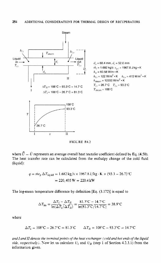
Example 4.2 In a liquid-to-steam two-fluid heat exchanger, the controlling thermal resistance fluid side is the liquid side. Let's assume that the temperature of the steam stays almost constant throughout the exchanger (Tsteam = 108°C) while the liquid changes its temperature from 26.7"C to 93.3"C. The heat transfer coefficient on the steam side is uniform and constant over the heat transfer surface (12,200 W/m2 . K), while on the liquid side, its magnitude changes linearly between 122 W/m2 . K (at the cold end) and 415 W/m2 . K (at the hot end). Determine the heat transfer surface area if the following additional data are available. The mass flow rate of the liquid is 1.682 kg/s. The specific heat at constant pressure of the liquid is 1,967.8 J/kg. K. The heat exchanger is a double-pipe design with the inner tube inside diameter 52.6 mm and the inner tube outside diameter 60.4 mm. The thermal conductivity of the tube wall is 60.58 W/m. K. Assume that no fouling is taking place.
SOLUTION
Problem Data and Schematics: Data for the double-pipe heat exchanger are provided in Fig. E4.2.
Determine: The heat transfer area of the heat exchanger.
Assumpions: All the assumptions described in Section 3.2.1 hold except for a variable heat transfer coefficient on the liquid side. Also assume that there is no thermal entry length effect on U. To apply a conventional design method (say, the MTD method; Section 3.7) a mean value of the overall heat transfer coefficient should be defined (see Section 4.2.3.1).
Analysis: The heat transfer surface area can be calculated from
4 A = - ATl,
254 ADDITIONAL CONSIDERATIONS FOR THERMAL DESIGN OF RECUPERATORS
Steam
Liquid -out
hl,i 1 Tstem Liquid '\
in + Ti,'
.f AT11 = 108°C - 93.3"C = 14.7%
ATI = 108°C - 26.7"C = 81.3"C
do = 60.4 mm, d, = 52.6 rnm
k, = 60.58 Wlm K hLL = 122 Wlm' K h,,,,, = 12200 W/m2 K
Tsteam = 108°C
hi = 1.682 kg/s cP,i = 1967.8 Jlkg K
hbO = 41 5 Wlm' K
Ti,i = 26.7"C = 93.3"C
I I
I I c
I X I1
FIGURE E4.2
where = U represents an average overall heat transfer coefficient defined by Eq. (4.50). The heat transfer rate can be calculated from the entlialpy change of the cold fluid (liquid):
q = "Zcp ATliqui,j = 1.682 kg/s x 1967.8 J/kg. K x (93.3 - 26.7)"C
= 220,435 W = 220.4 kW
The log-mean temperature difference by definition [Eq. (3.172)] is equal to
AT1 -AT,, 813°C - 14.7"C = 38.9"C - A T -
Irn - ln(ATl/ATII) - ln(81.3"C/14.7"C)
where
AT1 = 108°C - 26.7"C = 81.3"C AT11 = 108°C - 93.3"C = 14.7"C
and I and II denote the ternrinalpoints of'the heat exchanger (cold and hot ends of the liquid side, respectively). Now let us calculate U , and UII (step 1 of Section 4.2.3.1) from the information given.
NONUNIFORM OVERALL HEAT TRANSFER COEFFICIENTS 255
1 (52.6 x m) ln(60.4mm/52.6mm) 2 x 60.58 W / m . K + - -
12200W/m2 . K(60.4mm/52.6mm)
-f 1
122 W/m2. K
= (0.7138 + 0.6003 + 81.9672) x m2 . K/W = 83.2813 x m2 . K/W
Therefore,
Ul = 120.1 W/m2 . K
Analogously, UII = 393.6 W/m2 . K by changing 122 W/m2 . K to 415 W/m2 . K in the equation above for l /UI. The magnitude of the local overall heat transfer coefficient at the referent temperature T1iquid,,/2 can be determined using Eq. (4.42), keeping in mind that for a constant specific heat of the fluid, the same form of the equations can be written for both enthalpy and temperature magnitudes:
where
AT?/2 = (AT1 ATlI)'/' = (81.3"C x 14.7"C)1/2 = 34.6"C
Therefore,
34.6"C - 14.7"C Tliquid,l/2 = 93.30c + (26.70c - 93.30c) 8 1 . 3 0 ~ - 1 4 . 7 0 ~ = 73.4"C
and
It is specified that the liquid-side heat transfer coefficient varies linearly from 122 to 415 W/m2 . K with the temperature change from 26.7"C to 93.3"C. Hence from a linear interpolation, hliquid.l/2 at 73.4"C is
hliquid,l/2 = 122 W/m2 ' + (455 (93.3 - 122) - 26.7) c ' (73.4 - 26.7)"C = 327.5 W/m2 . K
Now changing 122 W/m2 . K to 327.5 W/m2 . K in the last term of the l /UI equation above, we get
U1,2 = 314.0 W/m2 . K

256 ADDITIONAL CONSIDERATIONS FOR THERMAL DESIGN OF RECUPERATORS
The apparent overall heat transfer coefficient a t this third point is given by Eq. (4.49) as
34.6"c = 314.0 ~ / m 2 . K u;12 = u,,,% = 314.0 ~ / m 2 . K (m) Finally, the mean overall heat transfer coefficient can be calculated, using Eq. (4.50), as
1 120.1W/m2.K )+'( 3 314.0W/m2 . K )+'( 6 393.6W/m2.K
= 3.934 x lo-' m 2 . K/W
Since the thermal entry length is negligible for liquids and zero for condensing steam, K = 0. Hence,
0 = i7 = 254.2 w / m 2 . K
The heat transfer surface area of the exchanger is now
= 22.29 m2 4 - 220,435 w A = - - AT,, 254.2 W/m2 . K x 38.9K
Discussion and Comments: This simple example illustrates how to determine D and the heat transfer surface area for a counterflow exchanger. For other exchangers, with both fluids as single-phase, the procedure will be more involved, as outlined in Section 4.2.3.1. Calculation of the mean overall heat transfer coefficient by determining the arithmetic mean value of the local values of terminal overall heat transfer coefficients, [i.e., 0 = ( UI + UI1)] will result in this case in a heat transfer surface area about 1 % smaller than the value determined using the elaborate procedure above. It should be noted that the local heat transfer coefficient on the liquid side changes linearly. Often, the changes of heat transfer coefficients are not linear and the values calculated for the mean overall heat transfer coefficient determined using various approaches may be substantially different (Shah and SekuliC, 1998). In those situations, a numerical approach is the most reliable.
4.2.3.2 Numerical Analysis. In the foregoing section, the methodology was presented to take into consideration variations in U due to the temperature effect, the length effect, or both. As mentioned earlier, other factors also play a role in making U non- uniform. In addition, a number of other factors that could violate the assumptions (see Section 3.2.1) are built into the basic E-NTU, P-NTU, or M T D methods, such as nonuniform velocity and temperature distributions at the exchanger inlet, and highly variable fluid properties. All these effects can be taken into account by a numerical analysis.
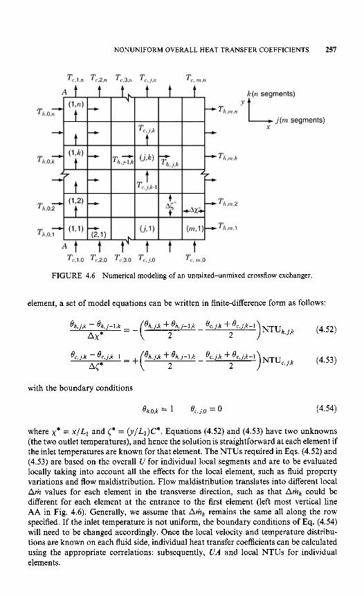
To illustrate the principles, consider an unmixed-unmixed single-pass crossflow exchanger. Divide this exchanger into m x n segments, as shown in Fig. 4.6, with the hot-fluid passage having m segments, the cold-fluid, n segments. The size of individual segments is chosen sufficiently small so that all fluid properties and other variables/ parameters could be considered constant within each segment. Fluid outlet temperatures from each segment are indexed as shown in Fig. 4.6. Energy balance and rate equations for this problem are given in Table 11.2 for an unmixed-unmixed case. For the ( j , k )
NONUNIFORM OVERALL HEAT TRANSFER COEFFICIENTS 257
FIGURE 4.6 Numerical modeling of an unmixed-unmixed crossflow exchanger.
element, a set of model equations can be written in finite-difference form as follows:
with the boundary conditions
eh,O,k = 1 oc , j,O = 0 (4.54)
where x* = x / L I and C* = (y/L2)C*. Equations (4.52) and (4.53) have two unknowns (the two outlet temperatures), and hence the solution is straightforward at each element if the inlet temperatures are known for that element. The NTUs required in Eqs. (4.52) and (4.53) are based on the overall U for individual local segments and are to be evaluated locally taking into account all the effects for the local element, such as fluid property variations and flow maldistribution. Flow maldistribution translates into different local A h values for each element in the transverse direction, such as that Amh could be different for each element at the entrance to the first element (left most vertical line AA in Fig. 4.6). Generally, we assume that Amh remains the same all along the row specified. If the inlet temperature is not uniform, the boundary conditions of Eq. (4.54) will need to be changed accordingly. Once the local velocity and temperature distribu- tions are known on each fluid side, individual heat transfer coefficients can be calculated using the appropriate correlations: subsequently, UA and local NTUs for individual elements.
258 ADDITIONAL CONSIDERATIONS FOR THERMAL DESIGN OF RECUPERATORS
For this particular exchanger, the analysis procedure is straightforward since it repre- sents an explicit marching procedure analysis. Knowing the two inlet temperatures for the element ( l , l ) , two outlet temperatures can be calculated. For the first calculation, all fluid properties can be calculated at the inlet temperature. If warranted, in the next iteration, they can be calculated on each fluid side at the average temperature of the preceding iteration. Once the analysis of the element (1, I ) is completed, analyze element (I, 2) in the same manner since inlet temperatures (Th,o,2 and Tc,l,l) for this element are now known. Continue such analysis for all elements of column 1. At this time, the hot- fluid temperatures at the inlet of the second column are known as well as the cold-fluid outlet temperature from the first column. Continue such analysis to the last column, after which all outlet temperatures are known for both hot and cold fluids.
The example we considered was simple and did not involve any major iteration. If the temperature of one of the fluids is unknown while starting the analysis, the numerical analysis method will become iterative, and perhaps complex, depending on the exchanger configuration, and one needs to resort to more advanced numerical methods. Particularly for shell-and-tube exchangers, not only do the baffles make the geometry much more complicated, but so do the leakage and bypass flows (see Section 4.4.1) in the exchanger. In this case, modeling for evaluating the leakage and bypass flows and their effects on heat transfer analysis needs to be incorporated into the advanced numerical methods.
4.3 ADDITIONAL CONSIDERATIONS FOR EXTENDED SURFACE EXCHANGERS
Extended surfaces or fins are used to increase the surface areat and consequently, to increase the total rate of heat transfer. Both conduction through the fin cross section and convection over the fin surface area take place in and around the fin. Hence, the fin surface temperature is generally lower than the base (primary surface) temperature To if the fin is hotter than the fluid (at T,) to which it is exposed. This in turn reduces the local and average temperature difference between the fin and the fluid for convection heat transfer, and the fin transfers less heat than it would if it were at the base temperature. Similarly, if the heat is convected to the fin from the ambient fluid, the fin surface temperature will be higher than the fin base temperature, which in turn reduces the temperature differences and heat transfer through the fin. Typical temperature distribu- tions for fin cooling and heating are shown in Fig. 4.13. This reduction in the temperature difference is taken into account by the concept of fin efficiency: qJ and extended surface efficiency qo for extended surfaces. Once they are evaluated properly, the thermal resis- tances are evaluated by Eq. (3.24). The heat transfer analysis for direct-transfer type exchangers, presented in Sections 3.2 through 4.2, then applies to the extended surface heat exchangers.
First we obtain the temperature distribution within a fin and the heat transfer through a fin heated (or cooled) a t one end and convectively cooled (or heated) along its surface.
'As mentioned in Section 1.5.3, the heat transfer coefficient for the fins may be higher or lower than for the primary surface, depending on fin type and density. : Kays and London (1998) refer to q, as the fin temperature effectiveness, while lncropera and DeWitt (1996) refer to the fin effectiveness as qc, defined by Eq. (4.156). To avoid possible confusion, we refer to q, as the fin efficiency and qt as the fin effectiveness.

ADDITIONAL CONSIDERATIONS FOR EXTENDED SURFACE EXCHANGERS 259
Next, we derive an expression for fin efficiency. The analysis presented next is valid for both fin cooling and fin heating situations.
4.3.1 Thin Fin Analysis
4.3.1.1 Thermal Circuit and Diyerential Equation. Consider a thin fin of variable thickness 5 as shown in Fig. 4.7. Its length for heat conduction in the x direction (fin height) is t, its perimeter for surface convection is P ( x ) = 2[Lf + S(x) ] and its cross- sectional area for heat conduction at any cross section x is A k ( x ) = 5 ( x ) L f . Note that throughout this section, A k ( x ) will represent the fin cross-sectional area for heat con- duction. Note also that both A/ (the fin surface area for heat transfer) and P can be a function of x (i.e., variable along the fin length a), but they are generally constant with straight fins in heat exchangers so that A/ = P l . The fin is considered thin, if 6 ( x ) << l << Lr. Let us invoke the following assumptions for the analysis.
1.
2.
3. 4. 5. 6 .
I . 8.
There is one-dimensional heat conduction in the fin (i.e., the fin is “thin”) so that the temperature T is a function of x only and does not vary significantly in the y and z directions or across Ak. However, Ak can, in general, depend on x . The heat flow through the fin is steady state, so that the temperature Tat any cross section does not vary with time. There are no heat sources or sinks in the fin. Radiation heat transfer from and to the fin is neglected. The thermal conductivity of the fin material is uniform and constant. The heat transfer coefficient h for the fin surface is uniform over the surface (except at the fin tip in some cases) and constant with time. The temperature of the ambient fluid T, is uniform. The thermal resistance between the fin and the base is negligible.
Temperature difference for convective heat transfer at cross section x
T, = ambient temperature
QO
fin riable
cross section
(4 FIGURE 4.7 Thin
(b) fin of a variable cross section.
260 ADDITIONAL CONSIDERATIONS FOR THERMAL DESIGN OF RECUPERATORS
4 x =
FIGURE 4.8 Energy terms associated with the differential element of the fin.
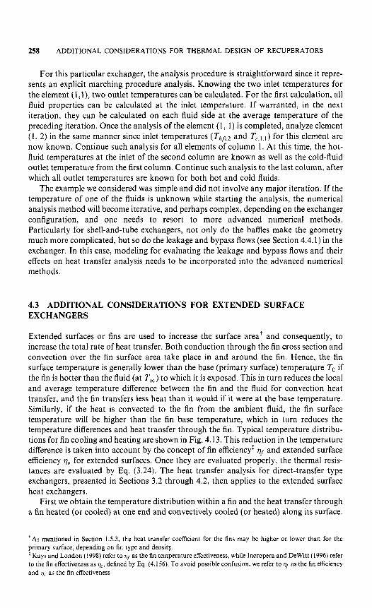
Although two-dimensional conduction exists a t a fin cross section, its effect will be small in most heat exchanger applications. Near the end of Section 4.3.2.2 (p. 285), we discuss what happens if any of assumptions 5 to 8 above are not met.
An energy balance on a typical element between x and x + dx of Fig. 4.7b is shown in Fig. 4.8. Heat enters this element by conduction at x . Part of this heat leaves the cross section at x + dx, and the rest leaves by convection through its surface area dA,f = P d x . The energy balance on this element of length dx over its full width is
The two conduction rate equations associated with conduction through the fin and one convection rate equation for convection to the surroundings for this differential element are given by
(4.56)
(4.57)
dqconv = hdAf ( T - Tm) = h ( P d x ) ( T - T W ) (4.58)
Substituting these rate equations into Eq. (4.55) and simplifying, we get
kf 2 (At:, g) dx = h ( P d x ) ( T - T,)
Carrying out the necessary differentiation and rearranging results in
(4.59)
(4.60)

ADDITIONAL CONSIDERATIONS FOR EXTENDED SURFACE EXCHANGERS 261
or
where
(4.61)
(4.62)
where both P and A k will be functions of x for a variable cross section. Note that m has units of inverse length. To simplify further, define a new dependent variable, excess temperature, as
(4.63)
We assume that the ambient temperature T, is a constant,+ so that d6'ldx = dT/dx and Eq. (4.61) reduces to
d26' d(lnAk,x) d6' 2 -+ _ - m 9 = O dx2 dx dx (4.64)
This second-order, linear, homogeneous ordinary differential equation with nonconstant coefficients is valid for any thin fins of variable cross section. Once the boundary condi- tions and the fin geometry are specified, its solution would provide the temperature distribution, and subsequently, the heat transfer rate through the fin, as discussed later.
4.3.1.2 Thin, Straight Fin of Uniform Rectangular Cross Section. Let us derive specific solutions to Eq. (4.64) for a straight fin of uniform thickness 6 and constant conduction area A k of Fig. 4.9, on page 263. This solution will also be valid for pin fins (having a circular cross section) as long as P and A k are evaluated properly. For the straight fin of Fig. 4.9,
(4.65)
for Lf >> 6. Since Ak,x is constant, d(lnAk,,)/dx = 0, and m2 is constant. Equation (4.64) reduces to
(4.66)
This is a second-order, linear, homogeneous ordinary differential equation. The general solution to this equation is
8 = Cle-mx + C2emx (4.67)
where C1 and C2 (the local nomenclature only), the constants of integration, remain to be established by the boundary conditions discussed in the following subsection.
'If T, is not constant, use Eq. (4.61) for the solution.

262 ADDITIONAL CONSIDERATIONS FOR THERMAL DESIGN OF RECUPERATORS
Boundary Conditions. For a second-order ordinary differential equation [i.e., Eq. (4.66)], we need two boundary conditions to evaluate two constants of integration, C, and C2. The boundary condition at the fin base, x = 0, is simply T = To. Hence,
(4.68)
At the fin tip (x = t), there are five possible boundary conditions, as shown in Fig. 4.10.
CASE 1: LONG, THIN FIN. As shown in Fig. 4 . 1 0 ~ on page 264, the fin is very long compared to its thickness ( t / 6 -+ co), so that T x T , at x = C + cc. Hence,
e(co) = o (4.69)
CASE 2: T H I N F I N W I T H A N ADIABATIC TIP. As shown in Fig. 4.10b on page 264, the fin tip is considered adiabatic and hence the heat transfer rate through the fin tip is zero. Therefore,
or 6) = o .t=r
(4.70)
(4.71)
CASE 3: T H I N FIN W I T H CONVECTIVE BOUNDARY AT THE F I N TIP. As shown in Fig. 4 . 1 0 ~ on page 264, there is a finite heat transfer through the fin tip by convection and hence
Or in terms of 8,
(4.72)
(4.73)
Here we have explicitly specified the fin tip convection coefficient he as different from h for the fin surface. However, in reality, h, is not known in most applications and is considered the same as h (i.e., h, = h).
CASE 4: THIN FIN WITH FINITE HEAT TRANSFER AT THE FIN TIP. AS shown in Fig. 4.10d on page 264, the finite heat transfer through the fin tip is shown as qr since it could be conduction to the neighboring primary surface (not shown in the figure).
(4.74)
or
(4.75)

ADDITIONAL CONSIDERATIONS FOR EXTENDED SURFACE EXCHANGERS 263
FIGURE 4.9 Straight, thin fin of uniform thickness 6.
CASE 5: THIN FIN W I T H FIN T I P TEMPERATURE SPECIFIED. As shown in Fig. 4.10e on page 264, the fin is not very long and the fin tip temperature specified as Tt is constant, so that
et = elxzt = T@ - T, (4.76)
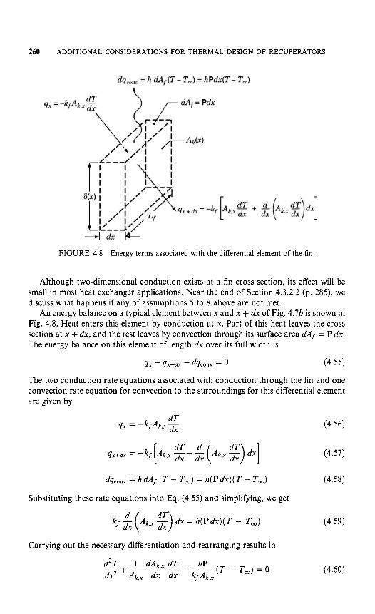
All these boundary conditions are summarized in Table 4.4. In Fig. 4.10, the tem- perature distribution in the fin near the fin tip region is also shown for the first three boundary conditions. The common trend in all three temperature distributions is that the temperature gradient in the fin decreases continuously with increasing x when the fin convects heat to the ambient (T > T,). This is due to less heat available for conduction as x increases because of convection heat transfer from the fin surface. The reverse will be true if the fin receives heat from the ambient. Later we discuss temperature distributions for the last two cases of Fig. 4.10 by Eq. (4.104) and Fig. 4.1 1, respectively.
Total Fin Heat Transfer. The total convective heat transfer from the fin can be found by computing convective heat transfer from the fin surface once the specific temperature distribution within the fin is fmnd from Eq. (4.67) after applying boundary conditions from the preceding section.
The convective heat transfer rate from the differential element dx , from Fig. 4.8, is &cow:
dqconv = h P d x (T - Tm) = h P d x e (4.77)
Hence, the total convective heat transfer rate qconv from the constant cross section fin, excluding the heat exchanged from the tip (to be included later), is found by integrating

264 ADDITIONAL CONSIDERATIONS FOR THERMAL DESIGN OF RECUPERATORS
2- e X- e (4 (el
FIGURE 4.10 Five boundary conditions at x = e for the thin-fin problem: (a) very long fin; (b) adiabatic fin tip, (c) convection at the fin tip; (d) finite heat leakage at the fin tip, (e ) temperature specified at the fin tip.
this equation from x = 0 to x = e.
The conduction heat transfer rate through the base is obtained by
(4.79)
where the temperature gradient (dQ/dx),=o is obtained by evaluating the temperature gradient (dQ/dx) at x = 0 from the specific temperature distribution derived. The heat transfer rate between the fin and the environment a t the fin tip must be equal to the heat transfer rate conducted through the fin a t x = e; it is given by
(4.80)
From the overall energy balance on the fin,
qconv = 40 - 4f (4.81)
From here onward, we consider To > T,, so that qo is coming from the base to the fin (i.e., in the positive x direction) by conduction and q, is leaving fin (again in the positive x direction). For the boundary conditions of Fig. 4.10a and b, qe = 0. Hence
qconv = 90 (4.82)
TABLE 4.4 Boundary Conditions, Temperature Distributions, and Heat Transfer Rates for the Rectangular Profile Thin Fin Problem
Case Fin Tip Condition
Boundary Condition a t x = e
Temperature Distribution in the Fin
Heat Transfer Rate a t x = 0 and e, Temperature
a t x = e, and Fin Efficiency
2
3
Long, thin fin
Thin fin with an adiabatic tip
Thin fin with convection boundary at the fin tip
Thin fin with finite heat transfer at the fin tip
Thin fin with fin tip temperature specified
0 = 8,
0 -coshm(e-x)+Bsinhm(P-x) en coshme+ Bsinhmf? - -
where B = h, mkf
0 en cosh me
cosh m(e - I) - (qlm/hPBn) sinh mx - _
6' - sinhm(P - x) + (B, /Bn) sinhmx en sinh me - -
q , = O B e = O r v = - 1 me
hP hP cosh(2mP) - I m m sinh(2me)
1 tanh me 0, coshme " =me hP sinhme+ Bcoshme m cosh me + B sinh me
yo = -6, tanhme = -80
q p = 0 B.=-
qn =-en
I " = heAk8ncoshml+ Bsinhme
tanh me + B 'v = ( B + d ) ( l + Btanhme)
hP m
qn = -0, tanh me + ye
8, ~ I - (qpm/hPBn) sinhme en cash me - -
hP coshme - ( B , / O n ) =men sinhme
hP coshme - (B0/8,) m sinh me
= -&

266 ADDITIONAL CONSIDERATIONS FOR THERMAL DESIGN OF RECUPERATORS
and the fin heat transfer can be obtained either by integrating the temperature distribu- tion along the fin length [Eq. (4.78)] or by differentiating the temperature distribution and evaluating the derivative at the fin base [Eq. (4.79)]!
For the boundary condition of Fig. 4 . 1 0 ~ and from Eq. (4.81),
40 = qconv + q e (4.83)
If qe is the convection heat transfer from the fin tip, qo represents the total convection heat transfer through the fin surface, including the fin tip.
For the boundary conditions of Fig. 4.10dand e , qe can be positive, zero, or negative, and one needs to apply Eq. (4.81) to determine qconv.
Now let us derive specific temperature distributions for the five boundary conditions.
CASE 1 : LONG THIN F I N (1 /6 + co). Substituting the boundary conditions of Eqs. (4.68) and (4.69) into the general solution of Eq. (4.67), we obtain
CI + c, = 00 (4.84)
c ~ x o + c 2 x c o = o (4.85)
The equality of Eq. (4.85) will hold only if C2 = 0, and hence from Eq. (4.84), Cl = Oo. Thus, the specific solution of Eq. (4.67) has
CI = o o c, = o (4.86)
and
(4.87)
As noted before, the total fin heat transfer rate can be obtained by integrating this temperature profile as indicated by Eq. (4.78) or by differentiating it and using Eq. (4.79), and we get
where m2 = h P / k f A k . For this case,
6'!=0 q e = O (4.89)
CASE 2: T H I N FIN W I T H AN ADIABATIC TIP. Substituting the boundary conditions of Eqs. (4.68) and (4.71) into the general solution, Eq. (4.67), we obtain
CI + c2 = 00 (4.90)
-mC1 ePmL + mCz erne = o (4.91)
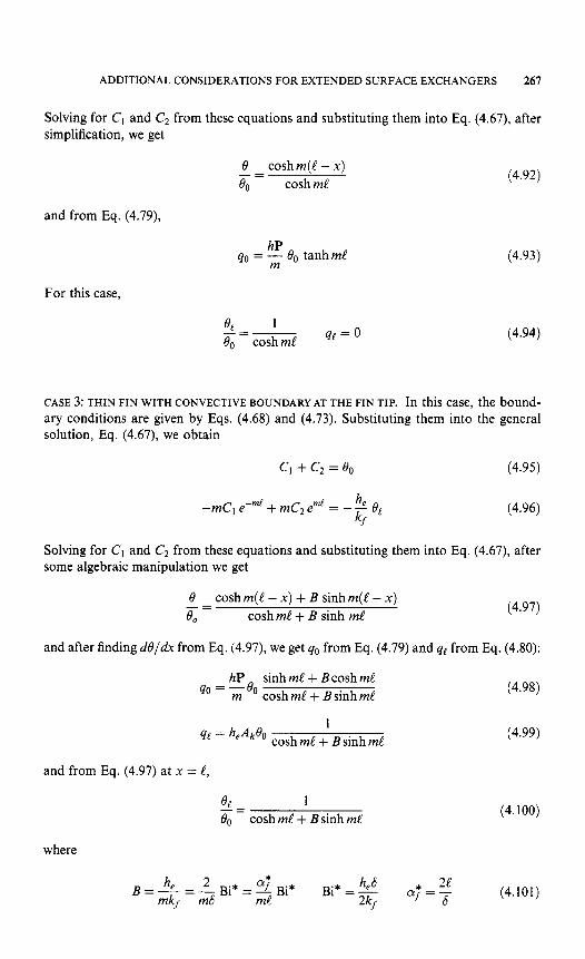
ADDITIONAL CONSIDERATIONS FOR EXTENDED SURFACE EXCHANGERS 267
Solving for CI and C2 from these equations and substituting them into Eq. (4.67), after simplification, we get
and from Eq. (4.79),
For this case.
hP m
qo = - 0, tanhmC
(4.92)
(4.93)
(4.94)
CASE 3: THIN FIN WITH CONVECTIVE BOUNDARY AT THE FIN TIP. In this case, the bound- ary conditions are given by Eqs. (4.68) and (4.73). Substituting them into the general solution, Eq. (4.67), we obtain
c1 + c, = eo (4.95)
(4.96) he k/
-me1 e-me + m e 2 erne = - - ee
Solving for CI and C2 from these equations and substituting them into Eq. (4.67), after some algebraic manipulation we get
(4.97) 0 - coshm(e - x ) + B sinhm(C - x)
60 - _
cosh me + B sinh me
and after finding &/dx from Eq. (4.97), we get qo from Eq. (4.79) and qe from Eq. (4.80):
hP sinhmC + Bcoshme qo = me' cosh me + B sinh me (4.98)
(4.99) 1
4e = heAkeo cosh mC + B sinh mC
and from Eq. (4.97) at x = C,
1 cosh me + B sinh me
- ee Bo -- (4.100)
where

268 ADDITIONAL CONSIDERATIONS FOR THERMAL DESIGN OF RECUPERATORS
Here Bi* is the Biot number at the fin tip; it is the ratio of conduction resistance within the fin [l/{kf/(S/2)}] to convection resistance at the fin tip (l/hc). a; is the fin aspect ratio as defined.
CASE 4: T H I N FIN W I T H FINITE HEAT TRANSFER AT THE F I N TIP. Substituting the boundary conditions of Eqs. (4.68) and (4.75) into the general solution of Eq. (4.67), we get
c, + c, = 00 (4.102)
(4.103)
Solving for C1 and C2 from these equations and substituting them into Eq. (4.67), after some algebraic manipulation, yields
(4.104) 0
00 cash me cosh m(l? - x) - (qpm/hPBo) sinh mx - --
and subsequently, from Eq. (4.79),
(4.105) hP m
qo = - Bo tanh me + q,
and from Eq. (4.80) at x = l?,
Or 1 - (qem/hPBo) sinhme 80 cash me _ - - (4.106)
CASE 5: T H I N FIN W I T H F I N T I P TEMPERATURE SPECIFIED. Substituting the boundary conditions of Eqs. (4.68) and (4.76) into the general solution, Eq. (4.67), we obtain
c, + c, = eo
c l e - m e + c2epne = Be
(4.107)
(4.108)
Solving for CI and C, from these equations and substituting them into Eq. (4.67), after some algebraic manipulation, we get
(4.109) 6 - sinh m(e - x) + (&/e0) sinh mx
00 sinh me - _
Subsequently, the heat transfer rates a t x = 0 and e are obtained for Eqs. (4.79) and (4.80) as
(4.1 10)
(4.1 1 1 ) hP 1 - (er/eo) coshml hP (eo/O,) - coshme --
- m " sinhme 4e = - '0 sinhme m
Next Page