21st uk performance engineering workshop
TRANSCRIPT

School of Computing Science,University of Newcastle upon Tyne
21st UK Performance EngineeringWorkshop
Nigel Thomas
Technical Report Series
CS-TR-916
June 2005
Copyright c©2005 University of Newcastle upon TynePublished by the University of Newcastle upon Tyne,
School of Computing Science, Claremont Tower, Claremont Road,Newcastle upon Tyne, NE1 7RU, UK.

21st UK Performance Engineering Workshop
University of Newcastle
14th/15th July 2005
Edited by Nigel Thomas
ISSN 1368-1060


Contents Preface
1
Keynote Addresses Boudewijn Haverkort
3
Model Checking for Survivability! Jeremy Bradley
5
The Future is Collaborative Performance Engineering Reliability and Security E.Grishikashvili Pereira, R. Pereira, A. Taleb-Bendiab
7
Fault Detection Mechanisms for Autonomic Distributed Applications Christiaan Lamprecht and Aad van Moorsel 11 Performance Measurement of Web Services Security Software Sam St. Clair-Ford, Mohamed Ould-Khaoua, Lewis Mackenzie 21 The Impact of Network Bandwidth on Worm Propagation Stephen A. Jarvis, Guang Tan, Daniel P. Spooner and Graham R. Nudd 31 Constructing Reliable and Efficient Overlays for Peer-to-Peer Live Media Streaming Theory and Practice Richard G. Clegg
43
A Practical Guide to Measuring the Hurst Parameter Paulo Fernandes, Afonso Sales, Thais Webber 57 An Alternative Algorithm to Multiply a Vector by a Kronecker Represented Descriptor
Arpad Tari, Miklos Telek and Peter Buchholz 69 A moment-based estimation method for extreme probabilities Applications 1 R. S. Al-Qassas, M. Ould-Khaoua and L.M. Mackenzie
81
A New End-to-End Traffic-Aware Routing for MANETs Shi Hang Yan, Geyong Min, Irfan Awan 93 Effective Admission and Congestion Control for Interconnection Networks in Cluster Computing Systems
Lan Wang, Geyong Min, Irfan Awan 101Analysis of Active Queue Management under Two Classes of Traffic
S. H. A. Wahab, M. Ould-Khaoua and S. Papanastasiou 111Performance Analysis of the LWQ QoS Model in MANETs
Grid and Web Services Yuhui Chen, Alexander Romanovsky, Peter Li
121
Web Services Dependability and Performance Monitoring James Padgett, Karim Djemame and Peter Dew 125 Predictive Run-time Adaptation for Service Level Agreements on the Grid Andreas Schmietendorf, Reiner R. Dumke, Stanimir Stojanov 137 Performance Aspects in Web Service-based Integration Solutions

Applications 2 Wei Li, Rod Fretwell, Demetres Kouvatsos
153
Performance Distributions of Continuous Time Single Server Queueing Model with Batch Renewal Arrivals: GIG/M/1/N
Saher S Manaseer and M. Ould-Khaoua 159 A New Backoff Algorithm for MAC Protocol in MANETs Burak Simsek, Katinka Wolter and Hakan Coskun 165Analysis of the QBSS Load Element Parameters of 802.11e for a priori Estimation of Service Quality
S. Bani-Mohammad, M. Ould-Khaoua and I. Ababneh 177 Performance Evaluation of Processor Allocation Strategies in the 2-Dimensional Mesh Network
Addendum
E.Grishikashvili Pereira, R. Pereira, A. Taleb-Bendiab
189
Fault Detection Mechanisms for Autonomic Distributed Applications (Full paper)

Preface Welcome to the 21st UK Performance Engineering Workshop, being held for the first time in Newcastle. UKPEW is designed to be a forum for researchers across the UK and beyond to meet and share experiences of their work in the field of performance. The meeting is intended to be approachable to researchers at any stage of their career and is an ideal place to make new contacts and to meet old friends. I very much hope that the 21st UKPEW will be as much of a success in this regard as the previous 20 events. This year the programme consists of eighteen submitted papers across five loosely themed sessions spread over two days. The papers reflect the rise of security, MANETs and web services as important growing concerns for performance engineers, as well as the continued importance of more traditional topics, such as queueing theory. As usual the majority of papers are from the UK, but there are also contributions from Germany, Hungary and Brazil. It is very pleasing to see so many people active in this area in the UK and so many familiar faces returning once more to UKPEW. The level of interest demonstrates a healthy community. I would like to take this opportunity to thank all the authors for preparing their papers professionally and for (almost) sticking to the deadlines. Your hard work made my job much easier. In addition to the regular papers there are also two invited talks, given by Boudewijn Haverkort and Jeremy Bradley. We are delighted to welcome such esteemed researchers to present at UKPEW. Jeremy is an old friend of UKPEW, having been co-chair in Bristol in 1999 and Durham in 2000 and a delegate every year since. He is well known for his work on stochastic process algebra. And will talk about a collaborative environment for performance engineering. Boudewijn is new to the UKPEW forum but is very well known and respected throughout the community. He is currently Professor of Design and Analysis of Communication Systems at the University of Twente and has worked for many years in the area of performance and reliability modelling. Boudewijn will present work undertaken jointly with his PhD student Lucia Cloth on the use of model checking techniques for survivability evaluation. In recent years Newcastle has become one of the pre-eminent cities in the UK, with a reputation for lively night life, modern art and architecture. It is a great place to live and work, and we hope that the UKPEW delegates will find it a great place to visit. If you have time then please make the effort to walk down to the Quayside and over the Millennium Bridge (“The Winking Eye”) to The Sage Gateshead and the Baltic Arts Centre. These buildings have become symbols of the regeneration of this once industrial area of the city and are well worth the walk. I hope you enjoy what Newcastle has to offer and more importantly I hope you enjoy the papers and presentations at UKPEW. If this is your first visit to either Newcastle or UKPEW, I trust that both will impress you enough to want to return. Nigel Thomas (Chair of UKPEW 2005)
1

2

Model Checking for Survivability!
Boudewijn Haverkort and Lucia Cloth
University of Twente, The Netherlands
Abstract Business and social life have become increasingly dependent on large-scale communication and information systems. A partial or complete breakdown as a consequence of natural disasters or purposeful attacks might have severe impacts. Survivability refers to the ability of a system to recover from such disaster circumstances. Evaluating survivability should therefore be an important part of communication and information system design. In this paper we take a model checking approach toward assessing survivability. We use the logic CSL to phrase survivability in a precise manner. The system operation is modelled through a labelled CTMC. Model checking algorithms can then decide automatically whether the system is survivable. We illustrate our method by evaluating the survivability of the Google file system using stochastic Petri nets in combination with CSL model checking.
3

4

The Future is Collaborative Performance Engineering
Jeremy Bradley
Department of Computing, Imperial College London
Abstract Performance engineering is a hard task involving not only a large portion of concurrency theory, but also incorporating stochastic, deterministic and probabilistic concepts of time and choice at the modelling end. More widely performance engineering incorporates the gathering of instrumentation of real systems, the simulation of models of such systems and the real challenge is to have the modelling and simulation results match the performance experiments on the target system. We are working on a performance engineering environment called Perform-db which has at its core the notion that performance engineers need to collaborate in order to maximise the reuse of performance models, analysis, simulations, experiments and structural results. We believe that only in making use of formal modelling results that others have derived or in spotting patterns in experimental data that was produced from other related systems can the overall goal of a performance engineering lifecycle be achieved.
5

6

Fault Detection Mechanisms for Autonomic Distributed Applications. *E.Grishikashvili Pereira, **R. Pereira, **A. Taleb-Bendiab * Department of Computing and IS Edge Hill Uni. College, St. Helen’s Road, Ormskirk, L39 4QP, [email protected] **School of Computing and Mathematical Sciences Liverpool John Moores University, Byrom Street, Liverpool, L3 3AF, UK, [email protected] Abstract: Autonomic computing includes a range of desirable properties, which are best achieved through middleware support. One of these properties is self-healing, the ability that systems may have to reconfigure themselves following the failure of some component. Recently, we have witnessed the development of models to provide middleware-based support for self-healing, service oriented distributed systems. The On-Demand Assembly and Delivery (OSAD) proposed previously by the authors consists of a number of components associated with fault-detection and fault-recovery. In this paper, we consider the performance impact of a number of fault-detection mechanisms, including pre-emptive detection and on-use detection.
Introduction: There is a growing body of knowledge associated with techniques related to self-healing[1-3]. Although to a certain extent self-healing is not yet well defined in terms of scope and architectural models, it has received increased attention lately. A short definition of a self-healing system is a system that is capable of performing a reconfiguration step in order to recover from a permanent fault. The following requirements are likely to be relevant to most self-healing systems: adaptability, dynamicity, awareness, autonomy, robustness, distributability, mobility and traceability. In addition, it is also essential that self-healing systems have strong monitoring abilities. Self-healing properties are particularly useful in dynamic systems, particularly distributed, service oriented systems, where new services may be added and removed from the network, leading to the need for applications to reconfigure themselves [4, 5]. Ideally, such reconfiguration steps would be carried out without user intervention. Distributed service oriented systems provide application developers with the ability to build applications using services provided by other systems across available in a network. Such arrangement requires some form of organisation, normally involving a look up service, which contains information about all services that are available in the network. Applications wishing to use a networked service would carry out a search on the look up service and select, based on some criteria, the service that best matches its requirements. A well-known system based on distributed services is JINI, which provides some support for distributed service-oriented systems [6]. The OSAD model
The On-demand Service Assembly and Delivery (OSAD) model [4] provides an abstract view of the relationship of the distributed components and services. The objective of the OSAD model is to organize the following issues in a uniform framework:
On-demand service delivery and invocation regardless of the location of the service;
7

The automatic assembly of the application in ad-hoc manner based on the user’s requirements;
The ability to self-heal at runtime in terms of replacing a failed component of an application.
Figure 1: the lifecycle of self-healing behaviour in OSAD
One of the tasks of the model is to find distributed components offering specific functionality, that we call offering the service. After the component is found the next task is to make use of this functionality. Finding and assembling components is the role of the Assembly Service:
Assembly Service – this is the core service of the framework and it combines a number of functionalities of the model. Therefore the Assembly service is a combination of different sub-services and modules. It contains:
• A Task Definition service;
• Registration and Discovery Service;
• Service Invocation Service.
Control and monitoring are needed to identify failure, and alert the system to find an alternative replacement for the failed service as the control mechanism should be implemented with self-healing behaviour, in order to improve the newly formed application performance. The control and monitoring are performed by the System Manager. The system manager is responsible for recovering the application from failure. Following failure detection, it notifies the assembly service that a replacement service should be found and selected amongst possible alternatives Fault Detection Mechanisms Failure detection can be implemented in different ways, which can have considerable impact on the performance of the system. Two mechanisms that we put forward for consideration are: Pre-emptive detection and on-use detection. With pre-emptive detection, the service manager checks, on a regular basis, that each of the services associated with the application is alive. If a service fails to respond to the service manager, it is assumed that the service has failed and the recovery process is started and the service manager then notifies the assembly service. With the on-use detection, the service manager monitors locally the service requests and, if a request times-out, it
8
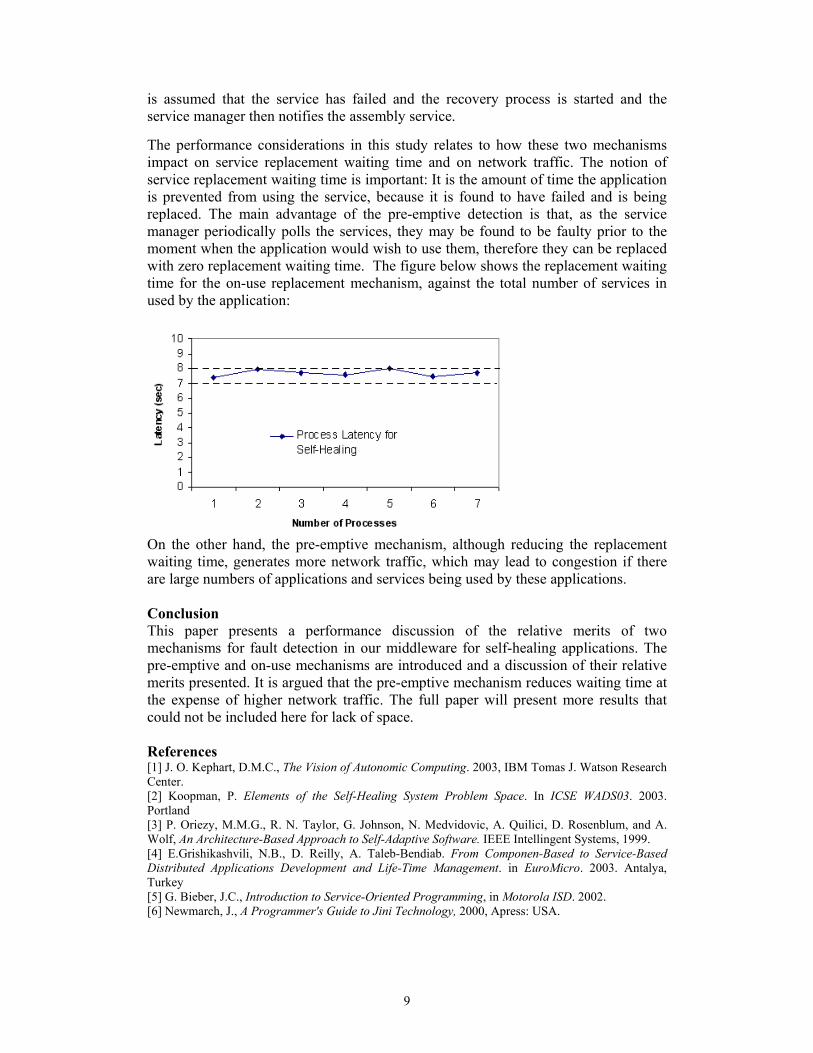
is assumed that the service has failed and the recovery process is started and the service manager then notifies the assembly service. The performance considerations in this study relates to how these two mechanisms impact on service replacement waiting time and on network traffic. The notion of service replacement waiting time is important: It is the amount of time the application is prevented from using the service, because it is found to have failed and is being replaced. The main advantage of the pre-emptive detection is that, as the service manager periodically polls the services, they may be found to be faulty prior to the moment when the application would wish to use them, therefore they can be replaced with zero replacement waiting time. The figure below shows the replacement waiting time for the on-use replacement mechanism, against the total number of services in used by the application:
On the other hand, the pre-emptive mechanism, although reducing the replacement waiting time, generates more network traffic, which may lead to congestion if there are large numbers of applications and services being used by these applications. Conclusion This paper presents a performance discussion of the relative merits of two mechanisms for fault detection in our middleware for self-healing applications. The pre-emptive and on-use mechanisms are introduced and a discussion of their relative merits presented. It is argued that the pre-emptive mechanism reduces waiting time at the expense of higher network traffic. The full paper will present more results that could not be included here for lack of space. References [1] J. O. Kephart, D.M.C., The Vision of Autonomic Computing. 2003, IBM Tomas J. Watson Research Center. [2] Koopman, P. Elements of the Self-Healing System Problem Space. In ICSE WADS03. 2003. Portland [3] P. Oriezy, M.M.G., R. N. Taylor, G. Johnson, N. Medvidovic, A. Quilici, D. Rosenblum, and A. Wolf, An Architecture-Based Approach to Self-Adaptive Software. IEEE Intellingent Systems, 1999. [4] E.Grishikashvili, N.B., D. Reilly, A. Taleb-Bendiab. From Componen-Based to Service-Based Distributed Applications Development and Life-Time Management. in EuroMicro. 2003. Antalya, Turkey [5] G. Bieber, J.C., Introduction to Service-Oriented Programming, in Motorola ISD. 2002. [6] Newmarch, J., A Programmer's Guide to Jini Technology, 2000, Apress: USA.
9

10

Performance Measurement of Web Services Security Software
Christiaan Lamprecht * Aad van Moorsel †
Abstract
Web Services are built on open standards to provide a generic way of communication between heterogeneous environments. Web Service security is an important factor for Web Services to gain increased acceptance. This paper presents how message level security is achieved in web services interactions and in particular explores whether VeriSign’s Trusted Services Integration Kit (TSIK) is a viable option for realising this. Through measurement of TSIK as well as of an implementation using Java Cryptography Extensions (JCE), we conclude that TSIK provides an adequate level of security with minimal additional overheads. However, it would benefit from using SHA-256 in future releases and decreasing algorithm operation time when processing larger messages.
1 Introduction
Web Services have been met with growing interest from academia as well as industry due to its potential to provide a generic global service oriented network which is flexible enough to cater for individual service needs as well as providing increased interoperability between services. For businesses to fully embrace such a new technology they need to be confident that it is secure and can provide them with adequate security features for business interactions [Rat]. Focusing on security at message level, such business interactions typically require: message integrity to ensure messages are unaltered during transit; message confidentiality to ensure message content remain secret; non-repudiation to ensure that the sending party cannot deny sending the received message; and sender authentication to prove sender identity.
This paper will analyse the performance of Web Service security mechanisms. In particular we investigate if VeriSign’s publicly available Trusted Services Integration Kit (TSIK) is a viable security tool with respect to the level of security it provides as well as its efficiency at doing so. We therefore first discuss in section 2 how message integrity, confidentiality, non-repudiation and sender authentication are typically achieved. Section 3 will focus on the level of security provided by TSIK for each of the above. Section 4 will look at asymmetric cryptography in more detail to provide a basis for section 5 which details a comparative evaluation of TSIK’s performance with respect to using the standard Java Cryptography Extensions (JCE). The paper concludes with a summary in section 6. _________________________________________________________________________________
* School of Computing Science, University of Newcastle upon Tyne, [email protected] † School of Computing Science, University of Newcastle upon Tyne, [email protected]
11

2 Message level security
We provide a very brief overview of the well-known techniques available to achieve message integrity, confidentiality, non-repudiation and sender authentication. 2.1 Symmetric cryptography
Symmetric cryptography tries to ensure message confidentiality by encrypting the message (the plaintext) using a secret key to produce an encrypted version of the message (the cipher text), which is then sent instead of the original message. Message integrity is implicitly provided, as altering the cipher text would result in an illegible decrypted message. ‘Symmetric’ refers to the fact that the same secret key is required to decrypt the message on the recipient’s side. Typical symmetric encryption algorithms include DES, Triple DES, RC2, RC5, IDEA and AES. The main problem in this scheme is the key distribution problem; since the same secret key is used to decrypt the message, one must find a way to securely transport the key from sender to recipient. 2.2 Hashing
Hashing tries to ensure message integrity by producing a condensed version of the message, the message digest, which is unique to that message. The hashing algorithm is publicly known and so the recipient can perform the same hash on the received message, to produce another message digest, and compare it to the received digest to asses whether the original message has been altered. Typical hashing algorithms include MD2, MD4, MD5, SHA-1, SHA-256, SHA-384 and SHA-512. Hashing does not provide confidentiality, non-repudiation or authentication. On its own, hashing does not provide message integrity either as both the hash and the message could be replaced by a third party and so prevent the recipient from detecting the attack. Section 2.4 explains how hashing is utilized to ensure message integrity. 2.3 Asymmetric cryptography (public key cryptography)
Asymmetric cryptography provides the same message security guarantees as symmetric cryptography, but additionally provides the non-repudiation guarantee. ‘Asymmetric’ refers to the fact that different keys are used for encryption and decryption. One key is kept secret (‘secret key’) and the other is made public (‘public key’), and are both unique. The recipient’s public key should be used during the encryption process to ensure message confidentiality as only the recipient has the necessary secret key to decrypt the message. If, however, the message is encrypted using the sender’s private key the sender cannot deny sending the message as his private key is unique and is only known to him. Typical asymmetric encryption algorithms include RSA and Elgamal. Asymmetric cryptography is extremely powerful, but this comes at a cost. Especially for longer messages and keys, it is much slower than its symmetric cryptography counterparts [Adams]. 2.4 Experiment Scenario
The results in this paper assume the following typical scenario, in which the above techniques are combined to achieve a more effective security solution through signing, verifying, encryption and decryption. They are combined as follows:
The key, in symmetric cryptography, can be securely transported using public key cryptography by encrypting the symmetric key using the receiver’s public key. The receiver, and only the receiver, can then first decrypt the symmetric key
12

using his private key and then decrypt the message using the decrypted symmetric key. Also note that only the key, which is relatively short, is encrypted using public key cryptography and so reduces encryption overhead.
The message digest, produced by the hash function, can be encrypted using an asymmetric cryptography algorithm to avoid and interception attack. Thus, if the message digest is encrypted using the sender’s private key, only the message can be replaced during transit and not the message digest, since the interceptor does not have the sender’s private key to encrypt the new message digest.
Generating a message digest and then encrypting the message digest using a private key is referred to as signing the message. Decrypting the message digest using the sender’s public key, generating a new message digest of the received message and then comparing the digests is called verifying the message. The performance results of these two techniques, among others, are analysed in this paper.
Sender authentication is achieved when the sender’s public key is signed by a mutually trusted third party. The receiver can then verify the public key as the third party’s public key is trusted. 3 RSA [Ronald]
Understanding the security implications and performance results in sections 4 and 5 requires a deeper understanding of public key cryptography. In particular RSA, which was developed by Ron Rivest, Adi Shamir and Leonard Adleman in 1977 and is used by VeriSign’s TSIK toolkit. We do not explain all the details of RSA, but instead focus on the particular use of RSA in our measurements setup. 3.1 The algorithm [Rivest][Hung]
• Choose 2 large primes p and q such that pq = N • Select 2 integers e and d such that ed = 1 mod )(Nφ
o Where )1)(1()( −−= qpNφ is the Euler totient function of N In general, N is called the Modulus, e the public exponent and d the private exponent. The public key is the pair (N, e) which is made public and the private key is the pair (N, d) which is kept secret. RSA encryption and decryption explained in context of the experiment scenario (section 2.4): Encryption: The symmetric key M:
Encrypted key = Me mod n The message digest M: Encrypted digest = Md mod n Decrypting: The symmetric key C: Decrypted key = Cd mod n The message digest C: Decrypted digest = Ce mod n
13

Where M is the key or digest converted to an integer according to [PKCS#1], C the encrypted key or digest and n the particular modulus, chosen to be either 512, 1024, 2048, 3072 or 4096. In particular, it should be noted that encrypting the key and encrypting the message digest is not the same function as one uses the public- and the other the private exponent.
Therefore, encrypting the symmetric key and decrypting the message digest (in the verification process) is mathematically equivalent as they both use the public exponent. The same can be said for encrypting the message digest (in the signing process) and decrypting the symmetric key as they both use the private exponent.
RSA operation time greatly depends on the length of e and d [Free], such that longer exponents incur much larger time overheads. It would therefore be desirable to use smaller values for e and/or d if possible. 3.2 Smaller public exponent
We consider how the length of the public exponent affects security as both security mechanisms (section 5) exploit this to achieve faster symmetric key encryption and message verification. The smallest value for e is 3 [Dan]. This can however weaken RSA confidentiality assertions. In particular, if e NM < the plaintext can easily be recovered [Rivest]. Also, Hastad’s broadcast attack can be mounted if k cipher texts, encrypted with the same public exponent, can be collected such that k >= e. [Dan]. The Chinese Remainder Theorem (CRT) can then be used to recover the plaintext message [RFC3110] [Dan].
A defense against such attacks would be to ‘pad’ the message using some random bits [Bellare]. Coppersmith imposed further restrictions on this in his “Short Pad Attack” which concludes that for e = 3 an attack can still be mounted, even though a random set of bits are used, if the pad length is less than 1/9th of the message length [Dan].
PKCS#1 [RFC3447] [PKCS#1] does however propose the use of Optimal Asymmetric Encryption Padding (OAEP) [Bellare] for new applications and PKCS1-v1_5 for backward compatibility with existing applications. Although e = 3 can provide adequate security, if necessary precautions are taken, the current recommendation is e = 216 + 1 [Dan] which is still small, requiring only 17 multiplications, but big enough to solve the above problems at the cost of a slight increase in encryption time.
Short public exponents are not however a concern for signature schemes [RFC3110][Rivest]. 3.3 Smaller private exponent
A shorter private exponent would result in faster key decryption and message signing. Typically the private exponent is the same length as the modulus regardless of the public exponent length. M. Wiener [Wiener] has however shown that if d < ⅓N0.24 the private exponent can be obtained from the public key (N, e). Since N is typically 1024 bits long, d must be at least 256 bits long. More recently, Boneh and Durfree have shown this to be closer to d < N0.292 [Durfee] [Hung] and predicted the likely final result to be closer to d < N0.5 [Dan][Durfee].
Other techniques used to decrease algorithm operation time include the use of the Chinese Remainder Theorem [Dan], know as RSA-CRT, which is said to be
14
approximately 4 times faster than using standard RSA algorithms [Hung]. Rebalanced RSA-CRT can also be used and tries to shift the cost towards the usage of the public exponent e [Shacham] [Wiener]. 4 Security software analysis
Java keytool, Java’s Key and Certificate Management Tool, is used to create the Java keystore, with appropriate key pairs, used by TSIK and JCE. The keytool generates key pairs where N is user specified (512, 1024 or 2048), d is the same length as N and e defaults to 216 + 1 (i.e. 17 bits long). As stated in section 3.2 and 3.3, these values are adequate and it is currently recommended that the user selects the modulus to be at least 1024 bits.
TSIK 1.10 provides additional functionality, above that of the Java Cryptography Extensions (JCE), to construct valid XML messages after encryption/decryption or signing/verifying. These messages conform to the W3C XML Signature and Encryption specifications [xmldsig] [xmlenc]. TSIK supports Triple DES (in Cipher Bite Chaining mode) for symmetric encryption, as defined by W3C [tdes]. Using a key length of at least 112 bits will currently provide sufficient security. Triple DES is however relatively slow compared to other more recent contenders such as AES [Junaid]. Conversely, it has stood the test of time and so is potentially a more reliable solution.
Only SHA-1 is provided for message digest generation (Digest length of 160 bits). SHA-1 has very recently been shown to be less secure than predicted and it is recommended that SHA-256 or above should be used [sha]. RSAES-PKCS1-v1_5 algorithm, specified by W3C [rsa15] and [RFC2437], is used as the RSA standard. As stated in section 3.2 above; if backward compatibility is not an issue OAEP should be used in preference to PKCS1-v1_5. However, PKCS1-v1_5 provides adequate security assuming the programmer is aware of certain issues. Also, [RFC2437] indicates that RSA-CRT is used.
JCE does not support the creation of valid XML messages but supports various symmetric key algorithms including AES, Triple DES and RC5. It also supports SHA-1, SHA-256, SHA-512 and MD5, amongst others, for message digest generation. It also specifies that the padding is applied according to [PKCS#1]. RSA-CRT is also used. 5 Performance analysis
The following section details a comparative evaluation of the performance of VeriSign’s TSIK toolkit with respect to the standard Java Cryptography Extensions (JCE) in order to identify whether TSIK is a viable tool to secure web service transactions. 5.1 Environment
All experiments were run on a 3GHz Intel Pentium 4 with 1GB RAM, running Java(TM) 2 Runtime Environment, Standard Edition (build 1.4.2-b28) on top of Linux Fedora Core 2. We used Bouncycastle [bounce] as the Java RSA provider for both JCE and TSIK, and used Apache Axis 1.2 to generate the appropriate WSDL interface for the web service, which was hosted on Tomcat 5. Axis was used to both generate the appropriate SOAP messages, from the java code and TSIK XML documents, to be sent to the web service, also know as the server, and also generate
15

the SOAP messages to be sent back from the web service to the client. We took performance measurements on the client and server side where the TSIK and JCE implementations reside. Message transmission and conversion delays were not measured. 5.2 Experiments
We set up three experiments, as detailed below. Experiment 1:
In experiment 1 we analyse the performance of Triple DES, as function of message size:
• Client side: Message plaintext encrypted using Triple DES with a keysize of 168. Symmetric key encrypted using an RSA public key (Modulus 1024)
• Server side: Encrypted symmetric key decrypted using RSA private key (bit length 1024) and cipher text then decrypted.
Experiment 2:
In experiment 2 we analyse the combined performance of SHA-1 and RSA algorithms, as a function of the message size:
• Client side: Message signed using SHA-1 and RSA private key (bit length 1024)
• Server side: Message verified using SHA-1 and RSA public key Experiment 3:
In experiment 3 we analyse how the modulus size affects the performance of RSA during signature creation and verification:
• Client side: Message signed (as in experiment 2) using RSA key sizes 512, 1024 and 2048.
• Server side: Message verified. 5.3 Results
We executed above experiments for TSIK as well as JCE. We repeated the first two experiments for messages with a range of plaintext sizes, namely 2, 4, 8, 16, … , 512 and 1024 kB. Experiment 3 was done using a 2 kB plaintext size. The results are shown in the graphs below. It should be noted that all points on graphs 1 and 3 exhibit confidence intervals of 3 milliseconds and points on graphs 2 and 4 exhibit confidence intervals of 0.1 milliseconds. Both with probability 0.9 (Where 1.0 is certain).
16

248163264
128
256
512
1024
2481632 64128
256
512
1024
2481632 64128
256
512
1024
2481632 64128
256
512
1024
0
100
200
300
400
500
600
700
8002 33 62 93 123
154
184
215
246
276
307
337
368
399
427
458
488
519
549
580
611
641
672
702
733
764
792
823
853
884
914
945
976
1006
Data size (kB)
Tim
e (m
s)
Encrypt TSIKDecrypt TSIKEncrypt JCEDecrypt JCE
Figure 1: Triple DES encryption time
2481632 64 128 256 512 1024
2481632 64 128 256 512 1024
2481632
64 128 256 512 1024
2481632 64 128 256 512 1024
0
2
4
6
8
10
12
14
2 33 62 93 123
154
184
215
246
276
307
337
368
399
427
458
488
519
549
580
611
641
672
702
733
764
792
823
853
884
914
945
976
1006
Data (kB)
Tim
e (m
s)
Encrypt TSIKDecrypt TSIKEncrypt JCEDecrypt JCE
Figure 2: RSA-1024 encryption time of 168 bit Triple DES key
17
Experiment 1
Figure 1 shows that JCE performs noticeably better for large file sizes. It also shows that Triple DES encryption takes longer than decryption in both cases (TSIK and JCE). Note that the graph also indicates that for very large messages it is decryption that takes longer when using TSIK. We have no explanation for this, and suspect it has to do with the particulars of the implementation.
For RSA we see the opposite effect. Figure 2 indicates that RSA encryption takes less time than decryption. As we hinted at earlier in this paper, that is caused by the size of the keys used in encryption and decryption. For encryption, the public key is used, which has a small public exponent of 17 bits. When comparing TSIK with JCE, we see that the differences are minimal. Decryption varies by an average of about 1 millisecond between the implementations and encryption even less.
248163264
128
256
512
1024
2481632 64128
256
512
1024
2481632 64 128256
512 1024
2481632 64 128256
512
1024
0
20
40
60
80
100
120
140
160
180
2 33 62 93 123
154
184
215
246
276
307
337
368
399
427
458
488
519
549
580
611
641
672
702
733
764
792
823
853
884
914
945
976
1006
Data (kB)
Tim
e (m
s)
Sign TSIKVerify TSIKSign JCEVerify JCE
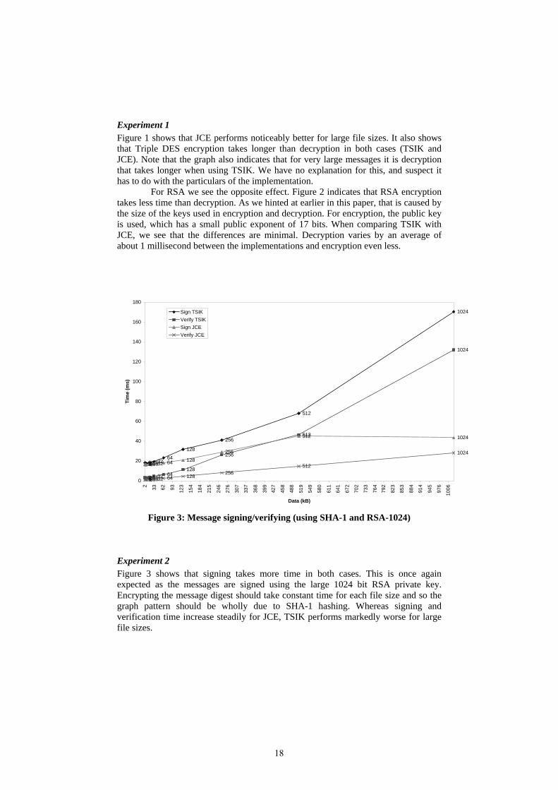
Figure 3: Message signing/verifying (using SHA-1 and RSA-1024)
Experiment 2
Figure 3 shows that signing takes more time in both cases. This is once again expected as the messages are signed using the large 1024 bit RSA private key. Encrypting the message digest should take constant time for each file size and so the graph pattern should be wholly due to SHA-1 hashing. Whereas signing and verification time increase steadily for JCE, TSIK performs markedly worse for large file sizes.
18
0
20
40
60
80
100
120
512 1024 2048
Public keysize (bits)
Tim
e (m
s)
Sign TSIK
Sign JCE
Verify TSIK
Verify JCE
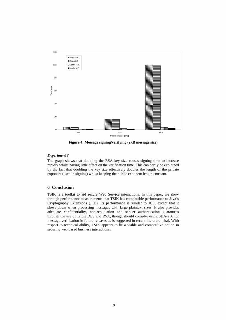
Figure 4: Message signing/verifying (2kB message size)
Experiment 3
The graph shows that doubling the RSA key size causes signing time to increase rapidly whilst having little effect on the verification time. This can partly be explained by the fact that doubling the key size effectively doubles the length of the private exponent (used in signing) whilst keeping the public exponent length constant. 6 Conclusion
TSIK is a toolkit to aid secure Web Service interactions. In this paper, we show through performance measurements that TSIK has comparable performance to Java’s Cryptography Extensions (JCE). Its performance is similar to JCE, except that it slows down when processing messages with large plaintext sizes. It also provides adequate confidentiality, non-repudiation and sender authentication guarantees through the use of Triple DES and RSA, though should consider using SHA-256 for message verification in future releases as is suggested in recent literature [sha]. With respect to technical ability, TSIK appears to be a viable and competitive option in securing web based business interactions.
19
7 References
[Rat] Jason. Bloomberg, Testing Web Services Today and Tomorrow, Rational Edge, October 2002.
[Free] William Freeman and Ethan Miller, “An Experimental analysis of cryptographic overhead in performance-critical systems”, MASCOTS, October 1999.
[Adams] Carlistle Adams and Steve Lloyed, Understanding PKI second edition, Addison-Wesley 2003 p14.
[Ronald] Ronald L. Rivest, Adi Shamir, and Leonard M. Adleman. “A method for obtaining digital signatures and public-key cryptosystems,” Communications of the ACM, 21(2):120-126, 1978.
[Rivest] Ronald L. Rivest and Burt Kaliski, RSA problem, December 10, 2003.
[Hung] Hung-Min Sun and Mu-En Wu, An approach towards Rebalanced RSA-CRT with short public exponent.
[PKCS#1] RSA Laboratories, PKCS#1 v2.1: RSA Cryptography Standard, June 14, 2002.
[Dan] Dan Boneh, Twenty Years of attacks on the RSA cryptosystem. [RFC3110] D. Eastlake, “RSA/SHA-1 SIGs and RSA KEYs in the Domain
Name System (DNS),” IETF Network Working Group, RFC 3110, May 2001.
[Bellare] M. Bellare and P. Rogaway. “Optimal asymmetric encryption,” In EUROCRYPT ’94, Lecture Notes in Computer Science volume 950, pages 92-111. Springer-Verlag, 1994.
[RFC3447] J. Jonsson and B. Kaliski, “Public-Key Cryptography Standards (PKCS) #1: RSA Cryptography, Specifications Version 2.1,” IETF Network Working Group, RFC 3447, February 2003.
[Wiener] M. Wiener. “Cryptanalysis of short RSA secret exponents,” IEEE Transactions on Information Theory, 36:553-558, May 1990.
[Durfee] D. Boneh and G. Durfee. “Cryptanalysis of RSA with private key d less than N0.292,” IEEE Transactions on Information Theory, 46(4):1339-1349, July 2000.
[Shacham] D. Boneh and H. Shacham, “Fast Variants of RSA,” CryptoBytes, 2002, Vol. 5, No. 1, Springer, 2002.
[xmldsig] http://www.w3.org/2000/09/xmldsig# [xmlenc] W3C Recommendation, XML Encryption Syntax and Processing,
http://www.w3.org/TR/xmlenc-core, 10 December 2002. [tdes] http://www.w3.org/2001/04/xmlenc#tripledes-cbc [Junaid] Junaid Aslam, Saad Rafique and S. Tauseef-ur-Rehman, “Analysis
of Real-time Transport Protocol Security,” Information Technology Journal 3 (3):311-314, 2004.
[sha] Arjen K. Lenstra, Further progress in hashing cryptanalysis, February 26, 2005.
[rsa15] http://www.w3.org/2001/04/xmlenc#rsa-1_5 [RFC2437] B. Kaliski and J. Staddon, “PKCS #1: RSA Cryptography
Specifications Version 2.0,” IETF Network Working Group, RFC 2437, October 1998.
[bounce] http://www.bouncycastle.org
20
The Impact of Network Bandwidth on Worm Propagation
Sam St. Clair-Ford, Mohamed Ould-Khaoua, Lewis Mackenzie
Department of Computer Science University of Glasgow
Glasgow G12 8RZ UK
Abstract- This paper evaluates the performance impact that real world ratios of different machine connection speeds has on worm propagation through a computer network. The impact is analysed on three different topologies, notably scale free, small world and random networks, to assess whether results are specific to a particular topology or taking bandwidth into account has an overall effect regardless of the topology in question.
I. INTRODUCTION
The propagation speeds and the size of the infection base for viruses and worms to infect has increased dramatically over the years. From the Melissa virus in 1999 to the SQL Slammer worm in 2003 through to the MyDoom worm and its variants in 2004, machines connected to the Internet have been barraged with threats which could have an impact on a global scale. If an attacker could infect and gain control of a large number of machines then the damage they can do is immense, from ordering Distributed Denial of Service attacks on specific sites to harvesting confidential data and credit card information. Also they can sow misinformation from user’s machines and have a major role in provoking warfare between nations and servicing terrorism across the world [1]. Research into simulating worm propagation and devising new ways of counteracting their spread has focused chiefly on the spread of warnings, [2-4] the detection and filtering of “malicious” traffic [3-6] and the inoculation of specific nodes to slow or stop the spread of infection [7-8]. However these studies have focused on the network at an abstract level to simplify network complexities. One of the main complexities that is missing is that of bandwidth capacity that each node is able to send and receive both worms and warnings. This paper will show that considering the bandwidth factor has a great impact on the outcome of any performance analysis. The authors in [1] have introduced two theoretical worms, “Warhol” and “flash” worm, which could potentially infect every vulnerable machine in a few minutes or as a little as 30 seconds for flash worms. The limiting factor that restricts these worms is the bandwidth that an infected machine can send out copies of itself [9] and as such taking this parameter out of simulations will have an impact on being able to test new strategies against these potential worms. CodeRed (crV2), the first worm to reach over 90% of vulnerable hosts in less than 14 hours [10] has been taken by much of the literature as being the benchmark to test new strategies against. However as the SQL Slammer or Sapphire worm showed in early 2003 that CodeRed is by no means the worst that could be unleashed on the internet. The SQL Slammer worm was the fastest spreading worm in history doubling in population size every 8.5 seconds, and showed the world what potential damage a
21

malicious worm could do. One of the key differences between the two worms was that while Code Red was TCP based, in other words having to establish a connection with its destination, SQL Slammer was UDP based, needing no acknowledgement what so ever. On this principle it could invoke a fire and forget principle and could send out packets as fast as the particular channel could allow. In other words the SQL Slammer worm limiting factor was bandwidth based, restricted only by the connection speed of the infected host. Code Red on the other hand, was latency based, having to wait for a connection to be established before infecting the target host. The SQL slammer worm therefore is a much closer approximation of what the worst case worms of [1] might look like and as a consequence this research looks into simulating such devastating worms that are only limited by bandwidth and seeing if previous models and solutions withstand such attacks.
II. BACKGROUND
In order to delay or prevent the spread of malicious viruses and worms there are three main areas that have been examined as possible strategies. Firstly the technique of intrusion detection where either machines or the network links themselves are monitored for potential threats. This is known as host based and network based intrusion detection for machine monitoring and network monitoring respectively. [3, 5, 6] have all highlighted the main drawback of these techniques, namely that of having a centralized detection system which handles all the monitoring for the network. Having this setup presents a single point of failure, that if exploited could turn the whole defence system against itself [11]. Another problem that intrusion detection techniques face is that of differentiating the malicious from regular traffic. These again fall into two main categories, anomaly and rule based detection. Rule based detection systems, as the name implies make decisions based on matching scenarios to a set of rules. Rules such as rejecting all packets from a particular source can be very effective if the rule set is well designed; however the system does have the weakness that it can’t cope with attacks that it doesn’t have a rule to deal with. Attacks that are novel and not expected will break such systems as the defences are not attuned to dealing with them. To address this issue the alternative method of anomaly detection establishes a definition of what is normal traffic and anything outside this is deemed dangerous and in need of investigation. The natural problem that occurs of course is that of defining what is normal. Users may suddenly decide to use the network in a way that is different than normal or not expected and thus many false positives or false alarms may be raised. On the flip side, an attacker can work to the borderline of what is deemed normal slowing expanding this definition, if it is dynamically created, until creating an exploit is considered normal by the system. An alternative to intrusion detection is that of broadcasting warning to machines to tell them to look out for a new attack, similar in principle to the media alerting the public to a particular threat. Following through with this analogy both situations are confronted with the same problem of how much to trust an information source. Furthermore there is the difficulty of warning potential targets faster than the worm can propagate [4].
22

The Indra project, [3] established in 2003 is a peer-to-peer based intrusion detection system that warns other peers when it detects dangerous traffic. Also following a similar peer-to-peer based system [2, 7] are designed to have peers encourage other nodes it considers to be friends to increase their defences in the case of an attack. With regards to automated attacks such as viruses and worms the principle behind both these systems is the ability to find and compromise new hosts in order survive and propagate. Common methods to do this are email based propagation that rely on sending copies of a virus to email addresses found on a new victims machine, or exploit based propagation that rely on attacking a particular fault in a given application or operating system. Depending on the exploit further propagation can be made by either randomly scanning IP addresses until targets are found by chance or by having a pre-built list of vulnerable IP addresses which can be attacked [1]. In turn this list of vulnerable hosts can be generated by either doing the random scanning before the attack is launched, or by making use of the actual exploit. For example, if the exploit were in an application that is designed for network communication, such as a file sharing application or instant messenger then, assuming a significant portion of the users of this system use the same application to interact with each other, a network of vulnerable machines is already available to the attacking program. As different infections can clearly use different methods of distribution, each of these methods can be regarded in terms of how their targets are connected. As with all networks, each one follows a particular topology, be it scale-free, random, lattice and so on, and as such, defences can be designed to exploit characteristics of these topologies. In their paper [8] Pastor-Satorras and Vispignani have explored immunization strategies for scale-free networks, focusing on immunizing specific highly connected nodes in order to quarantine an infection to a small section of the network. Each of these defence techniques defines their relative results in terms of the fraction of nodes that were saved from infection and uses parameters such as propagation speed to define different kinds of infections. As well as this common theme of measurement they also have a common theme of expecting each node to behave in a similar manner, warning or infecting at the same speed. This research shows that if nodes have variable bandwidth then there is a large difference in the propagation rate of the worm.
III. SYSTEM MODEL
This section describes real world scenarios and relates these scenarios to properties that the simulator will try to emulate and adjust. While it will relate to specific examples the simulator was designed to replicate properties of the scenario not just the particular scenario in question. In order to examine the propagation of bandwidth limited worms the first consideration was to define what types of machines such worms will be targeted at. To emphasise this is a cross section of three different classes of machines were considered, from home systems running on dial up connections to broadband connections and finally high-speed university campus connections. The ratios for how these three classes of connection were divided up were taken from [13] by David Alderson where he describes that the distribution in connection speeds world wide is divided into these three main categories. These ratios are divided 50% 20% and 30% of internet users for the dial up, broad band and campus connections respectively.
23

Each of these nodes could be used for different purposes, from simple emailing to high bandwidth file sharing. In order to accommodate this, the bandwidth distribution was done two different ways; firstly connectivity based where high bandwidth capacities were allocated on a highest number of links first. To clarify, using the ratios described, the top 30% most connected nodes are allocated the campus speed connection, the next 20% are allocated the broadband connection and the remainder are left with dialup speeds. This method was selected to emulate a file-sharing network with high capacity nodes acting as hubs and taking up the slack of lower capacity nodes. The second distribution method was that of random allocation, in order to replicate a network defined by email or instant messenger links. Logically connectivity should have no bearing on bandwidth load as a user’s email ties can be accessed from different machines and therefore from potentially different connection speeds. In examining different topologies, in order to justify confining a worm to follow a particular topology instead of just moving to any node it could successfully probe, this research assumes that the worm is designed with speed as a priority and as such will try to exploit any means necessary to reduce wasted scanning of large address spaces. In order to do this, the worm could use a number of strategies such as having a pre-built list of nodes that it can infect, or it could exploit a systems connection structure itself. Such exploits could be using email addresses stored on a machine, or peers that a file sharing program is currently connected to. This therefore confines the worm to following the topology that email contacts or file-sharing networks follow, giving this research its different topologies to examine. The SQL Slammer worm propagates by using up all the available bandwidth. While the worm propagates from a particular machine all normal background traffic from that machine is prevented from reaching the network. Other machines which are not transmitting the worm still respond with the portion of their available bandwidth capacity not used by their background traffic
IV. SIMULATION MODEL
This section describes the design of the simulation model, the input parameters and metrics used in the performance analysis. Below are two tables that summarise the input and output parameters that have been used. TABLE 1: INPUT PARAMETERS TABLE 2: OUTPUT PARAMETERS
Name Range/Value Name Range/Value Nodes 106 Infected Nodes 0-106 Iterations 5,000 Simulation Time 0-20,000 Simulation Time 20,000 Topology Scale-Free Small-World
Random
Bandwidth 255,1,25,500 Bandwidth Distribution
Uniform, Connectivity based random
24
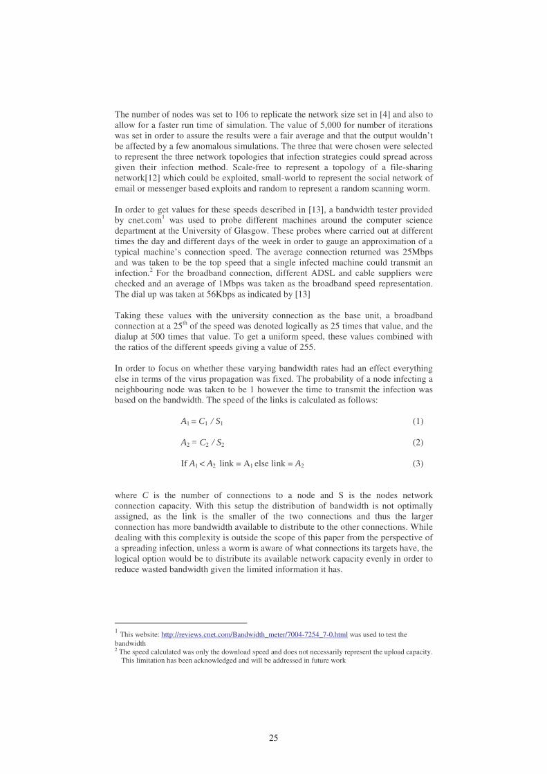
The number of nodes was set to 106 to replicate the network size set in [4] and also to allow for a faster run time of simulation. The value of 5,000 for number of iterations was set in order to assure the results were a fair average and that the output wouldn’t be affected by a few anomalous simulations. The three that were chosen were selected to represent the three network topologies that infection strategies could spread across given their infection method. Scale-free to represent a topology of a file-sharing network[12] which could be exploited, small-world to represent the social network of email or messenger based exploits and random to represent a random scanning worm. In order to get values for these speeds described in [13], a bandwidth tester provided by cnet.com1 was used to probe different machines around the computer science department at the University of Glasgow. These probes where carried out at different times the day and different days of the week in order to gauge an approximation of a typical machine’s connection speed. The average connection returned was 25Mbps and was taken to be the top speed that a single infected machine could transmit an infection.2 For the broadband connection, different ADSL and cable suppliers were checked and an average of 1Mbps was taken as the broadband speed representation. The dial up was taken at 56Kbps as indicated by [13] Taking these values with the university connection as the base unit, a broadband connection at a 25th of the speed was denoted logically as 25 times that value, and the dialup at 500 times that value. To get a uniform speed, these values combined with the ratios of the different speeds giving a value of 255. In order to focus on whether these varying bandwidth rates had an effect everything else in terms of the virus propagation was fixed. The probability of a node infecting a neighbouring node was taken to be 1 however the time to transmit the infection was based on the bandwidth. The speed of the links is calculated as follows: A1 = C1 / S1 (1)
A2 = C2 / S2 (2) If A1 < A2 link = A1 else link = A2 (3)
where C is the number of connections to a node and S is the nodes network connection capacity. With this setup the distribution of bandwidth is not optimally assigned, as the link is the smaller of the two connections and thus the larger connection has more bandwidth available to distribute to the other connections. While dealing with this complexity is outside the scope of this paper from the perspective of a spreading infection, unless a worm is aware of what connections its targets have, the logical option would be to distribute its available network capacity evenly in order to reduce wasted bandwidth given the limited information it has.
1 This website: http://reviews.cnet.com/Bandwidth_meter/7004-7254_7-0.html was used to test the bandwidth 2 The speed calculated was only the download speed and does not necessarily represent the upload capacity.
This limitation has been acknowledged and will be addressed in future work
25
B. ASSUMPTIONS
• Probability of a targeted node being infected is 1 • No defensive strategies such as immunization or warnings allowed • Random node and link failure or node recovery is removed from the
simulator The reason for a probability of 1 is that this simulator defines a worst case scenario where it is the bandwidth of a node that decides how soon a neighbouring node becomes infected. Relating this to a real world situation, the infected source node sends out copies to a limited set of known targets and as such sends copy after copy until the target node is infected. As this is the worst case scenario then the first copy of the worm always reaches its destination representing a probability of 1. The reason for removing node failure and node recovery from the simulator is two fold. Firstly, as this is simulating a fast spreading worm, or a worm that travels faster than human intervention could occur, then a node cannot recover within the simulation time window; i.e. the length of time it takes for all nodes to become infected. With regards to node and link failure, a link or node failure from a spreading worm’s perspective would be equivalent to an immunization defensive strategy and therefore would not constitute a worst case scenario.
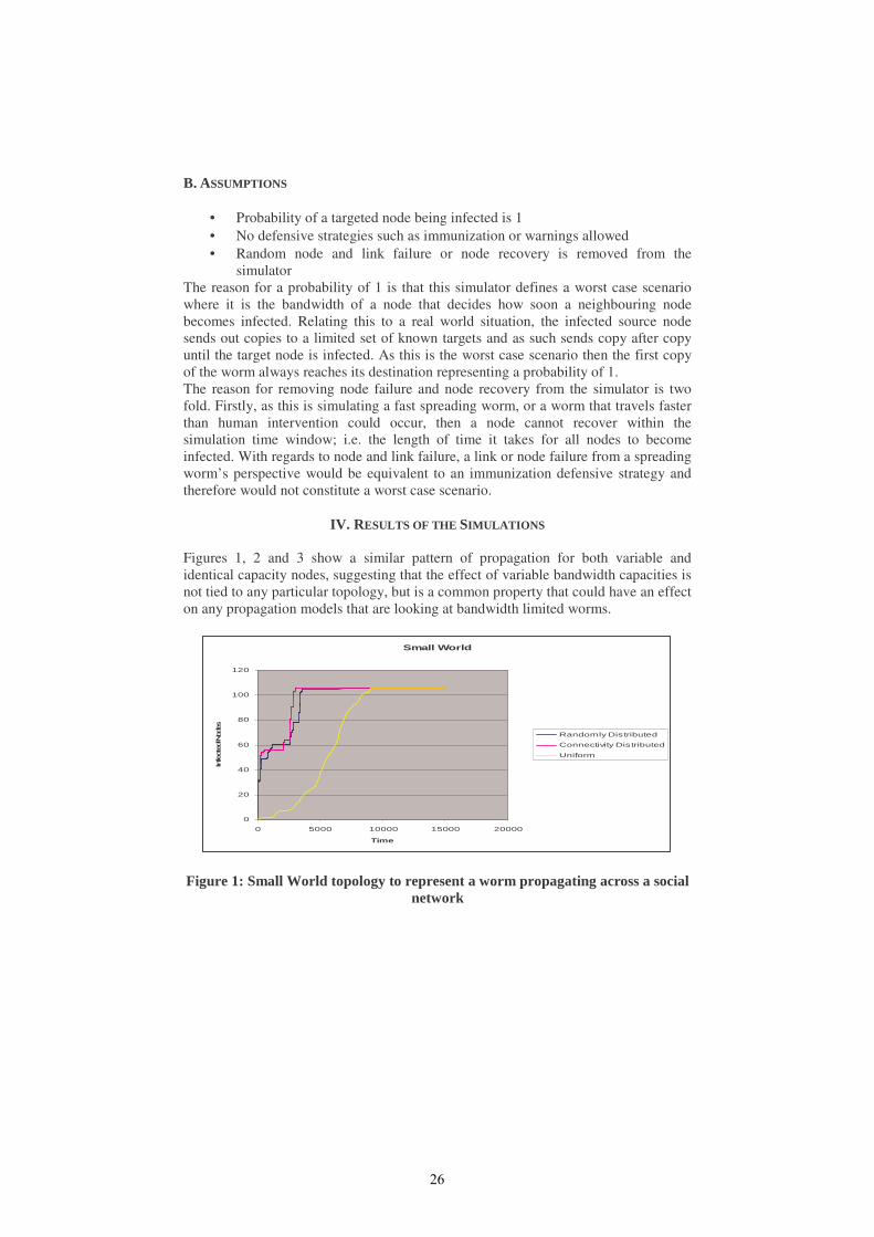
IV. RESULTS OF THE SIMULATIONS Figures 1, 2 and 3 show a similar pattern of propagation for both variable and identical capacity nodes, suggesting that the effect of variable bandwidth capacities is not tied to any particular topology, but is a common property that could have an effect on any propagation models that are looking at bandwidth limited worms.
Small World
0
20
40
60
80
100
120
0 5000 10000 15000 20000
Time
Infe
cted
Nod
es
Randomly Distributed
Connectivity Distributed
Uniform
Figure 1: Small World topology to represent a worm propagating across a social network
26
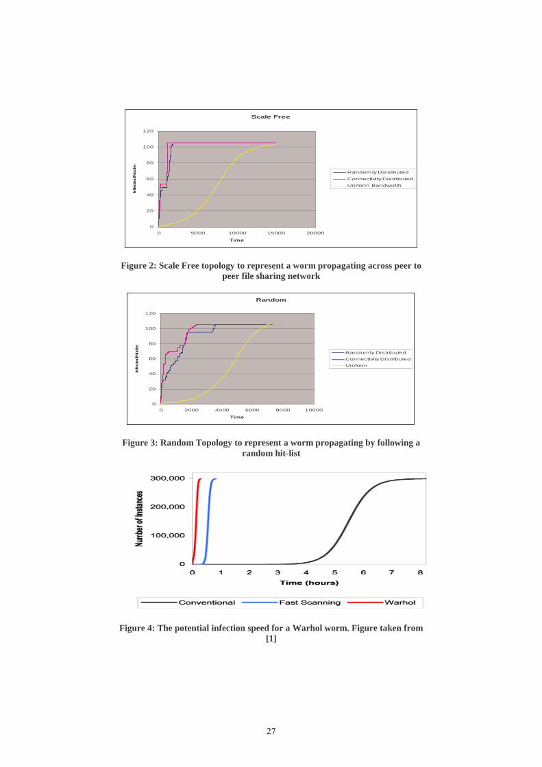
Scale Free
0
20
40
60
80
100
120
0 5000 10000 15000 20000
Time
Infe
cte
d Nod
es
Randomly Distributed
Connectivity Distributed
Uniform Bandwidth
Figure 2: Scale Free topology to represent a worm propagating across peer to peer file sharing network
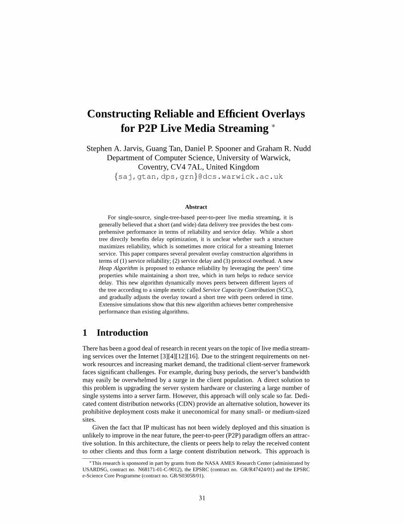
Random
0
20
40
60
80
100
120
0 2000 4000 6000 8000 10000
Time
Infe
cte
d Node
s
Randomly Distributed
Connectivity Distributed
Uniform
Figure 3: Random Topology to represent a worm propagating by following a random hit-list
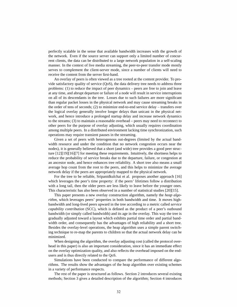
Figure 4: The potential infection speed for a Warhol worm. Figure taken from [1]
27

As can been seen on any of the figures, the propagation speed is much more severe for variable node bandwidth as there is the possibility of finding a few fast routes through the network due to the wide range of different possible connection speeds. While 50% of all the nodes are almost twice as slow for the variable bandwidth as they are for the uniform speed network there are a few high speed nodes that the simulators results show can more than make up for this weakness. While the uniform bandwidth simulations follow that of a sigmoid function, trailing off as they near complete infection of the network, the variable bandwidth graph goes in almost two waves, with a slight pause in the middle before very virulent propagation once again. This pause is due to all the fast connections finishing infecting everyone they are aware of while the slower connections are still transmitting the worm to other hosts. Even with this delay the propagation speed is much faster, over 25 times faster (in Figure 2, the difference between variable bandwidth distribution and static bandwidth at time 1000) in some cases and is a good representation of the Warhol worm shown in Figure 4.
VI. CONCLUSIONS
Our above performance results have revealed that varying the bandwidth has a major effect on how a bandwidth limited worm propagates in a network of varying capacity nodes. Moreover, a random distribution of capacities produces similar results to allocating bandwidth based on connectivity suggesting that possible immunization strategies taking bandwidth into account might prove to be an effective countermeasure to such worms. This research has considered the worst case scenario, that is no defence strategy has been implemented, and as such in order to enrich the simulator, other scenarios need to be examined. In particular, the immunization and warning strategies could have a significant effect if node selection includes taking node bandwidth into account. One of the assumptions used in this study is that nodes do not recover and so if this were relaxed then a long term analysis could be made into looking into if there is a particular threshold that could sustain a worms spread given a variable bandwidth scenario. Another potential area is to examine is the limiting factors of the present simulation experiments, namely the bandwidth ratios, the values used in the simulator and efficient bandwidth distribution. With the numbers of broadband subscribers rising all the time, the ratios that were given would naturally change over time, and as a result changing the ratios to reflect possible future connection distributions could have an effect on how to develop better protection strategies.
REFERENCES [1] Stuart Staniford, Vern Paxson and Nicholas Weaver. How to 0wn the Internet in Your
Spare Time. Proceedings of the 11th USENIX Security Symposium, August 2002. [2] Vasileios Vlachos, Stephanos Androutsellis-Theotokis, Diomidis Spinellis. Security
applications of peer-to-peer networks. Computer Networks 45: 195-205 (2004). [3] R Janakiraman, M Waldvogel, Q Zhang. Indra: A peer-to-peer approach to network
intrusion detection and prevention. Proceedings of IEEE WETICE 2003. [4] Li-Chiou Chen and Kathleen M. Carley. “The Impact of Countermeasure Propagation on
the Prevalence of Computer Viruses”. IEEE Transactions on Systems, MAN, and Cybernetics-Part B: Cybernetics, Vol. 34, No. 2, April 2004.
28

[5] Srinivas Mukkamala and Andrew H. Sung. A Comparative Study of Techniques for Intrusion Detection. Proceedings of the 15th IEEE International Conference on Tools with Artificial Intelligence, 2003.
[6] Anita K. Jones and Robert S. Sielken. Computer System Intrusion Detection: A Survey, Technical report. Computer Science Department., University of Virginia, 2000.
[7] C.G. Senthilkurnar and Karl Levitt. Hierarchically Controlled Co-operative Response Strategies for Internet Scale Attacks. Computer Science Department, University of California , 2003.
[8] R. Pastor-Satorras and A. Vispignani. Epidemics and immunization in scale-free networks. ACM conference on Computer and Communications Security, Proceedings of the ACM workshop on Rapid Malcode, 2003.
[9] Tom Vogt. Simulating and optimising worm propagation algorithms. SecuriTeam.com review 23rd Oct 2003.
[10] David Moore and Colleen Shannon. The Spread of the Code Red Worm (CRv2) analysis. www.caida.org July 24, 2001.
[11] Thomas H. Ptacek. Insertion, Evasion, and Denial of Service: Eluding Network Intrusion Detection. Secure Networks Inc. 1998.
[12] Matei Ripeanu, Adriana Iamnitchi and Ian Foster. Mapping the Gnutella Network. IEEE Internet Computing, IEEE Educational Activities Department Piscataway, 2002.
[13] David L. Alderson. Technological and Economic Drivers and Constraints in the Internet’s “Last Mile”. Engineering and Applied Science, MS 107-81 California Institute of Technology March 2004.
29

30
Constructing Reliable and Efficient Overlaysfor P2P Live Media Streaming ∗
Stephen A. Jarvis, Guang Tan, Daniel P. Spooner and Graham R. NuddDepartment of Computer Science, University of Warwick,
Coventry, CV4 7AL, United Kingdom{saj,gtan,dps,grn }@dcs.warwick.ac.uk
Abstract
For single-source, single-tree-based peer-to-peer live media streaming, it isgenerally believed that a short (and wide) data delivery tree provides the best com-prehensive performance in terms of reliability and service delay. While a shorttree directly benefits delay optimization, it is unclear whether such a structuremaximizes reliability, which is sometimes more critical for a streaming Internetservice. This paper compares several prevalent overlay construction algorithms interms of (1) service reliability; (2) service delay and (3) protocol overhead. A newHeap Algorithmis proposed to enhance reliability by leveraging the peers’ timeproperties while maintaining a short tree, which in turn helps to reduce servicedelay. This new algorithm dynamically moves peers between different layers ofthe tree according to a simple metric calledService Capacity Contribution(SCC),and gradually adjusts the overlay toward a short tree with peers ordered in time.Extensive simulations show that this new algorithm achieves better comprehensiveperformance than existing algorithms.
1 Introduction
There has been a good deal of research in recent years on the topic of live media stream-ing services over the Internet [3][4][12][16]. Due to the stringent requirements on net-work resources and increasing market demand, the traditional client-server frameworkfaces significant challenges. For example, during busy periods, the server’s bandwidthmay easily be overwhelmed by a surge in the client population. A direct solution tothis problem is upgrading the server system hardware or clustering a large number ofsingle systems into a server farm. However, this approach will only scale so far. Dedi-cated content distribution networks (CDN) provide an alternative solution, however itsprohibitive deployment costs make it uneconomical for many small- or medium-sizedsites.
Given the fact that IP multicast has not been widely deployed and this situation isunlikely to improve in the near future, the peer-to-peer (P2P) paradigm offers an attrac-tive solution. In this architecture, the clients or peers help to relay the received contentto other clients and thus form a large content distribution network. This approach is
∗This research is sponsored in part by grants from the NASA AMES Research Center (administrated byUSARDSG, contract no. N68171-01-C-9012), the EPSRC (contract no. GR/R47424/01) and the EPSRCe-Science Core Programme (contract no. GR/S03058/01).
31
perfectly scalable in the sense that available bandwidth increases with the growth ofthe network. Even if the source server can support only a limited number of concur-rent clients, the data can be distributed to a large network population in a self-scalingmanner. In the context of live media streaming, the peer-to-peer transfer mode mostlyserves to complement the client-server mode, since a number of clients will need toreceive the content from the server first-hand.
An overlay of peers is often viewed as a tree rooted at the content provider. To pro-vide satisfactory quality of service (QoS), the data delivery tree needs to address threeproblems: (1) to reduce the impact of peer dynamics – peers are free to join and leaveat any time, and abrupt departure or failure of a node will result in service interruptionson all of its descendants in the tree. Losses due to such failures are more significantthan regular packet losses in the physical network and may cause streaming breaks inthe order of tens of seconds; (2) to minimize end-to-end service delay – transfers overthe logical overlay generally involve longer delays than unicast in the physical net-work, and hence introduce a prolonged startup delay and increase network dynamicsto the streams; (3) to maintain a reasonable overhead – peers may need to reconnect toother peers for the purpose of overlay adjusting, which usually requires coordinationamong multiple peers. In a distributed environment lacking time synchronization, suchoperations may require transient pauses in the streaming.
Given a set of peers with heterogenous out-degrees (limited by the actual band-width resource and under the condition that no network congestion occurs near thenodes), it is generally believed that a short (and wide) tree provides a good peer struc-ture [12][19][16][7] for meeting these requirements. Intuitively, the shortness helps toreduce the probability of service breaks due to the departure, failure, or congestion atan ancestor node, and hence enhances tree reliability. A short tree also means a smallaverage hop count from the root to the peers, and this helps to minimize the averagenetwork delay if the peers are appropriately mapped to the physical network.
For the tree to be reliable, Sripanidkulchai et al. proposes another approach [16]which leverages the peer’s time property: if the peers’ lifetimes follow a distributionwith a long tail, then the older peers are less likely to leave before the younger ones.This characteristic has also been observed in a number of statistical studies [20][15].
This paper presents a new overlay construction algorithm, namely theheap algo-rithm, which leverages peers’ properties in both bandwidth and time. It moves high-bandwidth and long-lived peers upward in the tree according to a metric calledservicecapability contribution(SCC), which is defined as the product of a peer’s outboundbandwidth (or simply called bandwidth) and its age in the overlay. This way the tree isgradually adjusted toward a layout which exhibits partial time order and partial band-width order, and consequently has the advantages of high reliability and a short tree.Besides the overlay-level operations, the heap algorithm uses a simple parent switch-ing technique to re-map the parents to children so that the actual network delay can beminimized.
When designing the algorithm, the overlay adjusting cost (called the protocol over-head in this paper) is also an important consideration, since it has an immediate effecton the overlay optimization quality, and also reflects the overhead imposed on the end-users and is thus directly related to the QoS.
Simulations have been conducted to compare the performance of different algo-rithms. The results show the advantages of the heap algorithm over existing schemesin a variety of performance respects.
The rest of the paper is structured as follows. Section 2 introduces several existingmethods; Section 3 gives a detailed description of the algorithm; Section 4 introduces
32

the simulation methodology; Section 5 presents the experimental results and Section 6concludes the paper.
2 Existing algorithms
A peer tree has its root at the content provider, and organizes allM peers in layersL0, L1, · · · , LN , with L0 consisting of the root,L1 consisting of all peers directlyconnected withL0, and so on. Generally,Li(i >= 1) receives data fromLi−1 andforwards it toLi+1. Each peer has anout-degreed ≥ 0, which is defined as thenumber of children it can serve simultaneously. A peer in the tree is also called anode.
A central part of the tree management is the so-calledparent selectionstrategy,which identifies a parent for a newly arriving peer. This strategy is crucial to shapingthe tree. A selection of the more significant existing algorithms include the:
• Random algorithm that provides the the simplest approach [16] to parent selec-tion. It randomly chooses a node with spare bandwidth capacity as the parent fora new peer. Clearly this algorithm is efficient and requires no global topologicalknowledge, but it results in a large tree depth and thus performs badly in almostall other performance respects.
• High-bandwidth-first algorithm [7] that places the peers from high to low lay-ers in a non-increasing order of outbound bandwidths, that is, peers do not havemore bandwidth capacity than any peer higher up in the tree. See Figure 1 (a) foran example. This algorithm allows later arriving peers to preempt the positions ofexisting peers with smaller bandwidths. This approach can achieve a minimumtree depth, but needs frequent disconnections and reconnections between peersto maintain such a globally ordered layout. For example, if nodea in Figure 1 (a)leaves, then nodeb should be moved to nodea’s position, which further forcesall of nodeb’s children rejoin the tree. This recursive rejoin imposes very highoverheads on the peers and is therefore impractical for real implementations.The overhead of disconnections and reconnections for maintenance purposes istermed theprotocol overhead, which should be differentiated from service inter-ruption since the connection tear-downs and re-establishments can be performedin a coordinated manner and therefore avoid unexpected breaks in the streaming.
• Minimum depth algorithm obtains a tradeoff between simplicity and high over-heads [7][12][16]. It searches from the tree root downward to the leaf layer toidentify a parent with spare bandwidth capacity for a new peer. A variant of thisapproach is also proposed [11] so as to reduce the reliance on an understand-ing of the global overlay topology; this algorithm combines the heuristics of theminimum depth algorithm with some randomness, i.e., it first selects a numberof peers randomly from the overlay and then performs the minimum depth algo-rithm.
• Longest-first algorithm [16] is intended to minimize service interruptions in-curred by the departure of peers. It selects the longest-lived peer as the newpeer’s parent; the intuition behind this is that when the peers’ lifetime follows aheavy-tailed distribution, the older peers generally remain longer than youngerpeers. This approach has been verified by the experimentation found in [16], thealgorithm does not however guarantee that an older peer can always be identified.
33

2 2 2 3
3
3
7
8
(a) Bandwidth-ordered tree (b) Time-ordered tree
1
4
2
9
5
1 2 0
a
b
Figure 1: Examples of the bandwidth-ordered and time-ordered trees. The numbers in(a) and (b) represent the peers’ outbound bandwidths and ages, respectively.
Of these algorithms, the high-bandwidth-first algorithm and the random algorithmachieve optimal tree depth and protocol overhead, respectively. The longest-first algo-rithm can be easily extended to generate a more reliable tree by placing the peers inorder of arrival time (or ages) order, just as in the bandwidth ordering performed bythe high-bandwidth-first algorithm. Figure 1 (b) gives an example of this type of tree.Clearly, the time ordering may result in a tall tree because it arranges the peers regard-less of the peers’ bandwidth properties, which themselves determine the tree shape.Moreover, this approach requires position adjusting when peers rejoin the tree afterfailures occur, and thus incurs higher protocol overheads. Hereinafter, the extendedlongest-first algorithm is termed thetime-ordered algorithm, and a tree constructed bysuch an algorithm is termed atime-ordered tree. Likewise, the high-bandwidth-first al-gorithm is termed thebandwidth-ordered algorithmwhich builds abandwidth-orderedtree.
While the bandwidth-ordered tree achieves a short tree which helps minimize ser-vice delay, it is unclear how tree reliability can be maximized: on the one hand, theshort tree reduces the average number of peers affected by a failed node, while on theother hand, the time-ordered tree, at the expense of a large depth, enhances the reliabil-ity of an arbitrary top-down tree path. The main driver of this research is the following:Is it possible to construct a peer tree that achieves time ordering to some degree, whileattaining the characteristics of a short tree; that is, can reliability and service delay canbe improved at the same time?
3 The Heap Algorithm
This section describes the proposed heap-based approach. Its performance implicationsare also discussed qualitatively.
3.1 Fundamental approach
The heap algorithm uses the same strategies for peer joining and leaving as the minimum-depth algorithm. The only difference lies in the sift-up procedure during the normalstreaming process. The criteria guiding the sift-up procedure is a metricSCC = B×T ,whereB is the outbound bandwidth of a peer andT is its age. As such, SCC can bealternatively interpreted as the volume of media data one peer has helped to (or can)forward, and thus can be regarded as its “service capacity contribution” to the peercommunity. The basis of the algorithm is to move peers with large SCC’s higher inthe tree so that better service quality (less service interruptions and possibly smallerservice delay) can be offered to these peers. This has an interesting result: since either
34
a large bandwidth or a long service time helps to increase SCC, a peer can be encour-aged to contribute more bandwidth resource or longer service time as a trade for servicequality. From the user perspective, this forms an incentive mechanism that encouragescooperation among peers and helps increase overall system resources. Note that the useof a dynamic metric combining both bandwidth and time properties differentiates thismechanism from other incentive schemes [4][10], which themselves usually consideronly a static metric such as bandwidth.
3.2 The sift-up operation
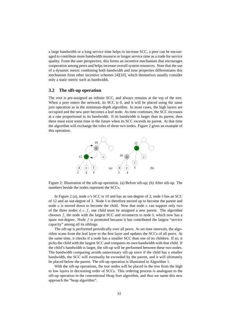
The root is pre-assigned an infinite SCC, and always remains at the top of the tree.When a peer enters the network, its SCC is 0, and it will be placed using the samejoin operation as in the minimum-depth algorithm. In most cases, the high layers areoccupied and the new peer becomes a leaf node. As time continues, the SCC increasesat a rate proportional to its bandwidth. If its bandwidth is larger than its parent, thenthere must exist some time in the future when its SCC exceeds its parent. At that timethe algorithm will exchange the roles of these two nodes. Figure 2 gives an example ofthis operation.
f e d
c b
a
f
e d
c a
b
10
10
12
5 4 3
12
5
4 3
(a) (b)
Figure 2: Illustration of the sift-up operation. (a) Before sift-up; (b) After sift-up. Thenumbers beside the nodes represent the SCCs.
In Figure 2 (a), nodea’s SCC is 10 and has an out-degree of 2; nodeb has an SCCof 12 and an out-degree of 3. Nodeb is therefore moved up to become the parent andnodea is moved down to become the child. Now that nodea can support only twoof the three nodesd, e, f , one child must be assigned a new parent. The algorithmchoosesf , the node with the largest SCC and reconnects to nodeb, which now has aspare out-degree. Nodef is promoted because it has contributed the largest “servicecapacity” among all its siblings.
The sift-up is performed periodically over all peers. At set time intervals, the algo-rithm scans from the leaf layer to the first layer and updates the SCCs of all peers. Atthe same time, it checks if a node has a smaller SCC than one of its children. If so, itpicks the child with the largest SCC and compares its own bandwidth with that child. Ifthe child’s bandwidth is larger, the sift-up will be performed between these two nodes.The bandwidth comparing avoids unnecessary sift-up since if the child has a smallerbandwidth, the SCC will eventually be exceeded by the parent, and it will ultimatelybe placed below the parent. The sift-up operation is illustrated in Algorithm 1.
With the sift-up operations, the tree nodes will be placed in the tree from the highto low layers in decreasing order of SCCs. This ordering process is analogous to thesift-up operation in the conventional Heap Sort algorithm, and thus we name this newapproach the “heap algorithm”.
35

Algorithm 1 Sift-up1: for i = N to i = 1 do2: for all P (j) in L(i) do3: Scc(j) ← B(i)×A(i) {update SCC}4: c ← the first child ofP (j)
{find the child with maximum SCC}5: for all P (k) that isP (j)’s child do6: if Scc(k) > Scc(c) then7: c ← k8: end if9: end for
{sift-up the child peerc}10: if Scc(c) > Scc(j) andB(c) > B(j) then11: for r = 1 to r = D(j) do12: s ← child of P (c) with minimumSCC13: P (s).parent ← P (j)14: removeP (s) from P (c)’s children list15: end for16: grandp ← P (j).parent17: P (grandp).child ← P (c)18: P (c).parent ← P (grandp)19: P (c).child ← P (j)20: P (j).parent ← P (c)21: end if22: end for23: end for
The algorithm moves peers up the tree in a gradual manner. This accounts for thefact that many peers may leave within a short time after their arrival [20][17], resultingin a large number of service interruptions if they are placed high in the tree upon arrival.In contrast, placing a new peer at the leaf layer first and then adjusting its positionaccording to its behavior can reduce this risk. The longer a peer stays in the network,the safer it is to be moved up the tree.
The sift-up procedure requires a per-node operation which involves an updating ofthe SCC, and potentially a peer exchange. The peer exchange requiresd time, whered is the average out-degree of the peers. So each pass of the sift-up operation requiresO(M) time.
3.3 Topology-aware delay optimization
A short overlay path does not necessarily means a short network delay due to the mis-matching between the logical overlay network and the physical underlying network [9].The heap algorithm addresses this problem in two ways. First, when a peer initiallyjoins the network, the algorithm provides a number of candidate parents, of which thenearest will be chosen. Second, for peers that are already in the network, the algo-rithm uses a parent switching technique to dynamically re-connect the peers so that theaverage network delay between the peers remains optimal.
Parent switching is performed between any two consecutive layers, (e.g.,Lk andLk+1). An example is given in Figure 3: due to changes in the underlying network,
36

L(k)
L(k+1)
optimization
agent
optimization set
L(k)
L(k+1)
(a) (b)
(c)
Figure 3: Topology-aware delay optimization.
the optimized mapping between the three pairs of peers in (a) is transformed to themapping in (b) to minimize the average delay. It can be seen that this combinatorialoptimization problem is NP-hard and when the number of peers in each layer is large(e.g. 2000), it can only be resolved using some approximate algorithms.
The heap algorithm assigns to each peer upon arrival anoptimization agent, whichis selected from the peers that have existed for a relatively long time and are thought tobe stable. During the streaming service, peers exchange neighbors information betweeneach other and periodically measure the network distances (in terms of delay) betweenthemselves and other peers, including their immediate neighbors, and the neighbors’neighbors, and so on. These data are reported to their optimization agent, which pe-riodically computes for a good solution for the peer mapping problem using a geneticalgorithm. The agent does not necessarily compute for all its associated peers, insteadit randomly selects a subset of peers, which form anoptimization group. A limitedpopulation size in the genetic algorithm allows a good solution to be obtained quickly,and thus is more suitable for a dynamic environment. When a solution is obtained, theagent coordinates the peers to adjust their connections. If an agent leaves, its associ-ated peers simply request from the server for a new agent. Figure 3 (c) illustrates theoptimization agent and grouping.
The approach of switching trees has also been studied in [8][2][9]. While thesestudies make use of fully distributed optimization schemes, the heap algorithm usesa hybrid approach: a subset of peers are optimized by a single agent, and there aremultiple such agents in the network. This mechanism has the advantage of beingsimple to implement. For example, Banerjee et al. define five deterministic localtransformations and one probabilistic transformation, which make the protocol muchmore complicated. The switch-tree in [8] also defines multiple transformations. Thesedistributed algorithms generally have a slower convergence speed than a centralizedscheme, which means they may require more reconnections between peers than theproposed hybrid approach.
3.4 Discussion
Accurate bandwidth estimates are critical for the heap algorithm and they should notentirely rely on the users’ settings. In the heap algorithm, the user-advertised band-
37

width is only taken as an upper bound; actual bandwidth estimates are derived from theactive end-to-end measurements as described in [5]. When a peer joins, its outboundbandwidth is set to zero, and an active measurement is launched between itself andanother peer in the leaf layer. The measured bandwidth is then used in the calculationof SCC. To keep the estimate up to date, the bandwidth is measured periodically forpeers whose bandwidths have not been fully utilized. The techniques of choosing theend host to transfer testing data, smoothing estimation and estimate discretization allfollow the methods introduced in [5].
A peer tree resulting from the sift-up operation integrates the characteristics of boththe bandwidth-ordered and time-ordered tree, since the peers are adjusted with a metricthat mixes bandwidth and time properties, and those peers at the higher layers eitherpossess high-bandwidths or long lifetimes, or both. As a hybrid of the two types ofbaseline tree, the new tree is expected to inherit their merits in both tree depth and treereliability.
4 Simulation methodology
An event-driven simulator has been developed to study the performance of the differentalgorithms. The following five algorithms are implemented:
• Minimum-depth algorithm: This algorithm follows that in [16][12][7], but with aminor modification – when a layer that can support a new peer is found, the newpeer chooses the nearest peer in terms of network delay (from up to 200 peers)in that layer as its parent. Since in practise a tree hierarchy may have thousandsof peers in a layer, imposing a limit to the number of candidates would be morepractical for implementation;
• Longest-first algorithm: This follows the scheme presented in [16].When a newpeer chooses its parent from the highest possible layer, it always chooses theoldest peer (from up to 200 peers) in that layer.
• Relaxed bandwidth-ordered algorithmandRelaxed time-ordered algorithm: Theseare two variants of the bandwidth-ordered and time-ordered algorithms as intro-duced in Section 3. The (strict) bandwidth-ordered and time-ordered trees arefound to have a extremely high protocol cost, which makes them unacceptable inpractise and only of theoretical value. Therefore, a modification is made to makethe compared scenarios more realistic – when a peer joins/rejoins the tree, it al-ways searches from the high to low layers to see if there is a smaller-bandwidthor younger peer, and if so, the identified peer is replaced with the new one. Theevicted peer, and possibly together with some of its children in the case of timeordering, are forced to rejoin the tree. This results in bandwidth/time orderinglocally within each layer and among parents and children, but not in a strict hier-archical structure; that is, a peer may have a smaller bandwidth/age than anothernon-child peer in the next layer. Since they still follow the basic ideas of band-width/time ordering, they are used for performance comparisons.
• Heap algorithm: This is implemented as introduced in Section 3, but with theparent switching disabled. It should be noted that such a technique can be appliedto any of the other algorithms previously documented. Disabling this componenthelps to reveal the performance of the proposed algorithm in its “naive” form,and also avoids any bias in comparison with other algorithms.
38

The GT-ITM transit-stub model [21] is used to generate an underlying networktopology consisting of 15600 nodes. Link delays between two transit nodes, transitnodes and stub nodes, and two stub nodes are chosen uniformly between[15, 25] ms,[5, 9] ms and[2, 4] ms, respectively. Of all the 15360 stub nodes, a fraction of themare randomly selected to participate in the peer tree. The server’s location is fixed at arandomly chosen stub node.
In all simulations, the root node’s bandwidth is set to 100; the peers’ outboundbandwidths follow a Bounded Pareto distribution1 with shape, lower bound and upperbound parameters set to 1.2, 0.5 and 100 respectively (denoted by BP(1.2, 0.5, 100)),with which 55.5% of the peers have out-degrees less than 1 and are therefore termed“free-riders”; the peers’ lifetimes follow a lognormal distribution with theµ (locationparameter) andσ (shape parameter) set to 6.0 and 2.0 respectively (denoted by LN(6.0,2.0)), which are chosen according to the findings in [20].
The simulation considers different network scales in terms of the average numberof peersM in a steady state. According toLittle’s Law, the peer arrival rateλ isdetermined fromM divided by the mean value of LN(6.0, 2.0). For the heap algorithm,the sift-up operation is performed every time 200 new peers join by default. Otherselections of parameters are also tested and the results are found to be consistent.
5 Performance evaluation
This section presents and discusses the performance results with respect to servicereliability, service delay, protocol overhead and the impact of sift-up frequency on treedepths.
5.1 Service reliability
Service reliability is measured by the average number of service interruptions experi-enced by a single peer during its lifetime in the steady state of a tree. The experimentsconsider the extreme case in which every peer departs abruptly without notification toothers, and hence results in a service interruption on each of its descendants. This met-ric reflects the stability of a tree in the most uncooperative and dynamic environment.
Figure 4 compares the performance of the five algorithms under different networksizes.
As expected, the minimum-depth algorithm performs the worst in most cases, be-cause it is designed completely blind of reliability. The longest-first algorithm hasvery limited improvement over the minimum-depth algorithm, as it operates in a veryconservative way when ordering the peers’ times.
It is surprising to see that the relaxed time-ordered algorithm performs worse thanthe heap algorithm. There are two reasons for this: first, the heap algorithm alsoachieves a partial time order in the process of sift-ups (the older peers are graduallymoved upward in the tree), and consequently benefits from this in terms of reliabil-ity; the second reason is that the heap algorithm builds a much shorter tree than therelaxed time-ordered algorithm, which means that a failed node generally introducesfewer service interruptions to its descendants.
1Previous studies [15][16][14] have shown that the bandwidths of peers exhibit characteristics of heavy-tailed distributions, a typical example of which is the Pareto distribution. Considering the practical limits ofpossible bandwidth values, a bounded Pareto distribution is used to model the peers’ bandwidths.
39
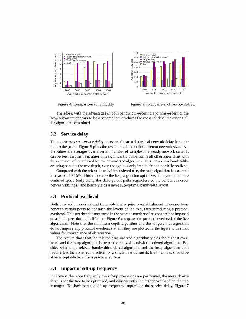
0
1
2
3
4
5
6
7
2000 5000 8000 11000 14000
Avg. number of peers in a steady state
Avg
. num
. of i
nte
rrup
tions
per
pee
r Minimum-depthRelaxed bandwidth-orderedLongest-firstRelaxed time-orderedHeap
Figure 4: Comparison of reliability.
0
100
200
300
400
500
600
700
2000 5000 8000 11000 14000
Avg. number of peers in a steady state
Avg
. ne
twor
k de
lay
(ms)
Minimum-depthRelaxed bandwidth-orderedLongest-firstRelaxed time-orderedHeap
Figure 5: Comparison of service delays.
Therefore, with the advantages of both bandwidth-ordering and time-ordering, theheap algorithm appears to be a scheme that produces the most reliable tree among allthe algorithms examined.
5.2 Service delay
The metricaverage service delaymeasures the actual physical network delay from theroot to the peers. Figure 5 plots the results obtained under different network sizes. Allthe values are averages over a certain number of samples in a steady network state. Itcan be seen that the heap algorithm significantly outperforms all other algorithms withthe exception of the relaxed bandwidth-ordered algorithm. This shows how bandwidth-ordering benefits the tree depth, even though it is only implicitly and partially realized.
Compared with the relaxed bandwidth-ordered tree, the heap algorithm has a smallincrease of 10-15%. This is because the heap algorithm optimizes the layout in a moreconfined space (only along the child-parent paths regardless of the bandwidth orderbetween siblings), and hence yields a more sub-optimal bandwidth layout.
5.3 Protocol overhead
Both bandwidth ordering and time ordering require re-establishment of connectionsbetween certain peers to optimize the layout of the tree, thus introducing a protocoloverhead. This overhead is measured in the average number of re-connections imposedon a single peer during its lifetime. Figure 6 compares the protocol overhead of the fivealgorithms. Note that the minimum-depth algorithm and the longest-first algorithmdo not impose any protocol overheads at all; they are plotted in the figure with smallvalues for convenience of observation.
The results show that the relaxed time-ordered algorithm yields the highest over-head, and the heap algorithm is better the relaxed bandwidth-ordered algorithm. Be-sides which, the relaxed bandwidth-ordered algorithm and the heap algorithm bothrequire less than one reconnection for a single peer during its lifetime. This should beat an acceptable level for a practical system.
5.4 Impact of sift-up frequency
Intuitively, the more frequently the sift-up operations are performed, the more chancethere is for the tree to be optimized, and consequently the higher overhead on the treemanager. To show how the sift-up frequency impacts on the service delay, Figure 7
40
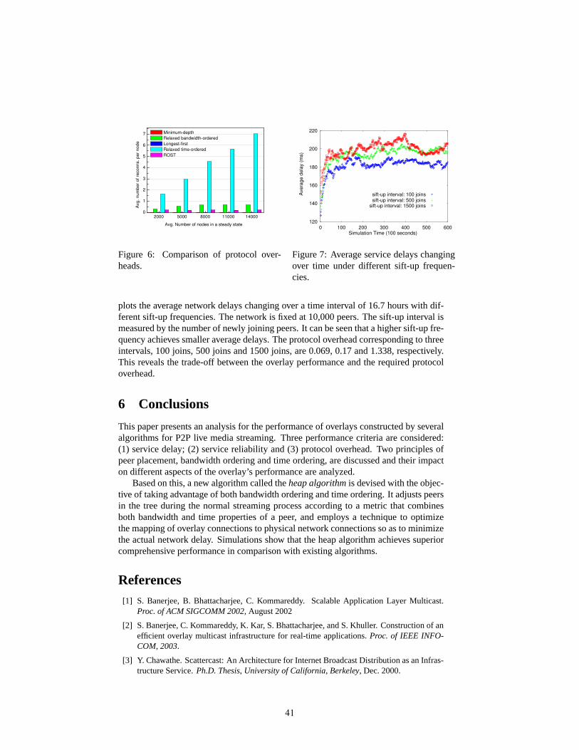
2000 5000 8000 11000 14000 0
1
2
3
4
5
6
7 A
vg
. n
um
be
r o
f re
co
nn
s.
pe
r n
od
e
Avg. Number of nodes in a steady state
Minimum-depth
Relaxed bandwidth-ordered
Longest-first
Relaxed time-ordered
ROST
Figure 6: Comparison of protocol over-heads.
120
140
160
180
200
220
0 100 200 300 400 500 600
Avera
ge d
ela
y (
ms)
Simulation Time (100 seconds)
sift-up interval: 100 joins sift-up interval: 500 joins
sift-up interval: 1500 joins
Figure 7: Average service delays changingover time under different sift-up frequen-cies.
plots the average network delays changing over a time interval of 16.7 hours with dif-ferent sift-up frequencies. The network is fixed at 10,000 peers. The sift-up interval ismeasured by the number of newly joining peers. It can be seen that a higher sift-up fre-quency achieves smaller average delays. The protocol overhead corresponding to threeintervals, 100 joins, 500 joins and 1500 joins, are 0.069, 0.17 and 1.338, respectively.This reveals the trade-off between the overlay performance and the required protocoloverhead.
6 Conclusions
This paper presents an analysis for the performance of overlays constructed by severalalgorithms for P2P live media streaming. Three performance criteria are considered:(1) service delay; (2) service reliability and (3) protocol overhead. Two principles ofpeer placement, bandwidth ordering and time ordering, are discussed and their impacton different aspects of the overlay’s performance are analyzed.
Based on this, a new algorithm called theheap algorithmis devised with the objec-tive of taking advantage of both bandwidth ordering and time ordering. It adjusts peersin the tree during the normal streaming process according to a metric that combinesboth bandwidth and time properties of a peer, and employs a technique to optimizethe mapping of overlay connections to physical network connections so as to minimizethe actual network delay. Simulations show that the heap algorithm achieves superiorcomprehensive performance in comparison with existing algorithms.
References[1] S. Banerjee, B. Bhattacharjee, C. Kommareddy. Scalable Application Layer Multicast.
Proc. of ACM SIGCOMM 2002, August 2002
[2] S. Banerjee, C. Kommareddy, K. Kar, S. Bhattacharjee, and S. Khuller. Construction of anefficient overlay multicast infrastructure for real-time applications.Proc. of IEEE INFO-COM, 2003.
[3] Y. Chawathe. Scattercast: An Architecture for Internet Broadcast Distribution as an Infras-tructure Service.Ph.D. Thesis, University of California, Berkeley, Dec. 2000.
41

[4] Y. Chu, A. Ganjam, T. S. E. Ng, S. G. Rao, K. Sripanidkulchai, J. Zhan and H. Zhang.Early Experience with an Internet Broadcast System Based on Overlay Multicast.Proc. ofUSENIX 2004 Annual Technical Conference.
[5] Y. Chu, S. G. Rao, S. Seshan, and H. Zhang. Enabling conferencing applications on theInternet using an overlay multicast architecture.Proc. of ACM SIGCOMM 2001.
[6] Y. Chu, S. Rao, and H. Zhang. A Case for End System Multicast.Proc. of ACM SIGMET-RICS, June 2000.
[7] M. Guo, M. Ammar. Scalable live video streaming to cooperative clients using time shiftingand video patching.Proc. of IEEE INFOCOM 2004.
[8] D. Helder and S. Jamin. End-host Multicast Communication Using Switch-tree Protocols.In Proc. of Internation Conference on Global and Peer-to-Peer Computing on Large ScaleDistributed Systems, 2002.
[9] Y. Liu, Z. Zhuang, Li Xiao. A Distributed Approach to Solving Overlay MismatchingProblem. InProc. of 24th International Conference on Distributed Computing Systems(ICDCS’04)
[10] Wei Tsang Ooi. Dagster: contributor-aware end-host multicast for media streaming inheterogeneous environment.Proc. of Multimedia Computing and Networking (MMCN),2005.
[11] Venkata N. Padmanabhan, Helen J. Wang, Philip A. Chou. Resilient Peer-to-Peer Stream-ing. 11th IEEE International Conference on Network Protocols (ICNP), 2003.
[12] V. N. Padmanabhan, H. J. Wang, P. A. Chou, and K. Sripanidkulchai. Distributing Stream-ing Media Content Using Cooperative Networking.ACM NOSSDAV, May 2002.
[13] D. Pendarakis, S. Shi, D. Verma, and M. Waldvogel. ALMI: An Application Level Multi-cast Infrastructure. In Proc. of3rd Usenix Symposium on Internet Technologies and Systems(USITS), March 2001.
[14] S. Saroiu, P. Gummadi and S. Gribble A Measurement Study of Peer-to-Peer File SharingSystems.Proc. of Multimedia Computing and Networking (MMCN), 2002.
[15] S. Sen and J. Wang. Analyzing peer-to-peer traffic across large networks.IEEE/ACMTrans. on Networking.Vol. 12, No. 2, April 2004.
[16] K. Sripanidkulchai, A. Ganjam, B. Maggs and H. Zhang. The feasibility of supportinglarge-scale live streaming applications with dynamic application end-points.Proc. of ACMSIGCOMM, 2004, Portland, Oregon, USA.
[17] K. Sripanidkulchai, B. Maggs and H. Zhang An analysis of live streaming workloads onthe Internet.Proc. of the 4th ACM SIGCOMM IMC, Oct., 2004. Italy.
[18] G. Tan, S. A. Jarvis, D. P. Spooner and G. R. Nudd. On Efficient and Robust OverlayConstruction for Large-scale P2P Live Media Streaming.TR-2005-02, Dept. of ComputerScience, University of Warwick, UK.
[19] D. A. Tran, K. A. Hua, and T. T. Do. A peer-to-peer architecture for media streaming.IEEEJournal on Selected Areas in Communications (JSAC), Special Issue on Recent Advancesin Service Overlay Networks. 22, Jan. 2004.
[20] E. Veloso, V. Almeida, W. Meira, A. Bestavros, and S. Jin. A Hierarchical Characterizationof A Live Streaming Media Workload.IEEE/ACM Trans. on Networking, 12(5), 2004.
[21] E. W. Zegura, K. Calvert and S. Bhattacharjee. How to Model an Internetwork.Proc. ofIEEE INFOCOM ’96, San Francisco, CA.
42

A Practical Guide to Measuring the
Hurst Parameter
Richard G. Clegg
June 28, 2005
Abstract
This paper describes, in detail, techniques for measuring the Hurst parameter.Measurements are given on artificial data both in a raw form and corrupted invarious ways to check the robustness of the tools in question. Measurements arealso given on real data, both new data sets and well-studied data sets. All dataand tools used are freely available for download along with simple “recipes”which any researcher can follow to replicate these measurements.
1 Introduction and Background
Long-Range Dependence (LRD) is a statistical phenomenon which has receivedmuch attention in the field of telecommunications in the last ten years. A time-series is described as possessing LRD if it has correlations which persist overall time scales. A good guide to LRD is given by [3] and a summary in thecontext of telecommunications is given by [4, chapter one] (from which some ofthe material in this paper is taken). In the early nineties, LRD was measured intime-series derived from internet traffic [8]. The importance of this is that LRDcan impact heavily on queuing. LRD is characterised by the parameter H, theHurst parameter, (named for a hydrologist who pioneered the field in the fifties[7]) where H ∈ (1/2, 1) indicates the presence of LRD. There are a numberof different statistics which can be used to estimate the Hurst parameter andseveral papers have been written comparing these estimators both in theory andpractice [16, 15, 1]. The aim of this paper is not to make a rigorous comparisonof the estimators but, instead, to present a simple and readable guide to whata researcher can expect from attempting to assess whether LRD is absent orpresent in a data set. All the tools used are available online using free software.Software can be downloaded from:http://www.richardclegg.org/lrdsources/software/
1.1 A Brief Introduction to Long-Range Dependence
Let {Xt : t ∈ N} be a time-series which is weakly stationary (that is it has afinite mean and the covariance depends only on the separation or “lag” betweentwo points in the series). Let ρ(k) be the auto-correlation function (ACF) ofXt.
43

Definition 1. The ACF, ρ(k) for a weakly-stationary time series, {Xt : t ∈ N}is given by
ρ(k) =E [(Xt − µ)(Xt+k − µ)]
σ2,
where E [Xt] is the expectation of Xt, µ is the mean and σ2 is the variance.
There are a number of different definitions of LRD in use in the literature.A commonly used definition is given below.
Definition 2. The time-series Xt is said to be long-range dependent if∑
∞
k=−∞ρ(k)
diverges.
Often the specific functional form
ρ(k) ∼ Cρk−α, (1)
is assumed where Cρ > 0 and α ∈ (0, 1). Note that the symbol ∼ is used hereand throughout this paper to mean asymptotically equal to or f(x) ∼ g(x) ⇒f(x)/g(x) = 1 as x → ∞ or, where indicated, as x → 0. The parameter α isrelated to the Hurst parameter via the equation α = 2− 2H.
If (1) holds then a similar definition can be shown to hold in the frequencydomain.
Definition 3. The spectral density f(λ) of a function with ACF ρ(k) and vari-ance σ2 can be defined as
f(λ) =σ2
2π
∞∑
k=−∞
ρ(k)eikλ,
where λ is the frequency, σ2 is the variance and i =√−1.
Note that this definition of spectral density comes from the Wiener-Kninchinetheorem [17].
Definition 4. The weakly-stationary time-series Xt is said to be long-range
dependent if its spectral density obeys
f(λ) ∼ Cf |λ|−β ,
as λ→ 0, for some Cf > 0 and some real β ∈ (0, 1).
The parameter β is related to the Hurst parameter by H = (1 + β)/2.LRD relates to a number of other areas of statistics, notably the presence of
statistical self-similarity. Self-similarity can be characterised by a self-similarityparameter H and the increment process of a self-similar process with stationaryincrements and H ∈ (1/2, 1) is itself an LRD process with Hurst parameterH. Indeed analysis of telecommunications traffic is often described in terms ofself-similarity and not long-range dependence.
In summary, LRD can be thought of in two ways. In the time domain it man-ifests as a high degree of correlation between distantly separated data points. Inthe frequency domain it manifests as a significant level of power at frequenciesnear zero. LRD is, in many ways, a difficult statistical property to work with.In the time-domain it is measured only at high lags (strictly at infinite lags) of
44

the ACF — those very lags where only a few samples are available and wherethe measurement errors are largest. In the frequency domain it is measured atfrequencies near zero, again where it is hardest to make measurements. Timeseries with LRD converge slowly to their mean. While the Hurst parameter isperfectly well-defined mathematically, it will be shown that it is, in fact, a verydifficult property to measure in real life.
1.2 Long-Range Dependence in Telecommunications
In their classic paper, Leland et al [8] measure traffic past a point on an EthernetLocal Area Network. They conclude that “In the case of Ethernet LAN traffic,self-similarity is manifested in the absence of a natural length of a ‘burst’; atevery time scale ranging from a few milliseconds to minutes and hours, burstsconsist of bursty sub-periods separated by less burst sub-periods. We also showthat the degree of self-similarity (defined via the Hurst parameter) typicallydepends on the utilisation level of the Ethernet and can be used to measure‘burstiness’ of LAN traffic.” Since then, a number of authors have replicatedthese experiments on a variety of measurments of internet traffic and the ma-jority found evidence of LRD or related multi-fractal behaviour. Summaries aregiven in [14, 18]. The reason for the interest in the area is that LRD can, insome circumstances, negatively impact network performance. The exact detailsof the scale and nature of the effect are uncertain and depend on the particularLRD process being considered.
2 Measuring the Hurst Parameter
While the Hurst parameter is perfectly well-defined mathematically, measuringit is problematic. The data must be measured at high lags/low frequencies wherefewer readings are available. Early estimators were biased and converged onlyslowly as the amount of data available increased. All estimators are vulnerableto trends in the data, periodicity in the data and other sources of corruption.Many estimators assume specific functional forms for the underlying model andperform poorly if this is misspecified. The techniques in this paper are chosen fora variety of reasons. The R/S parameter, aggregated variance and periodogramare well-known techniques which have been used for some time in measurementsof the Hurst parameter. The local Whittle and wavelet techniques are newertechniques which generally fare well in comparative studies. All the techniqueschosen have freely available code which can be used with free software to esti-mate the Hurst parameter.
The problems with real-life data are worse than those faced when measuringartificial data. Real life data is likely to have periodicity (due to, for example,daily usage patterns), trends and perhaps quantisation effects if readings aretaken to a given precision. The naive researcher taking a data set and runningit through an off-the-shelf method for estimating the Hurst parameter is likelyto end up with a misleading answer or possibly several different misleadinganswers.
45

2.1 Data sets to be studied
A large number of methods are used for generating data exhibiting LRD. Areview of some of the better known methods are given in [2]. In this paper trialdata sets with LRD and a known Hurst parameter are generated using fractionalauto-regressive integrated moving average (FARIMA) modelling and fractionalGaussian noise (FGN).
A FARIMA model is a well-known time series modelling technique. It is amodification of the standard time series ARIMA (p, d, q) model. An ARIMAmodel is defined by
(1−p∑
j=1
φjBj)(1−B)dXi = (1−
q∑
j=1
θjBj)εi,
where p is the order of the AR part of the model, the φi are the AR parameters,p is the order of the MA part of the model, the θj are the MA parameters, d ∈ Z
is the order of differencing, the εi are i.i.d. noise (usually normally distributedwith zero mean) and B is the backshift operator defined by B(Xt) = Xt−1. If,instead of being an integer, the model is changed so that d ∈ (0, 1/2) then themodel is a FARIMA model. If the φi and θi are chosen so that the model isstationary and d ∈ (0, 1/2) then the model will be LRD with H = d + 1/2.FARIMA processes were proposed by [6] and a description in the context ofLRD can be found in [3, pages 59–66].
Fractional Brownian Motion is a process BH(t) for t ≥ 0 obeying,
• BH(0) = 0 almost surely,
• BH(t) is a continuous function of t,
• The distribution of B(t) obeys
P [BH(t + k)−BH(t) ≤ x] = (2π)−1
2 k−H
x∫
−∞
exp
( −u2
2k2H
)
du,
where H ∈ (1/2, 1) is the Hurst parameter. The process BH(t) is known asfractional Brownian motion (FBM) and its increments are known as fractionalGaussian noise (FGN). FBM is a self-similar process with self-similarity parame-ter H and FGN exhibits long-range dependence with Hurst parameter H. WhenH = 1/2 in the above, then the process is the well known Weiner process (Brow-nian motion) and the increments are independent (Gaussian noise). A numberof authors have described computationally efficient methods for generating FGNand FBM. The one used in this paper is due to [11].
Data generated from these models will be tested using the various measure-ment techniques and then the same data set will be corrupted in several waysto see how this disrupts measurements:
• Addition of zero mean AR(1) model with a high degree of short-rangecorrelation (Xt = 0.9Xt−1 + εt). This simulates a process with high de-gree of short-range correlation which might be mistaken for a long-rangecorrelation.
46

• Addition of periodic function (sine wave) — ten complete cycles of a sinwave are added to the signal. This simulates a seasonal effect in the data,for example, a daily usage pattern.
• Addition of linear trend. This simulates growth in the data, for examplethe data might be a sample of network traffic at a time of day when thenetwork is growing busier as time continues.
The noise signals are normalised so the standard deviation of the corruptingsignal is identical to the standard deviation of the original LRD signal to whichit is being added. Note that, strictly speaking, while the addition of an AR(1)model does not change the LRD in the model, techincally the addition of atrend or of periodic noise makes the time-series non-stationary and hence thetime-series produces are, strictly speaking, not really LRD.
In addition, some real-life traffic traces are studied to provide insight intohow well different measurements agree across data sets with and without varioustransforms being applied to clean the data. The data sets used are listed below.
• The famous (and much-studied) Bellcore data [9] which was collected in1989 and has been used for a large number of studies since. Note that,unfortunately, the exact traces used in [8] are not available for download.This data is available online at:http://ita.ee.lbl.gov/html/contrib/BC.html
• A data set collected at the University of York in 2001 which consists ofa tcpdump trace of 67 minutes of incoming and outgoing data from theexternal link to the university from the rest of the internet.
Various techniques are tried to filter real-life traces in addition to makingmeasurements purely on the raw data. These methods have been selected fromthe literature as commonly used by researchers in the field. Often in such cases,a high pass filter would be used to remove periodicity and trends, however,since LRD measurements are most important at low-frequency that is an obvi-ously inappropriate technique. The techniques used to pre-process data beforeestimating H are listed below.
• Transform to log of original data (only appropriate if data is positive).
• Removal of mean and linear trend (that is, subtract the best fit line Y =at + b for constant a and b).
• Removal of high order best-fit polynomial of degree ten (the degree tenwas chosen after higher degrees showed evidence of overfitting).
2.2 Measurement techniques
The measurement techniques used in this paper can only be described brieflybut references to fuller descriptions with mathematical details are given. Thetechniques used here are chosen for various reasons. The R/S statistic, aggre-gated variance and periodogram are well-known techniques with a considerablehistory of use in estimating long-range dependence. The wavelet analysis tech-nique and local Whittle estimator are newer techniques which perform well incomparative studies and have strong theoretical backing.
47
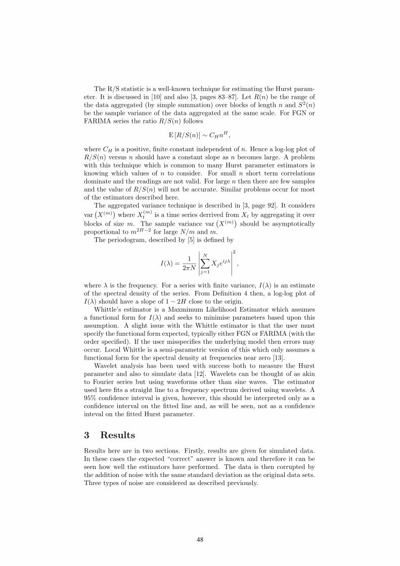
The R/S statistic is a well-known technique for estimating the Hurst param-eter. It is discussed in [10] and also [3, pages 83–87]. Let R(n) be the range ofthe data aggregated (by simple summation) over blocks of length n and S2(n)be the sample variance of the data aggregated at the same scale. For FGN orFARIMA series the ratio R/S(n) follows
E [R/S(n)] ∼ CHnH ,
where CH is a positive, finite constant independent of n. Hence a log-log plot ofR/S(n) versus n should have a constant slope as n becomes large. A problemwith this technique which is common to many Hurst parameter estimators isknowing which values of n to consider. For small n short term correlationsdominate and the readings are not valid. For large n then there are few samplesand the value of R/S(n) will not be accurate. Similar problems occur for mostof the estimators described here.
The aggregated variance technique is described in [3, page 92]. It considers
var(
X(m))
where X(m)t is a time series derrived from Xt by aggregating it over
blocks of size m. The sample variance var(
X(m))
should be asymptoticallyproportional to m2H−2 for large N/m and m.
The periodogram, described by [5] is defined by
I(λ) =1
2πN
∣
∣
∣
∣
∣
∣
N∑
j=1
Xjeijλ
∣
∣
∣
∣
∣
∣
2
,
where λ is the frequency. For a series with finite variance, I(λ) is an estimateof the spectral density of the series. From Definition 4 then, a log-log plot ofI(λ) should have a slope of 1− 2H close to the origin.
Whittle’s estimator is a Maxmimum Likelihood Estimator which assumesa functional form for I(λ) and seeks to minimise parameters based upon thisassumption. A slight issue with the Whittle estimator is that the user mustspecify the functional form expected, typically either FGN or FARIMA (with theorder specified). If the user misspecifies the underlying model then errors mayoccur. Local Whittle is a semi-parametric version of this which only assumes afunctional form for the spectral density at frequencies near zero [13].
Wavelet analysis has been used with success both to measure the Hurstparameter and also to simulate data [12]. Wavelets can be thought of as akinto Fourier series but using waveforms other than sine waves. The estimatorused here fits a straight line to a frequency spectrum derived using wavelets. A95% confidence interval is given, however, this should be interpreted only as aconfidence interval on the fitted line and, as will be seen, not as a confidenceinteval on the fitted Hurst parameter.
3 Results
Results here are in two sections. Firstly, results are given for simulated data.In these cases the expected “correct” answer is known and therefore it can beseen how well the estimators have performed. The data is then corrupted bythe addition of noise with the same standard deviation as the original data sets.Three types of noise are considered as described previously.
48

In the second section results are given for real data. The York data isanalysed as a time series of bytes per unit time for two different time units.The Bellcore data is analysed both in terms of interarrival times and in termsof bytes per unit time. Note that, strictly speaking, the interarrival times donot consititute a proper “time-series” since the time units between readings arenot constant.
3.1 Results on Simulated Data
For each of the simulation methods chosen, traces have been generated. Eachtrace is 100,000 points of data. Hurst parameters of 0.7 and 0.9 have beenchosen to represent a low and a high level of long-range dependence in data.The errors on the wavelet estimator are a 95% confidence interval on the fittedregression line (not, as might be thought, the Hurst parameter measured).
Table 1 shows results for various FGN models. Three runs each are donewith a Hurst parameter of 0.7 and then 0.9. Firstly it should be noted that, inall case, for H=0.7 all estimators are relatively close when no noise is applied.The R/S method performs worst, as it consistently underestimates the Hurstparameter. The addition of AR(1) noise confuses all the methods with the LocalWhittle performing particularly poorly. The correct answer is well outside theconfidence intervals of the Wavelet estimate after this addition. Addition of asine wave or a trend causes trouble for the aggregated variance method but thefrequency domain methods (wavelets and local Whittle) do not seem greatlyaffected.
When considering runs with Hurst parameter H=0.9, the R/S method getsa considerable underestimate even with no corrupting noise. Note also that theR/S and aggregated variance method actually produce quite different estimatesfor the three runs. Most methods seem to perform badly with the AR(1) noisecorruption. Again the frequency domain methods seem to be able to cope withthe sine wave and with the addition of a trend.
Table 2 shows a variety of results for FARIMA models. The first threeruns are for a FARIMA (0, d, 0) model (that is one with no AR or MA compo-nents) and with a Hurst parameter H = 0.7. In this case, all methods peformadequately with no noise (although the R/S plot perhaps underestimates theanswer). Addition of AR(1) noise causes problems for the R/S plot, wavelet andlocal Whittle methods and to a lesser extent the periodogram. The addition ofa sin wave and a trend causes problems for the aggregated variance.
For a FARIMA (1, d, 1) model with H = 0.7 and with the AR parameterφ1 = 0.5 and the MA parameter θ1 = 0.5 (implying a moderate degree of shortrange correlation) all estimators provide a reasonable result for the uncorruptedseries. As before, the wavelet and local Whittle method seem relatively robustto the addition of a trend. The AR(1) noise again causes problems for most ofthe methods.
For a FARIMA (0, d, 0) model with H = 0.9 the R/S method under predictsthe Hurst parameter but all others perform well in the absence of noise. TheAR(1) noise causes problems for the local Whittle and wavelet methods and thesine wave and trend cause problems for the aggregated variance.
For a FARIMA (1, d, 1) model with H = 0.9 and with the AR parameterφ1 = 0.5 and the MA parameter θ1 = 0.5 (implying, as before, a moderatedegree of short range correlation) all estimators do relatively well initially. The
49

Added R/S Plot Aggreg. Period. Wavelet LocalNoise Variance ogram Estimate Whittle
100,000 points FGN — H= 0.7 — run one.None 0.66 0.668 0.686 0.707 ± 0.013 0.72AR(1) 0.767 0.657 0.794 0.888 ± 0.034 0.904Sin 0.667 0.969 0.692 0.707 ± 0.013 0.787Trend 0.66 0.968 0.777 0.707 ± 0.013 0.766
100,000 points FGN — H= 0.7 — run two.None 0.641 0.692 0.7 0.694 ± 0.007 0.721AR(1) 0.775 0.671 0.795 0.882 ± 0.036 0.902Sin 0.66 0.97 0.705 0.694 ± 0.007 0.788Trend 0.641 0.968 0.769 0.694 ± 0.007 0.765
100,000 points FGN — H= 0.7 — run three.None 0.636 0.69 0.704 0.708 ± 0.009 0.723AR(1) 0.734 0.654 0.79 0.876 ± 0.038 0.905Sin 0.64 0.969 0.709 0.708 ± 0.009 0.787Trend 0.636 0.971 0.783 0.708 ± 0.009 0.77
100,000 points FGN — H= 0.9 — run one.None 0.782 0.864 0.905 0.901 ± 0.009 0.934AR(1) 0.805 0.784 0.88 0.969 ± 0.042 1.066Sin 0.772 0.961 0.907 0.901 ± 0.009 0.945Trend 0.782 0.958 0.928 0.901 ± 0.009 0.939
100,000 points FGN — H= 0.9 — run two.None 0.862 0.837 0.891 0.902 ± 0.003 0.933AR(1) 0.856 0.76 0.877 0.969 ± 0.038 1.062Sin 0.858 0.955 0.894 0.902 ± 0.003 0.943Trend 0.862 0.954 0.921 0.902 ± 0.003 0.938
100,000 points FGN — H= 0.9 — run two.None 0.793 0.884 0.907 0.904 ± 0.007 0.93AR(1) 0.818 0.802 0.871 0.972 ± 0.041 1.066Sin 0.8 0.967 0.91 0.904 ± 0.007 0.943Trend 0.794 0.959 0.924 0.904 ± 0.007 0.936
Table 1: Results for Fractional Gaussian Noise models plus various forms ofnoise.
50
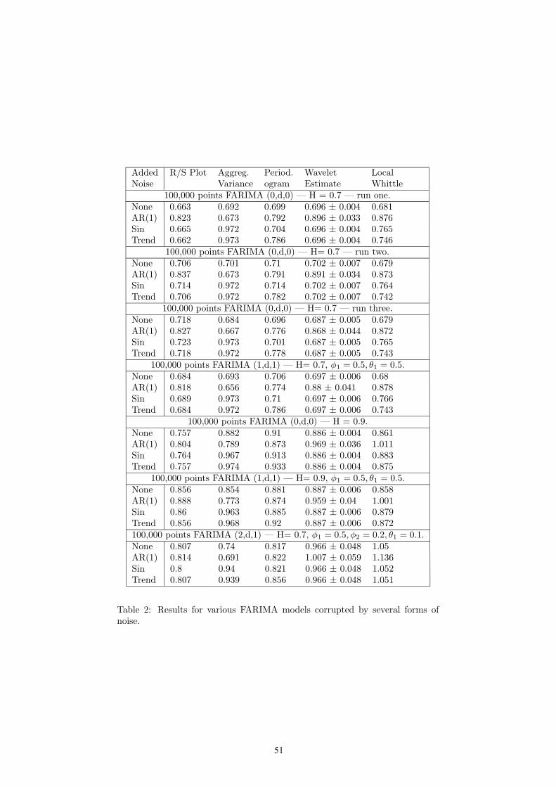
Added R/S Plot Aggreg. Period. Wavelet LocalNoise Variance ogram Estimate Whittle
100,000 points FARIMA (0,d,0) — H = 0.7 — run one.None 0.663 0.692 0.699 0.696 ± 0.004 0.681AR(1) 0.823 0.673 0.792 0.896 ± 0.033 0.876Sin 0.665 0.972 0.704 0.696 ± 0.004 0.765Trend 0.662 0.973 0.786 0.696 ± 0.004 0.746
100,000 points FARIMA (0,d,0) — H= 0.7 — run two.None 0.706 0.701 0.71 0.702 ± 0.007 0.679AR(1) 0.837 0.673 0.791 0.891 ± 0.034 0.873Sin 0.714 0.972 0.714 0.702 ± 0.007 0.764Trend 0.706 0.972 0.782 0.702 ± 0.007 0.742
100,000 points FARIMA (0,d,0) — H= 0.7 — run three.None 0.718 0.684 0.696 0.687 ± 0.005 0.679AR(1) 0.827 0.667 0.776 0.868 ± 0.044 0.872Sin 0.723 0.973 0.701 0.687 ± 0.005 0.765Trend 0.718 0.972 0.778 0.687 ± 0.005 0.743
100,000 points FARIMA (1,d,1) — H= 0.7, φ1 = 0.5, θ1 = 0.5.None 0.684 0.693 0.706 0.697 ± 0.006 0.68AR(1) 0.818 0.656 0.774 0.88 ± 0.041 0.878Sin 0.689 0.973 0.71 0.697 ± 0.006 0.766Trend 0.684 0.972 0.786 0.697 ± 0.006 0.743
100,000 points FARIMA (0,d,0) — H = 0.9.None 0.757 0.882 0.91 0.886 ± 0.004 0.861AR(1) 0.804 0.789 0.873 0.969 ± 0.036 1.011Sin 0.764 0.967 0.913 0.886 ± 0.004 0.883Trend 0.757 0.974 0.933 0.886 ± 0.004 0.875
100,000 points FARIMA (1,d,1) — H= 0.9, φ1 = 0.5, θ1 = 0.5.None 0.856 0.854 0.881 0.887 ± 0.006 0.858AR(1) 0.888 0.773 0.874 0.959 ± 0.04 1.001Sin 0.86 0.963 0.885 0.887 ± 0.006 0.879Trend 0.856 0.968 0.92 0.887 ± 0.006 0.872100,000 points FARIMA (2,d,1) — H= 0.7, φ1 = 0.5, φ2 = 0.2, θ1 = 0.1.None 0.807 0.74 0.817 0.966 ± 0.048 1.05AR(1) 0.814 0.691 0.822 1.007 ± 0.059 1.136Sin 0.8 0.94 0.821 0.966 ± 0.048 1.052Trend 0.807 0.939 0.856 0.966 ± 0.048 1.051
Table 2: Results for various FARIMA models corrupted by several forms ofnoise.
51

Filter R/S Plot Aggreg. Period. Wavelet LocalType Variance ogram Estimate Whittle
York trace (bytes/second) — 4047 pointsNone 0.749 0.88 1.186 0.912 ± 0.052 0.981Log 0.758 0.894 1.105 0.921 ± 0.039 0.932Trend 0.749 0.873 1.212 0.912 ± 0.052 0.981Poly 0.756 0.723 0.732 0.895 ± 0.04 0.972
York trace (bytes/tenth) — 40467 pointsNone 0.826 0.924 0.928 0.909 ± 0.012 0.881Trend 0.826 0.923 0.932 0.909 ± 0.012 0.881Poly 0.827 0.892 0.863 0.909 ± 0.012 0.878
Table 3: Analysis of bytes/unit time data collected at the University of York.
corruption produces the same problems with the same estimators — that is tosay, wavelets and local Whittle do not cope with the AR(1) noise and Aggregatedvariance reacts badly to the sine wave and local trend.
For a FARIMA (2, d, 1) model with H = 0.9 and with the AR parametersφ1 = 0.5, φ2 = 0.2 and the MA parameter θ1 = 0.1 indicating quite strongshort-range correlations, none of the estimators perform particularly well. Theaggregated variance estimate is initially close and remains so in the presenceof AR(1) noise but presented with these results, a researcher would certainlynot know the Hurst parameter of the underlying model from looking at theresults given by the estimators. All five are producing different results in mostcases (there is some aggreement between the R/S plot and periodogram but itwould be hard to put this down to anything more than coincidence and, in anycase, they are agreeing on an incorrect value for the Hurst parameter). It isinteresting that, even in this relatively simple case where the theoretical correctresult is known, five well-known estimators of the Hurst parameter all fail toget the correct answer.
3.2 Results on Real Data
In analysing the real data it is hard to know where to begin. Since the genuineanswer (if, indeed, it can be really said that there is a genuine answer) is notknown it cannot be said that one result is more “right” than another. Thesuggested methods for preprocessing data (taking logs, removing a linear trendand removing a best fit polynomial — in this case of order ten) have all beenfound in the literature on measuring the Hurst parameter.
Table 3 shows analysis of data collected at the University of York. The samedata set is analysed firstly as a series of bytes/second and then as bytes/tenthof a second. While theoretically the results should be the same, in practice thisis not the case. Obviously there are only one tenth as many points in the dataset when seconds are used rather than tenths of seconds. Firstly, looking at thedata aggregated over a time period of one second, there is no good agreementbetween estimators. The periodogram estimate is hopelessly out of the correctrange. The other estimators, while in the range (1/2, 1) show no particularagreement. Of the suggested filtering techniques, little changes between them
52

Filter R/S Plot Aggreg. Period. Wavelet LocalType Variance ogram Estimate WhittleBellcore data BC-Aug89 (interarrival times) — first 360,000 points.
None 0.73 0.742 0.762 0.73 ± 0.018 0.661Log 0.722 0.806 0.797 0.77 ± 0.02 0.652Trend 0.73 0.74 0.762 0.73 ± 0.018 0.661Poly 0.73 0.733 0.751 0.73 ± 0.018 0.66Bellcore data BC-Aug89 (interarrival times) — second 360,000 points.None 0.709 0.703 0.742 0.746 ± 0.025 0.655Log 0.721 0.795 0.779 0.778 ± 0.011 0.673Trend 0.709 0.703 0.742 0.746 ± 0.025 0.655Poly 0.709 0.691 0.732 0.746 ± 0.025 0.654
Bellcore data BC-Aug89 (bytes/10ms) — first 1000 secs.None 0.707 0.8 0.817 0.786 ± 0.017 0.822Trend 0.707 0.797 0.815 0.786 ± 0.017 0.822Poly 0.707 0.789 0.787 0.786 ± 0.017 0.822
Bellcore data BC-Aug89 (bytes/10ms) — second 1000 secs.None 0.62 0.802 0.808 0.762 ± 0.012 0.825Trend 0.62 0.802 0.808 0.762 ± 0.012 0.825Poly 0.618 0.786 0.777 0.762 ± 0.012 0.824
Table 4: Analysis of bytes/unit time and interarrival times for the Bellcore datawith various methods to attempt to remove non-stationary components.
except that removal of a polynomial greatly reduces the estimate found by theperiodogram and slightly reduces the estimate found by aggregated variance.No conclusion can realistically be drawn about the data from these results.
Considering the data aggregated into tenths of a second time units the pic-ture is somewhat clearer. Taking a log of data was impossible at this time scaledue to presence of zeros. The estimators, with the exception of the R/S plot areall relatively near H = 0.9. While it seems somewhat arbitrary to ignore theresults of the R/S plot it should be remembered that this technique performedpoorly with high Hurst parameter measurements on theoretical data and un-derestimated badly in those cases. No great difference is observed from anyof the suggested filtering techniques except, perhaps, a slight reduction in theaggregated variance and periodogram results from removal of a polynomial. Atentative conclusion from this data would be that 0.85 < H < 0.95 and that theR/S plot is inaccurate for this trace.
In the case of the Bellcore measurements, the data has been split into twosections and analysed seperately for interarrival times and for bytes per unittime. Considering first the interarrival times, all estimators seem to have aresult which is not too distant from H = 0.7 in both cases. The various filteringtechniques tried do little to change this. It is hard to come to a really robustconclusion since the estimators are as high as 0.806 (aggregated variance aftertaking logs) and as low as 0.652 (local Whittle after taking logs).
When the bytes per unit time are considered, the log technique cannot beused due to zeros in the data. The most comfortable conclusion abou this datamight be that the Hurst parameter is somewhere around H = 0.8 with the R/S
53

plot underestimating again. As before, it is hard to reach a strong conclusion onthe exact Hurst parameter. Certainly it would be foolish to take the confidenceintervals on the wavelet estimator at face value. The various filters tried seem tomake little difference except perhaps a slight reduction in the answer given bysome estimators after the polynomial is removed. A tentative conclusion mightbe that 0.75 < H < 0.85 for this data with the R/S plot being in error.
4 Conclusion
This paper has looked at measuring the Hurst parameter, firstly in the case ofartificial data contaminated by various types of noise and secondly in the case ofreal data with various filters to try to improve the performance of the estimatorsused.
The most striking conclusion of this paper is that measuring the Hurst pa-rameter, even in artificial data, is very hit and miss. In the artificial data withno corrupting noise, some estimators performed very poorly indeed. Confidenceintervals given should certainly not be taken at face value (indeed should beconsidered as next to worthless).
Corrupting noise can affect the measurements badly and different estimatorsare affected in by different types of noise. In particular, frequency domainestimators (as might be expected) are robust to the addition of sinusoidal noiseor a trend. All estimators had problems in some circumstances with the additionof a heavy degree of short-range dependence even though this, in theory, doesnot change the long-range dependence of the time series.
When considering real data, researchers are advised to use extreme cau-tion. A researcher relying on the results of any single estimator for the Hurstparameter is likely to be drawing false conclusions, no matter how sound thetheoretical backing for the estimator in question. While simple filtering tech-niques are suggested in the literature for improving the performance of Hurstparameter estimation, they had little or no effect on the data analysed in thispaper.
All the data and tools used in this paper are available for download fromthe web and can be found at:http://www.richardclegg.org/lrdsources/software/
References
[1] J.-M. Bardet, G. Lang, G. Oppenheim, A. Phillipe, S. Stoev, and M. S.Taqqu. Semi-parametric estimation of the long-range dependence param-eter: A survey. In P. Doukhan, G. Oppenheim, and M. S. Taqqu, edi-tors, Theory and Applications of Long-Range Dependence, pages 557–577.Birkhauser, 2003.
[2] J.-M. Bardet, G. Lang, G. Oppenheim, A. Phillipe, and M. S. Taqqu.Generators of long-range dependent processes: A survey. In P. Doukhan,G. Oppenheim, and M. S. Taqqu, editors, Theory and Applications of Long-
Range Dependence, pages 579–623. Birkhauser, 2003.
[3] J. Beran. Statistics For Long-Memory Processes. Chapman and Hall, 1994.
54

[4] R. G. Clegg. Statistics of Dynamic Networks. PhD thesis, Dept. of Math.,Uni. of York., York., 2004. Available online at:www.richardclegg.org/pubs/thesis.pdf.
[5] J. Geweke and S. Porter-Hudak. The estimation and application of longmemory time series models. J. Time Ser. Anal., 4:221–238, 1983.
[6] C. W. J. Granger and R. Joyeux. An introduction to long-range time seriesmodels and fractional differencing. J. Time Ser. Anal., 1:15 – 30, 1980.
[7] H. E. Hurst. Long-term storage capacity of reservoirs. Transactions of the
American Society of Civil Engineers, pages 770–808, 1951.
[8] W. E. Leland, M. S. Taqqu, W. Willinger, and D. V. Wilson. On theself-similar nature of Ethernet traffic. In D. P. Sidhu, editor, Proc. ACM
SIGCOMM, pages 183–193, San Francisco, California, 1993.
[9] W. E. Leland and D. V. Wilson. High time-resolution measurement andanalysis of lan traffic: Implications for lan interconnection. Proc. IEEE
INFOCOM, pages 1360–1366, April 1991.
[10] B. B. Mandelbrot and J. R. Wallis. Computer experiments with fractionalgaussian noises. Water Resources Research, 5:228–267, 1969.
[11] V. Paxson. Fast, approximate synthesis of fractional gaussian noise forgenerating self-similar network traffic. Computer Comm. Rev., 27:5–18,1997.
[12] R. H. Riedi. Multifractal processes. In P. Doukhan, G. Oppenheim, andM. S. Taqqu, editors, Theory And Applications Of Long-Range Dependence,pages 625–716. Birkhauser, 2003.
[13] P. M. Robinson. Gaussian semiparametric estimation of long-range depen-dence. The Annals of Statistics, 23:1630–1661, 1995.
[14] Z. Sahinoglu and S. Tekinay. On multimedia networks: Self similar trafficand network performance. IEEE Communications Magazine, pages 48–52,January 1999.
[15] M. S. Taqqu and V. Teverovsky. Robustness of Whittle type estimatorsfor time series with long-range dependence. Stochastic Models, 13:723–757,1997.
[16] M.S. Taqqu, V. Teverovsky, and W. Willinger. Estimators for long-rangedependence: an empirical study. Fractals, 3(4):785–788, 1995.
[17] N. Weiner. Generalized harmonic analysis. Acta. Math., 55:178–258, 1930.
[18] W. Willinger, V. Paxson, R. H. Riedi, and M. S. Taqqu. Long-range de-pendence and data network traffic. In P. Doukhan, G. Oppenheim, andM. S. Taqqu, editors, Theory And Applications Of Long-Range Dependence,pages 373–407. Birkhauser, 2003.
55

56
An Alternative Algorithm to Multiply a Vectorby a Kronecker Represented Descriptor
Paulo Fernandes∗ Ricardo Presotto† Afonso Sales‡
Thais Webber§
Abstract
The key operation to obtain stationary and transient solutions of models de-scribed by Kronecker structured formalisms using iterative methods is the Vector-Descriptor product. This operation is usually performed with the Shuffle algo-rithm, which was proposed to Stochastic Automata Networks, but it is also cur-rently used by Stochastic Petri Nets and Performance Evaluation Process Alge-bra solvers. This paper presents an alternative algorithm to perform the Vector-Descriptor product, called Slice algorithm. The numerical advantages of this newalgorithm over the previous one is shown to SAN models, in which the compu-tational costs are compared. Finally, we discuss some possible optimizations ofthe Slice algorithm and implementation issues regarding parallel versions of bothalgorithms.
1 Introduction
All formalisms used to model complex systems are based on a structured descrip-tion. This is particularly the case of Markovian performance and reliability evaluationmodels. A myriad of formalisms is available in the research community, e.g., Stochas-tic Activity Networks [13], Queueing Networks [9], Stochastic Petri Nets (SPN) [1],Performance Evaluation Process Algebra (PEPA) [11], and Stochastic Automata Net-works (SAN) [12]. Among such formalisms we are specially interested in those whichuse Tensor (or Kronecker) Algebra to represent the infinitesimal generator of the un-derlying Markov chain [7, 8]. Such tensor formula representation is referred in theliterature as descriptor.
The key operation to perform iterative solutions, both stationary and transient, ofmodels described as a descriptor is the multiplication by a probability vector [14]. Suchoperation is performed using the Shuffle algorithm [8] which has a quite efficient way tohandle tensor structures and takes advantage of several techniques developed to SAN[4], to PEPA [10], and to SPN [6].
The main purpose of this paper is to propose an alternative algorithm to performthe vector-descriptor product, which we call Slice. The main advantage of the Slicealgorithm is the possible reduction of computational cost (number of multiplications)
∗PUCRS, [email protected] (corresponding author). P. Fernandes is partially funded by CNPq/Brazil.†PUCRS, [email protected]‡PUCRS, [email protected]§PUCRS, [email protected], T. Webber is funded by CAPES/Brazil.
57

for very sparse tensor components. Such reduction is achieved keeping the compacttensor format of the descriptor. In some way, the Slice algorithm can be consideredas a trade-off between the sparse matrix approach used for straightforward Markovchains, and the fully tensor approach used by the Shuffle algorithm.
Nevertheless, this paper does not exploit the Slice algorithm possibilities to its lim-its, since very few considerations are made concerning possible optimizations. In par-ticular, we do not analyse the possible benefits of automata reordering according tofunctional dependencies, which was deeply studied for the Shuffle algorithm. Also apossible hybrid approach using Shuffle and Slice algorithms are not discussed in de-tail. Actually, we focus our contribution in the presentation of an original way to handlethe vector-descriptor product and we present encouraging measures to develop furtherstudies based on this new approach.
This paper is organized with a brief introduction to the descriptor structure (Section2). Section 3 presents the basic operation of the vector-descriptor product followedby sections describing the Shuffle algorithm principle (Section 3.1) and the proposedSlice algorithm (Section 3.2). In Section 4, we show some comparative measures ofboth Shuffle and Slice algorithms applied to two distinct structured models. Finally theconclusion points out some future works necessary to raise the Slice algorithm to asimilar level of optimization as the level already obtained by the Shuffle algorithm.
2 Tensor Represented Descriptor
Regardless of the structured formalism adopted, e.g., SAN, SPN, PEPA, the basicprinciple consists in the representation of a whole system by a collection of subsystemswith an independent behavior (local behavior) and occasional interdependencies (syn-chronized behavior). According to the formalism, the primitives to describe local andsynchronized behaviors may change their denomination, the reader interested in theformalisms definitions can found information in [12, 4] for SAN, in [1, 6] for SPN,and [11, 10] for PEPA.
For the purpose of this paper it is only important to consider that, unlike the non-structured approaches, e.g., straightforward Markov chains, a structured model is notdescribed by a single sparse matrix, but instead, by a descriptor. For a structured modelwith N subsystems and E synchronizing primitives, the descriptor (Q) is an algebraicformula containing N + 2NE matrices:
Q =
N⊕
gi=1
Q(i)l +
E∑
j=1
N⊗
gi=1
Q(i)
e+
j
+
N⊗
gi=1
Q(i)
e−
j
(1)
where:
• Q(i)l represents N matrices describing each local behaviors of the ith subsystem;
• Q(i)
e+
j
represents NE matrices describing the occurrence of synchronizing primi-
tive e in the ith subsystem;
• and Q(i)
e−
j
represents NE analogous matrices describing the diagonal adjustment
of synchronizing primitive e in the ith subsystem.
58

Table 1 details descriptor Q, which is composed of two separated parts: a tensorsum corresponding to the local events; a sum of tensor products corresponding to thesynchronizing events [8]. The tensor sum operation of the local part can be decomposedinto the ordinary sum of N normal factors, i.e., a sum of tensor products where allmatrices but one are identity matrices1. Therefore, in this first part, only the non-identity matrices (Q(i)
l ) need to be stored.
∑
Q(1)l ⊗
gIn2
⊗g· · · ⊗
gInN−1
⊗g
InN
In1⊗g
Q(2)l ⊗
g· · · ⊗
gInN−1
⊗g
InN
N...
In1⊗g
In2⊗g· · · ⊗
gQ
(N−1)l ⊗
gInN
In1⊗g
In2⊗g· · · ⊗
gInN−1
⊗g
Q(N)l
2E
Q(1)
e+
1
⊗g
Q(2)
e+
1
⊗g· · · ⊗
gQ
(N−1)
e+
1
⊗g
Q(N)
e+
1
e+ ...
Q(1)
e+
E
⊗g
Q(2)
e+
E
⊗g· · · ⊗
gQ
(N−1)
e+
E
⊗g
Q(N)
e+
E
Q(1)
e−
1
⊗g
Q(2)
e−
1
⊗g· · · ⊗
gQ
(N−1)
e−
1
⊗g
Q(N)
e−
1
e− ...
Q(1)
e−
E
⊗g
Q(2)
e−
E
⊗g· · · ⊗
gQ
(N−1)
e−
E
⊗g
Q(N)
e−
E
Table 1: SAN descriptor
3 Vector-Descriptor Product
The vector-descriptor product operation corresponds to the product of a vector v,as big as the product state space (
∏N
i=1 ni), by descriptor Q. Since the descriptor is theordinary sum of N + 2E tensor products, the basic operation of the vector-descriptorproduct is the multiplication of vector v by a tensor product of N matrices:
N+2E∑
j=1
v ×
N⊗
gi=1
Q(i)j
(2)
where Q(i)j corresponds to Ini
, Q(i)l , Q
(i)e+ , or Q
(i)e− according to the tensor product term
where it appears.For simplicity in this section, we describe the Shuffle and Slice algorithms for the
basic operation vector × tensor product term omitting index j from equation 2, i.e.:
v ×
N⊗
gi=1
Q(i)
(3)
1Iniis an identity matrix of order ni.
59
3.1 Shuffle Algorithm
The Shuffle algorithm is described in this section without any considerations aboutoptimizations for the evaluation of functional elements. A thorough study about ma-trices reordering and generalized tensor algebra properties with this objective can befound in [8]. All those optimizations aim to reduce the overhead of evaluate func-tional elements, but they do not change the number of multiplications needed by theShuffle algorithm. Therefore, we ignore the functional elements in the context of thispaper, and the basic operation (equation 3) is simplified to consider classical (⊗) andnot generalized (⊗
g) tensor products.
The basic principle of the Shuffle algorithm concerns the application of the decom-position of a tensor product in the ordinary product of normal factors property:
Q(1) ⊗ . . .⊗Q(N) = (Q(1) ⊗ In2⊗ . . .⊗ InN−1
⊗ InN) ×
(In1⊗Q(2) ⊗ . . .⊗ InN−1
⊗ InN) ×
...(In1⊗ In2
⊗ . . .⊗Q(N−1) ⊗ InN) ×
(In1⊗ In2
⊗ . . .⊗ InN−1⊗Q(N))
(4)
Rewritten the basic operation (equation 3) according to this property:
v ×[
N∏
i=1
Inlefti⊗Q(i) ⊗ Inrighti
]
(5)
where nlefti corresponds to the product of the order of all matrices before the ith
matrix of the tensor product term, i.e.,∏i−1
k=1 nk (particular case: nleft1 = 1) andnrighti corresponds to the product of the order of all matrices after the ith matrix ofthe tensor product term, i.e.,
∏Nk=i+1 nk (particular case: nrightN = 1).
Hence, the Shuffle algorithm consists in multiplying successively a vector by eachnormal factor. More precisely, vector v is multiplied by the first normal factor, then theresulting vector is multiplied by the next normal factor and so on until the last factor.In fact, the multiplication of a vector v by the ith normal factor corresponds to shufflethe elements of v in order to assemble nlefti×nrighti vectors of size ni and multiplythem by matrix Q(i). Therefore, assuming that matrix Q(i) is stored as a sparse matrix,the number of multiplications needed to multiply a vector by the ith normal factor is:
nlefti × nrighti × nzi (6)
where nzi corresponds to the number of nonzero elements of the ith matrix of thetensor product term (Q(i)). Considering the number of multiplications to all normalfactors of a tensor product term, we obtain [8]:
N∏
i=1
ni ×N
∑
i=1
nzi
ni
(7)
3.2 Slice Algorithm
Slice is an alternative algorithm to perform the vector-descriptor product not basedonly on the decomposition of a tensor product in the ordinary product of normal factors
60
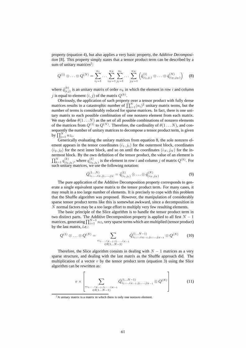
property (equation 4), but also applies a very basic property, the Additive Decomposi-tion [8]. This property simply states that a tensor product term can be described by asum of unitary matrices2:
Q(1) ⊗ . . .⊗Q(N) =
n1∑
i1=1
. . .
nN∑
iN=1
n1∑
j1=1
. . .
nN∑
jN=1
(
q(1)(i1,j1) ⊗ . . .⊗ q
(N)(iN ,jN )
)
(8)
where q(k)(i,j) is an unitary matrix of order nk in which the element in row i and column
j is equal to element (i, j) of the matrix Q(k).Obviously, the application of such property over a tensor product with fully dense
matrices results in a catastrophic number of∏N
i=1(ni)2 unitary matrix terms, but the
number of terms is considerably reduced for sparse matrices. In fact, there is one uni-tary matrix to each possible combination of one nonzero element from each matrix.We may define θ(1 . . .N) as the set of all possible combinations of nonzero elementsof the matrices from Q(1) to Q(N). Therefore, the cardinality of θ(1 . . . N), and con-sequently the number of unitary matrices to decompose a tensor product term, is givenby
∏N
i=1 nzi.Generically evaluating the unitary matrices from equation 8, the sole nonzero el-
ement appears in the tensor coordinates (i1, j1) for the outermost block, coordinates(i2, j2) for the next inner block, and so on until the coordinates (iN , jN ) for the in-nermost block. By the own definition of the tensor product, the value of an element is∏N
k=1 q(k)(ik ,jk), where q
(k)(ik,jk) is the element in row i and column j of matrix Q(k). For
such unitary matrices, we use the following notation:
Q(1...N)i1,...,iN ,j1,...,jN
= q(1)(i1,j1) ⊗ . . .⊗ q
(N)(iN ,jN ) (9)
The pure application of the Additive Decomposition property corresponds to gen-erate a single equivalent sparse matrix to the tensor product term. For many cases, itmay result in a too large number of elements. It is precisely to cope with this problemthat the Shuffle algorithm was proposed. However, the manipulation of considerablysparse tensor product terms like this is somewhat awkward, since a decomposition inN normal factors may be a too large effort to multiply very few resulting elements.
The basic principle of the Slice algorithm is to handle the tensor product term intwo distinct parts. The Additive Decomposition property is applied to all first N − 1matrices, generating
∏N−1i=1 nzi very sparse terms which are multiplied (tensor product)
by the last matrix, i.e.:
Q(1) ⊗ . . .⊗Q(N) =∑
∀i1,...,iN−1,j1,...,jN−1
∈θ(1...N−1)
Q(1...N−1)i1,...,iN−1,j1,...,jN−1
⊗Q(N) (10)
Therefore, the Slice algorithm consists in dealing with N − 1 matrices as a verysparse structure, and dealing with the last matrix as the Shuffle approach did. Themultiplication of a vector v by the tensor product term (equation 3) using the Slicealgorithm can be rewritten as:
v ×
∑
∀i1,...,iN−1,j1,...,jN−1
∈θ(1...N−1)
Q(1...N−1)i1,...,iN−1,j1,...,jN−1
⊗Q(N)
(11)
2A unitary matrix is a matrix in which there is only one nonzero element.
61

Applying the distributive property, equation 11 can be rewritten as:
∑
∀i1,...,iN−1,j1,...,jN−1
∈θ(1...N−1)
v ×(
Q(1...N−1)i1,...,iN−1,j1,...,jN−1
⊗Q(N))
(12)
We call each term of the previous equation as Additive Unitary Normal Factor,since it is composed of an unitary matrix times a standard normal factor. The decom-position in normal factors applied to each additive unitary normal factor of equation 12results in:
v ×[(
Q(1...N−1)i1,...,iN−1,j1,...,jN−1
⊗ InN
)
×(
InleftN⊗Q(N)
)]
(13)
It is important to notice that the first multiplication takes only nN elements of vectorv and it corresponds to the product of this sliced vector (called vs) by the single scalarwhich is the nonzero element of matrix Q
(1...N−1)i1,...,iN−1,j1,...,jN−1
. The resulting vector,
called v′
s, must then be multiplied only once by matrix Q(N), since all other positionsof the intermediate vector (except those in v′
s) are zero.The application of the Slice algorithm must generate the nonzero element (c) of
matrix Q(1...N−1)i1,...,iN−1,j1,...,jN−1
. Hence, it must pick a slice of vector v (called vs) accord-ing to the row position of element c, and multiply all elements of vs by c. In fact, thismultiplication by a scalar corresponds to the first multiplication by a normal factor ofequation 13. The resulting vector, called v′
s, must be multiplied by the matrix Q(N)
(second multiplication in equation 13), accumulating the result (rs) in the positions ofthe resulting vector r corresponding to the column position of element c.
The Slice algorithm (Algorithm 1) can be summarize for all Additive Unitary Nor-mal Factors in the operation:
r = v ×[(
Q(1...N−1)i1,...,iN−1,j1,...,jN−1
⊗ InN
)
×(
InleftN⊗Q(N)
)]
Algorithm 1 Slice Algorithm
1: for all i1, . . . , iN−1, j1, . . . , jN−1 ∈ θ(1 . . .N − 1) do2: c←
∏N−1k=1 q
(k)(ik ,jk)
3: slice vs from v according to i1, . . . , iN−1
4: v′s ← c× vs
5: rs ← v′s ×Q(N)
6: add rs to r according to j1, . . . , jN−1
7: end for
The computational cost (number of needed multiplications) of the slice algorithmconsiders: the number of unitary matrices (
∏N−1i=1 nzi); the cost to generate the nonzero
element of each unitary matrix (N−2); the cost to multiply it by each element of slicedvector vs (nN ); and the cost to multiply vs by the last matrix Q(N) (nzN ), i.e.:
N−1∏
i=1
nzi ×[
(N − 2) + nN + nzN
]
(14)
62
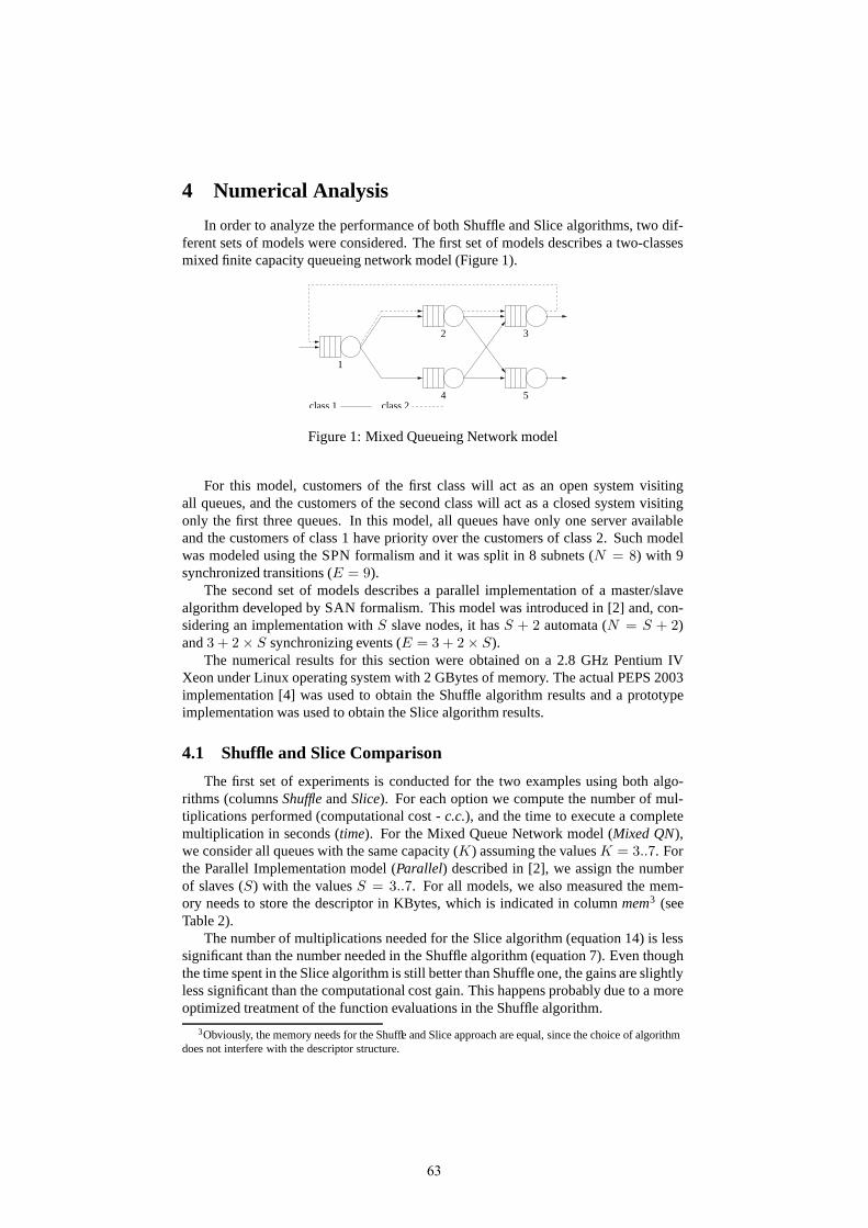
4 Numerical Analysis
In order to analyze the performance of both Shuffle and Slice algorithms, two dif-ferent sets of models were considered. The first set of models describes a two-classesmixed finite capacity queueing network model (Figure 1).
1
2
4 5
3
class 1 class 2
Figure 1: Mixed Queueing Network model
For this model, customers of the first class will act as an open system visitingall queues, and the customers of the second class will act as a closed system visitingonly the first three queues. In this model, all queues have only one server availableand the customers of class 1 have priority over the customers of class 2. Such modelwas modeled using the SPN formalism and it was split in 8 subnets (N = 8) with 9synchronized transitions (E = 9).
The second set of models describes a parallel implementation of a master/slavealgorithm developed by SAN formalism. This model was introduced in [2] and, con-sidering an implementation with S slave nodes, it has S + 2 automata (N = S + 2)and 3 + 2× S synchronizing events (E = 3 + 2× S).
The numerical results for this section were obtained on a 2.8 GHz Pentium IVXeon under Linux operating system with 2 GBytes of memory. The actual PEPS 2003implementation [4] was used to obtain the Shuffle algorithm results and a prototypeimplementation was used to obtain the Slice algorithm results.
4.1 Shuffle and Slice Comparison
The first set of experiments is conducted for the two examples using both algo-rithms (columns Shuffle and Slice). For each option we compute the number of mul-tiplications performed (computational cost - c.c.), and the time to execute a completemultiplication in seconds (time). For the Mixed Queue Network model (Mixed QN),we consider all queues with the same capacity (K) assuming the values K = 3..7. Forthe Parallel Implementation model (Parallel) described in [2], we assign the numberof slaves (S) with the values S = 3..7. For all models, we also measured the mem-ory needs to store the descriptor in KBytes, which is indicated in column mem3 (seeTable 2).
The number of multiplications needed for the Slice algorithm (equation 14) is lesssignificant than the number needed in the Shuffle algorithm (equation 7). Even thoughthe time spent in the Slice algorithm is still better than Shuffle one, the gains are slightlyless significant than the computational cost gain. This happens probably due to a moreoptimized treatment of the function evaluations in the Shuffle algorithm.
3Obviously, the memory needs for the Shuffle and Slice approach are equal, since the choice of algorithmdoes not interfere with the descriptor structure.
63
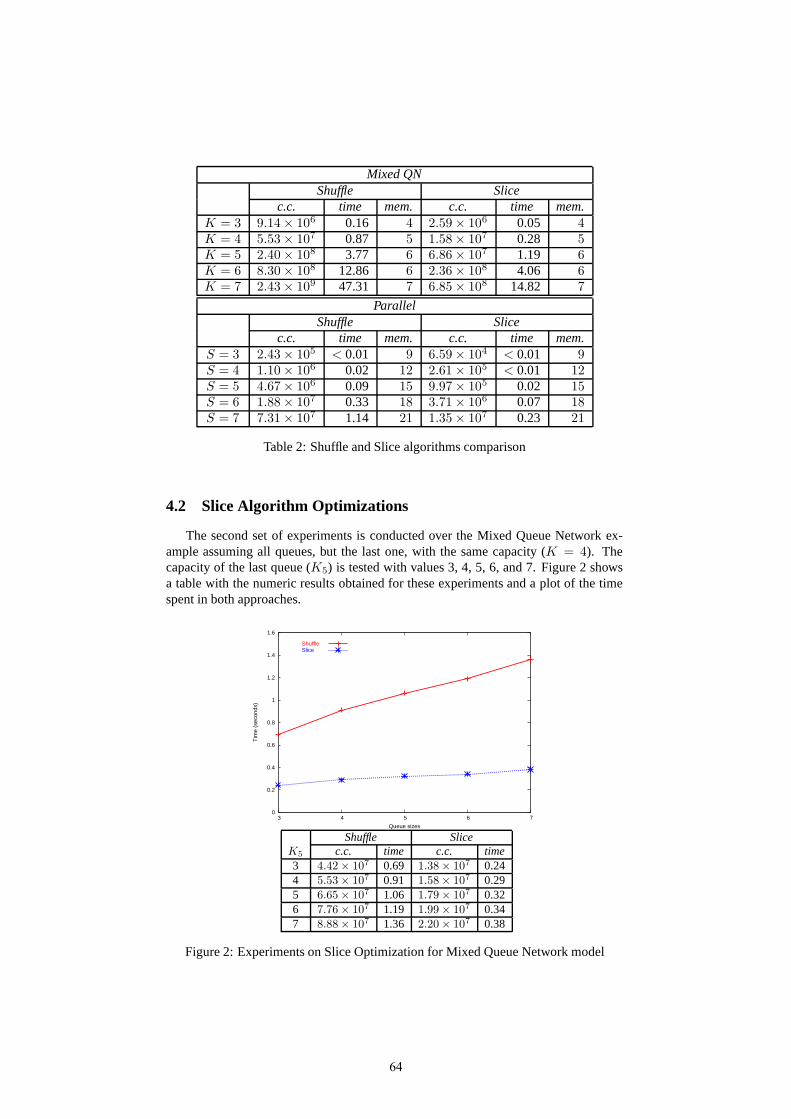
Mixed QNShuffle Slice
c.c. time mem. c.c. time mem.K = 3 9.14× 10⁶ 0.16 4 2.59× 10⁶ 0.05 4K = 4 5.53× 10⁷ 0.87 5 1.58× 10⁷ 0.28 5K = 5 2.40× 10⁸ 3.77 6 6.86× 10⁷ 1.19 6K = 6 8.30× 10⁸ 12.86 6 2.36× 10⁸ 4.06 6K = 7 2.43× 10⁹ 47.31 7 6.85× 10⁸ 14.82 7
ParallelShuffle Slice
c.c. time mem. c.c. time mem.S = 3 2.43× 10⁵ < 0.01 9 6.59× 10⁴ < 0.01 9S = 4 1.10× 10⁶ 0.02 12 2.61× 10⁵ < 0.01 12S = 5 4.67× 10⁶ 0.09 15 9.97× 10⁵ 0.02 15S = 6 1.88× 10⁷ 0.33 18 3.71× 10⁶ 0.07 18S = 7 7.31× 10⁷ 1.14 21 1.35× 10⁷ 0.23 21
Table 2: Shuffle and Slice algorithms comparison
4.2 Slice Algorithm Optimizations
The second set of experiments is conducted over the Mixed Queue Network ex-ample assuming all queues, but the last one, with the same capacity (K = 4). Thecapacity of the last queue (K5) is tested with values 3, 4, 5, 6, and 7. Figure 2 showsa table with the numeric results obtained for these experiments and a plot of the timespent in both approaches.
0
0.2
0.4
0.6
0.8
1
1.2
1.4
1.6
3 4 5 6 7
Tim
e (s
econ
ds)
Queue sizes
ShuffleSlice
Shuffle SliceK5 c.c. time c.c. time3 4.42× 10⁷ 0.69 1.38× 10⁷ 0.244 5.53× 10⁷ 0.91 1.58× 10⁷ 0.295 6.65× 10⁷ 1.06 1.79× 10⁷ 0.326 7.76× 10⁷ 1.19 1.99× 10⁷ 0.347 8.88× 10⁷ 1.36 2.20× 10⁷ 0.38
Figure 2: Experiments on Slice Optimization for Mixed Queue Network model
64

Observing equations 7 and 14, it is possible to notice that, unlike the cost of theShuffle algorithm, the cost of the Slice algorithm is less dependent on the order of thelast matrix. This can be verified by the results in Figure 2, since both Slice and Shufflecurves have clearly different behaviors.
0
0.05
0.1
0.15
0.2
0.25
3 4 5 6 7
Tim
e (s
econ
ds)
Number of slaves
OriginalReordered
Non Ordered ReorderedS c.c. time c.c. time3 6.59× 10⁴ < 0.01 3.67× 10⁴ < 0.014 2.61× 10⁵ < 0.01 1.37× 10⁵ < 0.015 9.97× 10⁵ 0.02 4.92× 10⁵ 0.016 3.71× 10⁶ 0.07 1.73× 10⁶ 0.037 1.35× 10⁷ 0.23 5.95× 10⁶ 0.09
Figure 3: Experiments on Slice Optimization for Parallel Implementation model
The last set of experiments (Figure 3) shows the effect of automata reordering forthe Parallel Implementation model. This model has one very large automaton (40states) and all other automata with only 3 states. For these experiments, only the resultsof the Slice algorithm are indicated. The left hand side columns (Non Ordered) indicatethe results obtained for the example with the larger automaton appearing at the begin-ning. The right hand side columns (Reordered) indicate the results obtained puttingthe largest automaton as the last one. The results show clearly the improvements inthe number of multiplications as well as in the time spent. Such encouraging resultsuggests that many other optimizations could still be found to the Slice algorithm.
It is important to notice that an analysis of the functional evaluations for the Slicealgorithm may reveal further optimizations, but as said in the introduction such analysisis out of the scope of this paper.
5 Conclusion
This paper proposes a different way to perform vector-descriptor product. The newSlice algorithm has shown a better overall performance than the traditional Shufflealgorithm for all examples tested. In fact, the Shuffle algorithm would only be moreefficient for quite particular cases in which the descriptor matrices would be nearly full.Even though we could imagine such tensor products (with only nearly full matrices),we were not able to generate a real model with such characteristics. It seems that realcase models have naturally sparse matrices. The local part of a descriptor is naturallyvery sparse due to the tensor sum structure. The synchronizing primitives are mostly
65
used to describe exceptional behaviors, therefore it lets the synchronizing part of thedescriptor also quite sparse.
As a matter of fact, the Slice algorithm seems to offer a good trade-off between theunique sparse matrix approach used for straightforward Markov chains and the puretensor approach of the Shuffle algorithm. It is much more memory efficient than theunique sparse matrix approach, and it would only be slower than the Shuffle algorithmin hypothetical models with nearly full matrices. However, even for those hypotheticalmodels, the Slice approach may be used for some terms of the descriptor. Such hy-brid approach could analyze which algorithm should be used to each one of the tensorproduct terms of the descriptor.
Besides the immediate future works to develop further experiments with the Slicealgorithm already mentioned in the previous section, we may also foresee studies con-cerning parallel implementations. The prototyped parallel implementation of the Shuf-fle algorithm [3] has already shown consistent gains to solve particularly slow SANmodels. Nevertheless, the Shuffle algorithm parallelization suffers an important limi-tation that consists in the passing of a whole tensor product term to each parallel node.This is a problem since all nodes must compute multiplications of the whole vector vby a tensor product term that usually has nonzero elements in many positions.
The Slice algorithm can offer a more effective parallelization since its AdditiveUnitary Normal Factors only affect few positions of vector v. A parallel node couldreceive only similar terms and, therefore, not handle the whole vector v. This can bespecially interesting for parallel machines with nodes with few memory resources.
Concentrating back in the sequential implementation, our first results with the Slicealgorithm prototype were very encouraging, but we expect to have many improvementsto do before integrate this new algorithm in a new version of the PEPS software tool[4]. As we said before, this paper is just a first step for this new approach and muchnumerical studies have to be done. However, the current version of the Slice algorithmalready shows better results than Shuffle.
References
[1] M. Ajmone-Marsan, G. Conte, and G. Balbo. A Class of Generalized Stochas-tic Petri Nets for the Performance Evaluation of Multiprocessor Systems. ACMTransactions on Computer Systems, 2(2):93–122, 1984.
[2] L. Baldo, L. Brenner, L. G. Fernandes, P. Fernandes, and A. Sales. PerformanceModels for Master/Slave Parallel Programs. Electronic Notes In Theoretical Com-puter Science, 128(4):101–121, April 2005.
[3] L. Baldo, L. G. Fernandes, P. Roisenberg, P. Velho, and T. Webber. Parallel PEPSTool Performance Analysis using Stochastic Automata Networks. In M. Done-lutto, D. Laforenza, and M. Vanneschi, editors, Euro-Par 2004 International Con-ference on Parallel Processing, volume 3149 of Lecture Notes in Computer Sci-ence, pages 214–219, Pisa, Italy, August/September 2004. Springer-Verlag Hei-delberg.
[4] A. Benoit, L. Brenner, P. Fernandes, B. Plateau, and W. J. Stewart. The PEPSSoftware Tool. In Computer Performance Evaluation / TOOLS 2003, volume2794 of LNCS, pages 98–115, Urbana, IL, USA, 2003. Springer-Verlag Heidel-berg.
66

[5] L. Brenner, P. Fernandes, and A. Sales. The Need for and the Advantages of Gen-eralized Tensor Algebra for Kronecker Structured Representations. InternationalJournal of Simulation: Systems, Science & Technology, 6(3-4):52–60, February2005.
[6] G. Ciardo, R. L. Jones, A. S. Miner, and R. Siminiceanu. SMART: StochasticModel Analyzer for Reliability and Timing. In Tools of Aachen 2001 Interna-tional Multiconference on Measurement, Modelling and Evaluation of Computer-Communication Systems, pages 29–34, Aachen, Germany, September 2001.
[7] M. Davio. Kronecker Products and Shuffle Algebra. IEEE Transactions on Com-puters, C-30(2):116–125, 1981.
[8] P. Fernandes, B. Plateau, and W. J. Stewart. Efficient descriptor - Vector multi-plication in Stochastic Automata Networks. Journal of the ACM, 45(3):381–414,1998.
[9] E. Gelenbe. G-Networks: Multiple Classes of Positive Customers, Signals, andProduct Form Results. In Performance, volume 2459 of Lecture Notes in Com-puter Science, pages 1–16. Springer-Verlag Heidelberg, 2002.
[10] S. Gilmore and J. Hillston. The PEPA Workbench: A Tool to Support a ProcessAlgebra-based Approach to Performance Modelling. In Computer PerformanceEvaluation, pages 353–368, 1994.
[11] S. Gilmore, J. Hillston, L. Kloul, and M. Ribaudo. PEPA nets: a structured per-formance modelling formalism. Performance Evaluation, 54(2):79–104, 2003.
[12] B. Plateau and K. Atif. Stochastic Automata Networks for modelling parallelsystems. IEEE Transactions on Software Engineering, 17(10):1093–1108, 1991.
[13] W. H. Sanders and J. F. Meyer. Stochastic Activity Networks: Formal Definitionsand Concepts. In Lectures on Formal Methods and Performance Analysis : FirstEEF/Euro Summer School on Trends in Computer Science, volume 2090 of Lec-ture Notes in Computer Science, pages 315–343, Berg En Dal, The Netherlands,July 2001. Springer-Verlag Heidelberg.
[14] W. J. Stewart. Introduction to the numerical solution of Markov chains. PrincetonUniversity Press, 1994.
67

68
A moment-based estimation method for
extreme probabilities
Arpad Tari∗, Miklos Telek† and Peter Buchholz‡
Abstract
The performance analysis of highly reliable and fault tolerant systemsrequires the investigation of events with extremely low or high proba-bilities. This paper presents a simplified numerical method to bound theextreme probabilities based on the moments of the distribution. This sim-plified method eliminates some numerically sensitive steps of the generalmoments based bounding procedure.
Numerical examples indicate the applicability of the proposed ap-proach.
Keywords: reduced moment problem, moments based distributionbounding, tail distribution
1 Introduction
Performance analysis of real-life systems usually requires the evaluation of thedistribution of some random variables. The direct analysis of these distributionsis often infeasible due to the high computational complexity. A possible way toovercome this difficulty is to simplify the model or to calculate only an estimateof the measure of interest. Both types of simplification result in inaccuracies incalculation, but this is the price of the solvability.
In this paper we investigate the second option, the estimation of the measureof interest based on a set of its moments. There are several classes of perfor-mance analysis problems for which the analysis of the moments of a randomvariable is far less complex than the analysis of the distribution. For example,for the class of Markov reward models the moments of the reward measurescan be computed by the effective methods presented in [12, 15], while the di-rect analysis of the distribution of these measures based on [8, 3, 4] is far morecomplex and practically infeasible for models with more than 104 states [7]. Inthese cases moments based estimation of the distribution is the only feasiblesolution method for large models. There are two ways of moments based esti-mation: to fit a certain class of distribution functions to the set of moments (e.g.[16] presents a method for fitting with matrix exponential distribution); and tocalculate maximal and minimal values for the distribution among all possibledistributions having the prescribed set of moments. The first approach results
∗Universitat Dortmund, Germany, email: [email protected]†Budapest University of Technology and Economics, Hungary, email: [email protected]‡Universitat Dortmund, Germany, email: [email protected]
69
in an unknown error if the performance measure does not belong to the consid-ered class of distributions. To bound the error of moments based distributionapproximation we apply the second approach.
Determining a distribution function based on its moments is called the re-duced moment problem (where reduced refers to the finite number of moments).This is a well-known problem for more than 100 years and has an extensiveliterature. A good overview is given in [13].
We denote the ith moment of a distribution function σ(x) supported on theinterval [a, b] by
µi =
∫ b
a
xi dσ(x), i = 0, 1, 2, . . . ,m . (1)
The problem of determining a distribution whose support interval is the realaxis (hence a = −∞, b = ∞) based on its moments is called the Hamburgermoment problem after the German mathematician who first solved this problemin 1920 [6]. We also refer to this as the infinite case and we discuss this problemin this paper. Other moment problems are the Stieltjes (when a = 0 and b = ∞)and Hausdorff (if a = 0, b = 1) moment problems.
The performance analysis of highly reliable or safety critical fault-tolerantsystems requires the analysis very unlikely events, i.e., the distribution of arandom variable at very low (close to 0) or very high (near to 1) probabilities.
In the paper we focus on the analysis of these kinds of extreme values andprovide a simplified moments based estimation analysis algorithm with respectto the one that calculates lower and upper bounds for the distribution functionbased on a set of moments in the general case [11]. The modified algorithm isnumerically stable, simple and fast.
The paper is organized as follows: Section 2 introduces the moments basedestimation method. The numerical procedures involved in the solution are sum-marized in Section 3 and some useful expressions are deduced in Section 4. Anexample is analyzed in Section 5. Section 6 concludes the paper.
2 Discrete reference distribution
The method discussed here is based on the idea introduced in [10, 11]. Webriefly present it here as it is the basis of our investigation.
The considered task can be formalized as follows. Find the smallest andlargest values, that any distribution function σ(x) with µ0, µ1, . . . , µm momentsmay have at a given point C, i.e:
L = min
{
σ(C) : µi =
∫
∞
−∞
xidσ(x), i = 0, . . . ,m
}
, (2)
U = max
{
σ(C) : µi =
∫
∞
−∞
xidσ(x), i = 0, . . . ,m
}
. (3)
This means that we estimate the distribution in a single point. Estimation inan interval is only possible with a series of applications in points of the interval,but this can be done effectively repeating only parts of the algorithm.
The L and U values result from a discrete distribution that have the maximalprobability mass at point C and is characterized by the µ0, µ1, . . . , µm moments.
70

Before calculating L and U , we need to check whether the series of momentsµ0, µ1, . . . , µm can belong to a valid distribution function. This can be verifiedthrough the following inequalities:
|Mk| ≥ 0, k = 0, 1, . . . ,⌊m
2
⌋
, (4)
where
Mk =
µ0 µ1 . . . µk
µ1 µ2 . . . µk+1
......
. . ....
µk µk+1 . . . µ2k
. (5)
The maximum number of moments that satisfy (4) is denoted by 2n + 1,i.e. the considered moments are µ0, µ1, . . . , µ2n, and the matrix of largest ordersatisfying (4) is denoted by M := Mn.
Let the roots of
P (x) =
∣
∣
∣
∣
∣
∣
∣
∣
∣
µ0 µ1 . . . µn
......
. . ....
µn−1 µn . . . µ2n−1
1 x . . . xn
∣
∣
∣
∣
∣
∣
∣
∣
∣
(6)
be denoted by u1 < u2 < . . . < un in increasing order. These roots are also realand simple [14].
If C = ui for some i then the discrete distribution consists only of n points(including C) and we have to take M := Mn−1 [13, p. 42], so this must bechecked before the calculations.
Odd number of input is needed to form the matrices Mk. As a consequenceif even number of moments is given, the last one (µ2n+1) does not carry furtherinformation about the distribution, so this can be ignored.
The maximal probability mass that can be concentrated at C is denoted byp and calculated by [1]:
p =1
cT M−1
c, (7)
wherec
T =(
1, C, C2, . . . , Cn)T
. (8)
Furthermore, the difference between any two distribution functions with mo-ments µ0, µ1, . . . , µ2n is not larger than p [1]. Note that the formula for pcontains the inverse of M , a symmetric and positive definite (due to (4)) ma-trix. The computation of the inverse of symmetric positive definite matrices isnumerically more stable than the inversion of general matrices.
The other points of the discrete distribution are the roots of the followingpolynomial:
χ(x) = cT
M−1
x, (9)
where x =(
1, x, x2, . . . , xn)T
.This is an order n polynomial and based on the theory of orthogonal poly-
nomials [14] its roots are all real and distinct. We denote them by x1 < x2 <. . . < xn in increasing order. The corresponding probability masses are
pi =1
xiT M
−1xi
, i = 1, 2, . . . , n, (10)
71

where xi =(
1, xi, x2i , . . . , x
ni
)T.
The lower limit of the distribution is obtained as the sum of the weights ofthe points smaller than C. The upper limit is the sum of the lower limit andthe maximum mass at C:
L =∑
i: xi<C
pi, U = L + p . (11)
This discrete distribution is extreme in that sense, that no other distributionfunction with moments µi has either a lower or higher value at C than L andU , respectively.
The algorithm can be simplified using the following interesting property ofthe points xi. These points depend on C, but their locations can be character-ized by a series independent of C. The x1, x2, . . . , xn, C and the u1, u2, . . . , un
roots (see (6)) are mutually separated as
x1 < u1 < x2 < u2 < . . . < uj−1 < C < uj < xj < uj+1 < . . . < un < xn .(12)
The number of points xi which are smaller (greater) than C equals thenumber of points ui that are smaller (greater) than C. As a consequence theroots u1, u2, . . . , un define the number of terms considered in (11). Therefore itis sufficient to calculate only the roots xi smaller than C (or alternatively theroots xi greater than C). If C < u1 or C > un we do not need to calculate thepoints of the discrete distribution, because in these cases the lower and upperlimits are determined by p as follows:
L = 0, U = p, if C < u1, (13)
L = 1 − p, U = 1, if C > un . (14)
We use these simple relations to bound the probability of extreme events andthis type of estimation is called the simplified case. The numerical procedure issummarized in Figure 1.
3 Computational complexity
Some tasks in the proposed algorithm may involve numerical difficulties in thegeneral case (e.g. evaluating determinants, inverting matrices, finding roots ofpolynomials), however the matrices and the polynomial considered here havespecial properties that make it possible to use numerically more stable methodsto calculate them.
To calculate the determinants of symmetric matrices we use the LU decompo-sition [9, p. 43 – 50]. Testing with known distributions the maximum dimensionof the matrix whose determinant could be computed correctly is 15× 15, biggermatrices resulted negative determinants showing numerical instabilities in themethod. Therefore the limit of the applicability is 29 moments using standardfloating point arithmetic, but the maximum number of moments that satisfy(4) largely depends on the original distribution: our experiences show that ingeneral the number of usable moments is around 20, but in some cases it isbelow 15.
We use Cholesky decomposition with backsubstitution to invert the positivedefinite matrix M [9, p. 96–98]. This method is known to be extremely stable
72
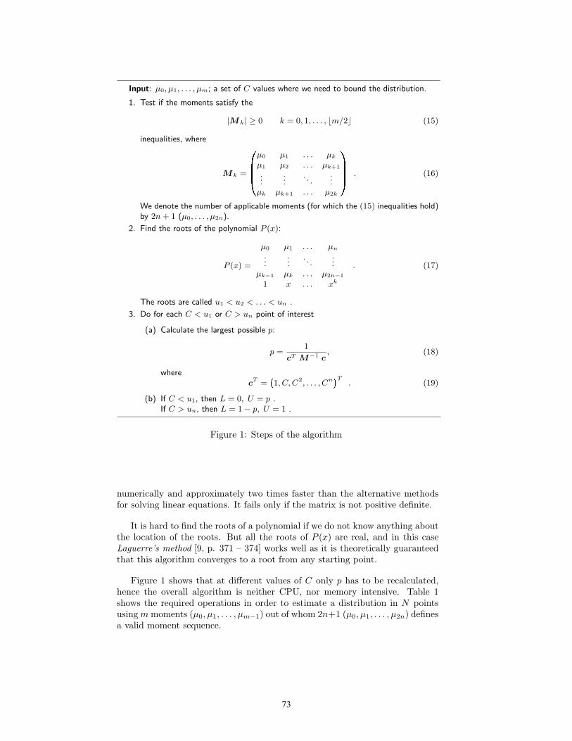
Input: µ0, µ1, . . . , µm; a set of C values where we need to bound the distribution.
1. Test if the moments satisfy the
|M k| ≥ 0 k = 0, 1, . . . , bm/2c (15)
inequalities, where
M k =
�����
µ0 µ1 . . . µk
µ1 µ2 . . . µk+1
......
. . ....
µk µk+1 . . . µ2k
����� . (16)
We denote the number of applicable moments (for which the (15) inequalities hold)by 2n + 1 (µ0, . . . , µ2n).
2. Find the roots of the polynomial P (x):
P (x) =
���������
µ0 µ1 . . . µn
......
. . ....
µk−1 µk . . . µ2n−1
1 x . . . xk
���������. (17)
The roots are called u1 < u2 < . . . < un .
3. Do for each C < u1 or C > un point of interest
(a) Calculate the largest possible p:
p =1
cT M−1
c, (18)
wherec
T = �1, C, C2, . . . , Cn�T
. (19)
(b) If C < u1, then L = 0, U = p .If C > un, then L = 1 − p, U = 1 .
Figure 1: Steps of the algorithm
numerically and approximately two times faster than the alternative methodsfor solving linear equations. It fails only if the matrix is not positive definite.
It is hard to find the roots of a polynomial if we do not know anything aboutthe location of the roots. But all the roots of P (x) are real, and in this caseLaguerre’s method [9, p. 371 – 374] works well as it is theoretically guaranteedthat this algorithm converges to a root from any starting point.
Figure 1 shows that at different values of C only p has to be recalculated,hence the overall algorithm is neither CPU, nor memory intensive. Table 1shows the required operations in order to estimate a distribution in N pointsusing m moments (µ0, µ1, . . . , µm−1) out of whom 2n+1 (µ0, µ1, . . . , µ2n) definesa valid moment sequence.
73

Task Nr. of executions
calculation of determinants bm/2c + 1finding n roots of P (x) 1inversion of an (n+1) × (n+1) matrix 1vector-matrix multiplications of size (n+1) × (n+1) 2Nscalar product of vectors of size (n+1) 2Nreciprocal 2N
Table 1: Computational cost of the simplified estimation
4 Closed-form expressions
The applicability of the simplified estimation depends on the smallest and thelargest root of P (x) . If the degree of the polynomial P (x) is less than 5, thenclosed form expressions can be deduced for ui, though for degrees 3 and 4 theseexpressions are much too complicated and would fill several pages.
However if the degree of P (x) is equal to 2 (hence we have 5 moments asinput: µ0, µ1, µ2, µ3 and µ4) the formulas for u1, u2 and even for p are quitesimple. Discrete construction is needed only in the interval [u1, u2].
u1,2 =µ1µ2 − µ0µ3 ±
√
−3µ21µ
22 + 4µ0µ3
2 + 4µ31µ3 − 6µ0µ1µ2µ3 + µ2
0µ23
2µ21 − 2µ0µ2
, (20)
1
p=
C4(µ21 − µ0µ2) + C3(−2µ1µ2 + 2µ0µ3) + C2(3µ2
2 − 2µ1µ3 − µ0µ4)+
µ32 + µ0µ2
3 + µ21µ4 − µ2(2µ1µ3 + µ0µ4)
+C(−2µ2µ3 + 2µ1µ4) + (µ23 − µ2µ4)
µ32 + µ0µ2
3 + µ21µ4 − µ2(2µ1µ3 + µ0µ4)
.
(21)
Having 3 input moments (µ0 = 1, µ1 and µ2) the discrete reference distri-bution contains only 1 point: C . The only root of P (x) and the maximalconcentrated mass at C are the following:
u1 = µ1, p =µ2 − µ2
1
C2 − 2Cµ1 + µ2
. (22)
The lower and upper bounding functions can be expressed by simple formulasalong the whole real axis.
L =
0 if C < µ1 ,(C − µ1)
2
C2 − 2Cµ1 + µ2
if C ≥ µ1 ,(23)
U =
µ2 − µ21
C2 − 2Cµ1 + µ2
if C < µ1 ,
1 if C ≥ µ1 .(24)
It is easy to see that L and U are continuous functions of C .
These formulas are simple but they make only rough estimations possible.The next section shows how the increasing number of moments affects accuracy.
74

1,0,0(-;-)
1,1,2(0.85;0.85)
1,2,2(0.6;0.6)
1,2,3(0.6;0.4)
1,1,3(0.66;0.66)
1,2,1(0.75;0.75)
1,2,0(1;-)
1,1,1(1;1)
1,1,0(1;-)
1,0,3(-;1)
1,0,2(-;1)
1,0,1(-;1)
λa
λa
λa
λa
λa
λa
λa
λa
λe
λe
λe
λe
λe
λe
λe
λe
λe
µa
µaµ
aµa
2µa
2µa
2µa
2µa
µe
2µe
3µe
µe
0.75µe
1.2µe
1.2µe
1.7µe
2µe
Figure 2: State space of the sample model
5 Example of application
This section demonstrates the properties of the proposed approach through anexample, pointing out its strengths and weaknesses.
[5] introduced a strategy to share a telecommunication link between differenttraffic classes to satisfy certain pre-defined Quality of Service (QoS) constraints.Three traffic classes are defined:
• rigid: require constant bandwidth (br) allocation;
• adaptive: characterized by peak (ba) and minimum bandwidth (bmina )
requirements, the actual bandwidth usage depends on the link utilization(for example a video stream with adaptive compression level, where qualitydegradation is allowed to a certain degree, but high delay variance in not);
• elastic: similar to the adaptive class regarding their bandwidth require-ments (be and bmin
e ), but they stay in the system until a given amountof data has been transmitted (for example an ftp-session, where transferrate changes are allowed, but data loss is not).
A Markov reward model (MRM) is used to describe system behavior. Thestates of the system are represented by a triple (nr, na, ne) which are the num-ber of active flows in the system belonging to the rigid, adaptive and elasticflows, respectively. The arrival rates are λr, λa, λe, and the departure rates areµr, µa, µe. µe is called the maximal departure rate of an elastic flow experiencedwhen maximal bandwidth is available, the actual departure rate is proportionalto the available bandwidth, which is a function of nr, na and ne. The transi-tion rates of the MRM are calculated from these rates, and the reward ratesassociated with each state are the actual bandwidth of the elastic class.
Figure 2 shows a portion of the state space in case of nr = 1 . The stateswhere the elastic flows do not get the maximal bandwidth are printed in grey.The numbers below the state identifiers indicate the actual bandwidth of theadaptive and elastic flows as a fraction of their peak bandwidth.
The performance measure of our interest is the distribution of the amountof time, T (ξ), required to transmit ξ amount of data by an elastic traffic flow.
75

We would like to ensure that the transmission completes before time t with avery high probability:
Pr (T (ξ) < t) > ε, (25)
where ε is a prescribed constant close to 1 (0.99, . . . , 0.99999). The amount ofdata is given and we are interested in the minimum value of t which means thatthe transfer of ξ amout of data will be finished during the interval [0, tmin) withprobability e.g. 0.9999 but this is not true for any t < tmin .
This investigation requires evaluation of the MRM. We compare two differentanalysis approaches:
1. the moment-based method in [15] with estimation based on the moments;
2. direct analysis of the distribution of the completion time: methods of Nabliand Sericola [8], De Souza e Silva and Gail [2], Donatiello and Grassi [4].
The algorithms were implemented by their original paper. We use a dual AMDOpteron 248 (2.2 GHz) system with 6 GB of RAM running Linux for computa-tions.
5.1 Correctness
To verify the procedures we evaluate a sample system with 105 states and calcu-late the whole distribution of the amount of transmitted data. The three directmethods result in the same values and the moments-based method gives realbounds as it is depicted in Figure 3. The more moments are given the tighterthe bounds are. It is also observable that convergence slows down with theincreasing number of moments. The bounds are the widest around the mean ofthe distribution. We are able to do the estimations with maximum 17 moments,because using more moments results in negative determinant while testing thenecessary condition of existence (4). This is due to numerical instabilities in theprocedure that calculates the determinant of a matrix.
0
0.2
0.4
0.6
0.8
1
0 5 10 15 20
prob
abili
ty
point of interest (C)
exact value17 moments15 moments13 moments11 moments
9 moments7 moments5 moments
Figure 3: Distribution of the transmission time of ξ amount of elastic data
76

Moments Valid from 0.9999 0.99999 0.999999
5 13.668 48.542 78.919 122.9667 19.760 33.093 43.244 55.7569 23.188 29.364 34.462 44.32411 25.071 28.268 31.472 34.96713 26.285 27.902 30.121 32.45115 27.129 27.818 29.486 31.14417 27.698 27.815 29.169 30.405
Exact 26.590 28.373 29.145
Table 2: Moments based bounding of the tail distribution
5.2 Numerical results
We evaluate and estimate tmin, i.e. the minimum of t that satisfies (25). Threevalues of ε are considered: 0.9999, 0.99999 and 0.999999, ξ is set to 100. Fig.4 shows the exact distribution and the bounds we get using different numberof moments in case of ε = 0.9999 . Thick black line represents this value.All the three direct analysis methods result the same values, the correspondingcurve is labeled “exact” and tmin is the point where it reaches 0.9999 . Whenestimating a distribution based on its moments we get a lower and an upperbounding function. In these special cases that we investigate the upper boundingfunction is always equal to 1 and that’s why it is omitted in the figure. Thelower estimation is always smaller than the real value in any point of interestC, hence all the lower bounding functions corresponding to different numberof moments are below the exact distribution function. As a consequence thesefunctions intersect the line 0.9999 at greater values of t than tmin .
0.9997
0.99975
0.9998
0.99985
0.9999
0.99995
1
25 30 35 40 45 50
prob
abili
ty
point of interest (C)
exact value17 moments15 moments13 moments11 moments
9 moments7 moments5 moments
Figure 4: Lower estimation reaches to 0.9999
Table 2 presents the experiences. The 3rd, 4th and 5th columns contain theresults at different values of accuracy ε . The last row contains the “Exact”values which result from the direct distribution analysis. The other rows show
77

the points where the moment-based estimation reaches the predefined level ofaccuracy. The “Valid from” column indicates un, i.e. from which the presentedsimple bounding method is applicable (see (13)) and no reference discrete dis-tribution is needed.
The table clearly shows that more moments contain more information aboutthe tail distribution, and the estimated value of tmin is closer to the real one inthese cases. However convergence slows down as the number of used momentsincreases.
5.3 Size of the state space
We evaluated a series of runs to determine the maximum number of stateswhich the different types of solvers are still capable to calculate. We considereda method unusable if it resulted in clearly invalid values (e.g., negative possibil-ities) or the running time was more than 20× of the previous configuration.
0.1
1
10
100
1000
10000
10 100 1000 10000 100000 1e+006
time
of c
ompu
tatio
n (s
)
number of states
momentsSilva
DonatielloSericola
Figure 5: Evaluation time vs. state space size in logarithmic scale
Using the moments based method we could calculate the model with 370,000states, while direct methods calculated the model with maximum 12,000 states.On the other hand the moments based approach yields less information aboutthe distribution. The evaluation time of the estimation from the moments is0.01s, its contribution to the overall calculation time in all considered cases isnegligible.
6 Conclusion
In this paper we focus on a special use of our previously developed momentsbased distribution bounding method. For the computation of the distributionof extreme events the moment based analysis simplifies, because the maximalprobability mass at the point of interest defines the bounds of the distribution.
We present an example where the simple bounding method is efficient andaccurate compared to the results of other methods that calculate directly the
78

values of the distribution function.We plan to increase the accuracy of our algorithm by using extended preci-
sion arithmetic and to improve our method using additional information aboutthe distribution functions such as finite support intervals.
References
[1] N. I. Akhiezer. The classical moment problem and some related questionsin analysis. Hafner publishing company, New York, 1965. (translationof N. I. Ahiezer: Klassiqeska� Problema Momentov i Nekoto-
rye Voprosy Analiza, published by Gosudarstvennoe Izdatel~stvo
Fiziko-Matematiqesko$i Literatury, Moscow, 1961).
[2] E. de Souza e Silva and H.R. Gail. Calculating cumulative operationaltime distributions of repairable computer systems. IEEE Transactions onComputers, C-35:322–332, 1986.
[3] E. de Souza e Silva and R. Gail. An algorithm to calculate transient dis-tributions of cummulative rate and impulse based reward. Commun. inStatist. – Stochastic Models, 14(3):509–536, 1998.
[4] L. Donatiello and V. Grassi. On evaluating the cumulative performancedistribution of fault-tolerant computer systems. IEEE Transactions onComputers, 1991.
[5] G. Fodor, S. Racz, and M. Telek. On providing blocking probability- andthroughput guarantees in a multi-service environment. International Jour-nal of Communication Systems, 15:4:257–285, May 2002.
[6] H. Hamburger. Uber eine Erweiterung des Stieltjes’schen Momentproblems.Mathematische Annalen, 81:235–319, 1920.
[7] G. Horvath, S. Racz, A. Tari, and M. Telek. Evaluation of reward analysismethods with MRMSolve 2.0. In 1st International Conference on Quan-titative Evaluation of Systems (QEST) 2004, pages 165–174, Twente, TheNetherlands, Sept 2004. IEEE CS Press.
[8] H. Nabli and B. Sericola. Performability analysis: a new algorithm. IEEETransactions on Computers, 45:491–494, 1996.
[9] W. H. Press, B. P. Flannery, S. A. Teukolsky, and W. T. Vetterling. Numer-ical Recipes in C: The Art of Scientific Computing. Cambridge UniversityPress, 1993. http://lib-www.lanl.gov/numerical/bookcpdf.html.
[10] S. Racz. Numerical analysis of communication systems through Markovreward models. PhD thesis, Technical University of Budapest, 2000.
[11] S. Racz, A. Tari, and M. Telek. A moments based distribution boundingmethod. 2005. to appear in Computers and mathematics with applications.
[12] S. Racz and M. Telek. Performability analysis of Markov reward modelswith rate and impulse reward. In M. Silva B. Plateau, W. Stewart, ed-itor, Int. Conf. on Numerical solution of Markov chains, pages 169–187,Zaragoza, Spain, 1999.
79

[13] J. A. Shohat and D. J. Tamarkin. The problem of moments. AmericalMathematical Society, Providence, Rhode Island, 1946. Mathematical sur-veys.
[14] G. Szego. Orthogonal polynomials. American Mathematical Society, Prov-idence, Rhode Island, 1939.
[15] M. Telek and S. Racz. Numerical analysis of large Markovian reward mod-els. Performance Evaluation, 36&37:95–114, Aug 1999.
[16] A. van de Liefvoort. The moment problem for continuous distributions.Technical report, University of Missouri, WP-CM-1990-02, Kansas City,1990.
80
A New End-to-End Traffic-Aware Routing for MANETs
R.S. Al-Qassas, M. Ould-Khaoua and L.M. Mackenzie
Department of Computing Science University of Glasgow
Glasgow G12 8RZ UK
Email: {raad, mohamed, lewis}@dcs.gla.ac.uk
Abstract. In MANETs, resources, such as power and channel bandwidth are often at premium, and therefore it is important to optimise their use as much as possible. Consequently, a traffic aware technique to distribute the load is very desirable in order to make good utilisation of nodes’ resources. Therefore a number of end-to-end traffic aware techniques have recently been proposed for reactive routing protocols to deal with this challenging issue. In this paper we contribute to this research effort by proposing a new load aware technique that can overcome the limitations of the existing methods. Results from an extensive comparative evaluation show that the new technique has superior performance over similar existing end-to-end techniques in terms of the achieved packet delivery ratio and delay.
Keywords: Ad hoc networks, routing protocol, traffic, load balancing, latency, throughput, ns-2 simulation.
1. Introduction
Mobile Ad hoc Network (MANET) is a collection of wireless mobile nodes that form a temporary network without the need of any infrastructure or centralized administration. In such an environment, it may be necessary for one mobile node to enlist the aid of others in forwarding a packet to its destination due to the limited propagation range of each mobile node’s wireless transmissions [1]. The communication in MANETs is peer-to-peer as the mobile nodes communicate directly with one another. In MANET resources like power and bandwidth are at premium and it is important to minimise the use of these resources.
The routing protocol in MANETs is responsible for establishing and maintaining paths between nodes in the network. The topology of a MANET may change
81
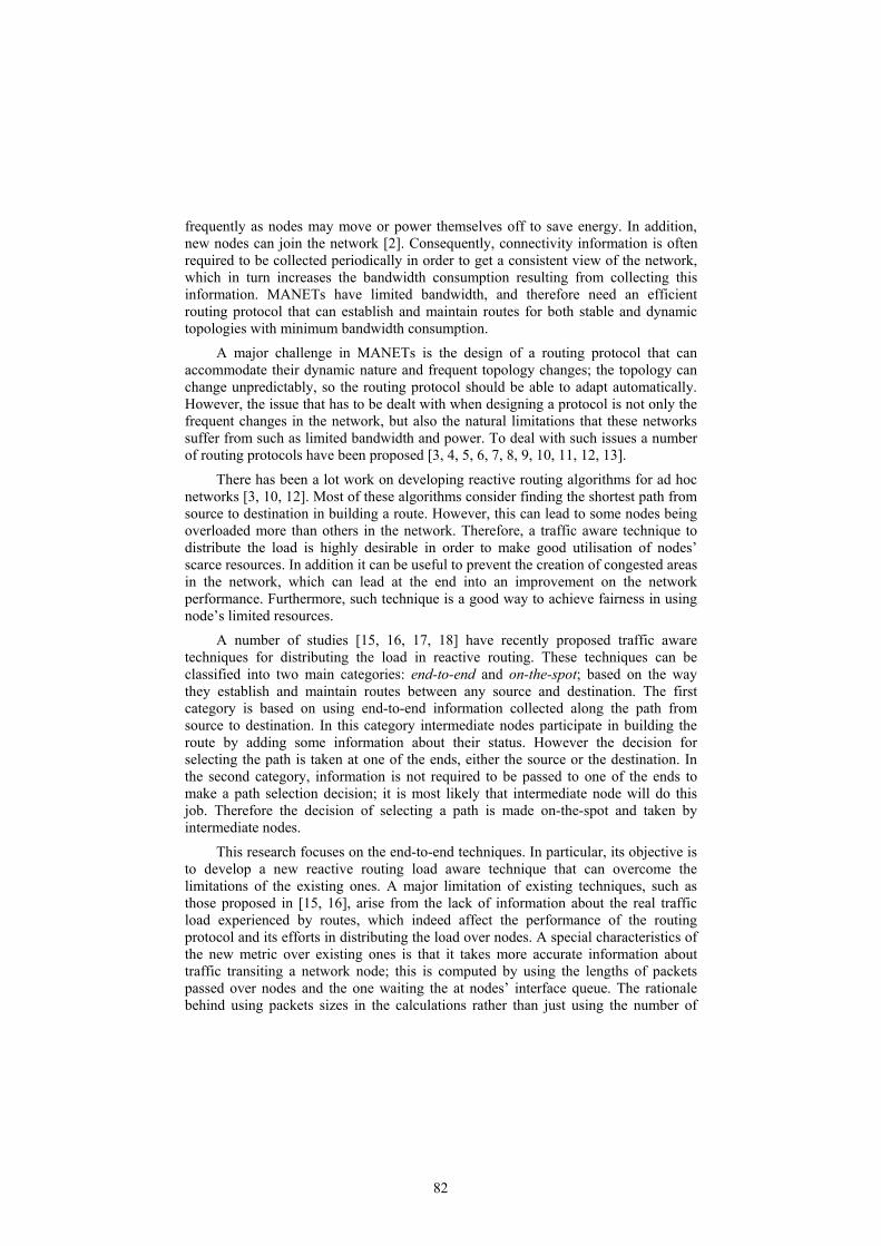
R.S. Al-Qassas, M. Ould-Khaoua and L.M. Mackenzie
frequently as nodes may move or power themselves off to save energy. In addition, new nodes can join the network [2]. Consequently, connectivity information is often required to be collected periodically in order to get a consistent view of the network, which in turn increases the bandwidth consumption resulting from collecting this information. MANETs have limited bandwidth, and therefore need an efficient routing protocol that can establish and maintain routes for both stable and dynamic topologies with minimum bandwidth consumption.
A major challenge in MANETs is the design of a routing protocol that can accommodate their dynamic nature and frequent topology changes; the topology can change unpredictably, so the routing protocol should be able to adapt automatically. However, the issue that has to be dealt with when designing a protocol is not only the frequent changes in the network, but also the natural limitations that these networks suffer from such as limited bandwidth and power. To deal with such issues a number of routing protocols have been proposed [3, 4, 5, 6, 7, 8, 9, 10, 11, 12, 13].
There has been a lot work on developing reactive routing algorithms for ad hoc networks [3, 10, 12]. Most of these algorithms consider finding the shortest path from source to destination in building a route. However, this can lead to some nodes being overloaded more than others in the network. Therefore, a traffic aware technique to distribute the load is highly desirable in order to make good utilisation of nodes’ scarce resources. In addition it can be useful to prevent the creation of congested areas in the network, which can lead at the end into an improvement on the network performance. Furthermore, such technique is a good way to achieve fairness in using node’s limited resources.
A number of studies [15, 16, 17, 18] have recently proposed traffic aware techniques for distributing the load in reactive routing. These techniques can be classified into two main categories: end-to-end and on-the-spot; based on the way they establish and maintain routes between any source and destination. The first category is based on using end-to-end information collected along the path from source to destination. In this category intermediate nodes participate in building the route by adding some information about their status. However the decision for selecting the path is taken at one of the ends, either the source or the destination. In the second category, information is not required to be passed to one of the ends to make a path selection decision; it is most likely that intermediate node will do this job. Therefore the decision of selecting a path is made on-the-spot and taken by intermediate nodes.
This research focuses on the end-to-end techniques. In particular, its objective is to develop a new reactive routing load aware technique that can overcome the limitations of the existing ones. A major limitation of existing techniques, such as those proposed in [15, 16], arise from the lack of information about the real traffic load experienced by routes, which indeed affect the performance of the routing protocol and its efforts in distributing the load over nodes. A special characteristics of the new metric over existing ones is that it takes more accurate information about traffic transiting a network node; this is computed by using the lengths of packets passed over nodes and the one waiting the at nodes’ interface queue. The rationale behind using packets sizes in the calculations rather than just using the number of
82

A New End-to-End Traffic-Aware Routing for MANETs
packets as in [15] is that packets can vary in size so it is better to use packets sizes as it can cover all the variations, and give a better indication of message contention. As a result, the new technique can potentially make a better judgment than the existing methods of [15, 16] in selecting routes, which improves the overall performance of the network, and distribute the load more fairly over the nodes in the network.
The remainder of this paper is organised as follows. Section 2 reviews two existing end-to-end techniques, namely degree of nodal activity and traffic density. Section 3 describes the proposed traffic aware technique. Section 4 conducts a comparative analysis of our proposed technique and the existing degree of nodal activity and traffic density techniques. Finally, section 5 concludes this study.
2. End-to-end traffic aware techniques
This section describes the end-to-end traffic aware techniques: degree of nodal activity suggested in the routing protocol “Load-Balanced Ad hoc Routing” (LBAR) [16] and traffic density suggested in “Load Aware Routing in Ad hoc” (LARA) [15].
2.1 Degree of nodal activity
The degree of nodal activity was defined in LBAR as a technique or metric for selecting the route with least traffic load. LBAR is a reactive routing protocol that focuses on how to find a path, which would reflect the least traffic load based on a cost function. The cost function is calculated using two components: nodal activity and traffic interference. Nodal activity of a node is defined as the number of active paths passing through that node. An active path is an established path from a source to a destination. Traffic interference is defined as the sum of nodal activity for the node’s immediate neighbours. The cost of a route is defined as the sum of nodes’ nodal activity plus the activity of their neighbouring nodes. The path with minimum cost is considered as the path with minimum traffic and is selected to be the path between source and destination.
Route discovery: In LBAR route discovery process is initiated whenever a source node needs to establish a path with another node. The source node broadcasts a setup messages to its neighbours. The setup message carries the cost seen from the source to the current node. A node that receives a setup message will forward it to its neighbours after updating the cost based on its nodal activity value and traffic interference value. In order to prevent looping when setup messages are routed, the setup message contains a list of all node IDs used in establishing the path from source node to the current intermediate node. The destination node collects arriving setup messages within a route-select waiting period, which is a predefined timer for selecting the best-cost path. After the waiting period expires the destinations sends an ACK message to the source node along the selected path. When the source node receives an ACK message,
83

R.S. Al-Qassas, M. Ould-Khaoua and L.M. Mackenzie
it recognises that a path has been established to the destination and then starts transmission.
Route maintenance: Route maintenance is triggered whenever a node on the active path moves out of the communication range, the case on which an alternate path must be found. If the source node moves away from the active path, the source has to reinitiate the route discovery procedure to establish a new route to the destination. When either the destination node or some intermediate node moves outside the active path, path maintenance will be initiated to correct the broken path. Once the next hop becomes unreachable, the node upstream of the broken hop propagates an error message to the destination node. The destination then picks up an alternative path and then sends an ACK message to the initiator of the error message. If the destination has no alternative path, it propagates an error message to the source, which will initiate a new route discovery if needed.
2.2 Traffic Density
The traffic density was proposed in LARA as a metric for selecting the route with the minimum traffic load. LARA uses traffic density to represent the degree of contention at the medium access control layer. This metric is used to select the route with the minimum traffic load when the route is setup. LARA protocol requires that each node maintain a record of the latest traffic queue estimations at each of its neighbours in a table called the neighbourhood table. Traffic queue is defined as the average value of the interface queue length measured over a period of time. Traffic density of a node is defined as the sum of traffic queue of that node plus the traffic queues of all its neighbours.
Route discovery: In LARA route discovery process is initiated whenever node needs to establish a path with another node. In the route request process, the source broadcasts a route request packet that contains a sequence number, a source id and a destination id. A node that receives the request, broadcasts the request further, after appending its own traffic density to the packet. This process continues until the request packet reaches the destination. After receiving the first request, the destination waits for a fixed time-interval for more route request packets to arrive. When the timer expires, the destination node selects the best route from among the candidate routes and sends a route reply to the source. When the source node receives the route reply, it can start data transmission. If it does not receive any route reply within a route discovery period, it can restart the route discovery procedure afresh.
Route maintenance: Route maintenance is triggered whenever a node on the active path moves out of the communication range, the case on which an alternate path must be found. If a link
84

A New End-to-End Traffic-Aware Routing for MANETs
failure occurs during a data transmission session, the source is informed of the failure via a route error packet. On receiving a route error packet, the source initiates a new route request and queues all subsequent packets for that destination until a new route is found.
3. The Proposed Load-density Metric
The existing end-to-end traffic aware techniques use a metric or cost function to select the route with a minimum load, such techniques are represented by nodal activity [16] and traffic density [15]. The nodal activity metric cost function calculation is based on monitoring the number of active paths passed over nodes. On the other hand, the traffic density metric is measured using number of packets at interface queue. However in order to make a good judgment about a given path’s load, it is not enough just to capture the number of active paths or number of packets at the interface queue over a period of time. Number of active paths can be useful when the used traffic flows are equal in characteristics. Number of packets at the interface queue is useful to capture the contention at the MAC layer if all packets are equal in size. However, this is not sufficient to represent the load. Therefore, what is needed is a metric that can deal with most of the cases that could appear in the network. Whether flows are with equal characteristics or not, or whether packets are equal in size or not, it should not affect the efficiency of the traffic aware technique. Our goal here is to devise a new end-to-end metric that selects the less congested route with the least traffic history regardless of the shape of the traffic passed over it.
Our proposed metric, named load-density, is calculated using two main components; the load history information represented by the total traffic passed over nodes, and the contention information represented by and the number of packets waiting at the nodes’ interface queue in order to take the possible contention in the network into consideration in the metric calculations. The load-density is embedded under a reactive routing algorithm like other existing metrics the degree of nodal activity and traffic density. The sections below describe this algorithm. As an alternative solution to represent the contention, we can use the sum of packets’ length occupying the queue as it can cover the variance in packets sizes instead of using the number of packets at interface queue.
Route discovery: The route discovery process starts whenever a node wants to communicate with another node for which it does not have a known route. The source node broadcasts a request packet to its neighbours. Every node receives the request packet will forward it to its neighbours after updating the cost information carried in the request packet, by adding the values of its load-history and contention information (see sec. 3.1) to the those carried in the packet. The cost information carried in the request packet, which includes the load history and the contention information, represents the cost seen from the source to the current node. The process of forwarding the request packet continues until the packet is received by the destination node. The destination
85

R.S. Al-Qassas, M. Ould-Khaoua and L.M. Mackenzie
collects the arriving request packets within a route selection period; activated upon receiving the first request packet, for selecting the best-cost route. Once the selection period is expired the destination selects the route with the best cost and sends a reply packet to the source node. The route selection process is illustrated in more details in Fig. 1.When the source node receives the reply packet, the path is then established and communication can be started.
// For selecting the route three parameters are used: // traffic load, contention information and path length in hops.
Collect all route requests packets sent from source S and received within the selection-period
// The selection-period is started when the first request packet is received. // Each request packet corresponds to a route from source to destination
Find the set of routes R that has contention value ≤ max-contention-threshold From the set R find the route r with minimum traffic-load
Compare the routes’ traffic-load with r’s traffic-load If the difference < acceptable-load-difference then select the route with the lowest number of hops and send reply to the source else select r as route and send reply to the source
If all routes available have contention values > max-contention-threshold then select the route with minimum traffic-load and send reply to the source
Fig. 1: Route selection algorithm in the new load aware metrics.
Route maintenance The route maintenance is triggered when there is a change in the topology that affects the validity of an active route. If the source node, an intermediate node or the destination node on an active route moves out of the communication range, an alternative route must be found. Once a node detects that the next hop is unreachable, it propagates an error message to the destination node. Upon receiving the error message, the destination node picks up an alternative route and then sends a reply message to the initiator of the error message. If the destination has no alternative path, it sends an error message to the source to start a route discovery process.
3.1 Route cost computation
The cost function has two main components: the data traffic load (in bytes) forwarded by nodes and number of packets at the interface queue. Every node keeps information about the amount of traffic passed over it during a predetermined period of time in the addition to the interface queue history represented by the averaged number of packets occupying the queue over a period of time. Route cost is calculated by gathering traffic load and contention information for the nodes along the route. The contention information for a node represents the number of packets at the interface queue plus the number of packets at the interface queue for its neighbours.
86

A New End-to-End Traffic-Aware Routing for MANETs
Nodes exchange contention information using hello packets. Each node broadcasts a hello packets every hello interval, to its neighbours, containing its identity and contention information. The hello packet is broadcasted only for one hop i.e. only to the immediate neighbours. Neighbours who receive this packet update their neighbourhood information.
4. Performance Evaluation
The performance comparison of the load-density metric against traffic density and nodal activity is carried out through extensive simulations implemented using the well-known network simulator ns-2 [14]. The simulation model we have used in the evaluation is illustrated in the sequel.
4.1. Simulation Model
The simulation model consists of the following main components: simulation area, simulation time, number of nodes, mobility model, maximum node speed, number of traffic flows, and traffic rate. Simulation model is represented by two scenario files, which are topology scenario and traffic scenario. The topology scenario corresponds to how nodes are distributed over the simulation area and there movement during the simulation time. The traffic scenario files contain the type of data, number of flows, traffic rate, and flow start time and end time. In all scenarios nodes are equipped with the wireless standard IEEE 802.11 with transmission range of 250m and a bandwidth of 2 Mbps.
In order to maximise the opportunity of forming multiple paths between data flow sources and their destinations we have chosen to make them stationary and the rest of the nodes in the network are mobile. The reason for this is that sources could become within the range of each other or very close due to mobility. Therefore keeping them stationary can boost our study of the traffic aware techniques.
We have implemented the traffic aware techniques load density, traffic density and nodal activity under AODV-like routing algorithm that is the AOMDV [19]. AOMDV is a multi-path algorithm that supports loop-free multiple paths. The ns-2 source code for this algorithm was available, and therefore it was easier to modify this source code to simulate the load density, traffic density and degree of nodal activity metrics rather than writing it from scratch.
4.2 Simulation Results
The evaluation is based on the simulation of 100 wireless nodes forming a MANET over a flat space of size (1200m × 1000m) for a period of 900 seconds. Flows with Constant Bit Rate (CBR) data have been used. The traffic rate varied between 2, 4 and 8 packets per second representing low, medium and high traffic loads, respectively. The numbers of CBR flows used are 3 and 5 flows with packet size of 512 bytes.
87

R.S. Al-Qassas, M. Ould-Khaoua and L.M. Mackenzie
Nodes move according to the random waypoint model [3] with a maximum speed of 10m/s. In random waypoint model each node remains stationary for a pause time period. The pause time has been varied from 0 to 900 seconds. When the pause time expires, the node selects a random destination in the simulation space and moves towards it. When the node reaches its destination, it pauses again for the same pause time. This behaviour is repeated throughout the simulation time. Simulation parameters are illustrated in Table 1.
Number of nodes 100 MAC layer IEEE 802.11 Transmission range 250m Simulation area 1200m x 1000m Simulation time 900s Mobility model Random waypoint model Maximum speed 10m/s Pause times 0, 150, 450, 900 Traffic type CBR Packet size 512 bytes Packet rate 2, 4, 8 Number of flows 3, 5
Table 1: The system parameters used in the simulation experiments
The performance of the three techniques is measured by: packet delivery ratio and end-to-end delay. The packet delivery ratio is the number of packets received at their final destinations over the total number of packets injected into the network. This measure provides an indication on the efficiency of a given routing protocol as it shows the amount of data packets that the protocol is able to deliver to destinations. End-to-end delay is the average time interval between the generation of a packet in a source node and the successful delivery of the packet at the destination node. It counts all possible delays that can occur in the source and all intermediate nodes.
Figures 2-7 depicts the delivery ratio for the three traffic aware techniques: load density, traffic density and nodal activity. Fig. 2 demonstrates the behaviour of the three techniques under 3 light traffic flows with a rate of 2 packets per second. The load density shows better delivery ratio compared to traffic density and nodal activity especially at pause time 0. Fig. 3 shows how the three techniques behave under medium traffic rate of 4 packets per second. The traffic density has higher delivery than nodal activity especially at low pause times. However, the load density outperforms the other techniques in all the simulated scenarios. Fig. 4 shows the performance of the three techniques under 3 high traffic flows with rate of 8 packets per second. Although the delivery ratio decreases compared to that in Fig. 3, our technique still outperforms the other techniques. In Fig. 5, the three methods exhibit comparable performance behaviour. However load density shows better performance than the other two techniques for all pause times. Figs. 6 and 7 illustrate how increasing the traffic rate would affect on the performance of the three methods. While the two methods; nodal activity and traffic density, have comparable performance under medium and high traffic rates, the load density method outperforms the other techniques in the simulated scenarios.
88

A New End-to-End Traffic-Aware Routing for MANETs
Figures 8-13 present the end-to-end delay for the three techniques. Fig. 8 shows delays when the traffic is light; 3 flows with a rate of 2 packets per second. The figure reveals lower delay for both the traffic density and load density techniques in most of the mobility conditions especially at pause time of 0 where high mobility conditions exist. The same behaviour is noticed under moderate traffic where 3 flows are used with a packet rate of 4 packets per second as it is shown in Fig. 9, except at 0 pause time where the load density is the one with better performance. In Fig. 10, although the three techniques show similar delays under high traffic rate of 8 packets per second, load density shows better performance than the other techniques.
Figures 11-13 shows the latency results under light, moderate as well as high traffic for 5 traffic flows with rates of 2, 4 and 8 packets per second, respectively. Fig. 11 shows that the load density technique with better performance than traffic density and nodal activity techniques under high mobility conditions, at 0 and 150 pause times. However the techniques have similar performance under low or no mobility conditions. Fig. 12 shows an increase in the end-to-end delay compared to that in Fig. 11. However load density has a lower packet delay, while the other techniques show close performance in most considered cases. Fig. 13, which depicts the behaviour of the techniques under high traffic, shows a great increase in the delay compared to that in figures 11 and 12. Although the techniques have similar performance, it is worth pointing out that the load density technique manages to achieve higher delivery ratios under the same operating conditions.
5. Conclusions
This study has suggested a new traffic aware technique, referred here to as load density that can overcome the limitations of the existing methods in reactive routing protocols. It has also conducted a performance evaluation of the new method against the two existing similar methods, notably, degree of nodal activity and traffic density under various working environments. Simulation results have revealed that in most circumstances the load density method exhibits superior performance in terms of both packet delivery ratios and end-to-end-delays. As a next step of this research, we plan to carry out further investigation on the performance of the techniques considering other working conditions by changing the node mobility pattern, traffic patterns, network size, and topological area.
References
[1] D.B. Johnson, Routing in Ad hoc Networks of Mobile Hosts, Proc. Workshop on Mobile Computing Systems and Applications, IEEE Computer Society, Santa Cruz, CA, December 1994 pp. 158-163.
[2] W. Chen, N. Jain and S. Singh, ANMP: Ad hoc Network Management Protocol, IEEE Journal on Selected Areas in Communications, Vol. 17, No. 8, August 1999, pp. 1506-1531.
89

R.S. Al-Qassas, M. Ould-Khaoua and L.M. Mackenzie
[3] D.B. Johnson and D.A. Maltz, Dynamic Source Routing in Ad Hoc Wireless Networks, In Mobile Computing, edited by T. Imielinski and H. Korth, Chapter 5, Kluwer Publishing Company, 1996, pp. 153-181.
[4] Z. Haas and M. Pearlman, The Performance of Query Control Schemes For the Zone Routing Protocol, IEEE/ACM Transactions on Networking (TON), Vol. 9, Issue 4, August 2001, pp. 427-438.
[5] C.E. Perkins and P. Bhagwat, Highly Dynamic Destination-Sequenced Distance Vector Routing (DSDV) for Mobile Computers, Proc. ACM SIGCOMM'94, London, September 1994, pp. 234-244.
[6] C.-C. Chiang, Routing in Clustered Multihop, Mobile Wireless Networks with Fading Channel, Proc. of IEEE SICON'97, April 1997, pp. 197-211.
[7] S. Murthy and J.J. Garcia-Luna-Aceves, An Efficient Routing Protocol for Wireless Networks, ACM Mobile Networks and Application, Special Issue on Routing in Mobile Communication Networks, Vol. 1, No. 2, October 1996, pp. 183-197.
[8] T. Clausen and P. Jacquet, Optimized Link State Routing Protocol, IETF MANET, Internet Draft, Jul. 2003.
[9] R. Ogier, F. Templin and M. Lewis, Topology Dissemination Based on Reverse-Path Forwarding (TBRPF), IETF MANET, Internet Draft, Oct. 2003.
[10] Y. Ko, N.H. Vaidya, Location-Aided Routing (LAR) in mobile ad hoc networks, Wireless Networks, Vol. 6, No. 4, 2000, pp. 307-321.
[11] C.-K. Toh, Associativity Based Routing For Ad Hoc Mobile Networks, Wireless Personal Communications Journal, Special Issue on Mobile Networking and Computing Systems, Vol. 4, No. 2, March 1997, pp.103-139.
[12] C.E. Perkins and E.M. Royer, Ad-hoc On-demand Distance Vector Routing, Proc. 2nd IEEE Workshop on Mobile Computing Systems and Applications, New Orleans, LA, Feb. 1999, pp. 90-100.
[13] V.D. Park and M.S. Corson, A Highly Adaptive Distributed Routing Algorithm for Mobile Wireless Networks, Proc. of IEEE INFOCOM '97, Kobe, Japan, April 1997, pp. 1405-1413.
[14] The Network Simulator ns-2, http://www.isi.edu/nsnam/ns. [15] V. Saigal, A.K. Nayak, S.K. Pradhan and R. Mall, Load balanced routing in mobile ad hoc
networks, Computer Communications, Vol. 27, Issue 3, Feb. 2004, pp. 295-305. [16] H. Hassanein and A. Zhou, Load-aware destination-controlled routing for MANETs ,
Computer Communications, Vol. 26, Issue 14, Sep. 2003, pp. 1551-1559. [17] S.B. Lee, Jiyoung Cho, and A.T. Campbell, A Hotspot Mitigation Protocol for Ad hoc
Networks, Ad hoc Networks Journal, Vol. 1, No. 1, March 2003. [18] M.R. Pearlman, Z.J. Haas, P. Sholander, and S.S. Tabrizi, On the impact of alternate path
routing for load balancing in mobile ad hoc networks, Proc. ACM MobiHoc, 2000, pp. 3-10.
[19] M. K. Marina and S. R. Das, On-demand Multipath Distance Vector Routing in Ad Hoc Networks, Proc. International Conference for Network Protocols (ICNP), Nov. 2001, pp. 14-23.
90

0.75
0.8
0.85
0.9
0.95
1
0 150 450 900
pause time (s)
Deliv
ery
ratio Traffic Density
Nodal activityLoad Density
Fig. 2: Packet delivery ratio for 3 flows of traffic with a rate of 2 packets/s.
0.75
0.8
0.85
0.9
0.95
1
0 150 450 900
pause time (s)
Deliv
ery
ratio Traffic Density
Nodal activityLoad Density
Fig. 3: Packet delivery ratio for 3 flows of traffic with a rate of 4 packets/s.
0.6
0.65
0.7
0.75
0.8
0.85
0.9
0.95
0 150 450 900
pause time (s)
Deliv
ery
ratio Traffic Density
Nodal activityLoad Density
Fig. 4: Packet delivery ratio for 3 flows of traffic with a rate of 8 packets/s.
0.75
0.8
0.85
0.9
0.95
1
0 150 450 900
pause time (s)
Del
iver
y ra
tio Traffic DensityNodal activityLoad Density
Fig. 5: Packet delivery ratio for 5 flows of traffic with a rate of 2 packets/s.
0.7
0.75
0.8
0.85
0.9
0.95
0 150 450 900
pause time (s)
Deliv
ery
ratio Traffic Density
Nodal activityLoad Density
Fig. 6: Packet delivery ratio for 5 flows of traffic with a rate of 4 packets/s.
0.4
0.45
0.5
0.55
0.6
0.65
0.7
0.75
0 150 450 900
pause time (s)De
liver
y ra
tio Traffic DensityNodal activityLoad Density
Fig. 7: Packet delivery ratio for 5 flows of traffic with a rate of 8 packets/s.
0
0.05
0.1
0.15
0.2
0 150 450 900
pause time (s)
dela
y (s
) Traffic DensityNodal activityLoad Density
Fig. 8: Packet delay for 3 flows of traffic with a rate of 2 packets/s.
0
0.05
0.1
0.15
0.2
0.25
0 150 450 900
pause time (s)
dela
y (s
) Traffic DensityNodal activityLoad Density
Fig. 9: Packet delay for 3 flows of traffic with a rate of 4 packets/s.
91

0.05
0.1
0.15
0.2
0 150 450 900
pause time (s)
dela
y (s
) Traffic DensityNodal activityLoad Density
Fig. 10: Packet delay for 3 flows of traffic with a rate of 8 packets/s.
0
0.02
0.04
0.06
0.08
0.1
0.12
0.14
0.16
0 150 450 900
pause time (s)
dela
y (s
) Traffic DensityNodal activityLoad Density
Fig. 11: Packet delay for 5 flows of traffic with a rate of 2 packets/s.
0
0.05
0.1
0.15
0.2
0.25
0 150 450 900
pause time (s)
dela
y (s
) Traffic DensityNodal activityLoad Density
Fig. 12: Packet delay for 5 flows of traffic with a rate of 4 packets/s.
0
0.05
0.1
0.15
0.2
0.25
0.3
0.35
0 150 450 900
pause time (s)
dela
y (s
) Traffic DensityNodal activityLoad Density
Fig. 13: Packet delay for 5 flows of traffic with a rate of 8 packets/s.
92

Effective Admission and Congestion Control for Interconnection Networks in Cluster Computing Systems
Shihang Yan, Geyong Min, and Irfan Awan
Department of Computing, School of Informatics, University of Bradford, Bradford, BD7 1DP, U.K.
{shyan, g.min, i.u.Awan} @brad.ac.uk
Abstract. Admission and congestion control mechanisms are integral parts of network design for providing Quality of Service (QoS) of real-world applications. The InfiniBand defines a System Area Networks (SANs) environment where multiple processor nodes and I/O devices are interconnected using a switched point-to-point fabric. InfiniBand is quickly becoming the interconnection of choice for cluster computing systems. This paper proposes an improved link-by-link based admission control mechanism and an effective source response function, named as Power Increase and Power Decrease (PIPD), for traffic congestion control. These proposed schemes adopt rate control to reduce congestion of multiple-class traffic in InfiniBand networks. Simulation experiments have demonstrated that the admission control algorithm and the new source response function are quite effective for the InfiniBand networks.
Keywords. InfiniBand, Congestion Control, Admission Control, ECN, PIPD.
1 Introduction
InfiniBand is quickly becoming the interconnection of choice for many high-performance computing systems, e.g., cluster systems, because of its compelling price/performance and standard-based technology [6]. InfiniBand Architecture (IBA) has been proposed as a new industry standard for high-speed I/O inter-processor communication. It is designed around a switch-based interconnection technology with high-speed point-to-point links [10] (see Fig. 1). The point-to-point interconnection means that every link in the IBA networks has exactly one device connected at each end of the link, thus providing better performance than traditional bus-shared architectures. InfiniBand switches were designed not only to enable large-scale server clusters but also to provide the ability to tie those clusters into Grid computing environments [3]. Because the InfiniBand-based interconnection provides the high bandwidth, low latency required by the Grid computing systems consisting of cluster applications, databases, shared network and storage resources. An IBA network is divided into subnets interconnected by routers, each subnet comprising one or more switches, processing nodes and I/O devices [2].
InfiniBand Architecture (IBA) has three mechanisms to support QoS: Service Level (SL), Virtual Lanes (VL), and Virtual Lane Arbitration (VLA) [1]. The switch in the InfiniBand networks consists of a crossbar where link and VL have dedicated access to the crossbar. Each link supports one or more VLs, each of which has its own buffer resources including an input buffer and an output buffer. Admission control algorithms help to meet the specific SL of the InfiniBand networks. However, admission control alone may not be effective enough to guarantee the QoS when the network operates under heavy traffic load. The overload can degrade the overall network performance seriously. Therefore, a congestion control mechanism should be used to monitor the network loads and intervene traffic actions when the loads reache a certain threshold indicating possible network congestion [19]. So both admission control and congestion control mechanisms are collectively required to guarantee various QoS constraints.
System Area Networks (SANs) provide high throughput and low latency for efficient I/O and cluster communication. The adoption of SANs has increased quickly in recent years and should accelerate with the emergence of industry standards such as InfiniBand [16]. InfiniBand can experience congestion spreading [4], where one bottleneck link causes traffic to be blocked throughout the network. The characteristics of IBA make the congestion control mechanism specifically challenging. Firstly, unlike traditional networks, InfiniBand switch cannot drop packets to deal with traffic congestion. Secondly, InfiniBand switches are single-
93
chip devices [10] with small packet buffers. So there are only a few packets in transit at any time. Thirdly, the latencies of switch and end-device processing are very low. For end-to-end congestion control in traditional networks, flow sources use packet dropping [11] or changes in network latencies [5, 13] as a signal of congestion. In this paper, we use the Explicit Congestion Notification (ECN) to detect congestion and notify the flow endpoint. ECN has been widely used in ATM networks [9] and Internet with TCP protocols [8, 14]. We adopt the ECN mechanism for InifniBand networks because the configuration of the switches with the input buffer is the same as that with output buffer in ATM networks. A source adjusts its packet injection rate after receiving congestion information. We propose a new source response function to improve the performance of the InfiniBand.
Fig. 1 IBA subnet: each subnet includes a set of switches and point-to-point links.
The major contributions of this paper are twofold: 1) to extend the traditional admission
control mechanism so that it is suitable to the InfiniBand architecture by considering different connections with various SLs in the networks subject to multiple-class traffic, 2) to propose a new effective source response function that can support the higher bandwidth utilization and ensure the fairness.
The rest of this paper is organized as follows: Section 2 presents an improved link-by-link based admission control mechanism. Section 3 describes the congestion control mechanism and source response function methodology. A new source response function will then be proposed. Section 4 uses simulation experiments to evaluate the effectiveness of our improved admission control mechanism and the new response function in an InfiniBand network subject to multiple-class traffic with different priorities. Finally Section 5 concludes this study and indicates future work.
2 Admission Control
This section will present the link-by-link based admission control mechanism with the proposed extension so that it is suitable to the InfiniBand architecture. In the link-by-link approach a bandwidth broker records the load on each link and consults the availability of the bandwidth before accepting or rejecting a new connection requirement. We adopt the approach described in [12] which ensures the sum of requested resources does not exceed link capacity. Let bw be the total link bandwidth, s the sum of bandwidth already admitted to existing connections, and p the bandwidth requested by the new potential connection. This algorithm accepts the new connection only the condition bwsp <+ is satisfied. In the
Processor Node CPU CPU
HCA
Processor Node CPU CPU
HCA
TCA Controller Storage
Switch
Switch
Switch Router
Processor Node CPU CPU
HCA
94

InfiniBand architecture, connections with different SLs have the different bandwidth requirements. Let
isls be the sum of the bandwidth that has been admitted to connections with
the SL isl . The connection is accepted only when ii slsl bwsp <+ is satisfied, where
islbw is the
effective bandwidth available to SL isl . The InfiniBand architecture defines a maximum of 16 SLs.
3 Congestion Control
This section will describe the congestion control mechanism for InfiniBand using an Explicit Congestion Notification (ECN) packet marking scheme and a source response function.
3.1 Packet marking
An alternative to implicit notification is ECN, in which switches detect incipient congestion and notify flow endpoints, for example, by marking packets when the occupancy of a switch buffer exceeds a desired operating point [15]. There is a single bit ECN field in the header of an identified packet that indicates the occurrence of congestion to the destination. The destination returns an acknowledgment packet (ACK) that includes the ECN value and the source will use this information to control the packet injection rate. We will extend the packet marking mechanism [16] that needs two counters for each output link. The first counter 1cnt records the current number of packets in the switch waiting for that output link. The second counter 2cnt records the number of subsequent packets that need to be marked when transmitted on that output ink. Whenever a buffer becomes full, the value of counter 1cnt is copied to counter 2cnt . This packet marking mechanism and descriptions of additional schemes are discussed in more detail in [17].
3.2 Source response function
The flow rate is adjusted in response to the feedback of network congestion. Because the feedback is received through the ACK packet, the flow injection rate will be adjusted whenever an ACK packet is received. If the receipt is an unmarked ACK, the source response must increase the flow rate. Similarly, if the receipt is a marked ACK, the source response must decrease the flow rate.
In order to design )(rfinc and )(rfdec , we use the condition defined in [16] as follows: Condtion1. Avoiding Congested State
The flows experience the same (or higher) degree of congestion after recovery. (1) ))(( rrff decinc ≤
Condition2. Fairness If the recover time )(rTrec for lower rate flows does not exceed that of higher flows, the
fairness is guaranteed.
)()( 21 rTrT recrec ≤ for 21 rr ≤ (2)
Condtion3. Efficiency In order to ensure the source response function efficient, the flows should recover rate
quickly to maximize bandwidth utilization.
min
11
)(R
rTrec = for maxmin1 )( RrRfdec ≤≤−
(3)
Some conclusions based on the conditions can be found in [16].
95

))(()( recincdecinc TtFftF += (4)
After an adjustment to rate r , the next ACK is received in a time interval r/1 , thus we get
)),/1(min()( maxRrFrf rincinc = (5)
In summary, to obtain an increase function )(rf inc we need to find a function )(tFinc that satisfies with Equation (4). In the next section, we will show how to obtain )(rf inc for a specific response function.
3.3 Power Increase Power Decrease (PIPD) function
Based on the unique characteristics, the source response function of the InfiniBand networks should be different from the current functions, such as the Additive Increase Multiplicative (AIMD) [7]. It is known that with the traditional increase function, such as the AIMD, the rate increase is the linear. Therefore, the injection rate can not reach a high speed quickly. The most bandwidth of the InfiniBand networks is under-utilized for a long time. So we consider using the power increase for the new function.
To design the increase function, we need to define a decrease function firstly, which uses the power function.
),max()( min/1 Rrrf mpipd
dec = where 1>m is constant. (6)
In order to avoid congested state from Equation (1), )(tFinc must satisfy the following
equation:
mincrecinc tFTtF )()( =+
(7)
This equation shows that after each interval time recT the function is powered by m . From this equation, we can get an obvious solution that an exponential function is based on the recT . For ...3,2,1 recrecrecrec TTTT ×××= and with min)0( RFinc = we get
recTtminc RtF
/
min)( = (8)
For any rate r , there exists a 't for which recTtm
inc RtFr/'
min)'( == . Therefore,
recrecTtrecTtm Ttinc
rinc rRttFrF /
min//'
)'()( ==+= +
(9)
In order to obtain the increase function )(tf inc form Equation (4),
)),/1(min()( maxRrFrf rinc
pipdinc =
),min( max
*/1min Rr
recTrR=
),min( max
/minRr
rRm= (10)
Noticing the increase function )(rfinc of PIPD, we can find that the change of the injection rate is based on the value of rR /min . Therefore, the PIPD mechanism can classify the different traffic priorities by giving them different value of minR . The increase function of PIPD make the injection increasing by power, unlike the linear increase function it can reach very high transmission rate in a short time.
Next we analyze how the PIPD function regulates the transmission rate in the InfiniBand networks. At the beginning, injection rate r is set to minR and the value of rR /min is equal to
96

1. The injection rate will increase very quickly because it is powered by m in fact. This can improve the utilization of the bandwidth. Then the injection rate is bigger than minR and the value of rR /min is less than 1, so the injection rate does not increase as fast as at the beginning. This will try to avoid congestion condition in the networks. From our analysis, the increase function of PIPD will not only control the rate well to suit the InfiniBand networks but also can improve the utilization of the bandwidth.
The decrease function also suits the InfiniBand networks environment. Because of small buffer size and the low network latency, the multiplicative decrease function cannot deal with the congestion in the InfiniBand networks. The power function decrease reduces the injection rate quickly enough to make the traffic flows relieve the congestion condition.
4 Simulation Scenarios and Performance Results
We have developed a discrete-event simulator to conduct a series of experimental study on the scenario illustrated in Fig. 2. Following [16], the network includes five endpoints and two switches A and B connected by a single physical link. The traffic flow generated at endpoint
1B and destined to endpoint cB ; we call it local flow as it is connected to the same switch of
the receiver. The traffic flow generated at endpoint 1A and destined to endpoint cB ; we call it remote flow because its packets need to be forwarded by switch A to switch B, through an inter switch link. A victim flow generated at endpoint vA and destined to endpoint vB through the inter-switch link between the two switches. Victim flow is destined to a non-congested endpoint vB and suffers from congestion spreading [16]. Table 1 lists the parameters used in our simulation.
Fig. 2 Simulation scenario
Table 1. Simulation Parameters
Parameters Value Link bandwidth 1GB/sec (InfiniBand 4X link) Packet header 20 bytes (InfiniBand Local Header) Data packet size 20 + 2048 = 2068 bytes Packet transmission time 2.068 sµ
Buffer size 8 packets
Our experiments test the performance of the improved link-by-link based admission control
mechanism and the new source response function PIPD. We assume there are two classes of traffic flows injected into each link with different SLs priorities and there is one remote flow and one local flow in the network. In the admission control stage, we set the bandwidth required by the high priority SL connection is two times of that required by the low priority SL connection. In the congestion stage, we set 128/maxmin RR high =− for the high priority flow
2r and 256/maxmin RR low =− for the low priority flow 1r with 4=m .
Switch B
Switch A
Av Bv
Bc
B1 A1
97
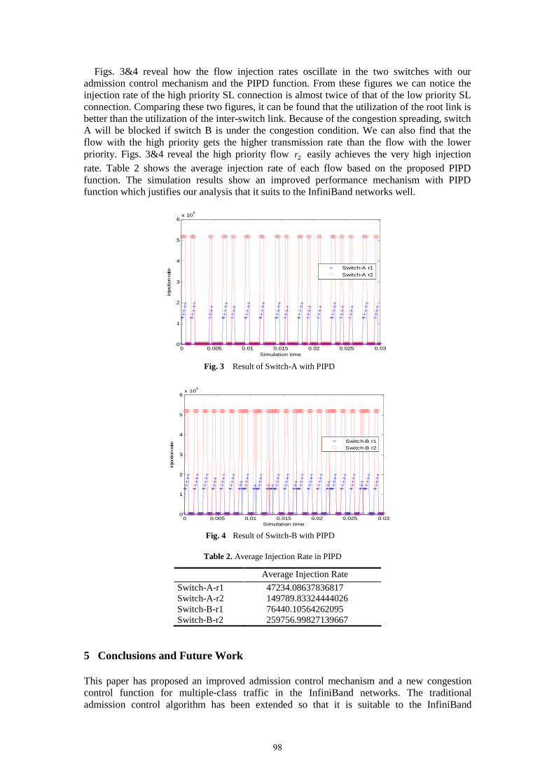
Figs. 3&4 reveal how the flow injection rates oscillate in the two switches with our admission control mechanism and the PIPD function. From these figures we can notice the injection rate of the high priority SL connection is almost twice of that of the low priority SL connection. Comparing these two figures, it can be found that the utilization of the root link is better than the utilization of the inter-switch link. Because of the congestion spreading, switch A will be blocked if switch B is under the congestion condition. We can also find that the flow with the high priority gets the higher transmission rate than the flow with the lower priority. Figs. 3&4 reveal the high priority flow 2r easily achieves the very high injection rate. Table 2 shows the average injection rate of each flow based on the proposed PIPD function. The simulation results show an improved performance mechanism with PIPD function which justifies our analysis that it suits to the InfiniBand networks well.
0 0.005 0.01 0.015 0.02 0.025 0.03
0
1
2
3
4
5
6x 10
5
Simulation time
inje
ctio
n ra
te
Switch-A r1
Switch-A r2
Fig. 3 Result of Switch-A with PIPD
0 0.005 0.01 0.015 0.02 0.025 0.03
0
1
2
3
4
5
6x 10
5
Simulation time
inje
ctio
n ra
te
Switch-B r1
Switch-B r2
Fig. 4 Result of Switch-B with PIPD
Table 2. Average Injection Rate in PIPD
5 Conclusions and Future Work
This paper has proposed an improved admission control mechanism and a new congestion control function for multiple-class traffic in the InfiniBand networks. The traditional admission control algorithm has been extended so that it is suitable to the InfiniBand
Average Injection Rate
Switch-A-r1 47234.08637836817 Switch-A-r2 149789.83324444026 Switch-B-r1 76440.10564262095 Switch-B-r2 259756.99827139667
98
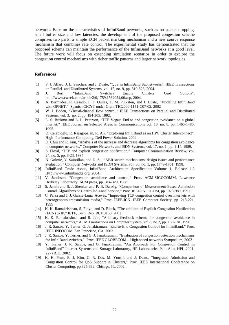
networks. Base on the characteristics of InfiniBand networks, such as no packet dropping, small buffer size and low latencies, the development of the proposed congestion scheme comprises two parts: a simple ECN packet marking mechanism and a new source response mechanism that combines rate control. The experimental study has demonstrated that the proposed schema can maintain the performance of the InfiniBand networks at a good level. The future work will focus on extending simulation scenarios in order to explore the congestion control mechanisms with richer traffic patterns and larger network topologies.
References
[1] F. J. Alfaro, J. L. Sanchez, and J. Duato, “QoS in InfiniBand Subnetworks” , IEEE Transactions on Parallel and Distributed Systems, vol. 15, no. 9, pp. 810-823, 2004.
[2] J. Burt, “ InfiniBand Switches Enable Clusters, Grid Options” , http://www.eweek.com/article2/0,1759,1562054,00.asp, 2004.
[3] A. Bermudez, R. Casado, F. J. Quiles, T. M. Pinkston, and J. Duato, “Modeling InfiniBand with OPNET,” Spanish CICYT under Grant TIC2000-1151-C07-02, 2002
[4] W. J. Boden, “Virtual-channel flow control,” IEEE Transactions on Parallel and Distributed Systems, vol. 3, no. 2, pp. 194-205, 1992.
[5] L. S. Brakmo and L. L. Peterson, “TCP Vegas: End to end congestion avoidance on a global internet,” IEEE Journal on Selected Areas in Communications vol. 13, no. 8, pp. 1465-1480, 1995.
[6] O. Celebioglu, R. Rajagopalan, R. Ali, “Exploring InfiniBand as an HPC Cluster Interconnect” , High- Performance Computing, Dell Power Solution, 2004.
[7] D. Chiu and R. Jain, “Analysis of the increase and decrease algorithms for congestion avoidance in computer networks,” Computer Networks and ISDN Systems, vol. 17, no. 1, pp. 1-14, 1989.
[8] S. Floyd, “TCP and explicit congestion notification,” Computer Communication Review, vol. 24, no. 5, pp. 8-23, 1994.
[9] N. Golmie, Y. Saintillan, and D. Su, “ABR switch mechanisms: design issues and performance evaluation,” Computer Networks and ISDN Systems, vol. 30, no. 1, pp. 1749-1761, 1998.
[10] InfiniBand Trade Assoc, InfiniBand Architecture Specification Volume 1, Release 1.2 Http://www.infinibandta.org, 2004.
[11] V. Jacobson, “Congestion avoidance and control,” Proc. ACM-SIGOCOMM, Lawrence Berkeley Laboratory, ACM press, pp. 314-329, 1988.
[12] S. Jamin and S. J. Shenker and P. B. Danzig, “Comparison of Measurement-Based Admission Control Algorithms or Controlled-Load Service,” Proc. IEEE-INFOCOM, pp. 973-980, 1997.
[13] C. Parsa and J. J. Garcia-Luna_Aceves, “ Improving TCP congestion control over internets with heterogeneous transmission media,” Proc. IEEE-ICN. IEEE Computer Society, pp. 213-221, 1999
[14] K. K. Ramakrishnan, S. Floyd, and D. Black, “The addition of Explicit Congestion Notification (ECN) to IP,” IETF, Tech. Rep. RCF 3168, 2001.
[15] K. K. Ramakrishnan and R. Jain, “A binary feedback scheme for congestion avoidance in computer networks,” ACM Transactions on Computer System, vol.8, no.2, pp. 158-181, 1990.
[16] J. R. Santos, Y. Turner, G. Janakiraman, “End-to-End Congestion Control for InfiniBand,” Proc. IEEE INFOCOM, San Francisco, CA, 2003.
[17] J. R. Santos, Y. Turner, and G. J. Janakiramam, “Evaluation of congestion detection mechanisms for InfiniBand switches,” Proc. IEEE GLOBECOM – High-speed networks Symposium, 2002
[18] Y. Turner, J. R. Santos, and G. Janakiraman, “An Approach For Congestion Control In InfiniBand” Internet Systems and Storage Laboratory, HP Laboratories Palo Alto, HPL-2001-227 (R.1), 2002.
[19] K. H. Yum, E. J. Kim, C. R. Das, M. Yousif, and J. Duato, "Integrated Admission and Congestion Control for QoS Support in Clusters," Proc. IEEE International Conference on Cluster Computing, pp.325-332, Chicago, IL, 2002.
99

100
Analysis of Active Queue Management under Two Classes of Traffic
Lan Wang, Geyong Min, Irfan Awan
Department of Computing, School of Informatics, University of Bradford, Bradford, BD7 1DP, UK
{lwang9,G.Min,I.U.Awan}@Bradford.ac.uk
Abstract - Active Queue Management (AQM) is an effective mechanism to support end-to-end traffic congestion control in network routers. Dropping packets before the queue reaches its maximum capacity is the main idea behind AQM. This paper develops an analytical model for a finite capacity queueing system with AQM mechanisms subject to two classes of traffic. The joint and marginal performance measures including the mean queue length, response time, system throughput, probability of packet losses and mean waiting time have been derived. The validity of the analytical results has been demonstrated through simulation experiences. The analytical model has been used to evaluate the performance of the queueing system with the AQM scheme subject to two classes of traffic.
1. Introduction
In very large networks with heavy traffic, sources compete for bandwidth and buffer space while being unaware of the current state of the system resources. This situation can easily lead to congestion even when the demand for resources does not exceed those available [9]. Consequently, system performance degrades seriously due to the increase of packet loss. In this context, congestion control mechanisms play important roles in effective network resource management.
End-to-end congestion control mechanisms are not sufficient to prevent congestion collapse in the Internet. Basically, there is a limit to how much control can be accomplished from the edges of the network. Therefore, intelligent congestion control mechanisms for FIFO-based or per-flow queue management [11] and scheduling mechanisms are required in the routers to complement the endpoint congestion avoidance mechanisms. Scheduling mechanisms determines the sequence of packets to be sent, while queue management algorithms control the queue length by dropping packets when necessary.
Buffer is an important resource in a router or switch. The larger buffer can absorb larger burst arrivals of packets but can tend to increase queueing delays as well. The traditional approach to buffering is to set a maximum limit on the amount of data that can be buffered. The buffer accepts each arriving packet until the queue space is exhausted and drops all subsequent arriving packets until some space becomes available in the queue. This mechanism is referred to as Tail Drop (TD) that is still the most popular mechanism in IP routers today owing to its robustness and simple implementation. However, “Lock-Out” and “Full Queues” [3] due to dropping packets only when the congestion has occurred are the main drawbacks of TD. The other two alternative queue disciplines, “Random drop on full” and “Drop front on full” , which is applied when the queue becomes full, can solve the “Lock-Out” problem but not “Full Queues” problem [3].
To overcome these problems and to provide low end-to-end delay along with high throughput, a widespread deployment of Active Queue Management (AQM) in routers has been recommended in the IETF publications [3]. To avoid the buffer maintaining a full status for a long time, AQM mechanism starts dropping packets before the queue is full in order to notify incipient stages of congestion. By keeping the average queue length small, AQM decreases the average delay, thus resulting in increased link utilisation by avoiding global synchronisation. Two important points in an AQM mechanism are when and how to drop packets. The former is mainly based on either the averaging queue length or the actual queue length. The latter is based on the threshold and dropping function. Both have a significant impact on the average delay, throughput and probability of packet loss. However, it is difficult to set values for the parameters of an AQM mechanism. For example, as the most popular AQM mechanism, Random Early Detection (RED) was initially described and analyzed in [4] with the anticipation to overcome the disadvantages of TD. There are five parameters in RED that can individually or cooperatively affect its performance. How to
101

set parameters for RED was discussed by Sally in 1993 [7] and 1997 [5] separately in detail. But it is hard to choose a set of these parameter values to balance the trade-off between various performance measures with different scenarios. As a result, most studies on RED are using the values introduced by Sally in 1997 [5]. In order to reflect the real variation of the queue, the instantaneous queue length is used to compare with the set thresholds and a linear function is adopted to drop packets.
Analysing the effects of an AQM mechanism on the aggregate traffic becomes more and more important. A simple simulation scenario where only four FTP sources were considered has shown that RED performs better than TD in [7]. But against to Sally and Van’s original motivation, the more scenarios are considered, the more disadvantages of RED appear. Based on the analysis of extensive experiments of aggregate traffic containing various categories of flows with different proportions, Martin et al [10] concluded that the harm of RED due to using the average queue size appears, especially when the average value is far away from the instantaneous queue size. The interaction between the averaging queue length and the sharp edge in the dropping function results in some pathology such as increasing the drop probability of the UDP flows and the number of consecutive losses. On the other hand, Mikket et al [4] studied the effect of RED on the performance of Web traffic using HTTP response time, a user-centric measure of performance, and found RED can not provide a fast response time for end-user as well. In [6], a modification to RED, named as Gentle-RED (GRED), was suggested to use a smoothly dropping function even when avg>=maxth but not the sharp edge in the dropping function as before. In [10], an extension of GRED, named GRED-I, was suggested to use an instantaneous queue length instead of the averaging queue length, one threshold and the dropping probability varies smoothly from 0 to 1 between the threshold and the queue size. The surprised result in [2, 6, 10] reveals that GRED-I performs better than both RED and GRED in terms of the aggregate throughput, UDP loss probability, queueing delay and number of consecutive losses. Compared to RED, GRED appears less advantageous than GRED-I because, for RED, the averaging strategy causes more negative effects than the cooperation of the average queue length and the sharp edge in the dropping function.
All existing studies [2, 4, 6, 7, 10] on the performance of AQM are based on software simulation. It is known that simulation is time-consuming and analytical model becomes a cost-effective alternative to simulation for evaluating system performance under different design spaces. With the aim to develop such a tool for investigating the performance of AQM and justifying the choice of different parameters, this study develops a new analytical queueing model for AQM mechanisms with two classes of traffic.
The rest of this paper is organized as follows. Section 2 describes a queueing system model with AQM mechanisms for two classes of traffic. The joint and marginal performance measures are presented in Section 3. The performance results are validated and analysed in Section 4. Finally, Section 5 concludes the study.
2. The Analytical Model
We consider two classes of traffic in a single-server queueing system using FIFO discipline. The arrival of each class k )2,1( =k follows a Poisson process with an average arrival rate kλ . The
service time of both classes is exponentially distributed with mean µ/1 . The system capacity is
L . As shown in Figure 1, the packets of class k will be dropped randomly based on a linear dropping function when the customer number in the system exceeds the threshold kth . The
maximum dropping probabilities of both classes, 1maxd and 2maxd , are 1.
102

The dropping process can be seen as a decrease of the arriving rate with the probability kid ,
where i represents the customer number in the system. A state transition rate diagram of the M/M/1/L queueing system with the AQM mechanism is shown in Figure 2.
The kid for each class k is given as follows.
��
���
≤≤−
<≤=
+−+− Li thd
thi d
thLthii
11max11
11
*)(1
0 1
1
1 (1)
��
���
≤≤−
<≤=
+−+− Li thd
thi d
thLthii
22max11
22
*)(1
0 1
2
2 (2)
Let ip , L i ≤≤0 represent the probability of each state in the state transition diagram.
According to the transition equilibrium between in-coming and out-coming streams of each state and Probability Theory, the following equations can be found.
���
���
�
+=
<≤++=++
=+
−−−
+−−−
122
111
1
1122
111
122
11
102201
10
)(
1 )()(
)(
LLLL
iiiiiii
pddp
Li ppddpdd
ppdd
λλµ
µλλµλλ
µλλ
(3)
Solving these equations, the probability can be expressed as:
���
�
���
�
�
≤≤×+
=
++
=
∏
� ∏−
=
=
−
=
Li1 )(
)(1
1
0
1
0
22
11
1
1
0
22
110
pdd
p
ddp
i
k
kki
L
i
i
k
kk
µλλ
µλλ
(4)
22
11
22λλ ×+× thth dd
211
12λλ +×−thd
21 λλ +
211
1λλ +×thd
21 λλ +
Threshold 2 Threshold 1
Figure 2: A state transition rate diagram
µ µ µ µ µ µ
0 th2 th1
L
th1
Threshold 1 L Customer No. in the System
Figure 1: Dropping Functions for Two Classes
dmax: 1
Dropping Probability
th2
Threshold 2
Dropping Function For Class Two
Dropping Function For Class One
22
111
1 λλ ×+× −− LL dd
103

3. Performance Analysis
In what follows, we will derive the joint system performance metrics including the mean queue
length ( L ), mean response time ( R ), system throughput ( T ), probability of packet losses ( P )
and the mean waiting time ( qW ) and relevant marginal performance metrics for each class of
traffic.
3.1 The joint performance measures
The joint mean queue length and throughput can be calculated using the same way as for the traditional M/M/1/L queueing system. Then the mean response time and the mean waiting time in the queue can be solved by Little’s Law. The packet loss probability consists of the probability of packet loss after the queue is full and that of packet dropped before the queue is full.
�=
×=L
ii ipL
0
)( (5)
�−
=×+××=×−=
1
02
21
10 )()1(
L
iiii ddppT λλµ (6)
T
LR = (7)
T
LW
qq = (8)
�= +
×−+×−×=
L
i
iii
ddpP
0 21
22
11 )1()1(
λλλλ
(9)
3.2 The marginal performance measures
For a system in the steady-state, the average arrival rate equals to its throughput. So the throughput of each class can be expressed as Eq. (10). In Eq. (11), the ratio of the instant arrival rate of class k ( 2,1=k ) to the total arrival rate 21 λλ + is the instant probability of loss packets
from class k . Because both classes of traffic are served identically, the average response time and the delay of each class can be derived using Eqs. (12) and (13) [8]. The delay of a packet from class k can be decomposed into two parts: the mean residual life due to the other packets found in service and the waiting time due to customers found in the queue upon its arrival. In an M/M/1/L queueing system, the mean residual life equals to the mean service time. The average response time consists of the delay and mean service time for the packet.
�−
=××=
1
0
L
ik
kii
k dpT λ (10)
�= +
×−×=
L
i
kki
ik d
pP0 21
)1(
λλλ
(11)
�
�
−
=+
−
=+
×+
+××+
=1
01
22
11
1
01
22
11
)(
)1
(
L
ii
ii
kki
L
ii
ii
kki
k
pdd
d
ip
dd
d
R
λλλ
µλλλ
(12)
�
�
−
=+
−
=+
×+
××+
=1
01
22
11
1
01
22
11
)(
)(
L
ii
ii
kki
L
ii
ii
kki
kq
pdd
d
ip
dd
d
W
λλλ
µλλλ
(13)
In order to calculate the probability distribution of the marginal queue length for each class, the probability that packets of each class stay in any position in the system should be calculated firstly. There are L positions in the system with the number being L�1 from server to the tail of the
104

queue. If a packet from class k is allocated in the position i )1( Li ≤≤ when it arrives in the
system, it will experience all the positions j before i , ij ≤ . In other words, the probability that
there is a packet from class k in the state j should be the summation of all the probabilities that
the packet arrives in the system and is allocated at position i , Lij ≤≤≤1 . From the transition
diagram above, the later probability can be calculated intuitively as 2
21
1 λλλ
×+××
×ii
kki
idd
dp
Lij ≤≤≤1 . So the probability that a packet from class k is in position i , noted as kim , can be
derived as:
�
�
−
−=
−
−= ×+×
××
=1
1
1
1 22
11
)(
L
ijj
L
ij jj
kkj
j
ki
p
dd
dp
mλλ
λ
2,11 =≤≤ kLi (14)
If the number of packets from class k is q , Lq ≤≤0 , then the number of aggregate packets in
the system should be not smaller than q . When the length of the system is l ql ≥ , there are qlC composition of two classes to make the length of class k be q . Furthermore, the probability
of each composition is different and can be calculated using kim . So the marginal probability
distribution of queue length for each class k , kqp can be derived as follows:
[ ]
[ ]���
�
���
�
�
≤≤��
��
�
��
��
�
�
��
�
��
�
�
��
�
�×
=��
��
�
��
��
�
�
��
�
��
�
�
��
�
�×+
=
� � ∏
� � ∏
=
−
=
−
=+
=
−
=
−
=+
L
ql
C
i
l
j
jijl
L
l
C
i
l
j
jijl
q
Lqmp
mpp
pql
ql
1
0q
1
0
1
0
,1
1
1
0
1
0
,10
1
ql
ql
A
A
(15)
[ ]
[ ]���
�
���
�
�
≤≤��
��
�
��
��
�
�
��
�
��
�
�
��
�
�×
=��
��
�
��
��
�
�
��
�
��
�
�
��
�
�×+
=
� � ∏
� � ∏
=
−
=
−
=+
=
−
=
−
=+
L
ql
C
i
l
j
jijl
L
l
C
i
l
j
jijl
q
Lqmp
qmpp
pql
ql
1
0
1
0
1
0
,1
1
1
0
1
0
,10
2
ql
ql
B
B
(16)
To represent kqp , two matrices j
iA and jiB are used to describe the possible compositions and
defined as:
( )( )
����
�
����
�
�
−==×���
�
�
���
�
�
==
==
=
×−
×
×
×
1,2,1;,2
;,2,1 111
0;,2,1 222
11
11ijL ii
ij i
j i
jiC
)(i
)(i-
iC
iC
ji
ji
��
��
��
j1)-(i
1)-(j1)-(i
ji
A�
A�
A (17)
( )( )
����
�
����
�
�
−==×���
�
�
���
�
�
==
==
=
×−
×
×
×
1,2,1;,2
;,2,1 222
0;,2,1 111
11
11ijL ii
ij i
j i
jiC
)(i
)(i-
iC
iC
ji
ji
��
��
��
j1)-(i
1)-(j1)-(i
ji
B �
B �
B (18)
105
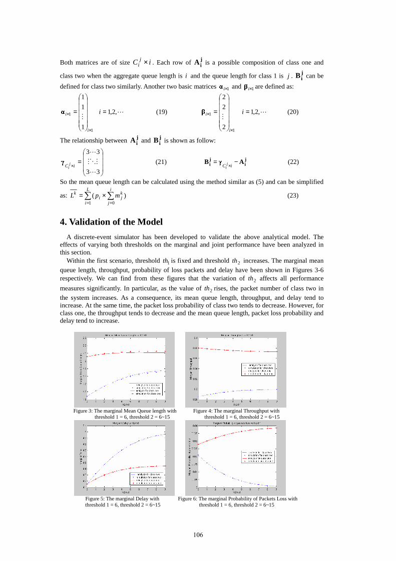
Both matrices are of size iC ji × . Each row of j
iA is a possible composition of class one and
class two when the aggregate queue length is i and the queue length for class 1 is j . jiB can be
defined for class two similarly. Another two basic matrices 1×i� and 1×i
�are defined as:
1
1
1
1
1
×
×
�����
�
�
�����
�
�
=
i
i�
� �,2,1=i (19)
1
1
2
2
2
×
×
�����
�
�
�����
�
�
=
i
i�
� �,2,1=i (20)
The relationship between jiA and j
iB is shown as follow:
���
�
�
���
�
�
=×
33
33
�
���
�
iC ji
� (21) ji
ji A�B −=
×iC ji
(22)
So the mean queue length can be calculated using the method similar as (5) and can be simplified
as: � �= =
×=L
i
i
j
kji
k mpL1 0
)( (23)
4. Validation of the Model
A discrete-event simulator has been developed to validate the above analytical model. The effects of varying both thresholds on the marginal and joint performance have been analyzed in this section.
Within the first scenario, threshold 1th is fixed and threshold 2th increases. The marginal mean
queue length, throughput, probability of loss packets and delay have been shown in Figures 3-6 respectively. We can find from these figures that the variation of 2th affects all performance
measures significantly. In particular, as the value of 2th rises, the packet number of class two in
the system increases. As a consequence, its mean queue length, throughput, and delay tend to increase. At the same time, the packet loss probability of class two tends to decrease. However, for class one, the throughput tends to decrease and the mean queue length, packet loss probability and delay tend to increase.
Figure 3: The marginal Mean Queue length with Figure 4: The marginal Throughput with threshold 1 = 6, threshold 2 = 6~15 threshold 1 = 6, threshold 2 = 6~15
Figure 5: The marginal Delay with Figure 6: The marginal Probability of Packets Loss with threshold 1 = 6, threshold 2 = 6~15 threshold 1 = 6, threshold 2 = 6~15
106
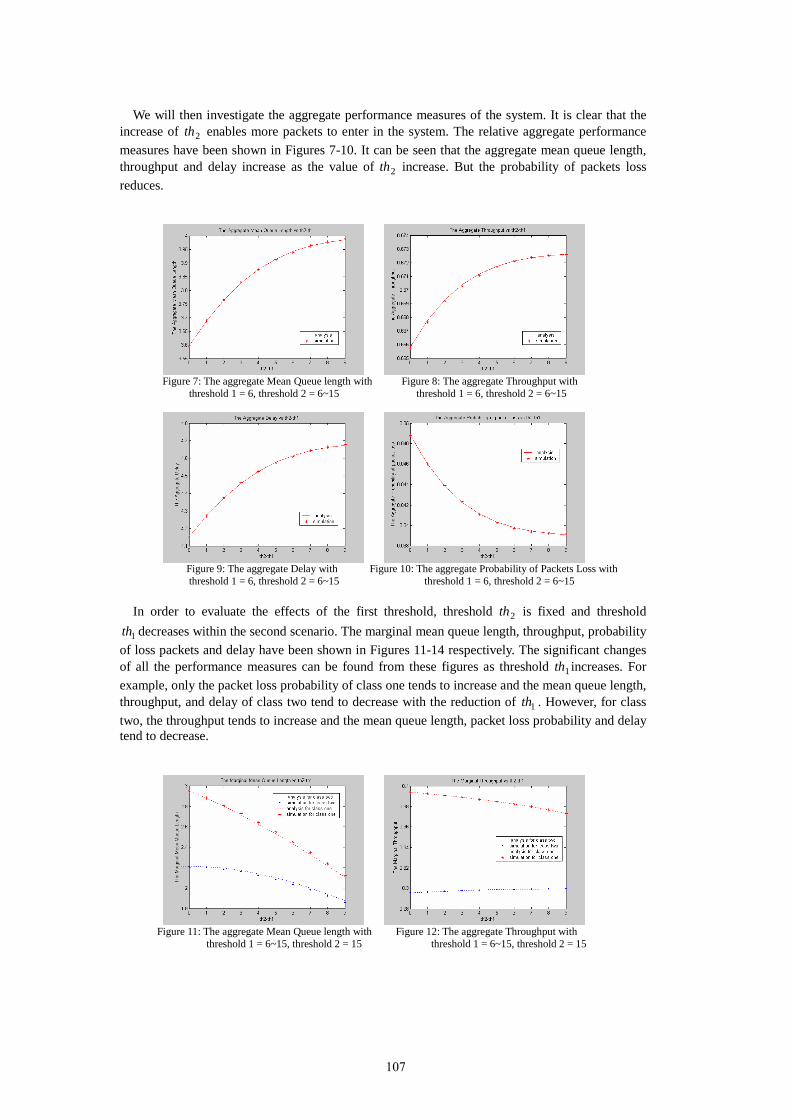
We will then investigate the aggregate performance measures of the system. It is clear that the
increase of 2th enables more packets to enter in the system. The relative aggregate performance
measures have been shown in Figures 7-10. It can be seen that the aggregate mean queue length, throughput and delay increase as the value of 2th increase. But the probability of packets loss
reduces.
Figure 7: The aggregate Mean Queue length with Figure 8: The aggregate Throughput with threshold 1 = 6, threshold 2 = 6~15 threshold 1 = 6, threshold 2 = 6~15
Figure 9: The aggregate Delay with Figure 10: The aggregate Probability of Packets Loss with threshold 1 = 6, threshold 2 = 6~15 threshold 1 = 6, threshold 2 = 6~15
In order to evaluate the effects of the first threshold, threshold 2th is fixed and threshold
1th decreases within the second scenario. The marginal mean queue length, throughput, probability
of loss packets and delay have been shown in Figures 11-14 respectively. The significant changes of all the performance measures can be found from these figures as threshold 1th increases. For
example, only the packet loss probability of class one tends to increase and the mean queue length, throughput, and delay of class two tend to decrease with the reduction of 1th . However, for class
two, the throughput tends to increase and the mean queue length, packet loss probability and delay tend to decrease.
Figure 11: The aggregate Mean Queue length with Figure 12: The aggregate Throughput with
threshold 1 = 6~15, threshold 2 = 15 threshold 1 = 6~15, threshold 2 = 15
107
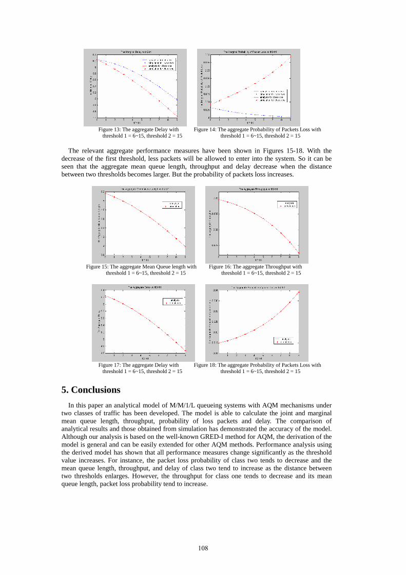
Figure 13: The aggregate Delay with Figure 14: The aggregate Probability of Packets Loss with threshold 1 = 6~15, threshold 2 = 15 threshold 1 = 6~15, threshold 2 = 15
The relevant aggregate performance measures have been shown in Figures 15-18. With the decrease of the first threshold, less packets will be allowed to enter into the system. So it can be seen that the aggregate mean queue length, throughput and delay decrease when the distance between two thresholds becomes larger. But the probability of packets loss increases.
Figure 15: The aggregate Mean Queue length with Figure 16: The aggregate Throughput with
threshold 1 = 6~15, threshold 2 = 15 threshold 1 = 6~15, threshold 2 = 15
Figure 17: The aggregate Delay with Figure 18: The aggregate Probability of Packets Loss with threshold 1 = 6~15, threshold 2 = 15 threshold 1 = 6~15, threshold 2 = 15
5. Conclusions
In this paper an analytical model of M/M/1/L queueing systems with AQM mechanisms under two classes of traffic has been developed. The model is able to calculate the joint and marginal mean queue length, throughput, probability of loss packets and delay. The comparison of analytical results and those obtained from simulation has demonstrated the accuracy of the model. Although our analysis is based on the well-known GRED-I method for AQM, the derivation of the model is general and can be easily extended for other AQM methods. Performance analysis using the derived model has shown that all performance measures change significantly as the threshold value increases. For instance, the packet loss probability of class two tends to decrease and the mean queue length, throughput, and delay of class two tend to increase as the distance between two thresholds enlarges. However, the throughput for class one tends to decrease and its mean queue length, packet loss probability tend to increase.
108

References [1] T. Bonald, M. May, J.C. Bolot, Analytic evaluation of RED performance, Proc.IEEE
INFOCOM, pp. 1415-1424, 2000. [2] C. Brandauer, G. Iannaccone, C. Diot, T. Ziegler, Comparison of tail drop and Active Queue
Management performance for bulk-date and Web-like Internet traffic, Proc. ISCC, pp. 122-129, 2001.
[3] B.Braden et al., Recommendations on queue management and congestion avoidance in the Internet, IETF RFC2039, 1998.
[4] M. Christiansen, K. Jeffay, D. Ott, F. Donelson Smith, Tuning RED for Web traffic, IEEE/ACM Trans. Network, vol 9, no. 3, pp. 249-264, 2001.
[5] S. Floyd, RED: discussions of setting parameters, http://www.icir.org/floyd/REDparameters.txt, 1997.
[6] S. Floyd, K. Fall, Promoting the Use of End-to-End Congestion Control in the Internet, IEEE/ACM Trans. Network, vol.7, no. 4, pp.485-472, 1999.
[7] S. Floyd, V. Jacobson, Random Early Detection gateways for congestion avoidance, IEEE/ACM Trans. Network, vol 1, no. 4, pp. 397-413, 1993.
[8] L.Kleinrock, Queueing Systems: Compute Applications, vol. 1, John Wiley & Sons, New York, 1975.
[9] D.E McDYSAN, QoS & Traffic Management in IP & ATM Networks, McGraw Hill, 1999. [10] M. May, C. Diot, B. Lyles, J. Bolot, Influence of Active Queue Management parameters on
aggregate Traffic Performance, INRIA.RR3995, 2000. [11] S.W. Ryu, C. Rump, C.M. Qiao, Advances in Internet congestion Control, IEEE
Communications survey, volume 5, no.1, 2003.
109

110
Performance Analysis of the LWQ QoS Model in MANETs
S. H. A. Wahab, M. Ould-Khaoua and S. Papanastasiou
Department of Computing Science
University of Glasgow Glasgow G12 8RZ
U.K. Email: {shaliza, mohamed, stelios}@dcs.gla.ac.uk
Abstract. Quality of Service (QoS) is essential in Mobile Ad Hoc Networks (MANETs) in order to satisfy communication constraints, e.g. delay, as set in real-time applications. Traffic from such applications is normally treated as high-priority in contrast to non delay sensitive applications such as FTP or e-mail, which are largely delay tolerant and have their flows treated as low-priority in the network. This paper analyses the performance behaviour of a recently proposed QoS model, notably LWQ, with respect to the number of high priority flows under a variety of mobility conditions. Our simulation results reveal that the number of high priority flows and different mobility states have a critical impact on the mean end-to-end delay and throughput of high priority traffic achieved by the LWQ QoS model.
Keywords: Mobile ad hoc networks, QoS, Delay, Throughput, High priority flows, Simulation.
1 Introduction MANETs [1] are formed by wireless devices that communicate with each other using multi-hop wireless links without necessarily using pre-existing network infrastructure. Two nodes communicate directly if they are in transmission range of each other or otherwise achieve connectivity through a multi-hop route via intermediate nodes. Hence, it becomes possible to establish spontaneous communication between network-enabled electronic devices. MANETs can also be formed by making use of other technologies such as optical networks, but wireless communications is the natural choice for spontaneous networking [2]. Advances in wireless communications and the growth of real-time applications such as streaming audio and games, have drawn a lot of attention to wireless networks that support quality of service (QoS). Due to limited availability of transmission bandwidth in MANETs, QoS techniques need to optimise the scarce resource by prioritising the real-time flows over best-effort flows in order to comply with the QoS requirement such as delay bounds and real-time throughput. Unlike best-effort applications, real-time applications require these QoS guarantees if they are to operate to a sufficient degree. Examples of applications are conversational voice, streaming, interactive and background/best-effort. The main distinguishing factor between these four classes lies with sensitivity to delay [3, 23]. In this research we have divided the real-time flows into two categories: delay-sensitive real-time flows and non delay-sensitive real-time flows. Delay-sensitive real-time flows are commonly considered as high priority and
111

non delay-sensitive real-time flows are considered low priority. As MANETs have been proposed for disaster relief environments, it is important to prioritise high priority flows so that an important flow will not be blocked due to existing low priority flows. Based on the above requirement, the goal of our research is to analyse an existing QoS model that deals with prioritisation. The reason we have chosen to analyse this model is because unlike existing models proposed in the literature [4, 5, 15], the LWQ model has a built-in mechanism that ensures tight QoS guarantees to high priority flows. We have performed extensive simulation experiments to investigate the performance behaviour of this model taking into account a number of important system parameters, including the number of high priority flows, node speed, pause time, and network size. The rest of the paper is organised as follows. In the next section, we briefly review several approaches and their extension for service differentiation. Section 3 provides a detailed description of the LWQ QoS model that we have analyzed. Section 4 evaluates the performance of LWQ in scenario of several competing high-priority flows. Finally, Section 5 concludes the findings and offers a plan for future work. 2 Existing QoS Approaches MANETs exhibit unique characteristics such as limited bandwidth availability and special mobility considerations. In order to guarantee QoS and given the limited bandwidth requirement it is necessary to prioritise certain flows over others; those high priority flows are then treated preferentially so as to meet given delay or throughput requirements. There exist several applications that need such type of treatment such as Voice over IP (VoIP). When the delay or the loss rate of such flows exceeds certain levels they become unusable. The existing approaches to QoS in MANETs satisfy some subset of these requirements [4, 5]. Some QoS solutions are built directly into existing routing [6, 7, 8, 9] or link layer protocols [10, 11, 12], making them completely dependant on the adoption of those protocols. Furthermore, several QoS approaches dealing with flow priority differentiation have been proposed in literature [13, 14,15]. The granularity of such differentiation is usually two-levels coarse, i.e. there are two types of flow: high and low priority. However, these priority differentiations have also been built into routing and link layer protocols. The SWAN model [16, 17], for instance, provides guarantees that are soft for high priority flows which implies that they may be downgraded to best-effort flows [18] in the presence of congestion.
One of the recently QoS model that attempts to provide tight guarantees to high priority flows is Light-weight QoS model (LWQ) [19, 20]. The following section describes the operation of the LWQ model and the limitations of its mechanism which has been the main motivation for our present study. 3 The operation of the LWQ model Light-weight QoS (LWQ) is a modified version of wired DiffServ QoS model [21] that takes into considerations the unique characteristics of multi-hop wireless environment. This model attempts to provide improved QoS to flows of highest priority class through a monitoring and correction mechanism which differentiates it with regard to other existing QoS models. As such, the packet rate of high priority flows is monitored
112
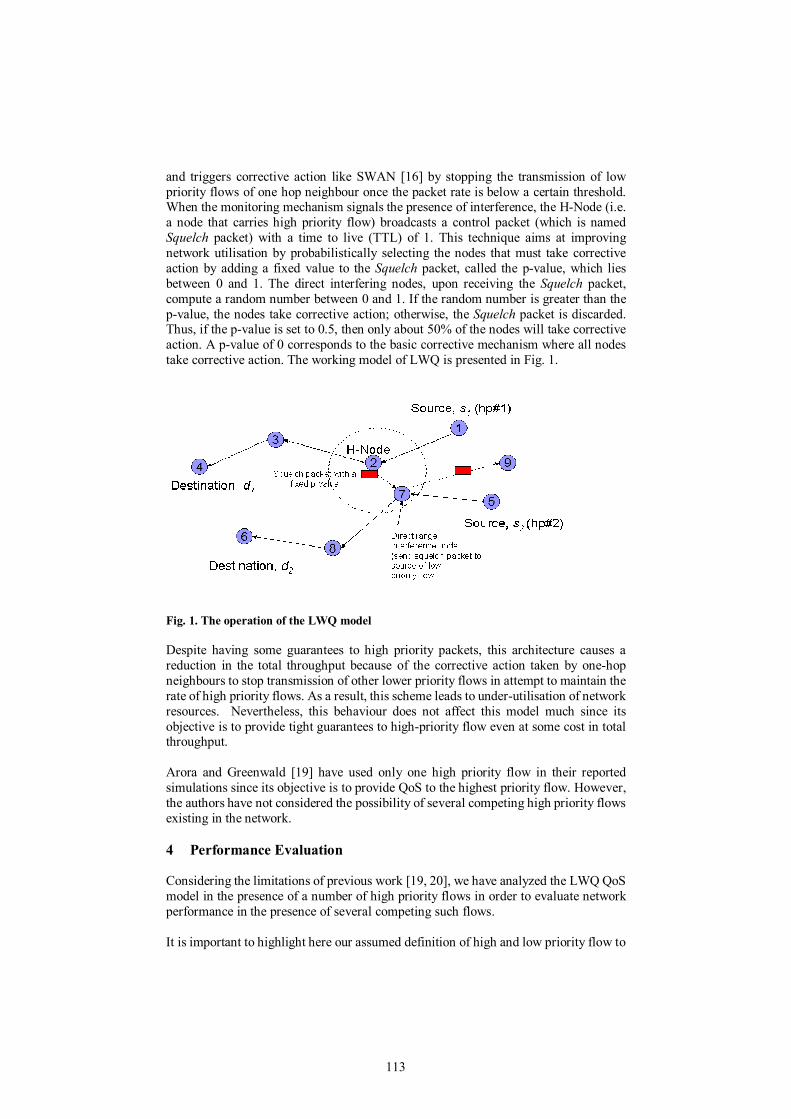
and triggers corrective action like SWAN [16] by stopping the transmission of low priority flows of one hop neighbour once the packet rate is below a certain threshold. When the monitoring mechanism signals the presence of interference, the H-Node (i.e. a node that carries high priority flow) broadcasts a control packet (which is named Squelch packet) with a time to live (TTL) of 1. This technique aims at improving network utilisation by probabilistically selecting the nodes that must take corrective action by adding a fixed value to the Squelch packet, called the p-value, which lies between 0 and 1. The direct interfering nodes, upon receiving the Squelch packet, compute a random number between 0 and 1. If the random number is greater than the p-value, the nodes take corrective action; otherwise, the Squelch packet is discarded. Thus, if the p-value is set to 0.5, then only about 50% of the nodes will take corrective action. A p-value of 0 corresponds to the basic corrective mechanism where all nodes take corrective action. The working model of LWQ is presented in Fig. 1.
Fig. 1. The operation of the LWQ model
Despite having some guarantees to high priority packets, this architecture causes a reduction in the total throughput because of the corrective action taken by one-hop neighbours to stop transmission of other lower priority flows in attempt to maintain the rate of high priority flows. As a result, this scheme leads to under-utilisation of network resources. Nevertheless, this behaviour does not affect this model much since its objective is to provide tight guarantees to high-priority flow even at some cost in total throughput. Arora and Greenwald [19] have used only one high priority flow in their reported simulations since its objective is to provide QoS to the highest priority flow. However, the authors have not considered the possibility of several competing high priority flows existing in the network. 4 Performance Evaluation Considering the limitations of previous work [19, 20], we have analyzed the LWQ QoS model in the presence of a number of high priority flows in order to evaluate network performance in the presence of several competing such flows. It is important to highlight here our assumed definition of high and low priority flow to
113

clarify our contribution in the context of previous work. We define high priority flows as 1) flows by delay-sensitive applications which require certain delay bound in order to operate properly and 2) flows that have high packet generation interval. As for low priority flows they are 1) non delay-sensitive application which do not require certain delay bound and 2) flows that have lower packet generation interval than the high priority flows. In order to perform a thorough analysis of this QoS model, we have considered the network topology and accompanying simulated traffic as indicated below: Network topology: describes the way the interconnection topology of nodes with different mobility affects the performance of the LWQ QoS model. Traffic: describes to the traffic load of high/low priority flows with different packet sending rate, packet length, and p-value of Squelch packet and in the way they affect the QoS requirement of high priority flows. We have used the network simulator ns-2 (v 2.26) [22] to run our experiments due to its extensive support for MANETs and ability to support QoS module such as DiffServ [21]. We have generated scenarios in a manner consistent with the recent LWQ architecture in [19] in which 50 nodes are considered, distributed over a 1500 x 300 m area and moving using Random Waypoint Model. Routing is handled by the AODV routing protocol which is mature routing solution in MANETs and a proposed RFC by the IETF. The channel bandwidth is 11 Mbps and the traffic sources are chosen to be constant bit rate (CBR) with background traffic of 3 to 5 low priority flows. Each simulation run lasts for 400 seconds in order to allow the network to experience some congestion. The offered load could be varied by changing the CBR packet size, the number of CBR flows or the CBR packet rate. In this experiment, we have fixed the CBR packet size and CBR packet rate but we have increased the number of high priority flows. When we increase the number of high priority flows, we decrease the number of low priority in order to maintain the same total number of running flows in the network. We set the rate of high priority flow to 32 80-byte packets per second so that it corresponds to audio streams of 20 Kbps and higher packet generation rate. The rate of low priority flow is 20 800-byte packets per second which in turn corresponds to multimedia on-demand retrieval application of 128 Kbps. The number of high priority flows is increased from 1 to 3 in our simulations. The number of low priority flows is decreased from 5 to 3 when we increase the number high priority flows in order to maintain the same amount of total high and low priority flows in the simulation. Several pairs of source and destinations of all flows are manually selected. Due to the similarities of the simulation results with different source-destination pairs, we only present the results from one representative simulation. The selected source-destination pair of three high priority flows are (1, 4), (5, 6) and (16,15) whereas the source-destination pair of low priority flows are (9, 10), (22, 45) and (7, 8). These pairs are selected to create multi-hop paths across the network. The simulation parameters and the traffic parameter of high priority flows and low priority flows are summarised in Table 1 and Table 2 respectively.
114

Table 1. The parameter for the LWQ model used in the simulations.
Simulation Parameter Value Number of nodes 50 Simulation area 1500 x 300 Maximum node speed 5, 10, 15, 20, 25 m/s Pause time 10s Simulation time 400s Routing protocol AODV MAC protocol IEEE 802.11
Table 2. The parameter of the generated traffic used in the simulations.
Traffic Value
Offered load 1 - 3 high priority flows, 3 - 5 low priority flows
Number of maximum high priority flows per node 2
Number of high priority flows 1, 2, 3 Source – destination pairs (s ,t) of high priority flows (1, 4), (5, 6) and (16, 15)
Start time for high priority flows 0, 1.0, 2.0 seconds respectively Packet length and packet interval 80 byte, 32 packets/second Rate of high priority packet 20 kbps Number of best-effort flows 5, 4, 3 Source – destination pairs (s, t) of low priority flows (9, 10), (22, 45) and (7, 8)
Start time for low priority flows 0.5, 1.5, 2.5 seconds respectively Packet length, packet interval 800 byte, 20 packets/sec Rate of low priority packet 128 kbps
We have evaluated the QoS model by comparing two performance metrics, namely: Mean end-to-end delay: is the time experienced by a packet between its initiation at the source and its reception at the destination. This is measured by the total packet delay of the flow per number of packets of the flow received at the destination. We have analysed the mean delay of high-priority packets since only high-priority flows is delay sensitive. High priority throughput: is the number of high priority packets received per unit time, expressed in percentage of number of packets received less than certain bounded delay. Any high priority packet received whose delay is greater than 100 ms will not be included in this high priority throughput calculation as in a real world implementation the application would have no use for it (it would be too late to be meaningful). Delay-sensitive applications, such as voice typically require an end-to-end delay of 400 ms for acceptable quality. However in order to evaluate this model for high priority voice applications, delay less than 100 ms is required; such a delay ensure lips synchronization [23] in video applications.
115

5 Results and Discussions This section presents the results for the mean end-to-end delay and high priority throughput considering different mobility conditions. Fig. 2 shows the impact of competing flows and mobility on mean end-to-end delay of each high priority flows as the number of high priority flows increases and at different mobility levels. Flow ID 1 to Flow ID 3 are high priority flows whereas Flow ID 4 to Flow ID 6 are low priority flows, The results show that the mean end-to-end delay is still maintained at less than 100 ms for two high priority flows (as indicated by bars beneath the dotted line of 0.1 s). However this delay requirement is violated when there are 3 high priority flows as the mean end-to-end delay of high priority flows increases drastically. This is a strong indication that the networks can only handle limited amount of high priority flows. As for low priority flows (Flow ID 4 to Flow ID 6), they also experience an increase in the mean end-to-end delay when there are 3 high priority flows. However this increase of the low priority flow delay is not significant enough to affect the application utilizing them since they are by definition resilient to delay changes.
Mean End-to-End Delay vs. Number of High Priority Flows
0.00.20.40.60.81.01.21.41.61.8
1hp
2hp
3hp
1hp
2hp
3hp
1hp
2hp
3hp
1hp
2hp
3hp
1hp
2hp
3hp
1hp
2hp
3hp
1 1 1 2 2 2 3 3 3 4 4 4 5 5 5 6 6 6
Number of high priority flows
Mea
n en
d-to
-end
del
ay (s
econ
ds)
5 m/s10 m/s15 m/s20 m/s25 m/s
Fig. 2. Mean end-to-end delay of high priority flows with increasing number of
high priority flows (grouped by Flow ID) at different mobility Fig. 3 shows the impact to delay of increasing the number of high priority flows under given mobility conditions. The throughput of high priority flows is calculated as the percentage of packets received within 100 milliseconds. The result shows that the throughput of high priority flows is maintained above 94% when there are up to two high priority flows. However this model starts to experience a throughput requirement violation when there are 3 high priority flows. In such a case, the throughput of the high priority flows decrease drastically. Similarly as with the results presented in Fig. 2, it is shown here that the network can only handle limited amount of high priority flows in order to maintain QoS guarantee.
High priority flows
100 ms
116
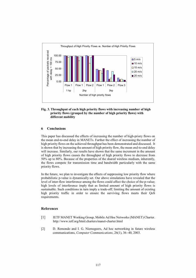
Throughput of High Priority Flows vs. Number of High Priority Flows
0.00
25.00
50.00
75.00
100.00
Flow 1 Flow 1 Flow 2 Flow 1 Flow 2 Flow 3
1 hp 2hp 3hp
Number of high priority flows
Per
cent
age
of p
acke
ts re
ceiv
edw
ith d
elay
< 1
00 m
s 5 m/s10 m/s15 m/s20 m/s25 m/s
Fig. 3. Throughput of each high priority flows with increasing number of high
priority flows (grouped by the number of high priority flows) with different mobility
6 Conclusions This paper has discussed the effects of increasing the number of high-priory flows on the mean end-to-end delay in MANETs. Further the effect of increasing the number of high priority flows on the achieved throughput has been demonstrated and discussed. It is shown that by increasing the amount of high priority flow, the mean end-to-end delay will increase. Similarly, our results have shown that the same increment in the amount of high priority flows causes the throughput of high priority flows to decrease from 50% up to 80%. Because of the properties of the shared wireless medium, inherently, the flows compete for transmission time and bandwidth particularly with the same priority flows. In the future, we plan to investigate the effects of suppressing low priority flow where probabilistic p-value is dynamically set. Our above simulations have revealed that the level of inter-flow interference among the flows could affect the choice of the p-value; high levels of interference imply that as limited amount of high priority flows is sustainable. Such conditions in turn imply a trade-off; limiting the amount of existing high priority traffic in order to ensure the surviving flows meets their QoS requirements. References [1] IETF MANET Working Group, Mobile Ad Hoc Networks (MANET) Charter.
http://www.ietf.org/html.charters/manet-charter.html [2] D. Remondo and I. G. Niemegeers, Ad hoc networking in future wireless
communications, Computer Communications, 26(1), 36–40, 2003.
117

[3] Nortel Networks white paper, Benefits of quality of service (QoS) in 3G
wireless internet, http://www.nortelnetworks.com, 2001. [4] G. -S. Ahn, A. T. Campbell, A. Veres, and L. -H. Sun. Supporting service
differentiation for real-time and best-effort traffic in stateless wireless ad hoc networks (SWAN), IEEE Transactions on Mobile Computing, 1(3): 192–207, 2002.
[5] S. -B. Lee, G. -S. Ahn, X. Zhang, and A. T. Campbell. INSIGNIA: An IP-based quality of service framework for mobile ad hoc networks, Journal of Parallel & Distributed Computing, 60(4): 374–406, 2000.
[6] Q. Xue and A. Ganz, Ad hoc QoS on-demand routing (AQOR) in mobile ad hoc networks, Journal of Parallel and Distributed Computing, 63(2): 154–165, February 2003.
[7] P. Sinha, R. Sivakumar and V. Bharghavan, CEDAR: A core extraction distributed ad hoc routing algorithm, IEEE Journal on Selected Areas in Communications, 17(8): 1454–1466, 1999.
[8] S. Chen and K. Nahrstedt, Distributed quality-of-service routing in ad hoc networks, IEEE Journal on Selected Areas in Communications, 17(8): 1488–1504, 1999.
[9] J. N. Al-Karaki, A. E. Kamal, Quality of service routing in mobile ad hoc networks: current and future trends, Mobile Computing Handbook, I. Mahgoub and M. Ilyas (eds.), CRC Publishers, 467–482, 2004.
[10] IEEE 802.11 WG, Draft Supplement to STANDARD FOR Telecommunications and Information Exchange Between Systems - LAN/MAN Specific Requirements - Part 11: Wireless Medium Access Control (MAC) and physical layer (PHY) specifications: Medium Access Control (MAC) Enhancements for Quality of Service (QoS), IEEE 802.11e/D2.0, Nov. 2001.
[11] P. Karn, MACA: A new channel access method for packet radio, in Proc. of ARRL/CRRL Amateur Radio 9th Computer Networking Conference, September 1990, 134–140.
[12] S. Kumar, V. S. Raghavan and J. Deng. Medium access control protocols for ad hoc wireless networks: a survey, Ad Hoc Networks, to appear, 2004.
[13] Y. Yang and R. Kravets. Throughput guarantees for multi-priority traffic in ad hoc networks, in IEEE International Conference on Mobile Ad Hoc Network and Sensor Systems, 2004, 379–388.
[14] X. Yang and N. Vaidya. Priority scheduling in wireless ad hoc networks, Proc.
of the 3rd ACM International Symposium on Mobile Ad Hoc Networking & Computing (MobiHoc '02), 2002, 71–79.
[15] G. -S. Ahn, Andrew T. Campbell, A. Veres, and L. -H. Sun. Supporting
service differentiation for real-time and best-effort traffic in stateless wireless ad hoc networks (Swan), IEEE Transactions on Mobile Computing, 1(3): 192–207, 2002.
118

[16] G. -S. Ahn, A. T. Campbell, A. Veres and L. -H. Sun, SWAN: Service
differentiation in stateless wireless ad hoc networks, Proc. 21st Annual Joint Conf. IEEE Computer Communication Societies(INFOCOM'2002), June 2002. 457–466.
[17] A. Veres, A. T. Campbell, M. Barry, and L. -H. Sun, Supporting service differentiation in wireless packet networks using distributed control, IEEE Journal of Selected Areas in Communications, Special Issue on Mobility and Resource Management in Next-Generation Wireless Systems, 19(10): 2081–2093, October 2001.
[18] Y. L. Morgan and T. Kunz, Enhancing swan QoS model by adopting destination-based regulation (ESWAN), Proc. Modeling and Optimization in Mobile, Ad Hoc and Wireless Networks (WiOpt’04), Mar. 2004. 112-121.
[19] H. Arora and L. Greenwald. Toward the use of local monitoring and network-wide correction to achieve QoS guarantees in mobile ad hoc networks, First Annual IEEE Communications Society Conference on Sensor and Ad Hoc Communications and Networks, (IEEE SECON 2004), Oct. 4–7. 2004, 128–138.
[20] H. Arora, Towards achieving QoS guarantees in mobile ad hoc networks, Masters Thesis, Drexel University, Department of Computer Science, Philadelphia, PA, November 2003.
[21] S. Blake, D. Black, M. Carlson, E. Davies, Z. Wang, W. Weiss, An
architecture for differentiated services, IETF RFC2475, December 1998. [22] The Network Simulator (NS-2). University of California, Berkeley.
http://www.isi.edu/nsnam/ns/
[23] N. Baghaei and R. Hunt, Review of quality of service performance in wireless LANs and 3G multimedia application services, Computer Communications, 27: 1684–1692, 2004.
119

120

Web Services Dependability and Performance Monitoring
Yuhui Chen1, Peter Li2 and Alexander Romanovsky1
1School of Computing Science, University of Newcastle upon Tyne, NE1 7RU, UK [email protected]
[email protected] 2School of Chemistry, University of Manchester, M60 1QD, UK
Abstract. The dependability of Web Services is becoming increasingly impor-tant for many application domains, such as e-Science, virtual organizations and service-oriented computing. The understanding of how a Web Service behaves in practice will help the developers to improve their service and provide clients with the information to determine the best ways of employing the Web Service. To fulfill such needs, we have developed a tool that monitors the dependability and performance of Web Services. The paper reports some initial results of the experiments in which the tool has been used.
1. Introduction
Dependability can be a major issue when using computational resources, for example,
during the enactment of a scientific workflow [1]. The reliability of service resources
can be erratic and this can lead to the failure of the workflow during its enactment [2].
The possibility of failure can be reduced by selecting those services which are the
most reliable based on data representing their behavioural characteristics. We have
developed a Java-based application which monitors the dependability of Web Ser-
vices. Users can set policies to constrain the tests, for instance, test interval, test pe-
riod and time out period. The tool collects this information from the Web Services
and displays real time statistics. It was used to investigate the reliability of two
BLAST Web Services from the bioinformatics domain. The performance characteris-
tics of the BLAST services were found to differ according to response time and com-
pletion status. It is hoped that this tool will enable users and client applications to
select those services which are the most reliable for their needs.
2. Overview of the Java tool
The tool measures the dependability of Web Services by acting as a client to the
Web Service under investigation. The tool monitors a given Web Service by tracking
the following reliability characteristics:
121

• Availability: The tool periodically makes dummy calls to the Web Service to
check whether it is running.
• Functionality: The tool makes calls to the Web Service and checks the re-
turned results to ensure the Web Service is functioning properly.
• Performance: The tool monitors the round-trip time of a call to the Web
Services producing and displaying real time statistics on service performance.
• Faults and exceptions: The tool logs faults and exceptions during the test
period of the Web Service for further analysis.
The tool can also test the dependability of a Web Service at geographically sepa-
rated locations on different Internet backbones through the deployment of the tool at
different physical locations. The tool and all information about it can be found at
http://www.students.ncl.ac.uk/yuhui.chen/
3. Comparison of BLAST Web Services
An experiment measuring the performance of two BLAST Web Services was un-
dertaken to test the monitoring tool. BLAST is an algorithm which is commonly used
in the bioinformatics domain to search for sequences that are similar to a given query
sequence [3]. However, the dependability of BLAST services can differ from one to
another. For a computationally-intensive in silico analytical experiment, it is impor-
tant that the most reliable services are used so that the chances of the experiment fail-
ing are reduced. To this end, the most reliable BLAST service can be judged based
on performance characteristics which have been measured by a tool such as that de-
scribed in this paper.
Performance metrics from two BLAST services were measured: a BLAST Web
Service1 deployed by the European Bioinformatics Institute (EBI), Cambridge, UK
and the BLAST service2 hosted by the DNA Database of Japan (DDBJ). Each
BLAST Web Service was invoked from three servers, two located in Newcastle upon
Tyne, UK and the other in China at 30 minute intervals for a period of 72 hours.
The response times of the EBI BLAST service varied dramatically during the 72
hour test period (Fig. 1A). The average response time of the service was ~900s. The
response time curves of from domestic broadband and University campus network in
Newcastle are similar, although the latter was slightly faster. The response time from
1 http://www.ebi.ac.uk/collab/mygrid/service4/soap/services/alignment::blastn_ncbi?wsdl 2 http://xml.nig.ac.jp/wsdl/Blast.wsdl
122
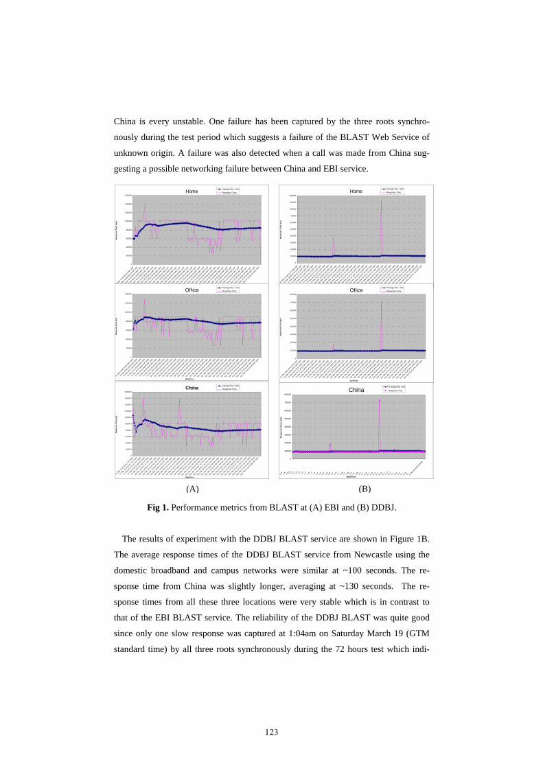
China is every unstable. One failure has been captured by the three roots synchro-
nously during the test period which suggests a failure of the BLAST Web Service of
unknown origin. A failure was also detected when a call was made from China sug-
gesting a possible networking failure between China and EBI service.
Fig 1. Performance metrics from BLAST at (A) EBI and (B) DDBJ.
The results of experiment with the DDBJ BLAST service are shown in Figure 1B.
The average response times of the DDBJ BLAST service from Newcastle using the
domestic broadband and campus networks were similar at ~100 seconds. The re-
sponse time from China was slightly longer, averaging at ~130 seconds. The re-
sponse times from all these three locations were very stable which is in contrast to
that of the EBI BLAST service. The reliability of the DDBJ BLAST was quite good
since only one slow response was captured at 1:04am on Saturday March 19 (GTM
standard time) by all three roots synchronously during the 72 hours test which indi-
Home
0
200000
400000
600000
800000
1000000
1200000
1400000
1600000
Fri Mar
18 06
:39:43
GMT 20
05
Fri Mar
18 08
:39:43
GMT 20
05
Fri Mar
18 10
:39:43
GMT 20
05
Fri Mar
18 12
:39:43
GMT 20
05
Fri Mar
18 14
:39:43
GMT 20
05
Fri Mar
18 16
:39:43
GMT 20
05
Fri Mar
18 18
:39:43
GMT 20
05
Fri Mar
18 20
:39:43
GMT 20
05
Fri Mar
18 22
:39:43
GMT 20
05
Sat Mar
19 00
:39:43
GMT 2
005
Sat Mar
19 02
:39:43
GMT 2
005
Sat Mar
19 04
:39:43
GMT 2
005
Sat Mar
19 06
:39:43
GMT 2
005
Sat Mar
19 08
:39:43
GMT 2
005
Sat Mar
19 10
:39:43
GMT 2
005
Sat Mar
19 12
:39:43
GMT 2
005
Sat Mar
19 14
:39:43
GMT 2
005
Sat Mar
19 16
:39:43
GMT 2
005
Sat Mar
19 18
:39:43
GMT 2
005
Sat Mar
19 20
:39:43
GMT 2
005
Sat Mar
19 22
:39:43
GMT 2
005
Sun M
ar 20
00:39
:43 G
MT 200
5
Sun M
ar 20
02:39
:45 G
MT 200
5
Sun M
ar 20
04:39
:45 G
MT 200
5
Sun M
ar 20
06:39
:45 G
MT 200
5
Sun M
ar 20
08:39
:45 G
MT 200
5
Sun M
ar 20
10:39
:45 G
MT 200
5
Sun M
ar 20
12:39
:45 G
MT 200
5
Sun M
ar 20
14:39
:45 G
MT 200
5
Sun M
ar 20
16:39
:45 G
MT 200
5
Sun M
ar 20
18:39
:45 G
MT 200
5
Sun M
ar 20
20:39
:45 G
MT 200
5
Sun M
ar 20
22:39
:45 G
MT 200
5
Data/Time
Res
pons
e Ti
me
(ms)
Average Res. timeResponse Time Home
0
100000
200000
300000
400000
500000
600000
700000
800000
900000
1000000
Fri Mar
18 06
:31:27
GMT 20
05
Fri Mar
18 08
:31:27
GMT 20
05
Fri Mar
18 10
:31:27
GMT 20
05
Fri Mar
18 12
:31:27
GMT 20
05
Fri Mar
18 14
:31:27
GMT 20
05
Fri Mar
18 16
:31:27
GMT 20
05
Fri Mar
18 18
:31:27
GMT 20
05
Fri Mar
18 20
:31:27
GMT 20
05
Fri Mar
18 22
:31:27
GMT 20
05
Sat Mar
19 00
:31:28
GMT 2
005
Sat Mar
19 02
:31:31
GMT 2
005
Sat Mar
19 04
:31:31
GMT 2
005
Sat Mar
19 06
:31:31
GMT 2
005
Sat Mar
19 08
:31:31
GMT 2
005
Sat Mar
19 10
:31:31
GMT 2
005
Sat Mar
19 12
:31:31
GMT 2
005
Sat Mar
19 14
:31:31
GMT 2
005
Sat Mar
19 16
:31:31
GMT 2
005
Sat Mar
19 18
:31:31
GMT 2
005
Sat Mar
19 20
:31:31
GMT 2
005
Sat Mar
19 22
:31:31
GMT 2
005
Sun M
ar 20
00:31
:31 G
MT 200
5
Sun M
ar 20
02:31
:32 G
MT 200
5
Sun M
ar 20
04:31
:32 G
MT 200
5
Sun M
ar 20
06:31
:32 G
MT 200
5
Sun M
ar 20
08:31
:32 G
MT 200
5
Sun M
ar 20
10:31
:32 G
MT 200
5
Sun M
ar 20
12:31
:32 G
MT 200
5
Sun M
ar 20
14:31
:32 G
MT 200
5
Sun M
ar 20
16:31
:32 G
MT 200
5
Sun M
ar 20
18:31
:32 G
MT 200
5
Sun M
ar 20
20:31
:32 G
MT 200
5
Sun M
ar 20
22:31
:32 G
MT 200
5
Data/Time
Res
pons
e Ti
me
(ms)
Average Res. timeResponse Time
Ofiice
0
100000
200000
300000
400000
500000
600000
700000
800000
Fri Mar
18 06
:34:57
GMT 20
05
Fri Mar
18 08
:34:57
GMT 20
05
Fri Mar
18 10
:34:57
GMT 20
05
Fri Mar
18 12
:34:57
GMT 20
05
Fri Mar
18 14
:34:57
GMT 20
05
Fri Mar
18 16
:34:57
GMT 20
05
Fri Mar
18 18
:34:57
GMT 20
05
Fri Mar
18 20
:34:57
GMT 20
05
Fri Mar
18 22
:34:57
GMT 20
05
Sat Mar
19 00
:34:57
GMT 2
005
Sat Mar
19 02
:34:57
GMT 2
005
Sat Mar
19 04
:34:57
GMT 2
005
Sat Mar
19 06
:34:57
GMT 2
005
Sat Mar
19 08
:34:57
GMT 2
005
Sat Mar
19 10
:34:57
GMT 2
005
Sat Mar
19 12
:34:57
GMT 2
005
Sat Mar
19 14
:34:57
GMT 2
005
Sat Mar
19 16
:34:57
GMT 2
005
Sat Mar
19 18
:34:57
GMT 2
005
Sat Mar
19 20
:34:57
GMT 2
005
Sat Mar
19 22
:34:57
GMT 2
005
Sun M
ar 20
00:34
:57 G
MT 200
5
Sun M
ar 20
02:34
:57 G
MT 200
5
Sun M
ar 20
04:34
:57 G
MT 200
5
Sun M
ar 20
06:34
:57 G
MT 200
5
Sun M
ar 20
08:34
:57 G
MT 200
5
Sun M
ar 20
10:34
:57 G
MT 200
5
Sun M
ar 20
12:34
:57 G
MT 200
5
Sun M
ar 20
14:34
:57 G
MT 200
5
Sun M
ar 20
16:34
:57 G
MT 200
5
Sun M
ar 20
18:34
:57 G
MT 200
5
Sun M
ar 20
20:34
:57 G
MT 200
5
Sun M
ar 20
22:34
:57 G
MT 200
5
Data/Time
Res
pons
e Ti
me
(ms)
Average Res. timeResponse Time
China
0
100000
200000
300000
400000
500000
600000
700000
800000
Data/Time
Res
pons
e Ti
me
(ms)
Average Res. time
Response Time
Office
0
200000
400000
600000
800000
1000000
1200000
1400000
Fri Mar
18 06
:43:29
GMT 20
05
Fri Mar
18 08
:43:29
GMT 20
05
Fri Mar
18 10
:43:29
GMT 20
05
Fri Mar
18 12
:43:29
GMT 20
05
Fri Mar
18 14
:43:29
GMT 20
05
Fri Mar
18 16
:43:29
GMT 20
05
Fri Mar
18 18
:43:29
GMT 20
05
Fri Mar
18 20
:43:29
GMT 20
05
Fri Mar
18 22
:43:29
GMT 20
05
Sat Mar
19 00
:43:29
GMT 2
005
Sat Mar
19 02
:43:29
GMT 2
005
Sat Mar
19 04
:43:29
GMT 2
005
Sat Mar
19 06
:43:29
GMT 2
005
Sat Mar
19 08
:43:29
GMT 2
005
Sat Mar
19 10
:43:29
GMT 2
005
Sat Mar
19 12
:43:29
GMT 2
005
Sat Mar
19 14
:43:29
GMT 2
005
Sat Mar
19 16
:43:29
GMT 2
005
Sat Mar
19 18
:43:29
GMT 2
005
Sat Mar
19 20
:43:29
GMT 2
005
Sat Mar
19 22
:43:29
GMT 2
005
Sun M
ar 20
00:43
:29 G
MT 200
5
Sun M
ar 20
02:43
:29 G
MT 200
5
Sun M
ar 20
04:43
:29 G
MT 200
5
Sun M
ar 20
06:43
:29 G
MT 200
5
Sun M
ar 20
08:43
:29 G
MT 200
5
Sun M
ar 20
10:43
:29 G
MT 200
5
Sun M
ar 20
12:43
:29 G
MT 200
5
Sun M
ar 20
14:43
:29 G
MT 200
5
Sun M
ar 20
16:43
:29 G
MT 200
5
Sun M
ar 20
18:43
:29 G
MT 200
5
Sun M
ar 20
20:43
:29 G
MT 200
5
Sun M
ar 20
22:43
:29 G
MT 200
5
Data/Time
Res
pons
e Ti
me
(ms)
Average Res. timeResponse Time
China
0
200000
400000
600000
800000
1000000
1200000
1400000
1600000
1800000
2000000
Fri Mar
18 14
:33:41
CST 2
005
Fri Mar
18 16
:37:47
CST 2
005
Fri Mar
18 18
:37:47
CST 2
005
Fri Mar
18 20
:37:48
CST 2
005
Fri Mar
18 22
:37:48
CST 2
005
Sat Mar
19 00
:37:47
CST 20
05
Sat Mar
19 02
:37:47
CST 20
05
Sat Mar
19 04
:37:46
CST 20
05
Sat Mar
19 06
:37:45
CST 20
05
Sat Mar
19 08
:37:45
CST 20
05
Sat Mar
19 10
:37:44
CST 20
05
Sat Mar
19 12
:37:44
CST 20
05
Sat Mar
19 14
:37:47
CST 20
05
Sat Mar
19 16
:37:46
CST 20
05
Sat Mar
19 18
:37:46
CST 20
05
Sat Mar
19 20
:37:45
CST 20
05
Sat Mar
19 22
:37:44
CST 20
05
Sun M
ar 20
00:37
:44 C
ST 2005
Sun M
ar 20
02:37
:43 C
ST 2005
Sun M
ar 20
04:37
:42 C
ST 2005
Sun M
ar 20
06:37
:41 C
ST 2005
Sun M
ar 20
08:37
:41 C
ST 2005
Sun M
ar 20
10:37
:40 C
ST 2005
Sun M
ar 20
12:37
:39 C
ST 2005
Sun M
ar 20
14:37
:39 C
ST 2005
Sun M
ar 20
16:37
:38 C
ST 2005
Sun M
ar 20
18:37
:38 C
ST 2005
Sun M
ar 20
20:37
:38 C
ST 2005
Sun M
ar 20
22:37
:37 C
ST 2005
Mon M
ar 21
00:37
:36 C
ST 2005
Mon M
ar 21
02:37
:36 C
ST 2005
Mon M
ar 21
04:37
:35 C
ST 2005
Mon M
ar 21
06:37
:35 C
ST 2005
Data/Time
Res
pons
e Ti
me
(ms)
Average Res. timeResponse Time
(A) (B)
123

cates an unknown Web service state. A timeout exception was also captured at
1:34am on Sunday March 20 (GTM standard time) by all three roots synchronously
indicating an unknown failure of the DDBJ BLAST Web Service.
4. Discussion and future work
The dependability of Web Services can vary according to a number of independent
internal and external factors. There are a number of solutions providing methods for
monitoring the use of Web Services. For example, the Bionanny Project [4] is devel-
oping a tool that can intercept requests incoming from clients, passing the requests to
the designated Web Service and measuring how many times the service is invoked
and how many different requests it receives. In effect, it acts as a proxy component to
the existing Web Services. However in order to develop dependable Web Services, it
is important to understand how the Web Services behave as clients. Our tool provides
measurements to fulfil this need. Since failures of Web Services can vary from inter-
nal faults to external errors, it is significant to understand where the faults are actually
deployed. The tool logs all exceptions for further investigation; however it is difficult
to understand some exceptions, especially those about timeout problems. It is planned
to improve the tool to have the ability to monitor and analyze the outgoing and incom-
ing SOAP messages to help discover the origin of service problems that have been
recorded.
Acknowledgements
We are grateful to Aad van Moorsel for several useful comments and suggestions.
References [1] Oinn T, Addis M, Ferris J, Marvin D, Greenwood M, Carver T, Senger M, Glover K, Wi-
pat A and Li P. Taverna: a tool for the composition and enactment of bioinformatics work-flows. Bioinformatics 20: 3045-3054. 2004.
[2] Stevens R, Tipney HJ, Wroe C, Oinn T, Senger M, Lord P, Goble CA, Brass A and Tassa-behji M. Exploring Williams-Beuren Syndrome Using myGrid. Bioinformatics 20: i303-i310. 2004.
[3] Altschul SF, Gish W, Miller W, Myers EW, Lipman DJ. Basic local alignment search tool. J Mol Biol. 215: 403-410. 1990.
[4] Senger M, Niemi M, Bionanny-A Web Service monitoring other Web Services. 2005. http://bionanny.sourceforge.net/
124

Predictive Run-time Adaptation for Service Level Agreements on the Grid
James Padgett, Karim Djemame and Peter Dew *
Abstract. Performance prediction of execution run-times is a key component when delivering timely application services in decision support systems. The provision of Service Level Agreements (SLA) and components to manage tasks such as resource negotiation, monitoring and policing are needed to help meet this requirement. This paper presents an SLA management architecture for use in Grid environments focusing on a policing strategy for Grid services. This includes a method for generating execution run-time predictions for tracking application progress. Experiments to test the prediction model are presented and show the prediction trace compared with a reference schedule.
Introduction
Grid computing [4] offers scientists and engineering communities access to high performance computational resources and applications. Within these virtual organisations users and resources often belong to multiple administrative domains. By definition, these resources are heterogeneous with varying quality and reliability. The ability to uphold commitments and assurances on top of the allocated resources is an application requirement, sometimes referred to as Quality of Service. A key goal of Grid computing is to deliver management on top of the allocated resources including availability of resources (compute resources, storage etc), security and network performance (latency, throughput) [7]. Commitments and assurances are implemented using Service Level Agreements (SLA), which determine a contract between a user and service provider, stating the expectations and obligations that exist between the two.
To support Grid systems based on timely service response a SLA management system incorporating resource reservation and run-time adaptation is desirable. In such systems there is a need for some form of resource monitoring and run-time adaptation on top of resource selection and reservation. An additional requirement is the provision of a historical record of the execution plan for auditing.
SLA management systems found in the literature [12, 21, 27] focus on a limited subset of management functions such as negotiation and reservation, or reservation and monitoring; few extend support for run-time adaptation. The approach presented here deals with these issues, but extends support for run-time adaptation including a system of warnings and notifications.
The paper presents a SLA management architecture for automated SLA negotiation, monitoring and policing mechanisms. The SLA Manager negotiates a SLA for the rights to execute a Grid application service using an external resource broker. Once an agreement exists, management of the SLA involves monitoring, which is achieved using performance measurement data obtained from a set of Grid monitoring tools. Policing is performed using violation data obtained through
* School of Computing, University of Leeds, {jamesp, karim, dew}@comp.leeds.ac.uk
125

automated monitoring of the SLA against real-time performance measurement data. Run-time adaptation is supported thanks to SLA policing mechanisms to enforce changes to the execution to meet SLA guarantees.
The aims of this paper are: firstly, to present a Grid SLA management architecture. Secondly, taking an SLA for a compute service as a motivation, discuss how a prediction model and rule based controller combine to provide predictive run-time adaptation for an application service. With this in mind, experiments are designed to test the performance of the prediction model and the rule based adaptation mechanism when the application service is executing on a large distributed Grid infrastructure, the White Rose Grid (WRG), which consists of high performance computing resources at Leeds, Sheffield and York Universities [29]. An infrastructure such as the WRG exhibits heterogeneous resources and spans multiple administrative domains.
SLA Architecture
The SLA Manager provides SLA and resource management support to virtual organisations such as the Distributed Aircraft Maintenance Environment (DAME) Diagnostic Portal [2]. In this example the SLA Manager is supporting a Grid based decision support system where timely and reliable service provision is a requirement. The user gains access to application services with the option of attaching time / performance constraints. The architecture is illustrated in Figure 1 and highlights component responsibilities.
Instantiation and Modification The SLA Factory provides a template for SLA specification based on user identification of relevant time or performance constraints. Additionally, the factory records provenance data within the SLA Instance during the policing phase. This provides a record of warnings and violations important for auditing after the agreement has terminated. Warnings are recorded when significant events are detected which may affect the SLA in the future but no actual violation has occurred. Violations are recorded when actual breaches in time or performance constraints have occured.
Negotiation and Reservation In order to fulfil a time or performance constraint the SLA Manager is able to negotiate for resources using a Resource Broker which has responsibility for placing reservations with a resource provider. The architecture allows for a community of brokers providing reservations for resources of different types, e.g. compute, storage and even bandwidth. The example used in this research is a SNAP-based resource broker [10], which provides reservations for compute resources. During the negotiation phase the user specifies a Task Service Level Agreement (TSLA), representing an agreement specification for a desired level of performance or time constraint for the Grid application service. Negotiation follows a request() / agree() protocol similar to that specified within the SNAP framework [6]. The SLA Manager enters into an agreement with the Resource Broker which provides a reservation guarantee, a Resource Service Level Agreement (RSLA), with the resource provider. Together the TSLA and RSLA form a Binding Service Level Agreement (BSLA) which binds the task to the potential resource capabilities promised in the RSLA.
126
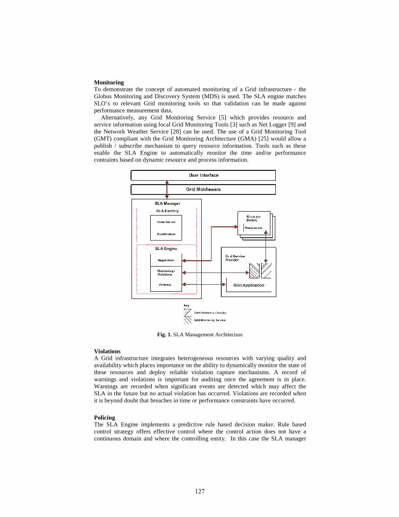
Monitoring To demonstrate the concept of automated monitoring of a Grid infrastructure - the Globus Monitoring and Discovery System (MDS) is used. The SLA engine matches SLO’s to relevant Grid monitoring tools so that validation can be made against performance measurement data.
Alternatively, any Grid Monitoring Service [5] which provides resource and service information using local Grid Monitoring Tools [3] such as Net Logger [9] and the Network Weather Service [28] can be used. The use of a Grid Monitoring Tool (GMT) compliant with the Grid Monitoring Architecture (GMA) [25] would allow a publish / subscribe mechanism to query resource information. Tools such as these enable the SLA Engine to automatically monitor the time and/or performance contraints based on dynamic resource and process information.
Fig. 1. SLA Management Architecture
Violations A Grid infrastructure integrates heterogeneous resources with varying quality and availability which places importance on the ability to dynamically monitor the state of these resources and deploy reliable violation capture mechanisms. A record of warnings and violations is important for auditing once the agreement is in place. Warnings are recorded when significant events are detected which may affect the SLA in the future but no actual violation has occurred. Violations are recorded when it is beyond doubt that breaches in time or performance constraints have occurred.
Policing The SLA Engine implements a predictive rule based decision maker. Rule based control strategy offers effective control where the control action does not have a continuous domain and where the controlling entity. In this case the SLA manager
127

does not have authoritative control over all applications submitted to the Grid infrastructure. In the first case the ability to effect the CPU processing potential is implemented either by migration onto a faster machine or one offering a load average which is less than that of the current resource. The adaptive process involves a prediction model, a rule based decision maker and a grid monitoring service. The decision maker takes input from two sources, the constraints stated in the SLA and the predicted remaining execution time generated by the predictive model.
Adaptation has the potential to significantly improve the performance and timely behaviour of an application bound with SLAs. Such an application can change its behaviour depending on available resources, optimising itself to its environment.
Prediction Model
The prediction model assumes the user has a reasonable approximation of the application execution time prior to submission. With this assumption the model provides a run-time assessment of the remaining execution time based on the CPU load immediately prior to and during application run-time. Assessments are made as to whether the application will complete within a specified time through comparison with the scheduled remaining execution time, which is agreed upon in the SLA during negotiation. Even when no approximation can be made, monitoring techniques can determine with some accuracy that the execution will take significantly longer than anticipated. In this situation the SLO cannot be expressed as a time constraint and another metric should be chosen. A good choice is a request to maintain a specified percentage of mean CPU usage for the application during run-time.
The fractional CPU usage iF is measured over n samples at time iT . %100T is the
time the task would take to execute if 100% CPU usage was maintained throughout application run-time. Festimate is the mean CPU usage over n samples.
estimate
n
iii
remaining F
FTTT
�−
=
∆−=
1
1%100
(1)
�=
==n
iinestimate F
nFF
1
1
(2)
Tremaining (1) is the predicted remaining execution time if Festimate (2) is maintained for the remainder of the execution. If Fi drops for a large proportion of this period the prediction will be invalid, subsequently, a new prediction is needed.
Experiments and Performance Results
Experiments are designed to test the policing phase of an application execution which operates in collaboration with the monitoring phase but after instantiation and negotiation is complete. Negotiation and monitoring have been the subject of previous study in [20] and [19]. When an SLA bound application is executing and a competing
128

appilication is submitted, the resource may no longer be able to meet its RSLA and subseqently the time or performance constraint in the TSLA may be violated.
Experiments are conducted on a large distributed Grid infrastructure; the WRG [29]. Once a SLA has been specified, the objective is to test the ability of the prediction model to generate reliable performance predictions for the remaining application execution time. The scenario uses a Grid application service used within the DAME project [2].
The prediction model assumes that the user knows a priori how long the application will take at 100% CPU usage. With this in mind the application service is executed at 100% CPU usage to determine a reference execution time. Once this is known the application service is executed from start to finish. During the course of the execution the predicted remaining execution time is generated periodically using the prediction model and is compared with the reference remaining execution time. This experiment is used to determine the accuracy of the RTP formula (1).
Prior to the experiment the application was run and took 1800 secs to complete with a mean CPU usage of 98%, resulting in a value of 1764 secs for T100%. As a result Tsla was set at a reasonable 2100 secs.
0
5
10
15
20
25
30
1 3 5 7 9 11 13 15 17 19 21 23 25 27 29
Actual Time Remaining (minutes)
Pre
dic
ted
Tim
e R
emai
nin
g (
min
ute
s)
Fig. 2. Predicted time remaining vs. actual time remaining
The results in Figure 2 show the prediction model provides a good match with the reference remaining execution time suggesting that the model is accurate and can be used for the remaining experiments.
Following this, additional applications are submitted to the same resource to disrupt the SLA bound application. This creates a violation in the time constraint Tsla and initiates control actions as defined in the rule base. This is compared to the case where no adaptive technique is used. It is used to determine the effectiveness of the rule-based decision maker in ensuring timely application completion.
129

0
0.2
0.4
0.6
0.8
1
1.2
1 2 3 4 5 6 7 8 9 10 11 12 13 14 15 16 17 18 19 20 21 22 23 24 25 26 27 28 29 30
Time Elasped (minutes)
CP
U L
oad
CPU load
Mean CPU load
Fig. 3. CPU Load vs. Time – Disturbance added late in execution schedule
0
5
10
15
20
25
30
35
40
1 2 3 4 5 6 7 8 9 10 11 12 13 14 15 16 17 18 19 20 21 22 23 24 25 26 27 28 29 30
Time Elasped (minutes)
Tim
e R
emai
nin
g (
min
ute
s)
Tremaining
Tschedule
T100%
C M
Fig. 4. Time remaining vs. Time elapsed – Disturbance added late in execution schedule
130

0
0.2
0.4
0.6
0.8
1
1.2
1 2 3 4 5 6 7 8 9 10 11 12 13 14 15 16 17 18 19 20 21 22 23 24 25 26 27 28 29 30
Time Elasped (minutes)
CP
U L
oad
CPU load
Mean CPU load
Fig. 5. CPU Load vs. Time – Disturbance added early in execution schedule
0
5
10
15
20
25
30
35
40
45
1 2 3 4 5 6 7 8 9 10 11 12 13 14 15 16 17 18 19 20 21 22 23 24 25 26 27 28 29 30
Time Elasped (minutes)
Tim
e R
emai
nin
g (
min
ute
s)
Tremaining
Tschedule
T100%
W W
Fig. 6. Time remaining vs. Time elapsed – Disturbance added early in execution schedule
The effect of submitting an additional application late in the execution can be seen in Figure 3. After approximately 20 minutes the CPU load decreases producing a knock on effect in the mean CPU load. This is reflected in Figure 4, which shows the rate of change of Tremaining decreasing. At approximately 25 minutes Tremaining exceeds
131
Tschedule and the decision maker sends a checkpoint and migration signal (marked C and M on Figure 4). Consequently, it can be speculated that the predictive adaptation results in a shorter application execution time compared to the case when no adaptation is used.
The effect of submitting an additional application early in the execution can be seen in Figure 5. After approximately 3 minutes the CPU load decreases, however, the effect on the mean CPU is greater at this stage in the execution. This is reflected in Figure 6 which shows a rapid increase in Tremaining. After approximately 6 minutes Tremaining exceeds Tschedule and the decision maker sends a warning signal (marked W on Figure 6). As a result a warning message is added to the SLA Instance. Further into the execution Tremaining drops below Tschedule and the the application completes within the time specified within the SLA.
Related Work
There have been a number of attempts at defining SLA’s and a management architecture for both Web and Grid services. Architectures from Sahai et al [21], Leff et al [12] and Verma et al [27] concentrate on service level agreements within commercial Grids. The service level agreement language used is that presented by Ludwig et al [14]. The Global Grid Forum have defined WS-Agreement [1]; an agreement-based Grid service management specification designed to support Grid service management. Two other important works are automated SLA monitoring for Web services [11] and analysis of service level agreements for Web services [22]. Contract negotiation within distributed systems have been the subject of research where business-to-business (B2B) service guarantees are needed [8]. The mapping of natural language contracts into models suitable for contract automation [16] exist but has not been applied to a Grid environment, neither has it been applied as a SLA. An approach for formally modelling e-Contracts [15] exists at a higher level than the research by Ludwig et al [14]. Automated negotiation and authorisation systems for the Grid already exist [13] but involve no monitoring or run-time adaptation.
In [24] methods are discussed for predicting execution run-time for parallel applications using historical information. Execution times of similar applications run in the past, are used to estimate the execution time. Application of this method to executions run on a Grid using a local batch queuing system are considered in [23]. This work considers the prediction of execution start times for pending jobs in order to decrease the average job wait time. Although their results indicate that the approach is succesful at reducing the average wait time it does not provide information as to the anticipated execution time of the user’ s job.
An approach to migration of Grid applications using performance prediction is presented in [26]. Migration decisions are based on resource load, potential performance benefits and the time reached in the application. This technique is limited to MPI based programs but makes use of user specified execution times and tolerance thresholds.
A performance prediction based tool, known as PACE (Performance Analysis and Characterisation Environment) [17] has been developed at the University of Warwick. It uses a combination of source code analysis and hardware modelling to provide an application performance prediction. In [18], the use of PACE in the context of Grid resource scheduling is discussed. The hardware models used in this research are static, which provides the advantage of reusability but does not account for dynamic changes to resource performance.
132
Conclusions and Future Work
Performance prediction of execution run-times is a key component when delivering timely application services in decision support systems. The provision of a system of SLA’ s and components to manage tasks such as negotiation, monitoring and policing are needed to help meet these requirements. Making simplifying assumptions regarding the task requirements, this work considers a SLA Management architecture focussing on a method of execution run-time prediction.
Experiments were conducted in a Grid environment, the White Rose Grid [29]. Submitting an additional application on the candidate resource decreases the capability of the resource to satisfy the RSLA and starves the SLA bound application of processing power. The estimates produced by the prediction model show an increase in the remaining execution time. The rule based controller generates a series of warning messages which are recorded by the SLA Factory in the SLA. A violation is recorded resulting in a request to checkpoint and migrate the application service. Where no adaptive technique is used the application execution continues to violate its SLA and fails to deliver on its time constraint.
Future work will centre on a learning based technique to provide an initial prediction for T100%. It will use historical information based on execution run-times from previous runs of the same application service. Users will submit input parameters describing items such as dataset size and run-time flags in order to generate an initial prediction. Additional work comparing application and user level checkpointing will provide a deeper integration of SLA Manager and SLA bound application service.
Acknowledgements
The work reported in this paper was partly supported by the DAME project under UK Engineering and Physical Sciences Research Council Grant GR/R67668/01. We are also grateful for the support of the DAME partners, including the help of staff at Rolls-Royce, Data Systems & Solutions, Cybula, and the Universities of York, Sheffield and Oxford.
References
[1] Andrieux, A., K. Czajkowski, A. Dan, K. Keahey, H. Ludwig, J. Pruyne, J. Rofrano, S. Tuecke, and M. Xu, Web Services Agreement Specification (WS-Agreement). 2004, Global Grid Forum.
[2] Austin, J., T. Jackson, M. Fletcher, M. Jessop, P. Cowley, and P. Lobner, Predictive Maintenance: Distributed Aircraft Engine Diagnostics, in The Grid 2: Blueprint for a new computing infrastructure, I. Foster and C. Kesselman, Editors. 2004, Morgan Kaufmann: Elsevier Science: Amsterdam; Oxford.
[3] Balaton, Z., P. Kacsuk, N. Podhorszki, and F. Vajda, Comparison of Representative Grid Monitoring Tools. 2000, Laboratory of Parallel and Distributed Systems, Hungarian Academy of Sciences, Budapest, Hungary.
133
[4] Berman, F., Grid computing: making the global infrastructure a reality. 2003, Chichester: Wiley.
[5] Czajkowski, K., S. Fitzgerald, I. Foster, and C. Kesselman. Grid Information Services for Distributed Resource Sharing. in High performance distributed computing. 2001. San Francisco, CA: IEEE Computer Society Press.
[6] Czajkowski, K., I. Foster, C. Kesselman, V. Sander, and S. Tuecke. SNAP: A Protocol for Negotiating Service Level Agreements and Coordinating Resource Management in Distributed Systems. in Job scheduling strategies for parallel processing. 2002. Edinburgh: Berlin.
[7] Foster, I., The Anatomy of the Grid: Enabling Scalable Virtual Organizations. Lecture Notes in Computer Science, 2001(2150): p. 1-4.
[8] Goodchild, A., C. Herring, and Z. Milodevic, Business contracts for B2B. 2000, Distributed Systems Technology Center (DSTC), Austrailia: Queensland, Austrailia.
[9] Gunter, D., B. Tierney, B. Crowley, M. Holding, and J. Lee. NetLogger: A Toolkit for Distributed System Performance Analysis. in Modeling, analysis and simulation of computer and telecommunication systems. 2000. San Francisco, CA: IEEE Computer Society.
[10] Haji, M., I. Gourlay, K. Djemame, and P. Dew, A SNAP-based Community Resource Broker using a Three-Phase Commit Protocol: a Performance Study. Computer Journal, 2005. 48(3): p. 333-346.
[11] Jin, L., V. Machiraju, and A. Sahai, Analysis on Service Level Agreement of Web Services. 2002, HP Laboratories: Palo-Alto, CA.
[12] Leff, A., J.T. Rayfield, and D.M. Dias, Service-Level Agreements and Commercial Grids. Ieee Internet Computing, 2003. 7(4): p. 44-50.
[13] Lock, R. Automated contract negotiations for the grid. in Postgraduate Research Conference in Electronics, Photonics, Communications & Networks, and Computing Science. 2004. University of Hertfordshire, UK: EPSRC.
[14] Ludwig, H., A. Keller, A. Dan, R. King, and R. Franck, A Service Level Agreement Language for Dynamic Electronic Services. Electronic Commerce Research, 2003. 3(1/2): p. 43-59.
[15] Marjanovic, O. and Z. Milosevic. Towards Formal Modeling of e-Contracts. in Enterprise distributed object computing. 2001. Seattle, WA: IEEE Computer Society.
[16] Milosevic, Z. and R.G. Dromey. On Expressing and Monitoring Behaviour in Contracts. in Enterprise distributed object computing. 2002. Lausanne, Switzerland: IEEE Computer Society.
[17] Nudd, G.R., C. Junwei, D.J. Kerbyson, and E. Papaefstathiou. Performance modeling of parallel and distributed computing using PACE. in 19th IEEE International performance, computing and communications conference. 2000. Phoenix, USA: IEEE Computer Society.
[18] Nudd, G.R., H.N.L.C. Keung, J.R.D. Dyson, and S.A. Jarvis. Self-adaptive and self-optimising resource monitoring for dynamic grid environments. in 15th International workshop on database and expert systems applications. 2004. Zaragoza, Spain: Institut Für Anwendungsorientierte Wissensverarbeitung.
[19] Padgett, J., K. Djemame, and P. Dew, Grid-based SLA Management. Lecture Notes in Computer Science, 2005(3483): p. 1282-1291.
134

[20] Padgett, J., M. Haji, and K. Djemame, SLA Management in a Service Oriented Architecture. Lecture Notes in Computer Science, 2005(3470): p. 1076-1085.
[21] Sahai, A., A. Graupner, V. Machiraju, and A. van Moorsel. Specifying and Monitoring Guarentees in Commercial Grids through SLA. in 3rd IEEE/ACM International Symposium on Cluster Computing and the Grid. 2003. Tokyo: IEEE Computer Society.
[22] Sahai, A., V. Machiraju, M. Sayal, L. Jin, and F. Casati, Automated SLA Monitoring for Web Services. 2002, HP Laboratories: Palo-Alto, CA.
[23] Smith, W., Improving Resource Selection and Scheduling using Predictions, in Grid Resource Management: State of the Art and Future Trends, J. Nabrzyski, J.M. Schopf, and J. Weglarz, Editors. 2003, Kluwer Academic Publishers.
[24] Smith, W., I. Foster, and V. Taylor, Predicting Application Run Times Using Historical Information. Lecture Notes in Computer Science, 1998(1459): p. 122-142.
[25] Tierney, B., R. Aydt, D. Gunter, W. Smith, M. Swany, V. Taylor, and R. Wolski, A Grid Monitoring Architecture. 2002, Global Grid Forum.
[26] Vadhiyar, S. and J. Dongarra. A Performance Oriented Migration Framework for The Grid. in Cluster computing and the grid; CCGrid 2003. 2003. Tokyo: IEEE Computer Society.
[27] Verma, D., M. Beigi, and R. Jennings, Policy Based SLA Management in Enterprise Networks, in Policies for Distributed Systems and Networks, M. Sloman, J. Lobo, and E.C. Lupu, Editors. 2001, Springer-Verlag. p. 137-152.
[28] Wolski, R., N.T. Spring, and J. Hayes, The network weather service: a distributed resource performance forecasting service for metacomputing. Future Generations Computer Systems, 1999. 15(5-6): p. 757-768.
[29] WRG, The White Rose Grid, White Rose Consortium: http://www.wrgrid.org.uk/.
135

136
Performance Aspects in Web Service-based Integration Solutions
Andreas Schmietendorf *+, Reiner R. Dumke +, Stanimir Stojanov #
Abstract In this contribution, we present the idea of an independent measurement service. We look at the developed concept and an initial prototype implementation. The measurement service can be used to assess the quality of Web services that are available on the Internet, with the aspects of performance and availability being specifically addressed. This can be used as a basis for certifying Web services and effectively supporting the selection process during the implementation of Web service-based integration solutions. Moreover, it is intended to make the measurement service itself available as a Web service in future, thus also enabling a dynamic selection of service offerings to be supported, taking qualitative aspects into account.
1 Introduction Web services are attractive for industrial software development, and play an important role in the field of EAI solutions and the current challenge of establishing service-oriented architectures. However, they will only be suitable for commercial applications if non-functional as well as functional requirements are met. In order to achieve this goal, appropriate specifications and technologies will have to be developed which take account of the general quality of service. The references ([5], and [9]) cite the following aspects in relation to the general quality of service: accuracy, availability, accessibility, capacity, exception handling, integrity, interoperability, performance, reliability, regulatory, robustness, scalability, and security.
Web service technology is currently being used primarily within application development as a replacement for tried-and-tested middleware technology such as CORBA. This is advantageous particularly with regard to the independence of technology that can be achieved, meaning that a combination of SUN’s J2EE technology and Microsoft’s .net technology can be used for application development, for example. Web services are network-based applications that use the WSDL protocol (Web Service Description Language) to describe the functions they offer on the Internet, XML documents (eXtensible Markup Language) to exchange information, and the SOAP protocol (Simple Object Access Protocol) for calling remote methods and transferring data. The data and function calls that are packaged into XML documents are typically transferred using the http protocol, which means communication can also take place across firewalls. It is this property in particular
* T-Systems International GmbH, Wittestraße 30H, 13509 Berlin, Germany,
[email protected] + University of Magdeburg, Universitätsplatz 5, 39106 Magdeburg, Germany,
schmiete|[email protected] # Paisii-Hilendarski-University of Plovdiv, 4000 Plovdiv, 236 Bulgaria blv, Bulgaria,
137
that opens up the possibility of developing genuine B2B (Business to Business) applications. UDDI directory services (Universal Description, Discovery, and Integration) are used to localize the Web services that are provided on the Internet. Central UDDI directories are operated by IBM and Microsoft, for example. Even though the number of Web services available on the Internet is continuously increasing, they are used primarily in a semi-professional context. Moreover, Web services that make their functionality available via a defined interface are not really suitable for integrators who are dealing with many unknown factors. Such Web services can be directly compared to components, which is why the following statement by Ivar Jacobsen is directly applicable:
”If the components come with a bad reputation, no one will use them. Therefore, components must be of an extraordinary quality. They need to be well tested, efficient, and well documented. ... The component should invite reuse.” (Ivar Jacobson in [18])
It is particularly the non-functional properties that often remain concealed from the user. In this article, we want to present the idea of an independently functioning measurement service that is able to record the qualitative properties of Web services and make these available to potentially interested parties. We will be looking in particular at the aspects of performance, availability, and accessibility.
2 Current situation and existing studies The current specifications (e.g. SOAP, WSDL, and UDDI) in Web service technology only support the description of qualitative aspects to a very limited extent. Correspondingly, most Web service offerings provide no indication of qualitative behavior. In this context, [13] and [17] quite rightly stress that using this type of Web service is associated with a wide variety of risks. Typical risks involve a lack of information regarding the availability, performance, and security or trustworthiness of the Web service offerings. We shall now briefly examine studies that are devoted to this subject and that comprehensively characterize the current situation:
• [1] discusses the static and dynamic properties that should be specified in a Web service description.
• [7] suggests using a specific framework for the use of quality-assured components. These components possess the ability to communicate to other components the qualitative properties of functions on offer, and carry out appropriate negotiations.
• [2] proposes a metaview of Web systems and their components, through the use of what is called a Web tomography. Performance properties are assessed on the basis of properties determined by Web tomographies.
• [10] proposes an automated and distributed SLA monitoring engine. This engine allows measurements at multiple sites and considers SLAs on Web service-based infrastructures.
• As described by [4], the WSLA framework forms part of the IBM Web Service Toolkit. This framework, which is currently available as a prototype, contains not only an XML schema definition for describing SLAs, but also a run-time environment for SLA management.
138

• The paper by [15] examines various ways of assuring the quality of Web services, and proposes a general quality model for the Web service access layer. A very comprehensive model is proposed for this purpose. However, it has to be adapted in order to carry out specific tasks, and therefore remains very generalized.
• Existing studies that look at the internal details of Web service technology can be found in [12], for example. This article relates to a specific performance test of the Apache Axis Web service environment. It compares the performance behavior of different access mechanisms (RPC vs. DOC-orientated method of work) on a Web service, with the DOC-oriented method of work being identified as clearly the better of the two.
In summary, the following subjects can be identified in the currently available studies with regard to quality issues and, more specifically, performance issues:
• The use of mathematical models to predict selected aspects of performance
• The management of Web service-based infrastructures
• Proposals for enhancing current Web service specifications
• Case studies/measurements of specific technologies and products
• The specification of performance characteristics via the use of ontologies.
Up to now, research has primarily focused on the question of specifying quality requirements and quality offerings. It has therefore clarified “what” needs to be taken into account with regard to the quality aspects of Web service-based integration solutions. However, it has not clarified “how” these quality characteristics can be determined.
3 The aims and design of a measurement service 3.1 Objectives An appropriate measurement service should permit the qualitative properties of Web services provided on the Internet to be analyzed over a definable period of time, and should support any certification that may be required. The following points illustrate the objectives and anticipated advantages of implementing an independent measurement service:
• The provision of additional information regarding the qualitative behavior of Web service offerings, which can be used as selection criteria either statically or dynamically (i.e. when the application is running).
• A measurement service should enable the qualitative behavior of a selected Web service to be explicitly tested before it is actually integrated into the application, by
o carrying out realistic testing using a load driver
o creating force.asting models based on existing measurements.
• The results can be used as the basis for agreeing SLAs (Service Level Agreements), or alternatively, the measurement service can be used to verify the quality achieved and support an existing Service Level Agreement.
139

o Results as input quantities for the settlement process
o Basis for fail-over configurations.
• The measurement service can provide the basis for automating empirical investigations into available Web services.
• The measurement service should allow different communication mechanisms to be used to support the process of obtaining measurement results. We currently envisage the following approaches in order to achieve this:
o Request model – measurements are carried out over the network, and in this context, we could also refer to this as polling
o Event model – measurements are carried out using special measuring agents at the Web service end.
3.2 Measurement aspects of a Web service The first thing to be clarified is the type of measurements that are of interest in the context of the Web services available on the Internet. Since the user does not have access to the source code, and the Web service will not be executed on the user’s own hardware and software infrastructure, the interface description should include details of both functional and non-functional properties. Measurements of functional properties could, for instance, include metrics relating to the service interface and could therefore record granularity, but we are not examining this aspect any further in the present article. (See also [11].) In the context of non-functional properties, it is mostly the availability, performance, conformity to standards, and potential security aspects that are of interest.
• The availability relates to a Web service that is ready for operation, and whose functions can be called via the network. The availability is usually stated as a percentage, with availability rates also being frequently mentioned.
Availability P and Time to Repair (TTR) of a specific Web service endpoint:
Pavailability = C(X)/N
C(X) - Number of successful function calls
N - Number of function calls
TTR = trestart(X) - tfailed(X)
tfailed – Time at which service X failed
trestart – Time at which the service was available again.
An additional factor relating to availability involves the compatibility and stability of the interface description or the syntax and semantics of the functions provided.
o Downwards compatibility – applications can use older versions of a Web service without modifications.
o Upwards compatibility – applications can use new versions of a Web service without modifications.
140
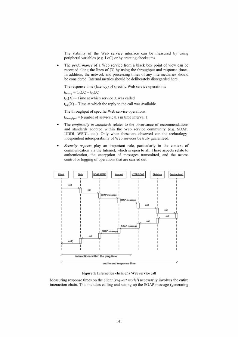
The stability of the Web service interface can be measured by using peripheral variables (e.g. LoC) or by creating checksums.
• The performance of a Web service from a black box point of view can be recorded along the lines of [3] by using the throughput and response times. In addition, the network and processing times of any intermediaries should be considered. Internal metrics should be deliberately disregarded here.
The response time (latency) of specific Web service operations: tlatency = to/p(X) – ti/p(X) ti/p(X) – Time at which service X was called to/p(X) – Time at which the reply to the call was available
The throughput of specific Web service operations: tthroughput = Number of service calls in time interval T
• The conformity to standards relates to the observance of recommendations and standards adopted within the Web service community (e.g. SOAP, UDDI, WSDL etc.). Only when these are observed can the technology-independent interoperability of Web services be truly guaranteed.
• Security aspects play an important role, particularly in the context of communication via the Internet, which is open to all. These aspects relate to authentication, the encryption of messages transmitted, and the access control or logging of operations that are carried out.
Figure 1: Interaction chain of a Web service call
Measuring response times on the client (request model) necessarily involves the entire interaction chain. This includes calling and setting up the SOAP message (generating
141
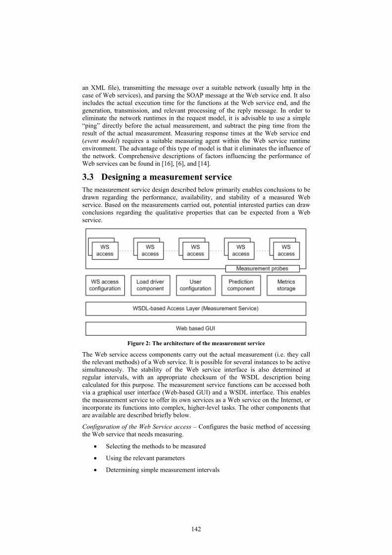
an XML file), transmitting the message over a suitable network (usually http in the case of Web services), and parsing the SOAP message at the Web service end. It also includes the actual execution time for the functions at the Web service end, and the generation, transmission, and relevant processing of the reply message. In order to eliminate the network runtimes in the request model, it is advisable to use a simple “ping” directly before the actual measurement, and subtract the ping time from the result of the actual measurement. Measuring response times at the Web service end (event model) requires a suitable measuring agent within the Web service runtime environment. The advantage of this type of model is that it eliminates the influence of the network. Comprehensive descriptions of factors influencing the performance of Web services can be found in [16], [6], and [14].
3.3 Designing a measurement service The measurement service design described below primarily enables conclusions to be drawn regarding the performance, availability, and stability of a measured Web service. Based on the measurements carried out, potential interested parties can draw conclusions regarding the qualitative properties that can be expected from a Web service.
Figure 2: The architecture of the measurement service
The Web service access components carry out the actual measurement (i.e. they call the relevant methods) of a Web service. It is possible for several instances to be active simultaneously. The stability of the Web service interface is also determined at regular intervals, with an appropriate checksum of the WSDL description being calculated for this purpose. The measurement service functions can be accessed both via a graphical user interface (Web-based GUI) and a WSDL interface. This enables the measurement service to offer its own services as a Web service on the Internet, or incorporate its functions into complex, higher-level tasks. The other components that are available are described briefly below.
Configuration of the Web Service access – Configures the basic method of accessing the Web service that needs measuring.
• Selecting the methods to be measured
• Using the relevant parameters
• Determining simple measurement intervals
142

• Dealing with error conditions.
Load driver component – Enables an appropriate load mix to be configured, so that several Web service functions can be executed virtually simultaneously.
• Defining the behavior of method calls in relation to each other
• Defining target response times
• Substituting data to be transmitted.
User configuration & access – Assigns roles and access rights for measurement service users. Read access and also the right to measure new Web services can be assigned.
• Assigning read access to all visitors of the measurement service
• Assigning read and write access to administered users.
Prediction component – Provides a calculation procedure for predicting the performance of a Web service under a given load profile.
• Configuring the anticipated load profile
• Using a solution method based on the operational analysis.
Metrics storage & export component – Stores measurements and converts them to an appropriate format for transmission (e.g. XML).
• Storing measurements in a local database
• Preparing measurements for further processing.
There are many factors that influence the performance of Web services (particularly the associated network runtimes). As mentioned above, our current plan for isolating network runtimes involves transmitting a simple PING to the server on which the Web service runs directly before the actual measurement, and subtracting this PING time tping from the overall runtime tRTT (“round trip time” of a SOAP-RPC) when measuring the Web service functions. Although measurement errors cannot be entirely eliminated in this way, we feel they can be significantly reduced. So the actual response time ta (excluding network time) for a Web service is made up as follows: ta=tRTT-tping
4 A prototype measurement service An initial prototype measurement service is currently being implemented at the software measurement laboratory of the Otto von Guericke University in Magdeburg, in collaboration with T-Systems International (Berlin Development Center). The current version allows you to measure any Web service that is available on the Internet.
143
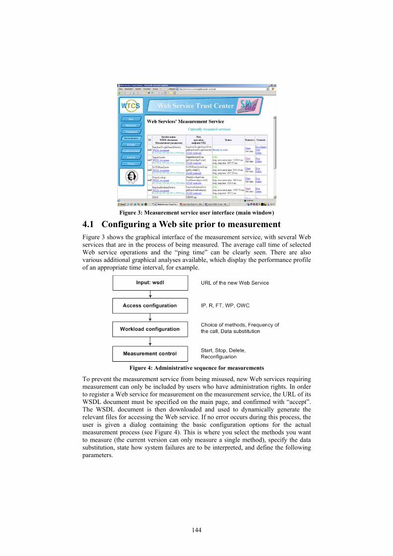
Figure 3: Measurement service user interface (main window)
4.1 Configuring a Web site prior to measurement Figure 3 shows the graphical interface of the measurement service, with several Web services that are in the process of being measured. The average call time of selected Web service operations and the “ping time” can be clearly seen. There are also various additional graphical analyses available, which display the performance profile of an appropriate time interval, for example.
Figure 4: Administrative sequence for measurements
To prevent the measurement service from being misused, new Web services requiring measurement can only be included by users who have administration rights. In order to register a Web service for measurement on the measurement service, the URL of its WSDL document must be specified on the main page, and confirmed with “accept”. The WSDL document is then downloaded and used to dynamically generate the relevant files for accessing the Web service. If no error occurs during this process, the user is given a dialog containing the basic configuration options for the actual measurement process (see Figure 4). This is where you select the methods you want to measure (the current version can only measure a single method), specify the data substitution, state how system failures are to be interpreted, and define the following parameters.
144

R - Batch length (number of repeat invocations)
In order to reduce measurement errors, it makes sense to execute the method call several times. Parameter R can be used to specify the number of successive repetitions of an operation call within a series. The result of a measurement is calculated as the average of the individual measurements within a series.
IP - Invocation period of a SOAP operation
This parameter is used to configure the call interval for the selected methods of the Web service. The time period between each series of measurements is specified in minutes.
FT - Failure tolerance
Permitted number of successive failed measurement series. A series is considered to have failed if at least one measurement (ping or operation call) in this series has failed. This parameter is useful because some Web services are occasionally temporarily unavailable.
WP - Period of checking for stability of WSDL description
Interval for checking the WSDL document for stability (potential changes), in minutes. The check involves the WSDL file being repeatedly read over the Internet, a checksum being calculated based on the Adler32 algorithm, and this checksum being compared with the previous checksum.
OWC - Be optimistic if the WSDL description changes
If the WSDL document has been changed, the parameters selected during the previous configuration or reconfiguration (i.e. service, port, and SOAP operation) may no longer be valid. The program can react to this either optimistically or pessimistically. In the former case, it will attempt to call the operation again in the next series as if nothing had happened; in the latter case, the measurement process is suspended and a reconfiguration of the Web service unit is requested.
Measurement parameters for Web services that are already being measured can only be configured if the measurements are stopped. The overview of measured Web services displays the following measurement parameters: “R=..., IP=..., WP=..., FT=..., OWC=...”.
4.2 Internal states of the measurement service Various items of status information are used to display how the measurement service is getting on with the registered Web services. These different states are necessary in order to react to changes to the Web service, and to permit the self-monitoring of the measurement service.
• Not configured – A Web service requiring measurement has either not been configured at all, or the configuration has been aborted or has failed.
• Ready to start – A Web service has been configured, but the measurement process has either not commenced, or has been suspended. The measurement will be automatically restarted following successful reconfiguration provided the “auto_start” parameter in the configuration file is set to “true”.
145
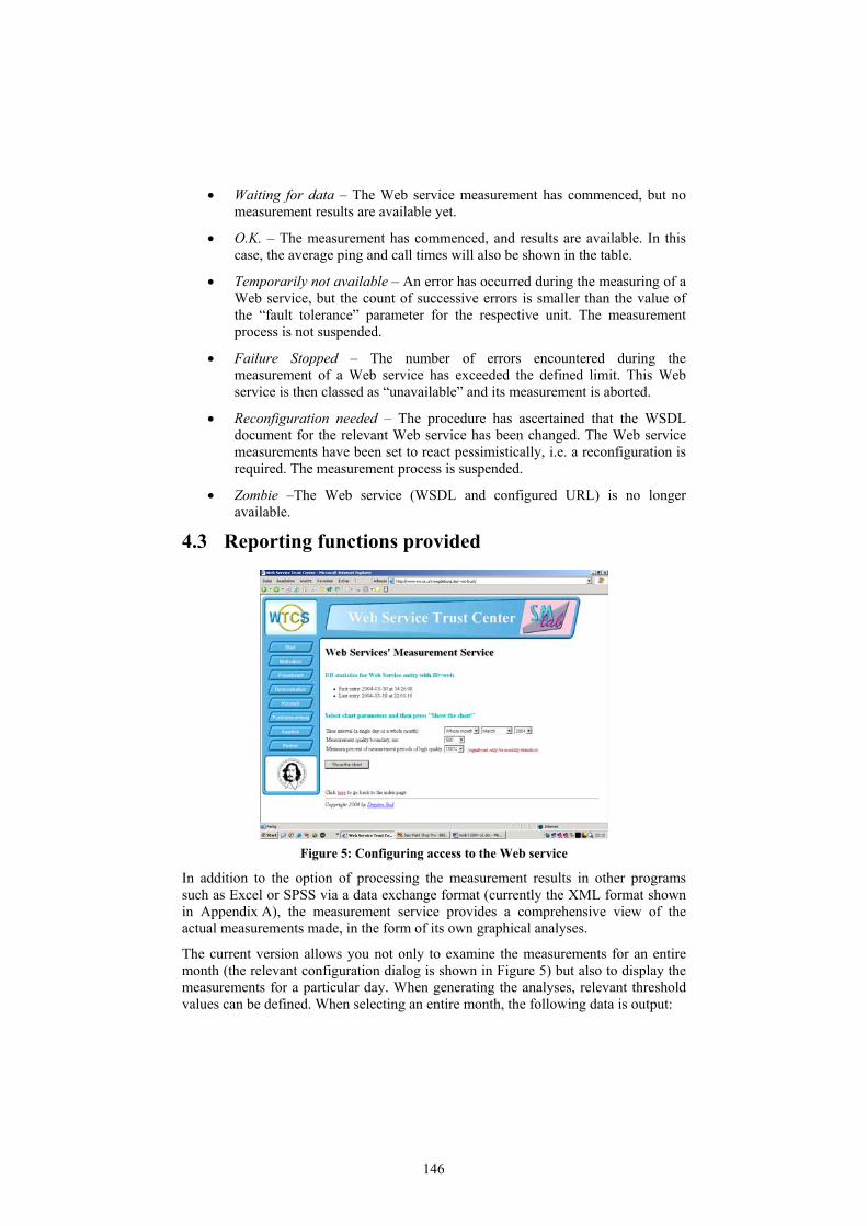
• Waiting for data – The Web service measurement has commenced, but no measurement results are available yet.
• O.K. – The measurement has commenced, and results are available. In this case, the average ping and call times will also be shown in the table.
• Temporarily not available – An error has occurred during the measuring of a Web service, but the count of successive errors is smaller than the value of the “fault tolerance” parameter for the respective unit. The measurement process is not suspended.
• Failure Stopped – The number of errors encountered during the measurement of a Web service has exceeded the defined limit. This Web service is then classed as “unavailable” and its measurement is aborted.
• Reconfiguration needed – The procedure has ascertained that the WSDL document for the relevant Web service has been changed. The Web service measurements have been set to react pessimistically, i.e. a reconfiguration is required. The measurement process is suspended.
• Zombie –The Web service (WSDL and configured URL) is no longer available.
4.3 Reporting functions provided
Figure 5: Configuring access to the Web service
In addition to the option of processing the measurement results in other programs such as Excel or SPSS via a data exchange format (currently the XML format shown in Appendix A), the measurement service provides a comprehensive view of the actual measurements made, in the form of its own graphical analyses.
The current version allows you not only to examine the measurements for an entire month (the relevant configuration dialog is shown in Figure 5) but also to display the measurements for a particular day. When generating the analyses, relevant threshold values can be defined. When selecting an entire month, the following data is output:
146

• Number of days in the selected month for which there is measurement data in the database;
• Number of days on which the required quality was achieved;
• Percentage of days on which the required quality was achieved;
• Total number of measurements carried out in the selected month;
• Number of failed measurements;
• Number of changes to the WSDL document detected in the selected month.
Figure 6 shows the measurement output for a complete day. Both the ping time and the actual call time (invocation time) of the Web service functionality are displayed. Users also receive the following information relating to the day (not shown in Figure 6):
• Number of measurements carried out on the selected day;
• Number of failed measurements on the selected day;
• Number of measurements for the day that were of the required quality;
• The relative proportion of these (%);
• Number of changes to the WSDL document detected on the selected day.
Figure 6: Results display for measurements carried out
5 Analysis of a specific Web service The Web service “XigniteQuotes” was subject to an appropriate analysis with the aid of the measurement service. This Web service provides information on share prices and indices on the US stock market. A total of 17 methods are provided for querying this information. In an initial analysis, the method GetQuickQuotes was subjected to an initial test using the measurement service. After a delay of 20 minutes, this provided the relevant share price, with information on the previous price, the percentage change, and the new price being supplied. The measurement was configured using the following values:
147

R=2; IP=120; WP=1440; FT=4, OWC=true
In line with the configuration, 2 test samples were carried out for each measurement (R=2), with the measurement itself taking place every 120 minutes (IP=120), and a check every 1440 minutes to ascertain whether the WSDL file had changed. Parameter FT was used to define the permitted number of successive errors (in this case, 4) after which the Web service is classed as being unavailable. The parameter OWC=true specifies that the service is to behave optimistically in the case of a potential change to the WSDL file, i.e. measurements will continue to be taken. This service was monitored from July 19, 2004 until the end of 2004. With reference to the days on which the relevant measurements were carried out, it was possible to validate the series of measurements and identify potential faults in the measurement service itself. This led to a fault being identified in the measurement service in the months of August and September. For the remainder of the analysis, we shall concentrate on the month of October. An overview of the results obtained in October:
• average call time (1st measurement): 1072 ms
• average call time (2nd measurement): 547 ms
• average network time (ping time): 217 ms
• measurement errors identified: 4 (i.e. 1st and 2nd measurements greater than 3 seconds)
• network errors identified (ping time > 1 sec): 1
• Checks carried out: 369 – availability 99.08%.
Basically, the series of measurements carried out established that the time for the first call is greater than that for subsequent calls. This is due to the Web service being initialized, leading to the generation of object instances during the first call. This is also highlighted in Figures 7 and 8, with this feature also being evident when other Web services were measured (not shown here).
-10000
0
10000
20000
30000
40000
50000
60000
70000
80000
1 72 143 214 285 356
Measurement 1-369
Resp
onse
tim
e in
ms
1stmeasurement2ndmeasurement
Figure 7: Response time behavior for 1st and 2nd measurement
Figure 7 shows a comparison between the 1st and 2nd measurements for the entire month of October.
148

0
2000
4000
6000
8000
10000
12000
1 70 139 208 277 346
Measurements
Resp
onst
ime
in m
s1stmeasurement2ndmeasurement
Figure 8: Adjusted measurements excluding response times > 10 secs
In order to accentuate the effect of the slower response times for the 1st measurement, we adjusted the measurement results for values greater than 10 seconds (see Figure 8).
0
100
200
300
400
Response time
Num
ber
of m
easu
rem
ents
1stmeasurements
191 74 69 35
2ndmeasurements
348 15 2 4
0.4 - 1.0 sec
1.0 - 2.0 sec
2.0 - 5.0 sec
> 5.0 sec
Figure 9: Comparison of 1st and 2nd measurements
Figure 9 shows the distribution of the results from the 1st and 2nd measurements. The difference between the 1st and 2nd measurements can be clearly seen here as well.
6 Summary and prospects The Web services currently available on the Internet vary from simple functions (simple services) such as weather or authentication services to complete business transactions such as booking all the services required in a travel portal (combined services). The more attractive the Web service functions on offer, the greater the number of potential users and therefore the load on the hardware and software resources used by the service. In a commercial environment, this gives rise to costs that should be charged to the customer accordingly. The supplier must also ensure the qualitative properties of the Web service.
149
In this context, it makes sense to use an independent measurement service, thus supporting the establishment of a wide variety of SLA-supported settlement models. The software measurement laboratory is currently working on implementing an appropriate billing component that will provide configurable business models for marketing Web services. However, it is not possible to carry out access-related settlement with the existing Web service specifications. Either the Web service itself could provide the relevant access statistics, or an appropriate broker could log the accesses. A suitable initial approach can be found in the WSLA specification (see [4]).
We are also focusing on the prediction component. The aim is to infer the future qualitative behavior of the Web service from an existing empirical base of experience. In the context of the performance properties of the Web service, a simple forecasting model is currently being implemented based on the operational analysis. However, implementing this procedure for existing Web services will not be straightforward. An extension of the interface specification to include details of the efficiency of the Web service, or alternatively the provision of an explicit test access would permit further progress in this area. In addition, the measurement service is being embedded in an appropriate Web service trust center that registers Web services available on the Internet in a directory structure and provides appropriate valued-added services, some of which build on the functionality of the measurement service we have described here.
7 References [1] Alonso, G.; Casati, F.; Kuno, H.; Machiraju, V.: Web Services – Concepts,
Architectures and Applications, Springer Berlin Heidelberg, 2004 [2] Dumke, R.; Schäfer, U.; Wille, C.; Zbrog, F.: Agent-based Web technology
evaluation for the performance engineering (only in German), in Proc. of PE2004 [3] ISO 14756: Measurement and rating of performance of computer-based software
systems. ISO/IEC JTC1/SC7 Secretariat, CANADA, 1997 [4] Keller, A.; Ludwig, H.: The WSLA Framework: Specifying and Monitoring
Service Level Agreements for web Services, IBM Research Report, May 2002 [5] Menascé, D.: Scaling the Web - QoS Issues in Web Services, IEEE Internet
Computing, vol. 6, no. 6 pp. 72–75, NOVEMBER/DECEMBER 2002 [6] Menascé, D.; Almeida, V.: Capacity Planning for Web services, Prentice Hall,
Upper Saddle River, NJ, 2002 [7] Menascé, D.; Ruan, H.; Gomaa, H.: A framewok for QoS-Aware Software
Components, in Proc. of WOSP 2004 [8] Patel, C.; Supekar, K.; Lee, Y.: A QoS Oriented Framework for Adaptive
Management of Web Service based Workflows, University of Missouri-Kansas City, 2003
[9] QoS for Web Services: Requirements and Possible Approaches, W3C Working Group Note 25 November 2003, URL: http://www.w3c.or.kr/kr-office/TR/2003/ws-qos/
[10] Sahai, A.; Machiraju, V.; Sayal, M.; Jin, L. J.; Casati, F.: Automated SLA Monitoring for Web Services, in Feridun, M.; Kropf, P. G.; Babin, G. (Eds.): Management Technologies for E-Commerce and E-Business Applications, LNCS 2506 Springer 2002
150
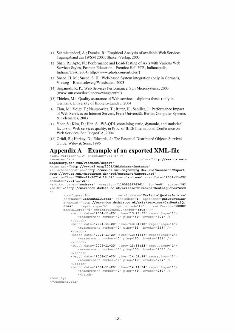
[11] Schmietendorf, A.; Dumke, R.: Empirical Analysis of available Web Services, Tagungsband zur IWSM 2003, Shaker-Verlag, 2003
[12] Shah, R.; Apte, N.: Performance and Load-Testing of Axis with Various Web Services Styles, Pearson Education - Prentice Hall PTR, Indianapolis, Indiana/USA, 2004 (http://www.phptr.com/articles/)
[13] Sneed, H. M.; Sneed, S. H.: Web-based System integration (only in German), Vieweg – Braunschweig/Wiesbaden, 2003
[14] Sriganesh, R. P.: Web Services Performance, Sun Microsystems, 2003 (www.sun.com/developers/evangcentral)
[15] Thielen, M.: Quality assurance of Web services – diploma thesis (only in German), University of Koblenz-Landau, 2004
[16] Tian, M.; Voigt, T.; Naumowicz, T.; Ritter, H.; Schiller, J.: Performance Impact of Web Services on Internet Servers, Freie Universität Berlin, Computer Systems & Telematics, 2003
[17] Yoon S.; Kim, D.; Han, S.: WS-QDL containing static, dynamic, and statistical factors of Web services quality, in Proc. of IEEE International Conference on Web Services, San Diego/CA, 2004
[18] Orfali, R.; Harkey, D.; Edwards, J.: The Essential Distributed Objects Survival Guide, Wiley & Sons, 1996
Appendix A – Example of an exported XML-file <?xml version="1.0" encoding="utf-8" ?> <wesementData xmlns="http://www.cs.uni-magdeburg.de/~rud/wesement/Export" xmlns:xsi="http://www.w3.org/2001/XMLSchema-instance" xsi:schemaLocation="http://www.cs.uni-magdeburg.de/~rud/wesement/Export http://www.cs.uni-magdeburg.de/~rud/wesement/Export.xsd" creationTime="2004-11-20T14:18:37" user="andreas" startDate="2004-11-20" endDate="2004-11-21"> <entity owner="andreas" creation="1100953476361" id="ws8" state="OK" wsdlUrl="http://wavendon.dsdata.co.uk/axis/services/CarRentalQuotes?wsdl">
<configuration serviceName="CarRentalQuotesService" portName="CarRentalQuotes" operIndex="1" operName="getCountries" endpoint="http://wavendon.dsdata.co.uk/axis/services/CarRentalQuotes" repeatings="1" operPeriod="10" wsdlPeriod="10080" maxFailures="0" optimisticWsdlChanges="true" />
<batch date="2004-11-20" time="13:29:35" repeatings="1"> <measurement number="0" ping="49" invoke="304" />
</batch> <batch date="2004-11-20" time="13:31:12" repeatings="1">
<measurement number="0" ping="53" invoke="249" /> </batch> <batch date="2004-11-20" time="13:41:17" repeatings="1">
<measurement number="0" ping="50" invoke="251" /> </batch> <batch date="2004-11-20" time="13:51:23" repeatings="1">
<measurement number="0" ping="53" invoke="253" /> </batch> <batch date="2004-11-20" time="14:01:28" repeatings="1">
<measurement number="0" ping="49" invoke="257" /> </batch> <batch date="2004-11-20" time="14:11:34" repeatings="1">
<measurement number="0" ping="49" invoke="250" /> </batch>
</entity> </wesementData>
151

152
Performance Distributions of Continuous Time Single
Server Queueing Model with Batch Renewal Arrivals:
GIG/M/1/N ∗
Wei Li, Rod Fretwell, Demetres KouvatsosPerformance Modelling and Engineering Research Group
University of Bradford, Bradford, UK, BD7 1DPemail:{w.li1, r.j.fretwell, and [email protected]}
Abstract
It has been proven that the batch renewal process (BRP) is the least biased process given the infinitesets of measures of the traffic correlation, (i.e. indices of dispersion, covariance or correlation function) inthe discrete time domain. The similar argument is expected for the continuous time BRP but not shown inhere.
The correlation induced by BRP is analysed and a queueing model fed by BRP is studied. In this context,a continuous time GIG/M/1/N queueing model is analysed having a single server, general batch renewalarrival process, exponential service time and finite buffer size N . Closed form expressions for performancedistribution, such as, queue length, blocking probability and waiting time distributions are derived. As aconsequence, these analytic tools can be used to efficiently assess the adverse effect of traffic correlationinduced by the BRP on the queue.
Keywords: batch renewal process (BRP),continuous time queueing model, performance distributions, correla-tion
1 Introduction
A persistent problem in the field of performance modelling and evaluation is to choose the most appropriatequeueing model. Unfortunately, due to the need for analytical tractability most works assume a Poisson arrivalprocess [9], which is not realistic as shown, for example in [12]. On the other hand, in actual networks, such asIP or ATM networks, it is most possible that packets arrive at the queue in batches rather than individually.
Recently, queueing models fed by batch arrival process have received significant attention [6-11]. Most of theresearch work falls in the discrete time domain, whilst batch arrival process could be also applied into continuoustime domain. The latter removes the restriction that the packets, in discrete time domain, must arrive at theend of a time slot.
BRP is a general case of batch arrival process which involves both count and interval correlations. Notethat indices of dispersion have long been known as powerful tools in the analysis of the second-order propertiesof point processes [13] [14] and computer traffic measurements [1-5].
Sriram and Whitt [1] analysed superposition of bursty correlated arrival processes in terms of indices ofdispersion for intervals (IDI). Heffes and Lucantoni [2] modelled the superposition of bursty arrival processesapproximated by a correlated Markov modulated Poisson process (MMPP) matching three features of indicesof dispersion for counts (IDC) and mean arrival rate. Gusella [3] characterized the variability of measuredpacket arrival process with indices of dispersion and discussed the merits of these indices as well as the pitfallsof their indiscriminate use. Moreover he estimated the indices of dispersion for measured LAN traffic which
∗This work is partially supported by the EU Network of Excellence (NoE) Euro-NGI.
153

was approximately modelled by 2-phase MMPP which matched on the three IDCs and the squared coefficientof variation (SCV) of the inter-arrival times.
Fowler and Leland [14] reported LAN traffic with unbounded IDC. However, it is expected that performanceof a restricted buffer system with deterministic service would not be affected by the magnitude of IDC for longintervals. Andrade and Martinez-Pascua showed that the queue length distribution and other statistics areaffected by IDC only up to a certain size of interval (determined by the buffer size) whilst the value of the IDCat infinity is of little importance.
Only a limited number of papers studying on finite-buffer queues with batch renewal process have appearedso far in the literature. In this context, the batch renewal process in a discrete time domain was introducedand applied to the analysis of queueing models by Fretwell and Kouvatsos [5-7], where the generating functionsof IDI and IDC were expressed in terms of corresponding generating functions of batch inter-arrival time andbatch size distributions. Moreover, Frey [15] analysed a finite-capacity vacation queue with batch arrivals butconsidered batch Poisson arrivals only. Niu [9] studied a vacation queue with setup and close-down times andbatch Markovian arrival processes in discrete time domain. A queueing model with batch arrivals and batch-dedicated servers was analysed by Gullu [11], which nevertheless, has an infinite number of servers and buffersizes. Finally, Takaki and Wu [10] studied queue fed by a semi-Markovian batch arrival process but with infinitewaiting rooms.
The BRP is employed in the continuous time domain and the following analysis of a GIG/M/1/N queuewith a general batch renewal arrival process GIG, as defined in Section 2. Performance distributions of queuelength, blocking probability and waiting time distributions are determined.
Section 2 introduces the continuous time batch renewal process and associated properties. Section 3 gives thetransforms of IDI and IDC of continuous time batch renewal process. The performance distributions of a singleserver queue with batch renewal arrival process and finite-capcacity are presented in Section 4. Conclusions aredrawn in Section 5.
2 Batch Renewal Processes
A batch renewal process as a traffic process allows simultaneous arrivals such that
• the number of arrivals in different batches are independent and identically distributed
• the intervals between batches are independent and identically distributed
• the batch sizes (number of arrivals in one batch) are independent of intervals between batches
In the continuous time domain, a batch renewal process has continuous inter-arrival times and discrete counts.In the discrete time domain a batch renewal process has been found to exhibit both interarrival correlationbetween individual arrivals and count correlation between successive epochs. In this paper the correspondingcorrelations are investigated in the context of a continuous time batch renewal process.
3 Correlation in Batch Renewal Process
Consider a continuous time batch renewal process in which
• the distribution of batch size is given by the probability mass function (pmf) b(n), n = 1, 2, . . ., withmean b, squared coefficient of variation (SCV) C2
b and probability generating function (pgf) B(z) =∑∞n=1 b(n)zn.
• the distribution of interval between batches is given by the probability density function (pdf) a(t), t > 0,with mean a, SCV C2
a and Laplace transform A(θ) =∫ ∞0
a(t)e−θtdt.
154

Let ν(n, t) be the probability that exactly n customers arrive during the interval of length t, n = 0, 1, . . .,t > 0. Then the transform function of ν(n, t) is defined as
N(z, θ) =∞∑
n=0
∫ ∞
t=0
ν(n, t)zne−θtdt (1)
=1θ− 1
a · θ2· (1 − A(θ))(1 − B(z))
1 − A(θ)B(z)
The IDC, It, is defined to be the variance of the number of arrivals during an interval of length t divided bythe mean number E(Nt) of arrivals in t, namely
It =V ar(Nt)E(Nt)
(2)
Let I(θ) to be the generating function of It. From the well-known connection between the indices of dispersionand correlation functions (covariances), the transform of count correlation function K(θ) can be determined by(c.f.[16]):
K(θ) = b
(C2
b +1 + A(θ)1 − A(θ)
− 2a· 1θ
)(3)
Let τ(n, t) be the probability that there are n intervals between n + 1 successive individual arrivals duringinterval of length t. Then the transform function of τ(n, t) is defined as
T (z, θ) =∞∑
n=0
∫ ∞
t=0
τ(n, t)zne−θtdt (4)
=1
1 − z− z
b · (1 − z)2· (1 − A(θ))(1 − B(z))
1 − A(θ)B(z)
The IDI, Jn, is defined to be the n times SCV of intervals X between individual arrivals.
Jn =n · V ar(X)
E(X)2(5)
Defining J(z) to be the generating function of Jn. The transform of interval correlation function L(z) canbe obtained by
L(z) = b
(C2
a +1 + B(z)1 − B(z)
− 1b· 1 + z
1 − z
)(6)
Note that K(θ) is expressed in terms of batch interarrival time distribution and L(z) in terms of batch sizedistribution.
From equations (3) and (6), A(θ) and B(z) can be expressed in terms of K(θ) and L(z), repectively, by:
1 − B(z) =2b
L(z) − b(C2a − 1) +
1 + z
1 − z
(7)
1 − A(θ) =2b
K(θ) − b(C2b − 1) + 2λ · 1
θ
(8)
It may be shown that equations (7) and (8) define A(θ) and B(z) uniquely given K(θ) and L(z) (c.f.[15]).It may be also shown that counting process ν(n, t) and timing process τ(n, t), taken together, define A(θ) andB(z) uniquely.
155

4 Censored GIG/M/1/N Queue
This section specifies the GIG/M/1/N queue and derives the performance distributions.
4.1 Model Discription and Specification
Consider a GIG/M/1/N queue with a batch renewal arrival process where customers within an arriving batchare turned away and simply lost (i.e. censored arrivals) when the number of occupied buffers reaches capacityN . The service times are assumed to be exponentionally distributed and the first customer arriving to anempty system receives service immediately and departs after serivce completion (immediate service policy). Inthe following sections, a(t) denotes the probability density function of inter-arrival time between batches, b(n)the probability mass function of batch sizes and N(0 < N < ∞) the buffer size of the queue.
4.2 Two Embedded Processes
Consider within a continuous time domain two processes embedded at points immediately before and after eachbatch arrivals. Each process may be described independently by a Markov chain but the processes are mutuallydependent.
• For the first chain (chain ‘A’), the state is the number of customers in the queue after allowing for anydeparture at that instant but discounting the new arrivals at that instant. Let PA
N (n) be the steady stateprobability that the state be n = 0, 1, · · · , N − 1 (where N is the capacity of the system)
• For the second chain (chain ‘D’), the state is the number of customers in the queue after allowing for anydeparture at that instant but including the new arrivals. Let PD
N (n) be the steady state probability thatstate be n = 1, 2, · · · , N
• Let PN (n) be the steady state probability that there are n = 0, 1, · · · , N customers in the system (includ-ing queueing and receiving service) at any time
To see the relation between the two Markov chains, first consider the state of each chain at an arrival instant.Chain ‘D’ may be in state n = 1, 2, · · · , N − 1 when chain ‘A’ is in state k = 0, 1, · · · , n − 1 and there are n − karrivals in the batch. Alternatively, chain ‘D’ may be in state N when chain ‘A’ is in state k = 0, 1, · · · , N − 1and there are at least N − k arrivals in the batch, therefore
PDN (n) =
⎧⎪⎪⎪⎪⎨⎪⎪⎪⎪⎩
n−1∑k=0
PAN (k)b(n − k) n=1,2,· · ·,N-1
N−1∑k=0
PAN (k)
∞∑r=N−k
b(r) n=N(9)
Now consider the states of each chain at successive arrival instants. At the later instant, the chain ‘A’ maybe in state n = 1, 2, · · · , N − 1 when the chain ‘D’ may be in state k = n + 1, · · · , N at earlier arrival instantand there are k − n departures in the interval between two arrivals of batches. Since the service times areexponentially distributed, the probability that k − n customers depart during interval of length t is given by
∫ ∞
0
eµt · (ut)k−n
(k − n)!dt (10)
156

The realtionship between PAN and PD
N at two successive arrival instants
PAN (n) =
⎧⎪⎪⎪⎪⎨⎪⎪⎪⎪⎩
N−n∑k=0
PDN (n + k)
∫ ∞
0
e−µt · (µt)k
k!· a(t)dt n = 1, 2, · · · , N
N∑k=0
PDN (k)
∫ ∞
0
∫ t
0
e−µs · (µs)k
k!ds · a(t)dt n = 0
(11)
4.3 Queue Length Distribution
If immediately after the arrival of a batch, there are n+k = 1, 2, · · · , N customers in the system and the intervalbetween that and the next batch be the length of t, then
PN (n) =
⎧⎪⎪⎪⎪⎨⎪⎪⎪⎪⎩
N−n∑k=0
PDN (n + k)
∫ ∞
0
∫ t
0
e−µs · (µs)k
k!· 1a· ds · a(t)dt n = 1, 2, · · · , N
N∑k=1
PDN (k)
∫ ∞
0
∫ t
0
e−µs · (µs)k
k!· 1a· (t − s) · ds · a(t)dt n = 0
(12)
4.4 Blocking probability
If an arriving batch of size N − k + r finds k customers in the finite buffer system, then only the first N − kcustomers of the arriving batch enter the system and r customers will be blocked and lost.
The probability that the arriving batch finds k customers is PAN (k), the probability that the batch be of size
N − k + r is (N − k + r) · 1b · b(N − k + r) and the probability of a customer being in one of the r positions,
given tha batch being of size N − k + r, isr
N − k + r. Therefore, the blocking probability ΠB
N is given by
ΠBN =
N−1∑k=0
PAN (k)
∞∑r=1
r
bb(N − k + r) (13)
4.5 Waiting time distribution
The waiting time of a customer is given by the interval from the instant at which it arrives in the queue to thatit is receiving service.
If the new arrival batch finds k customers in the system, then the waiting time be the service time of kcustomers plus the service time of i − 1 customers before the tagged customer given it is in the ith position inthe batch.
WN (t) =
∑N−1k=0
∑∞r=i
∑N−kr=1 PA
N (k)b(r)∫ ∞0
(µt)k+i−2·µ(k+i−2)! e−µtdt
b(1 − ΠBN )
(14)
5 Conclusions
A continuous time GIG/M/1/N queue with single server, general batch renewal arrivals process, exponentiallydistributed service time and finite capacity N is analysed. Closed form expressions for basic performancedistributiions, such as queue length, waiting time and blocking probability distributions are derived. As aconsequence, these analytic tools can be used to efficiently assess the adverse effect of traffic correlation inducedby the BRP on the queue.
Numerical results on the effects of correlation on the behaviour of queueing system will be given in a sequelpaper.
157
References
[1] Kotikalapudi Sriram, Ward Whitt, Characterizing Superposition Arrival Porcesses in Packet Multiplexersfor Voice and Data, IEEE Journal on Selected Areas in Communication, Vol. SAC-4, No. 6, pp. 833-846,September 1986
[2] Harry Heffes, David M. Lucantoni, A Markov Modulated Characterization of Packetized Voice and DataTraffic and Related Statistical Multiplexer Performance, IEEE Journal on Selected Areas in Communication,Vol. SAC-4, No. 6, pp. 856-868, September 1986
[3] Riccardo Gusella, Characterizing the Variability of Arrival Processes with Indexes of Dispersion, IEEEJournal on Selected Areas in Communication,Vol. 9, No. 2, pp. 203-211, February 1991
[4] Leonard Kleinrock, Queueing Systems Volume1: Theory,A Wiley-Interscience Publication, John Wiley andSons, Canada, 1975.
[5] Demetres Kouvatsos, Rod Fretwell, Discrete Time Batch Renewal Processes with Application to ATM Per-formance, Proceeding of the 10th UK Performance Engineering Workshop, Hilston, J.Etal(eds.). EdinburghUniversity Press, pp. 187-192, Sep.1994
[6] Demetres Kouvatsos, Rod Fretwell, Closed Form Performance Distribution of a Discrete Time GIG/D/1/NQueue with Correlated Traffic, In Data Communications and their Performance, Fdida S. and Onvural.(eds.),Chapman and Hall, pp. 141-163, 1995
[7] R.J.Fretwell, An Investigation into traffic correlation in high speed communication networks by means ofdiscrete time models, Ph.D thesis, 2002
[8] Sebastia Galmes, Ramon Ruigjaner, Correlation analysis of a discrete-time flexible arrival process, ComputerNetworks, Vol. 41 (2002), pp. 795-814
[9] ZhiSheng Niu, Tao Shu, Yoshitaka Takahashi, A vacation queue with setup and close-down times and batchMarkovian arrival processes, Performance Evaluation, Vol. 54 (2003), pp 225-248
[10] Hideaki Takagi, De-An Wu, Multiserver queue with semi-Markovian batch arrivals, Computer Communi-cations, Vol. 27 (2004), pp 549-556
[11] Refik Gullu, Analysis of an M/G/∞ queue with batch arrivals and batch-dedicated servers, OperationsResearch Letters, Vol. 32 (2004), pp 431-438
[12] Vern Paxson, Sally Floyd, Wide-Area Traffic: The Failure of Poisson Modeling, ATM/IEEE Transactionson Networking, 3 (3), pp. 226-244, June 1995
[13] D.D.Brillinger, Comparative aspects of the study of ordinary time series and of point processes, in Devel-opment in Statistics, P.R.Krishnaiah, Ed. New York: Academic, 1978, Vol.1, pp33-133
[14] D.R.Cox and P.A.W.Lewis, The Statistical Analysis of Series of Events. London: Chapman and Hull, 1966.
[15] A.Frey, Y.Takahashi, An M [x]/GI/1/N queue with close-down and vacation time,J.Appl.Math.Stochast.Anal.12 (1999) 63-83
[16] W.Li, R.Fretwell, D.D.Kouvatsos, Continuous Time Batch Renewal Processes and the Application to Anal-ysis of Queueing Models, Research Report, May 2005
158

Abstract: IEEE 802.11 Medium Access Control (MAC) uses The Binary Exponential Backoff (BEB). BEB uses a uniform random distribution to choose the backoff value that often leads to reducing the effect of window size increment. This paper introduces a modified logarithmic backoff algorithm that uses logarithmic increment instead of exponential extension of window size to eliminate the degrading effect of random number distribution. Results from simulation experiments reveal that the new algorithm achieves higher throughput when in a mobile ad hoc environment.
Keywords: IEEE 802.11, Ad Hoc networks, Medium access control, Backoff algorithm.
1. Introduction
Mobile Ad Hoc Networks (MANETs) are getting more and more attention. The reason for this is that unlike wired networks, MANETs are easily deployed, and need no infrastructure [1]. Such networks can be useful in disaster recovery where there is not enough time or resources to configure a wired network. Ad hoc networks are also used in military operations where the units are moving around the battlefield in a random way and a central unit cannot be used for synchronization [1]. In MANETs, a central station is not needed in order to control the different types of operations taking place allover the network. A node participating in an ad hoc network must have the ability to act as a client, a server, and a router [1]. Nodes should also have the ability to connect to the network and to automatically configure to start transmitting data over the network. This is the reason why ad hoc protocols in general are functioning in a distributed manner. The distributed Coordination Function (DCF) is used for synchronous, contention-based, distributed access to the channel [3]. MANETs use a shared medium to transfer data between its nodes. The wireless medium used by MANETs has a number of problems related to it. Bandwidth sharing, signal fading, noise, interference, etc…. with such a shared medium, an efficient and effective medium access control (MAC) is essential to share the scarce bandwidth resource [12] [1]. As a part of an efficient medium access control protocol, a backoff algorithm is used to avoid collisions when more than one node try to access the channel. Only one of the nodes is granted access to the channel, while other contending nodes are suspended into a backoff state for some period (BO) [9]. Many backoff algorithms have been developed in the literature [4, 9]. One example is the Multiplicative Increase Linear Decrease (MILD) algorithm [4]. This algorithm improves the total throughput of the network, but the cost is that MILD needs a partial knowledge of the number of nodes over the network, which is a high cost knowledge.
A New Backoff Algorithm for MAC Protocol in MANETs
Saher S. Manaseer Mohamed Ould-Khaoua
Department of Computing Science University of Glasgow
Glasgow G12 8RZ {Saher, Mohamed}@dcs.gla.ac.uk
159

In a normal LAN, the total number of nodes on the network is easily obtained. However, as nodes in MANETs are mobile, knowing the number of nodes may incur a high cost, since this knowledge needs to be updated. One approach to update and keep the knowledge coherent is by exchanging “hello” packets between neighboring nodes. The “hello” packets sending process is a broadcast over the network. The broadcast generates extra traffic load over the network, consumes a part of the network resources, causes a longer delay, more control processing, and even gives more work to the backoff algorithm itself. Other backoff algorithms have tried to find a fixed optimum backoff value to use. However, the distribution functioning was not complete [8]. In the IEEE 802.11 standard MAC protocol, the Binary Exponential Backoff (BEB) is used. This algorithm functions in the following way [2]. When a node over the network has a packet to send, it first senses the channel using a carrier sensing technique. If the channel is found to be idle and not being used by any other node, the node is granted access to start transmitting. Otherwise, the node waits for an inter-frame space and the backoff mechanism is invoked. A random backoff time will be chosen in the range [0,CW-1]. A uniform random distribution is used here, where CW is the current contention window size. The following equation is used to calculate the backoff time (BO): Backoff time (BO) = (Rand () MOD CW) X aSlotTime (1) The backoff procedure is preformed then, by putting the node on a waiting period of length BO. Using carrier sense mechanism, the activity of the medium is sensed at every time slot. If the medium is found to be idle then the backoff period is decremented by one time slot. Backoff time (BO) new = (BO) old - aSlotTime (2) If the medium is determined to be busy during backoff, then the backoff timer is suspended. This means that backoff period is counted in terms of the idle time slots. Whenever the medium is idle for longer than an inter-frame space, backoff is resumed. When backoff is finished with a BO value of zero, a transfer should take place. If the node succeeds to send a packet and receive an acknowledgment, the CW for this node is reset to the minimum, which is equal to 31 in the case of BEB. If the transfer fails, the node starts another backoff period. In the next backoff period, the contention window size is exponentially increased with a maximum of 1023 [5]. BEB has a number of disadvantages. One major disadvantage is the problem of fairness [7]. BEB tends to prefer last contention winner and new contending nodes to other nodes when allocating channel access. Backoff time is decided by choosing a random backoff value from a contention window (CW) that has a smaller size for new contending nodes and contention winners. This behavior causes what is known as “Channel capture effect” in the network [10]. Another problem of BEB is related stability. BEB has been designed to be stable for large number of nodes. Studies showed that it is not [9]. The rest of this paper is organised as follows. Section 2 describes the new modified logarithmic backoff algorithm. Section 3 describes simulation environment and discusses the results and there behavior compared to IEEE 802.11 BEB algorithm.
160

Finally, Section 4 concludes the paper.
2. The modified backoff algorithm
BEB algorithm uses the following equation to increase the contention window size Backoff time (BO) = (Rand () MOD CW) X aSlotTime The new algorithm used the Logarithm of the current backoff time as the increment factor to calculate the next backoff. The following formula is used: (BO) new = (log (BO) old) X (BO) old X aSlotTime (3) This formula provides different outcome for the backoff times. The behavior of the two formulas can be seen in Figure1 and 2. The further we go with backoff; the closer will become the new values to the old values generated by the modified algorithm.
Fig. 1: CW increases in BEB.
Fig. 2: CW increases in logarithmic algorithm Figure 3 explains the modified algorithm.
161

Figure 3 The modified backoff algorithm. The main idea behind choosing such an equation for calculating backoff time is that instead of going on a back off period for X time slots, the node goes into two consecutive backoff periods say i1 and i2, where i1 + i2 ≈ X when the node is backing of for a consecutive number of times. This allows the node a chance to access the channel and transmit in a way like if backoff is stopped in the middle of the backoff period X. Reducing the channel capture effect [7] is another perspective of the new algorithm. In BEB, when a node loses in contention for channel access, there is a good chance that the next backoff timer will be double as the current value, this assigns the node larger probability to lose in the next contention against new arrivals and contention winners [10]. When using the logarithmic algorithm, the difference between the backoff periods is smaller, and so the chance of losing is not increased by the logarithmic algorithm. The cost in of using the modified algorithm is one extra invocation of the backoff handler to restart the timer. The modified algorithm also has stopped using the uniform random distribution. Which, as shown in the results in Section 4, hides the effect of the increase behavior of the CW, the thing causing research results to be masked by a side factor.
3. Simulation Results and analysis
Simulation has been performed using nine topologies with different number of nodes in each topology. The traffic over the network has been generated as Constant Bit Rate (CBR) traffic, maximum speed is 10.0 m/s, and the pause time is 10 s. Queue length is 50 packets.
Figure 4 displays the result of running the modified algorithm against the standard IEEE 802.11 binary exponential backoff algorithm. The figure shows that the throughput is higher for the modified algorithm. A network with larger number of nodes has a better throughput than the case of small number of nodes. The reason of this is, for larger number of nodes, contention is much higher and so, it is more probable for a node to backoff for more consecutive periods, this leads a more significant effect of the behavior of logarithmic algorithm and backoff values start to be closer.
162
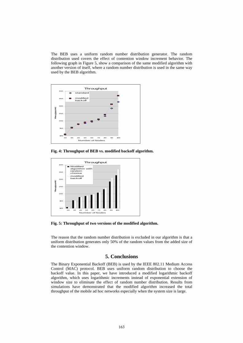
The BEB uses a uniform random number distribution generator. The random distribution used covers the effect of contention window increment behavior. The following graph in Figure 5, show a comparison of the same modified algorithm with another version of itself, where a random number distribution is used in the same way used by the BEB algorithm.
Throughput
100
150
200
250
300
350
400
20 30 40 50 60 70 80 90 100
Number of Nodes
Throug
hput KB
standard
modifiedbackoff
Fig. 4: Throughput of BEB vs. modified backoff algorithm.
Throughput
100
150
200
250
300
350
400
20 30 40 50 60 70 80 90 100
Number of Nodes
Throug
hput KB
Modifiedalgorithm withrandomchoosemodifiedbackoff
Fig. 5: Throughput of two versions of the modified algorithm. The reason that the random number distribution is excluded in our algorithm is that a uniform distribution generates only 50% of the random values from the added size of the contention window.
5. Conclusions The Binary Exponential Backoff (BEB) is used by the IEEE 802.11 Medium Access Control (MAC) protocol. BEB uses uniform random distribution to choose the backoff value. In this paper, we have introduced a modified logarithmic backoff algorithm, which uses logarithmic increments instead of exponential extension of window size to eliminate the effect of random number distribution. Results from simulations have demonstrated that the modified algorithm increased the total throughput of the mobile ad hoc networks especially when the system size is large.
163

References [1] Z.Fang, et al., “Performance evaluation of a fair backoff algorithm for IEEE
802.11 DFWMAC.” International Symposium on Mobile Ad Hoc Networking & Computing
[2] S. Xu, And T. Saadawi, “Does the IEEE 802.11 MACprotocol work well in multihop wireless ad hoc networks?” IEEE Communications Magazine, pp 130 – 137, 2001.
[3] L.Bononi, et al., "Design and Performance Evaluation of a Distributed Contention Control (DCC) Mechanism for IEEE 802.11 Wireless Local Area Networks", Journal of Parallel and Distributed Computing (JPDC), Vol. 60, N.4, April 2000, pp. 407-430.
[4] K. Sakakibara, et al., "Backoff Algorithm with Release Stages for Slotted ALOHA Systems." ECTI Transactions On Electrical Eng., Electronics, And Communications vol.3, no.1 pp 59-70 ,2005.
[5] H. Zhai and Y. Fang,”Performance of Wireless LANs Based on IEEE 802.11 protocols.” 14th IEEE International Symposium on Personal, Indoor and Mobile Radio Communication Proceedings, pp 2586-2590, 2003.
[6] K. Fall and K. Varadhaa. editors. “NS notes and Documentation.” The V l N l Project UC Berkeley. LBL. USC/ISI. and Xeros PARC. 2002
[7] B. ENSAOU, et al.,” Fair Media Access in 802.11 based Wireless Ad-Hoc Networks.” In IEEE/ACM MobiHOC (Boston, MA., August 2000).
[8] L. Bao and J. J. Garcia-Luna-Aceces, “A New Approach to Channel Access Scheduling for Ad Hoc Networks,” in ACM MOBICOM, pp. 210–221, 2001.
[9] J. Goodman, et al., “Stability of Binary Exponential Backoff”, app. In the Proc. of the 17-th Annual ACM Symp. Theory of Comp., Providence, May 1985.
[10] J. Hastad , et al., “Analysis of Backoff Protocols for Multiple Access Channels”, Siam J. Computing vol. 25, No. 4, 8/1996, pp. 740-
[11] C. Sauer, E. MacNair, "Simulation of Computer Communication Systems", Prentice-Hall, INC., 1983.
[12] F. Cali', et al.., “IEEE 802.11 Wireless LAN: Capacity Analysis and Protocol Enhancement”, Proc. INFOCOM'98, San Francisco, CA, March 29 - April 2, 1998, pp. 142-149.
164
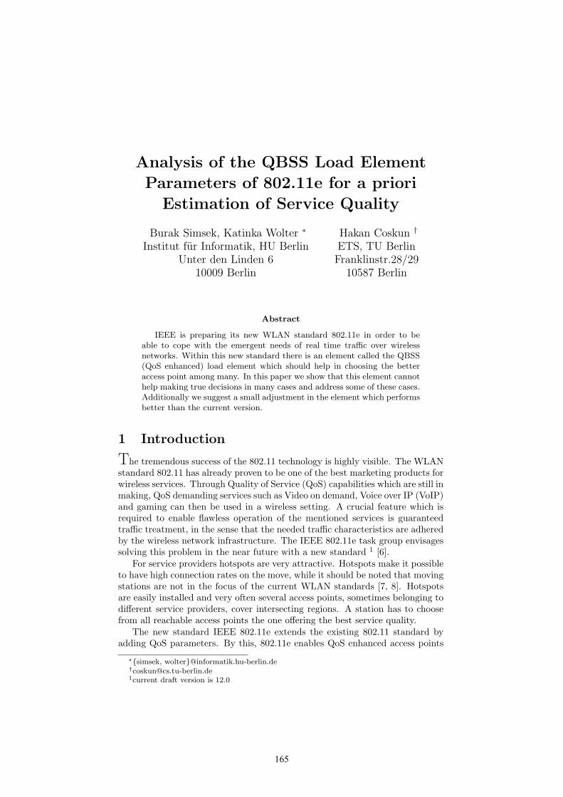
Analysis of the QBSS Load Element
Parameters of 802.11e for a priori
Estimation of Service Quality
Burak Simsek, Katinka Wolter ∗
Institut fur Informatik, HU BerlinUnter den Linden 6
10009 Berlin
Hakan Coskun †
ETS, TU BerlinFranklinstr.28/29
10587 Berlin
Abstract
IEEE is preparing its new WLAN standard 802.11e in order to beable to cope with the emergent needs of real time traffic over wirelessnetworks. Within this new standard there is an element called the QBSS(QoS enhanced) load element which should help in choosing the betteraccess point among many. In this paper we show that this element cannothelp making true decisions in many cases and address some of these cases.Additionally we suggest a small adjustment in the element which performsbetter than the current version.
1 Introduction
The tremendous success of the 802.11 technology is highly visible. The WLANstandard 802.11 has already proven to be one of the best marketing products forwireless services. Through Quality of Service (QoS) capabilities which are still inmaking, QoS demanding services such as Video on demand, Voice over IP (VoIP)and gaming can then be used in a wireless setting. A crucial feature which isrequired to enable flawless operation of the mentioned services is guaranteedtraffic treatment, in the sense that the needed traffic characteristics are adheredby the wireless network infrastructure. The IEEE 802.11e task group envisagessolving this problem in the near future with a new standard 1 [6].
For service providers hotspots are very attractive. Hotspots make it possibleto have high connection rates on the move, while it should be noted that movingstations are not in the focus of the current WLAN standards [7, 8]. Hotspotsare easily installed and very often several access points, sometimes belonging todifferent service providers, cover intersecting regions. A station has to choosefrom all reachable access points the one offering the best service quality.
The new standard IEEE 802.11e extends the existing 802.11 standard byadding QoS parameters. By this, 802.11e enables QoS enhanced access points
∗{simsek, wolter}@informatik.hu-berlin.de†[email protected] draft version is 12.0
165
(QAP) to cope with real-time traffic that is delay-sensitive, jitter-sensitive,error-prone etc. such as voice and video streams (see [1] for a detailed overview).In consequence, the whole new 802.11 series is supposed to operate on accesspoints and wireless stations with QoS enhancement (QAP and QSTAs) andwithout it (AP and STAs). The issue of QoS is addressed in the new standardIEEE 802.11e by introducing a new element called the QBSS (QoS enhancedbasic service set) load element, which is part of the beacon frames generatedby QoS enhanced access points (QAP) and contains information on the currenttraffic situation. It includes three parameters: station count, channel utilizationand available admission capacity. The station count is the total number of sta-tions currently associated with the access point. The channel utilization rate isthe normalized value of the total channel utilization which gives the percentageof the time the channel is sensed to be busy using either the physical or virtualcarrier sense mechanism of the access point. The available admission capacitygives the amount of time that can be used by explicit admission control. Thesethree parameters can be used on one hand by a QoS enhanced access point todecide whether to accept an admission control request. On the other hand theQBSS load element parameters can also be used by a wireless station to decidewhich of the available access points to choose.
Research in the area of QoS in 802.11 networks concentrates mainly on theevaluation of the performance of the 802.11e drafts and related improvementproposals [3, 4, 5]. In this paper we assume that QoS handling is given andworks as expected, the main question we strive to answer is: how should a QoSenhanced station (QSTA) decide which QoS enhanced access point to use, whenmultiple QAPs are present in its environment. Does the extension proposed inthe standard 802.11e provide sufficient information to select the appropriateaccess point?
We evaluate the significance of the three parameters of the QBSS load el-ement in a simulation study using the ns-2 network2 simulator [2], where wedetermine the coefficient of correlation with some QoS metric. Different QoSmetrics are used depending on the type of traffic (voice, video, etc) under con-sideration.
It turned out that none of the three QoS parameters of the QBSS loadelement shows a significant correlation with any of the QoS metrics for differenttypes of traffic. We conclude that the parameters of the QBSS load elementare neither sufficient nor suitable for describing the expected QoS. Instead wefound the number of already present connections of the regarded type (if we lookat video traffic that is the number of already connected video transmissions)correlates strongly with the respective QoS metric. Therefore we propose toenhance the QoS description of the QBSS load element by another field holdingthe number of existing connections.
The rest of the paper is structured as follows: After a summary of thecurrent status of the 802.11e MAC protocol and its functioning in Section 2, wepresent different scenarios that were simulated with the ns-2 network simulatorin Section 3. Section 4 discusses the simulation results in detail. Based on thegained results, we suggest an enhancement in the QBSS load element to achieveimprovements in finding the best suited QAP depending on the required QoSin Section 5. Finally, Section 6 concludes this paper.
2Several implementations of 802.11e mechanisms are already available
166

2 The Basics of the IEEE 802.11e Standard
There are two main functional blocks defined in 802.11e. These are the channelaccess functions and the traffic specification (TSPEC) management. We willin this section describe the channel access function which is a key part of thesimulation study. The main idea behind the development of the IEEE 802.11eQoS facility is the lack of sufficient QoS management over WLAN. To solvethis problem, the IEEE 802.11e task group introduced an obligatory functionfor the MAC layer called hybrid coordination function (HCF) composed of acombination of two sub functions, EDCA (enhanced distributed channel access)for prioritized channel access (similar to DiffServ) and HCCA (HCF controlledchannel access) for parameterized channel access (similar to IntServ). The HCFsplits the time frame into a contention and a contention-free period assigningit to EDCA or HCCA respectively. Different applications having different QoSrequirements are differentiated and handled correspondingly using one or bothof these functions.
In the draft, there exists a new central control mechanism of HCF which iscalled the hybrid coordinator (HC). The hybrid coordinator, which is collocatedat the QoS enhanced access points, is responsible for the management of the useof EDCA and HCCA in a cooperative manner. Basically the hybrid coordinatormakes the decision about when and how to use EDCA and HCCA, it assignstransmission opportunities (TXOP) to the stations defining the time intervalin which they are allowed to send their MPDUs (MAC Protocol Data Unit).TXOPs can be given by using one of these two functions with respect to theneeds of the stations. The HC can start a contention free period during thecontention period by sending a CFPoll (contention free poll). A possible com-bination of contention periods and contention free periods is illustrated withinthe standard draft as given in Figure 1 where a CAP is the controlled accessphase of the hybrid coordinator. As can be observed from this figure, there is noobservable regularity of the occurrences of controlled access phases. After send-ing a beacon period, hybrid coordinator starts contention free period. Followingthe end of the contention free period, contention period is started. In the sec-ond beacon period one can see that additional contention free period is startedin between two contention periods for a short period of time. A summary ofboth functions/periods and how HCF uses them is given in the following twosubsections.
DTIM
B e a c o n
B e a c o n
B e a c o n
B e a c o n
DTIM DTIM
CFP CP CFP CP
CFP Repetition Interval
EDCA TXOP s and access by legacy STAs using DCF
CAP DTIM: Delivery Traffic Information Map
Figure 1: CAP/CFP/CP periods
In the following two subsections, we try to make it clear which functional-
167

ities of EDCA and HCCA affect their behavioural prediction. This will helpunderstanding the correlation analysis of the third section.
2.1 Enhanced Distributed Channel Access (EDCA)
The enhanced distributed channel access function is defined to offer prioritizedchannel access. Traffic streams using this function are assigned user prioritiesat layers higher than the MAC layer. The assignment of user priorities is leftto the service providers offering a high flexibility for network management. Atthe MAC layer, user priorities are grouped into 4 access categories. The accessto the channel during the use of the EDCA function is also called a contentionperiod because all access categories compete with each other to win the socalled EDCA transmission opportunities. Stations receiving EDCA TXOPsare allowed to send their packets to the access point. Each access categoryhas a backoff timer that is used for the contention process and is measured inslotTimes. There is a different maximum length of the transmission opportunityassigned to each access category. Different TXOPs makes sure that channel isnot occupied with long frames of low priority packets. The maximum timelength an access category can use for sending one frame is restricted with theTXOPs.
Consequently, there are four main parameters enabling the traffic differenti-ation by the use of EDCA. These are CWmin[AC] and CWmax[AC] (minimumand maximum contention window lengths for each access category), AIFS[AC](arbitration inter frame space) and TXOPLimit[AC] (maximum duration anaccess category can use to send a frame). The values of these parameters areadvertised at the beginning of each beacon period by the access point withinthe EDCA parameter set element. This element includes all EDCA related pa-rameter values needed for the proper operation of the QoS facility during thecontention period. Access points can tune the values of these parameters duringrun time with respect to channel load situation and networking policies. Thispoint is open for further research and will be product specific on each accesspoint.
The contention procedure is very well defined for EDCA, making simplereasoning possible such as if there is more traffic on the channel, there willbe more collisions during contention. Additionally there will be more sourcesoccupying the channel if there is more traffic. These two problems increase theloss and delay rates directly. Although some exceptions exist, which will bediscussed in the third section, the loss, delay and jitter rates of traffic streamsare mostly directly proportional to the load element parameters.
2.2 HCF Controlled Channel Access (HCCA)
In case a traffic stream has some constraints which cannot be dealt with the useof EDCA, the owner of this stream can tell the access point that this specific traf-fic stream needs to be polled in the schedule of HCCA. The hybrid coordinationfunction uses HCCA in order to make sure that strict QoS requirements such asdelay and loss rates of real time traffic streams are satisfied. During transmis-sions, the hybrid coordinator has a higher medium access priority compared tonon access point stations by waiting only one point coordination function interframe space (PIFS) period, which is smaller than AIFS[AC] (see above). Thus,
168
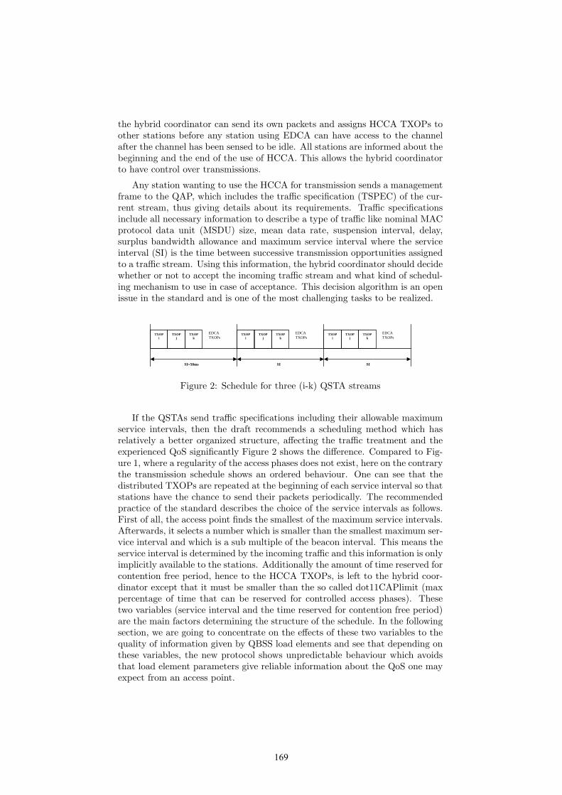
the hybrid coordinator can send its own packets and assigns HCCA TXOPs toother stations before any station using EDCA can have access to the channelafter the channel has been sensed to be idle. All stations are informed about thebeginning and the end of the use of HCCA. This allows the hybrid coordinatorto have control over transmissions.
Any station wanting to use the HCCA for transmission sends a managementframe to the QAP, which includes the traffic specification (TSPEC) of the cur-rent stream, thus giving details about its requirements. Traffic specificationsinclude all necessary information to describe a type of traffic like nominal MACprotocol data unit (MSDU) size, mean data rate, suspension interval, delay,surplus bandwidth allowance and maximum service interval where the serviceinterval (SI) is the time between successive transmission opportunities assignedto a traffic stream. Using this information, the hybrid coordinator should decidewhether or not to accept the incoming traffic stream and what kind of schedul-ing mechanism to use in case of acceptance. This decision algorithm is an openissue in the standard and is one of the most challenging tasks to be realized.
TXOP i
TXOP j
TXOP k
TXOP i
TXOP j
TXOP k
TXOP i
TXOP j
TXOP k
SI SI=50ms
EDCA TXOPs
EDCA TXOPs
EDCA TXOPs
SI
Figure 2: Schedule for three (i-k) QSTA streams
If the QSTAs send traffic specifications including their allowable maximumservice intervals, then the draft recommends a scheduling method which hasrelatively a better organized structure, affecting the traffic treatment and theexperienced QoS significantly Figure 2 shows the difference. Compared to Fig-ure 1, where a regularity of the access phases does not exist, here on the contrarythe transmission schedule shows an ordered behaviour. One can see that thedistributed TXOPs are repeated at the beginning of each service interval so thatstations have the chance to send their packets periodically. The recommendedpractice of the standard describes the choice of the service intervals as follows.First of all, the access point finds the smallest of the maximum service intervals.Afterwards, it selects a number which is smaller than the smallest maximum ser-vice interval and which is a sub multiple of the beacon interval. This means theservice interval is determined by the incoming traffic and this information is onlyimplicitly available to the stations. Additionally the amount of time reserved forcontention free period, hence to the HCCA TXOPs, is left to the hybrid coor-dinator except that it must be smaller than the so called dot11CAPlimit (maxpercentage of time that can be reserved for controlled access phases). Thesetwo variables (service interval and the time reserved for contention free period)are the main factors determining the structure of the schedule. In the followingsection, we are going to concentrate on the effects of these two variables to thequality of information given by QBSS load elements and see that depending onthese variables, the new protocol shows unpredictable behaviour which avoidsthat load element parameters give reliable information about the QoS one mayexpect from an access point.
169

3 Simulations
In order to show the information given by the QBSS load element, we runsimulations with different traffic and parameter combinations. We concentratedon the effects of the percentage of time reserved for HCF controlled channelaccess and the service interval length chosen by the access point under mixedtraffic load.
The aim of this paper is to find parameters that are indicative for QoSof each traffic type (like voice, or video traffic) in an environment exposed tomixed traffic as described below. For this purpose we measure the amount ofuseful information in the QBSS load element through its correlation with ourQoS metric of interest. The considered QoS metric depends on which type oftraffic from the traffic mixture is of interest. We expect that channel utilizationand number of connected stations show positive correlation with all QoS metricswhile the available admission capacity correlates negatively with all QoS metrics.Note that alternating sign of the correlation across the system parameters aswell as a high variability indicates low reliable expressive power of the QBSSload element.
The results of the following subsections show that, the information capturedby the QBSS load element is seemly inconsistent. Therefore we included anextra parameter in the correlation study that is the number of traffic streams ofthe different types of traffic. Traffic is divided up into different priority classesand some of the different types of traffic are associated with different priorityclasses, we therefore will discuss the priority classes rather than the traffic types.We show that this extra parameter is in many cases highly correlated withthe QoS metric and therefore we propose to include the number of stationsguaranteed the different priority levels as an additional parameter in the QBSSload element. Especially for voice and video traffic streams QoS evaluation canbe substantially improved.
3.1 Simulation Environment
We consider as infrastructure a QoS enabled basic service set (QBSS) composedof a QoS enabled access point (QAP) and a number of stations (QSTAs) associ-ated with the QAP. A slightly modified version of Qiang Ni’s ns2 implementationof EDCF/HCF is used to perform simulation runs based on this infrastructure[9].
Although 802.11e defines many parameters, we focused on the service inter-val (SI) and the relative amount of time reserved for HCCA as system specificvariables. Together with the considered traffic types, we input a total of threevariables. We define 7 different traffic types similar to the work in [3, 5, 12] asfollows.
1. Bidirectional constant bit rate (CBR) voice traffic using UDP with a packet sizeof 160 bytes and packet interval 20ms (8 Kbytes/s) corresponding to the VoIPcodec G.711. (1st access category)
2. CBR video traffic using UDP with a packet size 1280 bytes and packet intervalof 10ms (128 Kbytes/s). (2nd access category) (High quality Video)
3. 12 simulated VBR video traffic streams using UDP with minimum packet sizeof 28 and maximum packet size of 1024 bytes with an average packet interval
170

of 23ms corresponding to 30Kbytes/s. (2nd access category) (Average QualityVideo)
4. Bidirectional interactive traffic using TCP with a packet size of 1100 bytes andexponentially distributed arrival rates having an average of 50ms on time, 30msoff time and sending rate of 60Kbits/s during on times corresponding to anaverage of 10Kbytes/s. This complies with the interactive traffic definition of3GPP TS 22.105 and ITU G.1010. (3rd access category)
5. CBR Background traffic using UDP with a packet size of 1200 bytes and interarrival time of 100ms corresponding to 12Kbytes/s. (4th access category)
6. VBR Background traffic using TCP with a packet size of 1200 bytes and ex-ponentially distributed inter arrival times having an average of 1000ms off and1000ms on times with a sending rate of 300Kbits/s corresponding to heavy load160Kbytes/s traffic. (4th access category)
7. VBR Background traffic using TCP with a packet size of 1200 bytes and ex-ponentially distributed inter arrival times having an average of 1000ms off and200ms on times with a sending rate of 100Kbits/s corresponding to low load11Kbytes/s traffic. (4th access category) (3GPP TS 22.105 Web Browsing-HTML definition.)
We investigate three different scenarios, where HCCA obtains 40%, 80%and 98% of the model time, respectively. We chose service intervals of length4.5ms and 50ms as they were representative for the behaviour of most of theother combinations we tried. A simulation takes 30 seconds model time. Trafficstreams enter to the simulation within the first 5 seconds with small intervalsand the measurements of delay, jitter and loss rates are done over the last 10seconds. The simulation results in general converge to steady state within thefirst 10 to 15 seconds. The traffic load in a simulation is composed of up to 7bidirectional voice traffic streams (1st traffic type), 5 video traffic streams (2ndor/and 3rd traffic types), 10 bidirectional interactive traffic streams (4th traffictype) and 10 background traffic streams (5th and/or 6th and/or 7th traffictypes).
4 Results
We ran simulations of an access point under the load as described in the previoussection. The considered metrics are delay, jitter and loss rates of a certain trafficstream so that one can have an intuition about the possible QoS received by theusers. For VoIP streams (1st traffic type), as opposed to the other traffic types,we evaluate the results on the basis of the mean opinion score (MOS) valuesdefined in ITU-T Rec. G.107 which is the widely accepted metric of industrialorganizations to measure the quality of VoIP applications [10, 11]. MOS ratescalls on a scale of 1 to 5. The calculation of the MOS value is done firstly bycalculating the so called rating factor R which is also defined in ITU-T Rec.G.107.
R = Ro− Is− Id− Ie− eff + A (1)
MOS = 1 + 0.035R + R(R− 60)(100−R)7 ∗ 10−6 (2)
where the factor Is represents impairments occuring simultaneously with thevoice signal, Id represents delay impairments and Ie represents codec impair-ments. Additionally A is a compensation of impairments when there are some
171

advantages existing on the user side. Ro, Is and Id are also other impairmentfactors decreasing the total MOS value. [10]. For calculating the MOS valueswe used a tool in which a number of default values are preset.
If from the mixed traffic on the access point one is interested in the voicetraffic, the obtained MOS values must be studied, while for video traffic delay,loss rate and jitter are directly used as QoS metrics. The following two subsec-tions are devoted to our results for voice and video traffic respectively. We skiphere results for interactive and background traffic.
4.1 Voice Traffic Results
The common QoS metric for voice traffic is the MOS value. To find out whatsystem parameters are indicative for the obtained MOS value we correlate theMOS value of the voice streams in our mixed traffic with the three QBSS loadelement parameters station count, channel utilisation and available admissioncapacity. Additionally we correlate the MOS value with a fourth system pa-rameter, the number of existing voice traffic streams (labelled 1st priority #).We simulated different scenarios with two variables, the service interval lengthand the percentage of time reserved for HCCA. We distinguish two cases ofservice interval length, 4.5ms and 50ms and three different percentages of timereserved for HCCA, 40%, 80% and 98%, as shown in the total of six differentconfigurations in Table 1. This table summarizes the correlation between MOSvalues and the QBSS Load elements and between MOS values and the numberof voice traffic streams.
Table 1: Correlations of voice traffic; SI and HCCA percentage versus QBSSload elements and voice traffic number
40%HCCA 80%HCCA 98%HCCAService Interval 4.5ms 50ms 4.5ms 50ms 4.5ms 50msStation Count -0.11 -0.29 -0.27 -0.25 0 -0.19Channel Util. 0.55 0.01 0.20 -0.01 0.28 0.05Avail. Adm.C. 0.06 0.26 0.14 0.59 0.11 0.081st priority # -0.86 -0.69 -0.90 -0.70 -0.79 -0.73
We observe that the number of stations indeed correlates negatively with theQoS metric, but correlation is for none of the system configurations more thanroughly 30% which we consider low correlation. There is an intuitive explanationfor this result. Some stations, like the ones producing small background traffic,put very little load on the system and hence have very little effect on QoS.Therefore one cannot estimate QoS based on the number of stations. It shouldbe noted, however, that for the larger service interval the MOS value and thestation count correlate slightly more since the hybrid controller can reservetransmission opportunities for each demanding stream and the remaining timeused for EDCA determines the quality of the packets sent later on which isdirectly correlated with the number of stations.
For the short service interval, the number of connected stations correlatesless with the MOS value and if 98% of the time is reserved for HCCA, lowerpriority streams only obtain TXOPs if there is no first priority stream requiring
172
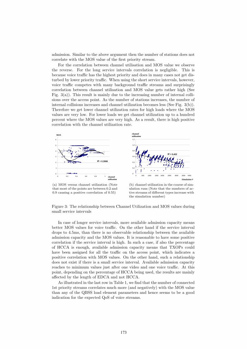
admission. Similar to the above argument then the number of stations does notcorrelate with the MOS value of the first priority stream.
For the correlation between channel utilisation and MOS value we observethe reverse. For the long service intervals correlation is negligible. This isbecause voice traffic has the highest priority and does in many cases not get dis-turbed by lower priority traffic. When using the short service intervals, however,voice traffic competes with many background traffic streams and surprisinglycorrelation between channel utilisation and MOS value gets rather high (SeeFig. 3(a)). This result is mainly due to the increasing number of internal colli-sions over the access point. As the number of stations increases, the number ofinternal collisions increases and channel utilization becomes less (See Fig. 3(b)).Therefore we get lower channel utilization rates for high loads where the MOSvalues are very low. For lower loads we get channel utilization up to a hundredpercent where the MOS values are very high. As a result, there is high positivecorrelation with the channel utilization rate.
channel utilisation
Simulation #
R2 = 0,422
0
0,2
0,4
0,6
0,8
1,0
1,2
0 500 1000 1500 2000 2500 3000 3500 4000
R2 = 0,3068
0
1
2
3
4
5
6
0 0,2 0,4 0,6 0,8 1 channel utilisation
MOS
(a) MOS versus channel utilization (Notethat most of the points are between 0.2 and0.9 causing a positive correlation of 0.55)
channel utilisation
Simulation #
R2 = 0,422
0
0,2
0,4
0,6
0,8
1,0
1,2
0 500 1000 1500 2000 2500 3000 3500 4000
R2 = 0,3068
0
1
2
3
4
5
6
0 0,2 0,4 0,6 0,8 1 channel utilisation
MOS
(b) channel utilization in the course of sim-ulation runs (Note that the numbers of ac-tive streams of different types increase withthe simulation number)
Figure 3: The relationship between Channel Utilization and MOS values duringsmall service intervals
In case of longer service intervals, more available admission capacity meansbetter MOS values for voice traffic. On the other hand if the service intervaldrops to 4.5ms, than there is no observable relationship between the availableadmission capacity and the MOS values. It is reasonable to have some positivecorrelation if the service interval is high. In such a case, if also the percentageof HCCA is enough, available admission capacity means that TXOPs couldhave been assigned for all the traffic on the access point, which indicates apositive correlation with MOS values. On the other hand, such a relationshipdoes not exist if there is a small service interval. Available admission capacityreaches to minimum values just after one video and one voice traffic. At thispoint, depending on the percentage of HCCA being used, the results are mainlyaffected by the length of EDCA and not HCCA.
As illustrated in the last row in Table 1, we find that the number of connected1st priority streams correlates much more (and negatively) with the MOS valuethan any of the QBSS load element parameters and hence seems to be a goodindication for the expected QoS of voice streams.
173

4.2 Video Traffic
Because we do not have a metric like MOS defined for video traffic streams,we are going to give the correlations of the information elements with delay,jitter and loss rates of the video traffic streams. In fact, as given in Table 2, theresults are very unstable for video traffic. If the traffic combination changes theresults change also. Nevertheless the sign of the correlation is constant. Thedelay and the number of stations correlate positively, as expected.
Since voice traffic has higher priority than video traffic, the number of voicetraffic streams increases the delay of video traffic directly. Additionally, videotraffic streams affect each other more than all the other traffic streams, becausevideo packets come more often and are larger. This causes a positive correlationbetween station count and delay. If the number of traffic streams associated withthe access point increases, the schedule of the HC becomes more stable andtherefore the jitter values decrease, which results in negative correlation. Thecorrelation with the loss rate is more stable compared to others, which can beexplained in a straightforward manner. On the other hand, channel utilizationand available admission capacity shows nearly no correlation with delay, jitteror loss rates.
Table 2: Correlations of video traffic; SI and HCCA percentage versus QBSSload elements and video traffic number
4.5 ms SI 50ms SIDelay Jitter Loss Delay Jitter Loss
40% HCCAStation Count -0.11 0.08 0.22 0.23 -0.23 0.22Channel Util. -0.21 0.05 -0.40 -0.05 -0.14 -0.06Avail. Adm.C. -0.23 0.59 0.68 -0.02 0.07 -0.022st priority # 0.69 -0.37 0.11 0.90 -0.71 0.89
80% HCCAStation Count -0.11 0.08 0.22 0.23 -0.23 0.22Channel Util. -0.21 0.05 -0.40 -0.05 -0.14 -0.06Avail. Adm.C. -0.23 0.59 0.68 -0.02 0.07 -0.022st priority # 0.69 -0.37 0.11 0.90 -0.71 0.89
98% HCCAStation Count 0.12 0.01 0.15 0.26 -0.15 0.29Channel Util. -0.18 0.10 -0.18 -0.09 -0.07 0.23Avail. Adm.C. 0 -0.02 0 0.13 0.04 -0.192st priority # 0.57 0.07 0.51 0.72 -0.81 0.83
The effect of the number of video traffic streams has mostly a high correlationwith delay, jitter and loss rates of the video traffic. This is due to the fact thatvideo traffic streams are relatively heavy loaded and constitute the main channelutilization. If the service interval is small, at most one video traffic can receiveTXOP and the remaining use the contention period. Because the contentionperiod is short and video packets come very often, the bandwidth reserved tothe video traffic is not enough and the loss rate increases suddenly. The jitterrate drops because the video packets coming very often allow a self repeatingschedule keeping delays nearly constant. But this does not have any importanceif the service interval is low, because the loss rate increases very fast making itimpossible to have more than two video traffic streams with an acceptable levelof QoS.
174
If the service interval is large and the time reserved for contention free periodis long, TXOPs given at the beginning of the service interval do not fully utilisethe amount of time reserved for scheduling which results the start of contentionperiod. Within the contention period, as the number of voice streams increases,the loss rate increases due to collisions and delay increases as well. On the otherhand longer delays achieve saturation, decreasing the variation in delay.
5 Evaluation of Results and Enhancement Rec-ommendation
The results of the Sections 4.1 and 4.2 show that the load element parame-ters channel utilization and available admission capacity are capable of givingmeaningful information in some of the parameter combinations because theyare moderately correlated with the metric of interest (MOS or delay, jitter andloss rates) in these cases. However this information is not reliable because itdepends on many other variables and is not stable. The station count is in noneof the cases a reliable source of information to estimate the expected QoS overan access point as there is no observed correlation bigger than -0.30. Such a lowcorrelation cannot be regarded as a source of information in decision making.Even more so since there is another parameter, the number of streams belongingto the respective priority class, that correlates much stronger.
In fact the number of traffic streams in each priority should definitely givean idea about the expected QoS, because in most cases, the number of any kindof traffic that can be transmitted over an access point has a maximum value andthis depends on the standard being used. For 802.11b the maximum numberof voice calls using G.711 codec is about 5 which can further be optimized to 7with more efficient algorithms [13]. For this reason we also compared the corre-lation between the number of traffic streams in each priority class and the QoSindicator values (MOS, delay, jitter and loss rates). The correlations betweenthe number of traffic streams using the first priority and the QoS indicators canbe found in Table 1 and the second priority can be found in Table 2. As itcan be observed, the correlations reach up to -0.9 for some of the cases. Exceptfor the correlation between jitter and the number of second priority traffic, themagnitude of the correlations is significantly higher than what we had for theload element parameters. Hence, it is worth having this additional informationin the QBSS load element which does not bring a considerably extra load tothe beacon frame. An extension of the current draft with the number of trafficusing different priority levels can ease the choice procedure substantially.
6 Conclusion
In this paper, we presented the QBSS load element and its use in the contextof 802.11e. Our simulation results showed that choosing a QAP based uponthe fields of the received QBSS load element fields, does not always lead to anassociation with the best available access point.
In order to delineate the poorness of the QBSS load element information, welisted the results of the correlation between the QBSS load element parametersand QoS factors like delay, jitter and loss rate. We showed that, in most of
175

the cases the correlation is very low and unfortunately even the sign of thecorrelation can change if one uses a different set of parameters.
We observed that in all cases with decreasing HCCA percentage, the deci-sion accuracy improved significantly supporting our claim that the HCCA bringsextra irregularity and complexity to the new standard. We conclude that, de-pending on the internal configuration of the QAP, meaning the settings of the802.11e relevant parameters, the provided network service cannot be boundbarely on the load information.
Although we presented two of the most important parameters affecting theperformance of 802.11e, incorporating more parameters into the decision pro-cess, for instance considering the number of traffic streams in different priorities,can improve the accuracy of the decision. We are going to analyse other param-eters of the TSPEC like surplus bandwidth allowance and delay bound, whichwill be included in our next study.
References[1] D. Chalmers, M. Sloman, A Survey Of Quality Of Service In Mobile Computing
Environment. IEEE Communications Surveys, pages 1-10, Second Quarter 1999.
[2] NS software and documentation is available at the following site:http://www.isi.edu/nsnam/ns/
[3] P.Ansel et a.l., ”An Efficient Scheduling Scheme for IEEE 802.11e”, conferenceproceedings, WiOpt, Modeling and Optimization in Mobile, Ad Hoc and WirelessNetworks, Cambridge, UK, March 2004.
[4] G. Boggia et a.l., ”Feedback based bandwidth allocation with call admission con-trol for providing delay guarantees in IEEE 802.11e networks”, Computer Com-munications, Elsevier, 28(3):325-337, February 2005.
[5] Sunghyun Choi, ”Protection and guarantee for voice and video traffic in IEEE802.11e wireless LANs”, IEEE Conference on Computer Communications, pp.0-0,Mar. 2004
[6] IEEE 802.11 WG, Draft Supplement to Part 11: Wireless Medium Access Con-trol (MAC) and physical layer (PHY) specifications: Amendment 7: MediumAccess Control (MAC) Enhancements for Quality of Service (QoS), IEEE Std802.11e/D9.0, August 2004.
[7] Zhang Q. et a.l., Efficient mobility management for vertical handoff betweenWWAN and WLAN. IEEE Communications, 41 (11) (2003) 102–108.
[8] K. Murray, D. Pesch, ”Intelligent Network Access and Inter-System HandoverControl in Heterogeneous Wireless Access Networks for Smart Space Environ-ments”, conference proceedings, 1st IEEE International Symposium on WirelessCommunication Systems, Mauritius, September 2004
[9] http://www-sop.inria.fr/planete/qni/fhcf/
[10] ITU-T Rec. G.107. The E-Model, a Computational Model for Use in TransmissionPlanning. International Telecommunication Union, CHGenf, 2002.
[11] ITU-T Rec. P.85. A Method for Subjective Performance Assessment of the Qualityof Speech Voice Output Devices. International Telecommunication Union, CH-Genf, 1994.
[12] Zhu, H. and Chlamtac, I, ”An Analytical Model for IEEE 802.11e EDCF Differ-ential Services”, IEEE ICCCN, Dallas, October 2003.
[13] Coupechoux, M. et a.l.,”Voice over IEEE 802.11b Capacity”, ITC Specialist Sem-inar on Performance Evaluation of Wireless and Mobile Systems, Antwerp, 2004.
176
Performance Evaluation of Processor Allocation Strategies in the 2-Dimensional Mesh Network
S. Bani-Mohammad1, M. Ould-Khaoua1 and I. Ababneh2
1Department of Computing Science University of Glasgow
Glasgow G12 8RZ UK
Email: {saad, Mohamed}@dcs.gla.ac.uk
2Department of Computing Science Al al-Bayt University
Mafraq, Jordan Email: [email protected]
Abstract
Contiguous allocation of parallel jobs usually suffers from the degrading effects of fragmentation as it requires that the allocated processors be contiguous and have the same topology as the network connecting these processors. In this paper, two non-contiguous processor allocation strategies, referred to as Paging and Greedy-Available respectively, are suggested for the 2D mesh network, and are compared using simulation against the well-known contiguous First Fit strategy. The results reveal that the proposed non-contiguous strategies exhibit superior performance properties despite the added contention that results from non-contiguity.
Keywords: Multicomputers, Fragmentation, Scheduling Effectiveness, Turnaround Time, External Message Interference, Dispersal Ratio, Performance Comparison, Simulation.
1. Introduction In a multicomputer, processor allocation is responsible for selecting the set of processors on which parallel jobs are executed. Most strategies employed in a multicomputer are based on contiguous allocation, where the processors allocated to a parallel job are physically contiguous and have the same topology as the network connecting the processors [3, 9, 10, 12]. These strategies often result in high external processor fragmentation, as has been shown in [12]. External fragmentation occurs when there are free processors sufficient in number to satisfy the number requested by a parallel job, but they are not allocated to it because the free processors are not contiguous or they do not have the same topology as the network topology connecting these processors.
Several studies have attempted to reduce such fragmentation [2, 4, 10]. One solution suggested is non-contiguous allocation [2, 10]. In such a strategy, a job can
177
execute on multiple disjoint smaller sub-networks rather than always waiting until a single sub-network of the requested size is available. Although non-contiguous allocation increases message contention in the network, lifting the contiguity condition is expected to reduce processor fragmentation and increase processor utilization [10]. Folding has also been proposed for the 2D mesh [2, 4]. Folding permits applications to execute on fewer processors than they have requested, when necessary. This could improve the performance of contiguous and non-contiguous allocation, as demonstrated in [2, 4]. The problem with folding is that it requires that jobs be able to execute on a number of processors determined at load time.
Existing research studies [2, 4, 10] on both contiguous and non-contiguous allocation have been carried out in the context of the 2D mesh. The 2D mesh has been used as the underlying network in a number of practical and experimental parallel machines, such as iWARP [1] and Delta Touchstone [7]. In this study, we investigate the performance merits of non-contiguous allocation for reducing processor fragmentation on the 2D mesh and compare its performance to that of the contiguous allocation. To do so, two non-contiguous allocation strategies, notably Greedy-Available and Paging, are suggested. The Greedy-Available and Paging strategies combine the desirable features of both contiguous and non-contiguous allocation strategies. The Greedy-Available strategy only allocates jobs non-contiguously when external fragmentation occurs (i.e., when contiguous allocation fails to allocate an incoming job). In the Paging strategy, a request for a given number of processors is satisfied by the first free pages in a row major scan of the mesh, and some degree of contiguity is maintained through the nature of the row major scan. The performance of both strategies will be compared against the existing well known contiguous First Fit [12] under contention and contention-free communication models. The First Fit strategy allocates an incoming job to the first available sub-mesh that is found [12]. In this study, First Fit has been used to represent the contiguous class of strategies as it has been found to perform well [12]. In order to make comparison fair and realistic, we will consider the contention model to assess the effects of contention on the performance of non-contiguous allocation when comparing against the First fit strategy.
The rest of the paper is organised as follows. Section 2 contains a brief summary of allocation strategies previously proposed for 2D mesh. Section 3 contains the proposed non-contiguous allocation strategies. Section 4 compares the performance of the contiguous and non-contiguous allocation strategies. Section 5 concludes this study.
2. Related Work
Two Dimensional Buddy System (2DBS): The 2DBS allocation [8] applies to square mesh systems with power of two side lengths. Processors allocated to jobs also form square sub-meshes with power of two side lengths. If a job requests a sub-mesh of size ba× such that ba ≤ , the 2DBS allocates a sub-mesh of sizess× , where
( )( ) b,amaxlogs 2= . This strategy suffers from high fragmentation. Also, it cannot be used for non-square meshes and does not have complete sub-mesh recognition ability.
Frame Sliding (FS): The frame sliding strategy [9] searches for an appropriate allocation using a set of sequenced non-overlapping processor frames that cover the whole target mesh. It is assumed that arriving jobs request processor subsets of rectangular shape. Processor frames of the same side lengths as the requested sub-mesh are searched from left to right and from bottom to top. Jumps to successive frames are by the job's width and height. The goal of searching is to find a suitable
178

frame for allocation; i.e., all its processors are free and it is big enough to accommodate the allocation request. This process ends either with finding a suitable allocation or when all frames are scanned and no appropriate frame is found. A problem with this strategy is that it cannot recognise all free frames because the jumps are by the job's width and height [10]. In this strategy, the search process starts with the lowest leftmost available node. If processors in the currently examined frame are not all available, the frame is slide over the plane of the mesh to the next candidate frame, with horizontal and vertical strides equivalent to, respectively, the width and the length of the requested sub-mesh. The frame first slides horizontally from left to right until it exceeds the boundary of the mesh. At that point, a vertical slide takes place. Further sliding again takes place horizontally from right to left, and so on. This strategy does not guarantee complete sub-mesh recognition, i.e., an available free sub-mesh can go undetected by the strategy [3].
First Fit (FF) and Best Fit (BF): The problem of missing an existing possible allocation explained above is solved using First Fit and Best Fit allocation strategies [12]. The free sub-meshes are scanned and First Fit allocates the first sub-mesh that is large enough to hold the job, whereas Best Fit allocates the smallest suitable sub-mesh. Bit arrays are used for scanning of available processors.
The above allocation strategies consider only contiguous regions for the execution of a job and are referred to as contiguous allocations. Distance of the communication path is expected to be minimized in contiguous allocations. Only messages generated by the same process are expected within a sub-mesh and therefore cause no interjob contention in the network. On the other hand, the restriction that jobs have to be allocated to contiguous processors reduces the chance of successfully allocating a job. It is possible for the mesh to fail to allocate a job while a sufficient number of processors are available [2], i.e., fragmentation are occurred in these strategies.
Hardware advances such as wormhole routing and faster switching techniques have made the communication latency less sensitive to the distance between the communicating nodes. This makes allocating a job to non-contiguous processors plausible. Allocation of jobs to non-contiguous nodes allows jobs to be executed without waiting if the number of available processors is sufficient [2]. In the next paragraphs, we present non-contiguous allocation strategies that have been proposed in previous studies [2, 10, 11].
Random: The random allocation is a straightforward strategy in which a request for a given number of processors is satisfied with a number of processors selected randomly [10]. Both internal and external fragmentations are eliminated since all jobs are assigned exactly the requested number of processors if available. Because no contiguity is enforced under this strategy, we would expect much communication interference amongst jobs.
Naive: In the naive algorithm [11], a request for a given number of processors is allocated to the first free nodes found in a row major scan.
Multiple Buddy System (MBS): The MBS is an extension of the 2D buddy strategy. The mesh is divided into non-overlapped square sub-meshes with side lengths equal to the powers of two upon initialization. The number of processors,p ,
requested by an incoming job is factorized into a base of four representation of
( )
∑=
××plog
i
iiid
4
0
22 , where 30 ≤≤ id . The request is then allocated to the mesh
according to the factorized number in which id number of ii 22 × blocks is required.
If a required block is unavailable, MBS recursively searches for a bigger block and
179
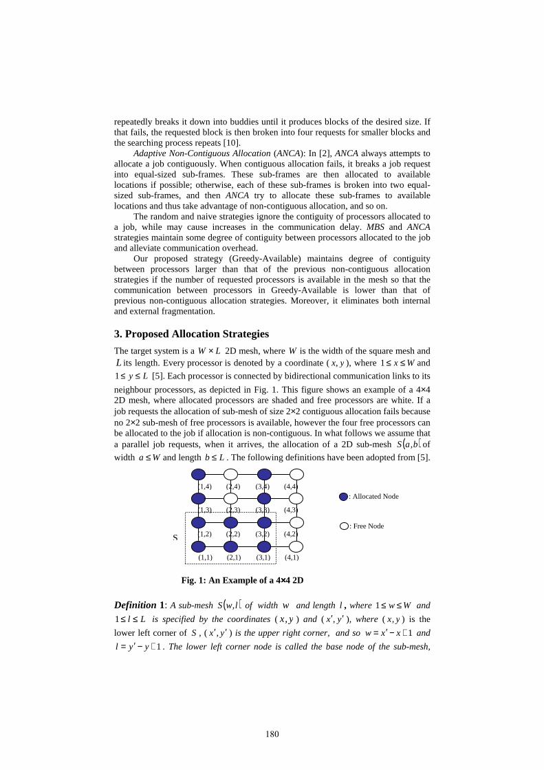
repeatedly breaks it down into buddies until it produces blocks of the desired size. If that fails, the requested block is then broken into four requests for smaller blocks and the searching process repeats [10].
Adaptive Non-Contiguous Allocation (ANCA): In [2], ANCA always attempts to allocate a job contiguously. When contiguous allocation fails, it breaks a job request into equal-sized sub-frames. These sub-frames are then allocated to available locations if possible; otherwise, each of these sub-frames is broken into two equal-sized sub-frames, and then ANCA try to allocate these sub-frames to available locations and thus take advantage of non-contiguous allocation, and so on.
The random and naive strategies ignore the contiguity of processors allocated to a job, while may cause increases in the communication delay. MBS and ANCA strategies maintain some degree of contiguity between processors allocated to the job and alleviate communication overhead.
Our proposed strategy (Greedy-Available) maintains degree of contiguity between processors larger than that of the previous non-contiguous allocation strategies if the number of requested processors is available in the mesh so that the communication between processors in Greedy-Available is lower than that of previous non-contiguous allocation strategies. Moreover, it eliminates both internal and external fragmentation.
3. Proposed Allocation Strategies
The target system is a LW × 2D mesh, where W is the width of the square mesh and L its length. Every processor is denoted by a coordinate (yx, ), where Wx ≤≤1 and
Ly ≤≤1 [5]. Each processor is connected by bidirectional communication links to its
neighbour processors, as depicted in Fig. 1. This figure shows an example of a 4×4 2D mesh, where allocated processors are shaded and free processors are white. If a job requests the allocation of sub-mesh of size 2×2 contiguous allocation fails because no 2×2 sub-mesh of free processors is available, however the four free processors can be allocated to the job if allocation is non-contiguous. In what follows we assume that a parallel job requests, when it arrives, the allocation of a 2D sub-mesh ( )b,aS of
width Wa ≤ and length Lb ≤ . The following definitions have been adopted from [5].
Definition 1: A sub-mesh ( )l,wS of width w and length l, where Ww ≤≤1 and
Ll ≤≤1 is specified by the coordinates ( y,x ) and ( yx ′′, ), where ( y,x ) is the
lower left corner of S , ( y,x ′′ ) is the upper right corner, and so 1+−′= xxw and
1+−′= yyl . The lower left corner node is called the base node of the sub-mesh,
(1,1) (2,1) (3,1) (4,1)
(1,3) (2,3) (3,3) (4,3)
(1,4) (2,4) (3,4) (4,4)
Fig. 1: An Example of a 4××××4 2D
S (1,2) (2,2) (3,2) (4,2) : Free Node
: Allocated Node
180

whereas the upper right corner node is the end node. For example (1, 1, 3, 2) represents the 3 × 2 sub-mesh S in Fig. 1. The base node of the sub-mesh is (1, 1), and its end node is (3, 2).
Definition 2: The size of ),( lwS is lw× .
Definition 3: An allocated sub-mesh is one whose processors are all allocated to a parallel job.
Definition 4: A free sub-mesh is one whose processors are all unallocated.
Definition 5: A suitable sub-mesh ),( yxS is a free sub-mesh that satisfies the
conditions: ax ≥ and by ≥ assuming that the allocation of ),( baS is requested.
In this study, it is assumed that parallel jobs are selected for allocation and execution using FCFS strategy. This strategy is chosen because it is fair and it is widely used in other studies [2, 3, 5, 10] and because this research deals with the allocation problem. In the next two sub-sections, we describe the two non-contiguous allocation strategies.
3.1 Greedy-Available Strategy
In the Greedy-Available strategy, when a parallel job is selected for allocation a sub-mesh suitable for the entire job is searched for. If such sub-mesh is found it is allocated to the job and allocation is done. Otherwise, the largest free sub-mesh that can fit inside ( )b,aS is allocated. Then, the largest free sub-mesh whose side lengths
do not exceed the corresponding side lengths of the previous allocated sub-mesh is searched for and allocated if this does not result in allocating more processors than
ba× . This last step is repeated until ba× processors are allocated. This allocation process is implemented by the algorithm bellow, illustrated in
Fig. 2. Note that allocation always succeeds if the number of free processors ba×≥ , and scanning for free sub-meshes uses the First Fit strategy. Moreover, it can be noticed that this strategy maintains some contiguity by allocating large sub-meshes.
Fig. 2: Outline of the Greedy-Available allocation algorithm
Procedure Greedy-Available_Submesh_Allocation (a, b):
Total_allocated = 0; Job_Size = a×b
Step 1. If (number of free processors < Job_Size) return failure
Step 2. If (there is a free S (x, y) suitable for S(a, b)) allocate the first one (i.e., First Fit) and return success
Step 3. aa=a and bb=b
Step 4. Subtract 1 from max(aa, bb) if max > 1
Step 5. If (Total _allocated+ aa×bb > Job_Size) go to step 4
Step 6. If (there is a free S(aa, bb)) allocate it using First Fit,Total_allocated = Total_allocated + aa×bb
Step 7. If (Total_allocated = Job_Size) return success else go to step 5 End.
181

3.2 Paging Strategy
The entire 2D mesh is divided into pages that are sub-meshes with equal sides’ length
of index_size2 , where index_size is a positive integer. A page is the allocation unit.
The pages are indexed according to the row-major indexing scheme, as illustrated in Fig. 3. Busy arrays are used for scanning of available processors.
If the number of free pages is greater than or equal to the allocation request the
pages are scanned starting with page zero until the needed number of free pages is allocated. A paging strategy is denoted as Paging( indexsize_ ). For example,
Paging(2) means that the pages are 4×4 sub-mesh. The number of pages a job requests is computed using the equation:
( ) PsizebaPrequest /×= (1)
where Psizeis the size of the pages, and a and bare again the side lengths of the requested sub-mesh. This allocation process is implemented by the Paging algorithm, illustrated in Fig. 4.
Fig. 4: Outline of the Paging allocation algorithm
The time taken by this algorithm to scan for and allocate free pages is in the
worst case bounded from above by LW × ; that is, its time complexity is in ( )LWO × . Paging suffers from internal fragmentation when size_index > 0. The
internal fragmentation of running jobs is computed using:
Internal_Fragmentation = ∑jobs
rocessorsAllocate_P
ssorsLost_Proce (2)
Procedure Paging_Allocation (a, b):
Pside=2size_index; Psize=Pside×Pside; Mesh-Size = (W× L)/Psize;
Prequest = (a× b)/Psize
Step 1. If (number of free pages < Prequest) return failure else go to step 2
Step 2. Allocate the first Prequest free pages to the job, and return success End.
Fig. 3: Row-Major indexing
5 6
2
8
14
10
12
4
0
15
9
1 3
7
11
13
182
where ssorsLost_Proce for a parallel job that requests zeProgram_Si processors,
but is allocated PagesAllocatedofNumber ___ is calculated using:
Size_ogramPrPsizepages_Allocated_of_NumberocessorsPr_Lost −×= (3)
To illustrate this, consider a paging strategy with index_size =1, and suppose a
parallel job requests the allocation of a 3×3 sub-mesh. When allocation is carried out for the job it is allocated 3 pages (12 processors). Since only 9 processors are needed there is internal fragmentation of 3/12.
4. Performance Evaluation Simulation has been used to evaluate the proposed allocation algorithms and compare them to First Fit for various mesh sizes and system loads. The main performance parameters used are the mean turnaround times of jobs and the mean scheduling effectiveness eS . The scheduling effectiveness measures the ability of the allocation
algorithms to avoid processor fragmentation [6]. At simulation time t the scheduling effectiveness is defined by the following equation:
( ) ( ) ( )( )tPPtPtS dae ,min/= (4)
where aP is the number of allocated processors, P the number of processors in the
multicomputer, and dP the total processor demand of the jobs in the multicomputer,
running or waiting. For example, if 100=P , 140=dP and 80=aP the scheduling
effectiveness is 0.8 and processor fragmentation is 0.2 (1.0 minus 0.8). However, if 40=dP and 40=aP the scheduling effectiveness is 1.0 and fragmentation is 0.0.
The turnaround time is the time that a parallel job spends in the mesh, from arrival to departure. The mean scheduling effectiveness is taken over the entire simulation time, and the mean turnaround time is the average turnaround time taken for all completed jobs.
Every simulation run completes the execution of 500 parallel jobs. The runs are repeated enough times so that the mean performance values obtained have relative errors that do not exceed 5% under a confidence level of 95%. The side lengths of the sub-meshes requested by programs are uniformly distributed over the range from 1 to the mesh side length. Unless it is other specified the target mesh has equal sides of 32 processors.
As in previous studies [5, 6], we assume that programs arrive from a Poisson source at a rate of λ jobs per time unit. The rate is computed using the equation
( )eTN/PL ××=λ , where N is the mean number of processors requested by jobs,
eT their mean execution time, and L is the system load. The execution times are
exponentially distributed with 1=eT time unit.
The performance of non-contiguous allocation depends on the contention that results from external message interference. The messages of two or more jobs may need to use the same communication link simultaneously. Therefore, this study uses two contention models. The first is the contention-free model, which ignores external message interference. The second is the contention model, where external message interference is modelled. The execution time of a job is not changed if the sub-mesh it is allocated is contiguous. However, if allocation is non-contiguous the execution time of the job is changed using the following formula, proposed by Chang and Mohapatra
183

[2].
TimeExecutionInitialTimeExecutionNew __60.1__ ×= (5)
Figs. 5 and 6 show the mean scheduling effectiveness achieved by the non-contiguous allocation strategies and the contiguous allocation strategy First Fit under the two contention models. It can be noticed in the figures that Paging(0), Paging(1) and Greedy-Available are better than first fit for most system loads. Moreover, they are highly superior under medium to high loads. This is due to the fact that contiguous policies, represented by first fit, produce high external fragmentation under such loads. The scheduling effectiveness of first fit is high when the load is low because it is highly likely that a suitable contiguous sub-mesh is available for allocation to a job when it arrives to the mesh. The poor performance of Paging(2) and Paging(3) can be easily noticed. It is due to internal fragmentation caused by their large pages, respectively, (4×4 processors) and (8×8 processors) compared to the size of the mesh. It can also be noticed that the performance of Paging(0), Paging(1) and Greedy-Available strategies differs by little using contention-free model. Also, you can notice that Greedy-Available is better than Paging(0) and Paging(1) using contention model.
0.3
0.4
0.5
0.6
0.7
0.8
0.9
1
0.001 0.101 0.201 0.301 0.401 0.501 0.601 0.701
Load
Mea
n S
ched
ulin
g E
ffec
tivn
ess
First Fit
Available
Paging(0)
Paging(1)
Paging(2)
Paging(3)
Fig. 5: Mean scheduling effectiveness for First Fit and the non-
contiguous strategies using the contention-free model in a 32×32 mesh.
0.3
0.4
0.5
0.6
0.7
0.8
0.9
1
0.001 0.101 0.201 0.301 0.401 0.501 0.601
Load
Mea
n S
ched
ulin
g E
ffec
tivn
ess
First Fit
Available
Paging(0)
Paging(1)
Paging(2)
Paging(3)
Fig. 6: Mean scheduling effectiveness for First Fit and the non-
contiguous strategies using the contention model in a 32×32 mesh.
184

Figs. 7 and 8 show the mean turnaround times of First Fit and non-contiguous allocation strategies using both the contention-free and contention models. As can be seen in Fig. 7, Paging(0), Paging(1), Paging(2), and Greedy-Available perform much better than first fit using contention-free model. On the other hand, the performance of contiguous first fit strategy is superior to non-contiguous strategy Paging(3) for most system loads using both the contention-free and contention models, this is due to internal fragmentation caused by its large pages (8×8 processors). Moreover, the performance of Paging(0), Paging(1), and Greedy-Available is almost identical, and is better than Paging(2) is substantially better than Paging(3) using contention-free model. The poor performance of Paging(3) is due to its large pages size. This produces poor scheduling effectiveness as revealed in Figs. 5 and 6. It can also be noticed that, and as revealed in Fig. 8, Greedy-Available perform much better than first fit and Paging strategies for most system loads using contention model.
1
6
11
16
21
26
0.0001 0.1001 0.2001 0.3001 0.4001 0.5001 0.6001 0.7001
Load
First Fit
Available
Paging(0)
Paging(1)
Paging(2)
Paging(3)
Fig. 7: Mean turnaround times for First Fit and the non-contiguous
strategies using the contention-free model in a 32×32 mesh.
1
6
11
16
21
26
0.0001 0.1001 0.2001 0.3001 0.4001 0.5001 0.6001
Load
Mea
n T
urn
arro
un
d T
ime
First Fit
Available
Paging(0)
Paging(1)
Paging(2)
Paging(3)
Fig. 8: Mean turnaround times for First Fit and the non-contiguous
strategies using the contention model in a 32×32 mesh.
As expected, the advantage of non-contiguous allocation over contiguous allocation is lower when contention is modelled, however it remains substantial. We have also carried out simulation experiments for other mesh sizes, but this did not change the relative performance of the allocation strategies.
In addition to the scheduling effectiveness and turnaround times, we have measured two other performance parameters for the non-contiguous strategies. These
185

are the mean dispersal ratio and mean distance computed for all jobs. The dispersal ratio is a measure of the degree to which the sub-meshes allocated to a job are dispersed over the entire mesh. The higher the dispersal ratio the more likely it is that the job's messages will travel through nodes allocated to other jobs, potentially causing more contention in the interconnection network [10]. The dispersal ratio is defined as follows
Dispersal ratio =∑ ×+−×+−
jobsba
YstartYendXstartXend
)(
)1()1( (6)
where ( )YstartXstart, is the base of the smallest sub-mesh that includes all
processors allocated to a job, and ( )YendXend, is its end. The values a and bare the
side lengths of the parallel job's request. The mean distance for a parallel job is defined as the sum of the distances
amongst all pairs of processors allocated to it. The distance is defined as follows
Distance = ∑ ×−+−
jobsba
yyabsxxabs
)(
))(())(( 11 (7)
where , yx, y, x )( 11 are the coordinates of the pairs of the processors allocated to a
job. The values a and b are the side lengths of the parallel job's request. This distance is an indicator of contention; that is, the higher the distance the higher contention is likely to be.
Fig. 9 shows the mean dispersal ratio for the two non-contiguous strategies that yields the best performance (Greedy-Available and Paging(0)). The results reveal that Greedy-Available and Paging(0) have the same dispersal ratio for lighter loads (less than 0.3). However, the dispersal ratio of Greedy-Available is higher for high loads (greater than about 0.4).
Fig. 10 displays the mean distance calculated for all jobs in Paging(0) and Greedy-Available. As can be seen in the figure, the mean distance for Greedy-Available is less than that of Paging(0) for loads less than 0.6 approximately, while the mean distance for Greedy-Available is equivalent to that of Paging(0) for loads greater than 0.6 approximately. This suggests that it is expected that Paging(0) and Greedy-Available yield comparable performance across all loads. This conclusion is compatible with the values of the mean scheduling effectiveness and the mean turnaround times shown above. These results suggest that the mean distance is a better performance parameter than the dispersal ratio so that Greedy-Available is better than Paging(0).
0.5
1
1.5
2
2.5
3
3.5
4
4.5
5
0.1 0.2 0.3 0.4 0.5 0.6 0.7
Load
Mea
n D
isp
ersa
l Rat
io
Available
Paging(0)
Fig. 9: Mean dispersal ratio for Paging(0) and Greedy-Available
using the contention model in a 32×32 mesh.
186

3000
3500
4000
4500
5000
0.1 0.2 0.3 0.4 0.5 0.6 0.7 0.8 0.9
Load
Mea
n D
ista
nce
Available
Paging(0)
Fig. 10: Mean distance for Paging(0) and Greedy-Available using the contention model in a 32×32 mesh.
5. Conclusions This study has investigated the performance merits of non-contiguous allocation in the 2D mesh. To this end, two non-contiguous allocation strategies, notably Greedy-Available and Paging, have been presented. The performance of both strategies has been compared against the existing contiguous First Fit under contention and contention-free communication models. The aim of using the contention model is to assess the effects of contention on the performance of non-contiguous allocation. Simulation results have revealed that non-contiguous allocation greatly improves performance despite the additional message contention inside the network that results from the interference among the messages of different jobs. Non-contiguous allocation produces superior utilization than its contiguous allocation counterpart. Results have also shown that when pages are small the proposed strategies exhibit good performance levels. However, when the pages are large the performance of Paging degrades because of internal fragmentation. An advantage of paging over Greedy-Available is that it can easily be implemented efficiently. Its execution time complexity is ( )LWO × .
As a continuation of this research in the future, it would be interesting to evaluate the performance of the contiguous and non-contiguous allocation strategies with different scheduling approaches. It would be also interesting to assess of the existing allocation strategies on a practical multicomputer.
References [1] C. Peterson, J. Sutton, P. Wiley, iWARP: a 100-MPOS VLIW
microprocessor for multicomputers, IEEE Micro, vol. 11, no. 13, 1991. [2] C.-Y. Chang, P. Mohapatra, Performance improvement of allocation schemes
for mesh-connected computers, Journal of Parallel and Distributed Computing, vol. 52, no. PC981459, pp. 40-68, 1998.
[3] G.-M. Chiu, S.-K. Chen, An efficient submesh allocation scheme for two-dimensional meshes with little overhead, IEEE Transactions on Parallel & Distributed Systems, vol. 11, no. 5, pp. 471-486, 1999.
[4] I. Ababneh, F. Fraij, Folding contiguous and non-contiguous space sharing policies for parallel computers, Mu’tah Lil-Buhuth wad-Dirasat, Natural and Applied Sciences Series, vol. 16, no. 3, pp. 9-34, 2001.
[5] I. Ababneh, S. Bani Mohammad, Noncontiguous Processor Allocation for
187
Three-Dimensional Mesh Multicomputers, AMSE Advances in Modelling & Analysis, vol. 8, no. 2, pp. 51-63, 2003.
[6] I. Ismail, J. Davis, Program-based static allocation policies for highly parallel computers, Proc. IPCCC 95, IEEE Computer Society Press, pp. 61-68, 1995.
[7] Intel Corporation, A Touchstone DELTA system description, 1991. [8] K. Li, K.-H. Cheng, A Two-Dimensional Buddy System for Dynamic
Resource Allocation in a Partitionable Mesh Connected System, Journal of Parallel and Distributed Computing, vol. 12, no. 1, pp. 79-83, 1991.
[9] P.-J. Chuang, N.-F. Tzeng, Allocating precise submeshes in mesh connected systems, IEEE Transactions on Parallel and Distributed Systems, vol. 5, no. 2, pp. 211-217, 1994.
[10] V. Lo, K. Windisch, W. Liu, B. Nitzberg, Non-contiguous processor allocation algorithms for mesh-connected multicomputers, IEEE Transactions on Parallel and Distributed Systems, vol. 8, no. 7, pp. 712-726, 1997.
[11] V. Lo, K. Windisch, W. Liu, B. Nitzberg, Non-contiguous processor allocation algorithms for distributed memory multicomputers, Proceedings of Supercomputing 94, pp. 227-236, 1994.
[12] Y. Zhu, Efficient processor allocation strategies for mesh-connected parallel computers, Journal of Parallel and Distributed Computing, vol. 16, no. 4, pp. 328-337, 1992.
188

Fault Detection Mechanisms for Autonomic Distributed Applications.
E.Grishikashvili Pereira1, R. Pereira2, A. Taleb-Bendiab2
Abstract
Autonomic computing includes a range of desirable properties, which are best achieved through middleware support. One of these properties is self-healing, the ability that systems may have to reconfigure themselves following the failure of some component. Recently, we have witnessed the development of models to provide middleware-based support for self-healing, service oriented distributed systems. The On-Demand Assembly and Delivery (OSAD) proposed previously by the authors consists of a number of components associated with fault-detection and fault-recovery. In this paper, we consider the performance impact of a number of fault-detection mechanisms, including pre-emptive detection and on-use detection. 1. Introduction There is a growing body of knowledge associated with techniques related to self-healing [1] [2] [3] [4] . Although to a certain extent self-healing is not yet well defined in terms of scope and architectural models, it has received increased attention lately. A short definition of a self-healing system is a system that is capable of performing a reconfiguration step in order to recover from a permanent fault. The following requirements are likely to be relevant to most self-healing systems [5]: adaptability, dynamicity, awareness, autonomy, robustness, distributability, mobility and traceability. In addition, it is also essential that self-healing systems have strong monitoring abilities. Self-healing properties are particularly useful in dynamic systems, particularly distributed, service oriented systems, where new services may be added and removed from the network, leading to the need for applications to reconfigure themselves [6] [7]. Ideally, such reconfiguration steps would be carried out without user intervention. Distributed service oriented systems provide application developers with the ability to build applications using services provided by other systems across available in a network. Such arrangement requires some form of organisation, normally involving a look up service, which contains information about all services that are available in the network. Applications wishing to use a networked service would carry out a search on the look up service and select, based on some criteria, the service that best matches its requirements. A well-known system based on distributed services is JINI, which provides some support for distributed service-oriented systems [8] [9].
1 Department of Computing and IS Edge Hill Uni. College, St. Helen’s Road, Ormskirk, L39 4QP, [email protected] 2 School of Computing and Mathematical Sciences Liverpool John Moores University, Byrom Street, Liverpool, L3 3AF, UK, [email protected]
189

This paper is organised as follows. Section 2 describes some relevant related work; section 3 provides an overview of the OSAD model architecture; section 4 describes fault detection mechanisms; section 5 describes the experiment and presents the results of the simulation; section 6 discusses the evaluation of the experiment and section 7 presents our conclusions. 2. Related Work In order to perform self-healing systems should have the ability to modify their own behaviour in response to changes in their environment, such as resource variability, changing user needs, mobility and system faults. The lifecycle of self-healing systems consists of five major elements [10]:
1. Runtime monitoring of a given target, be it the system itself or its system parts or others;
2. Exception Event detection, including: an event arising from a deviation from a given model, normal system states and/or behaviour;
3. Diagnosis, including: identification of events and the right course of action; 4. Generating a plan of change such as architectural transformation during a
software reconfiguration process; 5. Validation and enactment of a given change plan.
The monitoring and problem detection was described as one of the essential features of autonomic/self-healing systems in the report: “The Vision of Autonomic Computing” published by IBM [1]. Since then a number of architectural models for Self-Healing systems, based on monitoring, problem detection and repair have been developed. The use of architectural models as the centrepiece of model-based adaptation has been explored by Garlan et al. [11], where the architectural models are used for the runtime system’s monitoring and reasoning; for instance, to understand what the running system is doing in high level terms, detect when architectural constraints are violated, and reason about repair actions at the architectural level. The idea of distributed object system monitoring and supervision of a self-healing process is shared and extended in Reilly and colleagues work [12], in which an architecture and associated middleware services were developed to support dynamic instrumentation to detect abnormal systems’ states (events) and trigger and control a self-healing process thereby ensuring safety. Gross and colleagues from Columbia University [13] also agree that it is essential for self-healing systems to have strong system monitoring abilities. Their work “An Active Event Model for Systems Monitoring” is based on an intelligent event model called ActiveEvent. ActiveEvents build on conventional event concepts by augmenting raw and structural data with semantic information, thereby allowing recipients to be able to dynamically understand the content of new kinds of events. Two submodels of ActiveEvents are proposed: SmartEvents, which are lightweight XML structured events containing references to their syntactic and semantic models, and GaugeEvents, which are heavier but more flexible mobile agents. By classifying the events as lightweight and sophisticated it becomes easer to deal with system monitoring. 3. The OSAD model The On-demand Service Assembly and Delivery (OSAD) model [14] provides an abstract view of the relationship of the distributed components and services. The objective of the OSAD model is to organize the following issues in a uniform framework:
190
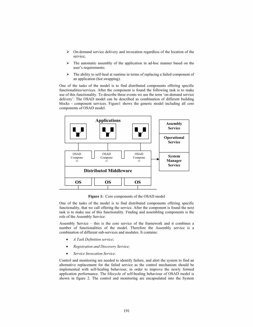
On-demand service delivery and invocation regardless of the location of the service;
The automatic assembly of the application in ad-hoc manner based on the user’s requirements;
The ability to self-heal at runtime in terms of replacing a failed component of an application (hot swapping).
One of the tasks of the model is to find distributed components offering specific functionalities/services. After the component is found the following task is to make use of this functionality. To describe these events we use the term ‘on-demand service delivery’. The OSAD model can be described as combination of different building blocks - component services. Figure1 shows the generic model including all core components of OSAD model.
Figure 1: Core components of the OSAD model
One of the tasks of the model is to find distributed components offering specific functionality, that we call offering the service. After the component is found the next task is to make use of this functionality. Finding and assembling components is the role of the Assembly Service:
Assembly Service – this is the core service of the framework and it combines a number of functionalities of the model. Therefore the Assembly service is a combination of different sub-services and modules. It contains:
• A Task Definition service;
• Registration and Discovery Service;
• Service Invocation Service.
Control and monitoring are needed to identify failure, and alert the system to find an alternative replacement for the failed service as the control mechanism should be implemented with self-healing behaviour, in order to improve the newly formed application performance. The lifecycle of self-healing behaviour of OSAD model is shown in figure 2. The control and monitoring are encapsulated into the System
OS OS OS
Distributed Middleware
OSAD Compone
nt
OSAD Compone
nt
OSAD Compone
nt
Applications Assembly
Service
Operational Service
System Manager Service
191

Manager, which is another core component of the OSAD model. The system manager is responsible for recovering the application from failure. Following failure detection, it notifies the assembly service that a replacement service should be found and selected amongst possible alternatives.
Figure 2: The lifecycle of self-healing behaviour in OSAD
4. Fault Detection Mechanisms Failure detection can be implemented in different ways, which can have considerable impact on the performance of the system. Two mechanisms that we put forward for consideration are: Pre-emptive detection and on-use detection. With pre-emptive detection, the service manager checks, on a regular basis, that each of the services associated with the application is alive. If a service fails to respond to the service manager, it is assumed that the service has failed and the recovery process is started and the service manager then notifies the assembly service. With the on-use detection, the service manager monitors locally the service requests and, if a request times-out, it is assumed that the service has failed and the recovery process is started and the service manager then notifies the assembly service. The performance considerations in this study relates to how these two mechanisms impact on service replacement waiting time and on network traffic. The notion of service replacement waiting time is important: It is the amount of time the application is prevented from using the service, because the service is found to have failed and is being replaced. The main advantage of the pre-emptive detection is that, as the service manager periodically polls the services, services may be found to be faulty prior to the moment when the application would wish to use them, therefore they can be replaced with zero replacement waiting time. The figure below shows the replacement waiting time for the on-use replacement mechanism, against the total number of services in used by the application:
192
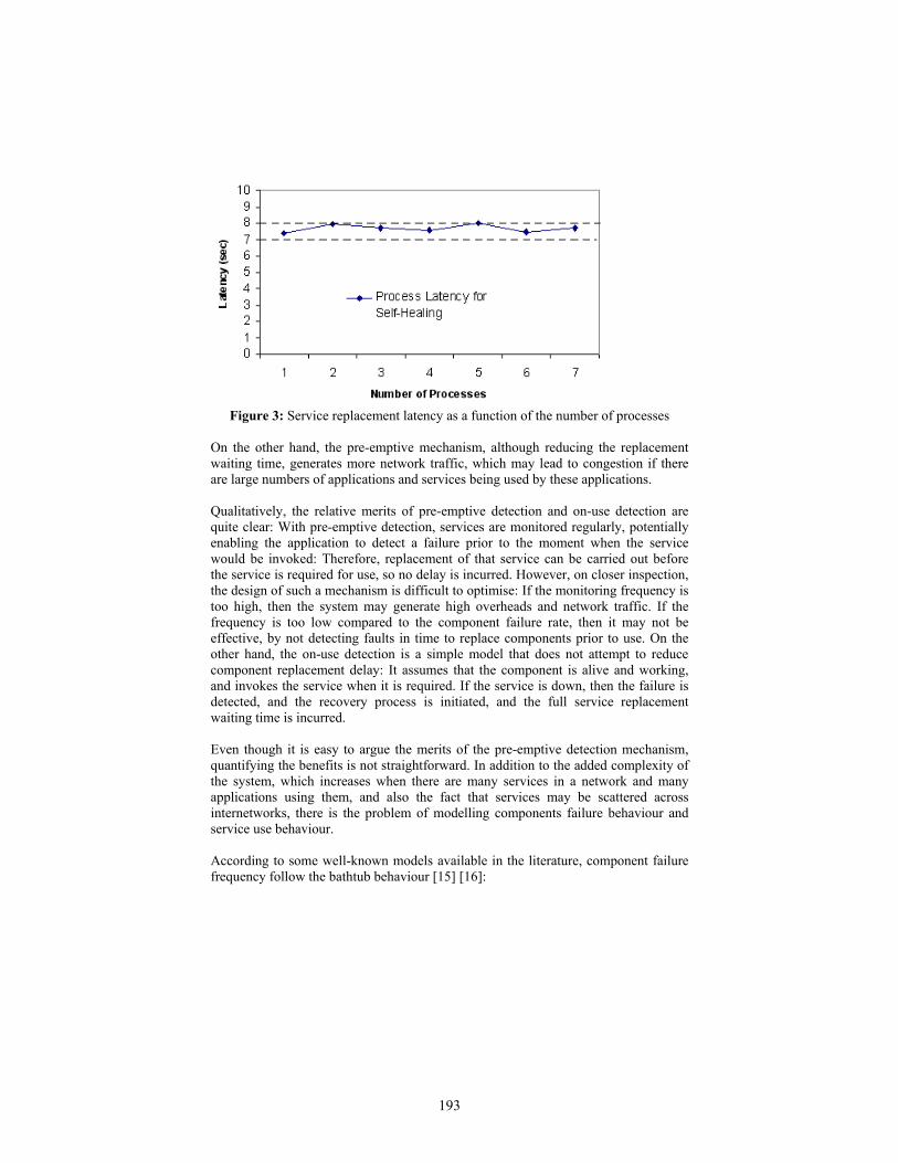
Figure 3: Service replacement latency as a function of the number of processes
On the other hand, the pre-emptive mechanism, although reducing the replacement waiting time, generates more network traffic, which may lead to congestion if there are large numbers of applications and services being used by these applications. Qualitatively, the relative merits of pre-emptive detection and on-use detection are quite clear: With pre-emptive detection, services are monitored regularly, potentially enabling the application to detect a failure prior to the moment when the service would be invoked: Therefore, replacement of that service can be carried out before the service is required for use, so no delay is incurred. However, on closer inspection, the design of such a mechanism is difficult to optimise: If the monitoring frequency is too high, then the system may generate high overheads and network traffic. If the frequency is too low compared to the component failure rate, then it may not be effective, by not detecting faults in time to replace components prior to use. On the other hand, the on-use detection is a simple model that does not attempt to reduce component replacement delay: It assumes that the component is alive and working, and invokes the service when it is required. If the service is down, then the failure is detected, and the recovery process is initiated, and the full service replacement waiting time is incurred. Even though it is easy to argue the merits of the pre-emptive detection mechanism, quantifying the benefits is not straightforward. In addition to the added complexity of the system, which increases when there are many services in a network and many applications using them, and also the fact that services may be scattered across internetworks, there is the problem of modelling components failure behaviour and service use behaviour. According to some well-known models available in the literature, component failure frequency follow the bathtub behaviour [15] [16]:
193
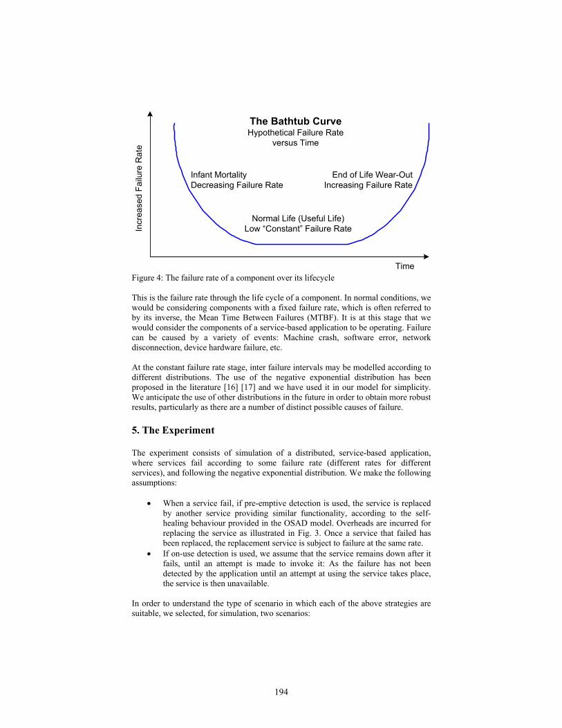
Time
Incr
ease
d Fa
ilure
Rat
e
Normal Life (Useful Life)Low “Constant” Failure Rate
Infant MortalityDecreasing Failure Rate
End of Life Wear-OutIncreasing Failure Rate
The Bathtub CurveHypothetical Failure Rate
versus Time
Figure 4: The failure rate of a component over its lifecycle This is the failure rate through the life cycle of a component. In normal conditions, we would be considering components with a fixed failure rate, which is often referred to by its inverse, the Mean Time Between Failures (MTBF). It is at this stage that we would consider the components of a service-based application to be operating. Failure can be caused by a variety of events: Machine crash, software error, network disconnection, device hardware failure, etc. At the constant failure rate stage, inter failure intervals may be modelled according to different distributions. The use of the negative exponential distribution has been proposed in the literature [16] [17] and we have used it in our model for simplicity. We anticipate the use of other distributions in the future in order to obtain more robust results, particularly as there are a number of distinct possible causes of failure. 5. The Experiment The experiment consists of simulation of a distributed, service-based application, where services fail according to some failure rate (different rates for different services), and following the negative exponential distribution. We make the following assumptions:
• When a service fail, if pre-emptive detection is used, the service is replaced by another service providing similar functionality, according to the self-healing behaviour provided in the OSAD model. Overheads are incurred for replacing the service as illustrated in Fig. 3. Once a service that failed has been replaced, the replacement service is subject to failure at the same rate.
• If on-use detection is used, we assume that the service remains down after it fails, until an attempt is made to invoke it: As the failure has not been detected by the application until an attempt at using the service takes place, the service is then unavailable.
In order to understand the type of scenario in which each of the above strategies are suitable, we selected, for simulation, two scenarios:
194

The first scenario is the scenario where an application consists of a large number of services, all of which have a fairly high failure rate. This could, for instance, represent a network of sensors and similar small devices, interconnected through a combination of unreliable wireless links and fixed networks. The second scenario represents a more stable environment where services are more reliable, having lower failure rate and being connected through a more reliable fixed network infra structure. In addition to that, for both scenarios, we assume the application invokes the services on a regular basis, for instance to monitor temperature, take a pressure reading or similar action. 5.1 First Scenario For this simulation, the following setting was adopted: Number of Services: 15 Distribution of Interfailure Interval: Negative exponential, with mean values MTBFi,:
MTBF1: 5 Mins, MTBFi+1= MTBFi+5 Mins
The simulation was allowed to run for 15 hours. Service invocation frequency: 1 invocation of each service, every 5 Mins. For the pre-emptive detection scheme, the service manager monitors each service also on a regular basis: 2 monitoring periods were chosen: 1 minute and 2.5 minutes.
195
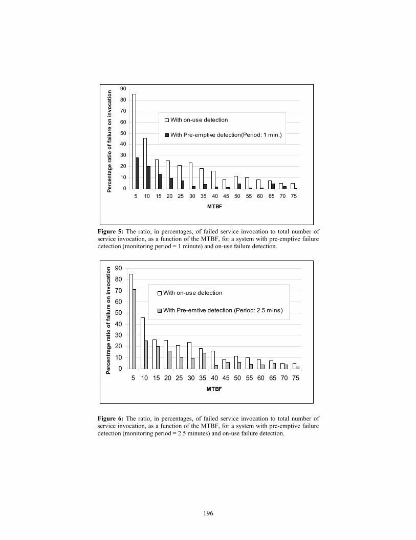
0
10
20
30
40
50
60
70
80
90
5 10 15 20 25 30 35 40 45 50 55 60 65 70 75
MTBF
Perc
enta
ge ra
tio o
f fai
lure
on
invo
catio
n
With on-use detection
With Pre-emptive detection(Period: 1 min.)
Figure 5: The ratio, in percentages, of failed service invocation to total number of service invocation, as a function of the MTBF, for a system with pre-emptive failure detection (monitoring period = 1 minute) and on-use failure detection.
0
10
20
30
40
50
60
70
80
90
5 10 15 20 25 30 35 40 45 50 55 60 65 70 75MTBF
Perc
entr
age
ratio
of f
ailu
re o
n in
voca
tion
With on-use detection
With Pre-emtive detection (Period: 2.5 mins)
Figure 6: The ratio, in percentages, of failed service invocation to total number of service invocation, as a function of the MTBF, for a system with pre-emptive failure detection (monitoring period = 2.5 minutes) and on-use failure detection.
196

The results indicate the percentage ratio of the number of times the service was down when invoked, to the total number of service invocation, with both schemes. As would be expected, for a given invocation rate, the larger the MTBF, the lower the percentage of invocations that fail. However, it is the frequency of failure monitoring, relative to the invocation frequency, which determines the percentage of failed services that are detected successfully. From figures 5 and 6, we see the obvious fact that, for a fixed invocation rate, the higher the failure rate, the higher the percentage of failed invocations. The white bars in both graphs show the same values. The black bar in figure 5 shows the percentage of failures not detected, when pre-emptive detection was used, with a period of 1 min. The grey bar in figure 6 show the percentage of failures not detected, when pre-emptive detection was used, with a period of 2.5 minutes. 5.2 Second Scenario For this simulation, the following setting was adopted: Number of Services: 1 Distribution of Interfailure Interval: Negative exponential, with mean values MTBF1,: MTBF1: 300 Mins. The application was allowed to run for 50 hours of simulated time. Service invocation frequency: every 5 Mins. As in the first scenario, the pre-emptive fault detection scheme periods use were: 1 minute and 2.5 minutes. With on use detection, the percentage of failed invocations were 1.5 %. With pre-emptive detection, with period 1 min., the percentage was 0.68% and with 2.5 minute period it was 1.2%. This reinforces the conclusions from the first scenario: With very low failure rate, compared to the service invocation rate, it is very unlikely that a service will fail in the first place, so improvement in failure detection is relatively small by using pre-emptive detection 6. Evaluation of the experiment The experiment made a number of assumptions, due to the lack of available data: Inter-failure intervals distributions were assumed to be negative exponential. This may not be a very accurate model when there are many possible, independent causes of failure. Service invocations were assumed to take place at regular intervals. This may be justifiable in some cases, such as monitoring physical values such as temperature and pressure, but is less justifiable in other types of systems.
197

However, it provides an approximated overall understanding of the issue of failure monitoring, and some guidance as to the range of usability of the different schemes proposed. 7. Conclusion This paper presents a performance discussion of the relative merits of two mechanisms for fault detection in our middleware for self-healing applications. The pre-emptive and on-use mechanisms are introduced and a discussion of their relative merits presented. It is shown that the pre-emptive mechanism reduces waiting time at the expense of higher network traffic. Future work will include the use of different failure interval distributions, and a random pattern for service invocation. References 1. J. O. Kephart, D.M.C., The Vision of Autonomic Computing. 2003, IBM
Tomas J. Watson Research Center. 2. IBM, Introduction to Autonomic Computing. 2001, IBM Corporation,
Software Group: Somers, NY. 3. Koopman, P. Elements of the Self-Healing System Problem Space. in ICSE
WADS03. 2003. Portland. 4. P. Oriezy, M.M.G., R. N. Taylor, G. Johnson, N. Medvidovic, A. Quilici, D.
Rosenblum, and A. Wolf, An Architecture-Based Approach to Self-Adaptive Software. IEEE Intellingent Systems, 1999.
5. M. Mikic-Rakic, N.M., N. Medvidovic. Architectural Style Requirements for Self-Healing Systems. in Wass'02. 2002. Charleston, South Carolina, USA.
6. E. Grishikashvili, N.B., A. Taleb-Bendiab. Service-Oriented Approach for Distributed application Assembly and Management. in The 4th Annual Postgraduate Symposium on the Convergence, Telecommunication, Networking and Broadcasting. PgNet. 2003. Liverpool, UK: LJMU.
7. Bieber, G., Openwings - Closing the Personal Digital Divide. 2001, Motorola.
8. Microsystems. Jini Network Technology. Sun Microsystems. 2000. http://wwws.sun.com/software/jini
9. Newmarch, J. Guide to Jini technology. J. Newmarch. 1999. 13 October 2004. http://jan.netcomp.monash.edu.au/java/jini/tutorial/Jini.xml
10. Badr, N. An Investigation into Autonomic Middleware Control Services to Support Distributed Self-Adaptive Software. Academic. Department, Liverpool John Moores University. 2003. Liverpool
11. D. Garlan, B.S. Model-Based Adaptation for Self-Healing Systems. in WOSS'02. 2002. Charleston, South Carolina, USA.
12. D. Reilly, A.T.-B., A. Laws, N. Badr. An Instrumentation and Control-Based Approach for Distributed Application Management and Adaptation. in Woss'02. 2002. Charleston, South Carolina, USA.
13. Gross, P.N. An Active Events Model for Systems Monitoring. in Complex and Dynamic System Architecture. 2001. Brisbane, Australia.
14. Pereira, E.G. IMPROMPTU: Software Framework for Self-Healing Middleware Services. Academic. Department, Liverpool John Moores University. 2005. Liverpool
198

15. Wilkins, D.J. The Bathtub Curve and Product Failure Behavior. Reliability Hot Wire. 2002. 11/01/2005. http://www.weibull.com/hotwire/issue21/hottopics21.htm
16. SemiconFareast. Life Distribution. Semicon Fareast. 2004. http://www.semiconfareast.com/lifedist.htm
17. Chang, Y.K., S., Computing System Failure Frequencies and Reliability Impotance Measures Using OBDD. IEEE Transactions on Computers, 2004. Vol. 53.
199