221B Lecture NotesScattering Theory II

1 Born Approximation

Lippmann–Schwinger equation

|ψ〉 = |φ〉+1

E −H0 + iεV |ψ〉, (1)

is an exact equation for the scattering problem, but it still is an equation tobe solved because the state vector |ψ〉 appears on both sides of the equation.In the coordinate space, as we derived in Scattering Theory I, it becomes

ψ(~x) ' 1

(2πh)3/2ei~k·~x − 2m

h2

eikr

4πr

∫d~x′e−i~k′·~x′

V (~x′)ψ(~x′), (2)

far away from the scatterer where r = |~x| and ~k′ = ~k~x

ris the wave-vector

of the scattered wave. Note that |~k′| = ~k. It is an integral equation for theunknown function ψ(~x).

One way to solve the Lippmann–Schwinger equation Eq. (1) is by pertur-bation theory, i.e., a power series expansion in the potential V . Note that, inthe absence of the potential, |ψ〉 = |φ〉, or in other words, |ψ〉 = |φ〉+O(V ).Therefore the lowest (1st) order approximation in V is write

|ψ〉 = |φ〉+1

E −H0 + iεV |φ〉+O(V 2), (3)

and neglect O(V 2) correction. This is called Born approximation,1 or morecorrectly, 1st Born approximation. Obviously, this approximation is goodonly when the scattering is weak.

In the coordinate space, we again replace ψ by φ in the r.h.s. of Eq. (2),and find

ψ(~x) ' 1

(2πh)3/2ei~k·~x − 2m

h2

eikr

4πr

∫d~x′e−i~k′·~x′

V (~x′)1

(2πh)3/2ei~k·~x′

=1

(2πh)3/2

[ei~k·~x − 2m

h2

eikr

4πr

∫d~x′V (~x′)ei~q·~x′

], (4)

1Did you know that Max Born was the grandfather of Olivia Newton-John? See, e.g.,http://mooni.fccj.org/~ethall/trivia/trivia.htm.

1

where ~q = ~k − ~k′ is the momentum transfer in the scattering process.The expression Eq. (4) is very interesting. It shows that the scattering

amplitude is the Fourier transform of the potential,

f (1)(~k′, ~k) = − 1

4π

2m

h2

∫d~xV (~x)ei~q·~x, (5)

up to a numerical factor of −(1/4π)(2m/h2). The superscript shows thatthis is a result valid at the first order in V . This expression demonstrates theuncertainty principle: to probe small-scale structure of an object, you needto have a scattering experiment with a high momentum transfer, because theFourier transform averages out small-scale structure otherwise.

If the potential is central, i.e., V (~x) is a function of r = |~x| only. Thenthe expression Eq. (5) can be further simplified:

f (1)(~k′, ~k) = − 1

4π

2m

h2

∫d cos θdφr2drV (r)eiqr cos θ

= −mh2

∫ ∞

0drr2V (r)

eiqr − e−iqr

iqr

= −2m

h2

1

q

∫ ∞

0drrV (r) sin qr. (6)

Therefore the scattering amplitude depends only on q = |~q| = |~k − ~k′| =

2k sin(θ/2). In other words, it is a function of the polar angle θ only f(~k′, ~k) =f(θ). This is a statement independent of Born approximation.

2 Rutherford Scattering

Rutherford is of course famous for his discovery that the atoms consist ofelectrons and a concentrated positive electric charge that we now call nuclei.He made this discovery by bombarding the α-particle on a gold foil, andlooking for events where the α-particle is scattered by a large angle. Appar-ently he suggested a poor student Marsden to do this search thinking thathe would never find one.2 Great discoveries can’t be planned.

2See, e.g., http://galileo.phys.virginia.edu/classes/252/Rutherford_Scattering/Rutherford_Scattering.html

2

2.1 Point Coulomb Source

One of the most important application of the Born approximation is to theCoulomb potential, because this is the relevant one for the Rutherford scat-tering experiment. By taking

V (r) =ZZ ′e2

r, (7)

where I took the unit where 4πε0 = 1, we would like to calculate the differ-ential cross section. Z is the charge of the scatterer (say, gold nucleus) andZ ′ that of the incident particle (say, α particle). However, the expressionEq. (6) does not converge. Therefore, we start with a short-range potentialcalled Yukawa potential

V (r) = V0e−µr

r, (8)

and take the limit µ→ 0 to recover the Coulomb potential at the end of thecalculations.3 The Yukawa potential is a typical example of a short-rangedpotential because it goes rapidly to zero once r >∼ 1/µ. It is of great intereston its own apart from the limit µ → 0. The potential that binds protonsand nucleons (nuclear force, or strong interaction) can be approximated bythis type of potential, because the range of the nuclear force is only about10−12 cm at most.

The formula Eq. (6) tells us that the scattering amplitude for the Yukawapotential Eq. (8) is

f(θ) = −2mV0

h2

1

q2 + µ2. (9)

Different cross section is therefore given by

dσ

dΩ= |f(θ)|2 =

(2mV0

h2

)2 1

[2k2(1− cos θ) + µ2]2. (10)

The total cross section is obtained by integrating over dΩ = d cos θdφ,

σ =(

2mV0

h2

)2 4π

4k2µ2 + µ4. (11)

3My normalization of V0 is different from J.J. Sakurai by a factor of µ, so that µ → 0limit is taken more easily.

3

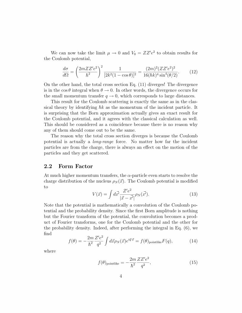
We can now take the limit µ → 0 and V0 = ZZ ′e2 to obtain results forthe Coulomb potential,

dσ

dΩ=

(2mZZ ′e2

h2

)21

[2k2(1− cos θ)]2=

(2m)2(ZZ ′e2)2

16(hk)4 sin4(θ/2). (12)

On the other hand, the total cross section Eq. (11) diverges! The divergenceis in the cos θ integral when θ → 0. In other words, the divergence occurs forthe small momentum transfer q → 0, which corresponds to large distances.

This result for the Coulomb scattering is exactly the same as in the clas-sical theory by identifying hk as the momentum of the incident particle. Itis surprising that the Born approximation actually gives an exact result forthe Coulomb potential, and it agrees with the classical calculation as well.This should be considered as a coincidence because there is no reason whyany of them should come out to be the same.

The reason why the total cross section diverges is because the Coulombpotential is actually a long-range force. No matter how far the incidentparticles are from the charge, there is always an effect on the motion of theparticles and they get scattered.

2.2 Form Factor

At much higher momentum transfers, the α-particle even starts to resolve thecharge distribution of the nucleus ρN(~x). The Coulomb potential is modifiedto

V (~x) =∫d~x′

Z ′e2

|~x− ~x′|ρN(~x′). (13)

Note that the potential is mathematically a convolution of the Coulomb po-tential and the probability density. Since the first Born amplitude is nothingbut the Fourier transform of the potential, the convolution becomes a prod-uct of Fourier transforms, one for the Coulomb potential and the other forthe probability density. Indeed, after performing the integral in Eq. (6), wefind

f(θ) = −2m

h2

Z ′e2

q2

∫d~xρN(~x)ei~q·~x = f(θ)pointlikeF (q), (14)

where

f(θ)pointlike = −2m

h2

ZZ ′e2

q2, (15)

4

F (q) =1

Z

∫d~xρN(~x)ei~q·~x. (16)

Clearly f(θ)pointlike is the scattering amplitude for the point-like Coulombsource, namely µ→ 0 limit in Eq. (9). The second factor F (q) is called theform factor which depends on the charge distribution of the nucleus. In thelimit ~q → 0, ei~q·~x = 1 and hence F (q) = 1; namely the momentum transfer istoo low to resolve the detailed structure of the nucleus. On the other hand,for large q, F (q) becomes much less than unity due to the rapidly oscillatingintegrand and the cross section gets suppressed.

The differential cross section reduces to the form

dσ

dΩ=

dσ

dΩ

∣∣∣∣∣pointlike

|F (q)|2. (17)

In fact, Rutherford experiment already showed the deviation from the point-like Coulomb source at high momentum transfer (large angle scattering),which led him to estimate the size of the nucleus.

Fig. 1 shows the form factor |F (q)|2 in an electron-nucleus scatteringexperiment. The oscillatory behavior can be understood qualitatively in thefollowing way. Imagine a sphere of radius a with a uniform charge density ρ0

such that Z = 4π3a3ρ0. The form factor, the Fourier transform, is given by

F (q) =1

Z

∫d~xρN(~x)ei~q·~x (18)

=1

Z

∫ 2π

0dφ∫ 1

−1d cos θ

∫ a

0r2drρ0e

iqr cos θ (19)

=1

Z2π∫ a

0r2drρ0

eiqr − e−iqr

iqr(20)

= 3sin aq − aq cos aq

(aq)3. (21)

One can verify that F (0) = 1. On the other hand, this function goes down as1/q2 at large q, while it oscillates in the numerator. It oscillates because theFourier transform depends sensitively on how many waves fit inside the nu-cleus. The true charge density distribution is not sharply cutoff as a uniformsphere, but somewhat smoothed out at the edge, but still similar. Fouriertransform of the measured form factor determined the true charge densitydistribution inside the nucleus, as seen in Fig. 2

5

Figure 1: Elastic electron scattering off calcium. Taken from J. B. Bellicardet al, Phys. Rev. Lett., 19, 527 (1967)

6

Figure 2: Taken from B. Hahn, D. G. Ravenhall, and R. Hofstadter, Phys.Rev. 101, 1131-1142 (1956).

7

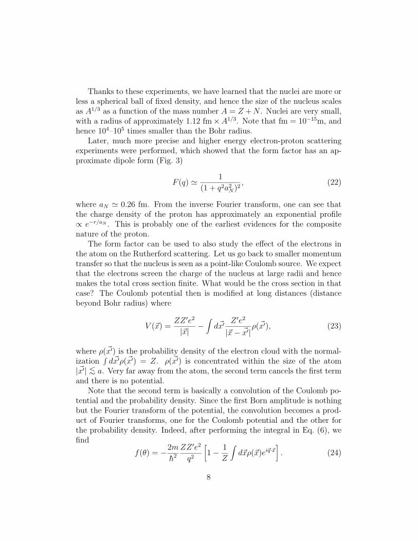
Thanks to these experiments, we have learned that the nuclei are more orless a spherical ball of fixed density, and hence the size of the nucleus scalesas A1/3 as a function of the mass number A = Z +N . Nuclei are very small,with a radius of approximately 1.12 fm×A1/3. Note that fm = 10−15m, andhence 104–105 times smaller than the Bohr radius.

Later, much more precise and higher energy electron-proton scatteringexperiments were performed, which showed that the form factor has an ap-proximate dipole form (Fig. 3)

F (q) ' 1

(1 + q2a2N)2

, (22)

where aN ' 0.26 fm. From the inverse Fourier transform, one can see thatthe charge density of the proton has approximately an exponential profile∝ e−r/aN . This is probably one of the earliest evidences for the compositenature of the proton.

The form factor can be used to also study the effect of the electrons inthe atom on the Rutherford scattering. Let us go back to smaller momentumtransfer so that the nucleus is seen as a point-like Coulomb source. We expectthat the electrons screen the charge of the nucleus at large radii and hencemakes the total cross section finite. What would be the cross section in thatcase? The Coulomb potential then is modified at long distances (distancebeyond Bohr radius) where

V (~x) =ZZ ′e2

|~x|−∫d~x′

Z ′e2

|~x− ~x′|ρ(~x′), (23)

where ρ(~x′) is the probability density of the electron cloud with the normal-ization

∫d~x′ρ(~x′) = Z. ρ(~x′) is concentrated within the size of the atom

|~x′| <∼ a. Very far away from the atom, the second term cancels the first termand there is no potential.

Note that the second term is basically a convolution of the Coulomb po-tential and the probability density. Since the first Born amplitude is nothingbut the Fourier transform of the potential, the convolution becomes a prod-uct of Fourier transforms, one for the Coulomb potential and the other forthe probability density. Indeed, after performing the integral in Eq. (6), wefind

f(θ) = −2m

h2

ZZ ′e2

q2

[1− 1

Z

∫d~xρ(~x)ei~q·~x

]. (24)

8

Figure 3: Elastic electron-proton scattering cross section compared to thedipole form factor. Taken from P.N. Kirk et al , Phys. Rev. D 8, 63 (1973).

9

In the limit ~q → 0, where the cross section diverges, two terms in the squarebracket cancel because the second term approaches unity.

To gain more insight, let us take a simple case of the hydrogen atomZ = 1. The electron wave function in the ground state is

ψ(~x) =1√4π

2a−3/2e−r/a. (25)

a = h2/me2 is the Bohr radius. The probability density of the electron cloudis then

ρ(~x) = |ψ(~x)|2 =1

πa3e−2r/a. (26)

All we need to know now is the Fourier transform of this probability density.It is straightforward to obtain∫

d~xρ(~x)ei~q·~x =16

(4 + q2a2)2. (27)

For ~q → 0, the l.h.s. is simply the normalization of the wave function, i.e.,unity. The r.h.s. indeed gives the same limit. On the other hand, it vanisheswhen q a−1. In other words, for momentum transfer larger than theinverse size of the atom h/a, the electron cloud does not change the crosssection from the case of a point Coulomb source.

Eq. (24) is now given by

f(θ) = −2m

h2 Z′e2a2 8 + 4(qa)2

(4 + (qa)2)2. (28)

When q → 0, the amplitude is regular and the total cross section converges.Recalling q2 = 2k2(1− cos θ), we find

σ =∫dΩ|f(θ)|2 = 2π

(2m

h2 Z′e2a2

)2 − (k2a2) + 2 (1 + k2a2) log(1 + k2a2)

k2a2 + k4a4

(29)For small k a−1, the last factor becomes unity, and the total cross sectionis

σ(k = 0) = 2π(

2m

h2 Z′e2a2

)2

= 8πZ ′2(m

me

)2

a2. (30)

However, this result cannot be true. The geometric cross section of thetarget (the atom) is only of the order of πa2. Because m me, this total

10

cross section is far larger than the geometric cross section. It signals thebreakdown of perturbation theory: the Born approximation is invalid. Usingthe discussion of the validity in the next section, one can also see explicitlywhy that is the case. On the other hand, for a high momentum k a−1,

σ ' 8πZ ′2(m

me

)2

a2 2 log(1 + k2a2)− 1

k2a2. (31)

As long as k a−1(m/me), Born approximation is valid and the total crosssection can be trusted.

2.3 Coulomb Wave Function

Back to the point-like Coulomb source, we obtained the Rutherford formulawith the 1st Born approximation, which agrees with purely classical result.We have also seen that the long-range nature of the Coulomb potential actu-ally results in an infinite total cross section. The long-range nature, however,causes another problem. Because the α-particle (or any charged particle forthat matter) feels the Coulomb potential no matter how far it is, the incidentwave can never be described accurately by a plane wave. In fact, there is alogarithmic correction to it. We do not go into the discussion in detail inthis lecture note, but you can look at the very last section of Sakurai on thisissue. Instead of plane waves, you are supposed to use the Coulomb wavefunctions, which are the exact solutions to the Schrodinger equation in thepresence of the Coulomb energy with positive energies (non-bound and hencecontinuum state) with a definite angular momentum.

Fortunately, the result obtained from the exact solution turns out to agreeboth with the Born approximation and the classical result. Rutherford waslucky in many ways.

3 Born Expansion

Of course, the first Born approximation is only the leading order in V . Wecan work out higher orders from Eq. (3), by iteratively insert the r.h.s. of theequation at a given order in V back into the |ψ〉. We then have the infiniteseries

|ψ〉 = |φ〉+1

E −H0 + iεV |φ〉+

1

E −H0 + iεV

1

E −H0 + iεV |φ〉

11

+1

E −H0 + iεV

1

E −H0 + iεV

1

E −H0 + iεV |φ〉+ · · · . (32)

This is called Born expansion, and the Born approximation we used is nothingbut the first term in this systematic expansion. The physical meaning of thisequation is obvious. The first term is the wave which did not get scattered.The second term is the wave that gets scattered at a point in the potentialand then propagates outwards by the 1/(E − H0 + iε) operator. In thethird term, the wave gets scattered at a point in the potential, propagatesfor a while, and gets scattered again at another point in the potential, andpropagates outwards. In the n + 1-th term, there are n times scattering ofthe wave before it propagates outwards.

More formally, an operator called T -matrix is used often in scatteringproblems. The definition is

V |ψ〉 = T |φ〉. (33)

We always take |φ〉 = |h~k〉. This seemingly weird definition is actually usefulas seen below. The scattering amplitude derived in the lecture note “Scat-tering Theory I” is

f(~k′, ~k) = −(2π)3

4π

2m

h2 〈h~k′|V |ψ〉. (34)

Using the definition of the T -matrix, we find

f(~k′, ~k) = −(2π)3

4π

2m

h2 〈h~k′|T |h~k〉. (35)

Hence, the T -matrix element has a physical interpretation of the transition(hence T ) from the initial momentum h~k to the final momentum h~k′.

Using the Lippmann–Schwinger equation Eq. (1), and multiplying theboth sides by V from left, we find

T |φ〉 = V |φ〉+ V1

E −H0 + iεT |φ〉, (36)

and hence

T = V + V1

E −H0 + iεT. (37)

In other words, a formal solution to the T -matrix is

T =1

1− V 1E−H0+iε

V. (38)

12

By Taylor expanding this operator in geometric series, we find

T = V + V1

E −H0 + iεV + V

1

E −H0 + iεV

1

E −H0 + iεV + · · · . (39)

This proves the Born expansion Eq. (32).In the coordinate space, for example, the second Born term is given by

〈~x| 1

E −H0 + iεV

1

E −H0 + iεV |φ〉

=∫d~x′d ~x′′

−2m

h2

eik|~x−~x′|

4π|~x− ~x′|V (~x′)

−2m

h2

eik|~x′− ~x′′|

4π|~x′ − ~x′′|V ( ~x′′)φ( ~x′′), (40)

where φ( ~x′′) = ei~k· ~x′′/(2πh)3/2.

4 Validity of Born Approximation

Born approximation replaces ψ by φ in Lippmann–Schwinger equation, whichis integrated together with the potential. Therefore, in order for Born ap-proximation to be good, the difference between ψ and φ must be small wherethe potential exists. The self-consistency requires that

|ψ(~x)− φ(~x)| |φ(~x)| (41)

where V (~x) is sizable, and the l.h.s. can be evaluated within Born approx-imation itself. From Lippmann–Schwinger equation (the one before takingthe limit of large r), we find∣∣∣∣∣∣2mh2

∫d~x′

eik|~x−~x′|

4π|~x− ~x′|V (~x′)ei~k·~x′

∣∣∣∣∣∣ 1. (42)

In particular, we require this condition at ~x = 0 where the potential is thestrongest presumably.

For a smooth central potential, with a magnitude of order V0 and a rangeof order a, we can qualitatively work out the validity constraint Eq. (42).

Taking ~k along the z axis, and looking at ~x ' 0 where the potential is mostimportant presumably (and relabeling ~x′ as ~x), the condition is

2m

h2

∣∣∣∣∣∫d~xeikr

4πrV (~x)eikz

∣∣∣∣∣ 1. (43)

13

When k a−1, we can ignore the phases in the integral, and it is givenroughly by

2m

h2 |V0|a2 1

2 1 (k a−1). (44)

Numerical coefficients are not to be trusted. On the other hand, whenk a−1, the phase factor oscillates rapidly and we can use stationaryphase approximation. The exponent is ikr + ikz, and it is stationary onlyalong the negative z-axis z = −r. Expanding around this point, it isikr + ikz = ik(x2 + y2)/r + O(x3, y3). The Gaussian integral over x, ythen gives a factor of πr/k, while z is integrated along the stationary phasedirection from −a to 0. Therefore, the validity condition is given roughly by

2m

h2

a

4k|V0| 1 (k a−1). (45)

On the other hand, we can estimate the total cross section in both limits.The scattering amplitude in the Born approximation Eq. (5) is

f (1)(~k′, ~k) = − 1

4π

2m

h2

∫d~xV (~x)ei~q·~x

∼ − 1

4π

2m

h2 V04π

3a3 (q a−1). (46)

For a large momentum transfer, say along the x axis, y and z integral eachgives a factor of a because of no phase variation, while x integral oscillatesrapidly and cancels mostly; it leaves only∼ 1/q contribution from non-precisecancellation. Therefore,

f (1)(~k′, ~k) ∼ − 1

4π

2m

h2 V0πa2

q(q a−1). (47)

Because the momentum transfer q is of the order of k (except the very forwardregion which we neglect from this discussion), the total cross sections areroughly

σ ∼

14π

(2mh2 V0

4π3a3)2

(k a−1)

14π

(2mh2 V0

πa2

q

)2k a−1).

(48)

It is interesting to note that, once the validity condition Eqs. (44,45) issatisfied, the total cross section is always smaller than the geometric cross

14

section 4πa2.

σ 16

9πa2 (k a−1) (49)

σ 4πa2 (k a−1). (50)

If you find a Born cross section larger than the geometric cross section, youshould be worried.

15