28 Jupyter Notebook tips, tricks andshortcuts12 Oct 2016

This post is based on a post that originally appeared on Alex Rogozhnikov’sblog, ‘Brilliantly Wrong’.

We have expanded the post and will continue to do so over time - if you havea suggestion please let us know in the comments. Thanks to Alex forgraciously letting us republish his work here.

Jupyter Notebook

Jupyter notebook, formerly known as the IPython notebook, is a flexible toolthat helps you create readable analyses, as you can keep code, images,comments, formulae and plots together.

Jupyter is quite extensible, supports many programming languages and iseasily hosted on your computer or on almost any server — you only need tohave ssh or http access. Best of all, it’s completely free.

The Jupyter interface.

Project Jupyter was born out of the IPython project as the project evolved tobecome a notebook that could support multiple languages - hence itshistorical name as the IPython notebook. The name Jupyter is an indirectacronyum of the three core languages it was designed for: JUlia, PYThon,and R and is inspired by the planet Jupiter.

When working with Python in Jupyter, the IPython kernel is used, whichgives us some handy access to IPython features from within our Jupyternotebooks (more on that later!)

We’re going to show you 28 tips and tricks to make your life working withJupyter easier.

1. Keyboard Shortcuts

As any power user knows, keyboard shortcuts will save you lots of time.Jupyter stores a list of keybord shortcuts under the menu at the top: Help >Keyboard Shortcuts. It’s worth checking this each time you update Jupyter,as more shortcuts are added all the time.

Another way to access keyboard shortcuts, and a handy way to learn them isto use the command palette: Cmd + Shift + P (or Ctrl + Shift + P onLinux and Windows). This dialog box helps you run any command by name -useful if you don’t know the keyboard shortcut for an action or if what youwant to do does not have a keyboard shortcut. The functionality is similar toSpotlight search on a Mac, and once you start using it you’ll wonder how youlived without it!

The command palette.

Some of my favorites:

Esc will take you into command mode where you can navigate aroundyour notebook with arrow keys.While in command mode:

A to insert a new cell above the current cell, B to insert a new cellbelow.M to change the current cell to Markdown, Y to change it back tocodeD + D (press the key twice) to delete the current cell

Enter will take you from command mode back into edit mode for thegiven cell.Shift = Tab will show you the Docstring (documentation) for the theobject you have just typed in a code cell - you can keep pressing thisshort cut to cycle through a few modes of documentation.Ctrl + Shift + - will split the current cell into two from where yourcursor is.Esc + F Find and replace on your code but not the outputs.Esc + O Toggle cell output.

Select Multiple Cells:Shift + J or Shift + Down selects the next sell in a downwardsdirection. You can also select sells in an upwards direction by usingShift + K or Shift + Up.Once cells are selected, you can then delete / copy / cut / paste / runthem as a batch. This is helpful when you need to move parts of anotebook.You can also use Shift + M to merge multiple cells.

2. Pretty Display of Variables

The first part of this is pretty widely known. By finishing a Jupyter cell withthe name of a variable or unassigned output of a statement, Jupyter willdisplay that variable without the need for a print statement. This is especiallyuseful when dealing with Pandas DataFrames, as the output is neatlyformatted into a table.

What is known less, is that you can alter a modify theast_note_interactivity kernel option to make jupyter do this for anyvariable or statement on it’s own line, so you can see the value of multiplestatements at once.

from IPython.core.interactiveshell import InteractiveShellInteractiveShell.ast_node_interactivity = "all"

from pydataset import dataquakes = data('quakes')quakes.head()quakes.tail()

lat long depth mag stations1 -20.42 181.62 562 4.8 41

2 -20.62 181.03 650 4.2 15

3 -26.00 184.10 42 5.4 43

4 -17.97 181.66 626 4.1 19

5 -20.42 181.96 649 4.0 11

lat long depth mag stations996 -25.93 179.54 470 4.4 22

997 -12.28 167.06 248 4.7 35

998 -20.13 184.20 244 4.5 34

999 -17.40 187.80 40 4.5 14

1000 -21.59 170.56 165 6.0 119

If you want to set this behaviour for all instances of Jupyter (Notebook andConsole), simply create a file~/.ipython/profile_default/ipython_config.py with the lines below.

c = get_config()

# Run all nodes interactivelyc.InteractiveShell.ast_node_interactivity = "all"

3. Easy links to documentation

Inside the Help menu you’ll find handy links to the online documentation forcommon libraries including NumPy, Pandas, SciPy and Matplotlib.

Don’t forget also that by prepending a library, method or variable with ?, youcan access the Docstring for quick reference on syntax.

Docstring:S.replace(old, new[, count]) -> str

Return a copy of S with all occurrences of substringold replaced by new. If the optional argument count isgiven, only the first count occurrences are replaced.Type: method_descriptor

4. Plotting in notebooks

There are many options for generating plots in your notebooks.

matplotlib (the de-facto standard), activated with %matplotlib inline -

Here’s a Dataquest Matplotlib Tutorial.%matplotlib notebook provides interactivity but can be a little slow,since rendering is done server-side.Seaborn is built over Matplotlib and makes building more attractiveplots easier. Just by importing Seaborn, your matplotlib plots are made‘prettier’ without any code modification.mpld3 provides alternative renderer (using d3) for matplotlib code.Quite nice, though incomplete.bokeh is a better option for building interactive plots.plot.ly can generate nice plots - this used to be a paid service only butwas recently open sourced.Altair is a relatively new declarative visualization library for Python. It’seasy to use and makes great looking plots, however the ability tocustomize those plots is not nearly as powerful as in Matplotlib.

The Jupyter interface.

5. IPython Magic Commands

The %matplotlib inline you saw above was an example of a IPython Magiccommand. Being based on the IPython kernel, Jupyter has access to all theMagics from the IPython kernel, and they can make your life a lot easier!

# This will list all magic commands%lsmagic

I recommend browsing the documentation for all IPython Magic commandsas you’ll no doubt find some that work for you. A few of my favorites arebelow:

6. IPython Magic - %env: Set Environment Variables

You can manage environment variables of your notebook without restartingthe jupyter server process. Some libraries (like theano) use environmentvariables to control behavior, %env is the most convenient way.

# Running %env without any arguments# lists all environment variables

# The line below sets the environment# variable OMP_NUM_THREADS%env OMP_NUM_THREADS=4

env: OMP_NUM_THREADS=4

7. IPython Magic - %run: Execute python code

%run can execute python code from .py files - this is well-documentedbehavior. Lesser known is the fact that it can also execute other jupyternotebooks, which can quite useful.

Note that using %run is not the same as importing a python module.

Available line magics:%alias %alias_magic %autocall %automagic %autosave %bookmark %cat %cd %clear %colors %config %connect_info %cp %debug %dhist %dirs %doctest_mode %ed %edit %env %gui %hist %history %killbgscripts %ldir %less %lf %lk %ll %load %load_ext %loadpy %logoff %logon %logstart %logstate %logstop %ls %lsmagic %lx %macro %magic %man %matplotlib %mkdir %more %mv %notebook %page %pastebin %pdb %pdef %pdoc %pfile %pinfo %pinfo2 %popd %pprint %precision %profile %prun %psearch %psource %pushd %pwd %pycat %pylab %qtconsole %quickref %recall %rehashx %reload_ext %rep %rerun %reset %reset_selective %rm %rmdir %run %save %sc %set_env %store %sx %system %tb %time %timeit %unalias %unload_ext %who %who_ls %whos %xdel %xmode

Available cell magics:%%! %%HTML %%SVG %%bash %%capture %%debug %%file %%html %%javascript %%js %%latex %%perl %%prun %%pypy %%python %%python2 %%python3 %%ruby %%script %%sh %%svg %%sx %%system %%time %%timeit %%writefile

Automagic is ON, % prefix IS NOT needed for line magics.

# this will execute and show the output from# all code cells of the specified notebook%run ./two-histograms.ipynb

8. IPython Magic - %load: Insert the code from an externalscript

This will replace the contents of the cell with an external script. You caneither use a file on your computer as a source, or alternatively a URL.

# Before Running%load ./hello_world.py

# After Running# %load ./hello_world.pyif __name__ == "__main__": print("Hello World!")

9. IPython Magic - %store: Pass variables between notebooks.

The %store command lets you pass variables between two differentnotebooks.

In [62]:

data = 'this is the string I want to pass to different notebook'%store datadel data # This has deleted the variable

Now, in a new notebook…

In [1]:

%store -r dataprint(data)

this is the string I want to pass to different notebook

10. IPython Magic - %who: List all variables of global scope.

The %who command without any arguments will list all variables that existingin the global scope. Passing a parameter like str will list only variables of thattype.

one = "for the money"two = "for the show"three = "to get ready now go cat go" %who str

11. IPython Magic - Timing

There are two IPython Magic commands that are useful for timing - %%timeand %timeit. These are especially handy when you have some slow code andyou’re trying to indentify where the issue is.

%%time will give you information about a single run of the code in your cell.

%%time

import timefor _ in range(1000): time.sleep(0.01)# sleep for 0.01 seconds

CPU times: user 21.5 ms, sys: 14.8 ms, total: 36.3 msWall time: 11.6 s

%%timeit uses the Python timeit module which runs a statement 100,000times (by default) and then provides the mean of the fastest three times.

In [3]:

import numpy%timeit numpy.random.normal(size=100)

12. IPython Magic - %%writefile and %pycat: Export thecontents of a cell/Show the contents of an external script

Using the %%writefile magic saves the contents of that cell to an external file.%pycat does the opposite, and shows you (in a popup) the syntax highlightedcontents of an external file.

%%writefile pythoncode.py

import numpydef append_if_not_exists(arr, x): if x not in arr: arr.append(x) def some_useless_slow_function(): arr = list() for i in range(10000): x = numpy.random.randint(0, 10000) append_if_not_exists(arr, x)

import numpydef append_if_not_exists(arr, x): if x not in arr: arr.append(x) def some_useless_slow_function(): arr = list() for i in range(10000): x = numpy.random.randint(0, 10000) append_if_not_exists(arr, x)

13. IPython Magic - %prun: Show how much time your programspent in each function.

The slowest run took 7.29 times longer than the fastest. This could mean that an intermediate result is being cached.100000 loops, best of 3: 5.5 µs per loop

Using %prun statement_name will give you an ordered table showing you thenumber of times each internal function was called within the statement, thetime each call took as well as the cumulative time of all runs of the function.

%prun some_useless_slow_function()

14. IPython Magic - Debugging with %pdb

Jupyter has own interface for The Python Debugger (pdb). This makes itpossible to go inside the function and investigate what happens there.

You can view a list of accepted commands for pdb here.

%pdb

def pick_and_take(): picked = numpy.random.randint(0, 1000) raise NotImplementedError() pick_and_take()

Automatic pdb calling has been turned ON

---------------------------------------------------------------------------NotImplementedError Traceback (most recent call last)<ipython-input-24-0f6b26649b2e> in <module>() 5 raise NotImplementedError() 6 ----> 7 pick_and_take()

<ipython-input-24-0f6b26649b2e> in pick_and_take() 3 def pick_and_take(): 4 picked = numpy.random.randint(0, 1000)----> 5 raise NotImplementedError() 6

26324 function calls in 0.556 seconds

Ordered by: internal time

ncalls tottime percall cumtime percall filename:lineno(function) 10000 0.527 0.000 0.528 0.000 <ipython-input-46-b52343f1a2d5>:2(append_if_not_exists) 10000 0.022 0.000 0.022 0.000 {method 'randint' of 'mtrand.RandomState' objects} 1 0.006 0.006 0.556 0.556 <ipython-input-46-b52343f1a2d5>:6(some_useless_slow_function) 6320 0.001 0.000 0.001 0.000 {method 'append' of 'list' objects} 1 0.000 0.000 0.556 0.556 <string>:1(<module>) 1 0.000 0.000 0.556 0.556 {built-in method exec} 1 0.000 0.000 0.000 0.000 {method 'disable' of '_lsprof.Profiler' objects}

7 pick_and_take()

NotImplementedError:

> <ipython-input-24-0f6b26649b2e>(5)pick_and_take() 3 def pick_and_take(): 4 picked = numpy.random.randint(0, 1000)----> 5 raise NotImplementedError() 6 7 pick_and_take()

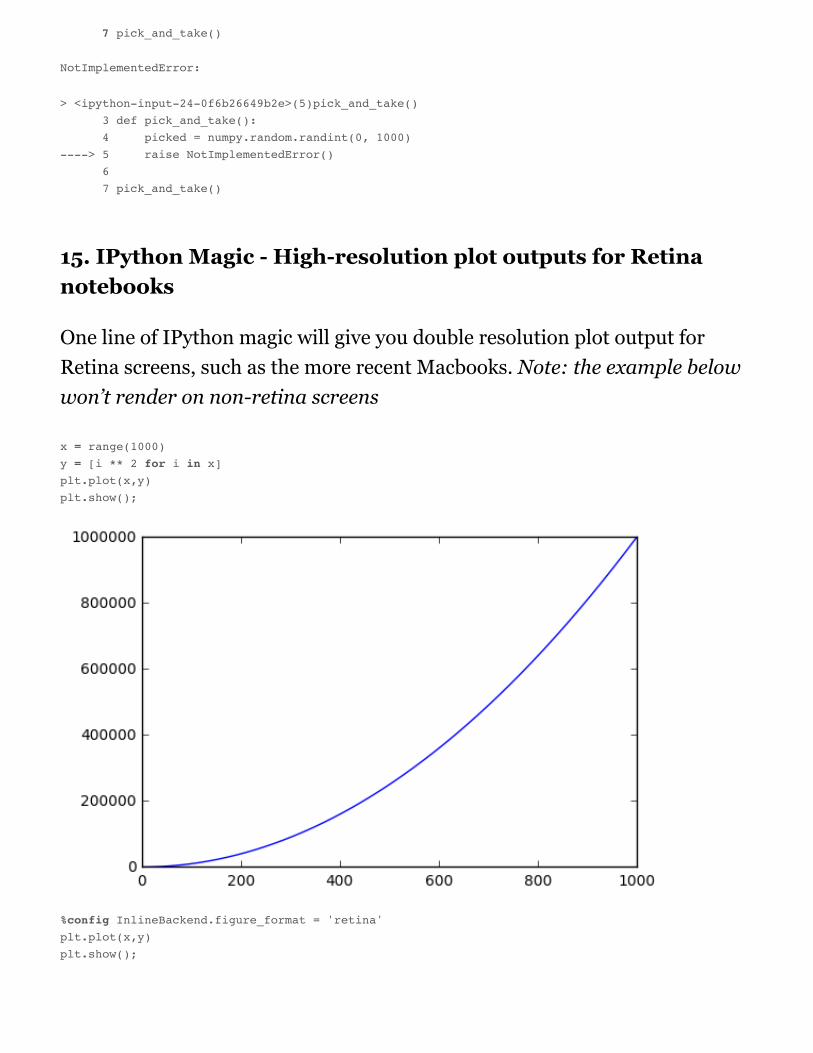
15. IPython Magic - High-resolution plot outputs for Retinanotebooks

One line of IPython magic will give you double resolution plot output forRetina screens, such as the more recent Macbooks. Note: the example belowwon’t render on non-retina screens

x = range(1000)y = [i ** 2 for i in x]plt.plot(x,y)plt.show();

%config InlineBackend.figure_format = 'retina'plt.plot(x,y)plt.show();

16. Suppress the output of a final function.

Sometimes it’s handy to suppress the output of the function on a final line, forinstance when plotting. To do this, you just add a semicolon at the end.

%matplotlib inlinefrom matplotlib import pyplot as pltimport numpyx = numpy.linspace(0, 1, 1000)**1.5

# Here you get the output of the functionplt.hist(x)

(array([ 216., 126., 106., 95., 87., 81., 77., 73., 71., 68.]), array([ 0. , 0.1, 0.2, 0.3, 0.4, 0.5, 0.6, 0.7, 0.8, 0.9, 1. ]), <a list of 10 Patch objects>)

# By adding a semicolon at the end, the output is suppressed.plt.hist(x);

17. Executing Shell Commands

It’s easy to execute a shell command from inside your notebook. You can usethis to check what datasets are in available in your working folder:

nba_2016.csv titanic.csvpixar_movies.csv whitehouse_employees.csv

Or to check and manage packages.

In [8]:

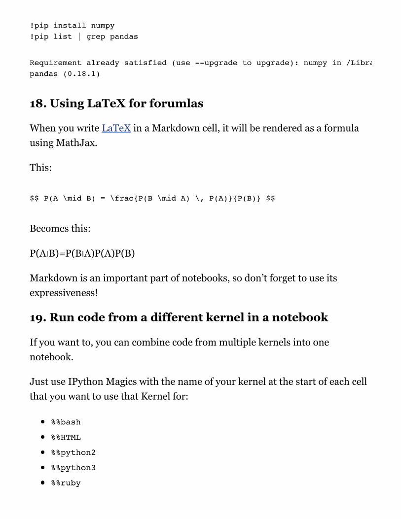
!pip install numpy!pip list | grep pandas

18. Using LaTeX for forumlas

When you write LaTeX in a Markdown cell, it will be rendered as a formulausing MathJax.

This:

$$ P(A \mid B) = \frac{P(B \mid A) \, P(A)}{P(B)} $$

Becomes this:

P(A∣B)=P(B∣A)P(A)P(B)

Markdown is an important part of notebooks, so don’t forget to use itsexpressiveness!

19. Run code from a different kernel in a notebook

If you want to, you can combine code from multiple kernels into onenotebook.

Just use IPython Magics with the name of your kernel at the start of each cellthat you want to use that Kernel for:

%%bash

%%HTML

%%python2

%%python3

%%ruby

Requirement already satisfied (use --upgrade to upgrade): numpy in /Library/Frameworks/Python.framework/Versions/3.4/lib/python3.4/site-packagespandas (0.18.1)

%%perl

%%bashfor i in {1..5}do

echo "i is $i"done

i is 1i is 2i is 3i is 4i is 5

20. Install other kernels for Jupyter

One of the nice features about Jupyter is ability to run kernels for differentlanguages. As an example, here is how to get and R kernel running.

Easy Option: Installing the R Kernel Using Anaconda

If you used Anaconda to set up your environment, getting R working isextremely easy. Just run the below in your terminal:

conda install -c r r-essentials

Less Easy Option: Installing the R Kernel Manually

If you are not using Anaconda, the process is a little more complex. Firstly,you’ll need to install R from CRAN if you haven’t already.

Once that’s done, fire up an R console and run the following:

21. Running R and Python in the same notebook.

install.packages(c('repr', 'IRdisplay', 'crayon', 'pbdZMQ', 'devtools'))devtools::install_github('IRkernel/IRkernel')IRkernel::installspec() # to register the kernel in the current R installation

The best solution to this is to install rpy2 (requires a working version of R aswell), which can be easily done with pip:

You can then use the two languages together, and even pass variablesinbetween:

array([1], dtype=int32)

import pandas as pddf = pd.DataFrame({ 'Letter': ['a', 'a', 'a', 'b', 'b', 'b', 'c', 'c', 'c'], 'X': [4, 3, 5, 2, 1, 7, 7, 5, 9], 'Y': [0, 4, 3, 6, 7, 10, 11, 9, 13], 'Z': [1, 2, 3, 1, 2, 3, 1, 2, 3] })

%%R -i dfggplot(data = df) + geom_point(aes(x = X, y= Y, color = Letter, size = Z))

Example courtesy Revolutions Blog

22. Writing functions in other languages

Sometimes the speed of numpy is not enough and I need to write some fastcode. In principle, you can compile function in the dynamic library and writepython wrappers…

But it is much better when this boring part is done for you, right?

You can write functions in cython or fortran and use those directly frompython code.

First you’ll need to install:

!pip install cython fortran-magic

%%cythondef myltiply_by_2(float x): return 2.0 * x

Personally I prefer to use fortran, which I found very convenient for writingnumber-crunching functions. More details of usage can be found here.

%%fortran

subroutine compute_fortran(x, y, z) real, intent(in) :: x(:), y(:) real, intent(out) :: z(size(x, 1))

z = sin(x + y)

end subroutine compute_fortran

compute_fortran([1, 2, 3], [4, 5, 6])

There are also different jitter systems which can speed up your python code.More examples can be found here.

23. Multicursor support

Jupyter supports mutiple cursors, similar to Sublime Text. Simply click anddrag your mouse while holding down Alt.

24. Jupyter-contrib extensions

Jupyter-contrib extensions is a family of extensions which give Jupyter a lotmore functionality, including e.g. jupyter spell-checker and code-formatter.

The following commands will install the extensions, as well as a menu basedconfigurator that will help you browse and enable the extensions from themain Jupyter notebook screen.

The nbextension configurator.

25. Create a presentation from a Jupyter notebook.

Damian Avila’s RISE allows you to create a powerpoint style presentationfrom an existing notebook.

You can install RISE using conda:

conda install -c damianavila82 rise

!pip install https://github.com/ipython-contrib/jupyter_contrib_nbextensions/tarball/master!pip install jupyter_nbextensions_configurator!jupyter contrib nbextension install --user!jupyter nbextensions_configurator enable --user

Or alternatively pip:

And then run the following code to install and enable the extension:

jupyter-nbextension install rise --py --sys-prefixjupyter-nbextension enable rise --py --sys-prefix

26. The Jupyter output system

Notebooks are displayed as HTML and the cell output can be HTML, so youcan return virtually anything: video/audio/images.

In this example I scan the folder with images in my repository and showthumbnails of the first 5:

import osfrom IPython.display import display, Imagenames = [f for f in os.listdir('../images/ml_demonstrations/') if f.endswith('.png')]for name in names[:5]: display(Image('../images/ml_demonstrations/' + name, width=100))

We can create the same list with a bash command, because magics and bashcalls return python variables:

names = !ls ../images/ml_demonstrations/*.pngnames[:5]

['../images/ml_demonstrations/colah_embeddings.png', '../images/ml_demonstrations/convnetjs.png', '../images/ml_demonstrations/decision_tree.png', '../images/ml_demonstrations/decision_tree_in_course.png', '../images/ml_demonstrations/dream_mnist.png']

27. ‘Big data’ analysis

A number of solutions are available for querying/processing large datasamples:

ipyparallel (formerly ipython cluster) is a good option for simple map-reduce operations in python. We use it in rep to train many machine

learning models in parallelpysparkspark-sql magic %%sql

28. Sharing notebooks

The easiest way to share your notebook is simply using the notebook file(.ipynb), but for those who don’t use Jupyter, you have a few options:

Convert notebooks to html file using the File > Download as > HTMLMenu option.Share your notebook file with gists or on github, both of which renderthe notebooks. See this example.

If you upload your notebook to a github repository, you can use thehandy mybinder service to allow someone half an hour ofinteractive Jupyter access to your repository.

Setup your own system with jupyterhub, this is very handy when youorganize mini-course or workshop and don’t have time to care aboutstudents machines.Store your notebook e.g. in dropbox and put the link to nbviewer.nbviewer will render the notebook from whichever source you host it.Use the File > Download as > PDF menu to save your notebook as aPDF. If you’re going this route, I highly recommend reading JuliusSchulz’s excellent article Making publication ready Python notebooks.Create a blog using Pelican from your Jupyter notebooks.

What are your favorites?

Let me know in the comments what your favorite Jupyter notebook tips are.

I also recommend the links below for further reading:

IPython built-in magicsNice interactive presentation about jupyter by Ben Zaitlen

Advanced notebooks part 1: magics and part 2: widgetsProfiling in python with jupyter4 ways to extend notebooksIPython notebook tricksJupyter vs Zeppelin for big dataMaking publication ready Python notebooks.

Josh Devlin

Marketing Lead at Dataquest.io (Learn Data Science in your Browser).Loves Data and Aussie Rules Football. Australian living in Texas.Get in touch @jaypeedevlin.