28 machine learning unsupervised hierarchical clustering
TRANSCRIPT
Machine Learning for Data MiningHierarchical Clustering
Andres Mendez-Vazquez
July 27, 2015
1 / 46
Images/cinvestav-1.jpg
Outline1 Hierarchical Clustering
DefinitionBasic Ideas
2 Agglomerative AlgorithmsIntroductionProblems with Agglomerative AlgorithmsTwo Categories of Agglomerative Algorithms
Matrix Based AlgorithmsGraph Based Algorithms
3 Divisive AlgorithmsIntroduction
4 Algorithms for Large Data SetsIntroduction
Clustering Using REpresentatives (CURE)
2 / 46
Images/cinvestav-1.jpg
Outline1 Hierarchical Clustering
DefinitionBasic Ideas
2 Agglomerative AlgorithmsIntroductionProblems with Agglomerative AlgorithmsTwo Categories of Agglomerative Algorithms
Matrix Based AlgorithmsGraph Based Algorithms
3 Divisive AlgorithmsIntroduction
4 Algorithms for Large Data SetsIntroduction
Clustering Using REpresentatives (CURE)
3 / 46
Images/cinvestav-1.jpg
Concepts
Hierarchical Clustering AlgorithmsThey are quite different from the previous clustering algorithms.
ActuallyThey produce a hierarchy of clusterings.
4 / 46
Images/cinvestav-1.jpg
Concepts
Hierarchical Clustering AlgorithmsThey are quite different from the previous clustering algorithms.
ActuallyThey produce a hierarchy of clusterings.
4 / 46
Images/cinvestav-1.jpg
Dendrogram: Hierarchical Clustering
Hierarchical ClusteringThe clustering is obtained by cutting the dendrogram at a desired level:
Each connected component forms a cluster.
5 / 46
Images/cinvestav-1.jpg
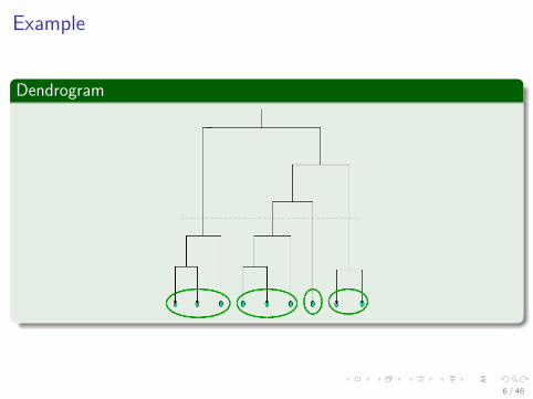
Example
Dendrogram
6 / 46
Images/cinvestav-1.jpg
Outline1 Hierarchical Clustering
DefinitionBasic Ideas
2 Agglomerative AlgorithmsIntroductionProblems with Agglomerative AlgorithmsTwo Categories of Agglomerative Algorithms
Matrix Based AlgorithmsGraph Based Algorithms
3 Divisive AlgorithmsIntroduction
4 Algorithms for Large Data SetsIntroduction
Clustering Using REpresentatives (CURE)
7 / 46
Images/cinvestav-1.jpg
Basic Ideas
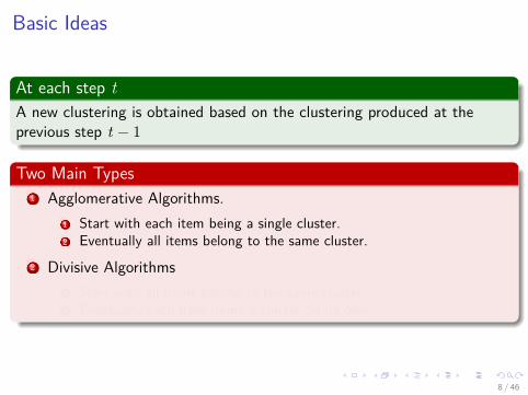
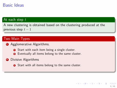
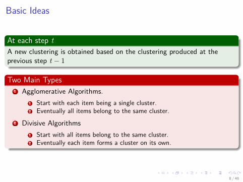
At each step tA new clustering is obtained based on the clustering produced at theprevious step t − 1
Two Main Types1 Agglomerative Algorithms.
1 Start with each item being a single cluster.2 Eventually all items belong to the same cluster.
2 Divisive Algorithms1 Start with all items belong to the same cluster.2 Eventually each item forms a cluster on its own.
8 / 46
Images/cinvestav-1.jpg
Basic Ideas
At each step tA new clustering is obtained based on the clustering produced at theprevious step t − 1
Two Main Types1 Agglomerative Algorithms.
1 Start with each item being a single cluster.2 Eventually all items belong to the same cluster.
2 Divisive Algorithms1 Start with all items belong to the same cluster.2 Eventually each item forms a cluster on its own.
8 / 46

Images/cinvestav-1.jpg
Therefore
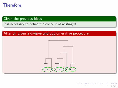
Given the previous ideasIt is necessary to define the concept of nesting!!!
After all given a divisive and agglomerative procedure
9 / 46
Images/cinvestav-1.jpg
Therefore
Given the previous ideasIt is necessary to define the concept of nesting!!!
After all given a divisive and agglomerative procedure
9 / 46
Images/cinvestav-1.jpg
Nested Clustering
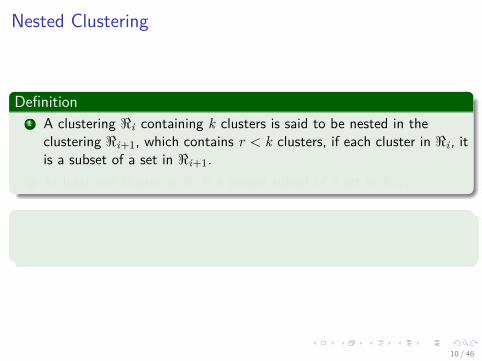
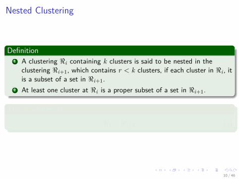
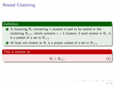
Definition1 A clustering <i containing k clusters is said to be nested in the
clustering <i+1, which contains r < k clusters, if each cluster in <i , itis a subset of a set in <i+1.
2 At least one cluster at <i is a proper subset of a set in <i+1.
This is written as
<i @ <i+1 (1)
10 / 46
Images/cinvestav-1.jpg
Nested Clustering
Definition1 A clustering <i containing k clusters is said to be nested in the
clustering <i+1, which contains r < k clusters, if each cluster in <i , itis a subset of a set in <i+1.
2 At least one cluster at <i is a proper subset of a set in <i+1.
This is written as
<i @ <i+1 (1)
10 / 46
Images/cinvestav-1.jpg
Example
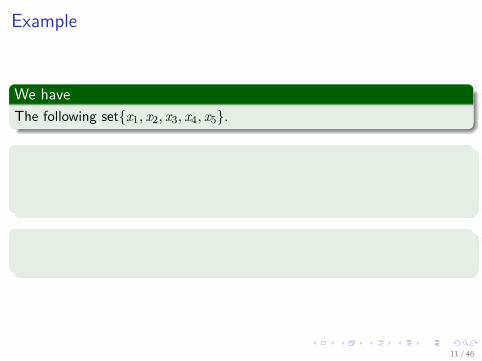
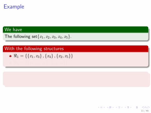
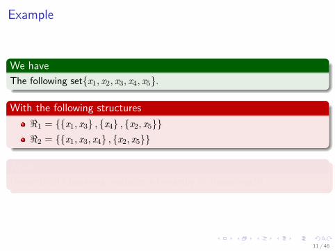
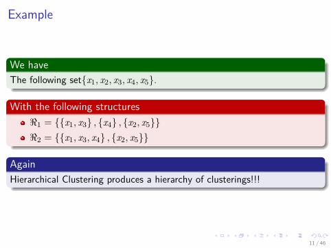
We haveThe following set{x1, x2, x3, x4, x5}.
With the following structures<1 = {{x1, x3} , {x4} , {x2, x5}}<2 = {{x1, x3, x4} , {x2, x5}}
AgainHierarchical Clustering produces a hierarchy of clusterings!!!
11 / 46
Images/cinvestav-1.jpg
Example
We haveThe following set{x1, x2, x3, x4, x5}.
With the following structures<1 = {{x1, x3} , {x4} , {x2, x5}}<2 = {{x1, x3, x4} , {x2, x5}}
AgainHierarchical Clustering produces a hierarchy of clusterings!!!
11 / 46
Images/cinvestav-1.jpg
Example
We haveThe following set{x1, x2, x3, x4, x5}.
With the following structures<1 = {{x1, x3} , {x4} , {x2, x5}}<2 = {{x1, x3, x4} , {x2, x5}}
AgainHierarchical Clustering produces a hierarchy of clusterings!!!
11 / 46
Images/cinvestav-1.jpg
Example
We haveThe following set{x1, x2, x3, x4, x5}.
With the following structures<1 = {{x1, x3} , {x4} , {x2, x5}}<2 = {{x1, x3, x4} , {x2, x5}}
AgainHierarchical Clustering produces a hierarchy of clusterings!!!
11 / 46
Images/cinvestav-1.jpg
Outline1 Hierarchical Clustering
DefinitionBasic Ideas
2 Agglomerative AlgorithmsIntroductionProblems with Agglomerative AlgorithmsTwo Categories of Agglomerative Algorithms
Matrix Based AlgorithmsGraph Based Algorithms
3 Divisive AlgorithmsIntroduction
4 Algorithms for Large Data SetsIntroduction
Clustering Using REpresentatives (CURE)
12 / 46
Images/cinvestav-1.jpg
Agglomerative Algorithms.
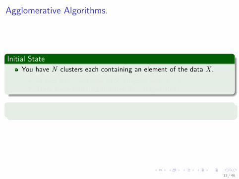
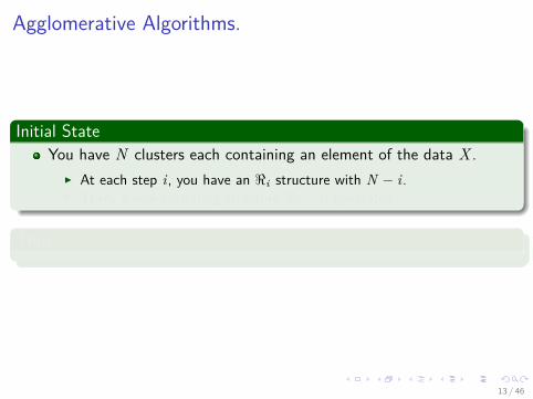
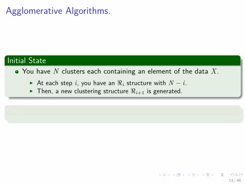
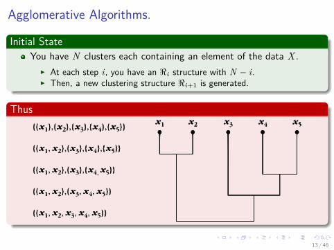
Initial StateYou have N clusters each containing an element of the data X .
I At each step i, you have an <i structure with N − i.I Then, a new clustering structure <i+1 is generated.
Thus
13 / 46
Images/cinvestav-1.jpg
Agglomerative Algorithms.
Initial StateYou have N clusters each containing an element of the data X .
I At each step i, you have an <i structure with N − i.I Then, a new clustering structure <i+1 is generated.
Thus
13 / 46
Images/cinvestav-1.jpg
Agglomerative Algorithms.
Initial StateYou have N clusters each containing an element of the data X .
I At each step i, you have an <i structure with N − i.I Then, a new clustering structure <i+1 is generated.
Thus
13 / 46
Images/cinvestav-1.jpg
Agglomerative Algorithms.
Initial StateYou have N clusters each containing an element of the data X .
I At each step i, you have an <i structure with N − i.I Then, a new clustering structure <i+1 is generated.
Thus
13 / 46
Images/cinvestav-1.jpg
In that way...
We haveAt each step, we have that each cluster <i is a proper subset of a cluste in<i or
<i @ <i+1 (2)
14 / 46
Images/cinvestav-1.jpg
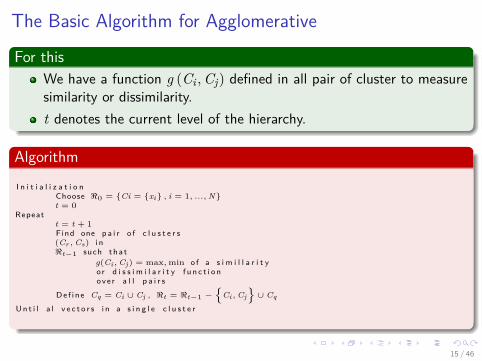
The Basic Algorithm for Agglomerative
For thisWe have a function g (Ci ,Cj) defined in all pair of cluster to measuresimilarity or dissimilarity.t denotes the current level of the hierarchy.
AlgorithmI n i t i a l i z a t i o n
Choose <0 = {Ci = {xi} , i = 1, ..., N}t = 0
Repeatt = t + 1Find one p a i r o f c l u s t e r s(Cr , Cs) i n<t−1 such t h a t
g(Ci , Cj) = max, min o f a s i m i l l a r i t yo r d i s s i m i l a r i t y f u n c t i o nove r a l l p a i r s
D e f i n e Cq = Ci ∪ Cj , <t = <t−1 −{
Ci , Cj}∪ Cq
U n t i l a l v e c t o r s i n a s i n g l e c l u s t e r
15 / 46
Images/cinvestav-1.jpg
Enforcing Nesting
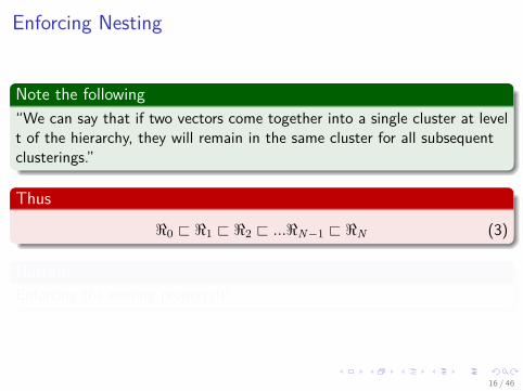
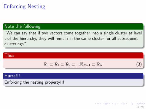
Note the following“We can say that if two vectors come together into a single cluster at levelt of the hierarchy, they will remain in the same cluster for all subsequentclusterings.”
Thus
<0 @ <1 @ <2 @ ...<N−1 @ <N (3)
Hurra!!!Enforcing the nesting property!!!
16 / 46
Images/cinvestav-1.jpg
Enforcing Nesting
Note the following“We can say that if two vectors come together into a single cluster at levelt of the hierarchy, they will remain in the same cluster for all subsequentclusterings.”
Thus
<0 @ <1 @ <2 @ ...<N−1 @ <N (3)
Hurra!!!Enforcing the nesting property!!!
16 / 46
Images/cinvestav-1.jpg
Outline1 Hierarchical Clustering
DefinitionBasic Ideas
2 Agglomerative AlgorithmsIntroductionProblems with Agglomerative AlgorithmsTwo Categories of Agglomerative Algorithms
Matrix Based AlgorithmsGraph Based Algorithms
3 Divisive AlgorithmsIntroduction
4 Algorithms for Large Data SetsIntroduction
Clustering Using REpresentatives (CURE)
17 / 46
Images/cinvestav-1.jpg
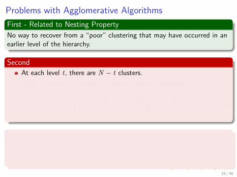
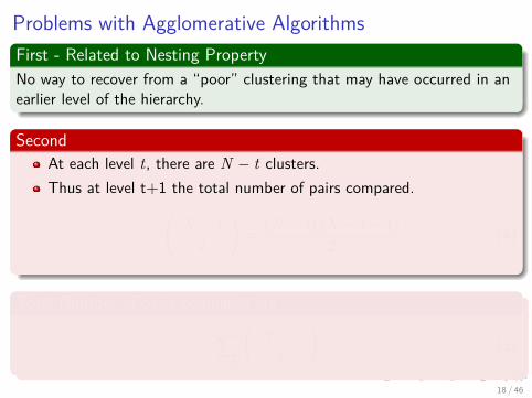
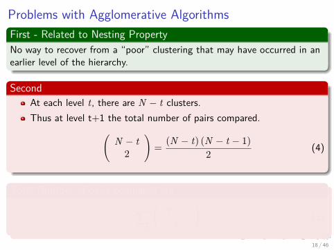
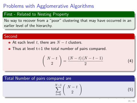
Problems with Agglomerative AlgorithmsFirst - Related to Nesting PropertyNo way to recover from a “poor” clustering that may have occurred in anearlier level of the hierarchy.
SecondAt each level t, there are N − t clusters.Thus at level t+1 the total number of pairs compared.(
N − t2
)= (N − t) (N − t − 1)
2 (4)
Total Number of pairs compared areN−1∑t=0
(N − t
2
)(5)
18 / 46
Images/cinvestav-1.jpg
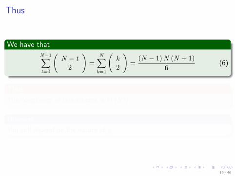
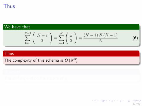
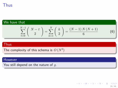
Thus
We have thatN−1∑t=0
(N − t
2
)=
N∑k=1
(k2
)= (N − 1) N (N + 1)
6 (6)
ThusThe complexity of this schema is O
(N 3)
HoweverYou still depend on the nature of g.
19 / 46
Images/cinvestav-1.jpg
Thus
We have thatN−1∑t=0
(N − t
2
)=
N∑k=1
(k2
)= (N − 1) N (N + 1)
6 (6)
ThusThe complexity of this schema is O
(N 3)
HoweverYou still depend on the nature of g.
19 / 46
Images/cinvestav-1.jpg
Thus
We have thatN−1∑t=0
(N − t
2
)=
N∑k=1
(k2
)= (N − 1) N (N + 1)
6 (6)
ThusThe complexity of this schema is O
(N 3)
HoweverYou still depend on the nature of g.
19 / 46
Images/cinvestav-1.jpg
Outline1 Hierarchical Clustering
DefinitionBasic Ideas
2 Agglomerative AlgorithmsIntroductionProblems with Agglomerative AlgorithmsTwo Categories of Agglomerative Algorithms
Matrix Based AlgorithmsGraph Based Algorithms
3 Divisive AlgorithmsIntroduction
4 Algorithms for Large Data SetsIntroduction
Clustering Using REpresentatives (CURE)
20 / 46
Images/cinvestav-1.jpg
Two Categories of Agglomerative Algorithms
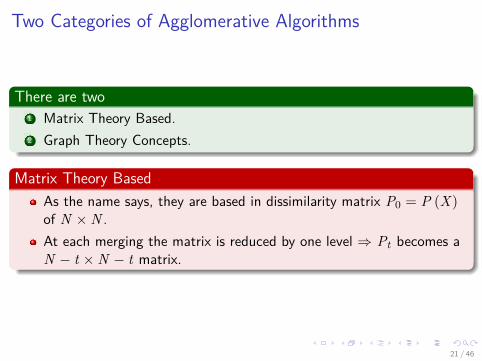
There are two1 Matrix Theory Based.2 Graph Theory Concepts.
Matrix Theory BasedAs the name says, they are based in dissimilarity matrix P0 = P (X)of N ×N .At each merging the matrix is reduced by one level ⇒ Pt becomes aN − t ×N − t matrix.
21 / 46
Images/cinvestav-1.jpg
Two Categories of Agglomerative Algorithms
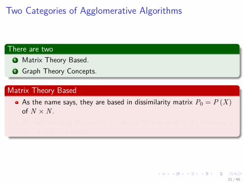
There are two1 Matrix Theory Based.2 Graph Theory Concepts.
Matrix Theory BasedAs the name says, they are based in dissimilarity matrix P0 = P (X)of N ×N .At each merging the matrix is reduced by one level ⇒ Pt becomes aN − t ×N − t matrix.
21 / 46
Images/cinvestav-1.jpg
Two Categories of Agglomerative Algorithms
There are two1 Matrix Theory Based.2 Graph Theory Concepts.
Matrix Theory BasedAs the name says, they are based in dissimilarity matrix P0 = P (X)of N ×N .At each merging the matrix is reduced by one level ⇒ Pt becomes aN − t ×N − t matrix.
21 / 46
Images/cinvestav-1.jpg
Matrix Based Algorithm
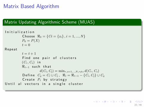
Matrix Updating Algorithmic Scheme (MUAS)
I n i t i a l i z a t i o nChoose <0 = {Ci = {xi} , i = 1, ..., N}P0 = P(X)t = 0
Repeatt = t + 1Find one p a i r o f c l u s t e r s(Cr , Cs) i n<t−1 such tha t
d(Ci , Cj) = minr,s=1,..,N,r 6=s d(Cr , Cs)Def i n e Cq = Ci ∪ Cj , <t = <t−1 − {Ci , Cj} ∪ CqCrea te Pt by s t r a t e g y
U n t i l a l v e c t o r s i n a s i n g l e c l u s t e r
22 / 46
Images/cinvestav-1.jpg
Matrix Based Algorithm
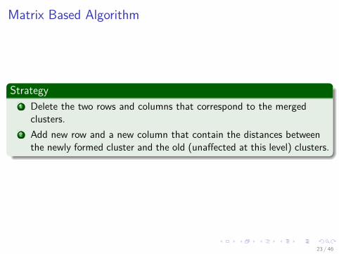
Strategy1 Delete the two rows and columns that correspond to the merged
clusters.2 Add new row and a new column that contain the distances between
the newly formed cluster and the old (unaffected at this level) clusters.
23 / 46
Images/cinvestav-1.jpg
Matrix Based Algorithm
Strategy1 Delete the two rows and columns that correspond to the merged
clusters.2 Add new row and a new column that contain the distances between
the newly formed cluster and the old (unaffected at this level) clusters.
23 / 46
Images/cinvestav-1.jpg
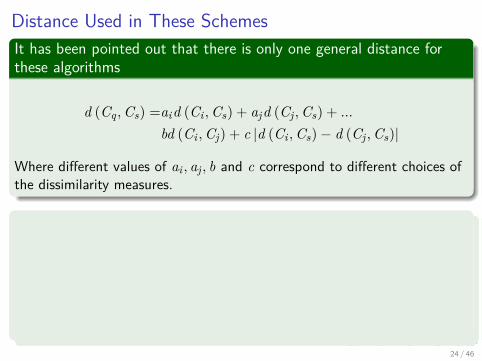
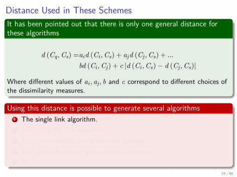
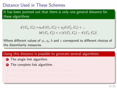
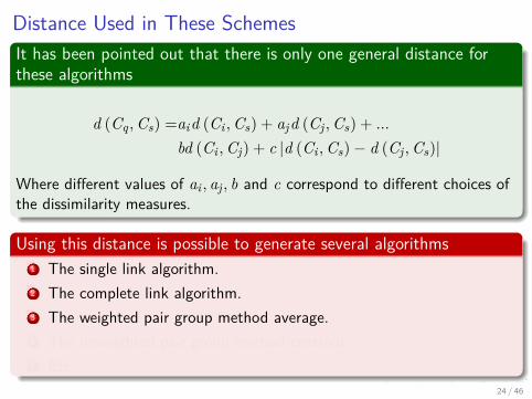
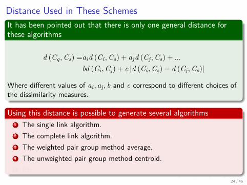
Distance Used in These SchemesIt has been pointed out that there is only one general distance forthese algorithms
d (Cq ,Cs) =aid (Ci ,Cs) + ajd (Cj ,Cs) + ...
bd (Ci ,Cj) + c |d (Ci ,Cs)− d (Cj ,Cs)|
Where different values of ai , aj , b and c correspond to different choices ofthe dissimilarity measures.
Using this distance is possible to generate several algorithms1 The single link algorithm.2 The complete link algorithm.3 The weighted pair group method average.4 The unweighted pair group method centroid.5 Etc...
24 / 46
Images/cinvestav-1.jpg
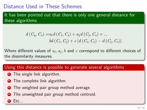
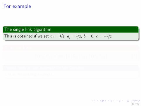
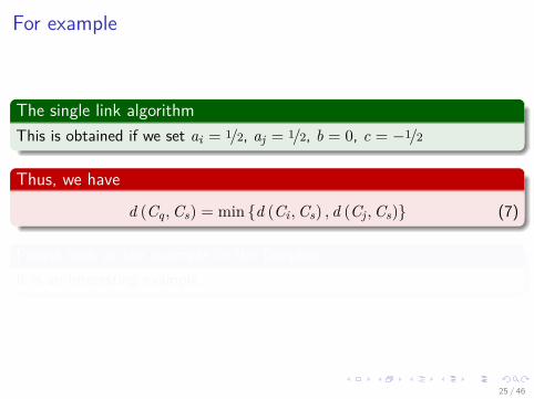
For example
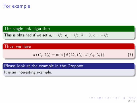
The single link algorithmThis is obtained if we set ai = 1/2, aj = 1/2, b = 0, c = −1/2
Thus, we have
d (Cq ,Cs) = min {d (Ci ,Cs) , d (Cj ,Cs)} (7)
Please look at the example in the DropboxIt is an interesting example.
25 / 46
Images/cinvestav-1.jpg
For example
The single link algorithmThis is obtained if we set ai = 1/2, aj = 1/2, b = 0, c = −1/2
Thus, we have
d (Cq ,Cs) = min {d (Ci ,Cs) , d (Cj ,Cs)} (7)
Please look at the example in the DropboxIt is an interesting example.
25 / 46
Images/cinvestav-1.jpg
For example
The single link algorithmThis is obtained if we set ai = 1/2, aj = 1/2, b = 0, c = −1/2
Thus, we have
d (Cq ,Cs) = min {d (Ci ,Cs) , d (Cj ,Cs)} (7)
Please look at the example in the DropboxIt is an interesting example.
25 / 46
Images/cinvestav-1.jpg
Agglomerative Algorithms Based on Graph Theory
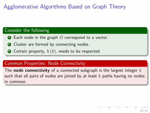
Consider the following1 Each node in the graph G correspond to a vector.2 Cluster are formed by connecting nodes.3 Certain property, h (k), needs to be respected.
Common Properties: Node ConnectivityThe node connectivity of a connected subgraph is the largest integer ksuch that all pairs of nodes are joined by at least k paths having no nodesin common.
26 / 46
Images/cinvestav-1.jpg
Agglomerative Algorithms Based on Graph Theory
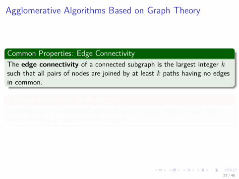
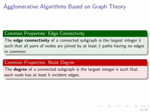
Common Properties: Edge ConnectivityThe edge connectivity of a connected subgraph is the largest integer ksuch that all pairs of nodes are joined by at least k paths having no edgesin common.
Common Properties: Node DegreeThe degree of a connected subgraph is the largest integer k such thateach node has at least k incident edges.
27 / 46
Images/cinvestav-1.jpg
Agglomerative Algorithms Based on Graph Theory
Common Properties: Edge ConnectivityThe edge connectivity of a connected subgraph is the largest integer ksuch that all pairs of nodes are joined by at least k paths having no edgesin common.
Common Properties: Node DegreeThe degree of a connected subgraph is the largest integer k such thateach node has at least k incident edges.
27 / 46
Images/cinvestav-1.jpg
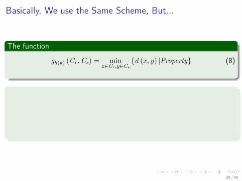
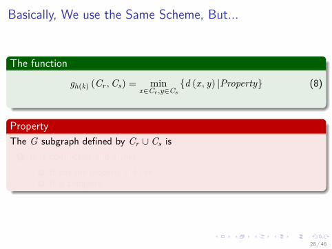
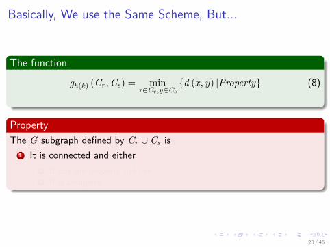
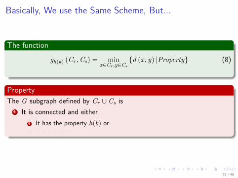
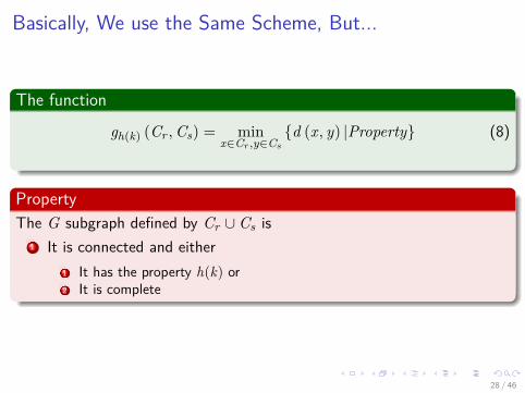
Basically, We use the Same Scheme, But...
The function
gh(k) (Cr ,Cs) = minx∈Cr ,y∈Cs
{d (x, y) |Property} (8)
PropertyThe G subgraph defined by Cr ∪ Cs is
1 It is connected and either1 It has the property h(k) or2 It is complete
28 / 46
Images/cinvestav-1.jpg
Basically, We use the Same Scheme, But...
The function
gh(k) (Cr ,Cs) = minx∈Cr ,y∈Cs
{d (x, y) |Property} (8)
PropertyThe G subgraph defined by Cr ∪ Cs is
1 It is connected and either1 It has the property h(k) or2 It is complete
28 / 46
Images/cinvestav-1.jpg
Basically, We use the Same Scheme, But...
The function
gh(k) (Cr ,Cs) = minx∈Cr ,y∈Cs
{d (x, y) |Property} (8)
PropertyThe G subgraph defined by Cr ∪ Cs is
1 It is connected and either1 It has the property h(k) or2 It is complete
28 / 46
Images/cinvestav-1.jpg
Basically, We use the Same Scheme, But...
The function
gh(k) (Cr ,Cs) = minx∈Cr ,y∈Cs
{d (x, y) |Property} (8)
PropertyThe G subgraph defined by Cr ∪ Cs is
1 It is connected and either1 It has the property h(k) or2 It is complete
28 / 46
Images/cinvestav-1.jpg
Basically, We use the Same Scheme, But...
The function
gh(k) (Cr ,Cs) = minx∈Cr ,y∈Cs
{d (x, y) |Property} (8)
PropertyThe G subgraph defined by Cr ∪ Cs is
1 It is connected and either1 It has the property h(k) or2 It is complete
28 / 46
Images/cinvestav-1.jpg
Examples
Examples1 Single Link Algorithm2 Complete Link Algorithm
There is other style of clusteringClustering Algorithms Based on the Minimum Spanning Tree
29 / 46
Images/cinvestav-1.jpg
Examples
Examples1 Single Link Algorithm2 Complete Link Algorithm
There is other style of clusteringClustering Algorithms Based on the Minimum Spanning Tree
29 / 46
Images/cinvestav-1.jpg
Examples
Examples1 Single Link Algorithm2 Complete Link Algorithm
There is other style of clusteringClustering Algorithms Based on the Minimum Spanning Tree
29 / 46
Images/cinvestav-1.jpg
Outline1 Hierarchical Clustering
DefinitionBasic Ideas
2 Agglomerative AlgorithmsIntroductionProblems with Agglomerative AlgorithmsTwo Categories of Agglomerative Algorithms
Matrix Based AlgorithmsGraph Based Algorithms
3 Divisive AlgorithmsIntroduction
4 Algorithms for Large Data SetsIntroduction
Clustering Using REpresentatives (CURE)
30 / 46
Images/cinvestav-1.jpg
Divisive Algorithms
Reverse StrategyStart with a single cluster split it iteratively.
31 / 46
Images/cinvestav-1.jpg
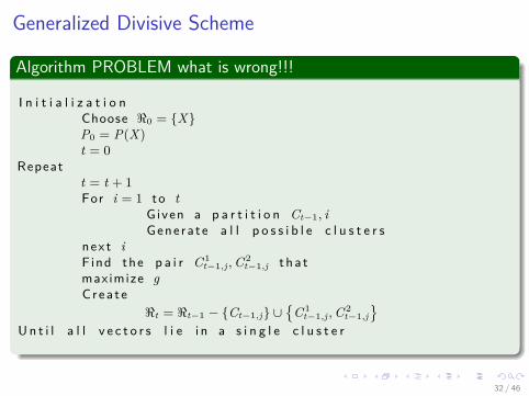
Generalized Divisive Scheme
Algorithm PROBLEM what is wrong!!!
I n i t i a l i z a t i o nChoose <0 = {X}P0 = P(X)t = 0
Repeatt = t + 1For i = 1 to t
Given a p a r t i t i o n Ct−1, iGenera te a l l p o s s i b l e c l u s t e r s
nex t iFind the p a i r C 1
t−1,j , C 2t−1,j t ha t
maximize gCrea te
<t = <t−1 − {Ct−1,j} ∪{
C 1t−1,j , C 2
t−1,j}
U n t i l a l l v e c t o r s l i e i n a s i n g l e c l u s t e r
32 / 46
Images/cinvestav-1.jpg
Outline1 Hierarchical Clustering
DefinitionBasic Ideas
2 Agglomerative AlgorithmsIntroductionProblems with Agglomerative AlgorithmsTwo Categories of Agglomerative Algorithms
Matrix Based AlgorithmsGraph Based Algorithms
3 Divisive AlgorithmsIntroduction
4 Algorithms for Large Data SetsIntroduction
Clustering Using REpresentatives (CURE)
33 / 46
Images/cinvestav-1.jpg
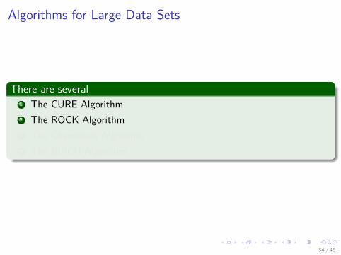
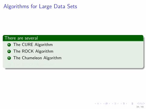
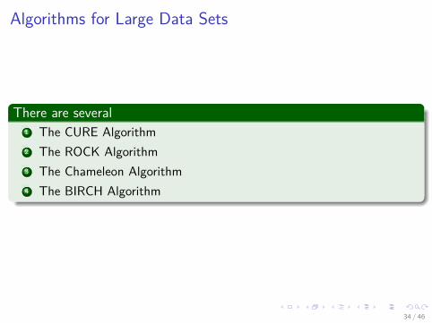
Algorithms for Large Data Sets
There are several1 The CURE Algorithm2 The ROCK Algorithm3 The Chameleon Algorithm4 The BIRCH Algorithm
34 / 46
Images/cinvestav-1.jpg
Algorithms for Large Data Sets
There are several1 The CURE Algorithm2 The ROCK Algorithm3 The Chameleon Algorithm4 The BIRCH Algorithm
34 / 46
Images/cinvestav-1.jpg
Algorithms for Large Data Sets
There are several1 The CURE Algorithm2 The ROCK Algorithm3 The Chameleon Algorithm4 The BIRCH Algorithm
34 / 46
Images/cinvestav-1.jpg
Algorithms for Large Data Sets
There are several1 The CURE Algorithm2 The ROCK Algorithm3 The Chameleon Algorithm4 The BIRCH Algorithm
34 / 46
Images/cinvestav-1.jpg
Clustering Using REpresentatives (CURE)
Basic IdeaEach cluster Ci has a set of representatives RCi =
{x(i)
1 ,x(i)2 , ...,x(i)
K
}with K > 1.
What is happeningBy using multiple representatives for each cluster, the CURE algorithmtries to “capture” the shape of each one.
HoweverIn order to avoid taking into account irregularities (For example, outliers)in the border of the cluster.
The initially chosen representatives are “pushed” toward the mean ofthe cluster.
35 / 46
Images/cinvestav-1.jpg
Therfore
This action is knownAs “Shrinking” in the sense that the volume of space “defined” by therepresentatives is shrunk toward the mean of the cluster.
36 / 46
Images/cinvestav-1.jpg
Shrinking Process
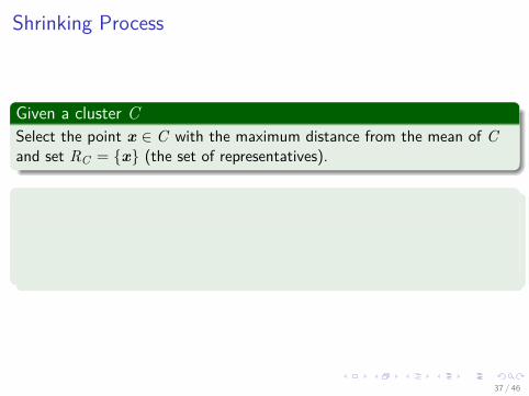
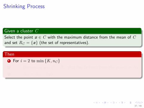
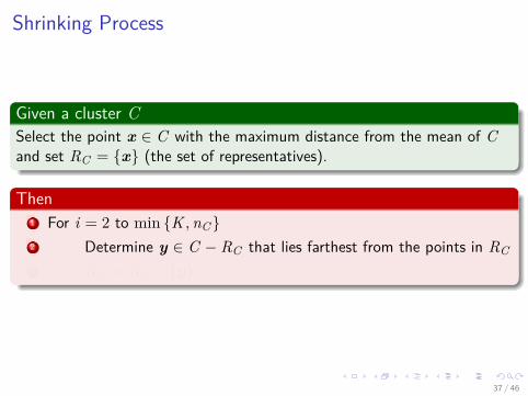
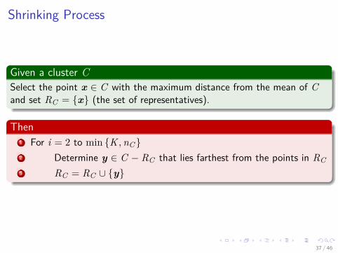
Given a cluster CSelect the point x ∈ C with the maximum distance from the mean of Cand set RC = {x} (the set of representatives).
Then1 For i = 2 to min {K ,nC}2 Determine y ∈ C − RC that lies farthest from the points in RC3 RC = RC ∪ {y}
37 / 46
Images/cinvestav-1.jpg
Shrinking Process
Given a cluster CSelect the point x ∈ C with the maximum distance from the mean of Cand set RC = {x} (the set of representatives).
Then1 For i = 2 to min {K ,nC}2 Determine y ∈ C − RC that lies farthest from the points in RC3 RC = RC ∪ {y}
37 / 46
Images/cinvestav-1.jpg
Shrinking Process
Given a cluster CSelect the point x ∈ C with the maximum distance from the mean of Cand set RC = {x} (the set of representatives).
Then1 For i = 2 to min {K ,nC}2 Determine y ∈ C − RC that lies farthest from the points in RC3 RC = RC ∪ {y}
37 / 46

Images/cinvestav-1.jpg
Shrinking Process
Given a cluster CSelect the point x ∈ C with the maximum distance from the mean of Cand set RC = {x} (the set of representatives).
Then1 For i = 2 to min {K ,nC}2 Determine y ∈ C − RC that lies farthest from the points in RC3 RC = RC ∪ {y}
37 / 46
Images/cinvestav-1.jpg
Shrinking Process
Given a cluster CSelect the point x ∈ C with the maximum distance from the mean of Cand set RC = {x} (the set of representatives).
Then1 For i = 2 to min {K ,nC}2 Determine y ∈ C − RC that lies farthest from the points in RC3 RC = RC ∪ {y}
37 / 46
Images/cinvestav-1.jpg
Shrinking Process
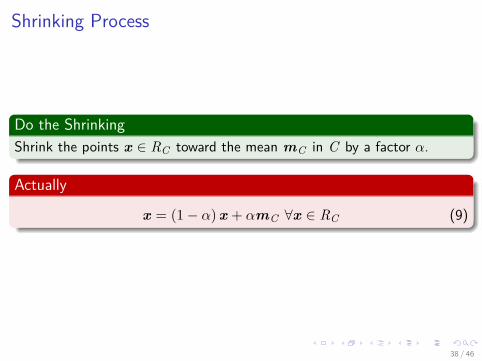
Do the ShrinkingShrink the points x ∈ RC toward the mean mC in C by a factor α.
Actually
x = (1− α) x + αmC ∀x ∈ RC (9)
38 / 46
Images/cinvestav-1.jpg
Shrinking Process
Do the ShrinkingShrink the points x ∈ RC toward the mean mC in C by a factor α.
Actually
x = (1− α) x + αmC ∀x ∈ RC (9)
38 / 46
Images/cinvestav-1.jpg
Resulting set RC
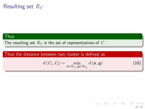
ThusThe resulting set RC is the set of representatives of C .
Thus the distance between two cluster is defined as
d (Ci ,Cj) = minx∈RCi ,y∈RCj
d (x,y) (10)
39 / 46
Images/cinvestav-1.jpg
Resulting set RC
ThusThe resulting set RC is the set of representatives of C .
Thus the distance between two cluster is defined as
d (Ci ,Cj) = minx∈RCi ,y∈RCj
d (x,y) (10)
39 / 46
Images/cinvestav-1.jpg
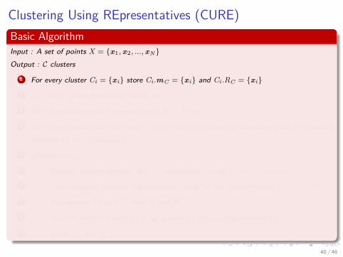
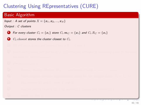
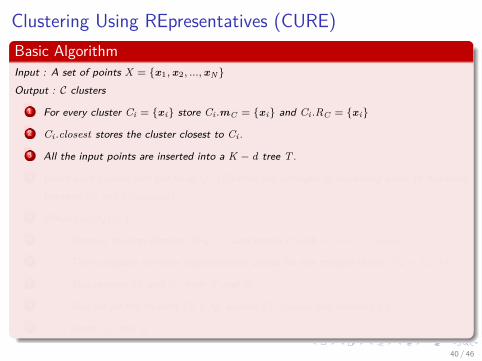
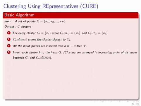
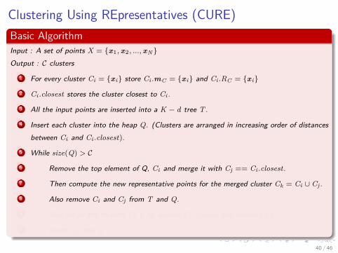
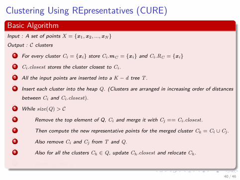
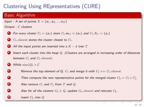
Clustering Using REpresentatives (CURE)Basic AlgorithmInput : A set of points X = {x1, x2, ..., xN}Output : C clusters
1 For every cluster Ci = {xi} store Ci .mC = {xi} and Ci .RC = {xi}
2 Ci .closest stores the cluster closest to Ci .
3 All the input points are inserted into a K − d tree T .
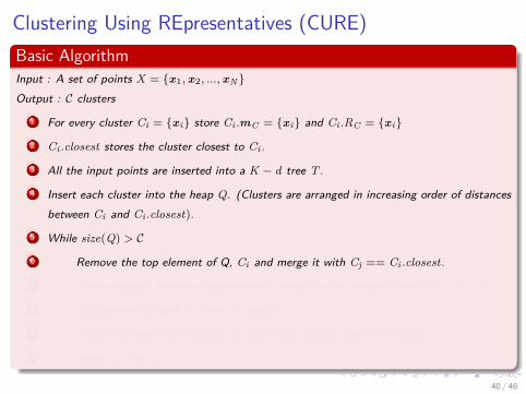
4 Insert each cluster into the heap Q. (Clusters are arranged in increasing order of distancesbetween Ci and Ci .closest).
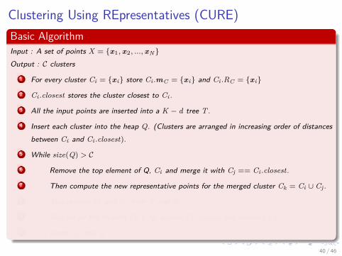
5 While size(Q) > C
6 Remove the top element of Q, Ci and merge it with Cj == Ci .closest.
7 Then compute the new representative points for the merged cluster Ck = Ci ∪ Cj .
8 Also remove Ci and Cj from T and Q.
9 Also for all the clusters Ch ∈ Q, update Ch .closest and relocate Ch .
10 insert Ck into Q
40 / 46
Images/cinvestav-1.jpg
Clustering Using REpresentatives (CURE)Basic AlgorithmInput : A set of points X = {x1, x2, ..., xN}Output : C clusters
1 For every cluster Ci = {xi} store Ci .mC = {xi} and Ci .RC = {xi}
2 Ci .closest stores the cluster closest to Ci .
3 All the input points are inserted into a K − d tree T .
4 Insert each cluster into the heap Q. (Clusters are arranged in increasing order of distancesbetween Ci and Ci .closest).
5 While size(Q) > C
6 Remove the top element of Q, Ci and merge it with Cj == Ci .closest.
7 Then compute the new representative points for the merged cluster Ck = Ci ∪ Cj .
8 Also remove Ci and Cj from T and Q.
9 Also for all the clusters Ch ∈ Q, update Ch .closest and relocate Ch .
10 insert Ck into Q
40 / 46
Images/cinvestav-1.jpg
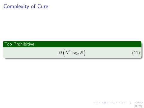
Complexity of Cure
Too Prohibitive
O(N 2 log2 N
)(11)
41 / 46
Images/cinvestav-1.jpg
Possible Solution
CURE does the followingThe technique adopted by the CURE algorithm, in order to reduce thecomputational complexity, is that of random sampling .
ActuallyThat is, a sample set X ′ is created from X , by choosing randomly N ′ outof the N points of X .
However, one has to ensure that the probability of missing a cluster ofX, due to this samplingThis can be guaranteed if the number of points N ′ is sufficiently large.
42 / 46
Images/cinvestav-1.jpg
Then
Having estimated N ′
CURE forms a number of p = NN ′ sample data sets by successive random
samples.
In other wordsIn other words, X is partitioned randomly in p subsets.
For this a parameter q is selectedThen, the points in each partition are clustered until N ′
q clusters areformed or the distance between the closest pair of clusters to be merged inthe next iteration step exceeds a user-defined threshold.
43 / 46
Images/cinvestav-1.jpg
Once this has been finished
A second clustering pass is doneOne the at most p N ′
q = Nq clusters from all the subsets.
The GoalTo apply the merging procedure described previously to all (at most) N
q sothat we end up with the required final number, m, of clusters.
FinallyEach point x in the data set, X , that is not used as a representative inany one of the m clusters is assigned to one of them according to thefollowing strategy.
44 / 46
Images/cinvestav-1.jpg
Finally
FirstA random sample of representative points from each of the m clusters ischosen.
ThenThen, based on the previous representatives the point x is assigned to thecluster that contains the representative closest to it.
Experiments reported by Guha et al. show that CUREIt is sensitive to parameter selection.
I Specifically K must be large enough to capture the geometry of eachcluster.
I In addition, N ′ must be higher than a certain percentage ≈ 2.5% of N .
45 / 46
Images/cinvestav-1.jpg
Not only that
The value of a affects also CURESmall values, CURE looks similar than a MST clustering.Large values, CURE resembles an algorithm with a singlerepresentative.
Worst Case Complexity
O(N ′2 log2 N ′
)(12)
46 / 46
Images/cinvestav-1.jpg
Not only that
The value of a affects also CURESmall values, CURE looks similar than a MST clustering.Large values, CURE resembles an algorithm with a singlerepresentative.
Worst Case Complexity
O(N ′2 log2 N ′
)(12)
46 / 46