2D PLOTTING

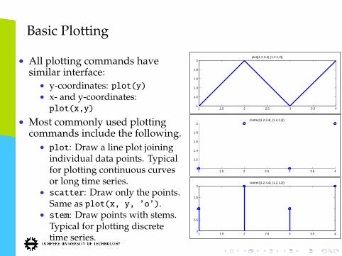
Basic Plotting

• All plotting commands havesimilar interface:• y-coordinates: plot(y)• x- and y-coordinates:plot(x,y)

• Most commonly used plottingcommands include the following.• plot: Draw a line plot joining

individual data points. Typicalfor plotting continuous curvesor long time series.

• scatter: Draw only the points.Same as plot(x, y, ’o’).

• stem: Draw points with stems.Typical for plotting discretetime series.

1 1.5 2 2.5 3 3.5 41

1.2

1.4

1.6

1.8

2plot([1,2,3,4], [1,2,1,2])

1 1.5 2 2.5 3 3.5 41

1.2

1.4

1.6

1.8

2scatter([1,2,3,4], [1,2,1,2])

1 1.5 2 2.5 3 3.5 40

0.5

1

1.5

2scatter([1,2,3,4], [1,2,1,2])

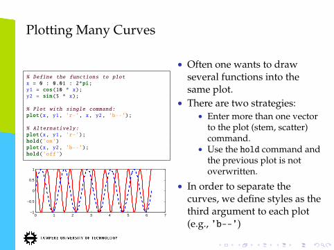
Plotting Many Curves

% Define the functions to plotx = 0 : 0.01 : 2*pi;y1 = cos(10 * x);y2 = sin(5 * x);

% Plot with single command:plot(x, y1, ’r-’, x, y2, ’b--’);

% Alternatively:plot(x, y1, ’r-’);hold(’on’)plot(x, y2, ’b--’);hold(’off’)

0 1 2 3 4 5 6 7−1

−0.5

0

0.5

1

• Often one wants to drawseveral functions into thesame plot.

• There are two strategies:• Enter more than one vector

to the plot (stem, scatter)command.

• Use the hold command andthe previous plot is notoverwritten.

• In order to separate thecurves, we define styles as thethird argument to each plot(e.g., ’b--’)

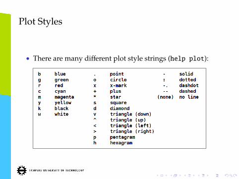
Plot Styles

• There are many different plot style strings (help plot):

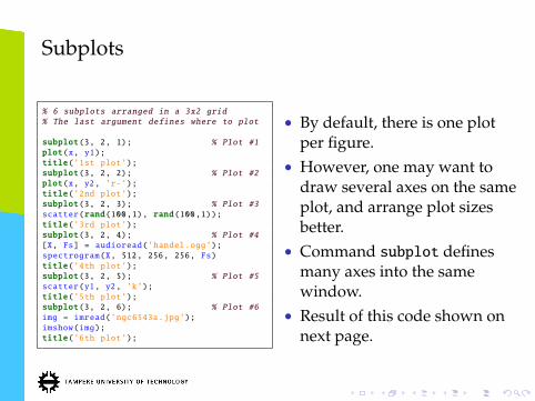
Subplots

% 6 subplots arranged in a 3x2 grid% The last argument defines where to plot

subplot(3, 2, 1); % Plot #1plot(x, y1);title(’1st plot’);subplot(3, 2, 2); % Plot #2plot(x, y2, ’r-’);title(’2nd plot’);subplot(3, 2, 3); % Plot #3scatter(rand(100,1), rand(100,1));title(’3rd plot’);subplot(3, 2, 4); % Plot #4[X, Fs] = audioread(’handel.ogg’);spectrogram(X, 512, 256, 256, Fs)title(’4th plot’);subplot(3, 2, 5); % Plot #5scatter(y1, y2, ’k’);title(’5th plot’);subplot(3, 2, 6); % Plot #6img = imread(’ngc6543a.jpg’);imshow(img);title(’6th plot’);

• By default, there is one plotper figure.

• However, one may want todraw several axes on the sameplot, and arrange plot sizesbetter.

• Command subplot definesmany axes into the samewindow.

• Result of this code shown onnext page.

Subplots

Annotations

plot(x, y1, ’g-’, x, y2, ’k--’)

axis([0, 2*pi, -1.5, 1.5]);legend({’Sine’, ’Cosine’});xlabel(’Time’);ylabel(’Oscillation’);title(’Two Oscillating

Functions’);annotation(’textarrow’, [0.4,

0.47], [0.2, 0.25], ’String’, ’Minimum value’);

grid(’on’);

0 1 2 3 4 5 6−1.5

−1

−0.5

0

0.5

1

1.5

Time

Osc

illat

ion

Two Oscillating Functions

SineCosine

Minimum value

• The subplots were markedwith a title on top of each plot.

• There are many otherannotation tools to add text,arrows, lines, legends, etc. onthe plot:• title: text above plot• xlabel: text for x-axis• ylabel: text for y-axis• legend: names for curves• grid: grid on and off• annotation: arrows, lines,

text, etc.

• Note: Annotations can also beinserted interactively fromfigure window.

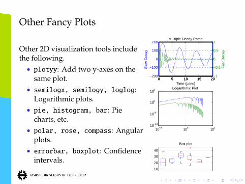
Other Fancy Plots

Other 2D visualization tools includethe following.• plotyy: Add two y-axes on the

same plot.• semilogx, semilogy, loglog:

Logarithmic plots.• pie, histogram, bar: Pie

charts, etc.• polar, rose, compass: Angular

plots.• errorbar, boxplot: Confidence

intervals.

0 5 10 15 20−200

−100

0

100

200Multiple Decay Rates

Time (µsec)

Slo

w D

ecay

0 5 10 15 20−1

−0.5

0

0.5

1

Fas

t Dec

ay

10−2 100 10210−10

10−5

100

105 Logarithmic Plot

10

20

30

40

Box plot

DATA IMPORT AND EXPORT

Importing Data

• Matlab has its own file format for storing data andvariables.

• However, not all applications produce Matlab compatiblefile formats.

• In such cases, a low level simple data format may berequired as an intermediate step (such as csv).

• Matlab has several utilities for importing data from widelyused formats.

Matlab Native File Format

% Save the entire workspace

>> X = [1;2;3];>> save data.mat % Save all variables>> clear all % Clear everything>> load data.mat % Load all variables>> disp(X)

123

% Save data into txt format.% Note: The variable names are not stored,% so recovery may be difficult.

>> save data.txt -ascii>> type data.txt

1.0000000e+002.0000000e+003.0000000e+00

% Save only variables X and Y:

>> save data.mat X Y

• Matlab has its own file formatthat can easily store andrecover the entire workspace.

• The default format is binaryfile, which may contain anyMatlab data type includingtheir names.

• When loaded, the values gettheir original names (this mayin fact be confusing).

• Variants of the save commandallow saving in ascii format.

• However, the ascii file doesnot store variable names.

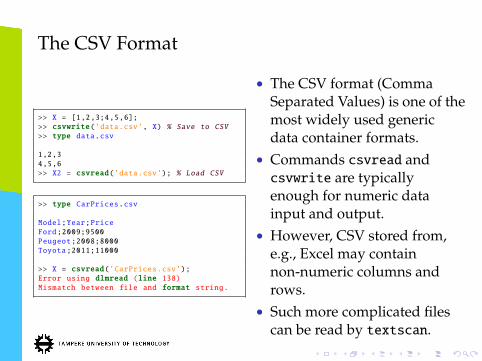
The CSV Format

>> X = [1,2,3;4,5,6];>> csvwrite(’data.csv’, X) % Save to CSV>> type data.csv

1,2,34,5,6>> X2 = csvread(’data.csv’); % Load CSV

>> type CarPrices.csv

Model;Year;PriceFord;2009;9500Peugeot;2008;8000Toyota;2011;11000

>> X = csvread(’CarPrices.csv’);Error using dlmread (line 138)Mismatch between file and format string.

• The CSV format (CommaSeparated Values) is one of themost widely used genericdata container formats.

• Commands csvread andcsvwrite are typicallyenough for numeric datainput and output.

• However, CSV stored from,e.g., Excel may containnon-numeric columns androws.

• Such more complicated filescan be read by textscan.

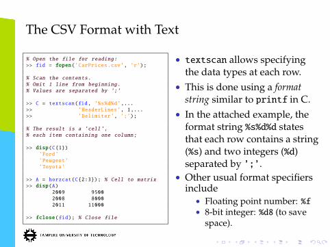
The CSV Format with Text

% Open the file for reading:>> fid = fopen(’CarPrices.csv’, ’r’);

% Scan the contents.% Omit 1 line from beginning.% Values are separated by ’;’

>> C = textscan(fid, ’%s%d%d’,...>> ’HeaderLines’, 1,...>> ’Delimiter’, ’;’);

% The result is a ’cell’,% each item containing one column;

>> disp(C{1})’Ford’’Peugeot’’Toyota’

>> A = horzcat(C{2:3}); % Cell to matrix>> disp(A)

2009 95002008 80002011 11000

>> fclose(fid); % Close file

• textscan allows specifyingthe data types at each row.

• This is done using a formatstring similar to printf in C.

• In the attached example, theformat string %s%d%d statesthat each row contains a string(%s) and two integers (%d)separated by ’;’.

• Other usual format specifiersinclude• Floating point number: %f• 8-bit integer: %d8 (to save

space).

The Excel Format

>> [num,txt,raw] = xlsread(’CarPrices.xlsx’)

num =

2009 95002008 80002011 11000

txt =

’Model’ ’Year’ ’Price’’Ford’ ’’ ’’’Peugeot’ ’’ ’’’Toyota’ ’’ ’’

raw =

’Model’ ’Year’ ’Price’’Ford’ [2009] [ 9500]’Peugeot’ [2008] [ 8000]’Toyota’ [2011] [11000]

• Excel files are wellsupported.

• Basic commands: xlsreadand xlswrite.

• The xls reader returnsthree outputs:• num: A matrix with all

numerical values found.• txt: A cell array with all

textual values found.• raw: A cell array with all

values found.

The HDF5 Format

% Load example HDF5 file that comes% with Matlab

>> info = h5info(’example.h5’)

info =

Filename: ’/matlab/demos/example.h5’Name: ’/’

Groups: [4x1 struct]Datasets: []Datatypes: []

Links: []Attributes: [2x1 struct]

>> info.Groups(:).Name

/g1

/g2

/g3

/g4

• Hierarchical Data Format(HDF) appears often withlarge datasets.

• Allows tree structuredstorage and access to thedata; resembling the unixdirectory tree.

• The example illustrates theuse of h5info commandthat is used for exploringthe file contents.

• In this case, the filecontains four datasetscalled g1,...,g4

The HDF5 Format

% See subsets of dataset number 2:

>> info.Groups(2).Datasets.Name

dset2.1

dset2.2

% Load the latter one

>> D = h5read(’example.h5’, ’/g2/dset2.2’)

D =

0 0 00.1000 0.2000 0.30000.2000 0.4000 0.60000.3000 0.6000 0.90000.4000 0.8000 1.2000

• The commands h5readand h5write take care ofreading and writing theHDF5 files.

• The only non-trivial thingis finding the correct "path"inside the file.

• However, the file hierarchyis usually described by theoriginal creator of the data.

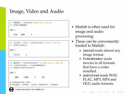
Image, Video and Audio

>> image = imread(’ngc6543a.jpg’);>> size(image)

ans =

650 600 3

>> [audio, Fs] = audioread(’handel.mp3’);>> size(audio)

ans =

73113 1

>> movie = VideoReader(’freqResponse.mp4’);>> videoFrames = read(movie);>> size(videoFrames)

ans =

900 1200 3 98

% Dimensions are:% height, width, color channels, frames

• Matlab is often used forimage and audioprocessing.

• These can be convenientlyloaded to Matlab:• imread reads almost any

image format.• VideoReader reads

movies in all formatsthat have a codecinstalled.

• audioread reads WAV,FLAC, MP3, MP4 andOGG audio formats.

Other Formats

Other supported formats include:• NetCDF Files (Network Common Data Form): scientific

data• CDF (Common Data Format): scientific data• XML (Extensible Markup Language): structured input and

output• DICOM (Digital Imaging and Communications in

Medicine): medical images• HDR (High Dynamic Range): images• Webcam: video from laptop camera• Other devices: See Data Acquisition Toolbox

PROGRAMMING

Programming

• When writing any program code longer than a few dozenlines, you will need functions.

• Next we will study how functions are implemented inMatlab.

Functions

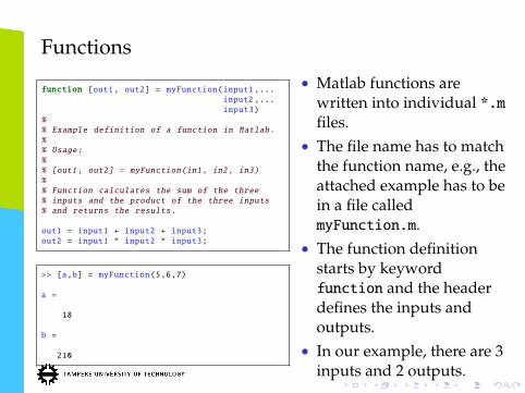
function [out1, out2] = myFunction(input1 ,...input2 ,...input3)

%% Example definition of a function in Matlab.%% Usage:%% [out1, out2] = myFunction(in1, in2, in3)%% Function calculates the sum of the three% inputs and the product of the three inputs% and returns the results.

out1 = input1 + input2 + input3;out2 = input1 * input2 * input3;

>> [a,b] = myFunction(5,6,7)

a =

18

b =

210

• Matlab functions arewritten into individual *.mfiles.

• The file name has to matchthe function name, e.g., theattached example has to bein a file calledmyFunction.m.

• The function definitionstarts by keywordfunction and the headerdefines the inputs andoutputs.

• In our example, there are 3inputs and 2 outputs.

Functions

function [out1, out2] = myFunction(input1 ,...input2 ,...input3)

%% Example definition of a function in Matlab.%% Usage:%% [out1, out2] = myFunction(in1, in2, in3)%% Function calculates the sum of the three% inputs and the product of the three inputs% and returns the results.

out1 = input1 + input2 + input3;out2 = input1 * input2 * input3;

>> help myFunctionExample definition of a function in Matlab.

Usage:

[out1, out2] = myFunction(in1, in2, in3)

Function calculates the sum of the threeinputs and the product of the three inputsand returns the results.

• Below the header is thedescription of using thefunction.

• This message is shownwhen help myFunction iscalled.

• Below the help message,the actual computation isdone.

• The return values aredetermined based on theheader: Whatever valuesare in out1 and out2 atexit, will be automaticallyreturned.

Variable Arguments

function result = myFunction(in1, in2,varargin)

% Usage:%% result = myFunction(in1, in2, [in3])%% Function calculates the sum of the two first% inputs optionally multiplies the sum with% the third.

if nargin == 3in3 = varargin{1};result = (in1 + in2) * in3;

elseresult = in1 + in2;

end

>> res = myFunction(5,6,7)

res =77

>> res = myFunction(5,6)

res =11

• It is possible to overloadthe function such that itcan accept variablenumber of arguments.

• This is done with thekeyword varargin as thelast item of the definition.

• After this, the variablesnargin contains thenumber of argumentswhen called.

• vararginwill be a cellarray of the extraarguments.

Omitting Arguments

% I want to calculate the spectrogram% of a signal with:%% spectrogram(X,WINDOW,NOVERLAP,NFFT,Fs)%% However, I only want to specify X and Fs.

[x, Fs] = audioread(’handel.ogg’);spectrogram(x, [], [], [], Fs);

• The varargin structureallows user to omit someoptional arguments.

• Sometimes you may wantto set the last argumentand omit some middleones.

• In this case, the emptymatrix can be given inplace of omittedarguments.

Example: Search for the Root of a Function

% Define a function handle for our target:

>> func = @(x) cos(x.^2);

% Now we can call the function as usual.% Let’s plot it.

>> x = 0:0.01:10;>> plot(x, func(x));

0 1 2 3 4 5 6 7 8 9 10−1

−0.5

0

0.5

1Function cos(x2)

• Let’s implement a longerfunction, which searchesfor the root of a givenfunction.

• We will use bisection searchalgorithm, which starts attwo sides of the root andhalves the range at eachiteration.

• Question: How to pass thetarget function to ourprogram?

• Answer: We use a functionhandle defined by ’@’.

Bisection Search

The bisection algorithm works as follows.

Iterate until finished:

1 Assume x1 and x2 are at opposite sides of the root, suchthat f(x1) and f(x2) have different signs.

2 Check the sign at the center: x0 = (x1 + x2)/2:• If f(x1) and f(x0) have different signs, then root is in [x1, x0].

Set x2 = x0.• If f(x2) and f(x0) have different signs, then root is in [x0, x2].

Set x1 = x0.

3 Go to step 1.

Example: Search for the Root of a Function

function x = searchRoot(f, x1, x2)

% Find the root of function f using thebisection method.

%% Usage:%% x = searchRoot(f, x1, x2)%% x1 and x2 have to be such that x1*x2 < 0

half = (x1+x2) / 2;

% Assert that f has different sign in x1and x2

if sign(f(x1)) == sign(f(x2))x = half;return

end

% Check if we’re already close enoughto the root

if abs(f(half)) < 1e-5x = half;return

end

% Make sure x1 < x2

if x1 > x2tmp = x1;x1 = x2;x2 = tmp;

end

% Otherwise , check the sign at half andrecurse

if sign(f(half)) == sign(f(x1))x = searchRoot(f, half, x2);

elsex = searchRoot(f, half, x1);

end

Example: Search for the Root of a Function

0 1 2 3 4 5 6 7 8 9 10−1

−0.5

0

0.5

1Function cos(x2)

func = @(x) cos(x.^2);x0 = searchRoot(func, 1, 2);

0 2 4 6 8 10 12 14 161.25

1.3

1.35

1.4

1.45

1.5

Iteration

• For our function, it seemsthat locations x1 = 1 andx2 = 2 are good startingpoints.

• The function iterates for 16rounds and reachesx0 = 1.2533 for whichf(x0) = 0.00000747.

Debugging

• Debugging helps in finding bugs in the code.• Matlab editor allows setting breakpoints, where execution

stops.

• Breakpoint is set by pressing F12 when on the active line.

Debugging

• When executed, the program flow will stop at breakpoint.• Moving mouse over variables will show their values.• The Matlab prompt is also available.

• Shortcuts: F5 = run forward, F10 = step to next line,F11 = enter inside function, shift + F5 = stop