Empirical Bayes Moderation ofAsymptotically Linear Parameters

Nima Hejazi

Division of BiostatisticsUniversity of California, Berkeleystat.berkeley.edu/~nhejazi

nimahejazi.orgtwitter/@nshejazi

github/nhejazi

slides: goo.gl/6ou8YR

These are slides for a talk given most recently at the Division ofBiostatistics seminar series, at the University of California, Berkeleyon 20 March 2017.

Source: https://github.com/nhejazi/talk_biotmleSlides: https://goo.gl/r3zsu6With notes: https://goo.gl/6ou8YR

Preview

1. Linear models are the standard approach foranalyzing microarray and next-generationsequencing data (e.g., R package “limma”).

2. Moderated statistics help reduce false positives byusing an empirical Bayes method to perform standarddeviation shrinkage for test statistics.

3. Beyond linear models: we can assess evidence usingparameters that are more scientifically interesting(e.g., ATE) by way of TMLE.

4. The approach of moderated statistics easily extendsto the case of asymptotically linear parameters.

1

We’ll go over this summary again at the end of the talk. Hopefully, itwill all make more sense then.

Motivation: Let’s meet the data▶ Observational study of the impact of occupational

exposure (to benzene), with data collected on 125subjects and roughly 22,000 biomarkers.

▶ Biomarkers of interest are in the form of miRNA,assessed using the Illumina Human Ref-8 BeadChipsplatform.

▶ Occupational exposure to benzene reported asdiscrete values of interest (to epidemiologists): none,< 1ppm, > 5ppm.

▶ Background (phenotype-level) information availableon each subject, including age, sex, smoking status.

2

This is not an atypical data set by modern standards in epidemiology,certainly not the standard for molecular biology. That is, sample sizesare usually much smaller in experiments examining biologicalprocesses.

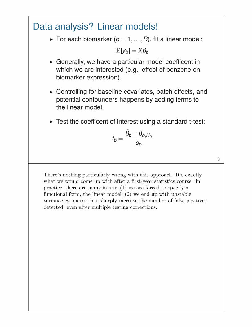
Data analysis? Linear models!▶ For each biomarker (b = 1, . . . ,B), fit a linear model:

E[yb] = Xβb

▶ Generally, we have a particular model coefficent inwhich we are interested (e.g., effect of benzene onbiomarker expression).

▶ Controlling for baseline covariates, batch effects, andpotential confounders happens by adding terms tothe linear model.

▶ Test the coefficent of interest using a standard t-test:

tb =β̂b −βb,H0

sb

3

There’s nothing particularly wrong with this approach. It’s exactlywhat we would come up with after a first-year statistics course. Inpractice, there are many issues: (1) we are forced to specify afunctional form, the linear model; (2) we end up with unstablevariance estimates that sharply increase the number of false positivesdetected, even after multiple testing corrections.

LIMMA: Linear Models for Microarray Data▶ When the sample size is small, s2

b may be so smallthat small differences (β̂b −βb,H0) lead to large tb.

▶ Uncertainty in the variance is an acute problem whenthe sample size is small.

▶ This results in false positives. Smyth proposes we getaround this by an empirical Bayes shrinkage of the s2

b.

▶ Test the coefficent of interest with a moderated t-test:

t̃b =β̂b −βb,H0

s̃b, s̃2

b =s2

bdb +s20d0

db +d0

▶ Eliminates large t-statistics merely from very small sb.

4

The substantive contribution here is the use of an empirical Bayesmethod to shrink the standard deviation across all of the biomarkerssuch that we obtain a larger (but accurate) estimate that reduces thenumber of test statistics that are marked as significant by low s2

bestimates alone.

Note that this is not the exact formulation of the moderatedt-statistic as given by Smyth (his derivation assumes a hierarchicalmodel; see original paper if interested). This formulation does a goodenough job to help us see the bigger picture.

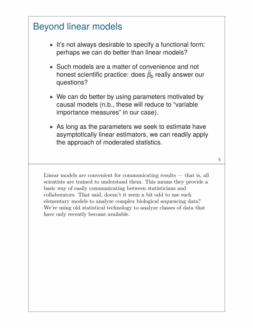
Beyond linear models▶ It’s not always desirable to specify a functional form:

perhaps we can do better than linear models?

▶ Such models are a matter of convenience and nothonest scientific practice: does β̂b really answer ourquestions?

▶ We can do better by using parameters motivated bycausal models (n.b., these will reduce to “variableimportance measures” in our case).

▶ As long as the parameters we seek to estimate haveasymptotically linear estimators, we can readily applythe approach of moderated statistics.

5

Linear models are convenient for communicating results — that is, allscientists are trained to understand them. This means they provide abasic way of easily communicating between statisticians andcollaborators. That said, doesn’t it seem a bit odd to use suchelementary models to analyze complex biological sequencing data?We’re using old statistical technology to analyze classes of data thathave only recently become available.

Target parameters for complex questions▶ Rather than being satisfied with β̂b as an answer to

our questions, let’s consider a simple targetparameter: the average treatment effect (ATE):Ψb(P0) = EW,0[E0[Yb | A = ahigh,W]−E0[Yb | A = alow,W]]

▶ No need to specify a functional form or assume thatwe know the true data-generating distribution P0.

▶ Parameters like this can be estimated using targetedminimum loss-based estimation (TMLE).

▶ Asymptotic linearity:

Ψb(P∗n)−Ψb(P0) =

1n

n∑i=1

IC(Oi)+oP(1√n

)

6

By allowing scientific questions to inform the parameters that wechoose to estimate, we can do a better job of actually answering thequestions of interest to our collaborators. Further, we abandon theneed to specify the functional relationship between our outcome andcovariates; moreover, we can now make use of advances in machinelearning.

Targeted Minimum Loss-Based Estimation▶ TMLE produces a well-defined, unbiased, efficient

substitution estimator of target parameters of adata-generating distribution.

▶ Iterative procedure (though there is a one-step now)that updates an initial estimate of the relevant part(Q0) of the data generating distribution (P0).

▶ Like corresponding A-IPTW estimators, removesasymptotic residual bias of initial estimator for thetarget parameter. If it uses a consistent estimator ofg0 (nuisance parameter), it is doubly robust.

▶ We can estimate the target parameter:

Ψb(P∗n) =

1n

n∑i=1

[Q(b,1)n (Ai = ah,Wi)−Q(b,1)

n (Ai = al,Wi)]7

Natural use of machine learning methods for the estimation of bothQ0 and g0. Focuses effort to achieve minimal bias and asymptoticsemiparametric efficiency bound for the variance, but still getinference (with some assumptions).

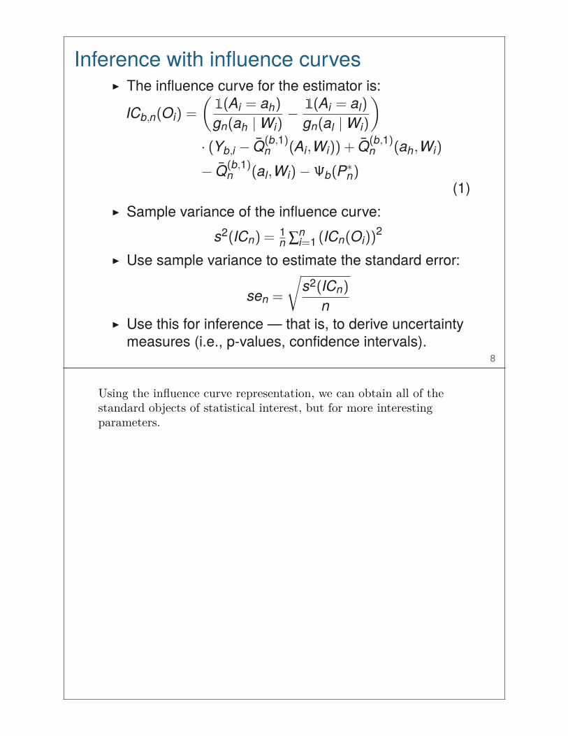
Inference with influence curves▶ The influence curve for the estimator is:

ICb,n(Oi) =

(1(Ai = ah)

gn(ah | Wi)− 1(Ai = al)

gn(al | Wi)

)

· (Yb,i − Q̄(b,1)n (Ai,Wi)) + Q̄(b,1)

n (ah,Wi)

− Q̄(b,1)n (al,Wi) − Ψb(P∗

n)(1)

▶ Sample variance of the influence curve:s2(ICn) = 1

n ∑ni=1 (ICn(Oi))

2

▶ Use sample variance to estimate the standard error:

sen =

√s2(ICn)

n▶ Use this for inference — that is, to derive uncertainty

measures (i.e., p-values, confidence intervals).8

Using the influence curve representation, we can obtain all of thestandard objects of statistical interest, but for more interestingparameters.

Moderated statistics for target parameters▶ One can define a standard t-test statistic for an

estimator of an asymptotically linear parameter (overb = 1, . . . ,B) as:

tb =

√n(Ψb(P∗

n)−Ψ0)

sb(ICb,n)

▶ This naturally extends to the moderated t-statistic ofSmyth:

t̃b =

√n(Ψb(P∗

n)−Ψ0)

s̃bwhere the posterior estimate of the variance of theinfluence curve is

s̃2b =

s2b(ICb,n)db +s2

0d0db +d0

9

• Consider this is repeated for b = 1, . . . ,B different biomarkers, sothat one has, for each b:

Ψb(Q∗b,n),S2

b(ICb,n),

estimate of variable importance and standard error for all B.

• Propose an existing joint-inferential procedure that can addsome finite-sample robustness to an estimator that can be highlyvariable.

An influence curve transform▶ Need the estimate for each biomarker (b) and the IC

for every observation for that biomarker, repeating forall b = 1, . . . ,B.

▶ Essentially, transform original data matrix such thatnew entries are:

Y∗b,i = ICb,n(Oi;Pn)+Ψb(P∗

n)

▶ Since E[ICb,n] = 0 across the columns (units) for eachb, the average will be the original estimate Ψb(P∗

n).

▶ For simplicity, let’s assume the null value is Ψ0 = 0 forall b. Then, applying the moderated t-test to Y∗

b,i willgenerate corrected, conservative test statistics t̃b.

10

Just like the one-sample problem for estimation of parameter withassociated standard error from the influence curve.

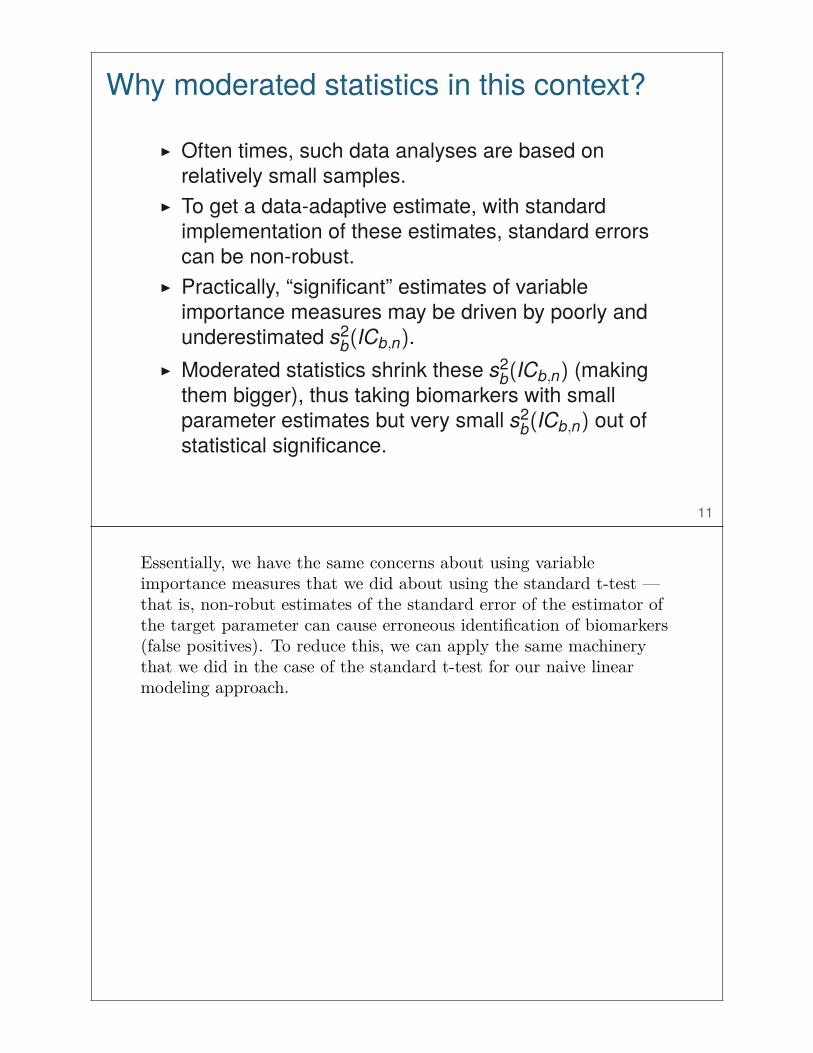
Why moderated statistics in this context?

▶ Often times, such data analyses are based onrelatively small samples.

▶ To get a data-adaptive estimate, with standardimplementation of these estimates, standard errorscan be non-robust.

▶ Practically, “significant” estimates of variableimportance measures may be driven by poorly andunderestimated s2

b(ICb,n).▶ Moderated statistics shrink these s2

b(ICb,n) (makingthem bigger), thus taking biomarkers with smallparameter estimates but very small s2

b(ICb,n) out ofstatistical significance.

11

Essentially, we have the same concerns about using variableimportance measures that we did about using the standard t-test —that is, non-robut estimates of the standard error of the estimator ofthe target parameter can cause erroneous identification of biomarkers(false positives). To reduce this, we can apply the same machinerythat we did in the case of the standard t-test for our naive linearmodeling approach.

Software implementation: “R/biotmle”▶ An R package that “facilitates biomarker discovery by

generalizing the moderated t-statistic of Smyth foruse with asymptotically linear parameters.”

▶ Check it out on GitHub: nhejazi/biotmle

12

Use it. File an issue. Help make it better!

Data analysis with “R/biotmle”▶ Observational study of the impact of occupational

exposure (to benzene), with data collected on 125subjects and roughly 22,000 biomarkers.

▶ Baseline covariates W: age, sex, smoking status; allwere discretized.

▶ Treatment A is degree of Benzene exposure: none,< 1ppm, and > 5ppm.

▶ Outcome Y is miRNA expression, median normalized.

▶ Estimate the parameter:Ψb(P∗

n) = E[E[Yb | A = max(A),W]−E[Yb | A = min(A),W]]

▶ Apply moderated t-test as previously discussed.13

We are really just walking through the mechanistic procedure weoutline, applying to the data set that served as our motivatingexample.

Analysis results I: Uncorrected tests

0

2000

4000

6000

8000

0.00 0.25 0.50 0.75 1.00

magnitude of raw p−values

coun

t

2000

4000

6000

8000

Histogram of raw p−values (applying Limma shrinkage to TMLE results)

14

This is promising — we’re not seeing too many biomarkers identifiedas “significant.” But, we do have to correct for those 22,000 teststhat we just performed.

Analysis results II: Corrected tests

0

5000

10000

15000

0.00 0.25 0.50 0.75 1.00

magnitude of BH−corrected p−values

coun

t

4000

8000

12000

16000

Histogram of FDR−corrected p−values (BH) (applying Limma shrinkage to TMLE results)

15

After application of the Benjamini-Hochberg procedure for controllingthe False Discovery Rate (FDR).

Analysis results III: Volcano plot

16

Taking a look at a standard volcano plot adapted to the ATE quicklyreveals that we really are not identifying any biomarkers with low foldchange in the ATE as significant erroneously.

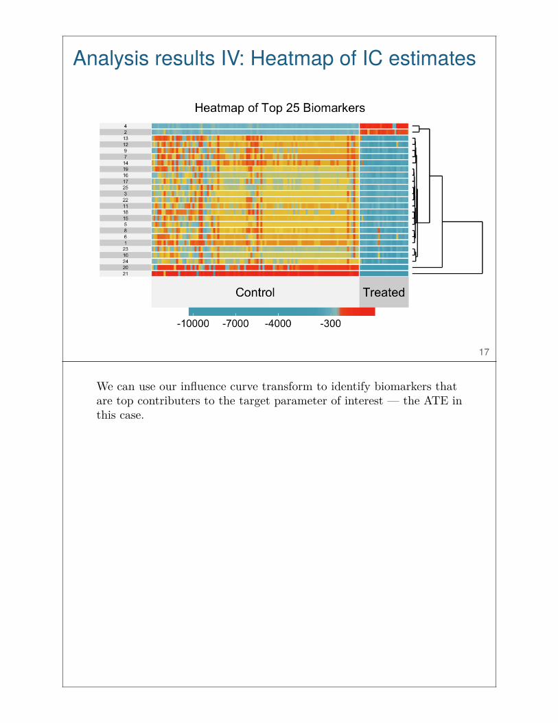
Analysis results IV: Heatmap of IC estimates

17

We can use our influence curve transform to identify biomarkers thatare top contributers to the target parameter of interest — the ATE inthis case.

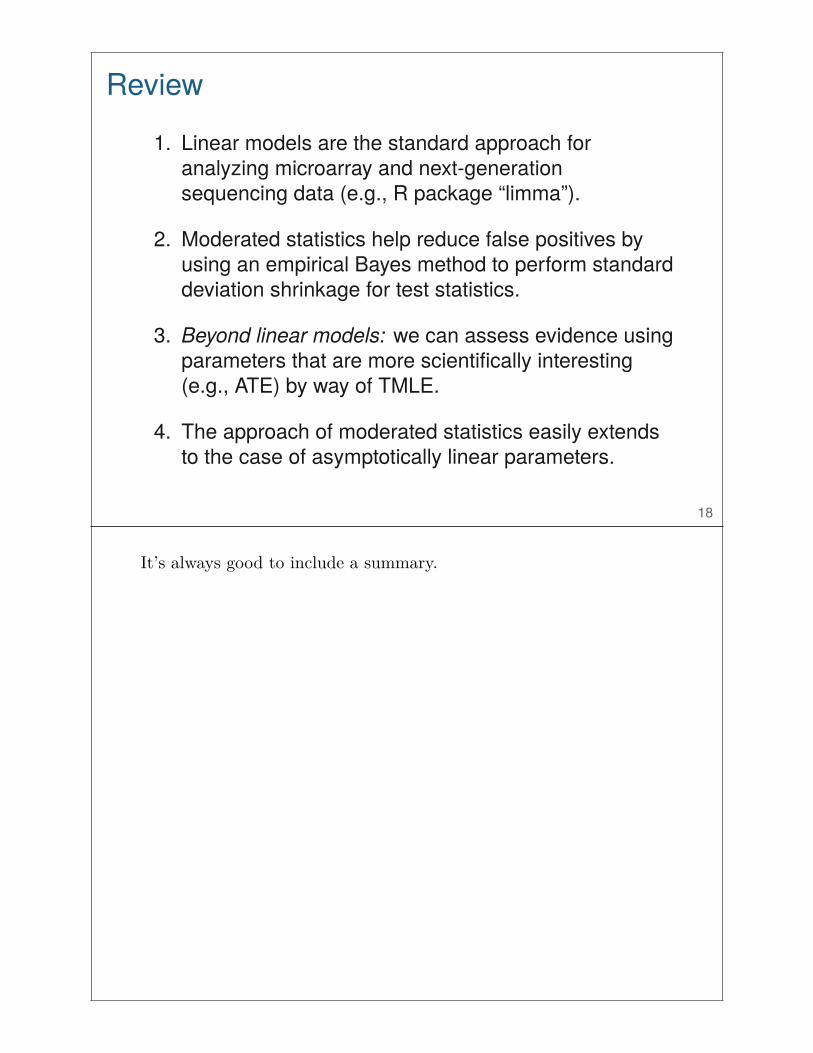
Review

1. Linear models are the standard approach foranalyzing microarray and next-generationsequencing data (e.g., R package “limma”).

2. Moderated statistics help reduce false positives byusing an empirical Bayes method to perform standarddeviation shrinkage for test statistics.

3. Beyond linear models: we can assess evidence usingparameters that are more scientifically interesting(e.g., ATE) by way of TMLE.

4. The approach of moderated statistics easily extendsto the case of asymptotically linear parameters.

18

It’s always good to include a summary.

References IBenjamini, Y. and Hochberg, Y. (1995). Controlling the

false discovery rate: a practical and powerful approachto multiple testing. Journal of the royal statistical society.Series B (Methodological), pages 289–300.

Gruber, S. and van der Laan, M. J. (2010). An applicationof collaborative targeted maximum likelihood estimationin causal inference and genomics. The InternationalJournal of Biostatistics, 6(1):1–31.

Hejazi, N. S., Cai, W., and Hubbard, A. E. (2017). biotmle:Targeted learning for biomarker discovery.

Smyth, G. K. (2004). Linear models and empirical bayesmethods for assessing differential expression inmicroarray experiments. Statistical Applications inGenetics and Molecular Biology, 3(1):1–25.

19

References II

Smyth, G. K. (2005). Limma: linear models for microarraydata. In Bioinformatics and computational biologysolutions using R and Bioconductor, pages 397–420.Springer.

Tuglus, C. and van der Laan, M. J. (2011). Targetedmethods for biomarker discovery. In Targeted Learning,pages 367–382. Springer.

van der Laan, M. J. and Rose, S. (2011). Targetedlearning: causal inference for observational andexperimental data. Springer Science & Business Media.

20

Acknowledgments

Alan Hubbard University of California, Berkeley

Mark van der Laan University of California, Berkeley

21

This was all made possible by generous advising and collaboration.

Slides: goo.gl/6ou8YR

stat.berkeley.edu/~nhejazi

nimahejazi.org

twitter/@nshejazi

github/nhejazi

22

Here’s where you can find me, as well as the slides for this talk.