3-1

Image Enhancement

• The goal of image enhancement is to improve the usefulness of an image for a given task, such as providing a more subjectively pleasing image for human viewing.

• In image enhancement, little or no attempt is made to estimate the actual image degradation process, and the techniques are often ad hoc. Image enhancement usually involves:

• Contrast manipulation

• Sharpening

• Noise reduction

3-2

Contrast Manipulation

3-3

Contrast Manipulation

• One of the most common defects of photographic or electronic images is poor contrast resulting from either

• Poor lighting conditions (e.g., an underexposed or an overexposed scene), or

• Sensor (capture medium) nonlinearity or small dynamic range compared to the dynamic range of the captured scene (e.g., back-lit scene).

• Image contrast can often be improved by a look-up table (LUT) operation that rescales the amplitude of each pixel. For example, in an underexposed image with the histogram centered around small codevalues, a LUT that stretches that range can result in the desired image enhancement.

3-4

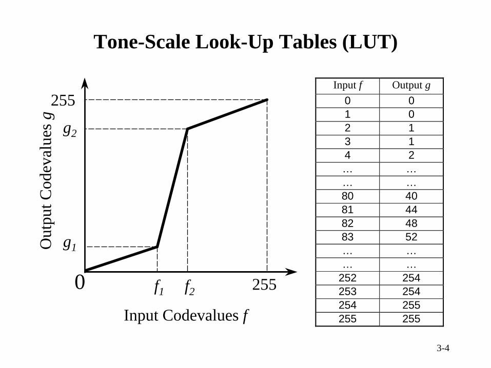
Tone-Scale Look-Up Tables (LUT)

Input f Output g 0 0 1 0 2 1 3 1 4 2 … … … … 80 40 81 44 82 48 83 52 … … … …

252 254 253 254 254 255 255 255

0

255

255

Input Codevalues f

Out

put C

odev

alue

s g

g2

f2

g1

f1

3-5

3-6

Phot

osho

p “C

urve

s”

3-7

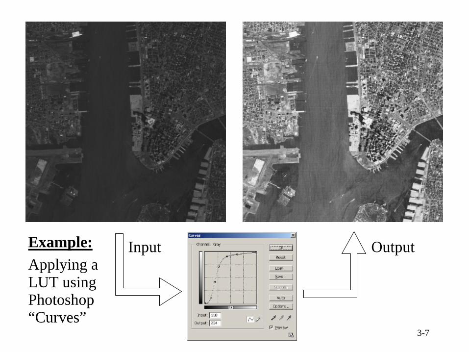
Example:Applying a LUT using Photoshop “Curves”

Input Output

3-8

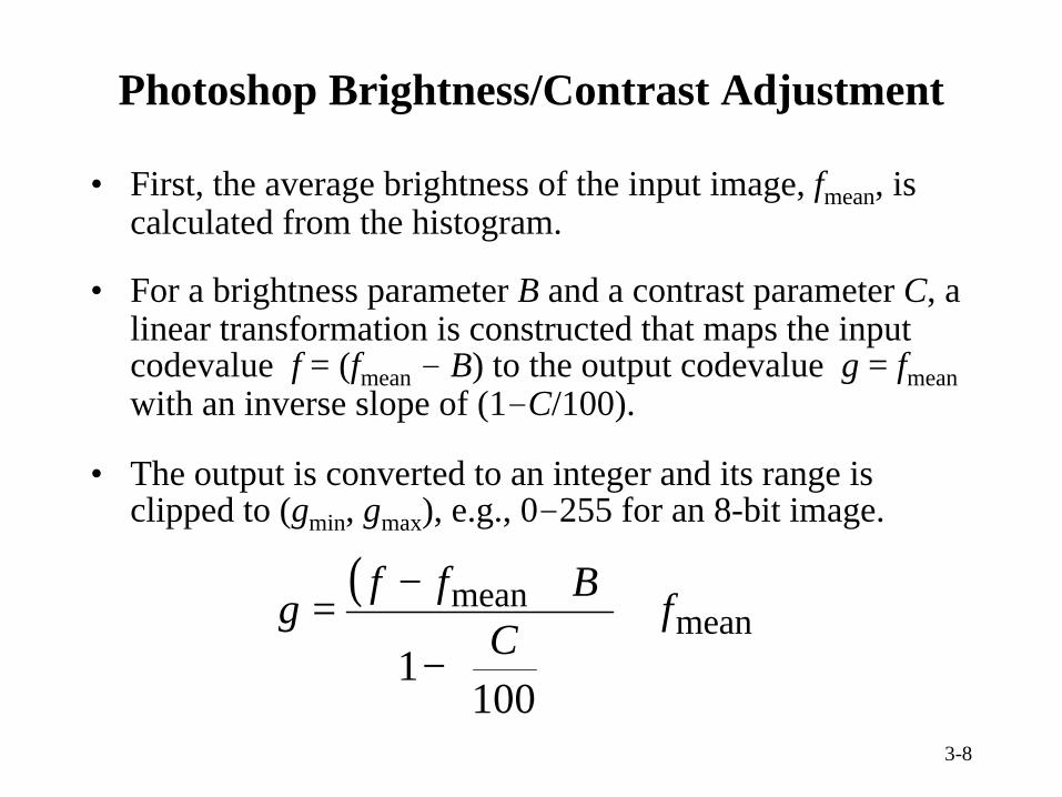
Photoshop Brightness/Contrast Adjustment

• First, the average brightness of the input image, fmean, is calculated from the histogram.

• For a brightness parameter B and a contrast parameter C, a linear transformation is constructed that maps the input codevalue f = (fmean - B) to the output codevalue g = fmeanwith an inverse slope of (1-C/100).

• The output is converted to an integer and its range is clipped to (gmin, gmax), e.g., 0-255 for an 8-bit image.

( )mean

mean

1001

fC

Bffg +

−

+−=

3-9

Photoshop Brightness/Contrast Adjustment

0

gmax

Input Codevalues f →

Out

put C

odev

alue

s g

→

gmin

fmean

Slope =

−

1001

1C

(fmean-B)

3-10

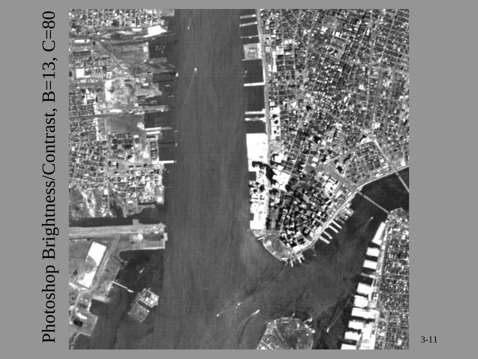
3-11Phot

osho

p B

righ

tnes

s/C

ontr

ast,

B=1

3, C

=80

3-12

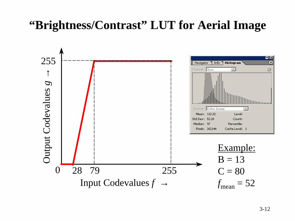
“Brightness/Contrast” LUT for Aerial Image

0

255

2557928

Example:B = 13C = 80fmean = 52Input Codevalues f →

Out

put C

odev

alue

s g

→

3-13

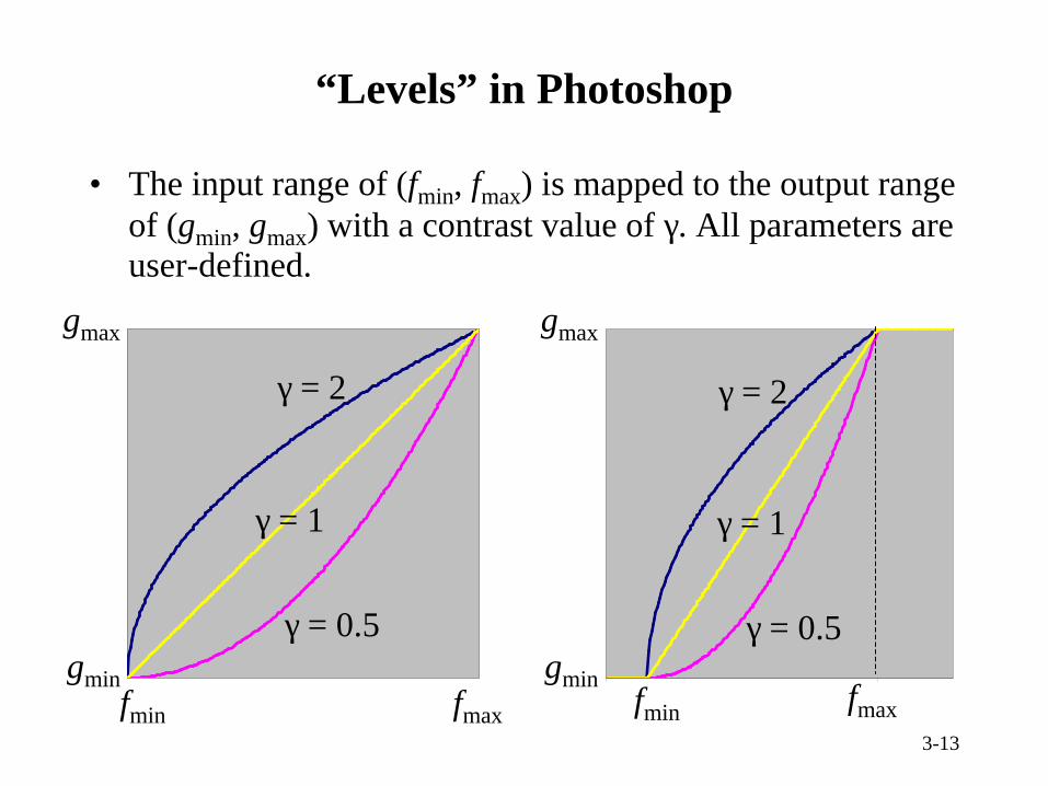
“Levels” in Photoshop

• The input range of (fmin, fmax) is mapped to the output range of (gmin, gmax) with a contrast value of γ. All parameters are user-defined.

fmin fmax

gmin

gmax

gmin

gmax

fmin fmax

γ = 1

γ = 2

γ = 0.5

γ = 1

γ = 2

γ = 0.5

3-14

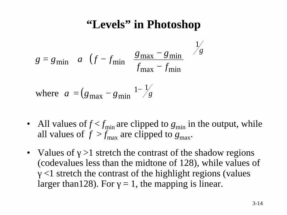
“Levels” in Photoshop

• All values of f < fmin are clipped to gmin in the output, while all values of f > fmax are clipped to gmax.

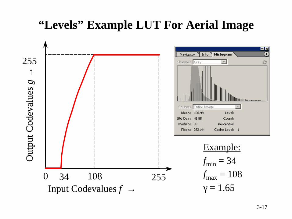
• Values of γ >1 stretch the contrast of the shadow regions(codevalues less than the midtone of 128), while values of γ <1 stretch the contrast of the highlight regions (values larger than128). For γ = 1, the mapping is linear.

( )γ

α

1

minmax

minmaxminmin

−−

−+=ffgg

ffgg

( ) γα11

minmax where −−= gg

3-15

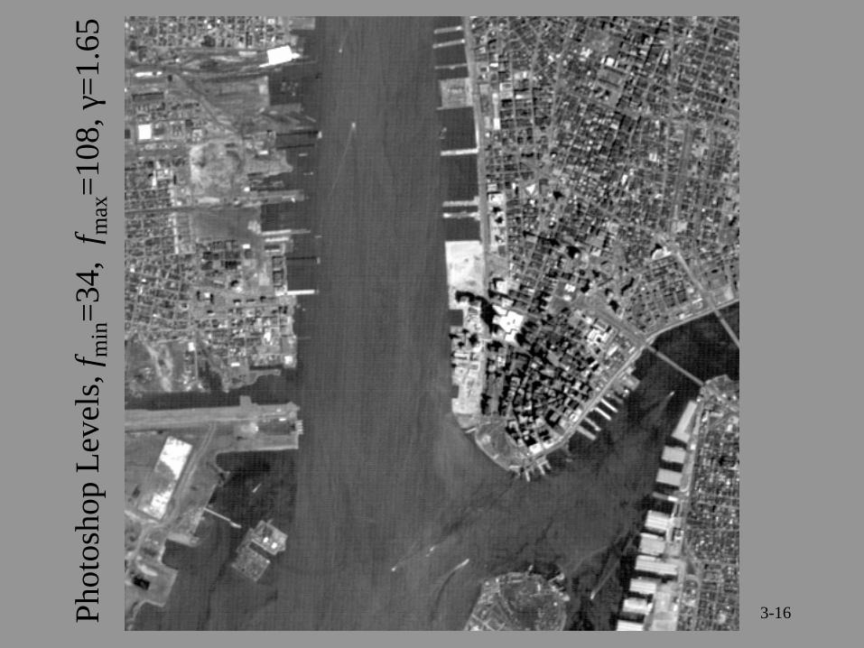
3-16Phot

osho

p L

evel

s, f m

in=3

4, f

max

=108

, γ=1

.65

3-17

“Levels” Example LUT For Aerial Image

0

255

25510834

Out

put C

odev

alue

s g

→

Input Codevalues f →

Example:fmin = 34fmax = 108γ = 1.65

3-18

Automatic Tone-Scale Modification

• In order to improve the system throughput and reduce costs, it is desirable to perform the tone-scale modification automatically.

• In general, the outcome of an automatic tone-scale operation will not be as robust as that of a manual one.

• Most automatic tone-scale operations are histogram based. Examples are:

• Auto Levels as used in Photoshop.

• Histogram Equalization as available in most image editing software packages.

3-19

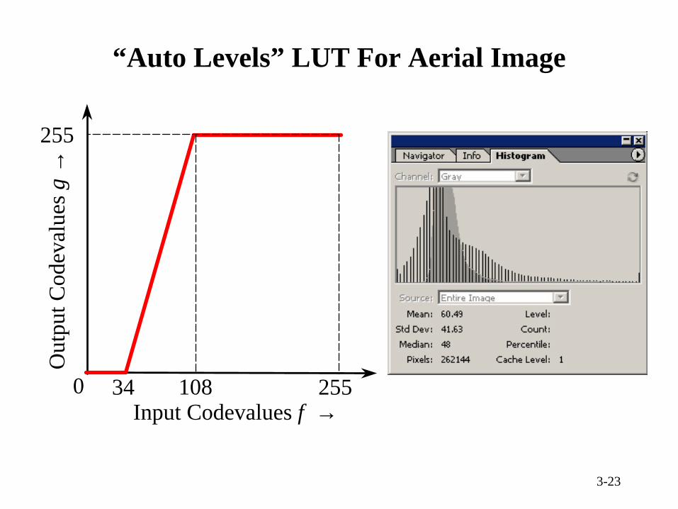
“Auto Levels” in Photoshop

• The two codevalues fmin and fmax in the original image are determined such that x% of the pixels have a codevalue less than or equal to fmin while y% of the pixels have acodevalue larger than or equal to fmax.

• The values of x and y are defined by the user and correspond, respectively, to the clip points for the dark regions (shadows) and the bright regions (highlights).

• For example, for Photoshop 7.0 the default values are x = y= 0.50, hence the range of (fmin, fmax) contains 99% of the input pixels. In Photoshop CS, the default values are x = y= 0.10. The default values can be changed by the user.

3-20

“Auto Levels” in Photoshop

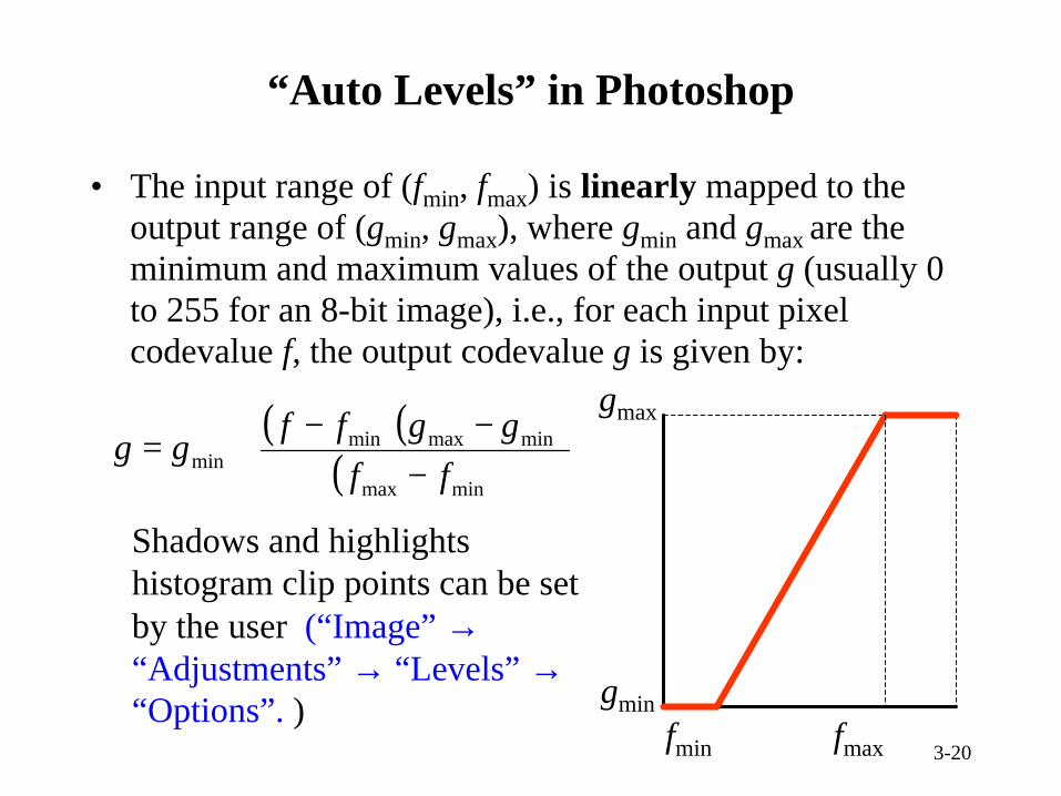
• The input range of (fmin, fmax) is linearly mapped to the output range of (gmin, gmax), where gmin and gmax are the minimum and maximum values of the output g (usually 0 to 255 for an 8-bit image), i.e., for each input pixelcodevalue f, the output codevalue g is given by:

( )( )( )minmax

minmaxminmin ff

ggffgg

−−−

+=

fmin fmax

gmin

gmax

Shadows and highlights histogram clip points can be set by the user (“Image” →“Adjustments” → “Levels” →“Options”. )

3-21

3-22

Phot

osho

p A

uto

Lev

els

3-23

“Auto Levels” LUT For Aerial Image

0

255

25510834

Out

put C

odev

alue

s g

→

Input Codevalues f →

3-24

Histogram Equalization

• Histogram Equalization (HE) is a look-up-table (LUT) operation that attempts to improve the contrast by redistributing the histogram in a roughly uniform fashion.

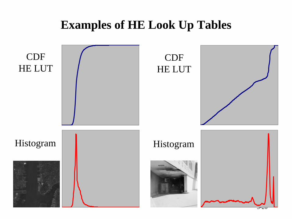
• It is done automatically and the resulting nonlinear LUT is derived from the histogram of the image. The slope of the LUT for a given input codevalue is proportional to the value of the histogram at that codevalue.

• In nonadaptive or global HE, the same LUT is utilized to process the entire image. This is useful for images that have an overall low contrast (e.g., underexposed or overexposed images). As in any LUT operation, HE often reduces the total number of output levels, so it may not be suitable for archiving applications.

3-25

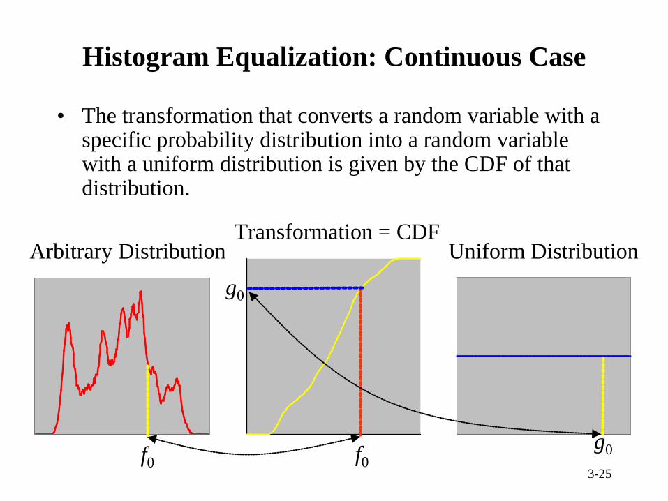
Histogram Equalization: Continuous Case

• The transformation that converts a random variable with a specific probability distribution into a random variable with a uniform distribution is given by the CDF of that distribution.

f0 f0

g0

g0

Arbitrary Distribution Uniform DistributionTransformation = CDF

3-26

Examples of HE Look Up Tables

Histogram

CDFHE LUT

Histogram

CDFHE LUT

3-27

Histogram Equalization: Discrete Case

• For the discrete HE case, for each input codevalue f, the output codevalue g is given by:

( ) )(CDFminmaxmin fgggg ×−+=

( )

∑

×−+= =

total

f

lf

N

lhgggg 0

minmaxmin

)(NINT

• Ntotal is the total number of pixels in the image, hf (l) is the input image histogram at codevalue l, and NINT denotes the operation of rounding to the nearest integer.

3-28

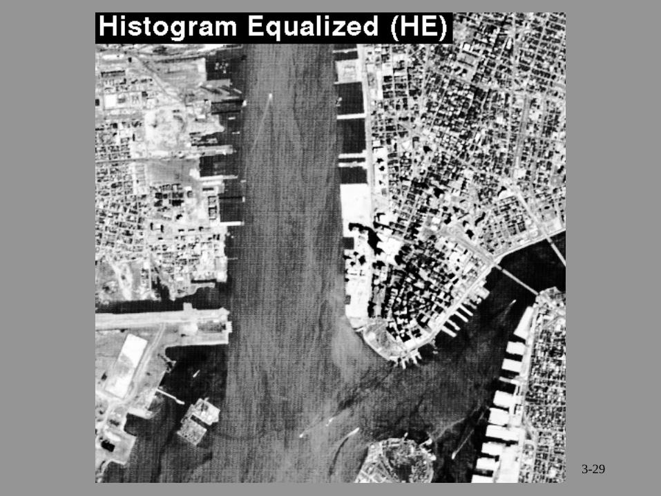
3-29

3-30

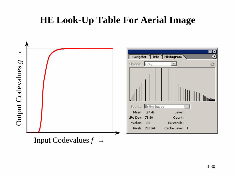
HE Look-Up Table For Aerial ImageO

utpu

t Cod

eval

ues

g →

Input Codevalues f →

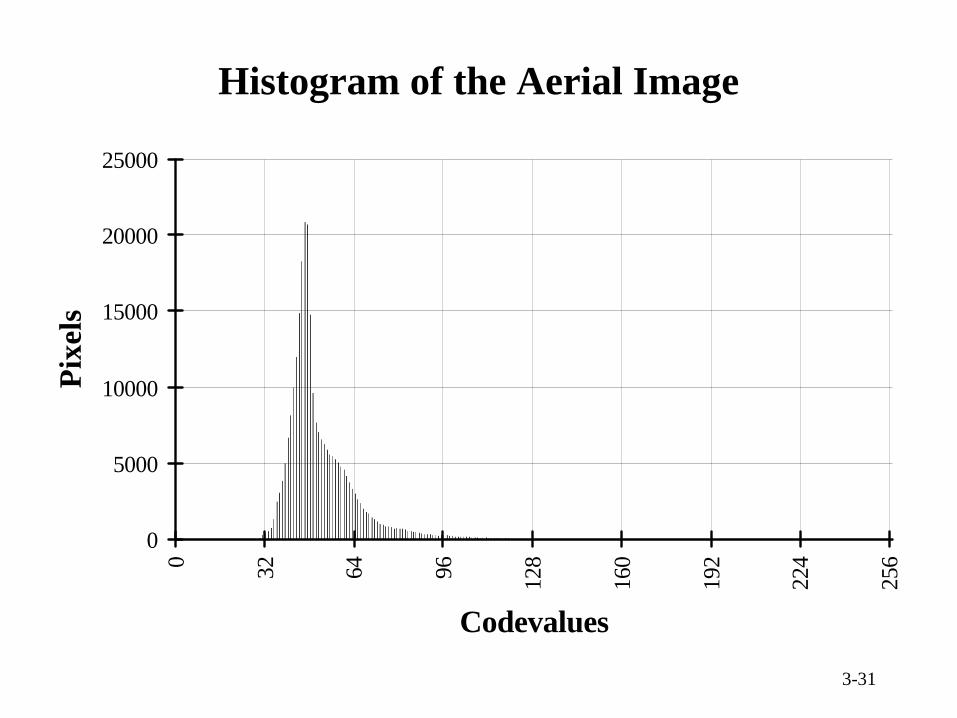
3-31

Histogram of the Aerial Image

0

5000

10000

15000

20000

250000 32 64 96 128

160

192

224

256

Codevalues

Pix

els

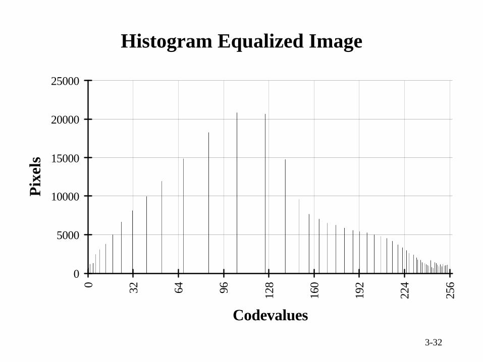
3-32

Histogram Equalized Image

0

5000

10000

15000

20000

250000 32 64 96 128

160

192

224

256

Codevalues

Pix

els

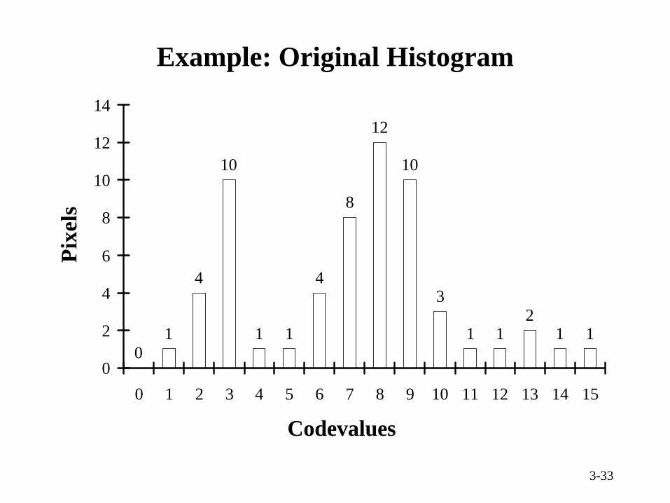
3-33

Example: Original Histogram

01

4

10

1 1

4

8

12

10

3

1 12

1 1

0

2

4

6

8

10

12

14

0 1 2 3 4 5 6 7 8 9 10 11 12 13 14 15

Codevalues

Pix

els

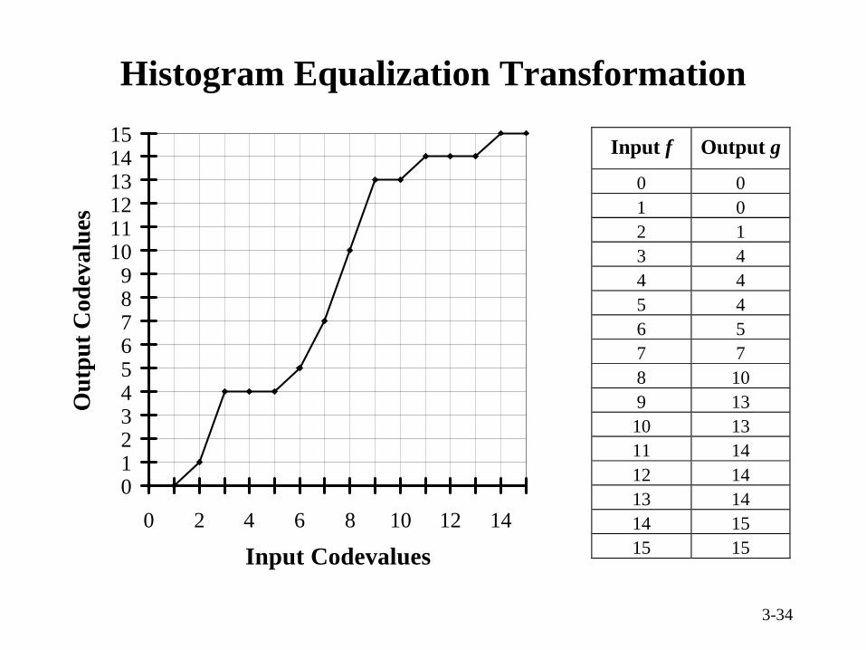
3-34

Histogram Equalization Transformation

Input f Output g

0 0 1 0 2 1 3 4 4 4 5 4 6 5 7 7 8 10 9 13 10 13 11 14 12 14 13 14 14 15 15 15

0123456789

101112131415

0 2 4 6 8 10 12 14

Input Codevalues

Out

put C

odev

alue

s

3-35

Equalized Histogram

1

4

0 0

12

4

0

8

0 0

12

0 0

13

4

2

0

2

4

6

8

10

12

14

0 1 2 3 4 5 6 7 8 9 10 11 12 13 14 15

Codevalues

Pix

els

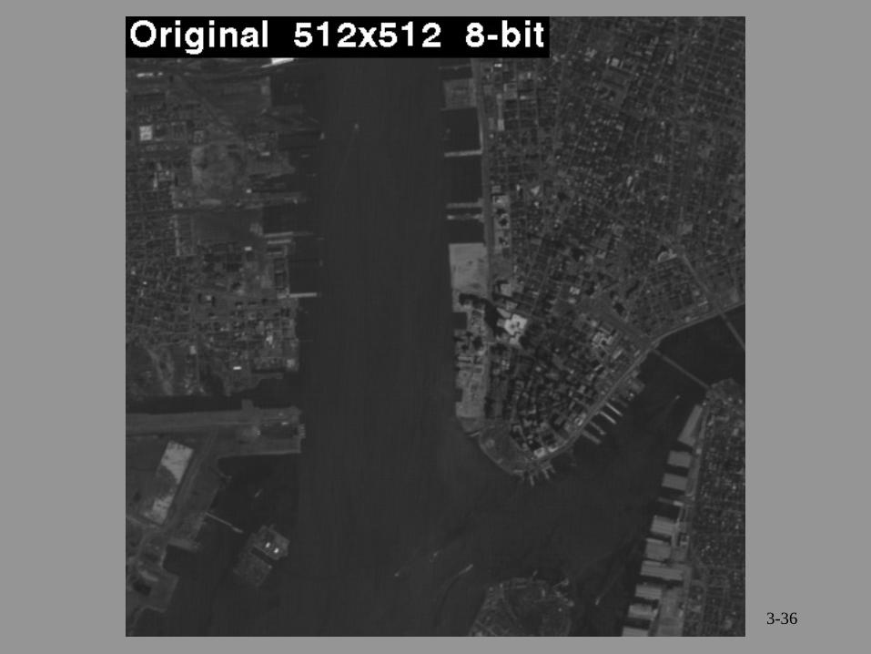
3-36

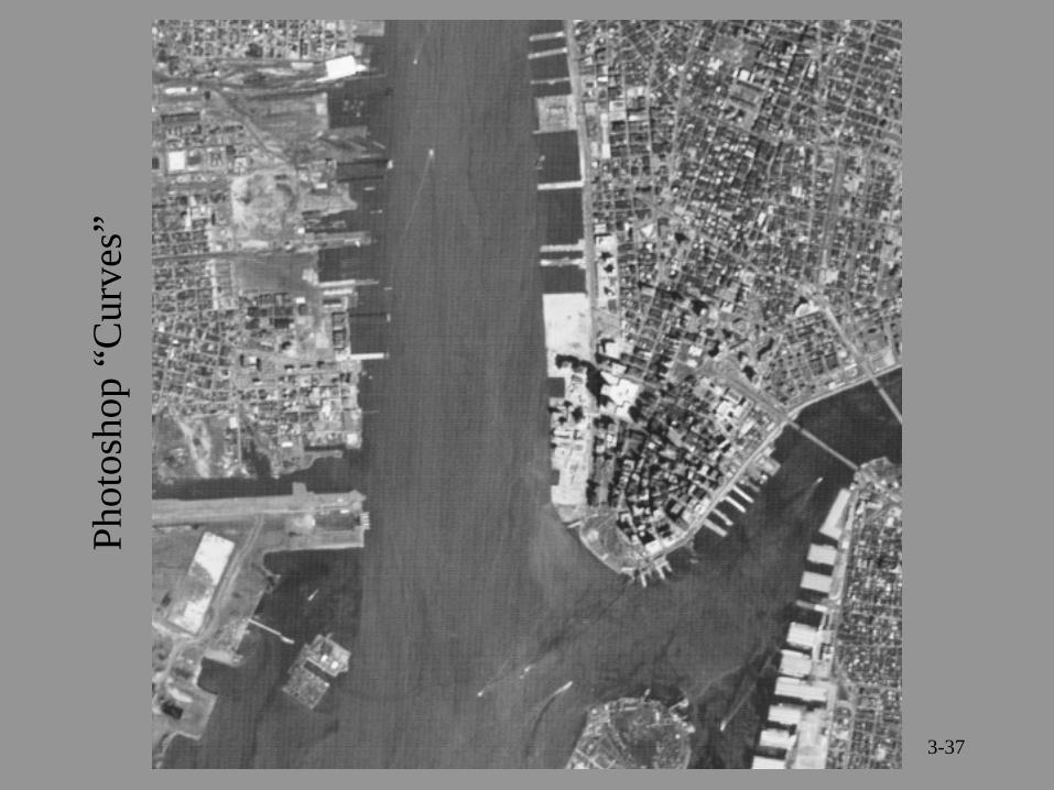
3-37

Phot

osho

p “C

urve

s”

3-38Phot

osho

p B

righ

tnes

s/C

ontr

ast,

B=1

3, C

=80

3-39Phot

osho

p L

evel

s, f m

in=3

4, f

max

=108

, γ=1

.65

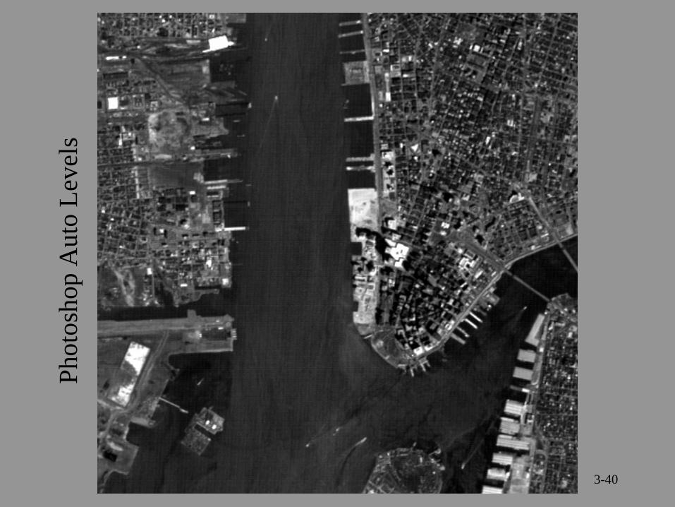
3-40

Phot

osho

p A

uto

Lev

els

3-41

3-42

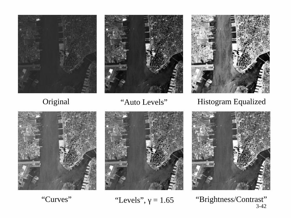
Original “Auto Levels” Histogram Equalized

“Curves” “Levels”, γ = 1.65 “Brightness/Contrast”

3-43

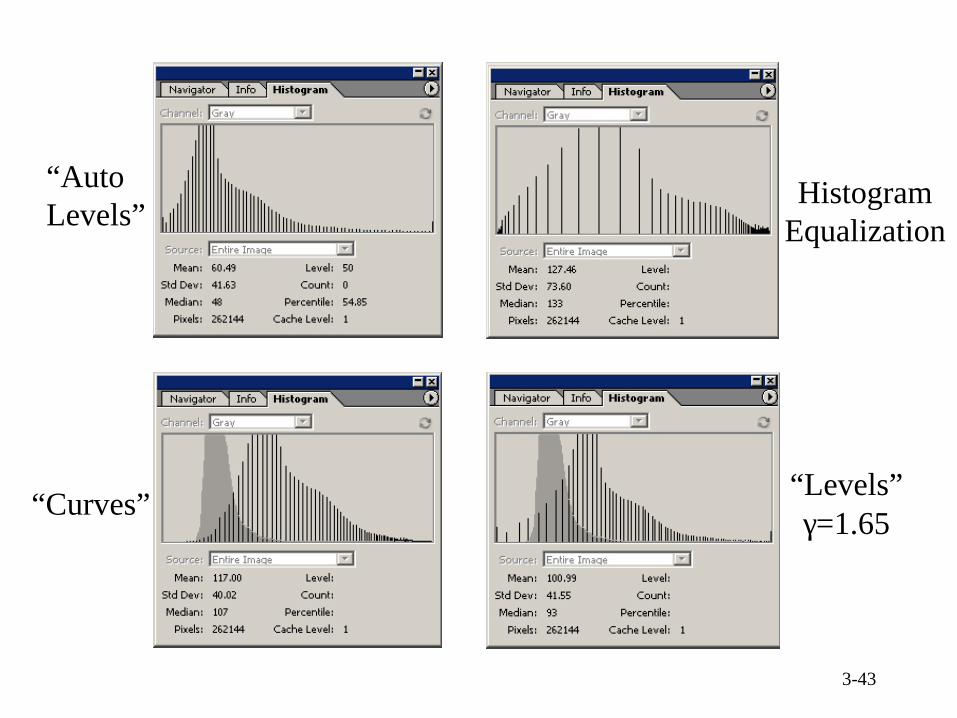
“Auto Levels”

“Curves”

Histogram Equalization

“Levels”γ=1.65

3-44

Histogram Equalization Considerations

In the process of HE, gray levels can only be merged but not broken up, so the histogram equalized image will have at most the same number of levels as the original image. In fact, it will often have less levels.

• It is advantageous to capture the original image with more bits/pixel.

• Sometimes large ranges of gray levels at the ends of the gray scale are mapped into a single level. It may thus be preferable to transform into a histogram that somewhat rolls off at the ends of the scale.

• To preserve the maximum information for image archiving applications, it may be preferable not to perform any type of LUT operation.

3-45

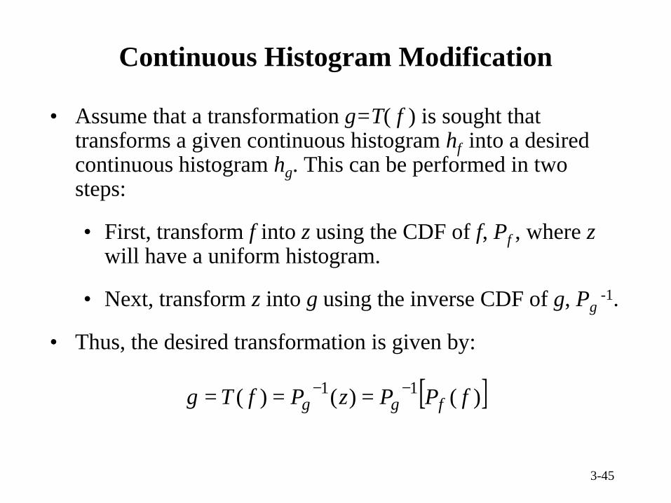
Continuous Histogram Modification

• Assume that a transformation g=T( f ) is sought that transforms a given continuous histogram hf into a desired continuous histogram hg. This can be performed in two steps:

• First, transform f into z using the CDF of f, Pf , where zwill have a uniform histogram.

• Next, transform z into g using the inverse CDF of g, Pg-1.

• Thus, the desired transformation is given by:

[ ])()()( 11 fPPzPfTg fgg−− ===

3-46

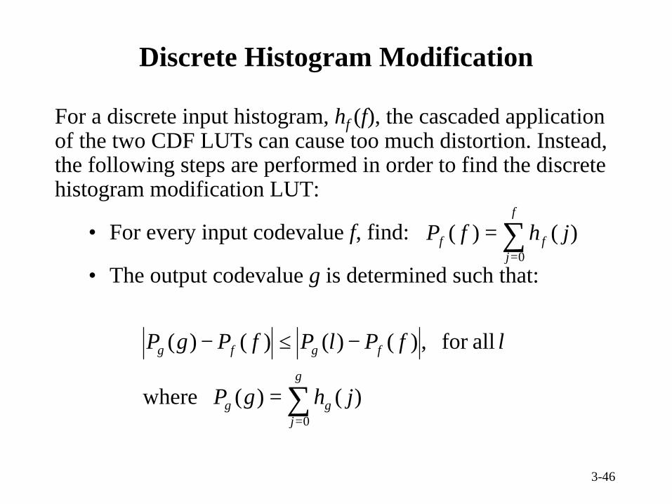
Discrete Histogram Modification

For a discrete input histogram, hf (f), the cascaded application of the two CDF LUTs can cause too much distortion. Instead, the following steps are performed in order to find the discrete histogram modification LUT:

• For every input codevalue f, find:

• The output codevalue g is determined such that:

∑=

=

−≤−g

jgg

fgfg

jhgP

lfPlPfPgP

0

)()( where

allfor ,)()()()(

∑=

=f

jff jhfP

0

)()(

3-47

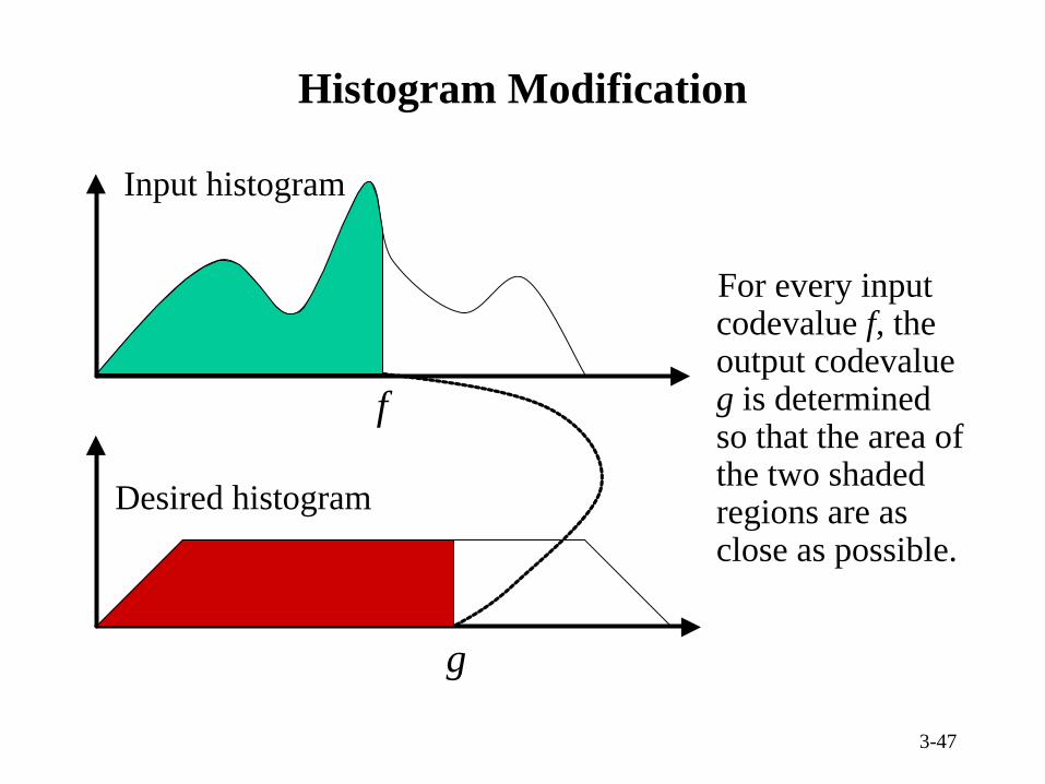
Histogram Modification

f

g

For every input codevalue f, the output codevalue g is determined so that the area of the two shaded regions are as close as possible.

Input histogram

Desired histogram

3-48

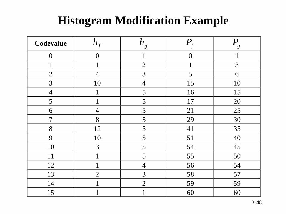
Histogram Modification Example

Codevalue h f hg Pf Pg

0 0 1 0 11 1 2 1 32 4 3 5 63 10 4 15 104 1 5 16 155 1 5 17 206 4 5 21 257 8 5 29 308 12 5 41 359 10 5 51 4010 3 5 54 4511 1 5 55 5012 1 4 56 5413 2 3 58 5714 1 2 59 5915 1 1 60 60

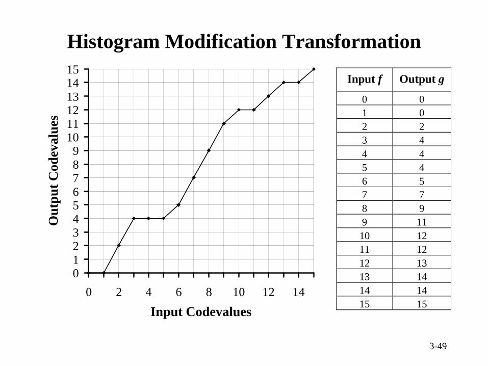
3-49

Histogram Modification Transformation

Input f Output g

0 0 1 0 2 2 3 4 4 4 5 4 6 5 7 7 8 9 9 11

10 12 11 12 12 13 13 14 14 14 15 15

0123456789

101112131415

0 2 4 6 8 10 12 14

Input Codevalues

Out

put C

odev

alue

s

3-50

Modified Histogram

10

4

0

12

4

0

8

0

12

0

10

4

1

3

1

0

2

4

6

8

10

12

14

0 1 2 3 4 5 6 7 8 9 10 11 12 13 14 15

Codevalues

Pix

els

3-51

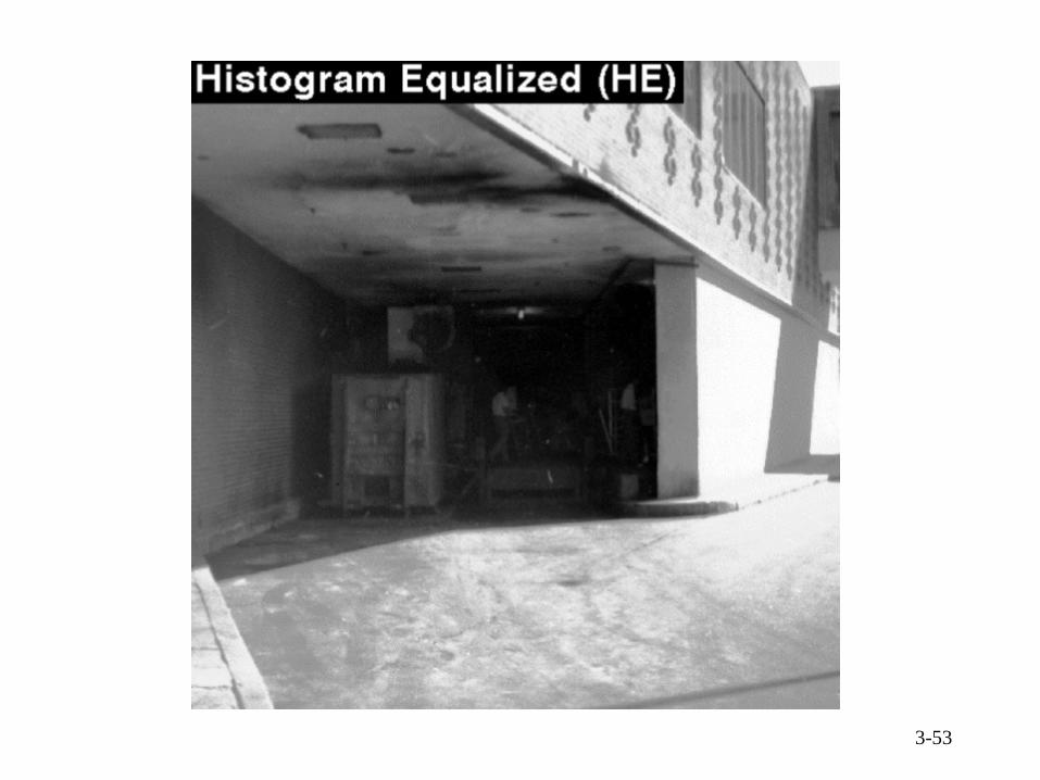
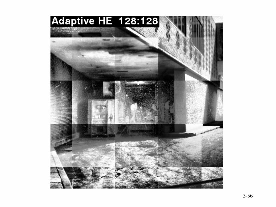
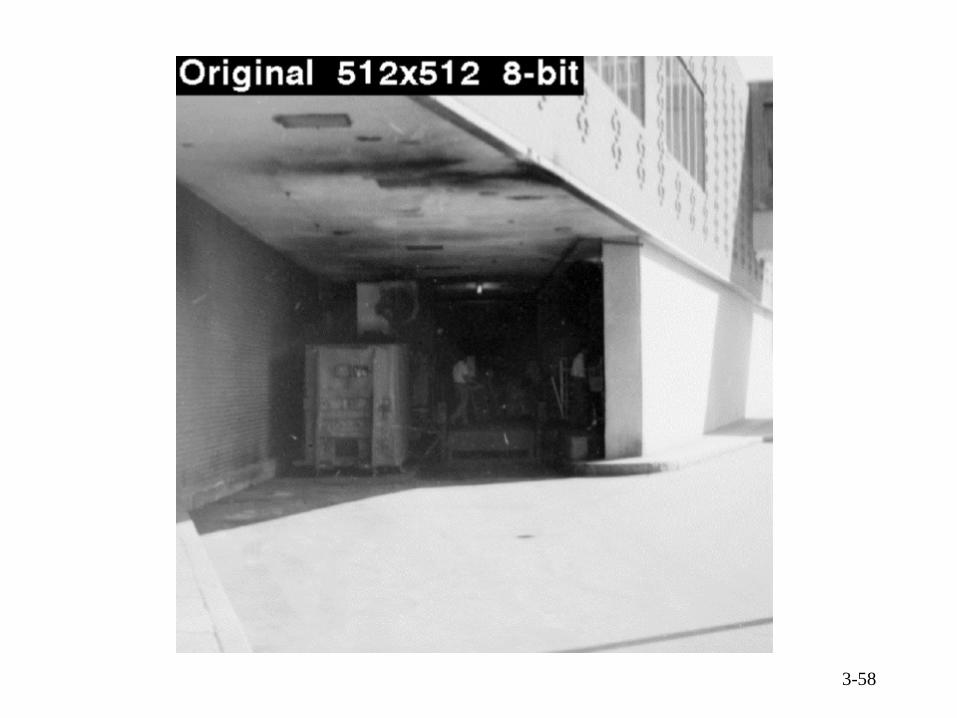
Adaptive Histogram Equalization

• Sometimes the overall histogram of an image may have a wide distribution while the histogram of its local regions are highly skewed. In such cases, it is often desirable to enhance the contrast of these local regions. This is performed by adaptive histogram equalization (AHE).

• The term adaptive implies that different regions of the image are processed differently (e.g., with different look-up tables). AHE is applied in an automatic fashion, however, because of its additional computational complexity, it may not be implementable in real-time.

• AHE can be used to create an effect similar to the dodging and burning performed in conventional darkrooms.

3-52

3-53

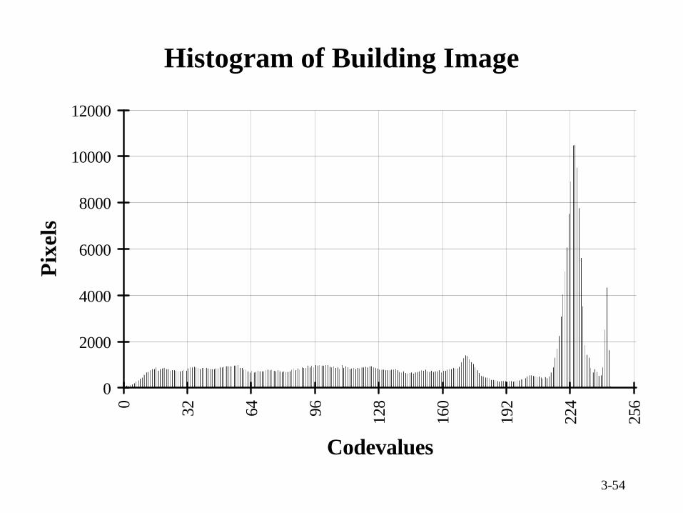
3-54

Histogram of Building Image

0

2000

4000

6000

8000

10000

120000 32 64 96 128

160

192

224

256

Codevalues

Pix

els

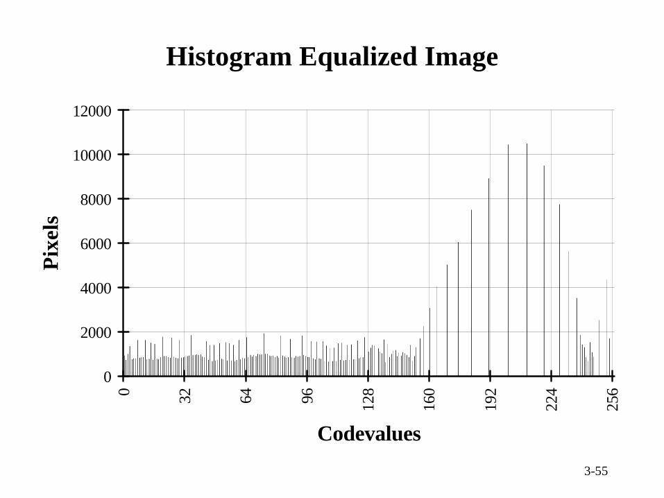
3-55

Histogram Equalized Image

0

2000

4000

6000

8000

10000

120000 32 64 96 128

160

192

224

256

Codevalues

Pix

els

3-56

3-57

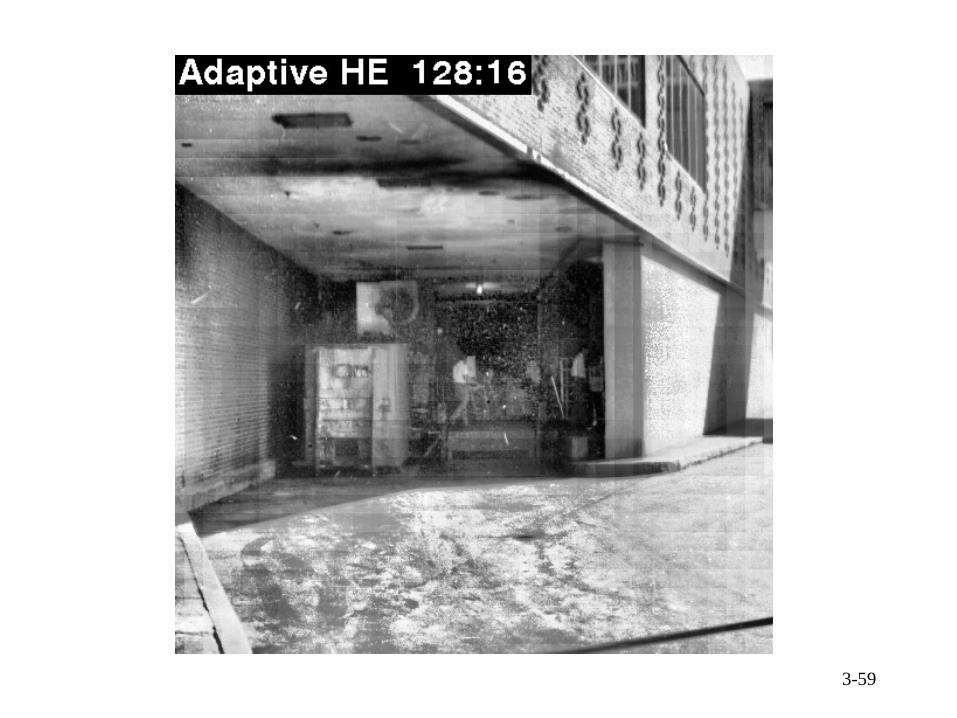
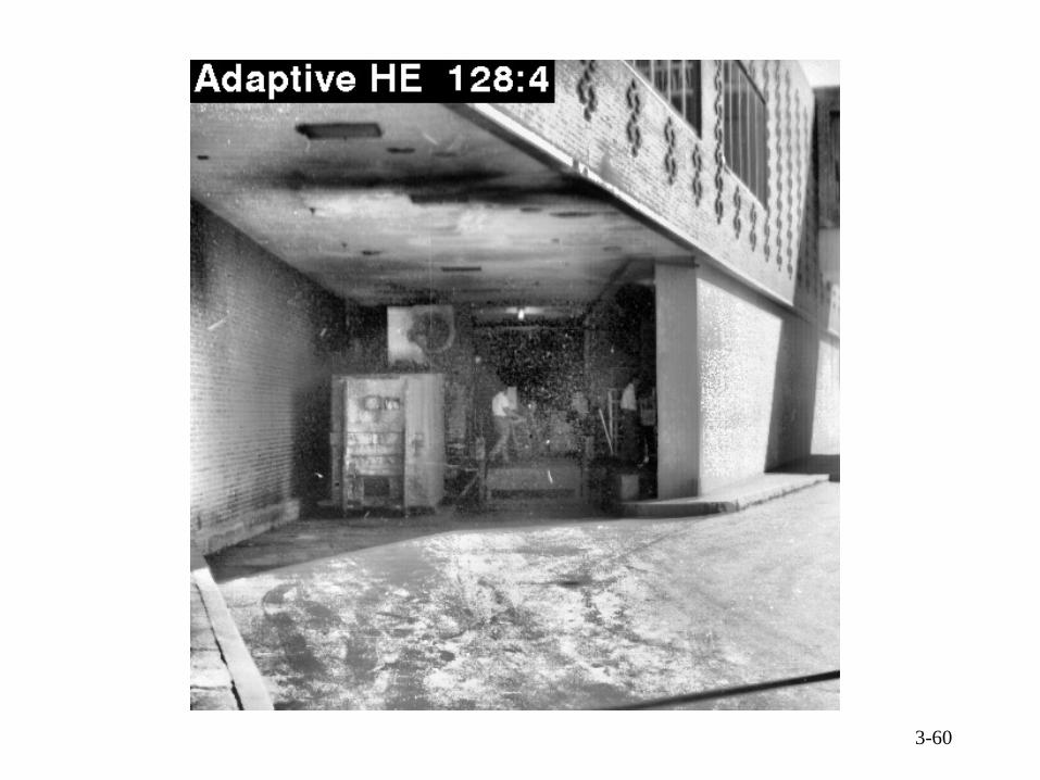
Moving Window AHE

The HE LUT for large outer window (e.g., 128 × 128) is computed, but applied only to the small inner window (e.g., 16 × 16). The inner window is then shifted and the process is repeated.

Outer windowInner window

3-58

3-59

3-60

3-61

3-62

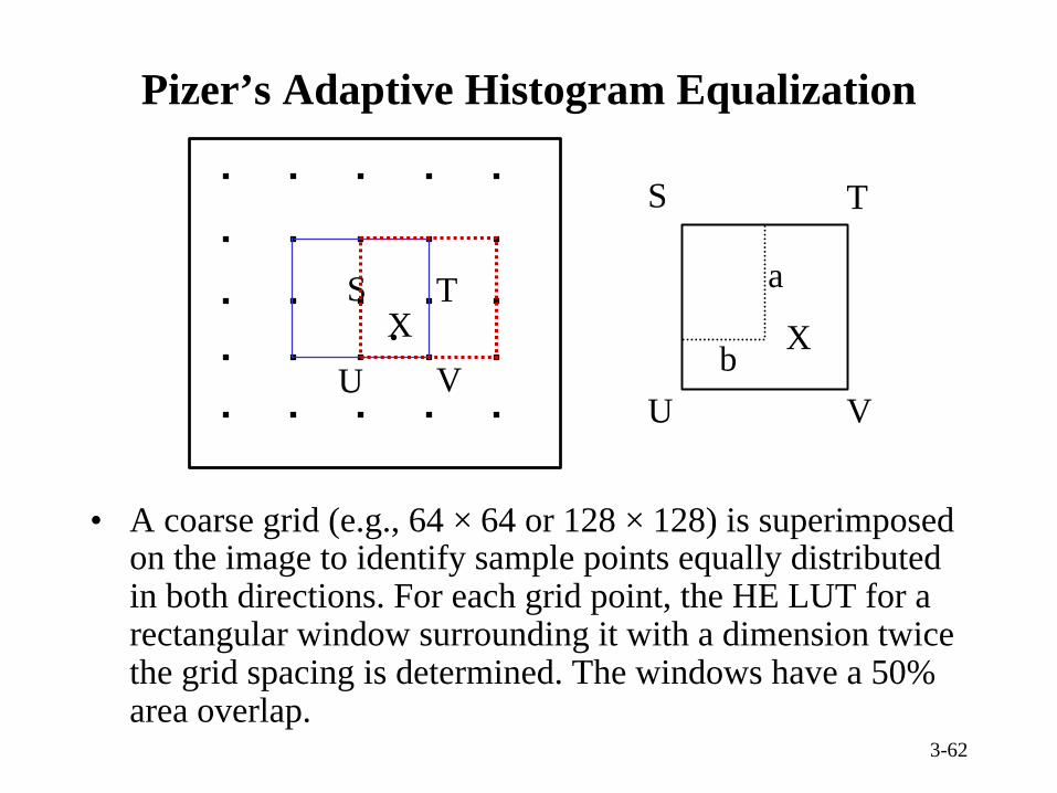
S T

U V

Xb

a S

U V

TX

Pizer’s Adaptive Histogram Equalization

• A coarse grid (e.g., 64 × 64 or 128 × 128) is superimposed on the image to identify sample points equally distributed in both directions. For each grid point, the HE LUT for a rectangular window surrounding it with a dimension twice the grid spacing is determined. The windows have a 50% area overlap.

3-63

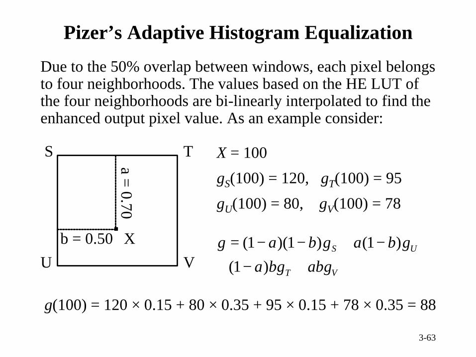
Pizer’s Adaptive Histogram Equalization

Due to the 50% overlap between windows, each pixel belongs to four neighborhoods. The values based on the HE LUT of the four neighborhoods are bi-linearly interpolated to find the enhanced output pixel value. As an example consider:

X = 100

gS(100) = 120, gT(100) = 95

gU(100) = 80, gV(100) = 78

VU

S T

a = 0.70

b = 0.50 X

g(100) = 120 × 0.15 + 80 × 0.35 + 95 × 0.15 + 78 × 0.35 = 88

VT

US

gabgbagbagbag

+−++−+−−=

)1()1( )1)(1(

3-64

3-65

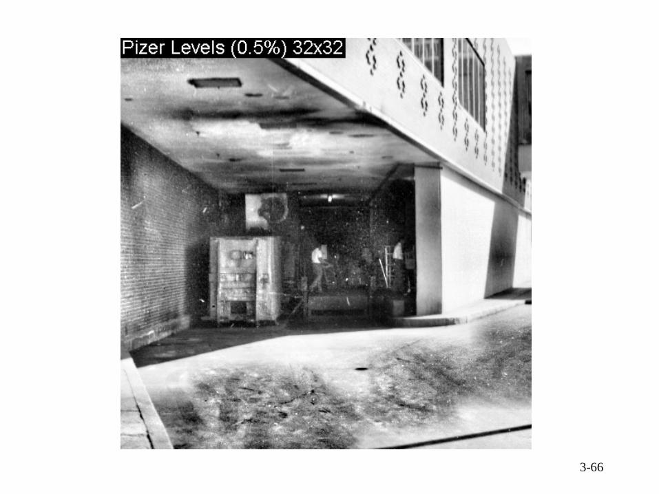
3-66

3-67

3-68

3-69

3-70

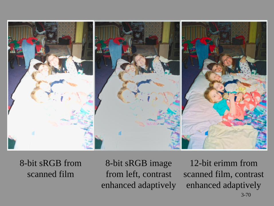
8-bit sRGB from scanned film

8-bit sRGB image from left, contrast

enhanced adaptively

12-bit erimm from scanned film, contrast enhanced adaptively

3-71

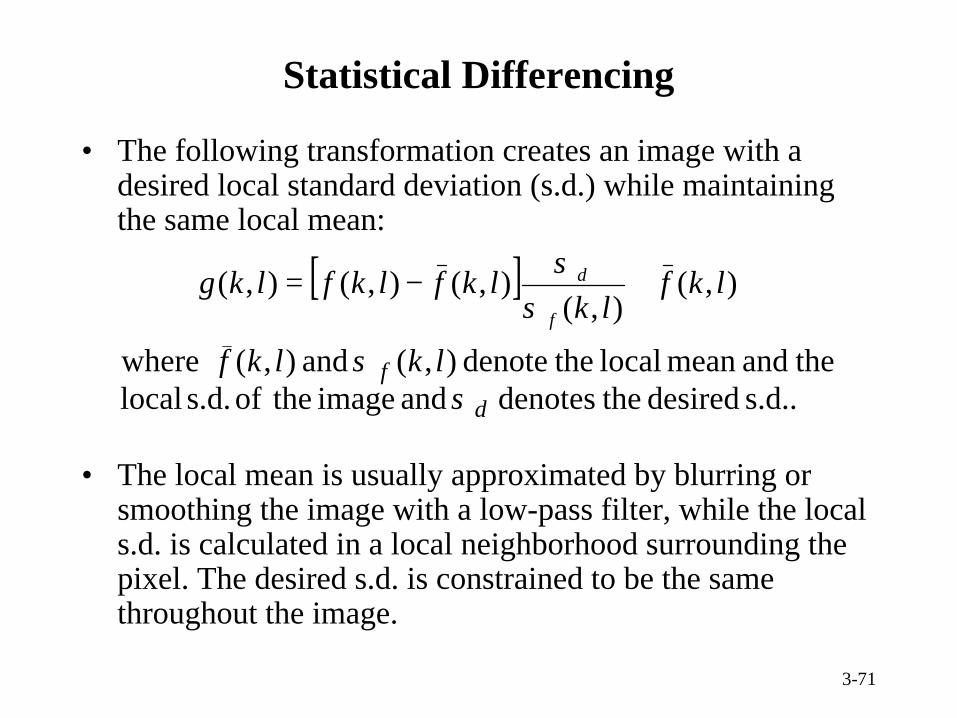
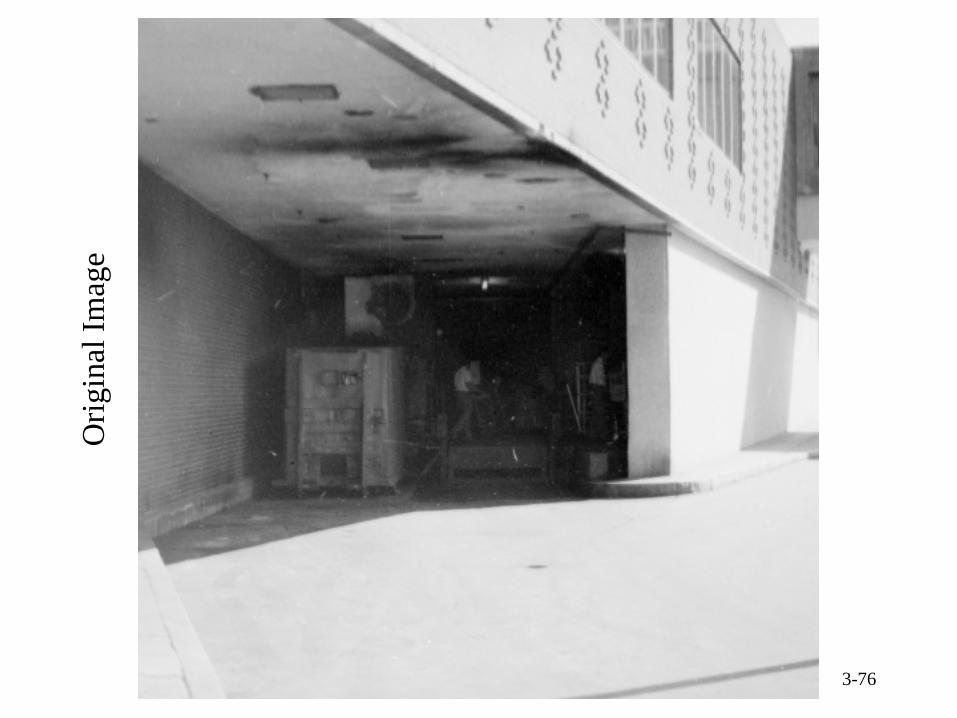
Statistical Differencing

• The following transformation creates an image with a desired local standard deviation (s.d.) while maintaining the same local mean:

• The local mean is usually approximated by blurring or smoothing the image with a low-pass filter, while the local s.d. is calculated in a local neighborhood surrounding the pixel. The desired s.d. is constrained to be the same throughout the image.

s.d.. desired thedenotes and image theof s.d. local theandmean local thedenote ),( and ),( where

d

f lklkfσ

σ

[ ] ),(),(

),(),(),( lkflk

lkflkflkgf

d +−=σ

σ

3-72

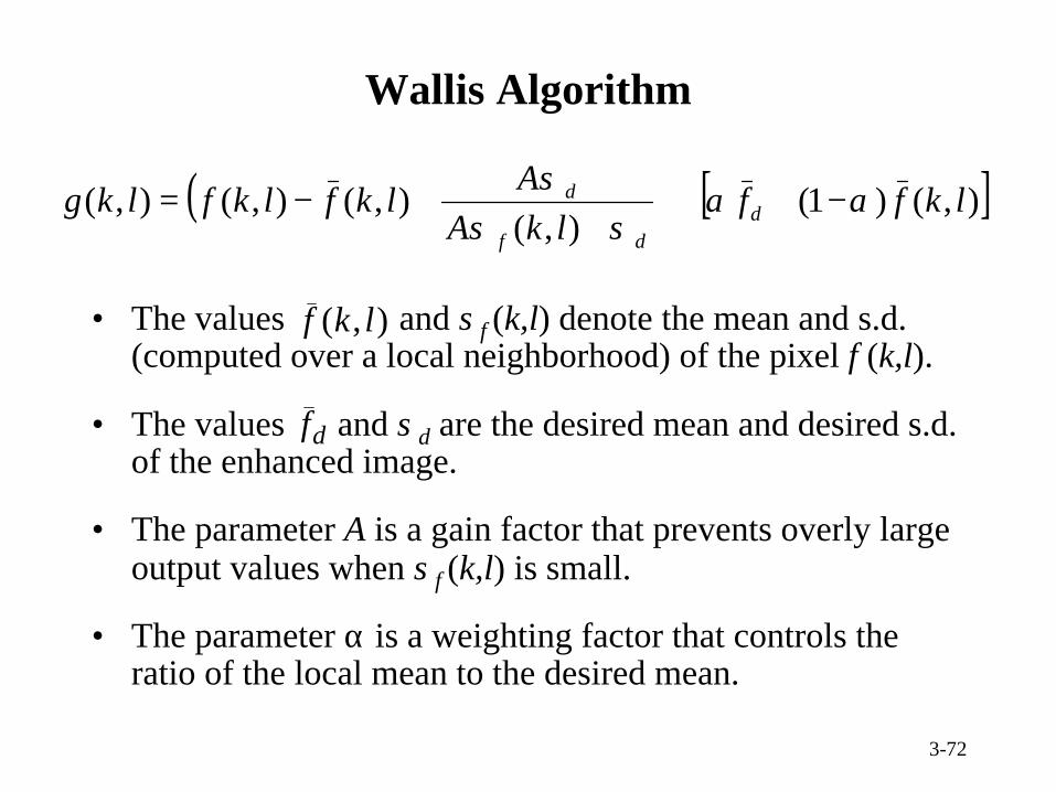
Wallis Algorithm

• The values and σf (k,l) denote the mean and s.d. (computed over a local neighborhood) of the pixel f (k,l).

• The values and σd are the desired mean and desired s.d. of the enhanced image.

• The parameter A is a gain factor that prevents overly large output values when σf (k,l) is small.

• The parameter α is a weighting factor that controls the ratio of the local mean to the desired mean.

( ) [ ]),()1(),(

),(),(),( lkfflkA

Alkflkflkg d

df

d αασσ

σ−++

+−=

),( lkf

df

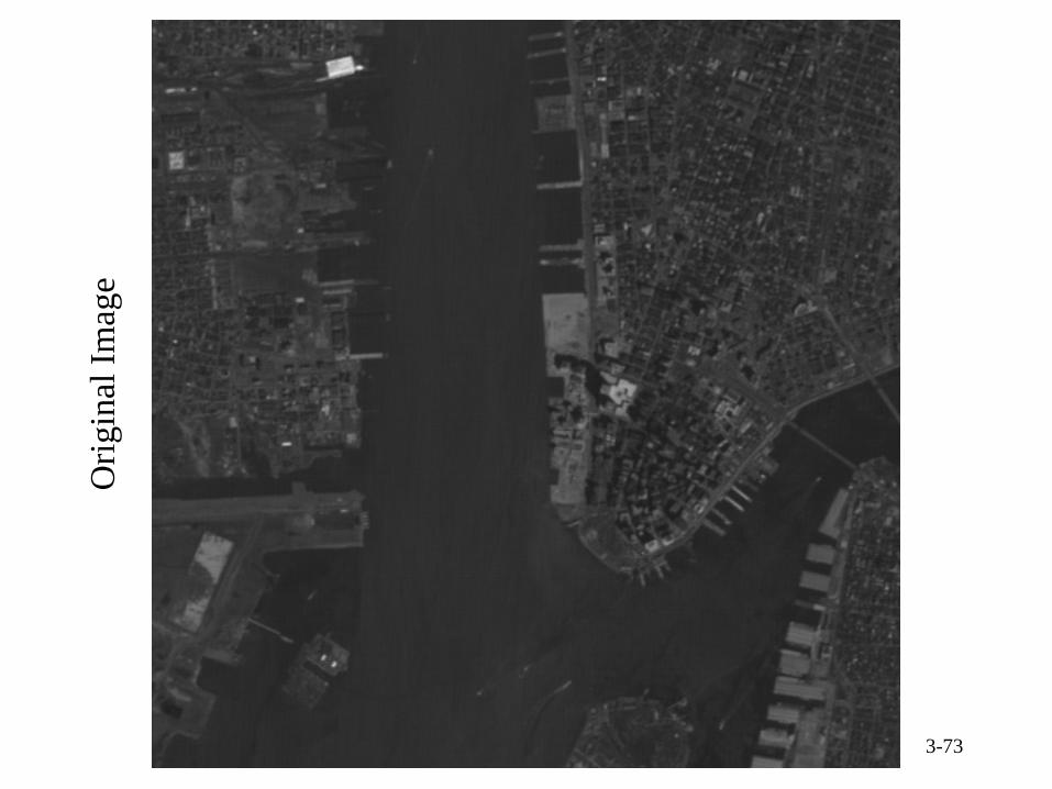
3-73

Ori

gina

l Im

age

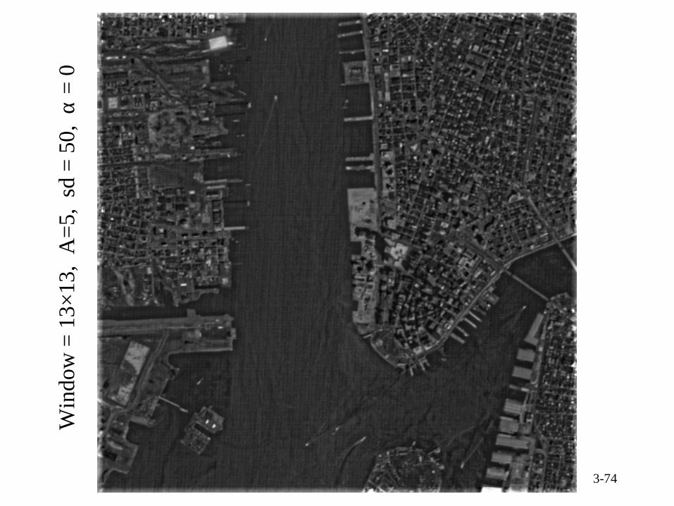
3-74

Win

dow

= 1

3×13

, A

=5,

sd=

50,

α=

0

3-75

Win

dow

= 1

3×13

, A

=5,

sd=

80,

α=

0

3-76

Ori

gina

l Im

age

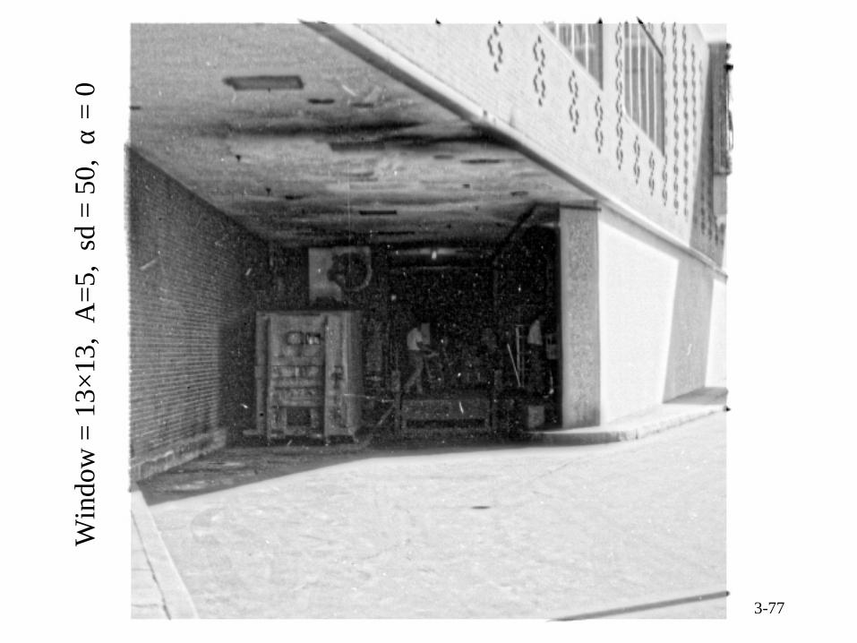
3-77

Win

dow

= 1

3×13

, A

=5,

sd=

50,

α=

0

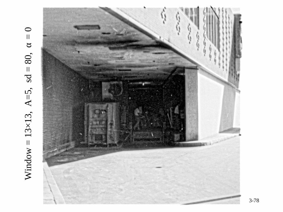
3-78

Win

dow

= 1

3×13

, A

=5,

sd=

80,

α=

0

3-79

Win

dow

= 1

3×13

, A

=10,

sd

= 50

, α

= 0

3-80

Adaptive Dynamic Range Compression (DRC)

+( )ff −

f ff

+-

• Contrast enhancement can be done by breaking up the image into a low-frequency (pedestal) and high-frequency (detail) component and applying a LUT to pedestal image.

Low-PassFilter

+

DR-reducedpedestal image

LUT