3 development of a multi-modal aimsun model for...

A Mesoscopic DTA Multi Modal Aimsun Model for the GTA

Islam Taha, PhD CandidateBaher Abdulhai, PhDAmer Shalaby, PhD

Outline

The case for Dynamic

Traffic Assignment

The UofT Aimsun GTA

DTA model

Why do we need dynamic system representation and modelling? We need accurate representation of cost of travel:

in transportation planning in traffic engineering /operations

Static Network Analysis and Models: variables of interest that are time-invariant the concept of user equilibrium traffic assignment may or may not directly correlate with physical measures describing congestion (e.g. flow

density ..)

Dynamic Network Analysis and Models: more detailed representation of the interaction between travel choices, traffic flows, and

time and cost measures in not only spatially but also temporally coherent manner. Dynamic Traffic Assignment combines time-dependent route choice (assignment) concepts

and traffic flow theory

3

Typical VDF (BRP) Simple Traffic Model 4

Modelling Congestion: Static vs. Dynamic Models

Drawbacks and Limitations of Static Models

Conceptual Drawbacks Allow V/C >1, has no intuitive meaning, does not correspond to reality

or real measurements Restricted to FIFO Cannot model traffic moving in different lanes Inflow = Outflow, i.e.

Single value of link flow Steady state representation only Cannot capture temporal congestion spread and spill-back

Application Limitations: cannot do Signal synchronization HOV and HOT Lanes Evacuation, congestion pricing optimization ITS applications, ATMS, ATIS, RM, Adaptive Control

5

Now: What is Dynamic Traffic Assignment (DTA)?

In a network with many OD zones and a time period of interest, for each OD pair and departure time, all used routes have equal and lowest experienced travel time (generalized cost).

Compared with Static Traffic Assignment below:

In a network with many OD zones, for each OD pair, all used routes have equal and lowest travel time (generalized cost).

6

Experienced vs Instantaneous Travel Time

3

2

2

1

1

4

3

3

2

1

4

6

5

3

1

Link travel timewhen entering thelink at each minute

Travel time for departing at min 1 = 3 min


4

(a) Instantaneous travel time calculation

3

2

2

1

1

4

3

3

2

1

4

6

5

3

1

Link travel timewhen entering thelink at each minute



4

(b) Experienced travel time calculation

• Note how the modelling period is sliced into assignment intervals• Experienced travel time is much different from instantaneous

and can only be realized after the fact of going through the trip

7

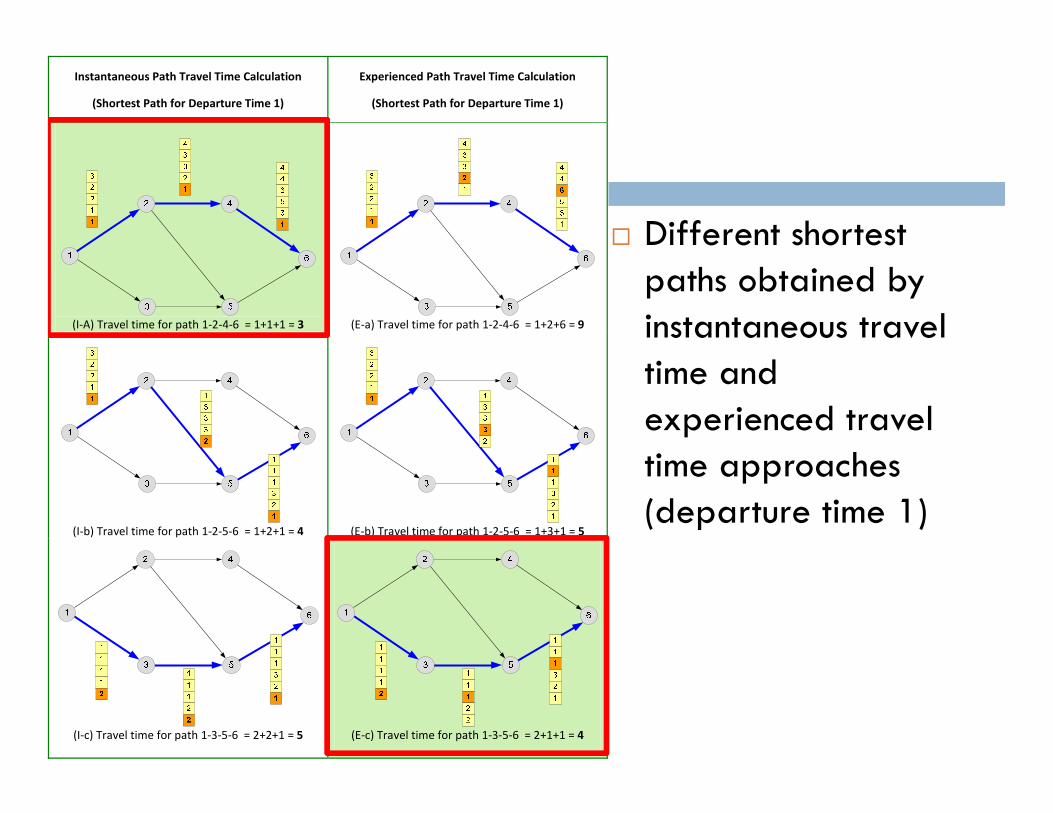
Different shortest paths obtained by instantaneous travel time and experienced travel time approaches (departure time 1)

Instantaneous Path Travel Time Calculation

(Shortest Path for Departure Time 1)

Experienced Path Travel Time Calculation

(Shortest Path for Departure Time 1)

(I‐A) Travel time for path 1‐2‐4‐6 = 1+1+1 = 3

(E‐a) Travel time for path 1‐2‐4‐6 = 1+2+6 = 9

(I‐b) Travel time for path 1‐2‐5‐6 = 1+2+1 = 4

(E‐b) Travel time for path 1‐2‐5‐6 = 1+3+1 = 5

(I‐c) Travel time for path 1‐3‐5‐6 = 2+2+1 = 5

(E‐c) Travel time for path 1‐3‐5‐6 = 2+1+1 = 4

Simulation DUE/DTA Algorithmic Structure

9

What to use iterative DTA for:10

Operational planning (or planning for operations) aimed at making planning decisions that are likely to induce a spatio-temporal (temporal, spatial or both) pattern shift of traffic among different roadway facilities at a corridor or network wide level.

Illustration: Static vs. Dynamic Modelling

Illustrative Example: consider 2 identical O-D pairs with 4000 vph demand 4 identical routes, each with capacity of 2000 vph Routes b and c pass through a bridge with capacity of

4000 vph

11

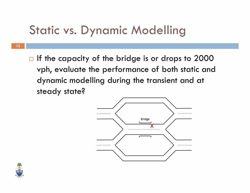
Static vs. Dynamic Modelling

If the capacity of the bridge is or drops to 2000 vph, evaluate the performance of both static and dynamic modelling during the transient and at steady state?

x

12


At steady state Static Dynamic

Before capacity drop

All routes carry 2000 vph All routes carry 2000

After capacity drop • Some traffic shifts to outer routes

• On the bridge flows are greater than capacity

• Just before the bridge, flows are less than capacity which implies abnormally high speeds

• Precise amount of traffic shifts to outer routes

• On bridge, flows cannot exceed capacity

• Congestion spills back to the origins affecting all upstream links

13


Static Dynamic

Steady state traffic flows at the bridge

Flows greater than capacity on all routes (v/c >1)

Flows limited to the capacity

Steady state traffic flows upstream of bridge

Flows less than capacity and high speeds

Congestion spills back upstream from the bridge

Transient state Cannot be modelled Properly captures gradual congestion spreading on inner routes (time variant travel costs)

Can be modelled in both one-shot and iterative

14

Static vs. Dynamic Modelling • Transient state after capacity drop: Congestion

Static:

Dynamic:

15

Static vs. Dynamic Modelling • Steady state after capacity drop: Congestion

Static:

Dynamic:

16

Policy implications

If the purpose of the analysis is to identify the bridge for expansion (typical planning), both approaches would somewhat do, despite the misrepresentation of static.

If the purpose of the analysis is to adjust the spatio temporalpatterns of traffic (changes in departure time, route choice etc.), which is typical in over congested networks, only dynamic models should be used, static cannot do and can be misleading or even wrong (tolling the outer routes for instance).

17

Mesoscopic DTA Multi-modal Model for the GTA

Mesoscopic model covers most of the GTA, focusing on freeways,

major arterials, and arterials carrying TTC vehicles

Dynamic traffic assignment captures how congestion evolves over

time

Multi-modal model includes driving, transit (GO, TTC, parts of

MiWay), and park-and-ride

The model simulates AM peak trips

18

Model Development

12,986 Nodes29,422 Links26,769 Km

HOV Tolled Freeway

Ramp Arterial

Metering

Signalized

Non-signalized

19

Model Development

Destination Zones

1 2 ⋯ 1497

Orig

in Zon

es 1 0 2300 ⋯ 9847

2 9984 2208 ⋯ 0

⋮ ⋮ ⋮ ⋱ ⋮

1497 6788 9188 ⋯ 398

Destination Zones

1 2 ⋯ 1497

Orig

in Zon

es 1 0 2300 ⋯ 9847

2 9984 2208 ⋯ 0

⋮ ⋮ ⋮ ⋱ ⋮

1497 6788 9188 ⋯ 398

Destination Zones

1 2 ⋯ 1497

Orig

in Zon

es 1 0 2300 ⋯ 9847

2 9984 2208 ⋯ 0

⋮ ⋮ ⋮ ⋱ ⋮

1497 6788 9188 ⋯ 398

Destination Zones

1 2 ⋯ 1497

Orig

in Zon

es 1 0 2300 ⋯ 9847

2 9984 2208 ⋯ 0

⋮ ⋮ ⋮ ⋱ ⋮

1497 6788 9188 ⋯ 398

1497 Traffic ZonesTravel Demand

36 Million records

During AM Peak436,000 Hourly Trips

20

Model Development

Land Information Ontario (LIO)

GIS database (links, nodes, signals, etc.)

Transportation Tomorrow Survey (TTS)

Travel demand and traffic zones

21

Model Development

The GIS model

Auxiliary lanes Speed limits Traffic signals

Travel demand data

Flip-flopping data trend

Background demand

Intra-zonal demand

22

Model Development: Travel Demand

0

50000

100000

150000

200000

250000

300000

6:00

6:15

6:30

6:45

7:00

7:15

7:30

7:45

8:00

8:15

8:30

8:45

9:00

9:15

9:30

9:45

Tota

l num

ber

of tr

ips

Time interval

Original Demand Filtered GTA Demand

0

50000

100000

150000

200000

250000

300000

6:00

6:15

6:30

6:45

7:00

7:15

7:30

7:45

8:00

8:15

8:30

8:45

9:00

9:15

9:30

9:45

Tota

l num

ber

of tr

ips

Time interval

Original Demand Filtered GTA Demand

The GIS model


Travel demand data

Flip-flopping behavior

Background demand

Intra-zonal demand

23


The GIS model


Travel demand data


Background demand

Intra-zonal demand

05000

1000015000200002500030000

6:00

6:15

6:30

6:45

7:00

7:15

7:30

7:45

8:00

8:15

8:30

8:45

9:00

9:15

9:30

9:45To

tal n

umbe

r of

trip

sTime interval

Incoming Traffic Outgoing TrafficThrough Traffic

24


The GIS model


Travel demand data


Background demand

Intra-zonal demand

0

50000

100000

150000

200000

250000

6:00

6:15

6:30

6:45

7:00

7:15

7:30

7:45

8:00

8:15

8:30

8:45

9:00

9:15

9:30

9:45

Tota

l num

ber

of tr

ips

Time interval

Total GTA and Background Demand

25

DTA Setup

• Mesoscopic DUE

• Iterative (30 iterations)

• Experienced travel times

• Road attractiveness:

• Jam density:

• Fixed reaction time:

26

DTA Outputs

• Flow, speed, density, queue length, travel time, …

• Network-wide statistics

• Sections, nodes, traffic signals, turns, …

• Vehicle trajectories

27

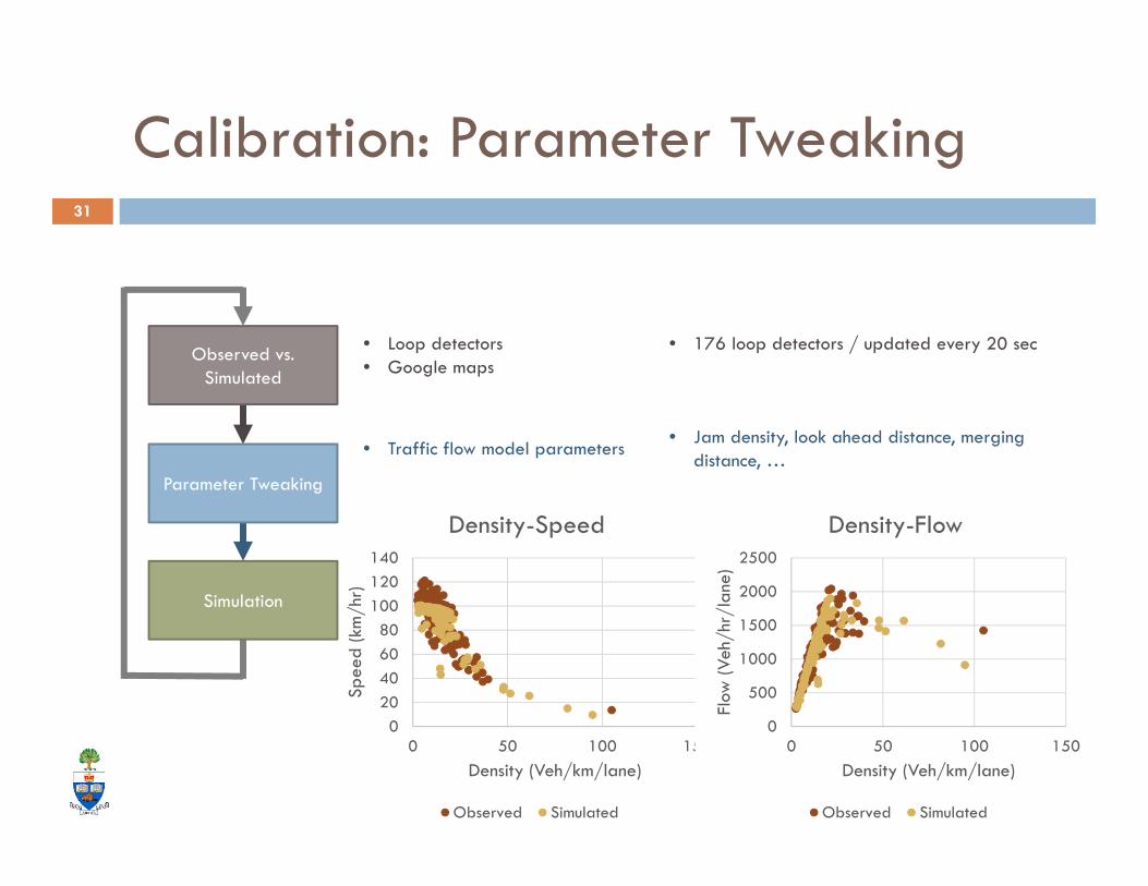
Model Calibration

Observed vs. Simulated

Parameter Tweaking

Simulation

28

Calibration: Observed vs Simulated


Parameter Tweaking

Simulation

• Loop detectors• Google maps

• 176 loop detectors / updated every 20 sec

0

2000

4000

6000

8000

10000

0 5000 10000

Sim

ulat

ed F

low

s

Observed Flows

29

Calibration: Observed vs Simulated


Parameter Tweaking

Simulation



01000200030004000500060007000

401-

EC -

E O

F KI

PLIN

G40

1-EC

- W

OF…

401-

EC -

E O

F…40

1-EC

- W

OF…

401-

EC -

W O

F…40

1-EC

- E

OF…

401-

EC -

W O

F 40

040

1-EC

- E

OF

400

401-

EC -

E O

F JA

NE

401-

ET -

E O

F JA

NE

401-

EC -

W O

F KE

ELE

401-

EC -

AT

KEEL

E40

1-EC

- E

OF

KEEL

E40

1-EC

- E

OF

KEEL

E40

1-EC

- W

OF…

401-

EC -

E O

F…40

1-EC

- W

OF…

401-

EC -

W O

F…40

1-EC

- W

OF…

401-

EC -

AT

YON

GE

401-

EC -

E o

f Yo

nge

401-

EC -

W o

f…40

1-EC

- E

of

Bayv

iew

401-

EC -

E o

f Le

slie

401-

ET -

E o

f Le

slie

401-

EC -

E o

f D

on M

ills

401-

EC -

AT…

401-

EC -

AT

NEI

LSO

N40

1-EC

- E

. OF…

401-

EC -

E. O

F…40

1-EC

- A

T…

Flow

(V

eh/h

r)

Driving Directions

HWY401 Collector EB

Observed

Simulated

30

Calibration: Parameter Tweaking


• Traffic flow model parameters• Demand tables• Network geometry-related

parameters


• Jam density, look ahead distance, merging distance, …

• OD pairs travelling over specific corridors• Speed limits, signal timing, number of lanes,

…

020406080

100120140

0 50 100 150

Spee

d (k

m/h

r)

Density (Veh/km/lane)

Density-Speed

Observed Simulated

0

500

1000

1500

2000

2500

0 50 100 150Fl

ow (V

eh/h

r/la

ne)

Density (Veh/km/lane)

Density-Flow

Observed Simulated

Simulation

Parameter Tweaking


31

Calibration : Demand Tweaking


Parameter Tweaking

Simulation



parameters



• OD pairs travelling over specific corridors• Speed limits, signal timing, number of lanes,

…

0

50

100

York St SpadinaAve

BathurstSt

JamesonAve

DowlingAve

Ellis Ave

Speed (kph

)

Travel Direction

Before

Observed Simulated

0

50

100

York St SpadinaAve

BathurstSt

JamesonAve

DowlingAve

Ellis Ave

Spee

d (k

ph)

Travel direction

After

Observed Simulated

32

Calibration: Miscellaneous


Parameter Tweaking

Simulation

• Loop detectors• Camera feeds• Google maps


parameters

• 35 million daily readings / updated every 20 sec


• OD pairs travelling over specific corridors• Signal timing, number of lanes, …

33

Calibration: GEH34

Ongoing Work

Transit layers

Joint departure time and mode choice model

Concurrent optimization of dynamic congestion

pricing and variable transit fares

35

Demo36

Thank You!

3 development of a multi-modal aimsun model for...

Documents